Calabi–Yau structures on Rabinowitz Fukaya categories

Abstract.

In this paper, we prove that the derived Rabinowitz Fukaya category of a Liouville domain $M$ of dimension $2n$ is $(n-1)$-Calabi–Yau assuming the wrapped Fukaya category of $M$ admits an at most countable set of Lagrangians that generate it and satisfy some finiteness condition on morphism spaces between them.

1. Introduction

Rabinowitz Floer homology is a Floer homology associated to a contact hypersurface of a symplectic manifold, which was first introduced by Cieliebak and Frauenfelder [CF09]. In particular, in [CFO10], Cieliebak, Oancea and Frauenfelder proved that the Rabinowitz Floer homology $RFH_{*}(M)$ of a Liouville domain $M$ of dimension $2n$ fits into a long exact sequence

$$\dots\to SH^{-*}(M)\to SH_{*}(M)\to RFH_{*}(M)\to SH^{-*+1}(M)\to\cdots.$$ (1.1)

Here, the map $SH^{-*}(M)\to SH_{*}(M)$ factors through

where the vertical arrows $c^{*}:SH^{-*}(M)\to H_{*+n}(M)$ and $c_{*}:H_{*+n}(M,\partial M)\to SH_{*}(M)$ are induced by quotient maps and inclusion maps between Floer complexes in certain action windows.

In [Ven18, CO20], this map was understood as a continuation map. Indeed, they consider Floer homologies for Hamiltonians that are linear with negative slopes and positive slopes at infinity and then consider the continuation map from the former one to the latter one. This leads to a new approach to defining Rabinowitz Floer complex as a mapping cone of a continuation map between two Floer complexes.

Adapting this idea to an open string analogue of Rabinowitz Floer homology, Ganatra, Gao and Venkatesh [GGV22] recently introduced Rabinowitz wrapped Fukaya category of a Liouville domain. For a Liouville domain $M$, objects of the Rabinowitz wrapped Fukaya category $\mathcal{RW}(M)$ are certain Lagrangian submanifolds of $M$ and the morphism space between two Lagrangian submanifolds $L_{0}$ and $L_{1}$ of $M$ is given by the mapping cone of the continuation map from the Floer complex $CW_{*}(L_{0},L_{1})$ for wrapped Floer homology to that $CW^{*}(L_{0},L_{1})$ for wrapped Floer cohomology. Namely, the Rabinowitz Floer complex between $L_{0}$ and $L_{1}$ is given by

$$RFC^{*}(L_{0},L_{1})=\mathrm{Cone}(c:CW_{n-*}(L_{0},L_{1})\to CW^{*}(L_{0},L_{1}))$$

for the continuation map $c$. Furthermore, if $M$ is Weinstein, they showed that its Rabinowitz wrapped Fukaya category $\mathcal{RW}(M)$ is quasi-equivalent to the formal punctured neighborhood of infinity $\widehat{\mathcal{W}}_{\infty}(M)$ of the wrapped Fukaya category $\mathcal{W}(M)$. In particular, the latter one $\widehat{\mathcal{W}}_{\infty}(M)$ is further shown to be quasi-equivalent to the quotient $\mathcal{W}(M)/\mathcal{F}(M)$ for the compact Fukaya category $\mathcal{F}(M)$ when it is a Koszul dualizing subcategory of $\mathcal{W}(M)$.

Meanwhile, in our previous work [BJK22], we consider plumbings of $T^{*}S^{n}$ along a tree for $n\geq 3$. The main result is that, for such a Weinstein manifold, the derived wrapped Fukaya category, the derived compact Fukaya category, and the collection of cocore disks $(D^{\pi}\mathcal{W},D^{\pi}\mathcal{F},L)$ form a Calabi–Yau triple. As a consequence, the quotient category $D^{\pi}\mathcal{W}/D^{\pi}\mathcal{F}$ becomes an $(n-1)$-Calabi–Yau (generalized) cluster category.

Here, Calabi–Yau property is defined as follows.

Definition 1.1.

A triangulated category $\mathcal{C}$ over a field $\mathbb{K}$ is said to be $n$-Calabi–Yau for some $n\in\mathbb{Z}$ if, for all objects $X$ and $Y$ of $\mathcal{C}$,

• $\dim\mathrm{Hom}_{\mathcal{C}}(X,Y)<\infty$ and

• there exists a non-degenerate pairing

  $$\beta_{X,Y}:\mathrm{Hom}_{\mathcal{C}}(Y,X[n])\times\mathrm{Hom}_{\mathcal{C}}(X,Y)\to\mathbb{K},$$

  which is bifunctorial.

The bifunctoriality means that $\beta_{X,Y}$ defines a natural transformation between two functors from $\mathcal{C}^{op}\times\mathcal{C}$ to $\mathbb{K}$ given by

$$(X,Y)\mapsto\mathrm{Hom}_{\mathcal{C}}(X,Y)$$

and

$$(X,Y)\mapsto\mathrm{Hom}_{\mathcal{C}}(Y,X[n])^{\vee}.$$

Since the compact Fukaya category is known to be Koszul dual to the wrapped Fukaya category in this case [EL17b, EL17a], this means that the derived Rabinowitz wrapped Fukaya category of the plumbings carry an $(n-1)$-Calabi–Yau cluster structure.

At this point, the following question arises naturally:

When does the derived Rabinowitz wrapped Fukaya category admit a Calabi–Yau structure?

In this paper, we give a partial answer to this question. Indeed, under the assumption that the wrapped Fukaya category of a Liouville domain $M$ with $2c_{1}(M)=0$ is generated by an at most countable family of Lagrangians of $M$, we provide equivalent conditions for its derived Rabinowitz wrapped Fukaya category being Calabi–Yau. It can be stated as follows.

Theorem 1.2 (Theorem 3.6).

Let $M$ be a Liouville domain of dimension $2n$ with $2c_{1}(M)=0$ and let $b\in H^{2}(M,\mathbb{Z}/2)$ be a background class. Assume that $M$ admits a set of admissible Lagrangians $\{L_{i}\}_{i\in I}$ for some at most countable set $I$ generating $\mathcal{W}_{b}(M)$. Then the following are equivalent.

1. The derived Rabinowitz wrapped Fukaya category $D^{\pi}\mathcal{RW}(M)$ is $(n-1)$-Calabi–Yau.

2. For all $i,j\in I$ and $k\in\mathbb{Z}$, $\dim RFH^{k}(L_{i},L_{j})<\infty$.

3. For all $i,j\in I$ and $k\in\mathbb{Z}$, $\dim HW^{k}(L_{i},L_{j})<\infty$.

Here, $RFH^{*}(L_{i},L_{j})$ denotes the homology of the Rabinowitz Floer complex $RFC^{*}(L_{i},L_{j})$.

We remark that, it was proved in [CHO20, Theorem 1.3] that, under certain topological assumptions, there is a graded open-closed TQFT structure on the pair of a (degree shifted) Rabinowitz Floer homology $RF\mathbb{H}_{*}(\partial M)$ of a Liouville domain $M$ and a (degree shifted) Rabinowitz Floer homology ${RF}\mathbb{H}_{*}(\partial L)$ of a Lagrangian submanifold $L$ of $M$ having a cylindrical Legendrian end. Furthermore, it was explained that this result holds either both ${RF}\mathbb{H}_{*}(\partial M)$ and $RF\mathbb{H}_{*}(\partial L)$ are of finite type, meaning that they are finite dimensional in each degree, or they are endowed with additional filtrations defined using actions. In terms of our cohomological convention, this implies the existence of a nondegenerate pairing between $RFH^{*}(L,L)$ and $RFH^{n-1-*}(L,L)$.

Theorem 1.2 can be viewed as a partial extension of the result of [CHO20] to a categorical level under the finite type assumption in the sense that we prove that the duality pairing extends to any pair of objects of derived Rabinowitz wrapped Fukaya category. This extension was available since we worked with $A_{\infty}$-category and operators on chain level. We guess that many experts would have already expected Theorem 1.2 to be true.

Let us now return to how to prove Theorem 1.2. We prove it by showing (1) $\Rightarrow$ (2) $\Rightarrow$ (3) $\Rightarrow$ (1). Here, we provide the proofs of the implications (1) $\Rightarrow$ (2) and (2) $\Rightarrow$ (3) and briefly explain the strategy for the proof of the implication (3) $\Rightarrow$ (1), which will be proved in Section 3.

The first implication (1) $\Rightarrow$ (2) follows from the definition of Calabi–Yau property and the fact that $\mathrm{Hom}_{D^{\pi}\mathcal{RW}(M)}(L_{i},L_{j}[k])\cong RFH^{k}(L_{i},L_{j})$ by definition of the derived Rabinowitz wrapped Fukaya category $D^{\pi}\mathcal{RW}(M)$.

For the second implication (2) $\Rightarrow$ (3), consider the long exact sequence:

$$\dots\to HW_{n-*}(L_{i},L_{j})\xrightarrow{c_{*}}HW^{*}(L_{i},L_{j})\to RFH^{*}(L_{i},L_{j})\to HW_{n-*-1}(L_{i},L_{j})\xrightarrow{c_{*}}\cdots,$$ (1.2)

which is a consequence of the definition of the Rabinowitz Floer complex $RFC^{*}(L_{i},L_{j})$. In Section 2, we will see that the continuation map $c:CW_{n-*}(L_{i},L_{j})\to CW^{*}(L_{i},L_{j})$ factors through

where $c_{-\epsilon,\epsilon}:CF^{*}(L_{i},L_{j};H_{-\epsilon})\to CF^{*}(L_{i},L_{j};H_{\epsilon})$ is a continuation map between Floer complexes of $L_{i}$ and $L_{j}$ for Hamiltonians $H_{\pm\epsilon}$ linear at infinity with slope $\pm\epsilon$ for a sufficiently small $\epsilon>0$. This means that the image of the continuation $c_{*}:HW_{n-*}(L_{i},L_{j})\to HW^{*}(L_{i},L_{j})$ is finite-dimensional since $\dim HF^{*}(L_{i},L_{j};H_{\pm\epsilon})$ is finite. Therefore, if $HW^{k}(L_{i},L_{j})$ is infinite-dimensional, then $RFH^{k}(L_{i},L_{j})$ is infinite-dimensional as well.

Finally, the proof of the last implication (3) $\Rightarrow$ (1) relies on the duality between the wrapped Floer cohomology $HW^{*}(L_{0},L_{1})$ and the wrapped Floer homology $HW_{*}(L_{1},L_{0})$ for Lagrangians $L_{0}$ and $L_{1}$, which comes from the natural duality between $CF^{*}(L_{0},L_{1};H_{a})$ and $CF^{n-*}(L_{1},L_{0};-H_{a})$ for a Hamiltonian $H_{a}$ linear at infinity with slope $a\in\mathbb{R}$.

The duality between $HF^{*}(L_{0},L_{1};H_{a})$ and $HF^{n-*}(L_{1},L_{0};H_{-a})$ can be obtained as the composition of the pair-of-pants product

$$HF^{n-*}(L_{1},L_{0};H_{-a-\epsilon})\otimes HF^{*}(L_{0},L_{1};H_{a})\to HF^{n}(L_{0},L_{0};H_{-\epsilon})$$

and the integration

$$HF^{n}(L_{0},L_{0};H_{-\epsilon})\cong H^{n}(L_{0},\partial L_{0};\mathbb{K})\to\mathbb{K}$$

for $\epsilon>0$ sufficiently small so that the following are isomorphic:

$$HF^{n-*}(L_{1},L_{0};H_{-a})\cong HF^{n-*}(L_{1},L_{0};H_{-a-\epsilon}).$$

Since both of these operators originate from operators on chain complex level, we construct chain maps

$$\overline{\alpha} :CW^{*}(L_{0},L_{1})\to CW_{*}(L_{1},L_{0})^{\vee},$$

$$\overline{\gamma} :CW_{*}(L_{0},L_{1})\to CW^{*}(L_{1},L_{0})^{\vee},$$

which give the duality explained above. Then we construct a chain map

$$\overline{\beta}:RFC^{*}(L_{0},L_{1})\to RFC^{n-1-*}(L_{1},L_{0})^{\vee}$$

so that the following diagram commutes:

We found it easier to use linear Hamiltonians to construct such chain maps, rather than quadratic Hamiltonians as in [GGV22].

Although the chain map $\overline{\gamma}$ is always a quasi-isomorphism, the same cannot be said for $\overline{\alpha}$ due to the same reason as in [CO18, Section 3.3]. However, the condition that $HW^{k}(L_{0},L_{1})$ is finite-dimensional for each degree $k\in\mathbb{Z}$ ensures that $\overline{\alpha}$ is a quasi-isomorphism as well. As a result, the chain map $\overline{\beta}$ becomes a quasi-isomorphism under the assumption. Finally, we observe that the chain map $\overline{\beta}$ naturally extends to the triangulated envelope and gives a Calabi–Yau paring on the derived Rabinowitz wrapped Fukaya category.

Let us now give a brief overview of this paper. In Section 2, we construct Rabinowitz Fukaya category using linear Hamiltonians as mentioned above. In Section 3, we construct the chain maps $\overline{\alpha}$, $\overline{\beta}$ and $\overline{\gamma}$ that fit into the above commutative diagram and show that these are quasi-isomorphisms under the assumption that the condition (3) of Theorem 1.2 is satisfied. Then we show that it extends to the triangulated envelope. Finally, in Section 4, we provide three examples of Liouville domains for which the condition (3) of Theorem 1.2 is satisfied. This includes cotangent bundles of simply-connected closed manifolds, plumbings of $T^{*}S^{n}$ along a tree and Weinstein domains with a periodic Reeb flow on the boundary.

Acknowledgements.

We thank Cheol-Hyun Cho, Jungsoo Kang, Yeongrak Kim, Yoosik Kim and Yong-Geun Oh for helpful discussion and comments. Hanwool Bae was supported by the National Research Foundation of Korea (NRF) grant funded by the Korea government (MSIT) (No.2020R1A5A1016126). Wonbo Jeong was supported by Samsung Science and Technology Foundation under project number SSTF-BA1402-52, and Jongmyeong Kim was supported by the Institute for Basic Science (IBS-R003-D1).

2. Rabinowitz wrapped Fukaya category

In this section, we present a construction of Rabinowitz wrapped Fukaya category. For that purpose, first consider the open string analogue (1.2) of the long exact sequence (1.1). Since we use a cohomological convention, the counterparts to the symplectic homology and the symplectic cohomology in the long exact sequence (1.1) are wrapped Floer cohomology and wrapped Floer homology as in (1.2), respectively.

For the Rabinowitz Floer cohomology, in [GGV22], the authors constructed its open string counterpart in two steps. The authors first define the Floer complexes for wrapped Floer homology and wrapped Floer cohomology using quadratic Hamiltonians. Then they define the Rabinowitz wrapped Floer complex of two admissible Lagrangians $L_{0}$ and $L_{1}$ as the cone of the continuation map from the Floer complex for wrapped Floer homology to that for wrapped Floer cohomology as in [Ven18]. Consequently, its cohomology fits into the long exact sequence (1.2).

We first review the construction of wrapped Floer cohomology and wrapped Floer homology using linear Hamiltonians [AS10b, Ven18] in the following three subsections. Then we use those to construct Rabinowitz Floer complex and Rabinowitz Fukaya category in Subsection 2.4.

2.1. Floer cohomology

Let $(M,\omega=d\lambda)$ be a Liouville domain of dimension $2n$ for some positive integer $n$. Its boundary $\partial M$ is a contact manifold with the contact form $\lambda|_{\partial M}$. Let us denote the corresponding Reeb vector field by $R$. Then the completion of $M$ is obtained from $M$ by gluing the symplectization $[1,\infty)\times\partial M$ with the identification $\partial M=\{1\}\times\partial M$, i.e.,

$$\widehat{M}=M\cup_{\partial M}([1,\infty)\times\partial M).$$

Let $b\in H^{2}(M,\mathbb{Z}/2)$ be a background class and let us assume $2c_{1}(M)=0\in H^{2}(M,\mathbb{Z}).$

An exact Lagrangian submanifold $L$ of $M$ is called admissible if

• $L$ intersects the boundary $\partial M$ transversely,

• the restriction $\lambda|_{L}$ vanishes near the boundary $\partial L=L\cap\partial M$,

• $L$ is graded in the sense of [Sei08] and

• the second Stiefel–Whitney class of $L$ coincides with $b|_{L}$.

These requirements force any admissible Lagrangian to have a cylindrical Legendrian end near the boundary of $M$. For a given admissible Lagrangian $L$, its completion is given by

$$\widehat{L}=L\cup_{\partial L}([1,\infty)\times\partial L).$$

We will recall the definition of Floer cohomology of pairs of admissible Lagrangians. For that purpose, let $L_{0}$ and $L_{1}$ be admissible Lagrangian submanifolds of $M$. Consider a Hamiltonian $H_{\mu}:\widehat{M}\to\mathbb{R}$ such that

• $H_{\mu}$ is a $C^{2}$-small Morse function on $M$,

• $H_{\mu}(r,y)=\mu(r-1)$ for $(r,y)\in[R,\infty)\times\partial M\subset\widehat{M}$ for some $\mu\in\mathbb{R}\setminus\mathrm{Spec}(\partial L_{0},\partial L_{1})$ and some $1\leq R\leq 2$, and

• all the Hamiltonian chords from $L_{0}$ to $L_{1}$ for $H_{\mu}$ are non-degenerate.

We will call such Hamiltonians admissible. Here the spectrum $\mathrm{Spec}(\partial L_{0},\partial L_{1})$ of the periods of Reeb chords from $\partial L_{0}$ to $\partial L_{1}$ is given by

$$\mathrm{Spec}(\partial L_{0},\partial L_{1})=\{T\in\mathbb{R}\,|\,\mathrm{Fl}_{R}^{T}(\partial L_{0})\cap\partial L_{1}\neq\emptyset\},$$

where $\mathrm{Fl}_{R}^{T}$ is the time $T$-flow of the Reeb vector field $R$ on $\partial M$.

Then we consider the space $\mathcal{P}(L_{0},L_{1})$ of paths from $\widehat{L}_{0}$ to $\widehat{L}_{1}$:

$$\mathcal{P}(L_{0},L_{1})=\left\{\gamma:[0,1]\to\widehat{M}\,\Big{|}\,\gamma(0)\in\widehat{L}_{0},\gamma(1)\in\widehat{L}_{1}\right\}$$

and, for some $\mu\in\mathbb{R}\setminus\mathrm{Spec}(\partial L_{0},\partial L_{1})$, consider the action functional $\mathcal{A}_{H_{\mu}}:\mathcal{P}(L_{0},L_{1})\to\mathbb{R}$ defined by

$$\mathcal{A}_{H_{\mu}}(\gamma)=-\int\gamma^{*}\lambda+\int_{0}^{1}H_{\mu}(\gamma(t))-h_{L_{0}}(\gamma(0))+h_{L_{1}}(\gamma(1)),$$ (2.1)

where $h_{L_{0}}:\widehat{L}_{0}\to\mathbb{R}$ and $h_{L_{1}}:\widehat{L}_{1}\to\mathbb{R}$ are the compactly supported functions such that

$$\lambda|_{\widehat{L}_{0}}=dh_{L_{0}}\text{ and }\lambda|_{L_{1}}=dh_{L_{1}}.$$

It is a standard fact that the critical points of the action functional $\mathcal{A}_{H_{\mu}}$ are the Hamiltonian chords from $\widehat{L}_{0}$ to $\widehat{L}_{1}$ for the Hamiltonian $H_{\mu}$. Let us denote the set of such Hamiltonian chords by

$$\mathcal{I}(L_{0},L_{1};H_{\mu}).$$

Since the Lagrangians $L_{0}$ and $L_{1}$ are assumed to be graded, every Hamiltonian chord $x$ is graded by the Maslov index $\deg x\in\mathbb{Z}$. See [Sei08] for details.

Then we define the Floer complex $CF^{*}(L_{0},L_{1};H_{\mu})$ by the graded $\mathbb{K}$-vector space generated by $\mathcal{I}(L_{0},L_{1};H_{\mu})$. More precisely, we define

$$CF^{*}(L_{0},L_{1};H_{\mu})\coloneqq\bigoplus_{x\in\mathcal{I}(L_{0},L_{1};H_{\mu})}|o_{x}|_{\mathbb{K}}[-\deg x],$$

where $|o_{x}|_{\mathbb{K}}$ is the $\mathbb{K}$-normalized orientation space defined in [AS10b, Section 3.6]. We will assume that $x$ is a generator of $|o_{x}|_{\mathbb{K}}$ for every Hamiltonian chord $x$ in the rest of this paper.

An $\omega$-compatible time-dependent almost complex structure $J=(J(t))_{t\in[0,1]}$ of contact type gives rise to an $L^{2}$-metric on the path space $\mathcal{P}(L_{0},L_{1})$. After choosing a regular time-dependent almost complex structure among those, the differential

$$\delta_{\mu}:CF^{*}(L_{0},L_{1};H_{\mu})\to CF^{*+1}(L_{0},L_{1};H_{\mu})$$

is defined by counting Floer strips. Indeed, let

$$x_{0}\in\mathcal{I}(L_{0},L_{1};H_{\tau_{w}})\text{ and }x_{1}\in\mathcal{I}(L_{0},L_{1};H_{\tau_{w}}).$$

and consider the space of Floer strips

$$\mathcal{M}(x_{0},x_{1};H_{\mu},J)=\{u:\mathbb{R}\times[0,1]\to\widehat{M}\,|\,u\text{ satisfies }\mathrm{(i)},\mathrm{(ii)},\mathrm{(iii)}\text{ and }\mathrm{(iv)}\text{ below}\}/\mathbb{R}$$ (2.2)

1. $u(s,j)\in\widehat{L}_{j}$ for all $s\in\mathbb{R}$ and for $j=0,1$.

2. $\lim_{s\to-\infty}u(s,t)=x_{0}(t)$.

3. $\lim_{s\to\infty}u(s,t)=x_{1}(t)$.

4. $\partial_{s}u+J(t)(\partial_{t}u-X_{H_{\mu}}(u))=0$.

where $/\mathbb{R}$ means the quotient by the natural $\mathbb{R}$-translation.

A standard argument shows that for a generic choice of the datum $(H_{\mu},J)$, the following hold:

• Every Hamiltonian chord $x\in\mathcal{I}(L_{0},L_{1};H_{\mu})$ is non-degenerate.

• the pair $(H_{\mu},J)$ is regular in the sense that the associated Fredholm operator $D\partial_{J}(u)$ is surjective for all $u\in\mathcal{M}(x_{0},x_{1};H_{\mu},J)$.

As a consequence, the space $\mathcal{M}(x_{0},x_{1};H_{\mu},J)$ is a smooth manifold of the dimension

$$\deg x_{0}-\deg x_{1}-1$$

for such Floer data, which admits a compactification obtained by adding broken Floer strips. For example, for $x_{0}\in\mathcal{I}(L_{0},L_{1};H_{\mu})$ and $x_{1}\in\mathcal{I}(L_{0},L_{1};H_{\mu})$ with $\deg x_{0}=\deg x_{1}+1$, then $\mathcal{M}(x_{0},x_{1};H_{\mu},J)$ is a zero-dimensional compact smooth manifold. As argued in [AS10b, Section 3.6], in such a case, every element $u$ of $\mathcal{M}(x_{0},x_{1};H_{\mu},J)$ induces a preferred isomorphism

$$|o_{u}|:|o_{x_{1}}|_{\mathbb{K}}\to|o_{x_{0}}|_{\mathbb{K}}.$$

Finally we define the differential

$$\delta_{\mu}:CF^{*}(L_{0},L_{1};H_{\mu})\to CF^{*+1}(L_{0},L_{1};H_{\mu})$$ (2.3)

by putting

$$\delta_{\mu}\coloneqq\sum_{u\in\mathcal{M}(x_{0},x_{1};H_{\mu},J)}|o_{u}|:|o_{x_{1}}|_{\mathbb{K}}\to|o_{x_{0}}|_{\mathbb{K}}$$

for Hamiltonian chords $x_{0},x_{1}$ given as above and extending this linearly.

The Floer cohomology $HF^{*}(L_{0},L_{1};H_{\mu})$ is defined by the cohomology

$$HF^{*}(L_{0},L_{1};H_{\mu})\coloneqq H^{*}(CF^{*}(L_{0},L_{1};H_{\mu}),\delta_{\mu}).$$

2.2. Wrapped Floer cohomology

To define the wrapped Floer cohomology, one needs to take the direct limit of (2.1) as $\mu\to\infty$ using continuation maps. Indeed, for any pair of admissible Hamiltonians $H_{\lambda}$ and $H_{\mu}$ on $\widehat{M}$ such that $\lambda\leq\mu$, there is a chain map

$$c_{\lambda,\mu}:CF^{*}(L_{0},L_{1};H_{\lambda})\to CF^{*}(L_{0},L_{1};H_{\mu}),$$

called a continuation map. It is defined by counting the gradient flows of $\mathcal{A}_{H_{s}}$ of index $0$ with respect to the $L^{2}$-metric discussed above for a 1-parameter family $\{H^{s}\}_{s\in\mathbb{R}}$ of admissible Hamiltonians satisfying

• $H^{s}=\begin{cases}H_{\mu}&(s\leq-1),\\ H_{\lambda}&(s\geq 1)\end{cases}$ and

• $\partial_{s}H^{s}\leq 0$ outside a compact subset of $\widehat{M}$.

To be more precise, one needs to consider the space of stable popsicle maps as in (2.13) to define it. See (2.15) for a more detailed definition.

In particular, in [AS10b], the authors constructed the wrapped Floer complex of a pair of Lagrangians using a homotopy direct limit of continuations. Let us now recall its construction to introduce some notations.

For that purpose, we first consider Floer data associated to pairs of admissible Lagrangians.

Definition 2.1 (Floer data associated to Lagrangian pairs).

For any admissible Lagrangians $L_{0}$ and $L_{1}$, a Floer datum associated to the pair $(L_{0},L_{1})$ consists of a collection $\{(\tau^{L_{0},L_{1}}_{w},H_{\tau^{L_{0},L_{1}}_{w}},J^{L_{0},L_{1}}_{w})\}_{w\in\mathbb{Z}}$ of triples of

• real numbers $\tau^{L_{0},L_{1}}_{w}$,

• admissible Hamiltonians $H_{\tau^{L_{0},L_{1}}_{w}}$ and

• time-dependent almost complex structures $J^{L_{0},L_{1}}_{w}=(J^{L_{0},L_{1}}_{w}(t))_{t\in[0,1]}$.

We require the sequence of real numbers $\{\tau^{L_{0},L_{1}}_{w}\}_{w\in\mathbb{Z}}$ for pairs $(L_{0},L_{1})$ of admissible Lagrangians to satisfy the following:

1. $\tau^{L_{0},L_{1}}_{w}\notin\mathrm{Spec}(\partial L_{0},\partial L_{1})$ for all $w\in\mathbb{Z}$.

2. $\tau^{L_{0},L_{1}}_{w}<\tau^{L_{0},L_{1}}_{w+1}$ for all $w\in\mathbb{Z}$ and $\tau^{L_{0},L_{1}}_{0}<0<\tau^{L_{0},L_{1}}_{1}$.

3. $\lim_{w\to\pm\infty}\tau^{L_{0},L_{1}}_{w}=\pm\infty$.

4. $\tau^{L_{1},L_{2}}_{w}+\tau^{L_{0},L_{1}}_{v}\leq\tau^{L_{0},L_{2}}_{v+w}$ for all triple $(L_{0},L_{1},L_{2})$ of admissible Lagrangians and all $v,w\in\mathbb{Z}$.

Furthermore, we also require the pair $(H_{\tau^{L_{0},L_{1}}_{w}},J^{L_{0},L_{1}}_{w})$ to satisfy

1. Every Hamiltonian chord $x\in\mathcal{I}(L_{0},L_{1};H_{\tau^{L_{0},L_{1}}_{w}})$ is non-degenerate.

2. The pair $(H_{\tau^{L_{0},L_{1}}_{w}},J^{L_{0},L_{1}}_{w})$ is regular in the sense that the associated Fredholm operator $D\partial_{J_{w}}(u)$ is surjective,

which allows us to consider the differential $\delta_{\tau_{w}}$ as in (2.3).

For the rest of this paper, let $\{L_{i}\}_{i\in I}$ be an at most countable family of admissible Lagrangians of $M$ and let us fix Floer data $\{(\tau^{L_{i},L_{j}}_{w},H_{\tau^{L_{i},L_{j}}_{w}},J^{L_{i},L_{j}}_{w})\}_{w\in\mathbb{Z}}$ associated to all the pairs $i,j\in I$ in such a way that the above conditions (a), (b), (c), (d), (e) and (f) hold.

From now on, for a given pair $(L_{0},L_{1})$ of admissible Lagrangians, we will omit the superscript $(L_{0},L_{1})$ from the Floer data associated to the pair $(L_{0},L_{1})$ whenever the Lagrangian pair is clear from the context. For example, we will just denote the real number $\tau^{L_{0},L_{1}}_{w}$ by $\tau_{w}$ for $w\in\mathbb{Z}$.

Now we are ready to define the wrapped Floer complex $CW^{*}(L_{0},L_{1})$ of $L_{0}$ and $L_{1}$ for the wrapped Floer cohomology $HW^{*}(L_{0},L_{1})$ following [AS10b].

First consider the increasing sequence $\{\tau_{w}\}_{w\in\mathbb{Z}_{\geq 1}}(\subset\{\tau_{w}\}_{w\in\mathbb{Z}})$ of positive real numbers, which is given as a part of the Floer data associated to the Lagrangian pair $(L_{0},L_{1})$. These numbers are assumed to satisfy

• $\lim_{w\to\infty}\tau_{w}=\infty$ and

• $\tau_{w}\notin\mathrm{Spec}(\partial L_{0},\partial L_{1})$ for all $w\in\mathbb{Z}_{\geq 1}$.

Then, for each $w\in\mathbb{Z}_{\geq 1}$, we consider the continuation map

$$c_{w}\coloneqq c_{\tau_{w},\tau_{w+1}}:CF^{*}(L_{0},L_{1};H_{\tau_{w}})\to CF^{*}(L_{0},L_{1};H_{\tau_{w+1}}),$$

which is defined precisely in (2.15).

We define the wrapped Floer complex of $L_{0}$ and $L_{1}$ by

$$CW^{*}(L_{0},L_{1})\coloneqq\bigoplus_{w=1}^{\infty}CF^{*}(L_{0},L_{1};H_{\tau_{w}})\oplus\bigoplus_{w=1}^{\infty}CF^{*+1}(L_{0},L_{1};H_{\tau_{w}})q,$$ (2.4)

where $q$ is a formal variable of degree $-1$ satisfying $q^{2}=0$. Then we define its differential $\delta(=\mu^{1})$ by

$$\begin{split}\delta(a)&=(-1)^{\deg a}\delta_{\tau_{w}}(a),\\ \delta(bq)&=(-1)^{\deg b}(c_{w}(b)-b+\delta_{\tau_{w}}(b)q),\end{split}$$ (2.5)

for all homogeneous elements $a,b\in CF^{*}(L_{0},L_{1};H_{\tau_{w}})$.

The wrapped Floer cohomolgy of $L_{0}$ and $L_{1}$ is defined by the cohomology

$$HW^{*}(L_{0},L_{1})\coloneqq H^{*}(CW^{*}(L_{0},L_{1}),\delta).$$

As proved in [AS10b, Lemma 3.12], we have:

Lemma 2.2.

There is an isomorphism

$$HW^{*}(L_{0},L_{1})\cong\varinjlim_{w\to\infty}HF^{*}(L_{0},L_{1};H_{\tau_{w}}),$$

where the latter is the direct limit of the direct system $\{[c_{v-1}\circ\dots\circ c_{w}]=[c_{\tau_{w},\tau_{v}}]:HF^{*}(L_{0},L_{1};H_{\tau_{w}})\to HF^{*}(L_{0},L_{1};H_{\tau_{v}})\}_{w<v}$.

Remark 2.3.

For a Liouville domain $(M,\omega=d\lambda)$ and a background class $b\in H^{2}(M,\mathbb{Z}/2)$, we will denote by $\mathcal{W}_{b}(M)$ the wrapped Fukaya category of $M$ whose objects are admissible Lagrangians and morphism spaces are given by $CW^{*}$ (2.4). Similarly, we will denote by $\mathcal{F}_{b}(M)$ the corresponding compact Fukaya category. We will omit the subscript $b$ from the notation whenever it is not crucial.

2.3. Wrapped Floer homology

Now we turn into the construction of the wrapped Floer homology $HW_{*}(L_{0},L_{1})$. As above, consider a decreasing sequence $\left\{\tau_{-w}\right\}_{w\in\mathbb{Z}_{\geq 0}}\left(\subset\left\{\tau\\ _{w}\right\}_{w\in\mathbb{Z}}\right)$ of negative real numbers, which is also given as a part of the Floer data associated to the Lagrangian pair $(L_{0},L_{1})$. These numbers are assumed to satisfy

• $\lim_{w\to\infty}\tau_{-w}=-\infty$ and

• $\tau_{w}\notin\mathrm{Spec}(\partial L_{0},\partial L_{1})$ for all $w\in\mathbb{Z}_{\geq 0}$.

For each $w\in\mathbb{Z}_{\geq 1}$, we consider the continuation map

$$c_{-w}\coloneqq c_{\tau_{-w},\tau_{-(w-1)}}:CF^{*}(L_{0},L_{1};H_{\tau_{-w}})\to CF^{*}(L_{0},L_{1};H_{\tau_{-(w-1)}})$$

and, in particular, for $w=0$, we put

$$c_{0}=0.$$

Then we define the wrapped Floer complex $CW_{*}(L_{0},L_{1})$ for the wrapped Floer homology by

$$CW_{*}(L_{0},L_{1})\coloneqq\prod_{w=0}^{\infty}CF^{n-*}(L_{0},L_{1};H_{\tau_{-w}})\oplus\prod_{w=0}^{\infty}CF^{n-1-*}(L_{0},L_{1};H_{\tau_{-w}}){q}^{\vee},$$

where ${q}^{\vee}$ is a formal variable of degree $1$. To be consistent with the cohomological degree we discussed above, we say that the degree is given by

$$\deg x=n-k$$

for all nonzero elements $x\in CW_{k}(L_{0},L_{1})$, $k\in\mathbb{Z}$.

Then we define its differential $\partial$ by

$$\begin{split}\partial\left((a_{w})_{w}\right)&=((-1)^{\deg a_{w}}\delta_{\tau_{w}}(a_{w}))_{w}+((-1)^{\deg a_{w}}(c_{-w}(a_{w})-a_{w}))_{w}q^{\vee},\\ \partial\left((b_{w})_{w}q^{\vee}\right)&=((-1)^{\deg b_{w}}\delta_{\tau_{w}}(b_{w}))_{w}{q}^{\vee},\end{split}$$ (2.6)

for all homogeneous elements $a_{w},b_{w}\in CF^{*}(L_{0},L_{1};H_{\tau_{-w}})$.

The wrapped Floer homology of $L_{0}$ and $L_{1}$ is defined by the cohomology

$$HW_{*}(L_{0},L_{1})\coloneqq H_{*}(CW_{*}(L_{0},L_{1}),\partial).$$

Considering the dual argument of [AS10b, Lemma 3.12], we have:

Lemma 2.4.

There is an isomorphism

$$HW_{*}(L_{0},L_{1})\cong\varprojlim_{w\to\infty}HF^{n-*}(L_{0},L_{1};H_{\tau_{-w}}),$$

where the latter is the inverse limit of the inverse system $\{[c_{-(v-1)}\circ\dots\circ c_{-w}]=[c_{\tau_{-w},\tau_{-v}}]\}_{v<w}$.

Proof.

Observe that, for each $w\in\mathbb{Z}_{\geq 0}$,

$$C_{w}\coloneqq\prod_{u=w+1}^{\infty}CF^{n-*}(L_{0},L_{1};H_{\tau_{-u}})\oplus\prod_{u=w}^{\infty}CF^{n-1-*}(L_{0},L_{1};H_{\tau_{-u}}){q}^{\vee}$$

is a subcomplex of $CW_{*}(L_{0},L_{1})$. We consider the quotient complex

$$Q_{w}=CW_{*}(L_{0},L_{1})/C_{w}.$$

Since $C_{w+1}\subset C_{w}$ for each $w\in\mathbb{Z}_{\geq 0}$, there is a natural quotient map $Q_{w+1}\to Q_{w}$. Moreover these fit into the following commutative diagram

where all the arrows are quotient maps. By definition of $CW_{*}(L_{0},L_{1})$, this allows us to identify

$$CW_{*}(L_{0},L_{1})=\varprojlim_{w\to\infty}Q_{w},$$

where the latter is the inverse limit for the quotient maps $Q_{w+1}\to Q_{w}$. Since each of $Q_{w}$ is finite-dimensional, so is $H^{k}(Q_{w})$ for each degree $k\in\mathbb{Z}$. Therefore both the tower $\{Q_{w}\}_{w\in\mathbb{Z}}$ and $\{H^{k}(Q_{w})\}_{w\in\mathbb{Z}_{\geq 0}}$ satisfy the Mittag-Leffler condition [Wei94], which implies that

$$HW_{*}(L_{0},L_{1})=H_{*}(\varprojlim_{w\to\infty}Q_{w})\cong\varprojlim_{w\to\infty}H_{*}(Q_{w}).$$ (2.7)

Next, for each $v\in\mathbb{Z}_{\geq 0}$, consider another subcomplex $D^{v}$ of $CW_{*}(L_{0},L_{1})$ defined by

$$D^{v}\coloneqq\prod_{u=1}^{v}CF^{n-*}(L_{0},L_{1};H_{\tau_{-u}})\oplus\prod_{u=1}^{v}CF^{n-1-*}(L_{0},L_{1};H_{\tau_{-u}}){q}^{\vee}$$

Then, we consider the quotient complex

$$Q_{w}^{v}=CW_{*}(L_{0},L_{1})/(C_{w}+D^{v}).$$

Since $C_{w}+D^{v}$ is a subcomplex of $C_{w}+D^{v+1}$ for each $1\leq v<v+1<w$, there is a quotient map

$$\phi_{w}^{v}:Q_{w}^{v}\to Q_{w}^{v+1},$$

which is a quasi-isomorphism since its quotient complex is acyclic.

As a result, we have a sequence of quasi-isomoprhisms

$$Q_{w}=Q_{w}^{0}\cong\cdots\cong Q_{w}^{w-1}\cong CF^{n-*}(L_{0},L_{1};H_{\tau_{-w}}).$$

Let us denote by $\phi_{w}$ the resulting quasi-isomorphism

$$\phi_{w}:Q_{w}\to CF^{n-*}(L_{0},L_{1};H_{\tau_{-w}}).$$

Now observe that the following diagram commutes up to a chain homotopy:

This observation combined with (2.7) proves the assertion. ∎

Remark 2.5.

We remark that our degree convention for wrapped Floer homology is different from that in [GGV22]. We adopt this convention to have a duality between $HW^{k}(L_{0},L_{1})$ and $HW_{k}(L_{1},L_{0})$ for admissible Lagrangians $L_{0}$, $L_{1}$ and an integer $k\in\mathbb{Z}$. This will be discussed in Lemma 3.4 in more datails.

2.4. Rabinowitz wrapped Fukaya category

We follow the construction in [Ven18, GGV22] in the sense that we define the Rabinowitz (wrapped) Floer complex of two given admissible Lagrangians $L_{0}$ and $L_{1}$ by the cone of a continuation map from $CW_{n-*}(L_{0},L_{1})$ to $CW^{*}(L_{0},L_{1})$. However, our approach is different from theirs in that our Floer complexes $CW_{n-*}(L_{0},L_{1})$ and $CW^{*}(L_{0},L_{1})$ are defined using linear Hamiltonians and taking the homotopy direct/inverse limit as in [AS10b] and [Ven18].

We will further construct $A_{\infty}$-products on the Rabinowitz Floer complexes following the idea of [AS10b, GGV22]. Indeed, in [AS10b], the authors constructed the wrapped Floer complexes using the homotopy direct limit and defined $A_{\infty}$-products on those by considering stable popsicle maps.

To be more concrete, our main goals in this subsection are

1. to construct the Rabinowitz Floer complex $RFC^{*}(L_{0},L_{1})$ for any pair $(L_{0},L_{1})$ of admissible Lagrangians, and

2. for any integer $k\geq 2$ and any tuple $(L_{0},\dots,L_{k})$ of admissible Lagrangians, to construct a product structure

   $$\widecheck{\mu}^{k}:RFC^{*}(L_{k-1},L_{k})\otimes\dots\otimes RFC^{*}(L_{0},L_{1})\to RFC^{*}(L_{0},L_{k})[2-k]$$

   satisfying the $A_{\infty}$-relation and an additional property that natural inclusions $CW^{*}\hookrightarrow RFC^{*}$ induce an $A_{\infty}$-homomorphism, which will be discussed in Theorem 2.11.

Assuming that these two have been already done, we define the Rabinowitz (wrapped) Fukaya category $\mathcal{RW}_{b}(M)=\mathcal{RW}(M)$ of $M$ by an $A_{\infty}$-category whose objects are admissible Lagrangians of $M$, morphism spaces are given by $RFC^{*}$ and $A_{\infty}$-products are given by $\widecheck{\mu}^{k}$.

2.4.1. Rabinowitz Floer complex

Let us first construct the Rabinowitz Floer complex. Let $L_{0}$ and $L_{1}$ be admissible Lagrangians. We assume that the wrapped Floer complexes $CW_{*}(L_{0},L_{1})$ and $CW^{*}(L_{0},L_{1})$ are defined for the sequence $\{\tau_{w}\}_{w\in\mathbb{Z}}$ of real numbers chosen above.

Let

$$\iota:CF^{*}(L_{0},L_{1};H_{\tau_{1}})\to CW^{*}(L_{0},L_{1}),$$

be the inclusion map and let

$$\pi:CW_{n-*}(L_{0},L_{1})\to CF^{*}(L_{0},L_{1};H_{\tau_{0}}),$$ (2.8)

be the projection map (or the quotient map onto $Q_{0}\cong CF^{*}(L_{0},L_{1};H_{\tau_{0}})$). If we endow $CF^{*}(L_{0},L_{1};H_{\tau_{w}})$ with a new differential $\delta^{\prime}_{w}$ given by

$$\delta^{\prime}_{w}(x)=(-1)^{\deg x}\delta_{w}(x)$$

for all homogeneous elements $x$, then both $\iota$ and $\pi$ are chain maps.

Moreover, the continuation from $CF^{*}(L_{0},L_{1};H_{\tau_{0}})$ to $CF^{*}(L_{0},L_{1};H_{\tau_{1}})$ defined precisely in (2.15)

$$c_{\tau_{0},\tau_{1}}:CF^{*}(L_{0},L_{1};H_{\tau_{0}})\to CF^{*}(L_{0},L_{1};H_{\tau_{1}})$$

is a chain map with respect to the new differentials.

Then we consider a chain map

$$c:CW_{n-*}(L_{0},L_{1})\to CW^{*}(L_{0},L_{1})$$

given by

$$c(b)=(-1)^{\deg b+1}\iota\circ c_{\tau_{0},\tau_{1}}\circ\pi(b)$$

for all homogeneous elements $b\in CW_{n-*}(L_{0},L_{1})$. Here, the degree is defined by $\deg b=k$ for all nonzero elements $b\in CW_{n-k}(L_{0},L_{1})$ for $k\in\mathbb{Z}$.

Since all the factors of $c$ are chain maps, so is $c$. This fits into the following commutative diagram:

As suggested in [GGV22], we define the Rabinowitz Floer complex $RFC^{*}(L_{0},L_{1})$ by the mapping cone

$$RFC^{*}(L_{0},L_{1})=\mathrm{Cone}(c:CW_{n-*}(L_{0},L_{1})\to CW^{*}(L_{0},L_{1})).$$

Since the Rabinowitz Floer complex is defined by the mapping cone of a chain map, it naturally inherits a differential, which we will denote by $\widecheck{\mu}^{1}$. In other words, identifying $RFC^{*}(L_{0},L_{1})=CW_{n-*}(L_{0},L_{1})[1]\oplus CW^{*}(L_{0},L_{1})$ as vector spaces, the differential $\widecheck{\mu}^{1}$ is represented by the following matrix:

$$\widecheck{\mu}^{1}=\begin{pmatrix}-\partial&0\\ c&\delta\end{pmatrix},$$ (2.9)

where $\partial$ and $\delta$ are as in (2.6) and (2.5).

Then we define the Rabinowitz Floer cohomology ${RFH}^{*}(L_{0},L_{1})$ of $L_{0}$ and $L_{1}$ by its cohomology:

$$RFH^{*}(L_{0},L_{1})=H^{*}(RFC^{*}(L_{0},L_{1}),\widecheck{\mu}^{1}).$$

As a consequence, there exists a short exact sequence of chain complexes

$$0\to CW^{*}(L_{0},L_{1})\xrightarrow{i}RFC^{*}(L_{0},L_{1})\xrightarrow{{p}}CW_{n-1-*}(L_{0},L_{1})\to 0.$$ (2.10)

This induces the long exact sequence (1.2):

$$\cdots\to HW_{n-*}(L_{0},L_{1})\to HW^{*}(L_{0},L_{1})\to{RFH}^{*}(L_{0},L_{1})\to HW_{n-1-*}(L_{0},L_{1})\to HW^{*+1}(L_{0},L_{1})\to\cdots.$$

2.4.2. $A_{\infty}$-structure on Rabinowitz Floer complex

Let us turn into the construction of higher products $\widecheck{\mu}^{k}$ on Rabinowitz Floer complexes following the idea of [AS10b, CO20]. Let $\mathcal{R}^{k+1,F}$ be the moduli of popsicles for $k\in\mathbb{Z}_{\geq 1}$ and a subset $F$ of $\{1,\dots,k\}$, called a flavor, such that

$$k+|F|\geq 2.$$

Refer to [AS10b, Section 2] for the definition of popsicle. See Figure 1 for an example of a popsicle.

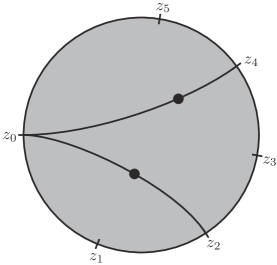
Figure 1. An element of $\mathcal{R}^{6,\{2,4\}}$

For any tuple ${\bf w}=(w_{0},w_{1},\dots,w_{k})$ of integers such that

$$w_{0}=w_{1}+\dots+w_{k}+|F|,$$ (2.11)

we consider the moduli $\mathcal{R}^{k+1,F,{\bf w}}$ of weighted popsicles, which is a copy of $\mathcal{R}^{k+1,F}$.

Recall further that the moduli spaces $\mathcal{R}^{k+1,F}$ admit compactifications obtained by adding broken stable popsicles as argued in [AS10b, Section 2.3 and Section 2.4]. Namely, we have

$$\overline{\mathcal{R}}^{k+1,F}=\bigsqcup_{(T,\mathbb{F})}\mathcal{R}^{T,\mathbb{F}},$$

where the sum runs over pairs $(T,\mathbb{F})$ of a rooted ribbon tree $T$ with $k+1$ semi-infinite ends and a decomposition $\mathbb{F}=\{F_{v}\}_{v:\text{vertex of }T}$ of $F$ such that the pair $(T,\mathbb{F})$ defines a stable broken popsicle. Moreover, for any such a pair $(T,\mathbb{F})$, there is an open set $\mathcal{U}^{T,\mathbb{F}}\subset\mathcal{R}^{T,\mathbb{F}}\times\prod_{e}(-1,0]$ and a gluing map

$$\mathcal{U}^{T,\mathbb{F}}\xrightarrow{\mathrm{glue}^{T,\mathbb{F}}}\overline{\mathcal{R}}^{k+1,F}$$

identifying

$$\mathcal{R}^{T,\mathbb{F}}\times\prod_{e}\{0\}\xrightarrow{\simeq}\mathcal{R}^{T,\mathbb{F}}\subset\overline{\mathcal{R}}^{k+1,F}.$$

There is a universal and consistent choice of strip-like ends $\{\epsilon_{m}=\epsilon_{m}^{P}\}_{P\in\mathcal{R}^{k+1,F}}$ for all pair $(k+1,{F})$. Here $\epsilon_{0}^{P}$ denotes the unique negative strip-like end on the popsicle $P$ and $\epsilon_{m}^{P}$ denotes the $m$-th positive strip-like end for $m=1,\dots,k$.

Now we consider Floer data for $\mathcal{R}^{k+1,F,{\bf w}}$. For the following definition of Floer data with Lagrangian labels, note that the moduli $\mathcal{R}^{2,\{1\}}$ has a unique element $P_{w}=(S_{0},\phi_{0})$ and hence so does $\mathcal{R}^{2,\{1\},(w+1,w)}$ for any integer $w$. Here $S_{0}$ is the infinite strip $\mathbb{R}\times[0,1]$.

Definition 2.6 (Floer data with Lagrangian labels).

Let Floer data associated to Lagrangian pairs be given as in Definition 2.1.

1. For any integer $w$, a Floer datum with Lagrangian labels on $\mathcal{R}^{2,\{1\},(w+1,w)}=\{P_{w}\}$, which is compatible with the chosen Floer data associated to Lagrangian pairs, consists of

   • a pair $(L_{0},L_{1})$ of admissible Lagrangians,

   • a domain-dependent Hamiltonian $H^{P_{w}}$ on $M$ and

   • a domain-dependent almost complex structure $I^{P_{w}}$

   such that

   1. $H^{P_{w}}_{(s,t)}$ is admissible for all $(s,t)\in\mathbb{R}\times[0,1]$,

   2. $H^{P_{w}}_{(s,t)}$ is independent of $t\in[0,1]$,

   3. $H^{P_{w}}_{(s,t)}=\begin{cases}H_{\tau^{(L_{0},L_{1})}_{w+1}}&(s\leq-1),\\ H_{\tau^{(L_{0},L_{1})}_{w}}&(s\geq 1),\end{cases}$

   4. $\partial_{s}H^{P_{w}}_{(s,t)}\leq 0$,

   5. $I^{P_{w}}_{(s,t)}\in\mathcal{J}(M)$ for all $(s,t)\in\mathbb{R}\times[0,1]$, and

   6. $I^{P_{w}}_{(s,t)}=\begin{cases}J^{(L_{0},L_{1})}_{w+1}(t)&(s\leq-1),\\ J^{(L_{0},L_{1})}_{w}(t)&(s\geq 1),\end{cases}$

   where

   $$\mathcal{J}(M)=\{J\,|\,J\text{ is an }\omega\text{-compatible complex structure of contact type on }\widehat{M}\}.$$

2. For any $k\in\mathbb{Z}_{\geq 1}$, a flavor $F\subseteq\{1,\dots,k\}$ and a tuple ${\bf w}=(w_{0},w_{1},\dots,w_{k})$ of integers satisfying (2.11), Floer data with Lagrangian labels on $\mathcal{R}^{k+1,F,{\bf w}}$, which is compatible with the chosen Floer data associated to Lagrangian pairs, consists of

   • a tuple $(L_{0},L_{1},\dots,L_{k})$ of admissible Lagrangians,

   • a smooth family $\{H^{P}\}_{P=(S,\phi)\in\mathcal{R}^{k+1,F,{\bf w}}}$ of domain-dependent Hamiltonians,

   • a smooth family $\{I^{P}\}_{P=(S,\phi)\in\mathcal{R}^{k+1,F,{\bf w}}}$ of domain-dependent almost complex structures and

   • a smooth family $\{\beta^{P}\}_{P=(S,\phi)\in\mathcal{R}^{k+1,F,{\bf w}}}$ of a 1-form $\beta\in\Omega^{1}(S)$

   such that

   1. $H^{P}_{z}$ is admissible for all $z\in S$,

   2. $H^{P}_{\epsilon_{j}(s,t)}=H_{\tau^{L_{j-1},L_{j}}_{w_{j}}}$ for $j=0,1,\dots,k$,

   3. $\beta^{P}|_{\partial S}=0$,

   4. $\epsilon_{j}^{*}\beta^{P}=dt$, for $j=0,1,\dots,k$,

   5. there exists a sufficiently large $R>0$, which is independent of $P\in\mathcal{R}^{k+1,F,{\bf w}}$,

      $$d_{S}(H^{P}_{z}\beta^{P})\leq 0$$ (2.12)

      for all $z\in[R,\infty)\times\partial M\subset\widehat{M}$, where $d_{S}$ is the differential with respect to the domain $S$,

   6. $I^{P}_{z}\in\mathcal{J}(M)$ for all $z\in S$, and

   7. $I^{P}_{\epsilon_{j}(s,t)}=J^{L_{j-1},L_{j}}_{w_{j}}(t)$ for $j=0,1,\dots,k$.

Remark 2.7.

1. Although the first content (1) of Definition 2.6 can be regarded as a special case of (2), we state it here separately since the Floer data discussed in (1) are those used to define the continuation maps.

2. The condition $\tau_{w}+\tau_{v}\leq\tau_{w+v}$, $w,v\in\mathbb{Z}$ is necessary to ensure that the conditions (b) and (e) of (2) in Definition 2.6 are compatible for $F=\emptyset$.

One may notice that our Floer data are different from those in [AS10b] in that we choose a family of Hamiltonians rather than choosing basic 1-forms and sub-closed 1-forms as a part of Floer data. Even so, a standard argument can be applied to showing that the above Floer data can be chosen in a consistent way in the sense that it is compatible with gluing maps in the sense discussed in [Sei08, Section (9i)]. Indeed we have:

Theorem 2.8.

There exists a universal and consistent choice of Floer data with Lagrangian labels on $\mathcal{R}^{k+1,F,{\bf w}}$ for all $k\geq 1$, all flavors $F$ and all weights ${\bf w}$ satisfying (2.11), which is compatible with given Floer data associated to Lagrangian pairs.

Let us fix universal and consistent Floer data with Lagrangian labels on $\mathcal{R}^{k+1,F,{\bf w}}$ for all Lagrangian labels and for all pairs $(k,F,{\bf w})$ of a flavor $F$ and a weight ${\bf w}=(w_{0},\dots,w_{k})$ satisfying (2.11), which are compatible with the Floer data associated to pairs of admissible Lagrangians chosen above.

Still, to ensure the transversality of the space of popsicle maps we will discuss below, one further needs an infinitesimal deformation of the almost complex structures $\{I^{P}\}_{P\in\mathcal{R}^{k+1,F,{\bf w}}}$ given as a part of the Floer data chosen above. Indeed, we need a family $\{K^{P}\}_{P\in\mathcal{R}^{k+1,F,{\bf w}}}$ of tangent vectors $K^{P}_{z}\in T_{I^{P}_{z}}\mathcal{J}(M)$, for which $K^{P}$ and its derivatives vanish on the strip-like ends of the popsicle $P$ for all popsicles $P$. For such an infinitesimal deformation, we get another family $\{J^{P}\}_{P\in\mathcal{R}^{k+1,F,{\bf w}}}$ of almost complex structures obtained by taking the exponential of $K^{P}$ at $I^{P}$. We refer the readers to [Sei08, Section (9k)] or [AS10b, Section 3.2] for more details.

Let us fix such an infinitesimal deformation $\{K^{P}\}_{P\in\mathcal{R}^{k+1,F,{\bf w}}}$ of almost complex structures. First, for some integer $w$ and a pair $(L_{0},L_{1})$ of admissible Lagrangians, let

$$x_{0}\in\mathcal{I}(L_{0},L_{1};H_{\tau_{w+1}})\text{ and }x_{1}\in\mathcal{I}(L_{0},L_{1};H_{\tau_{w}}).$$

be Hamiltonian chords and let us consider the space of stable popsicle maps

$$\mathcal{R}^{2,\{1\},(w+1,w)}(x_{0},x_{1})=\{u:\mathbb{R}\times[0,1]\to\widehat{M}\,|\,u\text{ satisfies }\mathrm{(i)},\mathrm{(ii)},\mathrm{(iii)}\text{ and }\mathrm{(iv)}\text{ below}\}$$ (2.13)

1. $u(s,j)\in\widehat{L}_{j}$ for all $s\in\mathbb{R}$ and for $j=0,1$.

2. $\lim_{s\to-\infty}u(s,t)=x_{0}(t)$.

3. $\lim_{s\to\infty}u(s,t)=x_{1}(t)$.

4. $\partial_{s}u+J^{P_{w}}(\partial_{t}u-X_{H^{P_{w}}}(u))=0$.

This space is used to define continuations $c_{w,w+1}$ as in (2.15).

For more general cases, note that, for each $P=(S,\phi)\in\mathcal{R}^{k+1,F,{\bf w}}$, the boundary $\partial S$ has $(k+1)$-components. We will denote by $\partial_{m}S$ the component between $m$-th and $(m+1)$-th boundary punctures of $\partial S$ for $m=0,\dots,k$. For an integer $k\in\mathbb{Z}_{\geq 1}$, a tuple $(L_{0},\dots,L_{k})$ of admissible Lagrangians and for some flavor $F\subseteq\{1,\dots,k\}$ and a weight ${\bf w}=(w_{0},w_{1},\dots,w_{k})$ satisfying $\eqref{eq:weight}$, let

$$x_{0}\in\mathcal{I}(L_{0},L_{k};H_{\tau_{w_{0}}}),x_{1}\in\mathcal{I}(L_{0},L_{1};H_{\tau_{w_{1}}}),\dots,\text{ and }x_{k}\in\mathcal{I}(L_{k-1},L_{k};H_{\tau_{w_{k}}})$$

be Hamiltonian chords. Then we consider the space of stable popsicle maps

$$\mathcal{R}^{k+1,F,{\bf w}}(x_{0},\dots,x_{k})=\{(P,u)\,|\,P=(S,\phi)\in\mathcal{R}^{k+1,F,{\bf w}},u:S\to\widehat{M}\text{ satisfies }\mathrm{(i)},\mathrm{(ii)},\mathrm{(iii)}\text{ and }\mathrm{(iv)}\text{ below}\}$$

1. $u(\partial_{m}S)\subset\widehat{L}_{m}$ for $m=0,1,\dots,k$.

2. $\lim_{s\to-\infty}u(\epsilon_{0}(s,t))=x_{0}(t)$.

3. $\lim_{s\to\infty}u(\epsilon_{m}(s,t))=x_{m}(t)$ for $m=1,\dots,k$.

4. $(du-X_{H^{P}_{u}}\otimes\beta)\circ j+J^{P}(du-X_{H^{P}_{u}}\otimes\beta)=0$, where $j$ is the complex structure on $S$.

Remark 2.9.

Following the manner we defined the space of popsicle maps above, the space $\mathcal{M}(x_{0},x_{1};H_{\tau_{w}},J_{w})$ of Floer strips defined in (2.2) can be written as $\mathcal{R}^{2,\emptyset,(w,w)}(x_{0},x_{1})$.

Since the condition (2.12) guarantees that popsicle maps with fixed inputs and outputs do not escape to infinity, we have the following as in [AS10b, Theorem 3.5].

Theorem 2.10.

Let $(k+1,F,{\bf w})$ be a tuple of an integer $k\in\mathbb{Z}_{\geq 1}$, a flavor $F\subseteq\{1,\dots,k\}$ and a weight ${\bf w}$ satisfying $k+|F|\geq 2$ and (2.11). For any tuple $(L_{0},\dots,L_{k})$ of admissible Lagrangians and Hamiltonian chords $x_{0},\dots,x_{k}$ given as above, we have

1. The spaces $\mathcal{R}^{k+1,F,{\bf w}}(x_{0},x_{1},\dots,x_{k})$ are smooth manifolds of expected dimensions

   $$k-2+|F|+\deg x_{0}-\sum_{i=1}^{k}\deg x_{i},$$ (2.14)

   for a generic choice of infinitesimal deformations $\{K^{P}\}_{P\in\mathcal{R}^{k+1,F,{\bf w}}}$.

2. The spaces $\mathcal{R}^{k+1,F,{\bf w}}(x_{0},x_{1},\dots,x_{k})$ admit compactifications obtained by adding broken stable popsicle maps and semi-stable popsicle maps.

After choosing such an infinitesimal deformation, for any tuple $(x_{0},x_{1},\dots,x_{k})$ of Hamiltonian chords such that the dimension (2.14) of $\mathcal{R}^{k+1,F,{\bf w}}(x_{0},\dots,x_{k})$ is zero, one gets a preferred isomorphism

$$|o_{(P,u)}|:|o_{x_{k}}|_{\mathbb{K}}\otimes\dots\otimes|o_{x_{1}}|_{\mathbb{K}}\to|o_{x_{0}}|_{\mathbb{K}}$$

for every element $(P,u)\in\mathcal{R}^{k+1,F,{\bf w}}(x_{0},x_{1},\dots,x_{k})$. We define the linear map

$$m^{k,F,{\bf w}}(x_{0},x_{1},\dots,x_{k})=\sum_{(P,u)\in\mathcal{R}^{k+1,F,{\bf w}}(x_{0},x_{1},\dots,x_{k})}|o_{(P,u)}|:|o_{x_{k}}|_{\mathbb{K}}\otimes\dots\otimes|o_{x_{1}}|_{\mathbb{K}}\to|o_{x_{0}}|_{\mathbb{K}}$$

as in [AS10b, Section 3.6].

In particular, the continuation map $c_{\tau_{w},\tau_{w+1}}:CF^{*}(L_{0},L_{1};H_{\tau_{w}})\to CF^{*}(L_{0},L_{1};H_{\tau_{w+1}})$ is defined by

$$c_{\tau_{w},\tau_{w+1}}=m^{1,\{1\},(w+1,w)}.$$ (2.15)

Now we are ready to construct products

$$\widecheck{\mu}^{k}:RFC^{*}(L_{k-1},L_{k})\otimes\dots\otimes RFC^{*}(L_{0},L_{1})\to RFC^{*}(L_{0},L_{k})[2-k]$$ (2.16)

for a given tuple $(L_{0},\dots,L_{k})$ of admissible Lagrangians of $M$.

For that purpose, let us first consider the identifications

$$CW_{n-*}(L_{0},L_{1})=A^{*}_{\leq 0}\oplus(B_{\leq 0}[-1])^{*}$$

for

$$A^{*}_{\leq 0}=\prod_{w=0}^{\infty}CF^{*}(L_{0},L_{1};H_{\tau_{-w}})\text{ and }B^{*}_{\leq 0}=\prod_{w=0}^{\infty}CF^{*}(L_{0},L_{1};H_{\tau_{-w}})$$

and

$$CW^{*}(L_{0},L_{1})=(A_{>0}[1])^{*}\oplus B^{*}_{>0}$$ (2.17)

for

$$A^{*}_{>0}=\bigoplus_{w=1}^{\infty}CF^{*}(L_{0},L_{1};H_{\tau_{w}})\text{ and }B^{*}_{>0}=\bigoplus_{w=1}^{\infty}CF^{*}(L_{0},L_{1};H_{\tau_{w}})$$

as graded vector spaces.

Consequently, as a graded vector space, we have the following identifications:

$$RFC^{*}(L_{0},L_{1}) =CW_{n-*}(L_{0},L_{1})[1]\oplus CW^{*}(L_{0},L_{1})$$

$$=(A_{\leq 0}[1])^{*}\oplus B_{\leq 0}^{*}\oplus(A_{>0}[1])^{*}\oplus B_{>0}^{*}$$

$$=A[1]^{*}\oplus B^{*}$$

for

$$A^{*}=A_{\leq 0}^{*}\oplus A_{>0}^{*}\text{ and }B^{*}=B_{\leq 0}^{*}\oplus B_{>0}^{*}.$$

Or equivalently, one may think of this as the formal variables $q$ and $q^{\vee}$ cancel each other so that

$$CW_{n-*}(L_{0},L_{1})[1]=CW_{n-1-*}(L_{0},L_{1})q=(A^{*+1}_{\leq 0}\oplus B^{*}_{\leq 0}q^{\vee})q=A^{*+1}_{\leq 0}q\oplus B^{*}_{\leq 0}$$

and hence

$$RFC^{*}(L_{0},L_{1}) =CW_{n-1-*}(L_{0},L_{1})q\oplus CW^{*}(L_{0},L_{1})$$

$$=(A^{*+1}_{\leq 0}q\oplus B^{*}_{\leq 0})\oplus(A^{*+1}_{>0}q\oplus B^{*}_{>0})$$

$$=A^{*+1}q\oplus B^{*}.$$

Here $A^{*}$ and $B^{*}$ can be described as follows:

$$A^{*}=B^{*}=\left\{(x_{w})_{w}\in\prod_{w\in\mathbb{Z}}CF^{*}(L_{0},L_{1};H_{\tau_{w}})\,\Big{|}\,\exists\text{ only finitely many }w>0\text{ such that }x_{w}\neq 0\right\}.$$ (2.18)

Now, let $(k,F,{\bf w})$ be a triple given as in Theorem 2.10. Then let exponents $j_{m}\in\{0,1\}$ be determined by

$$j_{m}=\begin{cases}1&(m\in F),\\ 0&(\text{otherwise})\end{cases}$$

for $m\in\{1,\dots,k\}$. We define an operator

$$\mu^{k,F,{\bf w}}_{B}:CF^{*}(L_{i_{k-1}},L_{i_{k}};H_{\tau_{w_{k}}})q^{j_{k}}\otimes\dots\otimes CF^{*}(L_{i_{0}},L_{i_{1}};H_{\tau_{w_{1}}})q^{j_{1}}\to CF^{*}(L_{i_{0}},L_{i_{k}};H_{\tau_{w_{0}}}),$$

of degree $2-k$ by mapping

$$x_{k}q^{j_{k}}\otimes\dots\otimes x_{1}q^{j_{1}}\mapsto\sum_{x_{0}\in\mathcal{I}(L_{i_{0}},L_{i_{k}};H_{\tau_{w_{0}}})}(-1)^{*}m^{k,F,{\bf w}}(x_{0},\dots,x_{k})(x_{k}\otimes\dots\otimes x_{1}),$$

for $x_{j}\in\mathcal{I}(L_{i_{j-1}},L_{i_{j}};H_{\tau_{w_{j}}})$ and $*=\sum_{j}\deg x_{j}+\sum_{j\in F}\sum_{m>j}(\deg x_{m}-1)$, and extending this linearly.

Next, for each $m\in F$, consider

$$F^{m}=F\setminus\{m\}$$

and

$${\bf w}^{m}=(w_{0}-1,w_{1},\dots,w_{k}).$$

Then, we define an operator

$$\mu^{k,F,{\bf w}}_{A}:CF^{*}(L_{i_{k-1}},L_{i_{k}};H_{\tau_{w_{k}}})q^{j_{m}}\otimes\dots\otimes CF^{*}(L_{i_{0}},L_{i_{1}};H_{\tau_{w_{1}}})q^{j_{1}}\to CF^{*}(L_{i_{0}},L_{i_{k}};H_{\tau_{w_{0}-1}})$$

of degree $3-k$ by mapping

$$x_{k}q^{j_{k}}\otimes\dots\otimes x_{m}q^{j_{m}}\otimes\dots\otimes x_{1}q^{j_{1}}\mapsto\sum_{m\in F}(-1)^{*_{m}}\mu^{k,F^{m},{\bf w}^{m}}_{B}(x_{k}q^{j_{k}}\otimes\dots\otimes x_{m}\otimes\dots x_{1}q^{j_{1}}),$$

for $x_{j}\in\mathcal{I}(L_{i_{j-1}},L_{i_{j}};H_{\tau_{w_{j}}})$ and

$$*_{m}=\sum_{l=m+1}^{k}(\deg x_{l}+1),$$

and extending this linearly.

Having done this, we define the product $\widecheck{\mu}^{k}$ (2.16) by

$$\begin{split}\widecheck{\mu}^{k}\left((x^{k}_{w_{k}})_{w_{k}}q^{j_{k}},\dots,(x^{1}_{w_{1}})_{w_{1}}q^{j_{1}}\right)=&\left(\sum_{\sum_{i=1}^{k}w_{i}+|F|-1=w_{0}}\mu^{k,F,(\sum w_{i}+|F|,w_{k},\dots,w_{1})}_{A}(x^{k}_{w_{k}}q^{j_{k}}\otimes\dots\otimes x^{1}_{w_{1}}q^{j_{1}})\right)_{w_{0}}q\\ &+\left(\sum_{\sum_{i=1}^{k}w_{i}+|F|=w_{0}}\mu^{k,F,(\sum w_{i}+|F|,w_{k},\dots,w_{1})}_{B}(x^{k}_{w_{k}}q^{j_{k}}\otimes\dots\otimes x^{1}_{w_{1}}q^{j_{1}})\right)_{w_{0}},\end{split}$$ (2.19)

for any

$$(x_{w_{m}}^{m})_{w_{m}}q^{j_{m}}\in\begin{cases}B^{*}&(j_{m}=0),\\ A^{*+1}q&(j_{m}=1),\end{cases}$$

for $m=1,\dots,k$.

Then we finally have the following theorem.

Theorem 2.11 (cf. [GGV22, Lemma 4.9 and Lemma 4.11]).

There exist products $\widecheck{\mu}^{k}$ on Rabinowitz Floer complexes such that

1. $\widecheck{\mu}^{k}$ satisfy the $A_{\infty}$-relation.

2. The natural inclusions $i:CW^{*}(L_{i},L_{j})\hookrightarrow RFC^{*}(L_{i},L_{j})$ induce an $A_{\infty}$-homomorphism

   $$\bigoplus_{i,j}CW^{*}(L_{i},L_{j})\to\bigoplus_{i,j}RFC^{*}(L_{i},L_{j})$$

   for any collection $\{L_{i}\}$ of admissible Lagrangians. In particular, the inclusions induce an $A_{\infty}$-functor from the wrapped Fukaya category $\mathcal{W}(M)$ to the Rabinowitz Fukaya category $\mathcal{RW}(M)$.

Proof.

For the first statement, from the description of $A^{*}$ and $B^{*}$ in (2.18), one can deduce that every summand of $\widecheck{\mu}^{k}$ in (2.19) is a finite sum. This guarantees that those two operators are well-defined. Then essentially the same argument proving [AS10b, Proposition 3.15] can be applied to showing that $\widecheck{\mu}^{k}$ satisfy the $A_{\infty}$-relation.

For the second statement, first observe from (2.17) that the image of the inclusion $CW^{*}(L_{i},L_{j})\to RFC^{*}(L_{i},L_{j})$ coincides with $A^{*+1}_{>0}q\oplus B^{*}_{>0}$. But from the construction (2.19) one can deduce that if

$$(x_{w}^{m})_{w}q^{j_{m}}\in\begin{cases}A^{*+1}_{>0}q&(j_{m}=1),\\ B^{*}_{>0}&(j_{m}=0)\end{cases}$$

for all $1\leq m\leq k$, then the product $\widecheck{\mu}^{k}((x^{k}_{w})_{w}q^{j_{k}}\otimes\dots\otimes(x^{1}_{w})_{w}q^{j_{1}})$ lies in $A^{*+1}_{>0}q\oplus B^{*}_{>0}$ again. Furthermore, when restricted to the image of the inclusion $CW^{*}(L_{0},L_{1})\to RFC^{*}(L_{0},L_{1})$, the higher product $\widecheck{\mu}^{k}$ coincides with the higher product $\mu^{k}$ constructed in [AS10b] as a part of the $A_{\infty}$-structure on wrapped Floer complexes. These observations prove the assertion. ∎

3. Calabi–Yau property of derived Rabinowitz Fukaya category

The main goal of this section is to prove that the derived Rabinowitz Fukaya category of a Liouville domain $M$ of dimension $2n$ is $(n-1)$-Calabi–Yau assuming the condition (3) of Theorem 1.2.

To prove the assertion, we first show that there is a non-degenerate paring

$$\beta^{k}=\beta^{k}_{L_{i},L_{j}}:RFH^{n-1-k}(L_{j},L_{i})\times RFH^{k}(L_{i},L_{j})\to\mathbb{K},$$

for any pair $i,j\in I$ and any $k\in\mathbb{Z}$. We further show that this non-degenerate pairing can be extended to the triangulated envelope of the Rabinowitz Fukaya category.

Note that, for a given chain complex $C$ over a field $\mathbb{K}$, we denote its dual complex $\mathrm{Hom}_{\mathbb{K}}(C,\mathbb{K})$ by $C^{\vee}$. Then our strategy to show the existence of a non-degenerate pairing $\beta$ is to construct chain maps

• $\overline{\alpha}:CW^{*}(L_{i},L_{j})\to CW_{*}(L_{j},L_{i})^{\vee}$,

• $\overline{\gamma}:CW_{n-1-*}(L_{i},L_{j})\to(CW^{n-1-*}(L_{j},L_{i}))^{\vee}$ and

• $\overline{\beta}:RFC^{*}(L_{i},L_{j})\to(RFC^{n-1-*}(L_{j},L_{i}))^{\vee}$

for $i,j\in I$ such that the following diagram commutes:

(3.1)

We will further show that $\overline{\alpha}$ is a quasi-isomorphism if the condition (3) of Theorem 1.2 is satisfied and $\overline{\gamma}$ is a quasi-isomorphism even without such an assumption. Then the commutativity of the above diagram and the five-lemma imply that $\overline{\beta}$ is a quasi-isomoprhism as well. Since taking dual and taking homology commute over a field, we have

$$RFH^{n-1-*}(L_{j},L_{i})^{\vee}=H^{*}(RFC^{n-1-*}(L_{j},L_{i})^{\vee}).$$

This implies that the pairing

$$\beta^{k}:RFH^{n-1-k}(L_{j},L_{i})\times RFH^{k}(L_{i},L_{j})\to\mathbb{K},k\in\mathbb{Z}$$

defined by

$$\beta^{k}([y],[x])=\overline{\beta}(x)(y)$$

for all cycles $x\in RFC^{k}(L_{i},L_{j})$ and $y\in RFC^{n-1-k}(L_{j},L_{i})$ is non-degenerate.

3.1. Construction of $\overline{\alpha}$ and $\overline{\gamma}$

Let us begin the construction of the chain maps $\overline{\alpha}$ and $\overline{\gamma}$. First, for any admissible Lagrangian $L$ of $M$, let $\epsilon_{L}>0$ be sufficiently small so that

$$\epsilon_{L}<\mathrm{min}~{}\mathrm{Spec}(\partial L,\partial L)\cap\mathbb{R}_{>0}.$$

We may assume that the Floer data $\{(\tau^{L_{0},L_{1}}_{w},H_{\tau^{L_{0},L_{1}}_{w}},J^{L_{0},L_{1}}_{w})\}_{w\in\mathbb{Z}}$ associated to Lagrangian pairs (Definition 2.1) have been chosen in such a way that the following three additional conditions are satisfied:

1. $-\epsilon_{L}<\tau^{L,L}_{0}<0<\tau^{L,L}_{1}<\epsilon_{L}$ for all admissible Lagrangian $L$.

2. $-\epsilon_{L_{0}}<\tau_{w}^{L_{0},L_{1}}+\tau_{-w}^{L_{1},L_{0}}(\leq\tau_{0}^{L_{0},L_{0}}$) for all $w\in\mathbb{Z}$ and all admissible Lagrangians $L_{0}$ and $L_{1}$.

3. $H_{\tau^{L,L}_{0}}|_{L}$ and $H_{\tau^{L,L}_{1}}|_{L}$ are $C^{2}$-small Morse functions for any admissible Lagrangian $L$.

Denoting $\tau^{L,L}_{w}$ by $\tau_{w}$ for $w\in\mathbb{Z}$, the Floer complex $CF^{*}(L,L;H_{\tau_{0}})$ (respectively $CF^{*}(L,L;H_{\tau_{1}})$) can be identified with the cohomological Morse complex $CM^{*}(L;H_{\tau_{0}}|_{L})$ (respectively $CM^{*}(L;H_{\tau_{1}}|_{L})$), as argued in [CO18, Proposition 2.10] and [Rit13, Section 5].

Furthermore, the Morse complex $CM^{*}(L;H_{\tau_{0}}|_{L})$ is canonically identified with the dual of the Morse complex $CM^{n-*}(L;-H_{\tau_{0}}|_{L})$ by definition. Namely, there is an identification:

$$CM^{*}(L;H_{\tau_{0}}|_{L})^{\vee}=CM^{n-*}(L;-H_{\tau_{0}}|_{L}).$$

But, the homology of the latter $CM^{n-*}(L;-H_{\tau_{0}}|_{L})$ is isomorphic to $H^{n-*}(L;\mathbb{K})$ or $H_{*}(L,\partial L;\mathbb{K})$ as $-H_{\tau_{0}}|_{L}$ has a positive slope less than $\epsilon_{L}$ at infinity. Consequently, the homology of $CM^{*}(L;H_{\tau_{0}}|_{L})$ is isomorphic to $H^{*}(L,\partial L;\mathbb{K})$ or $H_{n-*}(L;\mathbb{K})$.

Let $\psi_{L}\in CM^{n}(L;H_{\tau_{0}}|_{L})^{\vee}=CM^{0}(L;-H_{\tau_{0}}|_{L})$ be a cycle that represents the unit class $1\in H^{0}(L;\mathbb{K})$ or the relative fundamental class $[L,\partial L]\in H_{n}(L,\partial L;\mathbb{K})$. Equipping the ground field $\mathbb{K}$ with the trivial differential, this gives rise to a chain map $\langle[L,\partial L],-\rangle:CM^{*}(L;H_{\tau_{0}}|_{L})\to\mathbb{K}$ defined by

$$\langle[L,\partial L],x\rangle=\psi_{L}(x).$$

Now we are ready to define chain maps

$$\begin{split}\alpha&=\alpha_{L_{0},L_{1}}:CW_{*}(L_{1},L_{0})\otimes CW^{*}(L_{0},L_{1})\to\mathbb{K},\\ \gamma&=\gamma_{L_{0},L_{1}}:CW^{*}(L_{1},L_{0})\otimes CW_{*}(L_{0},L_{1})\to\mathbb{K}.\end{split}$$

Here we equip the tensor product $CW_{*}(L_{1},L_{0})\otimes CW^{*}(L_{0},L_{1})$ with the differential $\delta^{\prime}$ given by

$$\delta^{\prime}(y\otimes x)=\left((-1)^{\deg x}\partial(y)\otimes x+y\otimes\delta(x)\right)$$

for all homogeneous elements $x\in CW^{*}(L_{0},L_{1})$ and $y\in CW_{*}(L_{1},L_{0})$ and equip the tensor product $CW^{*}(L_{1},L_{0})\otimes CW_{*}(L_{0},L_{1})$ with a differential defined similarly.

Recall from (2.10) that there exist the inclusion map

$$i:CW^{*}(L_{0},L_{1})\to RFC^{*}(L_{0},L_{1})$$

and the quotient map

$$p:RFC^{*}(L_{0},L_{1})\to CW_{n-1-*}(L_{0},L_{1}),$$

which are chain maps. Even though there is no chain map from $CW_{n-1-*}(L_{0},L_{1})$ to $RFC^{*}(L_{0},L_{1})$ that is the inverse of $p$, $CW_{n-1-*}(L_{0},L_{1})$ is still a subspace of $RFC^{*}(L_{0},L_{1})$. Let us denote the inclusion map by

$$p^{-1}:CW_{n-1-*}(L_{0},L_{1})\to RFC^{*}(L_{0},L_{1}),$$

which is also a right inverse of $p$.

We define the map $\alpha$ and $\gamma$

$$\alpha(y\otimes x) =\left\langle[L_{0},\partial L_{0}],\pi\circ p\circ\widecheck{\mu}^{2}(p^{-1}(y)\otimes i(x))\right\rangle,$$

$$\gamma(x\otimes y) =\left\langle[L_{0},\partial L_{0}],\pi\circ p\circ\widecheck{\mu}^{2}(i(x)\otimes p^{-1}(y))\right\rangle$$

for $y\in CW_{*}(L_{1},L_{0})$ and $x\in CW^{*}(L_{0},L_{1})$, where $\pi:CW_{n-*}(L_{0},L_{0})\to CF^{*}(L_{0},L_{0};H_{\tau_{0}})\cong CM^{*}(L_{0};H_{\tau_{0}}|_{L_{0}})$ is the projection map discussed in (2.8). Then we have:

Lemma 3.1.

Both $\alpha$ and $\gamma$ are chain maps.

Proof.

Let us prove the assertion for $\alpha$ only since the other one can be proved similarly. Since the operators $\langle[L_{0},\partial L_{0}],-\rangle$ and $\pi$ are already chain maps, it suffices to show that the map $\eta:CW_{*}(L_{1},L_{0})\otimes CW^{*}(L_{0},L_{1})\to CW_{*}(L_{0},L_{0})$ defined by

$$\eta(y\otimes x)=p\circ\widecheck{\mu}^{2}(p^{-1}(y)\otimes i(x))$$

is a chain map.

Let $\pi^{-1}:CF^{n-*}(L_{1},L_{0};H_{\tau_{0}})\to CW_{*}(L_{1},L_{0})$ be the inclusion map, which is also a right inverse of $\pi$. Then every element $y\in CW_{*}(L_{1},L_{0})$ is the sum

$$y=y^{\prime}+y^{\prime\prime}=(y-\pi^{-1}(\pi(y)))+\pi^{-1}(\pi(y))$$

of an element $y^{\prime}=y-\pi^{-1}(\pi(y))$ that does not involve any summand from $CF^{n-*}(L_{1},L_{0};H_{\tau_{0}})\subset A_{\leq 0}^{*}\subset CW_{*}(L_{1},L_{0})$ and an element $y^{\prime\prime}=\pi^{-1}(\pi(y))\in CF^{n-*}(L_{1},L_{0};H_{\tau_{0}})\subset CW_{*}(L_{1},L_{0})$. Hence it also suffices to show that the assertion holds for such elements $y^{\prime}$ and $y^{\prime\prime}$ separately.

Let us first show that the assertion holds for $y^{\prime}\otimes x$, for which $y^{\prime}$ does not involve any summand from $CF^{n-*}(L_{1},L_{0};H_{\tau_{0}})$. Indeed, for such elements $y^{\prime}$, one can observe

$$\widecheck{\mu}^{1}\circ p^{-1}(y^{\prime})=-p^{-1}\circ\partial(y^{\prime})$$

from the definition of the differential $\partial$ on $CW_{*}(L_{1},L_{0})$ and (2.9). Therefore, we have

$$\begin{split}\eta\circ\delta^{\prime}(y^{\prime}\otimes x)&=(-1)^{\deg x}\eta(\partial(y^{\prime})\otimes x)+\eta(y^{\prime}\otimes\delta(x))\\ &=(-1)^{\deg x}p\circ\widecheck{\mu}^{2}(p^{-1}\left(\partial(y^{\prime}))\otimes i(x)\right)+p\circ\widecheck{\mu}^{2}\left(p^{-1}(y^{\prime})\otimes\delta(i(x))\right)\\ &=(-1)^{\deg x-1}p\circ\widecheck{\mu}^{2}\left(\widecheck{\mu}^{1}(p^{-1}(y^{\prime}))\otimes i(x)\right)+p\circ\widecheck{\mu}^{2}\left(p^{-1}(y^{\prime})\otimes\widecheck{\mu}^{1}(i(x))\right)\\ &=p\left((-1)^{\deg x-1}\widecheck{\mu}^{2}\left(\widecheck{\mu}^{1}(p^{-1}(y^{\prime}))\otimes i(x)\right)+\widecheck{\mu}^{2}\left(p^{-1}(y^{\prime})\otimes\widecheck{\mu}^{1}(i(x))\right)\right)\\ &=-p\circ\widecheck{\mu}^{1}\circ\widecheck{\mu}^{2}\left(p^{-1}(y^{\prime})\otimes i(x)\right)\\ &=\partial\circ p\circ\widecheck{\mu}^{2}\left(p^{-1}(y^{\prime})\otimes i(x)\right)\\ &=\partial\circ\eta(y^{\prime}\otimes x).\end{split}$$ (3.2)

This proves the assertion.

Now, for all homogeneous elements $y^{\prime\prime}\in CF^{n-1-*}(L_{1},L_{0};H_{\tau_{0}})\subset CW_{*}(L_{1},L_{0})$, observe

$$\widecheck{\mu}^{1}\circ p^{-1}(y^{\prime\prime})=-p^{-1}\circ\partial(y^{\prime\prime})+(-1)^{\deg y^{\prime\prime}+1}i\circ c_{\tau_{0},\tau_{1}}(y^{\prime\prime}),$$

where $i\circ c_{\tau_{0},\tau_{1}}:CF^{n-1-*}(L_{1},L_{0};H_{\tau_{0}})\to RFC^{n-1-*}(L_{1},L_{0})$ factors through

$$CF^{n-1-*}(L_{1},L_{0};H_{\tau_{0}})\xrightarrow{c_{\tau_{0},\tau_{1}}}CF^{n-1-*}(L_{1},L_{0};H_{\tau_{1}})\subset CW^{n-1-*}(L_{1},L_{0})\xrightarrow{i}RFC^{n-1-*}(L_{1},L_{0}).$$

The above argument (3.2) can be applied here with only difference that a multiple of the following term

$$p\circ\widecheck{\mu}^{2}\left(i(c_{\tau_{0},\tau_{1}}(y^{\prime\prime}))\otimes i(x)\right)$$

is added to the lines following from the third line in (3.2). But the above term is zero since the inclusion $i$ induces an $A_{\infty}$-homomorphism as argued in Theorem 2.11 and hence the above term equals

$$0=p\circ i\circ\mu^{2}(c_{\tau_{0},\tau_{1}}(y^{\prime\prime})\otimes x).$$

This completes the proof. ∎

As a consequence of Lemma 3.1, $\alpha$ and $\gamma$ induce the pairings

$$\alpha^{k}:HW_{k}(L_{1},L_{0})\times HW^{k}(L_{0},L_{1}) \to\mathbb{K},$$

$$\gamma^{k}:HW^{k}(L_{1},L_{0})\times HW_{k}(L_{0},L_{1}) \to\mathbb{K}$$

for each $k\in\mathbb{Z}$.

Furthermore, Lemma 3.1 allows us to consider the following chain maps:

$$\overline{\alpha}:CW^{*}(L_{0},L_{1})\to CW_{*}(L_{1},L_{0})^{\vee}\text{ and }\overline{\gamma}:CW_{*}(L_{0},L_{1})\to CW^{*}(L_{1},L_{0})^{\vee}$$

defined by

$$\overline{\alpha}(x)(y) =\alpha(y\otimes x),$$

$$\overline{\gamma}(y)(x) =\gamma(x\otimes y)$$

for all $x\in CW^{*}(L_{0},L_{1})$ and $y\in CW_{*}(L_{1},L_{0})$.

Let us denote their induced maps on homologies by

$$\begin{split}\overline{\alpha}^{k}&:HW^{k}(L_{0},L_{1})\to HW_{k}(L_{1},L_{0})^{\vee},\\ \overline{\gamma}^{k}&:HW_{k}(L_{0},L_{1})\to HW^{k}(L_{1},L_{0})^{\vee}\end{split}$$

for each $k\in\mathbb{Z}$.

Now let us turn into the proof that both $\overline{\alpha}$ and $\overline{\gamma}$ induce isomorphisms on homologies assuming that the condition (3) of Theorem 1.2 is satisfied. For that purpose, first observe that, for each $w\in\mathbb{Z}_{\geq 1}$, there are embeddings

$$CF^{*}(L_{0},L_{1};H_{\tau_{w}})\subset CW^{*}(L_{0},L_{1})\text{ and }CF^{n-*}(L_{1},L_{0};H_{\tau_{-w}})\subset CW_{*}(L_{1},L_{0})$$

as subspaces. This allows us to consider the restriction of the product $\widecheck{\mu}^{2}$ to $CF^{n-*}(L_{1},L_{0};H_{\tau_{-w}})\otimes CF^{*}(L_{0},L_{1};H_{\tau_{w}})$ given by

$${\mu}^{2,\emptyset,(0,w,-w)}_{B}:CF^{n-*}(L_{1},L_{0};H_{\tau_{-w}})\otimes CF^{*}(L_{0},L_{1};H_{\tau_{w}})\to CF^{n}(L_{0},L_{0};H_{\tau_{0}}).$$

But, for $x_{0}\in CF^{n}(L_{0},L_{0};H_{\tau_{0}})$, $x_{1}\in CF^{*}(L_{0},L_{1};H_{\tau_{w}})$ and $x_{2}\in CF^{n-*}(L_{1},L_{0};H_{\tau_{-w}})$, the space $\mathcal{R}^{3,\emptyset,(0,w,-w)}(x_{0},x_{1},x_{2})$ of popsicle maps coincides with the space of pair-of-pants curves with one negative end $x_{0}$ and two positive ends $x_{1}$ and $x_{2}$. Therefore $\mu^{2,\emptyset,(0,-w,w)}_{B}$ coincides with the pair-of-pants product up to sign.

Similarly, the product $\widecheck{\mu}^{2}$ restricts to

$$\mu^{2,\emptyset,(0,-w,w)}_{B}:CF^{n-1-*}(L_{1},L_{0};H_{\tau_{w}})\otimes CF^{*+1}(L_{0},L_{1};H_{\tau_{-w}})\to CF^{n}(L_{0},L_{0};H_{\tau_{0}}),$$

which also coincides with the pair-of-pants product up to sign. Let

$$\begin{split}\widetilde{\alpha}_{w}&:CF^{n-*}(L_{1},L_{0}:H_{\tau_{-w}})\otimes CF^{*}(L_{0},L_{1};H_{\tau_{w}})\to\mathbb{K},\\ \widetilde{\gamma}_{w}&:CF^{n-1-*}(L_{1},L_{0};H_{\tau_{w}})\otimes CF^{*+1}(L_{0},L_{1};H_{\tau_{-w}})\to\mathbb{K}\end{split}$$ (3.3)

be the chain maps defined by

$$\widetilde{\alpha}_{w}(y\otimes x) =\langle[L_{0},\partial L_{0}],\mu^{2,\emptyset,(0,w,-w)}_{B}(y\otimes x)\rangle,$$

$$\widetilde{\gamma}_{w}(x\otimes y) =\langle[L_{0},\partial L_{0}],\mu^{2,\emptyset,(0,-w,w)}_{B}(x\otimes y)\rangle.$$

Let us denote the induced pairings on homologies by

$$\widetilde{\alpha}^{k}_{w} :HF^{n-k}(L_{1},L_{0}:H_{\tau_{-w}})\times HF^{k}(L_{0},L_{1};H_{\tau_{w}})\to\mathbb{K},$$

$$\widetilde{\gamma}^{k}_{w} :HF^{k}(L_{1},L_{0};H_{\tau_{w}})\times HF^{n-k}(L_{0},L_{1};H_{\tau_{-w}})\to\mathbb{K}$$

for each $k\in\mathbb{Z}$ by abuse of notation.

Remark 3.2.

In general, these pairings $\widetilde{\alpha}_{w+1}^{k}$ and $\widetilde{\gamma}_{w+1}^{n-k}$ are not nondegenerate since $\tau_{-w}$ may not be close to $-\tau_{w}$ so that $[\tau_{-w},-\tau_{w}]\cap\mathrm{Spec}(\partial L_{1},\partial L_{0})\ \neq\emptyset$. This is the reason why we later choose other slopes $\sigma_{-w}$ in the proof of Lemma 3.3.

The pairings $\widetilde{\alpha}_{w+1}^{k}$ and $\widetilde{\gamma}_{w+1}^{n-k}$ are compatible with the continuations in the sense that

$$\begin{split}\widetilde{\alpha}_{w+1}^{k}(y,c_{w}(x))&=\widetilde{\alpha}_{w}^{k}(c_{-(w+1)}(y),x),\\ \widetilde{\gamma}_{w+1}^{n-k}(c_{w}(x),y)&=\widetilde{\gamma}_{w}^{n-k}(x,c_{-(w+1)}(y))\end{split}$$ (3.4)

for all $w\in\mathbb{Z}_{\geq 0}$, $k\in\mathbb{Z}$, $x\in HF^{k}(L_{0},L_{1};H_{\tau_{w}})$ and $y\in HF^{n-k}(L_{1},L_{0};H_{\tau_{-(w+1)}})$. This implies that these induce pairings on limits as follows.

$$\begin{split}\widetilde{\alpha}^{k}&:\varprojlim_{w\to\infty}HF^{n-k}(L_{1},L_{0};H_{\tau_{-w}})\times\varinjlim_{w\to\infty}HF^{k}(L_{0},L_{1};H_{\tau_{w}})\to\mathbb{K},\\ \widetilde{\gamma}^{k}&:\varinjlim_{w\to\infty}HF^{k}(L_{1},L_{0};H_{\tau_{w}})\times\varprojlim_{w\to\infty}HF^{n-k}(L_{1},L_{0};H_{\tau_{-w}})\to\mathbb{K}.\end{split}$$

Finally, these induce maps

$$\begin{split}\overline{\widetilde{\alpha}}^{k}&:\varinjlim_{w\to\infty}HF^{k}(L_{0},L_{1};H_{\tau_{w}})\to(\varprojlim_{w\to\infty}HF^{n-k}(L_{1},L_{0};H_{\tau_{-w}}))^{\vee},\\ \overline{\widetilde{\gamma}}^{k}&:\varprojlim_{w\to\infty}HF^{n-k}(L_{1},L_{0};H_{\tau_{-w}})\to(\varinjlim_{w\to\infty}HF^{k}(L_{1},L_{0};H_{\tau_{w}}))^{\vee}.\end{split}$$

Lemma 3.3.

1. For $k\in\mathbb{Z}$, if $\dim HW^{k}(L_{0},L_{1})=\dim\varinjlim_{w\to\infty}HF^{k}(L_{0},L_{1};H_{\tau_{w}})<\infty$, then $\overline{\widetilde{\alpha}}^{k}$ is an isomorphism.

2. For $k\in\mathbb{Z}$, $\overline{\widetilde{\gamma}}^{k}$ is an isomorphism.

Proof.

Let us prove the first assertion first. For each $w\in\mathbb{Z}_{\geq 1}$, we may choose $\sigma_{-w}\in\mathbb{R}$ in such a way that

• $\tau_{-w}\leq\sigma_{-w}\leq-\tau_{w}+\tau_{0}$,

• $[\sigma_{-w},-\tau_{w}]\cap\mathrm{Spec}(\partial L_{1},\partial L_{0})=\emptyset$.

Then the pairing $a^{k}_{w}:HF^{n-k}(L_{1},L_{0};H_{\sigma_{-w}})\times HF^{k}(L_{0},L_{1};H_{\tau_{w}})\to\mathbb{K}$ given as above is non-degenerate as proved in [CO20, Section 6.1]. This implies that there is an isomorphism

$$\overline{a}^{k}_{w}:HF^{k}(L_{0},L_{1};H_{\tau_{w}})\cong HF^{n-k}(L_{1},L_{0};H_{\sigma_{-w}})^{\vee},$$

which makes sense since both $HF^{*}(L_{0},L_{1};H_{\tau_{w}})$ and $HF^{n-*}(L_{1},L_{0};H_{\sigma_{-w}})$ are finite-dimensional.

Furthermore, $\sigma_{-w}$ can be chosen in such a way that the sequence $(\sigma_{-w})_{w\in\mathbb{Z}_{\geq 1}}$ is decreasing so that we may identify

$$\varprojlim_{w\to\infty}HF^{n-k}(L_{1},L_{0};H_{\tau_{-w}})=\varprojlim_{w\to\infty}HF^{n-k}(L_{1},L_{0};H_{\sigma_{-w}}).$$ (3.5)

Then since the isomorphisms $\overline{a}^{k}_{w}$ are compatible with continuations once again, we have

$$\overline{a}^{k}:\varinjlim_{w\to\infty}HF^{k}(L_{0},L_{1};H_{\tau_{w}})\to(\varprojlim_{w\to\infty}HF^{n-k}(L_{1},L_{0};H_{\sigma_{-w}}))^{\vee}.$$

Here note that the assumption $\dim\varinjlim_{w\to\infty}HF^{k}(L_{0},L_{1};H_{\tau_{w}})<\infty$ implies that

$$\begin{split}\varinjlim_{w\to\infty}HF^{k}(L_{0},L_{1};H_{\tau_{w}})&\cong\left((\varinjlim_{w\to\infty}HF^{k}(L_{0},L_{1};H_{\tau_{w}}))^{\vee}\right)^{\vee}\\ &\cong\left(\varprojlim_{w\to\infty}HF^{k}(L_{0},L_{1};H_{\tau_{w}})^{\vee}\right)^{\vee}.\end{split}$$

Since $HF^{n-k}(L_{1},L_{0};H_{\sigma_{-w}})$ is identified with $HF^{k}(L_{0},L_{1};H_{\tau_{w}})^{\vee}$ via $(\overline{a}_{w}^{k})^{\vee}$ for each $w$ and the dual of the continuation map $c_{\tau_{w},\tau_{w+1}}:HF^{k}(L_{0},L_{1};H_{\tau_{w}})\to HF^{k}(L_{0},L_{1};H_{\tau_{w+1}})$ is identified with the continuation map $c_{-\sigma_{w+1},-\sigma_{w}}$ under the identification $(\overline{a}_{w}^{k})^{\vee}$ due to a compatibility as in (3.4), this implies that

$$\varinjlim_{w\to\infty}HF^{k}(L_{0},L_{1};H_{\tau_{w}})\cong\left(\varprojlim_{w\to\infty}HF^{n-k}(L_{1},L_{0};H_{\sigma_{-w}})\right)^{\vee}.$$

Finally (3.5) proves the first assertion.

The second assertion can be proved similarly even without any assumption on dimension since the dual of a direct limit is given by the inverse limit of duals in general. ∎

Now we are ready to prove the following lemma.

Lemma 3.4.

1. For $k\in\mathbb{Z}$, if $\dim HW^{k}(L_{0},L_{1})<\infty$, $\overline{\alpha}^{k}:HW^{k}(L_{0},L_{1})\to HW_{k}(L_{1},L_{0})^{\vee}$ is an isomorphism.

2. For $k\in\mathbb{Z}$, $\overline{\gamma}^{k}:HW_{k}(L_{0},L_{1})\to(HW^{k}(L_{1},L_{0}))^{\vee}$ is an isomorphism.

Proof.

Let us prove the assertion for $\alpha$ only again since the other one can be proved similarly.

Due to Lemma 3.3, it suffices to show that the map $\overline{\alpha}^{k}$ is identified with $\overline{\widetilde{\alpha}}^{k}$ under the identification $HW^{k}(L_{0},L_{1})=\varinjlim_{w\to\infty}HF^{k}(L_{0},L_{1};H_{\tau_{w}})$ and $HW_{k}(L_{1},L_{0})=\varprojlim_{w\to\infty}HF^{n-k}(L_{1},L_{0};H_{\tau_{-w}})$.

For that puprose, for each $w\in\mathbb{Z}_{>0}$, let $E_{w}\xrightarrow{\iota_{w}}CW^{*}(L_{0},L_{1})$ be a subcomplex defined by

$$E_{w}=\bigoplus_{u=1}^{w}CF^{*}(L_{0},L_{1};H_{\tau_{v}})\oplus\bigoplus_{u=1}^{w-1}CF^{*+1}(L_{0},L_{1};H_{\tau_{v}})q.$$

Then we have

$$CW^{*}(L_{0},L_{1})=\varinjlim_{w\to\infty}E_{w},$$

where the direct limit is taken with respect to the natural inclusions

$$E_{w}\to E_{w+1}.$$

Furthermore, in the proof of Lemma 2.4, we have introduced a quotient complex $CW_{*}(L_{1},L_{0})\xrightarrow{\pi_{w}}Q_{w}$ for a subcomplex $C_{w}\subset CW_{*}(L_{1},L_{0})$ for each $w\in\mathbb{Z}_{\geq 0}$. These quotient complexes admit further quotient maps

$$Q_{w+1}\to Q_{w}.$$

For each $w\in\mathbb{Z}_{>0}$, observe that the restriction of $\alpha$ to

$$C_{w}\otimes E_{w}\subset CW_{*}(L_{1},L_{0})\otimes CW^{*}(L_{0},L_{1})$$

is zero since any element of the image $p\circ\widecheck{\mu}^{2}(C_{w}\otimes E_{w})$ has a zero summand from $CF^{*}(L_{0},L_{0};H_{\tau_{0}})$. Hence $\alpha$ induces a chain map

$$\alpha_{w}:Q_{w}\otimes E_{w}\to\mathbb{K}$$

and hence a chain map

$$\overline{\alpha}_{w}:E_{w}\to Q_{w}^{\vee}.$$

For each $0\leq v<w$, let $E^{v}_{w}\subset E_{w}$ be a subcomplex given by

$$E^{v}_{w}=\bigoplus_{u=v+1}^{w}CF^{*}(L_{0},L_{1};H_{\tau_{u}})\oplus\bigoplus_{u=v+1}^{w-1}CF^{*+1}(L_{0},L_{1};H_{\tau_{u}})q.$$

As argued in the proof of Lemma 2.4, since the quotient complex of the inclusion $E^{v}_{w}\to E^{v-1}_{w}$ is acyclic, all the inclusions

$$CF^{*}(L_{0},L_{1};H_{\tau_{w}})\cong E^{w-1}_{w}\hookrightarrow E^{w-2}_{w}\hookrightarrow\dots\hookrightarrow E^{0}_{w}=E_{w}$$

are quasi-isomorphisms.

Recall that for any $0\leq v<w$, there is a further quotient complex

$$Q_{w}^{v}=CW_{*}(L_{0},L_{1})/(C_{w}\oplus D^{v})$$

for some subcomplex $D^{v}\subset CW_{*}(L_{0},L_{1})$. Then once again, one can show that the restriction of $\alpha$ to

$$(C_{w}\oplus D^{v})\otimes E^{v}_{w}\subset CW_{*}(L_{1},L_{0})\otimes CW^{*}(L_{0},L_{1})$$

is zero and hence $\alpha$ induces a chain map

$$\alpha^{v}_{w}:Q^{v}_{w}\otimes E^{v}_{w}\to\mathbb{K}$$

and hence a chain map

$$\overline{\alpha}^{v}_{w}:E^{v}_{w}\to(Q^{v}_{w})^{\vee}.$$

In particular, identifying

$$E^{w-1}_{w}=CF^{*}(L_{0},L_{1};H_{\tau_{w}})\text{ and }Q^{w-1}_{w}=CF^{n-*}(L_{1},L_{0};H_{\tau_{-w}}),$$

the chain map

$$\alpha^{w-1}_{w}:CF^{n-*}(L_{1},L_{0};H_{\tau_{-w}})\otimes CF^{*}(L_{0},L_{1};H_{\tau_{w}})\to\mathbb{K}$$

is given by

$$\alpha^{w-1}_{w}(y\otimes x)=\langle[L_{0},\partial L_{0}],\mu^{2,\emptyset,(0,w,-w)}_{B}(y\otimes x)\rangle,$$

which is the same as the chain map $\widetilde{\alpha}$ discussed in (3.3).

Now observe that the following diagram commutes:

since all $\alpha_{w}^{v}$ come from the restriction of the pairing $\alpha$.

Finally, the above commutative diagram and the following commutative diagram

prove the assertion that $\overline{\alpha}^{k}$ is identified with $\overline{\widetilde{\alpha}}^{k}$. ∎

3.2. Construction of $\overline{\beta}$

Now let us define a chain map

$$\beta=\beta_{L_{0},L_{1}}:RFC^{n-1-*}(L_{1},L_{0})\otimes RFC^{*}(L_{0},L_{1})\to\mathbb{K}$$

by

$$\beta(y\otimes x)=\langle[L_{0},\partial L_{0}],\pi\circ p\circ\widecheck{\mu}^{2}(y\otimes x)\rangle$$

for all $x\in RFC^{*}(L_{0},L_{1}),y\in RFC^{n-1-*}(L_{1},L_{0})$. Furthermore, we define a chain map

$$\overline{\beta}:RFC^{*}(L_{0},L_{1})\to RFC^{n-1-*}(L_{1},L_{0})^{\vee}$$

by

$$\overline{\beta}(x)(y)=\beta(y\otimes x)$$

for all $x\in RFC^{*}(L_{0},L_{1})$ and $y\in RFC^{n-1-*}(L_{1},L_{0})$.

Then we have the following lemma.

Lemma 3.5.

All the squares in the diagram (3.1) commute.

Proof.

Let us prove the assertion for the first square only since that for the other square can be proved similarly. The commutativity of the first square means

$$p^{*}\circ\overline{\alpha}=\overline{\beta}\circ i,$$

or equivalently

$$\alpha(p(y)\otimes x)=\beta(y\otimes i(x))$$

for all $x\in CW^{*}(L_{0},L_{1})$ and $y\in RFC^{n-1-*}(L_{1},L_{0})$.

Let $x\in CW^{*}(L_{0},L_{1})$ and $y\in RFC^{n-1-*}(L_{1},L_{0})$ be given. Then $y$ can be written as

$$y=i(y^{\prime})+p^{-1}(y^{\prime\prime})$$

for some $y^{\prime}\in CW^{n-1-*}(L_{1},L_{0})$ and $y^{\prime\prime}=p(y)\in CW_{*}(L_{1},L_{0})$. Then, as in the proof of Lemma 3.1, since the inclusion $i$ induces $A_{\infty}$-homomorphism, we have

$$p\circ\widecheck{\mu}^{2}(y\otimes i(x)) =p\circ\widecheck{\mu}^{2}(i(y^{\prime})+p^{-1}(y^{\prime\prime}),i(x))$$

$$=p\circ\widecheck{\mu}^{2}(p^{-1}(y^{\prime\prime}),i(x)).$$

Consequently, we have

$$\beta(y\otimes i(x)) =\langle[L_{0},\partial L_{0}],\pi\circ p\circ\widecheck{\mu}^{2}(y\otimes i(x))\rangle$$

$$=\langle[L_{0},\partial L_{0}],\pi\circ p\circ\widecheck{\mu}^{2}(p^{-1}(y^{\prime\prime})\otimes i(x))\rangle$$

$$=\alpha(y^{\prime\prime}\otimes x)=\alpha(p(y)\otimes x).$$

This proves the assertion. ∎

Combining Lemma 3.4 and Lemma 3.5, we conclude that

• $\dim RFH^{k}(L_{0},L_{1})<\infty$ for all $k\in\mathbb{Z}$ and

• there exists a quasi-isomorphism

  $$\overline{\beta}:RFC^{*}(L_{0},L_{1})\to RFC^{n-1-*}(L_{1},L_{0})^{\vee}$$ (3.6)

assuming $\dim HW^{k}(L_{0},L_{1})<\infty$ for all $k\in\mathbb{Z}$.

This implies that $\overline{\beta}$ induces a non-degenerate pairing

$$\beta^{k}:RFH^{n-1-k}(L_{1},L_{0})\times RFH^{k}(L_{0},L_{1})\to\mathbb{K}$$

for every $k\in\mathbb{Z}$.

3.3. Extension of $\overline{\beta}$ to the triangulated envelope

For the rest of this subsection, we assume that the condition (3) of Theorem 1.2 is satisfied. Combining Theorem 2.11 with the assumption (in particular, that $\{L_{i}\}_{i\in I}$ generates $\mathcal{W}_{b}(M)$), we see that the triangulated envelope of $\mathcal{RW}$ (usually constructed as the category of one-sided twisted complexes on $\mathcal{RW}$) coincides with the dg category $\mathrm{Perf}\,\mathcal{RW}$ of perfect $A_{\infty}$-modules over $\mathcal{RW}$.

Now fix an admissible Lagrangian $L$ and consider $A_{\infty}$-functors

$$RFC^{*}(L,-),RFC^{n-1-*}(-,L)^{\vee}:\mathcal{RW}\to\mathrm{Mod}\,\mathbb{K}.$$

Then one can show that the quasi-isomorphisms (3.6) assemble to a natural quasi-isomorphism

$$RFC^{*}(L,-)\to RFC^{n-1-*}(-,L)^{\vee}$$

between them. More concretely, for $k\in\mathbb{Z}_{\geq 1}$, we define

$$\overline{\beta}^{k}:RFC^{*}(L_{k-1},L_{k})\otimes\cdots\otimes RFC^{*}(L_{0},L_{1})\to\mathrm{Hom}_{\mathrm{Mod}\,\mathbb{K}}(RFC^{*}(L,L_{0}),RFC^{n-1-*}(L_{k},L)^{\vee})[-k]$$

by

$$\overline{\beta}^{k}(z_{1},\dots,z_{k})(x)(y)=(-1)^{\deg z_{1}+\dots+\deg z_{k}-k}\langle[L,\partial L],\pi\circ p\circ\widecheck{\mu}^{k+2}(y\otimes z_{k}\otimes\cdots\otimes z_{1}\otimes x)\rangle$$

where $z_{i}\in RFC^{*}(L_{i-1},L_{i}),x\in RFC^{*}(L,L_{0})$ and $y\in RFC^{n-1-*}(L_{k},L)$.

Using [Sei08, Section (3m)], we can extend this to a natural quasi-isomorphism

$$\mathrm{Hom}_{\mathrm{Perf}\,\mathcal{RW}}(L,-)\to\mathrm{Hom}_{\mathrm{Perf}\,\mathcal{RW}}(-,L[n-1])^{\vee}$$

where $\mathrm{Hom}_{\mathrm{Perf}\,\mathcal{RW}}(L,-)$ and $\mathrm{Hom}_{\mathrm{Perf}\,\mathcal{RW}}(-,L[n-1])^{\vee}$ are regarded as dg functors from $\mathrm{Perf}\,\mathcal{RW}$ to $\mathrm{Perf}\,\mathbb{K}$.

Similarly, fix an object $L^{\prime}$ of $\mathrm{Perf}\,\mathcal{RW}$ and consider $A_{\infty}$-functors

$$\mathrm{Hom}_{\mathrm{Perf}\,\mathcal{RW}}(-,L^{\prime}),\mathrm{Hom}_{\mathrm{Perf}\,\mathcal{RW}}(L^{\prime},-[n-1])^{\vee}:\mathcal{RW}^{\mathrm{op}}\to\mathrm{Mod}\,\mathbb{K}.$$

As above, one can see that the quasi-isomorphisms (3.6) can eventually be extended to a natural quasi-isomorphism

$$\mathrm{Hom}_{\mathrm{Perf}\,\mathcal{RW}}(-,L^{\prime})\to\mathrm{Hom}_{\mathrm{Perf}\,\mathcal{RW}}(L^{\prime},-[n-1])^{\vee}$$

where $\mathrm{Hom}_{\mathrm{Perf}\,\mathcal{RW}}(-,L^{\prime})$ and $\mathrm{Hom}_{\mathrm{Perf}\,\mathcal{RW}}(L^{\prime},-[n-1])^{\vee}$ are regarded as dg functors from $\mathrm{Perf}\,\mathcal{RW}^{\mathrm{op}}$ to $\mathrm{Perf}\,\mathbb{K}$.

Recall that, for an $A_{\infty}$-category $\mathcal{A}$, its (idempotent complete) derived category $D^{\pi}(\mathcal{A})$ is defined by the idempotent completion of the localization of $H^{0}(\mathrm{Mod}\,\mathcal{A})$ with respect to $A_{\infty}$-quasi-isomorphisms. Here $\mathrm{Mod}\,\mathcal{A}$ denotes the dg category of $A_{\infty}$-modules over $\mathcal{A}$. For more details, see [BJK22, Section 2].

Consequently, we have:

Theorem 3.6.

Let $M$ be a $2n$-dimensional Liouville domain. If the condition (3) of Theorem 1.2 is satisfied, $D^{\pi}\mathcal{RW}(M)$ is a $(n-1)$-Calabi–Yau triangulated category.

This completes the proof of Theorem 1.2.

4. Examples

In this section, we provide examples of Liouville domains for which the condition (3) of Theorem 1.2 is satisfied. As a result, for such a Liouville domain, its derived Rabinowitz Fukaya category is Calabi–Yau.

4.1. Cotangent bundles of simply-connected manifolds

Let $N$ be a simply-connected closed smooth manifold. The Serre spectral sequence [Hat02] for the fibration $\Omega_{x}(N)\hookrightarrow\mathcal{P}(N)\to N$ is a spectral sequence $\{E^{r+1}_{p,q},d^{r}\}$ converging to $H_{*}(\mathcal{P}(N))=0$ such that

$$E^{2}_{p,q}\cong H_{p}(N,H_{q}(\Omega_{x}(N))).$$

Here $\mathcal{P}(N)=\mathrm{Map}\left(([0,1],0),(N,x)\right)$ is the space of based paths in $(N,x)$ and the map $\mathcal{P}(N)\to N$ is the evaluation map at $1\in[0,1]$. Consequently, the fiber of the evaluation map over a point in $N$ is homotopy equivalent to the space $\Omega_{x}(N)$ of loops in $N$ based at a point $x\in N$.

This actually shows that the homology $H_{k}(\Omega_{x}(N))$ is finite-dimensional for all $x\in N$ and $k\in\mathbb{Z}_{\geq 0}$. Indeed, this can be proved by an induction on $k$. Suppose that $\dim H_{j}(\Omega_{x}(N))<\infty$ for all $0\leq j<k$. Then, considering that $\dim E^{\infty}_{0,k}=0$ and that the differential $d^{r}$ changes the bidegree $(p,q)$ into $(p-r,q+r-1)$, we have

$$\dim H_{k}(\Omega_{x}(N))\leq\sum_{1<j\leq\dim N}\dim H_{k+1-j}(\Omega_{x}(N))\cdot\dim H_{j}(N).$$

Here we used the fact that $\dim H_{1}(N)=0$. The assertion follows from this inequality.

Now recall the following two theorems.

Theorem 4.1 ([Abo11]).

A cotangent fiber $T^{*}_{x}N$ generates the wrapped Fukaya category $\mathcal{W}_{b}(T^{*}N)$, where $b$ is the pullback of the second Stiefel–Whitney class of $N$ via the projection $T^{*}N\to N$.

Theorem 4.2 ([AS10a, Abo12]).

There is an $A_{\infty}$-isomorphism

$$HW^{*}(T^{*}_{x}N,T^{*}_{x}N)\cong H_{-*}(\Omega_{x}(N)).$$

These two theorems and the observation that $H_{k}(\Omega_{x}(N))$ is finite-dimensional for every $k\in\mathbb{Z}_{\geq 0}$ say that $\mathcal{W}_{b}(T^{*}N)$ is generated by $T^{*}_{x}N$ and its endomorphism algebra $HW^{-k}(T^{*}_{x}N,T^{*}_{x}N)$ is finite-dimensional for every $k\in\mathbb{Z}$. Thus, the wrapped Fukaya category $\mathcal{W}_{b}(T^{*}N)$ satisfies the condition (3) of Theorem 1.2 for the generator $T^{*}_{x}N$.

4.2. Plumbings of $T^{*}S^{n}$ along trees

Let $Q=(Q_{0},Q_{1})$ be a finite quiver whose underlying graph is a tree. For an integer $n\geq 3$, let $X^{n}_{Q}$ be the plumbing of cotangent bundles $T^{*}S^{n}$ along the underlying graph of $Q$. Indeed, for each $v\in Q_{0}$, we associate a copy of the cotangent bundle $T^{*}S^{n}$, which we denote by $T^{*}S_{v}$. Then we take the plumbing between $T^{*}S_{v}$ and $T^{*}S_{w}$ whenever $v$ and $w$ are connected by an arrow of $Q$. The resulting space is $X^{n}_{Q}$. See [EL17b] for a construction of such a space.

For each vertex $v\in Q_{0}$, let $L_{v}$ be a cotangent fiber of at a base point on $S_{v}\subset T^{*}S_{v}$. Then it was shown in [EL17b, LU20, Asp21] that the $A_{\infty}$-algebra $\oplus_{v,w\in Q_{0}}CW^{*}(L_{v},L_{w})$ is quasi-isomorphic to the $n$-Calabi–Yau Ginzburg dg algebra $\Gamma_{Q}$ [Gin06] associated with $Q$ once the cotangent fibers $L_{v}$ are graded in a certain way.

To describe the Ginzburg dg algebra $\Gamma_{Q}$, first consider a quiver $\widehat{Q}$, which we will call Ginzburg double of $Q$, obtained from the quiver $Q$ by adding a reverse arrow $\alpha^{*}$ for each $\alpha\in Q_{1}$ and a loop $t_{i}$ for each $i\in Q_{0}$. Then, for each $\alpha\in Q_{1}$, grade $\alpha$ by $\deg\alpha=0$ and its reverse $\alpha^{*}$ by $\deg\alpha^{*}=2-n$ and for each vertex $i\in Q_{0}$, grade $t_{i}$ by $\deg t_{i}=1-n$. Then, $\Gamma_{Q}$ is defined by the path algebra $\mathbb{K}\widehat{Q}$ as a graded associative algebra and equipped with a dg algebra structure given by

• $d\alpha=0=d\alpha^{*}$ for $\alpha\in Q_{0}$ and

• $dt_{i}=\sum_{s(\alpha)=i}\alpha^{*}\alpha-\sum_{t(\beta)=i}\beta\beta^{*}$.

Since Ginzburg algebra $\Gamma_{Q}$ satisfies the conditions of [KY16, Proposition 2.5] when $n\geq 3$, the degree $k$-part $\Gamma^{k}_{Q}$ of $\Gamma_{Q}$ is finite-dimensional for every $k\in\mathbb{Z}$. Since the results of [EL17b, CDRGG17, GPS20] say that the cotangent fibers $L_{v}$ generate the wrapped Fukaya category $\mathcal{W}(X^{n}_{Q})$, this observation implies that $\mathcal{W}(X^{n}_{Q})$ satisfies the condition (3) of Theorem 1.2 for the set of Lagrangian cocores $\{L_{v}\}_{v\in Q_{0}}$.

This case is particularly interesting since it is known that the Rabinowitz Fukaya category $\mathcal{RW}(X^{n}_{Q})$ is quasi-equivalent to the quotient category $\mathcal{W}(X^{n}_{Q})/\mathcal{F}(X^{n}_{Q})$ due to [GGV22, Proposition 6.4]. On the other hand, we proved that the derived category of the quotient $D^{\pi}(\mathcal{W}(X^{n}_{Q})/\mathcal{F}(X^{n}_{Q}))$ carries a $(n-1)$-Calabi–Yau cluster structure in [BJK22].

Now we show that the $(n-1)$-Calabi–Yau pairing $\beta_{D^{\pi}(\mathcal{W}/\mathcal{F})}$ on the derived quotient category $D^{\pi}(\mathcal{W}/\mathcal{F})\coloneqq D^{\pi}(\mathcal{W}(X^{n}_{Q})/\mathcal{F}(X^{n}_{Q}))$ is equivalent to the pairing $\beta_{D^{\pi}\mathcal{RW}}$ constructed in Section 3 on the derived Rabinowitz Fukaya category $D^{\pi}\mathcal{RW}\coloneqq D^{\pi}\mathcal{RW}(X^{n}_{Q})$ in the sense that there exists a nonzero constant $c\in\mathbb{K}$ such that

$$\beta_{D^{\pi}(\mathcal{W}/\mathcal{F})}:\mathrm{Hom}_{D^{\pi}(\mathcal{W}/\mathcal{F})}(Y,X[n-1])\times\mathrm{Hom}_{D^{\pi}(\mathcal{W}/\mathcal{F})}(X,Y)\to\mathbb{K}$$

is identified with

$$c\cdot\beta_{D^{\pi}\mathcal{RW}}:\mathrm{Hom}_{D^{\pi}\mathcal{RW}}(\Phi(Y),\Phi(X)[n-1])\times\mathrm{Hom}_{D^{\pi}\mathcal{RW}}(\Phi(X),\Phi(Y))\to\mathbb{K}$$

for all objects $X,Y$ of $D^{\pi}(\mathcal{W}/\mathcal{F})$ under the equivalence $\Phi:D^{\pi}(\mathcal{W}/\mathcal{F})\to D^{\pi}\mathcal{RW}$ that was shown to exist by [GGV22]. This assertion will be verified by Lemma 4.5 below.

For that purpose, we first recall some properties of a Calabi–Yau pairing on a triangulated category. Let $\mathcal{C}$ be a triangulated category over a field $\mathbb{K}$ with a $(n-1)$-Calabi–Yau pairing $\beta$.

Definition 4.3.

For any object $X,Y$ of $\mathcal{C}$, let $\overline{\beta}_{X,Y}:\mathrm{Hom}_{\mathcal{C}}(X,Y)\to\mathrm{Hom}_{\mathcal{C}}(Y,X[n-1])^{\vee}$ be defined by

$$\overline{\beta}_{X,Y}(f)(g)=\beta_{X,Y}(g,f)$$

for $f\in\mathrm{Hom}_{\mathcal{C}}(X,Y)$ and $g\in\mathrm{Hom}_{\mathcal{C}}(Y,X[n-1])$.

The following lemma follows from the bifunctoriality of Calabi–Yau pairing.

Lemma 4.4.

For any object $X$,$Y$,$Z$ of $\mathcal{C}$, $f\in\mathrm{Hom}_{\mathcal{C}}(X,Y)$ and $g\in\mathrm{Hom}_{\mathcal{C}}(Y,X[n-1])$, we have

1. $\beta_{X,Y}(g,f)=\beta_{X,X[n-1]}(\mathrm{Id}_{X[n-1]},g\circ f)$.

2. $\beta_{X,Y}(g,f)=\beta_{Y,X[n-1]}(f[n-1],g).$

3. There exists a commutative diagram between two long exact sequences as follows.

For the following lemma, for objects $X$ and $Y$ of $\mathcal{C}$, we define

$$\mathrm{Hom}^{*}_{\mathcal{C}}(X,Y)=\bigoplus_{d\in\mathbb{Z}}\mathrm{Hom}_{\mathcal{C}}(X,Y[d])[-d].$$

Lemma 4.5.

Let $\mathcal{C}$ be a triangulated category over a field $\mathbb{K}$. Suppose that $\mathcal{C}$ admits two $(n-1)$-Calabi–Yau pairings $\alpha$ and $\beta$. Suppose further that $\mathcal{C}$ has a collection $\{X_{i}\}_{i\in I}$ of objects generating $\mathcal{C}$ for some set $I$, such that

• $\dim\mathrm{Hom}_{\mathcal{C}}(X_{i},X_{i}[n-1])=1$ or equivalently $\dim\mathrm{Hom}_{\mathcal{C}}(X_{i},X_{i})=1$ for each $i\in I$ and

• for any $i,j\in I$, there exists a finite chain $\{{i_{k}}\in I\}_{k=0}^{m}$ such that ${i_{0}}=i$, $i_{m}=j$ and

  $$\mathrm{Hom}^{*}_{\mathcal{C}}(X_{i_{k}},X_{i_{k+1}})\neq 0$$

  for all $0\leq k\leq m-1$.

Then there exists a non-zero constant $c\in\mathbb{K}$ such that

$$\beta=c\cdot\alpha.$$

Proof.

For each $i\in I$, let $f_{i}\in\mathrm{Hom}_{\mathcal{C}}(X_{i},X_{i}[n-1])$ be a generator. Then, since $\alpha_{X_{i},X_{i}[n-1]}(\mathrm{Id}_{X_{i}[n-1]},f_{i})\neq 0\neq\beta_{X_{i},X_{i}[n-1]}(\mathrm{Id}_{X_{i}[n-1]},f_{i})$, there exists a nonzero constant $c_{i}\in\mathbb{K}$ such that

$$\beta_{X_{i},X_{i}[n-1]}(\mathrm{Id}_{X_{i}[n-1]},f_{i})=c_{i}\alpha_{X_{i},X_{i}[n-1]}(\mathrm{Id}_{X_{i}[n-1]},f_{i}).$$ (4.1)

We first show that $c_{i}=c_{j}$ for all $i,j\in I$. Since our assumption implies that it suffices to prove the assertion for any $i,j\in I$ such that

$$\mathrm{Hom}^{*}_{\mathcal{C}}(X_{i},X_{j})\neq 0,$$

we assume that $i$ and $j$ satisfy the above condition.

Then there exists $m\in\mathbb{Z}$ such that $\mathrm{Hom}_{\mathcal{C}}(X_{i},X_{j}[m])\neq 0$. Since $\alpha$ is a $(n-1)$-Calabi–Yau pairing on $\mathcal{C}$, for any nonzero $f_{ij}\in\mathrm{Hom}_{\mathcal{C}}(X_{i},X_{j}[m])$, there exists $f_{ji}\in\mathrm{Hom}_{\mathcal{C}}(X_{j}[m],X_{i}[n-1])$ such that

$$\alpha_{X_{i},X_{j}[m]}(f_{ji},f_{ij})\neq 0.$$

But Lemma 4.4 (1) implies that

$$\alpha_{X_{i},X_{j}[m]}(f_{ji},f_{ij})=\alpha_{X_{i},X_{i}}(\mathrm{Id}_{X_{i}[n-1]},f_{ji}\circ f_{ij})\neq 0.$$

This means that $f_{ji}\circ f_{ij}\neq 0\in\mathrm{Hom}_{\mathcal{C}}(X_{i},X_{i}[n-1])$ and hence it is a nonzero multiple of $f_{i}$. Similarly, $f_{ij}[n-1]\circ f_{ji}$ is a nonzero multiple of $f_{j}[m]$. Let us say that

$$f_{i}=a_{i}f_{ji}\circ f_{ij}\text{ and }f_{j}[m]=a_{j}f_{ij}[n-1]\circ f_{ji}$$

for some nonzero elements $a_{i}$ and $a_{j}$ of $\mathbb{K}$.

Now Lemma 4.4 (2) says that

$$\alpha_{X_{i},X_{j}[m]}(f_{ji},f_{ij})=\alpha_{X_{j}[m],X_{i}[n-1]}(f_{ij}[n-1],f_{ji})$$

From this, it follows that

$$\begin{split}\alpha_{X_{i},X_{i}[n-1]}(\mathrm{Id}_{X_{i}[n-1]},f_{i})&=a_{i}\alpha_{X_{i},X_{i}[n-1]}(\mathrm{Id}_{X_{i}[n-1]},f_{ji}\circ f_{ij})\\ &=a_{i}\alpha_{X_{i},X_{j}[m]}(f_{ji},f_{ij})\\ &=a_{i}\alpha_{X_{j}[m],X_{i}[n-1]}(f_{ij}[n-1],f_{ji})\\ &=a_{i}\alpha_{X_{j}[m],X_{j}[m+n-1]}(\mathrm{Id}_{X_{j}[m]},f_{ij}[n-1]\circ f_{ji})\\ &=a_{i}a_{j}^{-1}\alpha_{X_{j}[m],\color[rgb]{0,0,0}X_{j}[m+n-1]}(\mathrm{Id}_{X_{j}[m]},f_{j}[m])\\ &=a_{i}a_{j}^{-1}\alpha_{X_{j},X_{j}[n-1]}(\mathrm{Id}_{X_{j}[n-1]},f_{j}).\end{split}$$ (4.2)

Similarly, we have

$$\beta_{X_{i},X_{i}[n-1]}(\mathrm{Id}_{X_{i}[n-1]},f_{i})=a_{i}a_{j}^{-1}\beta_{X_{j},X_{j}[n-1]}(\mathrm{Id}_{X_{j}[n-1]},f_{j}).$$ (4.3)

Now (4.1), (4.2) and (4.3) imply that $c_{i}=c_{j}$ as desired. Let us now call $c=c_{i}$ for $i\in I$. This actually means that

$$\beta_{X_{i},X_{j}[m]}(f_{ji},f_{ij})=c\alpha_{X_{i},X_{j}[m]}(f_{ji},f_{ij})$$

for all $f_{ij}\in\mathrm{Hom}_{\mathcal{C}}(X_{i},X_{j}[m])$ and $f_{ji}\in\mathrm{Hom}_{\mathcal{C}}(X_{j}[m],X_{i}[n-1])$ due to Lemma 4.4 (1) again.

Since $\{X_{i}\}_{i\in I}$ is assumed to generate $\mathcal{C}$, any object of $\mathcal{C}$ is obtained as an iterated cone from objects $\{X_{i}\}$. Then applying Lemma 4.4 (3) iteratively, one can show that for any object $X$, $Y$ of $\mathcal{C}$, the following holds:

$$\beta_{X,Y}=c\alpha_{X,Y}.$$

The assertion follows. ∎

Turning back to the case of the derived category $D^{\pi}(\mathcal{W}/\mathcal{F})$, the cocores $\{L_{v}\}_{v\in Q_{0}}$ are known to satisfy

• $\dim\mathrm{Hom}_{D^{\pi}(\mathcal{W}/\mathcal{F})}(L_{v},L_{v})=\dim H^{0}(e_{v}\cdot\Gamma_{Q}\cdot e_{v})=1$ and

• $\mathrm{Hom}^{*}_{D^{\pi}(\mathcal{W}/\mathcal{F})}(L_{v},L_{w})=H^{*}(e_{w}\cdot\Gamma_{Q}\cdot e_{v})\neq 0$

for all $v,w\in\widehat{Q}_{0}=Q_{0}$ when $n\geq 3$. Here, $e_{v}$ is the constant path at $v$ for each $v\in\widehat{Q}_{0}$. Indeed, for each $v,w\in\widehat{Q}_{0}$, there is a unique shortest path from $v$ to $w$ in the Ginzburg double $\widehat{Q}$. The shortest path

• has the minimal length and

• has the maximal degree

among all paths from $v$ to $w$ when $n\geq 3$. The second property implies that the shortest path is a cocycle and the first property says that it is not a coboundary since, for a given path in $\widehat{Q}$, the differential of $\Gamma_{Q}$ increases its length or maps it to zero. Therefore, it defines a nonzero cohomology class in $H^{*}(e_{w}\cdot\Gamma_{Q}\cdot e_{v})$. In particular, if $v=w$, then the shortest path is the constant path $e_{v}$ at $v$, which has degree $0$, and all the other loops at $v$ have negative degrees. As a result, Lemma 4.5 can be applied to prove our assertion.

4.3. Weinstein domains with periodic Reeb flow on boundary

Let $(W,\omega=d\lambda)$ be a Weinstein domain of dimension $2n$ for some $n\in\mathbb{Z}_{\geq 1}$ such that $2c_{1}(W)=0$.

Let $Z$ denote the Liouville vector field on $(W,\omega=d\lambda)$, i.e., $\iota_{Z}\omega=\lambda$. Furthermore, let $\xi=\ker\lambda|_{\partial W}$ denote the contact distribution on the boundary $\partial W$. Since the Reeb vector field $R$ and the Liouville vector field $Z$ are linearly independent everywhere on $TW|_{\partial W}$, the restriction of the tangent bundle $TW$ to the boundary $\partial W$ decompose into

$$TW|_{\partial W}=(\mathbb{R}\langle Z\rangle\oplus\mathbb{R}\langle R\rangle)\bigoplus\xi.$$

Furthermore, since there is an almost complex structure $J$ on $W$ such that $J$ preserves both summands $(\mathbb{R}\langle Z\rangle\oplus\mathbb{R}\langle R\rangle)$ and $\xi$, the assumption $2c_{1}(W)=0$ implies that $2c_{1}(\xi)=0$ as well. This allows us to choose a quadratic complex volume form

$$\eta=\eta_{1}\wedge\eta_{2}$$

on $TW$ for some quadratic complex volume forms $\eta_{1}$ on $(\mathbb{R}\langle Z\rangle\oplus\mathbb{R}\langle R\rangle)$ and $\eta_{2}$ on $\xi$.

Assume further that the Reeb flow $R$ on the contact boundary $(\partial W,\xi=\ker\lambda|_{\partial W})$ is periodic in the sense that there exists $T>0$ such that

$$\mathrm{Fl}_{R}^{T}=\mathrm{Id}_{\partial W},$$

where $\mathrm{Fl}_{R}^{t}$ is the time-$t$ flow of the Reeb vector field $R$. Let $T_{0}$ be the minimal period among such periods.

Let $\gamma_{0}:S^{1}=\mathbb{R}/\mathbb{Z}\to\partial W$ be a principal Reeb orbit given by

$$\gamma_{0}(t)=\mathrm{Fl}_{R}^{T_{0}t}(y)$$

for some $y\in\partial W$.

As done in [Rit13], let us consider a symplectic trivialization

$$\Psi:(S^{1}\times\mathbb{R}^{2(n-1)},\sum_{j=1}^{n-1}dx_{j}\wedge dy_{j})\cong(\gamma_{0}^{*}\xi,(d\lambda|_{\partial W})|_{\xi})$$

such that

$$\Psi^{*}\eta_{2}=(\wedge_{j=1}^{n-1}(dx_{j}+\sqrt{-1}dy_{j}))^{\otimes 2},$$ (4.4)

where $(x_{1},y_{1},\dots,x_{n-1},y_{n-1})$ denotes the coordinate of $\mathbb{R}^{2(n-1)}$. Then consider the loop $\Gamma_{0}:S^{1}=\mathbb{R}/\mathbb{Z}\to\mathrm{Sp}(2(n-1))$ of symplectic matrices given by

$${\Gamma}_{0}(t)=\Psi^{-1}_{t}\circ d\mathrm{Fl}_{R}^{tT_{0}}\circ\Psi_{0},$$

where $\Psi_{t}=\Psi|_{\{t\}\times\mathbb{R}^{2(n-1)}}$.

Let us assume further that the Maslov index $\mu_{T_{0}}$ given by

$$\mu_{T_{0}}\coloneqq\mu_{RS}(\mathrm{Graph}\,{\Gamma}_{0},\Delta)$$ (4.5)

is nonzero. Here the right hand side means the Robbin–Salamon index of the path of Lagrangians subspaces of $(\mathbb{R}^{2(n-1)}\times\mathbb{R}^{2(n-1)},-\omega_{std}\oplus\omega_{std})$ given by the graphs of ${\Gamma}_{0}$ with respect to the diagonal Lagrangian subspace $\Delta$.

On the other hand, the wrapped Fukaya category $\mathcal{W}(W)$ is shown to be generated by Lagrangian cocores, say $\{L_{i}\}_{i=1}^{k}$, by [CDRGG17, GPS20]. We will prove the following proposition in this subsection.

Proposition 4.6.

Let $(W,\omega=d\lambda)$ be a Weinstein domain with $2c_{1}(W)=0$ and with periodic Reeb flow such that the Maslov index $\mu_{T_{0}}$ in (4.5) is nonzero. Then the condition (3) of Theorem 1.2 is satisfied for $W$ with respect to the Lagrangian cocores $\{L_{i}\}_{i=1}^{k}$ and any background class $b\in H^{2}(W,\mathbb{Z}/2)$.

To prove Proposition 4.6, we need some preparations. Let $1\leq i,j\leq k$ be given. When considering the wrapped Floer cohomology $HW^{*}(L_{i},L_{j})$, we may assume that

$$\{\mathrm{Fl}_{R}^{t}(\partial L_{i})|t\in\mathbb{R}\}\pitchfork\partial L_{j}\subset\partial W$$ (4.6)

by perturbing $L_{j}$ near $\partial W$ with a generic positive isotopy [GPS20] since the isomorphism class of $L_{j}$ in the wrapped Fukaya category is not changed. Let us further assume that the primitive $h_{L_{i}}$ and $h_{L_{j}}$ of $\lambda|_{L_{i}}$ and $\lambda|_{L_{j}}$, respectively, are chosen to be zero near the boundary.

Let $H_{\nu}:\widehat{W}\to\mathbb{R}$ be an admissible Hamiltonian for $\nu\notin\mathrm{Spec}(\partial L_{i},\partial L_{j})$ such that

$$H_{\nu}(r,y)=h_{\nu}(r),\forall(r,y)\in[1,\infty)\times\partial W$$

for some function $h_{\nu}:[1,\infty)\to\mathbb{R}$ satisfying

• $h_{\nu}^{\prime}(r)\geq 0$,

• $h^{\prime}_{\nu}(r)=\nu,r\geq r_{\nu}$ for some $r_{\nu}>1$ and

• $h^{\prime\prime}_{\nu}(r)>0$ for $1<r<r_{\nu}$.

To make our arguments more convenient, for given such Hamiltonians $H_{\mu}$ and $H_{\nu}$ for some $\mu<\nu$, we further consider a certain requirement for the pair $(H_{\mu},H_{\nu})$ following the idea of [KvK16, Section 8]:

Definition 4.7.

Let $\mu<\nu$. A pair ($H_{\mu}$,$H_{\nu}$) of admissible Hamiltonians on $\widehat{W}$ satisfying the above conditions for some functions $h_{\nu}$ and $h_{\mu}$ is said to be a good pair if

• $r_{\nu}>r_{\mu}$ and

• $h_{\nu}=h_{\mu}$ on $\widehat{W}\setminus(r_{\mu},\infty)\times\partial W$.

Figure 2. A good pair of Hamiltonians

For an admissible Hamiltonian $H_{\nu}$ as above, any Hamiltonian chord $x\in\mathcal{I}(L_{i},L_{j};H_{\nu})$ is one of the following:

1. a short Hamiltonian chord from $L_{i}$ to $L_{j}$ in the interior of $W$ or

2. a Hamiltonian chord in $[1,\infty)\times\partial W$ corresponding to a Reeb chord in the sense that

   $$x(t)=(r_{x},\gamma(t))\coloneqq\left(r_{x},\mathrm{Fl}_{R}^{th_{\nu}^{\prime}(r_{x})}(\gamma(0))\right)\in[1,\infty)\times\partial W,t\in[0,1],$$

   for some $r_{x}\in[1,\infty)$ such that $h^{\prime}_{\nu}(r_{x})\in\mathrm{Spec}(\partial L_{i},\partial L_{j})$.

The transversality assumption (4.6) and the assumption that $h^{\prime\prime}_{\nu}(r)>0$ imply that every Hamiltonian chord $x\in\mathcal{I}(L_{i},L_{j};H_{\nu})$ of the form (b) is non-degenerate.

For any Hamiltonian chord $x\in\mathcal{I}(L_{i},L_{j};H_{\nu})$ of the form (b) for some $r_{x}\in[1,\infty)$, since the primitive functions $h_{L_{i}}$ and $h_{L_{j}}$ are chosen to be zero near the boundary, the action $\mathcal{A}_{H_{\nu}}(x)$ is given by

$$\mathcal{A}_{H_{\nu}}(x)=-r_{x}h^{\prime}_{\nu}(r_{x})+h_{\nu}(r_{x}).$$

This leads to consider a function $A_{\nu}:[1,\infty)\to\mathbb{R}$ defined by

$$A_{\nu}(r)=-rh^{\prime}_{\nu}(r)+h_{\nu}(r),$$

which gives the action value at the radius $r$. Observe that $A_{\nu}$ is decreasing since $A_{\nu}^{\prime}(r)=-rh^{\prime\prime}_{\nu}(r)<0$.

For any good pair $(H_{\mu},H_{\nu})$ of admissible Hamiltonians on $\widehat{W}$, any Hamiltonian chord $x$ for $H_{\mu}$ is again a Hamiltonian chord for $H_{\nu}$ and their actions coincide, i.e.,

$$\mathcal{A}_{H_{\mu}}(x)=\mathcal{A}_{H_{\nu}}(x).$$

Moreover, $A_{\nu}(r)=A_{\mu}(r)$ for all $r\in[1,r_{\mu}]$.

For any $-\infty\leq a\leq b\leq\infty$ and $\nu>0$, consider the set of Hamiltonian chords with actions in the window $(a,b)$:

$$\mathcal{I}_{(a,b)}(L_{i},L_{j};H_{\nu})=\{x\in\mathcal{I}(L_{i},L_{j};H_{\nu})\;|\;a<\mathcal{A}_{H_{\nu}}(x)<b\}.$$

Then the above observation implies the following.

Lemma 4.8.

For any good pair $(H_{\mu},H_{\nu})$ of admissible Hamiltonians on $\widehat{W}$ and any $-\infty<A_{\mu}(r_{\mu})\leq a<b\leq\infty$, we have

$$\mathcal{I}_{(a,b)}(L_{i},L_{j};H_{\mu})=\mathcal{I}_{(a,b)}(L_{i},L_{j};H_{\nu}).$$

For any regular increasing homotopy from $H_{\mu}$ to $H_{\nu}$, the associated continuation from $CF^{*}(L_{i},L_{j};H_{\mu})$ to $CF^{*}(L_{i},L_{j};H_{\nu})$ maps every $x\in\mathcal{I}(L_{i},L_{j};H_{\mu})$ to itself $x\in\mathcal{I}(L_{i},L_{j};H_{\nu})$. Indeed, this can be deduced by observing that the continuation map does not decrease the action and hence that the constant solution $u:\mathbb{R}\times[0,1]\to\widehat{W}$ given by $u(s,t)=x(t)$ is the unique solution contributing to the continuation map.

Now, for each $l\in\mathbb{Z}_{\geq 1}$, let $\nu_{l}$ be a real number such that

• $\nu_{l}>lT_{0}$ and

• $(lT_{0},\nu_{l}]\cap\mathrm{Spec}(\partial L_{i},\partial L_{j})=\emptyset$.

We may choose a sequence of admissible Hamiltonians $(H_{\nu_{l}})_{l\in\mathbb{Z}_{\geq 1}}$ on $\widehat{W}$ given as above in such a way that the pair $(H_{\nu_{l}},H_{\nu_{l+1}})$ is good for every $l$ in the sense of Definition 4.7. Denote $r_{l}=r_{\nu_{l}}$ for each $l\in\mathbb{Z}_{\geq 1}$.

Then we have

$$HW^{*}(L_{i},L_{j})=\varinjlim_{l\to\infty}HF^{*}(L_{i},L_{j};H_{\nu_{l}}).$$ (4.7)

For each $l\in\mathbb{Z}_{\geq 1}$, consider the function $A_{\nu_{l}}:[1,\infty)\to\mathbb{R}$ defined by

$$A_{\nu_{l}}(r)=-rh^{\prime}_{\nu_{l}}(r)+h_{\nu_{l}}(r)$$

as above. Then, for each $2\leq m\leq l$, let $I_{m}^{l}$ denote

$$I_{m}^{l}=\mathcal{I}_{(A_{\nu_{l}}(r_{m}),A_{\nu_{l}}(r_{m-1}))}(L_{i},L_{j};H_{\nu_{l}})$$

and for $m=1$, let $I_{m}^{l}=I_{1}^{l}$ denote

$$I_{1}^{l}=\mathcal{I}_{(A_{\nu_{l}}(r_{1}),\infty)}(L_{i},L_{j};H_{\nu_{l}}).$$

Then Lemma 4.8 implies that $I_{m}^{l}$ is independent of $l$. Furthermore, for $x=(r_{x},\gamma)\in I_{m}^{l}$, $r_{x}\in(r_{m-1},r_{m})$ since $A_{\nu_{l}}$ is decreasing.

Since the Reeb flow is periodic, the Hamiltonian chords in $\mathcal{I}(L_{i},L_{j};H_{\nu_{l}})$, $n\in\mathbb{Z}_{\geq 2}$, occur periodically as well. Indeed, for all $2\leq m<l$, there exists a bijection between

$$I_{m}^{l}\xrightarrow{1:1}I_{m+1}^{l},x\mapsto\overline{x}.$$

More precisely, for each $x=(r_{x},\gamma)\in I_{m}^{l}$, there exist $\overline{r}_{x}\in(r_{m},r_{m+1})$ and a Reeb chord $\overline{\gamma}$ such that

• $h^{\prime}_{\nu_{l}}(\overline{r}_{x})=h^{\prime}_{\nu_{l}}(r_{x})+T_{0}$

• $\overline{\gamma}$ is obtained from $\gamma$ by concatenating a periodic Reeb chord $\gamma_{0}$ of period $T_{0}$ to its end point and

• $\overline{x}\coloneqq(\overline{r}_{x},\overline{\gamma})\in I_{m+1}^{l}.$

Here $\gamma_{0}:[0,1]\to\partial W$ is the Reeb chord given by

$$\gamma_{0}(t)=\mathrm{Fl}_{R}^{T_{0}t}(\gamma(1)).$$

The requirement (4.4) and the definition (4.5) of $\mu_{T_{0}}$ imply that the degrees of $x$ and $\overline{x}$ are related as follows:

$$\deg\overline{x}=\deg x-\mu_{T_{0}}.$$ (4.8)

Since $I_{2}^{l}$ is finite, there exist some integers $A\leq B$ such that $A\leq\deg x\leq B$ for all $x\in I_{2}^{l}$, $l\geq 2$. By applying (4.8) inductively, we have:

Lemma 4.9.

There exist integers $A\leq B$ such that for any Hamiltonian chord $x\in I_{m}^{l}$, $2\leq m\leq l$, the following holds:

$$A-(m-2)\mu_{T_{0}}\leq\deg x\leq B-(m-2)\mu_{T_{0}}.$$

Now we are ready to complete the proof of Proposition 4.6. From Lemma 4.9, it follows that, for each $k\in\mathbb{Z}$, there exist finitely many $m\in\mathbb{Z}_{\geq 1}$ such that $k=\deg x$ for some $x\in I_{m}^{l}$, $l\geq m$ since $\mu_{T_{0}}$ is nonzero by assumption. If there is no such an integer $m$, then $HW^{k}(L_{i},L_{j})$ is zero. Otherwise, let $m$ be the maximal integer among those. This means that every element of $HW^{k}(L_{i},L_{j})$ lies in the image of $HF^{k}(L_{i},L_{j};H_{\nu_{m}})$ in the direct limit (4.7). But, since $HF^{k}(L_{i},L_{j};H_{\nu_{m}})$ is finite-dimensional, this observation proves Proposition 4.6.

References

• [Abo11] M. Abouzaid, A cotangent fibre generates the Fukaya category, Adv. Math. 228 (2011), 894–939.
• [Abo12] by same author, On the wrapped Fukaya category and based loops, J. Symp. Geom. 10 (2012), 27–79.
• [AS10a] A. Abbondandolo and M. Schwarz, Floer homology of cotangent bundles and the loop product, Geom. Topol. 14 (2010), 1569–1722.
• [AS10b] M. Abouzaid and P. Seidel, An open string analogue of Viterbo functoriality, Geom. Topol. 14 (2010), 627–718.
• [Asp21] J. Asplund, Simplicial descent for Chekanov–Eliashberg dg-algebras, arXiv:2112.01915 (2021).
• [BJK22] H. Bae, W. Jeong, and J. Kim, Cluster categories from Fukaya categories, arXiv:2209.09442 (2022).
• [CDRGG17] B. Chantraine, G. Dimitroglou Rizell, P. Ghiggini, and R. Golovko, Geometric generation of the wrapped Fukaya category of Weinstein manifolds and sectors, arXiv:1712.09126 (2017).
• [CF09] K. Cieliebak and A. Frauenfelder, A Floer homology for exact contact embeddings, Pac. J. Math. 239 (2009), 251–316.
• [CFO10] K. Cieliebak, U. Frauenfelder, and A. Oancea, Rabinowitz Floer homology and symplectic homology, Ann. Sci. Éc. Norm. Supér 43 (2010), 957–1015.
• [CHO20] K. Cieliebak, N. Hingston, and A. Oancea, Poincaré duality for loop spaces, arXiv:2008.13161 (2020).
• [CO18] K. Cieliebak and A. Oancea, Symplectic homology and the Eilenberg–Steenrod axioms, Algebr. Geom. Topol. 18 (2018), 1953–2130.
• [CO20] by same author, Multiplicative structures on cones and duality, arXiv:2008.13165 (2020).
• [EL17a] T. Ekholm and Y. Lekili, Duality between Lagrangian and Legendrian invariants, arXiv:1701.01284 (2017).
• [EL17b] T. Etgü and Y. Lekili, Koszul duality patterns in Floer theory, Geom. Topol. 21 (2017), 3313–3389.
• [GGV22] S. Ganatra, Y. Gao, and S. Venkatesh, Rabinowitz Fukaya categories and the categorical formal punctured neighborhood of infinity, arXiv:2212.14863 (2022).
• [Gin06] V. Ginzburg, Calabi–Yau algebras, arXiv:math/0612139 (2006).
• [GPS20] S. Ganatra, J. Pardon, and V. Shende, Covariantly functorial wrapped Floer theory on Liouville sectors, Publ. Math. Inst. Hautes Études Sci. 131 (2020), 73–200.
• [Hat02] A. Hatcher, Algebraic topology, Cambridge University Press, Cambridge, 2002.
• [KvK16] M. Kwon and O. van Koert, Brieskorn manifolds in contact topology, Bull. Lond. Math. Soc. 48 (2016), 173–241.
• [KY16] M. Kalck and D. Yang, Relative singularity categories I: Auslander resolutions, Adv. Math. 301 (2016), 973–1021.
• [LU20] Y. Lekili and K. Ueda, Homological mirror symmetry for Milnor fibers of simple singularities, arXiv:2004.07374 (2020).
• [Rit13] A.F. Ritter, Topological quantum field theory structure on symplectic cohomology, J. Topol. 6 (2013), 391–489.
• [Sei08] P. Seidel, Fukaya categories and Picard–Lefschetz theory, Zurich Lectures in Advanced Mathamatics, European Mathematical Society, Zürich, 2008.
• [Ven18] S. Venkatesh, Rabinowitz Floer homology and mirror symmetry, J. Topol. 11 (2018), 144–179.
• [Wei94] C.A. Weibel, An introduction to homological algebra, Cambridge Studies in Advanced Mathematics, vol. 38, Cambridge University Press, Cambridge, 1994.