Self-Supervised Siamese Autoencoders

Abstract

Fully supervised models often require large amounts of labeled training data, which tends to be costly and hard to acquire. In contrast, self-supervised representation learning reduces the amount of labeled data needed for achieving the same or even higher downstream performance. The goal is to pre-train deep neural networks on a self-supervised task such that afterwards the networks are able to extract meaningful features from raw input data. These features are then used as inputs in downstream tasks, such as image classification. Previously, autoencoders and Siamese networks such as SimSiam have been successfully employed in those tasks. Yet, challenges remain, such as matching characteristics of the features (e.g., level of detail) to the given task and data set. In this paper, we present a new self-supervised method that combines the benefits of Siamese architectures and denoising autoencoders. We show that our model, called SidAE (Siamese denoising autoencoder), outperforms two self-supervised baselines across multiple data sets, settings, and scenarios. Crucially, this includes conditions in which only a small amount of labeled data is available.

1 Introduction

Fully supervised machine learning models usually require large amounts of labeled training data, usually labeled by humans, to achieve state-of-the-art performance. For many domains, however, labeled training data is often costly and more challenging to acquire than unlabeled data (Jing and Tian,, 2020). Existing approaches in the field of unsupervised or self-supervised pre-training successfully reduce the amount of labeled training data needed for achieving the same or even higher performance (Jing and Tian,, 2020). Generally speaking, the aim is to pre-train deep neural networks on a self-supervised task such that after pre-training, they can extract meaningful features from raw data, which can then be used as input in a so-called downstream task like classification or object detection.

In the context of image recognition, earlier work focuses on designing specific pretext tasks. These include generation-based methods such as inpainting (Pathak et al.,, 2016), colorization (Zhang et al.,, 2016), and image generation (e.g., with generative adversarial networks (Goodfellow et al.,, 2014)), context-based methods involving Jigsaw puzzles (Noroozi and Favaro,, 2016), predicting the rotation angle of an image (Gidaris et al.,, 2018), or relative position prediction on patch level (Doersch et al.,, 2015). Yet, resulting representations are rather specific to these pretext tasks, suggesting more general semantically meaningful representations should be invariant to certain transformations instead of covariant (Misra and Maaten,, 2020; Chen et al.,, 2020). Following this argument, many recent state-of-the-art models have been built on Siamese networks (Caron et al.,, 2020; Chen et al.,, 2020; He et al.,, 2020; Grill et al.,, 2020; Chen and He,, 2021). The idea is to make the model learn that two different versions of one entity belong to the same entity and that the factors making the versions differ from each other do not play a role in its identification. The simple Siamese (SimSiam) (Chen and He,, 2021) model is designed to solve the common representation collapse issue arising from that strategy. It uses a stop-gradient operation on either of the branches of the model, with each branch corresponding to one view of the input.

Another widely-known family of models used for pre-training networks to function as feature extractors are autoencoders (Hinton and Salakhutdinov,, 2006). As such, autoencoders build on the principle of maximizing the mutual information between the input and the latent representation (Vincent et al.,, 2010). Good features, however, should not contain as much information as possible about the input but only the most relevant parts (Tian et al.,, 2020). Accordingly, an ideal autoencoder-based feature extractor for images would only extract information necessary to determine the identity of an image. This is commonly done by keeping the dimensionality of the latent space lower than that of the input and by adding noise (e.g., Gaussian noise) to the image before it is fed into the encoder. This is the idea of a denoising autoencoder (Vincent et al.,, 2008).

By themselves, both approaches to learning representations lead to simple and effective solutions. This simplicity allows us to leverage both approaches to design an arguably even more powerful feature extractor, as both strategies result in non-conflicting ways of learning representations.

In this paper, we examine whether a Siamese network and a denoising autoencoder could be combined to create a new model for self-supervised representation learning that comprises advantages of both and could therefore compensate for the shortcomings of the individual components. We introduce a new model named SidAE (Siamese denoising autoencoder), which aims to adopt the powerful learning principles of both Siamese networks with multiple views of the sample input and denoising autoencoders with noise tolerance. We show how those can be elegantly used in cooperation with each other, resulting in a simple yet effective model. Our experiments show that SidAE outperforms its composing parts in downstream tasks in a variety of scenarios, either where all labeled data is available for the downstream task or only a fraction of it, both with or without fine-tuning of the feature extractor.

2 Self-supervised representation learning

As a guiding principle, self-supervised learning leverages vast amounts of unlabeled data to train models. The key is to define a loss function using information that is extracted from the input itself. Generally, self-supervision can be used in various domains, including, but not limited to, text, speech, and video. Here, we will focus on the domain of image recognition.

Self-supervised representation learning in the context of image recognition is used to train models to extract “useful representations” to improve downstream performance. We consider two stages: (1) self-supervised pre-training and (2) a supervised downstream task. The goal of the pre-training stage is to train a so-called “encoder” neural network such that it learns to extract meaningful information from raw input signals (i.e., pixels). The second stage uses the encoder as a feature extractor. In this stage, a classifier, such as a simple fully-connected layer, is trained on top of the representations extracted from the input by the encoder. The model is trained with a supervised loss using labeled data. The weights of the encoder can be fine-tuned (optimized) or frozen (not optimized) on the downstream task. This highlights how self-supervised learning is advantageous in scenarios with little labeled data.

The question arises as to what kind of features are considered meaningful and therefore useful, and how it is possible to tweak models to produce representations that satisfy certain properties. It has been suggested that representations should contain as much information about the input as possible (InfoMax principle; (Linsker,, 1989)). Yet, others argue that task-specific representations should only contain as much signal as needed for solving a specific task, as task-unrelated information could be considered noise and might even harm performance (InfoMin principle; (Tian et al.,, 2020)). For general representations, that, too, holds to some degree. They should be invariant under certain transformations and thus invariant to so-called “nuisance factors”, e.g., lighting, color grading, and orientation, as long as those factors do not change the identity of an object. One line of reasoning is that a model that can predict masked parts or infer properties of the data should have some kind of “higher-level understanding” of the content (Henaff,, 2020; Baevski et al.,, 2022; Assran et al.,, 2023).

Figure 1: Self-supervised learning and two paradigms, Siamese networks (left) and (denoising) autoencoders (middle), compared to our model SidAE (right).

2.0.1 Siamese networks

The Siamese (also known as joint-embedding (Assran et al.,, 2023)) architectures are designed in such way that a so-called backbone network should learn that two distorted versions of an image still represent the same object. Intuitively, the reasoning is that the features extracted from the same entity should be similar to each other, even under those distortions.

Our proposed model builds on SimSiam (Chen and He,, 2021). Because of its simplicity compared to other Siamese architectures, it is well-suited as a basis for more complex architectures. In general, Siamese networks consist of two branches encoding two different versions $\mathbf{x}_{1}$ and $\mathbf{x}_{2}$ (“views”) of the same input $\mathbf{x}$, which we detail below. Each branch in SimSiam contains both an encoder and a so-called predictor network, where the encoders for the two branches share their weights. In other approaches, the weights of the networks differ. For instance, in MoCo (He et al.,, 2020) and BYOL (Grill et al.,, 2020), the weights of one network are a lagging moving average of the other. Figure 1 (left) illustrates the architecture of SimSiam, showing the stop-gradient operation for one side for brevity.

In SimSiam and other state-of-the-art models, the encoder comprises a deep neural network, often referred to as “backbone”. In some cases, there is also an additional so-called projector network. The projector consists of a few fully-connected layers and simply takes the output of the backbone as its input. The backbone and projector are jointly referred to as the encoder. A projector is also used in SimCLR (Chen et al.,, 2020), where it improves the downstream performance.

The first step in pre-training is to extract two different versions (“views”) of an input image $\mathbf{x}\in\mathbb{R}^{d_{\text{in}}}$. These views are obtained by applying two sets of augmentations $t_{1}$ and $t_{2}$, randomly sampled from a family of augmentations $T$. The encoder $\operatorname{Enc}(\cdot)$ and predictor $\operatorname{Pred}(\cdot)$ networks are then used as

$$\mathbf{x}_{j}=t_{j}(\mathbf{x}),\quad\mathbf{z}_{j}=\operatorname{Enc}(\mathbf{x}_{j}),\quad\mathbf{p}_{j}=\operatorname{Pred}(\mathbf{z}_{j}),$$

where $\mathbf{x}\in\mathbb{R}^{d_{\text{in}}},\mathbf{x}_{j}\in\mathbb{R}^{d_{\text{in}}}$, $\mathbf{z}_{j}\in\mathbb{R}^{d_{\text{hid}}}$, $\mathbf{p}_{j}\in\mathbb{R}^{d_{\text{hid}}}$. Here, $d_{\text{in}}$ is the input dimensionality, $d_{\text{hid}}$ the hidden or latent dimensionality, and $j\in\{1,2\}$. Using $d_{\text{hid}}=\frac{1}{4}d_{\text{in}}$ was found to lead to better results when compared to $d_{\text{hid}}=d_{\text{in}}$ (Chen and He,, 2021).

With this, the model can be trained by minimizing a distance $D(\mathbf{p}_{i},\mathbf{z}_{j})$ with $i,j\in\{1,2\}$ and $i\neq j$. Hence, the loss is minimized by making the representations of the images close to each other. Both negative cosine similarity and cross-entropy can be used as $D(\cdot,\cdot)$, but earlier reports show that the former leads to superior results (Chen and He,, 2021). Crucially, a stop-gradient operation is applied on $\mathbf{z}_{j}$. Thus, while backpropagating through one of the branches, the other branch is treated as a fixed transformation. More specifically, the loss for SimSiam is calculated as

$$L_{\operatorname{si}}=\frac{1}{2}D(\mathbf{p}_{1},\operatorname{stopgrad}(\mathbf{z}_{2}))+\frac{1}{2}D(\mathbf{p}_{2},\operatorname{stopgrad}(\mathbf{z}_{1})),$$ (1)

where $\operatorname{stopgrad}(\cdot)$ denotes the stop-gradient operation. This is essential to avoid collapsing solutions (Chen and He,, 2021) and works as a replacement for earlier attempts, such as using one branch with weights as a lagging moving average of the other (He et al.,, 2020; Grill et al.,, 2020).

2.0.2 Denoising autoencoders

Autoencoders are another family of self-supervised models we consider. They share the same underlying principle, which is to learn a representation of data by using that representation to reconstruct the original. The encoder $\operatorname{Enc}(\cdot):\mathbb{R}^{d_{\text{in}}}\rightarrow\mathbb{R}^{d_{\text{hid}}}$ extracts that representation $\mathbf{z}$ from the input $\mathbf{x}$, here referred to as latent representation (or code), while the decoder $\operatorname{Dec}(\cdot):\mathbb{R}^{d_{\text{hid}}}\rightarrow\mathbb{R}^{d_{\text{in}}}$ uses $\mathbf{z}$ to reconstruct the original inputs $\mathbf{x}$. Traditionally, the encoder and decoder tend to “mirror” each other in their architectures, but that is not necessarily always the case. The model is then trained to make the reconstruction as close as possible to the original input with

$$\mathbf{z}=\operatorname{Enc}(\mathbf{x}),\quad\mathbf{x}^{\prime}=\operatorname{Dec}(\mathbf{z}),\quad L_{\text{AE}}=D(\mathbf{x}^{\prime},\mathbf{x}).$$

Autoencoders generally build on the concept of maximizing the mutual information between some input $\mathbf{x}$ and a latent code $\mathbf{z}$ (Vincent et al.,, 2010). Yet, they need to be restricted in some way such that the model does not simply learn an identity mapping where $\mathbf{z}$ is equal to $\mathbf{x}$, usually achieved by using a smaller dimensionality for $\mathbf{z}$. For a denoising autoencoder, the input $\mathbf{x}$ is distorted (e.g., by applying Gaussian noise), and this corrupted version $\tilde{\mathbf{x}}$ is used as input to the model

$$\mathbf{z}=\operatorname{Enc}(\tilde{\mathbf{x}}),\quad\mathbf{x}^{\prime}=\operatorname{Dec}(\mathbf{z}),\quad L_{\text{DAE}}=D(\mathbf{x}^{\prime},\mathbf{x}).$$

The loss is minimized in training to make $\mathbf{x}$ and $\mathbf{x}^{\prime}$ as similar to each other as possible. Note that the denoising autoencoder does not see $\mathbf{x}$, only its corrupted counterpart $\tilde{\mathbf{x}}$, but is still trained to match $\mathbf{x}$. Therefore, the model should learn to focus more on the crucial information to reconstruct the original inputs, and optimally, the representations encode only relevant signals without noise.

3 A Siamese Denoising Autoencoder

The newly proposed model contains parts of SimSiam (Chen and He,, 2021) and a denoising autoencoder. The design of the denoising autoencoder was inspired by works of Li et al., (2017) and Wickramasinghe et al., (2021). To the best of our knowledge, the exact architecture and application as shown here have not yet been presented. Note that components that appear in multiple models (i.e., the encoder, decoder, and predictor networks) are the same in SimSiam, SidAE, and the denoising autoencoder.

3.1 Motivation

We hypothesize that a new architecture combining Siamese networks and denoising autoencoders results in a more powerful method. Since it draws from two ideas complementing each other, they could compensate for the shortcomings of the individual components. More specifically, a denoising autoencoder is trained on a single corrupted view of the data, while Siamese networks use two views. Additionally, Siamese networks do not aim to reconstruct the original inputs from the information its encoder extracted, while the denoising autoencoder does. This difference in behavior can be used to the benefit of self-supervision, i.e., allowing the denoising autoencoder to access two different views of the same sample. At the same time, the encoder used by the Siamese part is also encouraged to keep enough information for the decoder to reconstruct the inputs. This symbiosis is the fundamental design principle in SidAE.

Intuitively, in contrast to pre-training a network with SimSiam, using SidAE should make the network learn that two views come from the same object and from which one. While for SimSiam, the original input is not directly used to optimize the model, as only augmented versions are fed into the model, and the loss is computed using representations in the latent space. In SidAE, disrupted, local information is mapped to the original, undisrupted, global information by the denoising autoencoder part. Autoencoders are optimized to maximize the mutual information between uncorrupted input and latent representation. Hence, the model is explicitly trained to encode information about the original input into the latent representations $\mathbf{z}_{1}$ and $\mathbf{z}_{2}$.

Yet, compared to a denoising autoencoder, SidAE should not just be optimized to encode as much information as possible from the original input into the latent codes (while being robust to noise). It should also ignore specific nuisance factors. This is achieved by the Siamese part of its network. This should prevent the features from containing irrelevant details. In what follows, we will describe the architecture and specify the loss function of SidAE. A visual overview of SidAE is given in Figure 1 (right).

3.2 Architecture

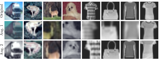
Figure 2: Examples for augmentations used in SidAE showing four CIFAR-10 (left) and four Fashion-MNIST (right) images along with two augmentations.

Input.

SidAE uses two views $\mathbf{x}_{1}$ and $\mathbf{x}_{2}$, which are obtained by applying two augmentations $t_{1}$ and $t_{2}$, which we sample from a set of augmentations $T$. We employ the same augmentation pipeline as in SimSiam (Chen and He,, 2021) for CIFAR-10 which consists of the following transformations stated in PyTorch (Paszke et al.,, 2019) notations: (i) RandomResizedCrop with scale in $[0.2,1]$, (ii) ColorJitter with brightness=0.4, contrast=0.4, saturation=0.4, and hue=0.1 applied with probability $p=0.8$, (iii) RandomGrayscale applied with probability $p=0.2$, and (iv) RandomHorizontalFlip applied with probability $p=0.5$.

For MNIST and Fashion-MNIST, we additionally apply a GaussianBlur with a standard deviation in $[0.1,2.0]$ applied with probability $p=0.5$. This augmentation has usually been included for training Siamese networks on ImageNet. Yet, it has not been used for training SimSiam on CIFAR-10 (Chen and He,, 2021), which we follow to ensure our results are fair and comparable, since CIFAR-10 pictures already have a rather low resolution compared to the complexity of the objects shown. Adding additional blurring would make them hardly identifiable for a human observer, contradicting the reasoning that the transformations should represent factors under which a human would still recognize an object. However, Fashion-MNIST and MNIST samples are still recognizable after blurring. We depict some examples of the transformations in Figure 2.

Figure 3: The components of the models used in our experiments.

Encoder.

The backbone network in the encoder is based on the PyTorch (Paszke et al.,, 2019) implementation of ResNet-18 (He et al.,, 2016). As in SimSiam, we replace the last fully connected layer with a 3-layer projection MLP.

Decoder.

The decoder is another neural network built with the encoder in mind. After the inputs $\mathbf{x}_{1}$ and $\mathbf{x}_{2}$ are encoded into the latent representations $\mathbf{z}_{1}$ and $\mathbf{z}_{2}$, they are fed into the decoder, producing the reconstructions $\mathbf{x}^{\prime}_{1}$ and $\mathbf{x}^{\prime}_{2}$. The decoder mirrors the encoder in that it upsamples the data step-by-step to reconstruct an output of the original input size (three channels of size $32\times 32$). For this purpose, a fully connected layer followed by five transposed convolution layers are stacked on each other. The output channels of each transposed convolution are chosen to mirror the downsampling process of the backbone. Their kernels have a size of $3\times 3$, $\operatorname{padding}=1$, $\operatorname{output\ padding}=1$, and $\operatorname{stride}=2$. While the encoder uses skip connections, we decided against building residual decoders, resulting in a rather simple architecture, decreasing complexity, and keeping it similar to SimSiam.

Predictor.

The predictor is a two-layer MLP, the same as in SimSiam (Chen and He,, 2021). It maps the latent representations $\mathbf{z}_{1}$ and $\mathbf{z}_{2}$ to another latent space to produce two embeddings $\mathbf{p}_{1}$ and $\mathbf{p}_{2}$. Both $\mathbf{z}_{i}$ and $\mathbf{p}_{j}$ ($i,j\in\{1,2\}$ and $i\neq j$) have the same dimensionality since they are compared to each other later. We depict the full structure with the encoder, projector, decoder, and predictor in Figure 3.

Loss.

The loss for SidAE comprises two terms, one for the Siamese and one for the autoencoder part of the network. The former is applied for comparing $\mathbf{z}_{1}$ to $\mathbf{p}_{2}$ and $\mathbf{z}_{2}$ to $\mathbf{p}_{1}$. The latter compares the reconstructions $\mathbf{x}_{1}^{\prime}$ and $\mathbf{x}_{2}^{\prime}$ to the augmented inputs $\mathbf{x}_{1}$ and $\mathbf{x}_{2}$, respectively. In SimSiam, the subcomponents of the loss are scaled by $\frac{1}{2}$, which amounts to scaling the whole loss by $\frac{1}{2}$. We do the same for the autoencoder term of the loss. Additionally, we introduce a weighting term on the Siamese and autoencoder parts of the loss by setting a parameter $w\in[0,1]$. This parameter controls the magnitude of the relative importance of each mechanism in the model. The full loss $L_{\operatorname{sidae}}$ is given by

$$L_{\operatorname{dae}} =\frac{1}{2}D_{\operatorname{mse}}(\mathbf{x},\mathbf{x}^{\prime}_{1})+\frac{1}{2}D_{\operatorname{mse}}(\mathbf{x},\mathbf{x}^{\prime}_{2}),$$

$$L_{\operatorname{si}} =\frac{1}{2}D_{\operatorname{ncs}}(\mathbf{p}_{1},\operatorname{stopgrad}(\mathbf{z}_{2}))+\frac{1}{2}D_{\operatorname{ncs}}(\mathbf{p}_{2},\operatorname{stopgrad}(\mathbf{z}_{1})),$$

$$L_{\operatorname{sidae}} =wL_{\operatorname{dae}}+(1-w)L_{\operatorname{si}},$$

where $L_{\operatorname{dae}}$ is the denoising autoencoder loss and $L_{\operatorname{si}}$ is the Siamese loss. The distance $D_{\operatorname{mse}}$ is a mean squared error (MSE) and $D_{\operatorname{ncs}}$ is the negative cosine similarity (NCS), given by

$$D_{\operatorname{mse}}(\mathbf{a},\mathbf{b})=\frac{1}{d}\sum_{j=1}^{d}(a_{j}-b_{j})^{2}\quad\text{and}\quad D_{\operatorname{ncs}}(\mathbf{a},\mathbf{b})=-\frac{\mathbf{a}^{\mkern-1.5mu\mathsf{T}}\mathbf{b}}{\max(\|\mathbf{a}\|_{2}\cdot\|\mathbf{b}\|_{2},\epsilon)},$$

respectively. Here, $\mathbf{a},\mathbf{b}\in\mathbb{R}^{d}$ and $\epsilon=10^{-8}$ prevents a division by zero.

4 Experiments

We now perform several experiments regarding our proposed SidAE model, compare it against relevant baselines, evaluate the influence of the parameter $w$, and assess how the amount of pre-training impacts a downstream task on several real-world data sets. For clarity and to avoid repetitiveness, we refer below to a denoising autoencoder whenever an autoencoder is mentioned.

4.1 Experimental Setup

Data.

We evaluate on four real-world data sets. CIFAR-10 (Krizhevsky and Hinton,, 2009) consists of 50,000 colored training and 10,000 test images of size $32\times 32$ with three color channels from ten mutually exclusive classes. The MNIST data set (LeCun et al.,, 1995) contains $28\times 28$ pixel images of handwritten digits, thus having ten classes. It consists of 60,000 training and 10,000 test images. Fashion-MNIST (Xiao et al.,, 2017) is similar to MNIST but shows fashion items in ten classes. Finally, STL-10 (Coates et al.,, 2011) also comprises ten classes with a larger resolution of $96\times 96$ pixels with three color channels. It is designed explicitly for self-supervised tasks and has 5,000 labeled training images, 8,000 labeled test images, and additionally 100,000 unlabeled images. We use a downsized version of STL-10 of the same dimensions as CIFAR-10, i.e., $32\times 32$ pixels with three color channels, to keep the models comparable and avoid variability due to different model capacities.

STL-10 is designated for self-supervised or unsupervised pre-training. Thus, we use the unlabeled data for pre-training our models and the train and test sets for training and evaluating the model on the classification task. For the other data sets, we resort to the same training protocol as used in SimSiam (Chen and He,, 2021). We use the training set for self-supervised pre-training and training the classifier on the downstream task. The test set is used for evaluation. In addition, we simulate harder tasks in which we use only a small fraction (i.e., 1%) of the labeled training data for supervised training on the downstream task. The subsets for each data set are drawn randomly but are the same throughout all runs to enable a fair comparison. We always use the full training set (or the unlabeled set in the case of STL-10) for pre-training. To use the same architectures for all data sets, we resize all images to a resolution of $32\times 32$.

Baselines.

We compare SidAE against SimSiam (Chen and He,, 2021) and a denoising autoencoder (Vincent et al.,, 2008). For SimSiam, we use the same architecture as Chen and He, (2021). Thus, the loss of SimSiam is a symmetrized loss of negative cosine similarities between the two views. The encoder of the autoencoder uses a ResNet-18 with a three-layer projection MLP as used in SimSiam and SidAE and the decoder is like in SidAE. The latent dimensionality of SidAE is set to $d_{\text{hid}}=2048$ since it worked best for SimSiam in Chen and He, (2021). We evaluate other choices of latent dimensionalities in the appendix. Since SidAE sees two noisy views at a time, we also provide the autoencoder with two noisy views that are constructed in the same way. We use the mean squared error as a loss for the autoencoder. Furthermore, we consider classification as a downstream task. There, we also compare against a fully supervised ResNet-18.

Setup.

We use Python for all our experiments and implement all models in PyTorch (Paszke et al.,, 2019). All experiments run on a machine with two 32-core AMD Epyc CPUs, 512 GB of RAM, and an NVIDIA A100 GPU with 40GB memory. We re-implement SimSiam based on its original implementation and use the same settings for pre-training. As an optimizer, we use stochastic gradient descent using a cosine decay schedule with an initial learning rate of 0.03, momentum of 0.9, weight decay of 0.0005, and batch size of 512.

We pre-train the backbone networks using SidAE, SimSiam, and a denoising autoencoder for 200 epochs and use the frozen pre-trained backbones as feature extractors for a supervised downstream task, i.e., image classification. Each pre-trained model is evaluated at different stages of pre-training, i.e., after 25, 50, 75, 100, 125, 150, 175, and 200 pre-training epochs, to assess how the duration of pre-training affects the quality of learned representations. We replace the projector MLP within the backbone for the classifier with a fully connected layer with an input dimension equal to $z$. The output dimension is set to match the number of classes in each data set. This downstream task is trained for 50 epochs using a stochastic gradient descent with a learning rate of 0.05, a momentum of 0.9, and a batch size of 256. Since the backbone weights are frozen, only the weights of the last fully connected layer are trained for the downstream task. We later evaluate the scenario of fine-tuning the frozen weights.

4.2 Results

For every experiment, we conduct five runs and report on average accuracies, including standard errors for downstream classification.

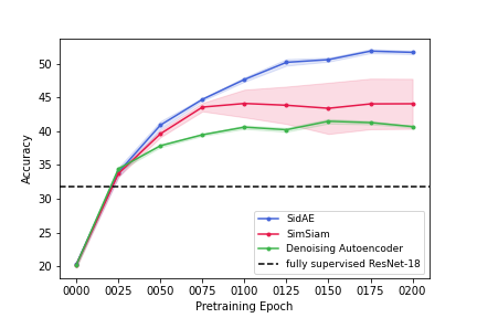
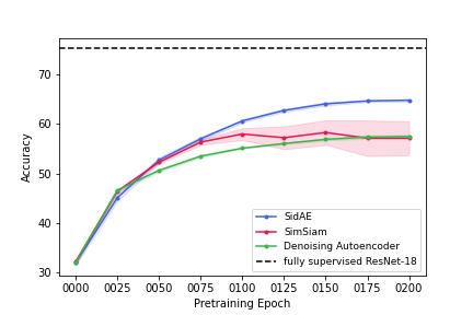
Figure 4: Classification accuracy as downstream task on CIFAR-10 after different pre-training stages using a frozen pre-trained backbone. For downstream training 1% (left) and 100% (right) of training data are used, respectively.

For now, we fix the weight $w\in[0,1]$ interpolating the Siamese and autoencoder loss to $w=0.5$ and evaluate its influence later. Figure 4 shows the effect of pre-training in downstream classification on CIFAR-10. We see that the more pre-training epochs we use, the better the accuracy of the downstream task. The left-hand side depicts the case where we only have 1% of labeled training data for the classification task. There, using only 25 pre-training epochs of the self-supervised methods already outperforms a fully supervised classifier, showing that pre-training helps. Note that when 100% of the labeled training data is available, it does not necessarily outperform a supervised baseline without fine-tuning the encoder, as seen on the right-hand side. Notably, the performance gap for the supervised baseline between 100% and 1% is way higher than for the self-supervised models. These observations support that supervised models need a large amount of training data, performing rather poorly if only little labeled data is available. Note that SimSiam yields the largest standard errors, whereas SidAE is more stable. Overall, SidAE outperforms both the autoencoder and SimSiam.

Table 1: Downstream classification accuracies for SidAE using $w=0.5$, SimSiam, and a denoising Autoencoder averaged over five runs including standard errors.

Data	Pre-Train	SidAE	SimSiam	Autoencoder
CIFAR-10	100%	64.75 (0.27)	57.08 (3.16)	57.44 (0.31)
	1%	51.67 (0.28)	44.06 (3.74)	40.67 (0.25)
Fashion-MNIST	100%	88.78 (0.12)	85.10 (0.09)	87.67 (0.05)
	1%	81.62 (0.22)	77.84 (0.19)	80.20 (0.31)
MNIST	100%	97.80 (0.13)	96.59 (0.60)	97.23 (0.11)
	1%	94.65 (0.49)	79.42 (5.15)	88.41 (0.46)
STL-10	STL-10	61.18 (0.22)	56.74 (0.74)	48.39 (0.22)
	CIFAR-10	66.20 (0.31)	56.64 (0.25)	57.08 (3.16)

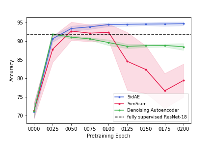
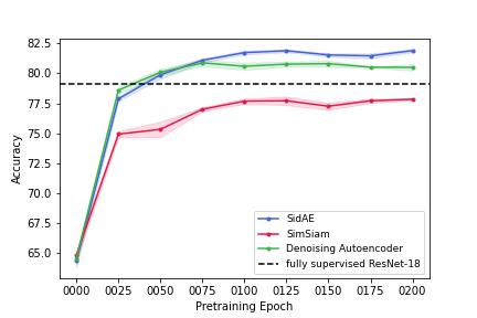
Figure 5: Classification accuracies on MNIST (left) and Fashion-MNIST (right) using 1% of the training data for downstream training.

Table 1 shows classification accuracies averaged over five seeds after 200 pre-training epochs also for the other data sets. There, we can see that SidAE also outperforms its baselines on Fashion-MNIST, MNIST, and STL-10 when compared to its baseline competitors. Figure 5 depicts the classification accuracies on MNIST and Fashion-MNIST using 1% of the training data for downstream training. While for CIFAR-10 (Figure 4), SimSiam either outperformed (1%) or performed on-par (100%) with the autoencoder, the situation is different for MNIST and Fashion-MNIST. SimSiam is especially unstable on MNIST after 100 epochs. On both data sets, the autoencoder is better than SimSiam. Besides, our proposed SidAE model yields better results than the fully supervised baseline.

Figure 6: SidAE: The influence of the weight $w$ on CIFAR-10.

The results for using 100% of the training data for downstream training yield the same outcome and are hence not shown.

The Influence of the weight $w$ in SidAE.

We now investigate the trade-off of the weight $w\in[0,1]$ in the loss. If $w=0$, only the Siamese loss is used, while $w=1$ means that only the autoencoder loss is utilized. Figure 6 depicts the influence of the weight $w$ in SidAE for the 1% case measured again by downstream accuracies. The performance of the classifier when using SidAE with $w\in\{0.125,0.25\}$ is indeed better than the previously used standard choice of $w=0.5$. If the weight for the autoencoder is increased, e.g., using $w\in\{0.75,0.875\}$, the performance decreases and approaches the one from the autoencoder. Note that the best-performing setting of $w=0.125$ increases the performance gap of SidAE in the previous experiment even more. The results are similar for the 100% case and hence not shown. Table 2 (appendix) shows the results for various choices of $w$ on Fashion-MNIST, MNIST, and STL-10.

Figure 7: Classification accuracies on the finetuned downstream task (CIFAR-10) at different pre-training stages using encoders pre-trained with different models using 1% (left) or 100% (right) of the training data for the downstream task.

Finetuning the Downstream Task.

So far, for training the downstream classifier, we have kept the pre-trained weights of the encoder frozen. This was done to judge the capabilities of the pre-training procedure to produce good feature extractors without the encoder being influenced by labeled data. Instead of freezing the weights of the pre-trained encoder, we now finetune them during supervised downstream training. Hence, unlike training a ResNet fully supervised from scratch, the model weights are initialized with those acquired by self-supervised pre-training instead of being initialized randomly. This allows us to investigate whether pre-training boosts performance or whether a model with randomly initialized weights without pre-training can reach the same performance. For this experiment, we set $w=0.125$ within SidAE since it yielded the best performance in the previous experiment (Figure 6).

Figure 7 shows the downstream classification accuracies on CIFAR-10 when we allow for finetuning, i.e., allowing the backbone to adapt to the downstream task. As before, our proposed SidAE model outperforms both self-supervised baselines in almost all cases. In contrast to earlier experiments, all self-supervised models now surpass the supervised baseline for 1% (left side) and for 100% (right side) of the training data. Hence, it is beneficial to use some form of self-supervised pre-training not only in scenarios in which only a small amount of labeled data is available but also if there is a good amount of labeled data.

Results on STL-10.

The STL-10 data is specially designed for self-supervised learning as it comes with a small labeled training set as well as a set of unlabeled training data. We now pre-train the backbone on the unlabeled training data of STL-10 and use the frozen backbone as a feature extractor for the classification downstream task on STL-10 but also on CIFAR-10. This allows us to evaluate whether the feature extraction can be pre-trained on data sets with similar characteristics.

For this experiment, we set $w=0.25$ for SidAE as it yielded the highest downstream accuracy on both data sets. Yet, similar results are obtained for $w=0.125$. The classification accuracies on STL-10 and CIFAR-10 are depicted in Figure 8 on the left- and right-hand side, respectively. For STL-10, we can observe that SidAE and SimSiam both outperform the fully supervised baseline while the denoising autoencoder falls short. The situation differs for CIFAR-10, where the fully supervised baseline is still better. However, note that the performance of SidAE is very similar to the case when the backbone was pre-trained on CIFAR-10 itself (Figure 4). Overall, SidAE performs much better than both self-supervised baselines.

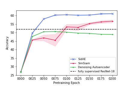
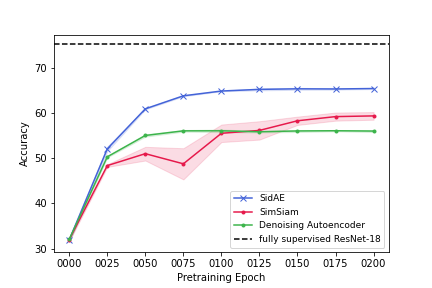
Figure 8: Classification accuracies on STL-10 (left) and CIFAR-10 (right) using an encoder pre-trained with the unlabeled training data of STL-10.

5 Related Work

Many recent state-of-the-art models build on Siamese networks (Caron et al.,, 2020; Chen et al.,, 2020; He et al.,, 2020; Grill et al.,, 2020; Chen and He,, 2021; Liu et al.,, 2022). The idea is to make the model learn that two different versions of one object represent the same object while the factors making them different from each other do not play a role in its identification. The main challenge is to avoid collapsing representations, i.e., where all inputs are assigned to the same feature vector. One widely applied strategy is to use a contrastive loss like InfoNCE (Oord et al.,, 2018; Misra and Maaten,, 2020; Chen et al.,, 2020), where a large amount of negative samples is required for good performance. Various approaches have been presented in this context, such as using large batch sizes (Chen et al.,, 2020), a memory bank to store negatives (Wu et al.,, 2018; Misra and Maaten,, 2020), or a “queue” of negatives retaining negatives from previous batches (He et al.,, 2020). In another approach, Caron et al., (2020) avoid pairwise comparison by mapping embeddings of images to prototype vectors found by online clustering. Those alleviate but do not solve the issues of dealing with negative samples: the computational costs and the quality of the selected samples for training.

Since then, new methods have introduced simpler ways to address the collapsing issue. BYOL (Grill et al.,, 2020) completely circumvents the need for negative samples by applying a momentum encoder, where the weights in one of the branches of the Siamese network are a lagging moving average of the other one. This makes it difficult for the model to converge to a collapsed state but makes the optimization process more complex. SimSiam (Chen and He,, 2021) uses a stop-gradient operation on one of the branches instead, showing that it is sufficient to prevent collapsing solutions. This is not only conceptually straightforward but also results in a simpler implementation. More recently, Liu et al., (2022) show that the stop-gradient operation implicitly introduces a constraint that encourages feature decorrelation, explaining why the simple architecture of SimSiam performs well.

6 Conclusion

This paper is about self-supervised representation learning for which Siamese networks and autoencoders are frequently and successfully used. Siamese networks such as SimSiam (Chen et al.,, 2020) allow for having multiple, possible noisy views on data, and (denoising) autoencoders (Vincent et al.,, 2008) aim to extract essential features of the input in a bottleneck layer by reconstructing a noisy input.

We proposed combining the benefits of Siamese networks and denoising autoencoders for learning meaningful data representations. To achieve this, we introduced a new model called SidAE (Siamese denoising autoencoder). We empirically evaluated the representations learned by our model in various scenarios on several real-world data sets. To do so, we considered a downstream task of classification. Thus, we first pre-trained our model on unlabeled training data in a self-supervised fashion before using the extracted features for learning the supervised classifier. In our experiments, we compared SidAE to SimSiam and a denoising autoencoder.

SidAE consistently outperformed both self-supervised baseline models in terms of mean downstream classification accuracy in all our experiments. Furthermore, compared to SimSiam, SidAE leads to results that are more stable regarding initialization seeds and the amount of used pre-training epochs.

7 Ethics Statement

As with many machine learning models, particularly those based on neural networks, the methods presented here rely on a large amount of data. We see this as the primary source of ethical pitfalls in our work since self-supervised methods can learn from unlabeled data, including poorly curated data. The reason is that the data could implicitly or explicitly contain biases such as over- or underrepresenting certain content. Here, we dealt with classification as an exemplary downstream task. This over- or underrepresentation can potentially lead to undesired performance, for example, in a classification task for underrepresented classes.

Furthermore, using general-purpose feature extractors such as those discussed here should be done cautiously. It is not necessarily clear what exactly the model learns, e.g., what characteristics are extracted from the inputs to base the classification on. We draw attention to cases involving critical decisions and the comprehensibility of those decisions. These issues should also be taken into account in other downstream tasks.

The Influence of the weight $w$ in SidAE.

Within the main body of the paper, we only discussed the influence of $w$ in SidAE for CIFAR-10. Table 2 complements the information from that experiment also with results from Fashion-MNIST, MNIST, and STL-10. The reported accuracies are reported for 200 pre-training epochs and are averaged over five runs, with numbers in parenthesis indicating the standard error. Depending on the data set at hand, the classification accuracies are either stable for various choices of $w$ (e.g., Fashion-MNIST, MNIST 100%) or there is a clear choice of $w$ leading to better results (e.g., CIFAR-10, STL-10).

These experiments show, that lower values of $w$ tend to perform better on CIFAR-10 and STL-10, which are the more challenging data sets. While this pattern does not occur on MNIST and Fashion-MNIST, the performance difference between the worst-performing and best-performing values of $w$ is considerably smaller. This indicates that smaller values of $w$ tend to result in better-performing models.

Table 2: Downstream classification accuracies for different choices of $w$ in SidAE averaged over five runs including standard errors.

Data	Pre-Train	$w=0.125$	$w=0.25$	$w=0.5$	$w=0.75$	$w=0.875$
CIFAR-10	100%	66.20 (0.31)	66.14 (0.18)	64.75 (0.27)	63.07 (0.25)	61.47 (0.23)
	1%	55.61 (0.37)	55.34 (0.29)	51.67 (0.28)	49.21 (0.38)	47.18 (0.41)
Fashion-MNIST	100%	87.31 (0.09)	87.89 (0.09)	88.63 (0.12)	88.78 (0.12)	88.71 (0.10)
	1%	81.49 (0.21)	81.78 (0.27)	81.90 (0.16)	81.62 (0.22)	80.47 (0.29)
MNIST	100%	97.78 (0.04)	97.70 (0.05)	97.80 (0.06)	97.98 (0.08)	98.10 (0.05)
	1%	94.91 (0.20)	94.90 (0.18)	94.65 (0.22)	93.11 (0.13)	92.00 (0.25)
STL-10	STL-10	60.07 (0.18)	61.18 (0.22)	60.44 (0.21)	56.92 (0.20)	53.77 (0.19)
	CIFAR-10	64.12 (0.40)	65.42 (0.16)	65.18 (0.19)	63.33 (0.15)	61.59 (0.20)

Dimensionality of the Latent Space.

According to Chen and He, (2021), SimSiam benefits from a higher dimensional latent space and gets saturated at $d_{\text{hid}}=2048$. Yet, this observation was originally made on ImageNet. We examine if this still holds for CIFAR-10 too, training variants with $d_{\text{hid}}=1024$ and $d_{\text{hid}}=512$. Likewise, we investigate what influence $d_{\text{hid}}$ has on the other self-supervised models. We suspect that a smaller dimensional latent space might be sufficient for this data set since it is of lower dimensionality and less complex than ImageNet. When varying the dimensionality of the latent space, Chen and He, (2021) also adapt the dimensionality of the hidden layer of the predictor MLP such that the hidden layer always has $\frac{1}{4}$ of the size of the feature space. This is done to give the predictor a bottleneck structure. We adopt the same principle here.

The results for SidAE and the denoising autoencoder show a small difference in performance for values of $d_{\text{hid}}$ (within around 1%). Hence, varying the dimensionality of the latent space between 2048, 1024, and 512 does not significantly impact these models. The accuracy may already be saturated at a considerably smaller value of $d_{\text{hid}}$.

SimSiam’s mean accuracy is slightly higher with smaller $d_{\text{hid}}$. A possible interpretation may be that, for higher dimensional latent spaces, additional noise is encoded in the representations, harming downstream performance. Yet, as seen in Figure 9, the standard error of the mean is high, and thus the areas defined by the standard error show considerable overlap.

(a) 1%

(b) 100%

Figure 9: Classification accuracy on the downstream task (CIFAR-10) at different pre-training stages for SimSiam with different dimensionalities of the latent space $d_{\text{hid}}$ using 1% or 100% of the training data for downstream training.

References

- Assran et al., (2023) Assran, M., Duval, Q., Misra, I., Bojanowski, P., Vincent, P., Rabbat, M., LeCun, Y., and Ballas, N. (2023). Self-supervised learning from images with a joint-embedding predictive architecture.
- Baevski et al., (2022) Baevski, A., Hsu, W.-N., Xu, Q., Babu, A., Gu, J., and Auli, M. (2022). Data2vec: A general framework for self-supervised learning in speech, vision and language. In International Conference on Machine Learning, pages 1298–1312. PMLR.
- Caron et al., (2020) Caron, M., Misra, I., Mairal, J., Goyal, P., Bojanowski, P., and Joulin, A. (2020). Unsupervised learning of visual features by contrasting cluster assignments. Advances in Neural Information Processing Systems, 33:9912–9924.
- Chen et al., (2020) Chen, T., Kornblith, S., Norouzi, M., and Hinton, G. (2020). A simple framework for contrastive learning of visual representations. In International conference on machine learning, pages 1597–1607. PMLR.
- Chen and He, (2021) Chen, X. and He, K. (2021). Exploring simple siamese representation learning. In Proceedings of the IEEE/CVF Conference on Computer Vision and Pattern Recognition, pages 15750–15758.
- Coates et al., (2011) Coates, A., Ng, A., and Lee, H. (2011). An analysis of single-layer networks in unsupervised feature learning. In Proceedings of the fourteenth international conference on artificial intelligence and statistics, pages 215–223. JMLR Workshop and Conference Proceedings.
- Doersch et al., (2015) Doersch, C., Gupta, A., and Efros, A. A. (2015). Unsupervised visual representation learning by context prediction. In Proceedings of the IEEE international conference on computer vision, pages 1422–1430.
- Gidaris et al., (2018) Gidaris, S., Singh, P., and Komodakis, N. (2018). Unsupervised representation learning by predicting image rotations. In International Conference on Learning Representations.
- Goodfellow et al., (2014) Goodfellow, I. J., Pouget-Abadie, J., Mirza, M., Xu, B., Warde-Farley, D., Ozair, S., Courville, A., and Bengio, Y. (2014). Generative adversarial nets. In Proceedings of the 27th International Conference on Neural Information Processing Systems-Volume 2, pages 2672–2680.
- Grill et al., (2020) Grill, J.-B., Strub, F., Altché, F., Tallec, C., Richemond, P., Buchatskaya, E., Doersch, C., Avila Pires, B., Guo, Z., Gheshlaghi Azar, M., et al. (2020). Bootstrap your own latent-a new approach to self-supervised learning. Advances in neural information processing systems, 33:21271–21284.
- He et al., (2020) He, K., Fan, H., Wu, Y., Xie, S., and Girshick, R. (2020). Momentum contrast for unsupervised visual representation learning. In Proceedings of the IEEE/CVF conference on computer vision and pattern recognition, pages 9729–9738.
- He et al., (2016) He, K., Zhang, X., Ren, S., and Sun, J. (2016). Deep residual learning for image recognition. In Proceedings of the IEEE conference on computer vision and pattern recognition, pages 770–778.
- Henaff, (2020) Henaff, O. (2020). Data-efficient image recognition with contrastive predictive coding. In Proceedings of the 37th International Conference on Machine Learning, pages 4182–4192. PMLR.
- Hinton and Salakhutdinov, (2006) Hinton, G. E. and Salakhutdinov, R. R. (2006). Reducing the dimensionality of data with neural networks. science, 313(5786):504–507.
- Jing and Tian, (2020) Jing, L. and Tian, Y. (2020). Self-supervised visual feature learning with deep neural networks: A survey. IEEE transactions on pattern analysis and machine intelligence, 43(11):4037–4058.
- Krizhevsky and Hinton, (2009) Krizhevsky, A. and Hinton, G. (2009). Learning multiple layers of features from tiny images. Technical report.
- LeCun et al., (1995) LeCun, Y., Jackel, L. D., Bottou, L., Cortes, C., Denker, J. S., Drucker, H., Guyon, I., Muller, U. A., Sackinger, E., Simard, P., et al. (1995). Learning algorithms for classification: A comparison on handwritten digit recognition. Neural networks: the statistical mechanics perspective, 261(276):2.
- Li et al., (2017) Li, Y., Fang, C., Yang, J., Wang, Z., Lu, X., and Yang, M.-H. (2017). Universal style transfer via feature transforms. Advances in neural information processing systems, 30.
- Linsker, (1989) Linsker, R. (1989). How to generate ordered maps by maximizing the mutual information between input and output signals. Neural computation, 1(3):402–411.
- Liu et al., (2022) Liu, K.-J., Suganuma, M., and Okatani, T. (2022). Bridging the gap from asymmetry tricks to decorrelation principles in non-contrastive self-supervised learning. Advances in Neural Information Processing Systems, 35:19824–19835.
- Misra and Maaten, (2020) Misra, I. and Maaten, L. v. d. (2020). Self-supervised learning of pretext-invariant representations. In Proceedings of the IEEE/CVF Conference on Computer Vision and Pattern Recognition, pages 6707–6717.
- Noroozi and Favaro, (2016) Noroozi, M. and Favaro, P. (2016). Unsupervised learning of visual representations by solving jigsaw puzzles. In European conference on computer vision, pages 69–84. Springer.
- Oord et al., (2018) Oord, A. v. d., Li, Y., and Vinyals, O. (2018). Representation learning with contrastive predictive coding. arXiv preprint arXiv:1807.03748.
- Paszke et al., (2019) Paszke, A., Gross, S., Massa, F., Lerer, A., Bradbury, J., Chanan, G., Killeen, T., Lin, Z., Gimelshein, N., Antiga, L., et al. (2019). Pytorch: An imperative style, high-performance deep learning library. Advances in neural information processing systems, 32.
- Pathak et al., (2016) Pathak, D., Krahenbuhl, P., Donahue, J., Darrell, T., and Efros, A. A. (2016). Context encoders: Feature learning by inpainting. In Proceedings of the IEEE conference on computer vision and pattern recognition, pages 2536–2544.
- Tian et al., (2020) Tian, Y., Sun, C., Poole, B., Krishnan, D., Schmid, C., and Isola, P. (2020). What makes for good views for contrastive learning? Advances in Neural Information Processing Systems, 33:6827–6839.
- Vincent et al., (2008) Vincent, P., Larochelle, H., Bengio, Y., and Manzagol, P.-A. (2008). Extracting and composing robust features with denoising autoencoders. In Proceedings of the 25th international conference on Machine learning, pages 1096–1103.
- Vincent et al., (2010) Vincent, P., Larochelle, H., Lajoie, I., Bengio, Y., Manzagol, P.-A., and Bottou, L. (2010). Stacked denoising autoencoders: Learning useful representations in a deep network with a local denoising criterion. Journal of machine learning research, 11(12).
- Wickramasinghe et al., (2021) Wickramasinghe, C. S., Marino, D. L., and Manic, M. (2021). Resnet autoencoders for unsupervised feature learning from high-dimensional data: Deep models resistant to performance degradation. IEEE Access, 9:40511–40520.
- Wu et al., (2018) Wu, Z., Xiong, Y., Yu, S. X., and Lin, D. (2018). Unsupervised feature learning via non-parametric instance discrimination. In Proceedings of the IEEE conference on computer vision and pattern recognition, pages 3733–3742.
- Xiao et al., (2017) Xiao, H., Rasul, K., and Vollgraf, R. (2017). Fashion-mnist: a novel image dataset for benchmarking machine learning algorithms.
- Zhang et al., (2016) Zhang, R., Isola, P., and Efros, A. A. (2016). Colorful image colorization. In European conference on computer vision, pages 649–666. Springer.