PWESuite: Phonetic Word Embeddings and Tasks They Facilitate

Abstract

Word embeddings that map words into a fixed-dimensional vector space are the backbone of modern NLP. Most word embedding methods encode semantic information. However, phonetic information, which is important for some tasks, is often overlooked. In this work, we develop several novel methods which leverage articulatory features to build phonetically informed word embeddings, and present a set of phonetic word embeddings to encourage their community development, evaluation and use. While several methods for learning phonetic word embeddings already exist, there is a lack of consistency in evaluating their effectiveness. Thus, we also proposes several ways to evaluate both intrinsic aspects of phonetic word embeddings, such as word retrieval and correlation with sound similarity, and extrinsic performances, such as rhyme and cognate detection and sound analogies. We hope that our suite of tasks will promote reproducibility and provide direction for future research on phonetic word embeddings.

equ[Equation][List of equations]

PWESuite: Phonetic Word Embeddings and Tasks They Facilitate

  Vilém Zouhar${}^{\text{ {{\color[rgb]{0,0.1,0.4}{E}}}}}$          Kalvin Chang${}^{\text{ {{\color[rgb]{0.5,0.1,0.1}{C}}}}}$        Chenxuan Cui${}^{\text{ {{\color[rgb]{0.5,0.1,0.1}{C}}}}}$       Nathaniel Carlson${}^{\text{ {{\color[rgb]{0,0.1,0.2}{Y}}}}}$ Nathaniel Robinson${}^{\text{ {{\color[rgb]{0.5,0.1,0.1}{C}}}}}$     Mrinmaya Sachan${}^{\text{ {{\color[rgb]{0,0.1,0.4}{E}}}}}$    David Mortensen${}^{\text{ {{\color[rgb]{0.5,0.1,0.1}{C}}}}}$ ${}^{\text{ {{\color[rgb]{0,0.1,0.4}{E}}}}}$Department of Computer Science, ETH Zurich ${}^{\text{ {{\color[rgb]{0.5,0.1,0.1}{C}}}}}$Language Technologies Institute, Carnegie Mellon University ${}^{\text{ {{\color[rgb]{0,0.1,0.2}{Y}}}}}$Department of Computer Science, Brigham Young University {vzouhar,msachan}@ethz.ch  natbcar@gmail.com {kalvinc,cxcui,nrrobins,dmortens}@cs.cmu.edu

Code: github.com/zouharvi/pwesuite

Dataset: huggingface.co/datasets/ zouharvi/pwesuite-eval

1 Introduction

Word embeddings are an omnipresent tool in modern NLP (Le and Mikolov, 2014; Pennington et al., 2014; Almeida and Xexéo, 2019, inter alia). Their main benefit lies in compressing information useful to the user into vectors with fixed numbers of dimensions. These vectors can be easily used as features for machine learning applications and their study can reveal insights into language and its use. Word embeddings are often trained using methods of distributional semantics (Camacho-Collados and Pilehvar, 2018) and hence bear semantic information.

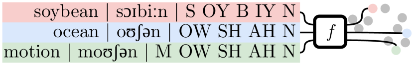
Figure 1: Embedding function $f$ which projects words in various forms (left) to a vector space (right).

In these cases, for example, the embedding for the word carrot encodes in some way that it is more like embeddings for other vegetables than the embedding for ocean. Nevertheless, some applications may require a different type of information to be encoded. For a poem generation model, for instance, the embedding of a word might reflect that ocean rhymes with motion and not with a soybean, even though the characters at the ends of the words would suggest otherwise. Such embeddings, which contain phonetic information, are referred to as phonetic word embeddings, were studied in recent years (Bengio and Heigold, 2014; Parrish, 2017; El-Geish, 2019; Yang and Hirschberg, 2019; Hu et al., 2020; Sharma et al., 2021). The basic premise is that words with similar pronunciations are projected to vectors that are near each other in the embedding space.

In this work, we introduce multiple methods for creating phonetic word embeddings. They range from intuitive baselines to more complex techniques using metric and contrastive learning. More importantly, however, we include an evaluation suite for testing the performance of phonetic embeddings. The motivations for this are two-fold. First, prior works are inconsistent in evaluating their models. This prevents the field from observing long-term improvements of such embeddings and from making fair comparisons across different approaches. Secondly, when a practitioner is deciding which phonetic word embedding method to use, the go-to approach is to first apply the embeddings (generally fast) and then train a downstream model on those embeddings (compute and time intensive). Instead, intrinsic embedding evaluation metrics (cheap)—if shown to correlate well with extrinsic metrics—could provide useful signals in embedding method selection prior to training of downstream models (expensive). In contrast to semantic word embeddings (Bakarov, 2018), we show that intrinsic and extrinsic metrics for phonetic word embeddings generally correlate with each other. While some work on evaluating acoustic word embeddings exists (Ghannay et al., 2016), this work specializes in phonetic word embeddings for text, not speech.

Our contributions are threefold:

• a survey of existing phonetic embeddings,

• four novel methods for phonetic word embedding, ranging from simple baselines to complex models, and

• an evaluation suite for such embeddings.

2 Survey of Phonetic Embeddings

Formally, given some alphabet $\Sigma$ and a dataset of words $\mathcal{W}\subseteq\Sigma^{*}$, $d$-dimensional word embeddings are a function $f:\mathcal{W}\rightarrow\mathbb{R}^{d}$ where $\Sigma$ is some alphabet. In words, they take an element from the set $\Sigma^{*}$ (set of all possible words over the alphabet $\Sigma$) and produce a $d$-dimensional vector of numbers. Note that for most embedding functions, $\mathcal{W}$ is a finite set of words and the embeddings are not defined for unseen words (Mikolov et al., 2013a; Pennington et al., 2014). In contrast, other embedding functions—which we dub open—are able to provide an embedding for any word $x\in\Sigma^{*}$ (Bojanowski et al., 2017). An illustration of a phonetic word embedding function is shown in Figure 1. We will work with 3 different alphabets: characters $\Sigma_{C}$, IPA symbols $\Sigma_{P}$ and ARPAbet symbols $\Sigma_{A}$. When the specific alphabet choice is not important, we use $\Sigma$. We review some of the semantic embeddings that satisfy this in Section 5 and now focus on prior work on phonetic word embeddings.

2.1 Poetic Sound Similarity

Parrish (2017) learns word embeddings capturing pronunciation similarity for poetry generation for words in the CMU Pronouncing Dictionary Carnegie Mellon Speech Group (2014). First, each phoneme is mapped to a set of phonetic features $\mathcal{F}$ using the function $\textsc{P2F}:\Sigma_{A}\rightarrow 2^{\mathcal{F}}$. From this sequence of sets, bi-grams of phonetic features are created (using cross-product $\times$ between sets $a_{i}$ and $a_{i+1}$) and counted. The function CountVec simply counts the number of occurrences of a specific feature and puts them in a vector of a constant dimension. The resulting vector is then reduced using PCA (F.R.S., 1901) to the target word embedding dimension $d$.

$$\textsc{W2F}(x) =\langle\textsc{P2F}(x_{i})|x_{i}\in x\rangle\qquad\quad\text{{\color[rgb]{.5,.5,.5}(array)}}$$ (1)

$$\textsc{F2V}(a) =\textsc{CountVec.}\big{(}\bigcup_{1\leq i\leq|a|-1}a_{i}\times a_{i+1}\big{)}$$ (2)

$$f_{\textsc{PAR}} =\textsc{PCA}_{d}(\{\textsc{F2V}(\textsc{W2F}(x))|x\in\mathcal{W}\})$$ (3)

Note that the function $f_{\textsc{PAR}}$ can provide embeddings even for words unseen during training. This is because the only component dependent on the training data is the PCA over the vector of bigram counts, which can also be applied to new vectors.

2.2 phoneme2vec

Fang et al. (2020) do not use hand-crafted feature functions but rather learn phoneme embeddings using a more complex, deep-learning, model. They start with a gold sequence of phonemes $(x_{i})$ and a hypothesis sequence of phonemes $(y_{i})$ which is the output of an automatic speech recognition (ASR) system. The gold sequence (from the ASR perspective) is first consumed by an LSTM model, yielding the initial hidden state $h_{0}$. From this hidden state, the phonemes $(y_{i})$ are decoded using teacher forcing. This means that upon predicting $\hat{y_{i}}$, the model receives the correct $y_{i}$ as the input. The phoneme embedding matrix $V$ is trained jointly with the model weights and later constitutes the embedding function.

$$h_{0}=\textsc{LSTM}(\langle x_{i}\cdot V|x_{i}\in x\rangle)$$ (4)

$$\mathcal{L}_{\text{p2v}}=\sum_{0<i\leq|y|}-\log\big{(}\operatorname*{softmax}(\hskip 51.21495pt$$ (5)

$$\hskip 85.35826pt\textsc{LSTM}(y_{i-1}\cdot V|y_{<i-1}))_{y_{i}}\big{)}$$

Note that these embeddings are phoneme-level and not word-level and hence a direct comparison is not possible. To obtain word-level embeddings from their phoneme embeddings, we use mean pooling across dimensions for each word. Further, in contrast to other embeddings, these phoneme embeddings are only 50-dimensional, putting them at a greater disadvantage because they have less space to store the relevant information. We revisit the question of dimensionality in Section 5.5.

2.3 Phonetic Similarity Embeddings

Sharma et al. (2021) propose a novel vowel-weighted phonetic similarity metric to compute similarities between words. They then use it for training phonetic word embeddings which should share some properties with this similarity function. This is in contrast to the previous approaches, where the embedding training was done indirectly on some auxiliary task. Given a sound similarity function $S_{\text{PSE}}$, they construct a matrix of similarity scores $S\in\mathbb{R}^{|\mathcal{W}|\times|\mathcal{W}|}$ such that $S_{i,j}=S_{\text{PSE}}(\mathcal{W}_{i},\mathcal{W}_{j})$. On this matrix, they use non-negative matrix factorization to learn the embedding matrix $V\in\mathbb{R}^{|\mathcal{W}|\times d}$ such that the following loss is minimized

$$\mathcal{L}_{\text{PSE}}=||S-V\cdot V^{T}||^{2}$$ (6)

Then, the $i$-th row of $V$ contains the embedding for $i$-th word from $\mathcal{W}$. A major disadvantage of this approach is that it cannot be used for embedding new words because the matrix $V$ would need to be recomputed again. Although their sound similarity function $S_{\text{PSE}}$ is available only for English, we use it also for other languages, admittedly making the comparison unfair.

3 Our Models

In this section, we first introduce several baselines. We then describe PanPhon’s articulatory distance and explain models trained with supervision from this function. See Appendix A for the hyperparameters of presented models and Appendix B for the negative result of phonemic language modeling.

3.1 Count-based Vectors

Perhaps the most straightforward way of creating a vector representation for a sequence of input characters or phonemes $x\in\Sigma^{*}$ is simply counting n-grams in this sequence. We use a TF-IDF vectorizer of 1-,2- and 3-grams (using cross-product $\times$) with a maximum of 300 features, which then become our embeddings.

$$\textsc{C2V}(x) =\bigcup_{\begin{subarray}{c}n\in\{1,2,3\}\\ 1\leq i\leq|x|-n+1\end{subarray}}x_{i}\times\ldots\times x_{i+n-1}$$ (7)

$$f_{\text{count}}(x) =\textsc{TF-IDF}_{\text{feat.}=d}(\{\textsc{C2F}(x)|x\in\mathcal{W}\})$$ (8)

Although there are multiple ways to set up this pipeline, such as including PCA or normalization, we do no post-processing for simplicity.

3.2 Autoencoder

Another common approach, though less interpretable, for vector representation with fixed dimension size is an encoder-decoder autoencoder. Specifically, we use this architecture together with forced-teacher decoding and use the bottleneck vector as the phonetic word embedding.

$$f_{\theta}(x)=\textsc{LSTM}(x|\theta)\,\qquad\qquad{\color[rgb]{.5,.5,.5}\text{(encoder)}}$$ (9)

$$d_{\theta^{\prime}}(x)=\textsc{LSTM}(x|\theta^{\prime})\qquad\qquad{\color[rgb]{.5,.5,.5}\text{(decoder)}}$$ (10)

$$\mathcal{L}_{\text{auto.}}=\sum_{0<i\leq|x|}-\log\text{softmax}(d_{\theta^{\prime}}(f_{\theta}(x)|x_{<i})_{x_{i}})$$ (11)

Recall that we can represent words in different ways, such as characters or IPA symbols.

3.3 Phonetic Embeddings With PanPhon

3.3.1 Articulatory Features and Distance

We first bring to attention the articulatory feature vectors by Mortensen et al. (2016). Each phoneme segment is mapped to a vector which marks 24 different features, such as whether the phoneme segment is produced with a nasal airflow or if the segment is produced with the tongue body raised or lowered. We denote $a:\Sigma_{P}\rightarrow\{-1,0,+1\}^{24}$ as the function which maps a phoneme segment into a vector of articulatory features.

The articulatory distance, also called feature edit distance (Mortensen et al., 2016), is a version of Levenshtein distance with custom operation costs. Specifically, the substitution cost is proportional to the Hamming distance between the source and target when they are represented as articulatory feature vectors. It can be defined in a recursive dynamic-programming manner:

$$A_{i,j}(x,x^{\prime}) =\min\left\{\begin{array}[]{l}A_{i-1,j}(x,x^{\prime})+d(x)\\ A_{i,j-1}(x,x^{\prime})+i(x^{\prime})\\ A_{i-1,j-1}(x,x^{\prime})+s(x_{i},x^{\prime}_{j})\\ \end{array}\right.$$ (16)

$$A(x,x^{\prime}) =A_{|x|,|x^{\prime}|}(x,x^{\prime})$$ (17)

where $d$ and $i$ are deletion and insertion costs, which we set to constant $1$. The function $s$ is a substitution cost, defined as the number of elements (normalized) that need to be changed to render the two articulatory vectors identical:

$$s(x,x^{\prime})=\frac{1}{24}\sum_{i=1}^{24}|a(x)_{i}-a(x^{\prime})_{i}|$$ (18)

The articulatory distance $A$ induces a metric space-like structure on top of words in $\Sigma^{*}$. Furthermore, it quantifies the phonetic similarity between a pair of words, capturing the intuition that /pæt/ and /bæt/ are phonetically closer than /pæt/ and /hæt/, for example.

3.3.2 Metric Learning

Our requirements for the embedding model $f$ are that it takes the word in some form as an input and produces a vector of fixed dimension as an output. To this end, we use an LSTM-based model and extract the last hidden state for the embeddings. We use both characters $\Sigma_{C}$, IPA symbols $\Sigma_{P}$ (Section 2) and articulatory feature vectors as the input word representation. We discuss these choices and especially their effect on performance and transferability in Section 5.3.

We now have a function $f$ that produces a vector for each input word. However, it is not trained to produce vectors that satisfy our requirements for phonetic embeddings. We, therefore, define the following differentiable loss where $A$ is the articulatory distance from PanPhon.

$$\mathcal{L}_{\text{dist.}}=\frac{1}{|\mathcal{W}|}\sum_{\begin{subarray}{c}x_{a}\in\mathcal{W}\\ x_{b}\sim\mathcal{W}\end{subarray}}\Big{(}\,||f_{\theta}(x_{a})-f_{\theta}(x_{b})||^{2}\hskip 36.98857pt$$

$$\hskip 119.50157pt-A(x_{a},x_{b})\Big{)}^{2}$$ (19)

This forces the embeddings to be spaced in the same way as the articulatory distance ($A$, Section 3.3.1) would space them. We note that metric learning (learning a function to space output vectors similarly to some other metric) is not novel (Yang and Jin, 2006; Kulis et al., 2013; Bellet et al., 2015; Kaya and Bilge, 2019) and was used to train embeddings by Yang and Hirschberg (2019).

3.3.3 Triplet Margin loss

While the previous approach forces the embeddings to be spaced exactly as by the articulatory distance function $A$, we may relax the constraint so only the structure (ordering) is preserved. This leads to the triplet margin loss:

$$\mathcal{L}_{\text{triplet}}=\max\begin{cases}0\\ \alpha+|f_{\theta}(x_{a})-f_{\theta}(x_{p})|\\ \quad-|f_{\theta}(x_{a})-f_{\theta}(x_{n})|\end{cases}$$ (20)

We consider all possible ordered triplets of distinct words $(x_{a},x_{p},x_{n})$ such that $A(x_{a},x_{p})<A(x_{a},x_{n})$. We refer to $x_{a}$ as the anchor, $x_{p}$ as the positive example, and $x_{n}$ as the negative example. We then minimize $\mathcal{L}_{\text{triplet}}$ over all valid triplets. This allows us to learn $\theta$ for an embedding function $f_{\theta}$ that preserves the local neighbourhoods of words defined by $A(x,x^{\prime})$. In addition, we modify the function $f_{\theta}$ by applying attention to all hidden states extracted from the last layer of the LSTM encoder. This allows our model to focus on phonemes that are potentially more useful when trying to summarize the phonetic information in a word. This approach was also used by Yang and Hirschberg (2019) to learn acoustic word embeddings. Oh et al. (2022) found success leveraging layer attentive pooling and contrastive learning to extract embeddings from pre-trained language models.

4 Evaluation Suite

In this section, we introduce in detail all the embedding evaluation metrics that we use in our suite. We draw inspiration from evaluating semantic word embeddings (Bakarov, 2018) and prior work on phonetic word embeddings (Parrish, 2017). In some cases, the distinction between intrinsic and extrinsic evaluations is unclear (e.g., retrieval and analogies). However, the main characteristic of intrinsic evaluation is that they are fast to compute and are not part of any specific application. In contrast, extrinsic evaluation metrics directly measure the usefulness of the embeddings for a particular NLP application.

We use 9 phonologically diverse languages: Amharic,^∗ Bengali,^∗ English, French, German, Polish, Spanish, Swahili, and Uzbek. The non-English data (200k tokens for each language) is sourced from CC-100 (Wenzek et al., 2020; Conneau et al., 2020), while the English data (125k tokens) comes from the CMU Pronouncing Dictionary (Carnegie Mellon Speech Group, 2014). The set of languages can be extended in future versions of the evaluation suite.

4.1 Intrinsic Evaluation

4.1.1 Articulatory Distance

While probing for semantic information in words is already established (Miaschi and Dell’Orletta, 2020), it is not clear what information phonetic word embeddings should contain. However, one common desideratum is that they should capture the concept of sound similarity. Recall from Section 2 that phonetic word embeddings are a function $f:\Sigma^{*}\rightarrow\mathbb{R}^{d}$. In the vector space of $\mathbb{R}^{d}$, there are two widely used notions of similarity $S$. The first is the negative $L_{2}$ distance and the other is the cosine distance. Consider three words $x,x^{\prime}$ and $x^{\prime\prime}$. By using one of these on the top of the embeddings from $f$ as $S(f(x),f(x^{\prime}))$, we obtain a measure of similarity between the two embeddings. On the other hand, since we have prior notions of similarity $S_{P}$ between the words, e.g., based on a rule-based function, we can use this to represent the similarity between the words: $S_{P}(x,x^{\prime})$. We want to have embeddings $f$ such that $f\circ S$ produces results close to $S_{P}$. There are at least two ways to verify that the similarity results are close. In the first one, we care about the exact values. For example, if $S_{P}(x,x^{\prime})=0.5,S_{P}(x,x^{\prime\prime})=0.1$, we want $S(f(x),f(x^{\prime}))=0.5,S(f(x),f(x^{\prime\prime}))=0.1$. We can measure this using Pearson’s correlation coefficient between $f\circ S$ and $S_{P}$. On the other hand, we may not always care about the specific similarity numbers. Following the previous example, we would only care that $S(f(x),f(x^{\prime}))>S(f(x),f(x^{\prime}))$. This is measured using the Spearman’s correlation coefficient between $f\circ S$ and $S_{P}$. For the rule-based similarity metric $S_{P}$, we use articulatory distance from PanPhon (Mortensen et al., 2016), as described in Section 3.3.1.

		intrinsic			extrinsic			overall
	Model	Human Sim.	Art. Dist.	Retrieval	Analogies	Rhyme	Cognate
		(Pearson)	(Pearson)	(rank perc.)	(Acc@1)	(accuracy)	(accuracy)
Ours	Metric Learner	0.46	0.94	0.98	84%	83%	64%	0.78
	Triplet Margin	0.65	0.96	1.00	100%	77%	66%	0.84 $\star$
	Count-based	0.82	0.10	0.84	13%	79%	68%	0.56
	Autoencoder	0.49	0.16	0.73	50%	61%	50%	0.50
Others’	Poetic Sound Sim.	0.74	0.12	0.78	35%	60%	57%	0.53
	phoneme2vec	0.77	0.09	0.80	17%	88%	64%	0.56
	Phon. Sim. Embd.	0.16	0.05	0.50	0%	51%	52%	0.29
Semantic	BPEmb	0.23	0.08	0.60	5%	54%	66%	0.36
	fastText	0.25	0.12	0.64	2%	58%	68%	0.38
	BERT	0.10	0.34	0.69	4%	58%	63%	0.40
	INSTRUCTOR	0.60	0.12	0.73	7%	54%	66%	0.45

Table 1: Embedding method performance in our evaluation suite. Higher number is always better.

4.1.2 Human Judgement

Vitz and Winkler (1973) performed an experiment where they asked people to judge the sound similarity of English words. For selected word pairs, we denote the collected judgements (number from 0–least similar to 1–identical) using the function $S_{H}$. For example, $S_{H}(\textit{slant},\textit{plant)}=0.9$ and $S_{H}(\textit{plots},\textit{plant})=0.4$. Similarly to the previous task, we compute the correlations between $f\circ S$ and $S_{H}$. The reasons this is not a replacement for the articulatory distance task are the small corpus size and its limitation to English. In perspective, the Pearson correlation of $A$ and $S_{H}$ is $-0.74$.

4.1.3 Retrieval

An important usage of word embeddings is the retrieval of associated words, which is also later utilized in the analogies extrinsic evaluation and other applications. Success in this task means that the new embedding space has the same local neighbourhood as the original space induced by some non-vector-based metric. Given a dataset of words $\mathcal{W}$ and one specific word $w\in\mathcal{W}$, we sort $\mathcal{W}\setminus\{w\}$ based on both $f\circ S$ and $S_{P}$. Based on this ordering, we define the immediate neighbour of $w$ based on $S_{P}$, denoted $w_{N}$ and ask the question What is the average rank of $w_{N}$ in the ordering by $f\circ S$? If the similarity given by $f\circ S$ is copying $S_{P}$ perfectly, then the rank will be 0 because $w_{N}$ will be the closest to $w$ in $f\circ S$.

Again, for $S_{P}$ we use the articulatory distance $A$ (Section 3.3.1). Even though there are a variety of possible metrics to measure success in retrieval, we focus on the average rank. We further cap the retrieval neighbourhood to $n=1000$ samples and compute percentile rank as $\frac{n-r}{n}$. This choice is motivated by the metric being bounded between 0 (worst) and 1 (best), which will become important for overall evaluation later (Section 4.3).

See a brief error analysis of one model for this task in Appendix D.

4.2 Extrinsic Evaluation

4.2.1 Rhyme Detection

There are multiple types of word rhymes, most of which are based around two words sounding similarly. We focus on perfect rhymes: when the sounds from the last stressed syllables are identical. An example is grown and loan, even though the surface character form does not suggest it. Clearly, this task can be deterministically solved by having access to the articulatory and stress information of the concerned words. Nevertheless, we wish to see whether this information can be encoded in a fixed-length vector produced by $f$. We create a balanced binary prediction task for rhyme detection in English and train a small multi-layer perceptron classifier (see Appendix A) on top of pairs of word embeddings. The linking hypothesis is that the higher the accuracy, the more useful information for the task there is in the embeddings.

4.2.2 Cognate Detection

Cognates are words in different languages that share a common origin. Similarly to rhyme detection, we frame cognate detection as a binary classification task where the input is a potential cognate pair. CogNet Batsuren et al. (2019) is a large cognate dataset that contains many languages, making it ideal to evaluate the usefulness of phonetic embeddings. We add non-cognate, distractor pairs in the dataset by finding the orthographically closest word that is not a known cognate. For example, plant${}_{\text{EN}}$ and plante${}_{\text{FR}}$ are cognates, while plant${}_{\text{EN}}$ and plane${}_{\text{EN}}$ are not. Although cognates also preserve some of the similarities in the meaning, we detect them using phonetic characteristics.

4.2.3 Sound Analogies

Just as distributional semantic vectors can complete word-level analogies such as man:woman $\leftrightarrow$ king:queen (Mikolov et al., 2013b), so too should well-trained phonetic word embeddings capture sound analogies. For example of a sound analogy, consider /dIn/ : /tIn/ $\leftrightarrow$ /zIn/ : /sIn/. The difference within the pairs is [$\pm$voice] in the first phoneme segment of each word.

With this intuition in mind, we define a perturbation as a pair of phonemes $(p,q)$ whose articulatory distance is $s(p,q)=1$ (see Equation 18 in Section 3.3.1). We then create a sound analogy corpus of 200 quadruplets $w_{1}:w_{2}\leftrightarrow w_{3}:w_{4}$ for each language, with the following procedures:

1. Choose a random word $w_{1}\in\mathcal{W}$ and one of its phonemes on random position $i$: $p_{1}=w_{1,i}$.

2. Randomly select two perturbations of the same phonetic feature so that $p_{1}:p_{2}\leftrightarrow p_{3}:p_{4}$, for example /t/ : /d/ $\leftrightarrow$ /s/ : /z/.

3. Create $w_{2}$, $w_{3}$, and $w_{4}$ by duplicating $w_{1}$ and replacing $w_{1,i}$ with $p_{2}$, $p_{3}$, and $p_{4}$.

We apply the above procedure 1 or 2 times to create 200 analogous quadruplets with 1 or 2 perturbations (evenly split). We then measure the Acc@1 to retrieve $w_{4}$ from $\mathcal{W}\cup\{w_{4}\}$. This means that we simply measure how many times the closest neighbour of $w_{2}-w_{1}+w_{3}$ is $w_{4}$. Our analogy task is different from that of Parrish (2017) who focused on derivational changes.

4.3 Overall Score

Since all the measured metrics are bounded between 0 and 1, we can define the overall score for our evaluation suite as the arithmetic average of results from each task. We mainly consider the results of all available languages averaged but later in Section 5.3 discuss results per language as well. To allow for future extensions in terms of languages and tasks, this evaluation suite is versioned, with the version described in this paper being v1.0.

5 Evaluation

In this section, we compare all the aforementioned embedding models using our evaluation suite. We show the results in Table 1 with three categories of models. Our models trained using some PanPhon supervision or features (Section 3) are given first, followed by other phonetic word embedding models (Section 2). We also include non-phonetic word embeddings, not as a fair baseline for comparison but to show that these embeddings are different from phonetic word embeddings and are not suited for our tasks: fastText (Grave et al., 2018), BPEmb (Heinzerling and Strube, 2018), BERT (Devlin et al., 2019) and INSTRUCTOR (Su et al., 2022). We chose these embeddings because they are open (i.e., they provide embeddings even to words unseen in the training data). All of these embeddings except for BERT and INSTRUCTOR are 300-dimensional. We discuss the relationship between embedding dimensionality and task performance in more detail in Section 5.5.

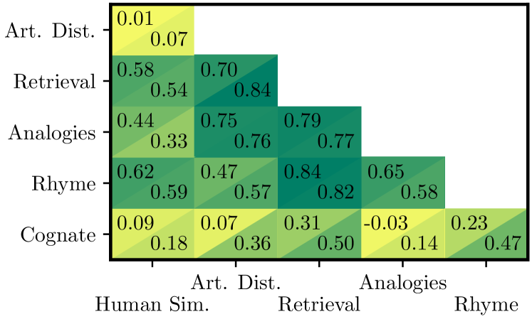
Figure 2: Spearman (upper left) and Pearson (lower right) correlations between embedding performances on suite tasks. All embeddings from Table 1 are used.

5.1 Model Comparison

In Table 1 we show the performance of all previously described models. The Triplet Margin model is better than Metric Learner, despite the fact that it receives less direct supervision during training. However, it also requires the longest time to train (Appendix A). Despite the fact that it is better than all other models and also the more naive approaches, the best model for human similarity is a very simple Count-based model. Unsurprisingly, semantic word embeddings perform worse than explicit phonetic embeddings, most notably on human similarity and analogies.

We now examine how much the performance on one task (particularly an intrinsic one) is predictive of performance on another task. We measure this across all systems in Table 1 and revisit this topic later for creating variations of the same model. For lexical/semantic word embeddings, Bakarov (2018) notes that the individual tasks do not correlate among each other. However, in Figure 2, we find the contrary for some of the selected tasks (e.g., Retrieval and Rhyme or Retrieval and Analogies). Importantly, there is no strong negative correlation between any tasks, suggesting that performance on one task is not a tradeoff with another.

Model	Art.	IPA	Text
Metric Learner	0.78	0.64	0.62
Triplet Margin	0.84	0.84	0.79
Autoencoder	0.50	0.41	0.41
Count-based	-	0.56	0.51

Table 2: Overall performance of models with various input features. Art. = PanPhon articulatory features.

5.2 Input Features

For all of our models, it is possible to choose the input feature type, which has an impact on the performance, as shown in Table 2. Unsurprisingly, the more phonetic the features are, the better the resulting model. Note that in the Metric Learner and Triplet Margin models we are still using supervision from the articulatory distance, and despite that, the input features play a major role.

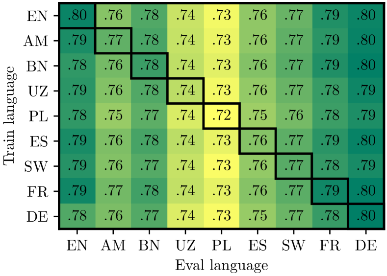
Figure 3: Performance (suite score) of Metric Learner with PanPhon features trained on a specific language and evaluated on another one. Diagonals show matching models and evaluation languages.

5.3 Transfer Between Languages

Recall from Section 3.3 that there are multiple feature types that can be used for our phonetic word embedding model: orthographic characters, IPA characters and articulatory feature vectors. It is not surprising, that the textual characters as features provide little transferability when the model is trained on a different language than it is evaluated on. The transfer between languages for a different model type, shown in Figure 3, demonstrates that not all languages are equally challenging. Furthermore, the PanPhon features appear to be very useful for generalizing across languages. This echoes the findings of Li et al. (2021), who also break down phones into articulatory features to share information across phones (including unseen phones).

5.4 Embedding Topology Visualization

The differences between feature types in Table 2 may not appear very large. However, closer inspection of the clusters in the embedding space in Figure 4 reveals, that using the PanPhon articulatory feature vectors or IPA features yields a vector space which resembles one induced by the articulatory distance the most. This is in line with the fact that $A$ (articulatory distance, Section 3.3.1) is calculated using PanPhon features and we explicitly use them to supervise the model.

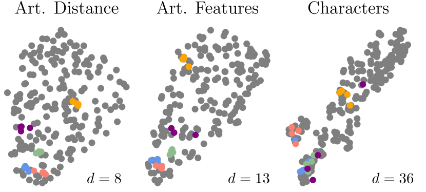
Figure 4: T-SNE projection of the articulatory distance and embedding spaces from the metric learning models with articulatory or character features. Each point corresponds to one English word. Differently coloured clusters were selected in the articulatory distance space and highlighted in other spaces. Numbers show average distance within the clusters normalized with average distance between points (unitless).

5.5 Dimensionality and Train Data Size

Through our experiments, we relied on 300-dimensional embeddings. However, this choice was motivated by the comparison to other word embeddings. Now we examine how the choice of dimensionality, keeping all other things equal, affects individual task performance. The results in Figure 5 (top) show that neither too small nor too large a dimensionality is useful for solving the proposed tasks. Furthermore, there seems to be little interaction between the task type and dimensionality. As a result, model ranking based on each task is very similar which yields Spearman and Pearson correlations of $0.61$ and $0.79$, respectively.

A natural question is how data-intensive the proposed metric learning method is. For this, we constrained the training data size and show the results in Figure 5 (bottom). Similarly to changing the dimensionality, the individual tasks react to changing the training data size without an effect of the task variable. However, the Spearman and Pearson correlations are only $0.64$ and $0.65$, respectively.

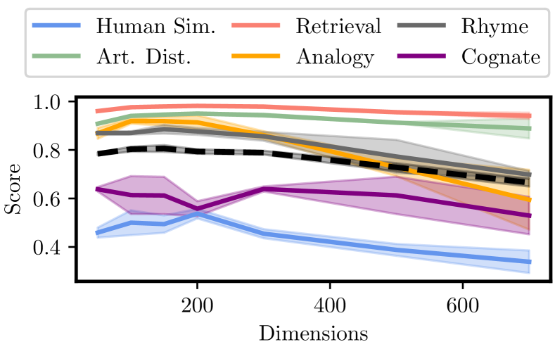
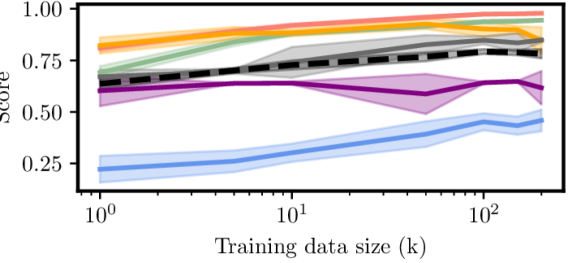
Figure 5: Task performance for Metric Learner with varying dimensionality (top) and varying training data size (bottom) with PanPhon features. Colour bands show 95% confidence intervals from t-distribution.

6 Embeddings and the Field of Phonology

Phonological features, especially articulatory features, have played a strong role in phonology since Bloomfield (1993) and especially since the work of Prague School linguists like Trubetskoy (1939) and Jakobson et al. (1951). The widely used feature set employed by PanPhon originates in the monumental Sound Pattern of English or SPE Chomsky and Halle (1968). The assumption in that work is that there is a universal set of discrete phonological features and that all speech sounds in all languages consist of vectors of these features. The similarity between these feature vectors should capture the similarity between sounds. This position is born out in our results. These features encode a wealth of knowledge gained through decades of linguistic research on how the sound systems of languages behave, both synchronically and diachronically. While there is evidence that phonological features are emergent rather than universal Mielke (2008), these results suggest that they can nevertheless contribute robustly to computational tasks. See Appendix C for a list of NLP tasks where phonetic word embeddings may be useful.

7 Future Work

After having established the standardized evaluation suite, we wish to pursue the following:

• enlarging the pool of languages,

• including more tasks in the evaluation suite,

• contextual phonetic word embeddings,

• new models for phonetic word embeddings.

Limitations

As hinted in Section 5.1, we are doing evaluation of models that use supervision from some of the tasks during training. Specifically, the metric learning models have an advantage on the articulatory distance task. Nevertheless, the models perform well also on other, more unrelated tasks and we also provide models without this supervision.

Another limitation of our work is that we train on phonemic transcriptions, which cannot capture finer grained phonetic distinctions. Phonemic distinctions may be sufficient for applications such as rhyme detection, but not for tasks such as phone recognition or dialectometry.

Finally, we do not make any distinction between training and development data. This is for a practical reason because some of the methods we use for comparison are not open embeddings and need to see all concerned words during training.

Appendix A Reproducibility Details

For the multi-layer perceptron for rhyme and cognate classification, we use the MLP class from scikit-learn (Pedregosa et al., 2011, v1.2.1) with hidden layer sizes of 50, 20 and 10 and other parameter defaults observed.

Compute resources.

The most compute-consuming tasks were training the Metric Learner and Triplet Margin, which took $\nicefrac{{1}}{{4}}$ and $2$ hours on GTX 1080 Ti, respectively. Overall for the research presented in this paper, we estimate 100 GPU hours.

Lexical word embeddings.

The BERT embeddings were extracted as an average across the last layer. The INSTRUCTOR embeddings were used with the prompt Represent the word for sound similarity retrieval: For BPEmb and fastText, we used the best models (highest training data) and dimensionality of 300.

Model details.

The metric learner uses bidirectional LSTM with 2 layers, hidden state size of 150 and dropout of 30%. The batch size is 128 and the learning rate is $10^{-2}$. The autoencoder follows the same hyperparameters both for the encoder and decoder. The difference is its learning size, $5\times 10^{-3}$, which was chosen empirically.

Appendix B Phonetic Language Modeling

As a negative result, we describe here our model which did not perform well on our suit of tasks in contrast to others. A common way of learning word embeddings as of recent is to train on the masked language model objective, popularized by BERT (Devlin et al., 2019). We input PanPhon features into several successive Transformer (Vaswani et al., 2017) encoder layers and a final linear layer that predicts the masked phone. We prepend and append [CLS] and [SEP] tokens, respectively, to the phonetic transcriptions of each word, before we look up each phone’s PanPhon features. We use [CLS] pooling–taking the output of the Transformer corresponding to the first token–to extract a word-level representation. Unlike BERT, we do not train on the next sentence prediction objective, nor do we add positional embeddings. In addition, we do not add an embedding layer because we are not interested in learning individual phone embeddings but rather wish to learn a word-level embedding.

Appendix C What are Phonetic Word Embds. For?

Phonetic word embeddings are arguably more niche than their semantic counterparts. Nevertheless, there are still many applications were shown to benefit from this endeavor. These include:

• Cognate detection (Rama, 2016)

• Text-to-speech (Sanchez et al., 2022)

• Spelling correction (Zhang et al., 2021)

• Automatic speech recognition (Fang et al., 2020)

• Multilingual named entity recognition (Bharadwaj et al., 2016; Chaudhary et al., 2018)

Appendix D Retrieval Error Analysis

We identify two types of errors in the retrieval task for the Metric Learner model wit PanPhon features. The first one are simply incorrect neighbours with low sound similarity, such as the word carcass, whose correct neighbour is cardiss but krutick is chosen. The next group are plausible ones, such as for the word counterrevolutionary, its neighbour in articulatory distance space counterinsurgency and the retrieved word cardiopulmonary. In this case we might even say that the retrieved word is closer.

References

- Almeida and Xexéo (2019) Felipe Almeida and Geraldo Xexéo. 2019. Word embeddings: A survey. arXiv preprint arXiv:1901.09069.
- Bakarov (2018) Amir Bakarov. 2018. A survey of word embeddings evaluation methods. arXiv preprint arXiv:1801.09536.
- Batsuren et al. (2019) Khuyagbaatar Batsuren, Gabor Bella, and Fausto Giunchiglia. 2019. CogNet: A large-scale cognate database. In Proceedings of the 57th Annual Meeting of the Association for Computational Linguistics, pages 3136–3145, Florence, Italy. Association for Computational Linguistics.
- Bellet et al. (2015) Aurélien Bellet, Amaury Habrard, and Marc Sebban. 2015. Metric learning. Morgan & Claypool Publishers.
- Bengio and Heigold (2014) Samy Bengio and Georg Heigold. 2014. Word embeddings for speech recognition.
- Bharadwaj et al. (2016) Akash Bharadwaj, David R Mortensen, Chris Dyer, and Jaime G Carbonell. 2016. Phonologically aware neural model for named entity recognition in low resource transfer settings. In Proceedings of the 2016 Conference on Empirical Methods in Natural Language Processing, pages 1462–1472.
- Bloomfield (1993) Leonard Bloomfield. 1993. Language. University of Chicago Press, Chicago.
- Bojanowski et al. (2017) Piotr Bojanowski, Edouard Grave, Armand Joulin, and Tomas Mikolov. 2017. Enriching word vectors with subword information. Transactions of the association for computational linguistics, 5:135–146.
- Camacho-Collados and Pilehvar (2018) Jose Camacho-Collados and Mohammad Taher Pilehvar. 2018. From word to sense embeddings: A survey on vector representations of meaning. Journal of Artificial Intelligence Research, 63:743–788.
- Carnegie Mellon Speech Group (2014) Carnegie Mellon Speech Group. 2014. The Carnegie Mellon Pronouncing Dictionary 0.7b. release 0.7b.
- Chaudhary et al. (2018) Aditi Chaudhary, Chunting Zhou, Lori Levin, Graham Neubig, David R Mortensen, and Jaime G Carbonell. 2018. Adapting word embeddings to new languages with morphological and phonological subword representations. arXiv preprint arXiv:1808.09500.
- Chomsky and Halle (1968) Noam Chomsky and Morris Halle. 1968. The Sound Pattern of English. Harper & Row, New York, NY.
- Conneau et al. (2020) Alexis Conneau, Kartikay Khandelwal, Naman Goyal, Vishrav Chaudhary, Guillaume Wenzek, Francisco Guzmán, Edouard Grave, Myle Ott, Luke Zettlemoyer, and Veselin Stoyanov. 2020. Unsupervised cross-lingual representation learning at scale. In Proceedings of the 58th Annual Meeting of the Association for Computational Linguistics, pages 8440–8451. Association for Computational Linguistics.
- Devlin et al. (2019) Jacob Devlin, Ming-Wei Chang, Kenton Lee, and Kristina Toutanova. 2019. BERT: Pre-training of deep bidirectional transformers for language understanding. In Proceedings of the 2019 Conference of the North American Chapter of the Association for Computational Linguistics: Human Language Technologies, Volume 1 (Long and Short Papers), pages 4171–4186.
- El-Geish (2019) Mohamed El-Geish. 2019. Learning joint acoustic-phonetic word embeddings. arXiv preprint arXiv:1908.00493.
- Fang et al. (2020) Anjie Fang, Simone Filice, Nut Limsopatham, and Oleg Rokhlenko. 2020. Using phoneme representations to build predictive models robust to asr errors. In Proceedings of the 43rd International ACM SIGIR Conference on Research and Development in Information Retrieval, page 699–708. Association for Computing Machinery.
- F.R.S. (1901) Karl Pearson F.R.S. 1901. LIII. on lines and planes of closest fit to systems of points in space. The London, Edinburgh, and Dublin Philosophical Magazine and Journal of Science, 2(11):559–572.
- Ghannay et al. (2016) Sahar Ghannay, Yannick Esteve, Nathalie Camelin, and Paul Deléglise. 2016. Evaluation of acoustic word embeddings. In Proceedings of the 1st Workshop on Evaluating Vector-Space Representations for NLP, pages 62–66.
- Grave et al. (2018) Edouard Grave, Piotr Bojanowski, Prakhar Gupta, Armand Joulin, and Tomas Mikolov. 2018. Learning word vectors for 157 languages. In Proceedings of the International Conference on Language Resources and Evaluation (LREC 2018).
- Heinzerling and Strube (2018) Benjamin Heinzerling and Michael Strube. 2018. BPEmb: Tokenization-free pre-trained subword embeddings in 275 languages. In Proceedings of the Eleventh International Conference on Language Resources and Evaluation (LREC 2018). European Language Resources Association (ELRA).
- Hu et al. (2020) Yushi Hu, Shane Settle, and Karen Livescu. 2020. Multilingual jointly trained acoustic and written word embeddings. arXiv preprint arXiv:2006.14007.
- Jakobson et al. (1951) Roman Jakobson, Gunnar Fant, and Morris Halle. 1951. Preliminaries to Speech Analysis: The Distinctive Features and their Correlates. MIT Press, Cambridge, Massachusetts.
- Kaya and Bilge (2019) Mahmut Kaya and Hasan Şakir Bilge. 2019. Deep metric learning: A survey. Symmetry, 11(9):1066.
- Kulis et al. (2013) Brian Kulis et al. 2013. Metric learning: A survey. Foundations and Trends® in Machine Learning, 5(4):287–364.
- Le and Mikolov (2014) Quoc Le and Tomas Mikolov. 2014. Distributed representations of sentences and documents. In International conference on machine learning, pages 1188–1196. PMLR.
- Li et al. (2021) Xinjian Li, Juncheng Li, Florian Metze, and Alan W Black. 2021. Hierarchical phone recognition with compositional phonetics. In Interspeech, pages 2461–2465.
- Miaschi and Dell’Orletta (2020) Alessio Miaschi and Felice Dell’Orletta. 2020. Contextual and non-contextual word embeddings: an in-depth linguistic investigation. In Proceedings of the 5th Workshop on Representation Learning for NLP, pages 110–119.
- Mielke (2008) Jeff Mielke. 2008. The emergence of distinctive features. Oxford University Press.
- Mikolov et al. (2013a) Tomas Mikolov, Kai Chen, Greg Corrado, and Jeffrey Dean. 2013a. Efficient estimation of word representations in vector space. arXiv preprint arXiv:1301.3781.
- Mikolov et al. (2013b) Tomas Mikolov, Wen-tau Yih, and Geoffrey Zweig. 2013b. Linguistic regularities in continuous space word representations. In Proceedings of the 2013 Conference of the North American Chapter of the Association for Computational Linguistics: Human Language Technologies, pages 746–751, Atlanta, Georgia. Association for Computational Linguistics.
- Mortensen et al. (2016) David R. Mortensen, Patrick Littell, Akash Bharadwaj, Kartik Goyal, Chris Dyer, and Lori Levin. 2016. PanPhon: A resource for mapping IPA segments to articulatory feature vectors. In Proceedings of COLING 2016, the 26th International Conference on Computational Linguistics: Technical Papers, pages 3475–3484, Osaka, Japan. The COLING 2016 Organizing Committee.
- Oh et al. (2022) Dongsuk Oh, Yejin Kim, Hodong Lee, H. Howie Huang, and Heuiseok Lim. 2022. Don’t judge a language model by its last layer: Contrastive learning with layer-wise attention pooling. In Proceedings of the 29th International Conference on Computational Linguistics, pages 4585–4592, Gyeongju, Republic of Korea. International Committee on Computational Linguistics.
- Parrish (2017) Allison Parrish. 2017. Poetic sound similarity vectors using phonetic features. In Thirteenth Artificial Intelligence and Interactive Digital Entertainment Conference.
- Pedregosa et al. (2011) F. Pedregosa, G. Varoquaux, A. Gramfort, V. Michel, B. Thirion, O. Grisel, M. Blondel, P. Prettenhofer, R. Weiss, V. Dubourg, J. Vanderplas, A. Passos, D. Cournapeau, M. Brucher, M. Perrot, and E. Duchesnay. 2011. Scikit-learn: Machine learning in Python. Journal of Machine Learning Research, 12:2825–2830.
- Pennington et al. (2014) Jeffrey Pennington, Richard Socher, and Christopher D Manning. 2014. GloVe: Global vectors for word representation. In Proceedings of the 2014 conference on empirical methods in natural language processing (EMNLP), pages 1532–1543.
- Rama (2016) Taraka Rama. 2016. Siamese convolutional networks for cognate identification. In Proceedings of COLING 2016, the 26th International Conference on Computational Linguistics: Technical Papers, pages 1018–1027.
- Sanchez et al. (2022) Ariadna Sanchez, Alessio Falai, Ziyao Zhang, Orazio Angelini, and Kayoko Yanagisawa. 2022. Unify and conquer: How phonetic feature representation affects polyglot text-to-speech (tts). arXiv preprint arXiv:2207.01547.
- Sharma et al. (2021) Rahul Sharma, Kunal Dhawan, and Balakrishna Pailla. 2021. Phonetic word embeddings. arXiv preprint arXiv:2109.14796.
- Su et al. (2022) Hongjin Su, Weijia Shi, Jungo Kasai, Yizhong Wang, Yushi Hu, Mari Ostendorf, Wen-tau Yih, Noah A. Smith, Luke Zettlemoyer, and Tao Yu. 2022. One embedder, any task: Instruction-finetuned text embeddings. arXiv preprint arXiv:2212.09741.
- Trubetskoy (1939) Nikolai Trubetskoy. 1939. Grundzüge der Phonologie, volume VII of Travaux du Cercle Linguistique de Prague. Cercle Linguistique de Prague, Prague.
- Vaswani et al. (2017) Ashish Vaswani, Noam Shazeer, Niki Parmar, Jakob Uszkoreit, Llion Jones, Aidan N Gomez, Łukasz Kaiser, and Illia Polosukhin. 2017. Attention is all you need. Advances in neural information processing systems, 30.
- Vitz and Winkler (1973) Paul C Vitz and Brenda Spiegel Winkler. 1973. Predicting the judged “similarity of sound” of English words. Journal of Verbal Learning and Verbal Behavior, 12(4):373–388.
- Wenzek et al. (2020) Guillaume Wenzek, Marie-Anne Lachaux, Alexis Conneau, Vishrav Chaudhary, Francisco Guzmán, Armand Joulin, and Edouard Grave. 2020. CCNet: Extracting high quality monolingual datasets from web crawl data. In Proceedings of the Twelfth Language Resources and Evaluation Conference, pages 4003–4012. European Language Resources Association.
- Yang and Jin (2006) Liu Yang and Rong Jin. 2006. Distance metric learning: A comprehensive survey. Michigan State Universiy, 2(2):4.
- Yang and Hirschberg (2019) Zixiaofan Yang and Julia Hirschberg. 2019. Linguistically-informed training of acoustic word embeddings for low-resource languages. In INTERSPEECH, pages 2678–2682.
- Zhang et al. (2021) Ruiqing Zhang, Chao Pang, Chuanqiang Zhang, Shuohuan Wang, Zhongjun He, Yu Sun, Hua Wu, and Haifeng Wang. 2021. Correcting chinese spelling errors with phonetic pre-training. In Findings of the Association for Computational Linguistics: ACL-IJCNLP 2021, pages 2250–2261.