Opening the random forest black box by the analysis of the mutual impact of features       

Abstract

Random forest is a popular machine learning approach for the analysis of high-dimensional data because it is flexible and provides variable importance measures for the selection of relevant features. However, the complex relationships between the features are usually not considered for the selection and thus also neglected for the characterization of the analysed samples. Here we propose two novel approaches that focus on the mutual impact of features in random forests. Mutual forest impact (MFI) is a relation parameter that evaluates the mutual association of the featurs to the outcome and, hence, goes beyond the analysis of correlation coefficients. Mutual impurity reduction (MIR) is an importance measure that combines this relation parameter with the importance of the individual features. MIR and MFI are implemented together with testing procedures that generate p-values for the selection of related and important features. Applications to various simulated data sets and the comparison to other methods for feature selection and relation analysis show that MFI and MIR are very promising to shed light on the complex relationships between features and outcome. In addition, they are not affected by common biases, e.g. that features with many possible splits or high minor allele frequencies are prefered.

The approaches are implemented in Version 0.3.0 of the R package RFSurrogates that is available at github.com/StephanSeifert/RFSurrogates.

1 Introduction

The application of the machine learning approach random forest (RF) (Breiman 2001) has become very popular for the analysis of high-dimensional data, e.g. generated in genomics (X. Chen and Ishwaran 2012) and metabolomics (T. Chen et al. 2013) experiments or genome-wide association studies (GWAS) (Nicholls et al. 2020). The reason for this popularity are specific advantages over other methods, such as the flexibility in terms of input and output variables, since both quantitative and qualitative variables can be used to build classification, regression (Strobl, Malley, and Tutz 2009) and survival models (Ishwaran et al. 2011). Another advantage is the ability to generate variable importance measures (VIMs) that are utilized to select the relevant features for parsimonious prediction models or to identify and interpret differences between the samples.
The most common VIMs are the permutation importance and the impurity importance, so called since it is calculated from the impurity gain that the variable contributes to the random forest. Another importance measure is minimal depth, which is based on the position of the variables in the decision trees (Ishwaran et al. 2010). Minimal depth and the impurity importance, however, are known to be biased in favour of features with many categories (Strobl et al. 2007) and high category frequencies (K. K. Nicodemus 2011), which is particularly important in GWAS (Boulesteix et al. 2012). Since it is not affected by these biases, the permutation importance has been preferred and various selection techniques based on this importance measure have been developed (Szymczak et al. 2016; Janitza, Celik, and Boulesteix 2018; Kursa and Rudnicki 2010) and compared (Degenhardt, Seifert, and Szymczak 2019). A few years ago, a corrected, unbiased impurity importance measure, the actual impurity reduction (AIR), was introduced (Nembrini, König, and Wright 2018). AIR is computed faster than the permutation importance, which is why this importance measure is very useful for application to high-dimensional data.
All of the RF based importance measures are affected by the correlation structure of the features (Kristin K. Nicodemus et al. 2010), and conditional variable importance has been proposed to determine the corrected, individual impact of the features (Strobl et al. 2008; Debeer and Strobl 2020). We have taken a different approach to this issue because we think that the relations between the features should be included into the analysis treating them as interacting components. Therefore, we have deliberately included feature relations to improve variable importance calculation, the power of feature selection and interpretation of differences between samples (Seifert, Gundlach, and Szymczak 2019). We have achieved this by the exploitation of surrogate variables that have been introduced to compensate for missing values in the data, representing the features that can replace another feature in a split as best as possible (Breiman et al. 1984).
Based on surrogate variables, we developed Surrogate Minimal Depth (SMD), an importance measure that incorporates surrogate variables into the concept of minimal depth, and mean adjusted agreement, a relation parameter that is determined by the split agreement of the features across the random forest. Since this relation parameter considers the mutual impact of the features on the random forest model, this parameter goes beyond the analysis of ordinary correlation coefficients enabling a comprehensive analysis of the complex interplay of features and outcome. We applied this relation analysis to reveil relations between features in gene expression (Seifert, Gundlach, and Szymczak 2019), metabolomics (Wenck et al. 2022), and various spectroscopic data sets (Shakiba et al. 2022; Seifert 2020), e.g. to illuminate the interaction of drugs with proteins and lipids in living cells (Zivanovic et al. 2019). However, since both SMD and mean adjusted agreement are affected by the previously described biases, their application has so far been limited. Here we introduce two novel approaches for the analysis of feature relations and mutual importance called mutual forest impact (MFI) and mutual impurity reduction (MIR). We will show that they are not affected by these biases and compare their performance with existing approaches by applying them to different simulated data sets.

2 Materials and Methods

2.1 Random Forest

RF is an ensemble of binary decision trees for classification, regression and survival analysis (Breiman 2001). Each of these decision trees is built from a different bootstrap sample and the best split for each node is identified from randomly chosen candidate features by maximizing the decrease of impurity. The impurity reduction is usually determined by the Gini index for classification (Breiman et al. 1984), the sum of squares for regression (Ishwaran 2015) and the log-rank statistic for survival analysis (Ishwaran et al. 2008). The three important parameters of RF are ntree, the total number of decision trees, mtry, the number of randomly chosen candidate features, and min.node.size, the maximum number of samples of the terminal nodes. Since RF is based on bagging, there are out-of-bag (OOB) samples for each tree, which have not been used in the training process and therefore can be utilized to determine prediction accuracy and variable importance.

2.2 Impurity importance

The impurity importance is based on the decrease of impurity determined by the difference of a node’s impurity and the weighted sum of the child node’s impurities. To determine the importance of a feature, the sum of all impurity decrease measures of the nodes based on this feature is divided by the number of trees. The impurity importance is biased in favour of features with many possible split points because they have a higher probability to be randomly suitable for the intended distinction (Strobl et al. 2007; Wright, Dankowski, and Ziegler 2017). In addition, features with the same number of categories but different category frequencies are biased as well (K. K. Nicodemus 2011), which is crucial for genetic analyses because single-nucleotide polymorphisms (SNPs) with high minor allele frequencies (MAF) are favoured (Boulesteix et al. 2012). In order to correct this bias, Nembrini, König, and Wright (2018) applied a modified approach of Sandri and Zuccolotto (2008) to calculate the AIR of each feature $X_{i}$ by the difference between the VIM and the VIM of a permuted version of itself:

$$\widehat{AIR_{X_{i}}}=\widehat{VIM_{X_{i}}}-\widehat{VIM_{X_{i,perm}}}$$

2.3 Surrogate variables for relation analysis

Surrogate variables were introduced by Breiman et al. (1984) for the compensation of missing values. The basic idea is that in addition to the primary splits of the decision trees in RF, alternative splits are determined based on other features of the data that can replace the primary split as best as possible. For the selection of the predefined number s of surrogate splits, the surrogates with the highest values for the adjusted agreement adj are chosen. This parameter is calculated for the primary split p and the possible surrogate q utilizing the agreement $n_{surr}$, which is determined by the number of samples that are assigned to the same daughter nodes. It is defined by

$$adj(p,q)=\frac{n_{surr}-n_{maj}}{n_{total}-n_{maj}}$$

where $n_{total}$ is the total number of samples at the respective node and $n_{maj}$ is the number of correct assignments when all samples are assigned to the daughter node with the larger number of samples, also called the majority rule. Note that surrogate variables are only chosen when the adjusted agreement is higher than 0 meaning that the surrogate split has to outperform the majority rule. This can result in less than s surrogate splits for individual nodes.
For the analysis of the variable relations of $X_{j}$ to $X_{i}$, all nodes with primary split variable $X_{i}$ are considered and the mean adjusted agreement $M_{X_{i}X_{j}}$ is defined by

$$M_{X_{i}X_{j}}=\frac{\sum_{n=1}^{|nodes(X_{i}X_{j})|}agree(p_{n}^{X_{i}},q_{n}^{X_{j}})}{|nodes(X_{i})|}$$

with $p_{n}^{X_{i}}$ and $q_{n}^{X_{j}}$ denoting the primary split based on variable $X_{i}$ and the surrogate split on variable $X_{j}$ of the node n and $nodes(X_{i})$ denoting the total number of nodes based on $X_{i}$. Related features can subsequently be selected by a threshold adjusted by a user defined factor t (default for t is 5).

2.4 Mututal forest impact (MFI)

Inspired by Nembrini, König, and Wright (2018), we developed an unbiased approach for the analysis of variable relations based on surrogate variables. For this purpose, pseudo data Z, which is uninformative but shares the structure of the original data X, is generated by the permutation of the features across observations. Thus Z contains as many permuted variables p as X. Subsequently, the mean adjusted agreement of the features is determined for both, X and Z and the novel relation parameter MFI is defined by

$$\widehat{MFI_{X_{i},X_{j}}}=\widehat{M_{X_{i},X_{j}}}-\widehat{M_{Z_{i},Z_{j}}}$$

Just as for the mean adjusted agreement, a value of 1 for the MFI of two features corresponds to an exact agreement of their impact on the random forest model.

2.5 Mutual impurity reduction (MIR)

Not only the relation parameter, but also the importances obtained by SMD are biased. For this reason, we define the novel, unbiased importance measure MIR that does not evaluate the features individually but also considers the relations between them. MIR is the sum of the AIR of the individual feature and the AIR of the other features multiplied by the corresponding relation parameter MFI:

$$\widehat{MIR_{X_{i}}}=\widehat{AIR_{X_{i}}}+\sum_{j}^{p}\widehat{MFI_{X_{i},X_{j}}}\cdot\widehat{AIR_{X_{j}}}$$

2.6 Testing procedures

Also inspired by Nembrini, König, and Wright (2018), statistical testing procedure are performed to select relevant and related parameters and the following null hypotheses are tested:

$$H_{0}:MFI_{X_{i},X_{j}}\leq 0$$

$$H_{0}:MIR_{X_{i}}\leq 0$$

For this, the respective importance and relation values are tested against a null distribution. This null distribution is obtained by zero and negative values, which are mirrored to obtain the corresponding positive values, as proposed by Janitza, Celik, and Boulesteix (2018). However, for this approach to be validly applied, there must be a sufficient number of negative values and thus a sufficient number of features p. Because of this, we developed alternative, permutation-based approaches to obtain the null distributions for important and related features. For the selection of related features in MFI, the permuted relations $\widehat{M_{Z_{i}}}$ are utilized. Since they only contain zero and positive values, the null distribution is completed similarly as in Janitza, Celik, and Boulesteix (2018): The non-zero values are mirrored to obtain the respective negative values of the distribution. For the selection of important features in MIR, the permuted relations $\widehat{M_{Z}}$ are multiplied by permuted values of AIR. This process is repeated multiple times to determine enough values to describe the null distribution sufficiently.

2.7 Simulation studies

2.7.1 Bias of importance and relation measures

In order to study the bias of the SMD importance and relation analysis, we simulated two simple null scenarios meaning that none of the simulated variables is associated with the outcome. For both, the sample size was set to 100 and the simulation was replicated 1000 times. As in Nembrini, König, and Wright (2018), the outcomes for classification, regression and survival analyses were generated from a binomial distribution with a probability of 0.5, a standard normal distribution and an exponentially distributed survival ($\lambda$ = 0.5) and censoring time ($\lambda$ = 0.1), respectively.
AIR, SMD importance and relation analysis, as well as the new approaches MFI and MIR were applied to the simulated data utilizing RF with 100 trees, an mtry of 3 and a minimal node size of 1. Furthermore, for SMD, MFI and MIR 3 surrogates s were determined in each split. The variables of the two scenarios were simulated as follows:

Null scenario A: Increasing number of expression possibilities:

Inspired by Nembrini, König, and Wright (2018), nine nominal variables $X_{1}$,…$X_{9}$ with 2, 3, 4, 5, 6, 7, 8, 10 and 20 categories were generated from a uniform distribution and one continuous variable $X_{10}$ from a standard normal distribution.

Null scenario B: Increasing minor allel frequency:

As in Nembrini, König, and Wright (2018), ten variables $X_{1}$,…$X_{10}$ with minor allele frequencies of 0.05, 0.10, 0.15, 0.20, 0.25, 0.30, 0.35, 0.40, 0.45, 0.50 from a binomial distribution were simulated.

2.7.2 Correlation Study

To evaluate the selection of variables in the presence of correlations, a simulation study from Seifert, Gundlach, and Szymczak (2019) was carried out. The quantitative outcome $Y$ is dependent on 6 relevant variables $X_{1}$, …, $X_{6}$ that were, just like three non-relevant, outcome-independent variables $X_{7}$, …, $X_{9}$, sampled from a standard normal distribution N(0,1):

$$Y=X_{1}+X_{2}+X_{3}+X_{4}+X_{5}+X_{6}+\epsilon$$

The noise $\epsilon$ followed a N(0, 0.2) distribution. In addition, 10 correlated variables (denoted as c$X_{1}$, c$X_{2}$, c$X_{3}$, c$X_{7}$, c$X_{8}$, c$X_{9}$) were generated for each of $X_{1}$, $X_{2}$, $X_{3}$, $X_{7}$, $X_{8}$ and $X_{9}$ utilizing the simulateModule function of the R package WGCNA. (Langfelder and Horvath 2008) Strong correlations (0.9) were used for $X_{1}$ and $X_{7}$, medium correlations (0.6) for $X_{2}$ and $X_{8}$, and low correlations (0.3) for $X_{3}$ and $X_{9}$. Furthermore, to reach a total number of $p_{1}$ = 1000 variables, additional independent, non-correlated variables (ncV) were simululated using a standard normal distribution. We will denote the variables $X_{1}$, …, $X_{6}$ as well as c$X_{1}$, c$X_{2}$ and c$X_{3}$ as relevant and the other variables as non-relevant. For a graphical summary of the simulation please refer to the supplementary information in Seifert, Gundlach, and Szymczak (2019).
We simulated data for 100 individuals, generated 50 replicates and applied the importance measures and feature selection approaches AIR, SMD and MIR utilizing random forests with 1000 trees, an mtry of 177 ($\widehat{=}$ $p_{1}^{(3/4)}$), and a minimal node size of 1. For AIR and MIR, the p-value thresholds 0.001, 0.01 and 0.05 and for SMD and MIR s values of 5, 10, 20 and 100 were used.
In order to compare type I error rates, we also simulated a null scenario with 1000 independent predictor variables from a standard normal distribution and an independent binary outcome. 50 replicates for 50 cases and 50 controls were simulated and AIR, MIR and SMD were applied with the same parameters as above. Type I error rates were subsequently estimated by the division of selected variables and the total number of predictor variables.

2.7.3 Realistic Study

For the comparison of the feature selection approaches under realistic correlation structures, gene expression data sets were simulated as in Seifert, Gundlach, and Szymczak (2019) and Degenhardt, Seifert, and Szymczak (2019) utilizing the R package Umpire (Zhang, Roebuck, and Coombes 2012) and a realistic covariance matrix. The covariance matrix was generated from an RNA-microarray dataset of breast cancer patients with $p_{2}$ = 12 592 genes obtained from The Cancer Genome Atlas (Network CGA, 2012). A multivariate normal distribution for a 12 592-dimensional random vector with a mean vector of zeroes was applied to obtain gene expression values for cases and controls. For the cases, 25 variables for each effect size from the set {${-2,-1,-0.5,0.5,1,2}$} were randomly chosen and the means of the variables were increased accordingly. The other variables and the covariance matrix were the same for cases and controls. Two data sets with 100 controls and 100 cases were simulated for each set of 150 causal variables and the whole process including random selection of causal variables was repeated 50 times.
As in Seifert, Gundlach, and Szymczak (2019), we estimated the evaluation criteria stability, classification error, empirical power and false positive rate (FPR) for the comparison of the performance of AIR, MIR and SMD. The approaches were applied using random forests with 5000 trees, an mtry of 1188 ($\widehat{=}$ $p_{2}^{(3/4)}$), and a minimal node size of 1. For AIR and MIR, a p-value threshold of 0.01 and for SMD and MIR s values of 50, 100, 200 and 500 were used.
Stability was determined by the Jaccard’s index (He and Yu 2010), the ratio of the length of the intersection and the length of the union of the two sets of selected variables. The classification error was determined using each of the two data sets of each replicate to select variables, on which RF models with the same parameters as for the feature selection were trained. The other data set was subsequently used as validation set and the mean classification error was calculated for each pair. The empirical power was determined separately for each absolute effect size by the fraction of correct selections among all replicates. To determine the FPR, the null variables were defined differently for each replicate characterized by other causal variables. Since variables at least moderately correlated to causal variables are of interest as well, only non-causal and non-correlated variables (correlation coefficient < 0.2) were defined as null variables. The FPR was calculated by dividing the number of selected null variables by the total numbers of null variables.

3 Results

3.1 Simulation studies

3.1.1 Bias of relation measures

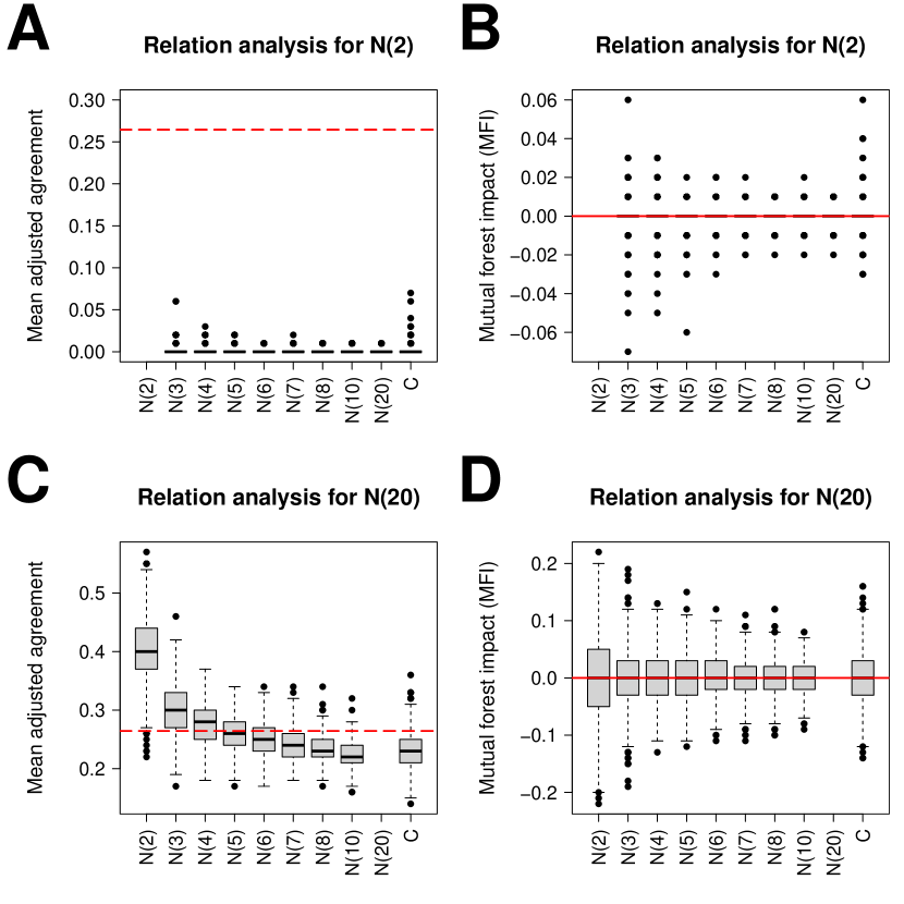
Figure 1: Null scenario A (classification): Relation analysis based on mean adjusted agreement (A+C) and MFI (B+D) for the nominal variables with 2 (A+B) and 20 (C+D) categories. The dashed line shows the threshold for the selection of related variables and a relation value of 0 for mean adjusted agreement (t=5) and MFI, respectively. The relations of the other variables are shown in the Supplementary Figures S1 and S2.

The classification results for the null scenario with increasing number of expression possibilities (null scenario A) are shown in Figure 1. The mean adjusted agreement is 0 or very close to 0, when the relations of the variable with 2 categories is analysed (Fig. 1A). Since all these values are below the threshold, no variable is falsely selected here. However, this does not apply to the relation analysis of the variable with 20 categories (Fig. 1C). Because this variable has much more expression possibilities, it shows increasing values for the mean adjusted agreement as the number of categories decrease. For the variable with only 2 categories, quite high values of approximately 0.4 are obtained resulting in a very frequent false selection of the relation between these two variables. It is obvious that, similar as for the importance analysis (Strobl et al. 2007), variables with many categories are favoured in the relation analysis, especially when relations to variables with low numbers of categories are analysed. MFI, the novel approach for relation analysis, does not show this bias, since all values for both, the variable with 2 and 20 categories, are located around 0 (Fig. 1B+D). For the latter, however, the variance increases for variables with lower numbers of categories.
Figure 2 shows the results for the analysis of increasing MAF. The mean adjusted agreement of variables with higher MAF is generally higher for the relation analysis of both, the variable with a low MAF of 0.05 (Fig. 2A) and the variable with a high MAF of 0.5 (Fig. 2C). Consequently, relations of variables with high MAF are falsely selected more frequently. The MFI is not influenced by the MAF in the same way, because all variables show values around 0 for both variables (Fig. 2B+D). However, the variance increases for variables with higher MAF.
The bias analysis of mean adjusted agreement and MFI, which is shown here for a classification outcome, are also reflected in the regression and survival analyses (see Supplementary Figures S5-S12).

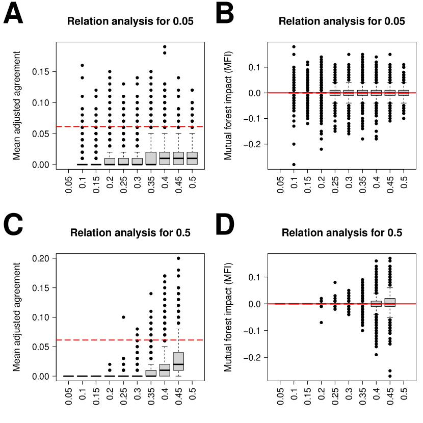
Figure 2: Null scenario B (classification): Relation analysis based on mean adjusted agreement (A+C) and MFI (B+D) for the variables with minor allele frequencies of 0.05 (A+B) and 0.5 (C+D). The dashed line shows the threshold for the selection of related variables and a relation value of 0 for mean adjusted agreement (t=5) and MFI, respectively. The relations of the other variables are shown in the Supplementary Figures S3 and S4.

3.1.2 Bias of importance measures

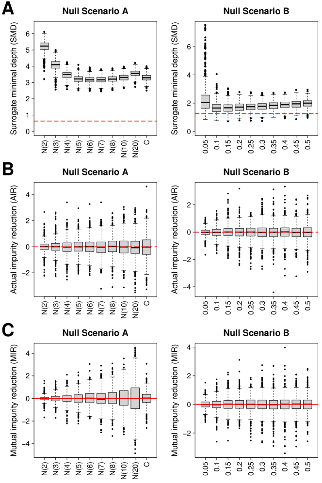
Figure 3: Variable importances for null scenarios (classification): Results of SMD (A), AIR (B), and MIR (C) in null scenario A (left) and B (right). The dashed line shows the threshold for the feature selection and an importance value of 0 for SMD (t=5) and AIR and MIR, respectively. Note that low SMD values correspond to important features.

The results for the importance analyses for both null scenarios are shown in Figure 3. SMD shows importance scores dependent on the number of categories: (Fig. 1A left) Variables with low numbers of categories have high values for SMD corresponding to low importances, while variables with high numbers of categories seem more important because they have lower SMD values. Hence, SMD shows the same bias as other importance measures favouring variables with many categories (Strobl et al. 2007). MIR, just like AIR, does not show this bias (Fig. 3B+C left). However, the well-known property of higher variances for variables with higher numbers of categories can be observed for AIR (Nembrini, König, and Wright 2018). For MIR, this influence is even more evident.
SMD is also influenced by the MAF showing different importance values for variables with different MAF and consequently also different numbers of false selections (Fig. 1A right). For AIR and MIR, this bias is not observed. However, as expected from Nembrini, König, and Wright (2018), the variance of the AIR increases towards higher MAF. For MIR, the same property is apparent.

3.1.3 Correlation Study

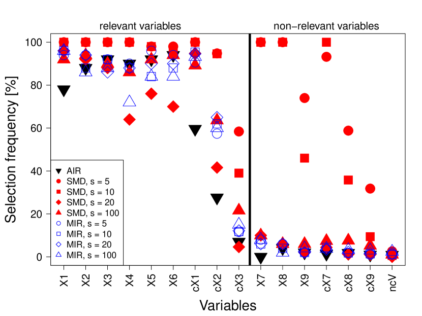
Figure 4: Results of the correlation study utilizing different numbers of surrogate variables (SMD and MIR) and a p-value thresholds of 0.01 (AIR and MIR). For the basic variables, ($X_{1}$ – $X_{9}$) the selection frequencies are averaged across all 50 replicates, whereas for the six groups of correlated variables, (c$X_{1}$ – c$X_{3}$ and c$X_{7}$ – c$X_{9}$) as well as the non-causal variables (ncV) the average frequencies across all replicates and variables in the respective group are shown.

The selection frequencies of SMD, AIR and MIR for the different variables and variable groups are shown in Figure 4. SMD with 5 and 10 surrogate variables (red circles and squares) shows the highest selection frequencies for all relevant variables reaching 100% for $X_{1}$, $X_{2}$, $X_{3}$, $X_{4}$ and c$X_{1}$, more than 90% for $X_{5}$, $X_{6}$ and c$X_{2}$ as well as between 35 and 60% for c$X_{3}$. However, also the correlated non-relevant variables are frequently selected here, $X_{7}$ and $X_{8}$ even always. For SMD with higher numbers of surrogate variables (red diamonds and triangles) and for MIR, (blue symbols) the selection frequencies are mostly higher than 80% for $X_{1}$ to $X_{6}$ and c$X_{1}$. An exception are the frequencies of SMD with s = 20 for $X_{4}$ to $X_{6}$ and MIR with s = 100 for $X_{4}$ that are between 60 and 80%. For c$X_{2}$ and c$X_{3}$, MIR shows selection frequencies of around 60 and 15% independent from the number of surrogate variables used, while the frequencies of SMD are much more dependent on this parameter. This is also evident for the non-relevant variables, as MIR has similarly low frequencies, while SMD is characterized by higher, more variable frequencies.
For AIR (black triangle in Fig. 4), selection frequencies are lower than for MIR and SMD (red and blue symbols) when correlations between the variables exist. This applies for the causal variables, where the values for $X_{1}$, c$X_{1}$ and c$X_{2}$ are at around 80, 60 and 25%, respectively, and for the non-causal variables that show values at or close to zero for all variables.
A comparison of different p-value thresholds for MIR and AIR shows that the used value of 0.01, the default value of AIR, is reasonable (Supplementary Figures S15). The comparison of the selection of related variables by SMD and MIR shows no significant differences, which is due to the fact that this study does not use variables that exhibit the biases outlined above (Supplementary Figures S16).
From the correlation study, it can be concluded that MIR is more powerful for correlated variables than AIR and less sensitive to changes in the number of surrogate variables used than SMD. However, too high values for s lead to an increased false positive rate, which is apparent for the non-causal variables (ncV) in Fig. 4 and the null scenario (Supplementary Figures S17).

3.1.4 Realistic Study

Figure 5 displays the results for the realistic simulation study. MIR and SMD both show increasing empirical powers as the number of surrogate variables s increases (blue and red symbols in Fig. 5B). However, for each value of s, MIR has slightly higher empirical powers for variables with low effect sizes (|0.5|). For the medium effect size of |1|, this is only apparent for s = 50 because empirical powers of 1 are achieved for higher values of s (blue and red circles in Fig. 5B). The stability shows an opposite influence of this parameter, since high values are obtained when s is low and vice visa. When 100 and 200 surrogate variables are used, SMD shows higher stabilities than MIR almost reaching 0.8 and 0.4, respectively (squares and diamonds in Fig. 5A).
AIR shows similar empirical powers as SMD with s = 100 (red square and black triangle in Fig 5B). However the stability is much lower and, just as in SMD and MIR with s = 500 (red and blue triangles in Fig 5A), the false positive rate is higher than 0.

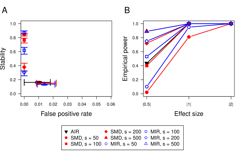
Figure 5: Results of the realistic study: Comparison of the performance of AIR, MIR (p-value threshold for both: 0.01) and SMD using different numbers of surrogates. Median, as well as the interquartile range over all 50 replicates for stability and false positive rate (A) and median frequencies of the empirical power for the different effect sizes (B) are shown. The classification error is 0 for all investigations.

4 Discussion and conclusion

In this study, we introduced two novel approaches that are based on surrogate variables in random forest: Mutual forest impact (MFI) for relation analysis and mutual impurity reduction (MIR) as a feature selection approach considering feature relations. We demonstrated that both, MFI and MIR are not biased regarding variables with different numbers of categories and category frequencies. They can be applied in random forest classification, regression and survival analyses.
Inspired by the feature selection based on the actual impurity reduction (AIR) (Nembrini, König, and Wright 2018), we combined MFI and MIR with the testing procedure of Janitza, Celik, and Boulesteix (2018) to estimate p-values for the selection of related and important features, respectively. The comparison of AIR and MIR demonstrated that the inclusion of feature relations for selection is advantageous because a higher stability and power is obtained. The comparison with SMD showed lower probabilities of false selections and a smaller sensitivity to changes of the crucial parameter s, which determines the number of surrogates used (Seifert, Gundlach, and Szymczak 2019). Since this parameter is crucial to achieve an optimal compromise between high power and low false selections, a smaller sensitivity to this parameter enables the usage of higher values resulting in a higher power. However, we have shown that even for MIR, too high values for s should not be used and additional analyses of data with different numbers of features and correlation structures are needed to find optimal values for the specific data types. We currently recommend for high-dimensional settings to use 1 to 2% of the total variables as utilized number of surrogate variables in combination with a p-value threshold of 0.01.
Due to the non-existing biases, a wide application of MFI and MIR to data with different distributions, such as continuous (e.g. metabolomics, proteomics, isotopolomics), categorical (genomics) or proportional data (epigenomics) is possible. MFI is especially promising for the relation analysis of features across different data sets, in which, in addition to different omics levels, even phenotypic information and clinical biomarkers could be included. In addition omics data could be combined with data from spectroscopic experiments, for example based on infrared, Raman or X-ray radiation.
MFI allows the selected features to be divided into groups with similar impact on the random forest model. These groups and the feature relations they are based on could be linked to known biological interactions, for example in metabolic pathways, in a similar way as recently conducted with SMD (Wenck et al. 2022). In subsequent analyses, the groups of related features could be utilized instead of individual features to robustly identify samples with specific properties, e.g. by applying pathway-based approaches (Seifert et al. 2020). In addition, based on MFI, subgroups of samples could be revealed by the identification of subgroup specific features. The identified subgroups could then be applied for the characterization of the analysed samples and to improve the machine learning model (Goel et al. 2020).
In conclusion, the novel approaches MIR and MFI are very promising for the powerful selection of relevant features and the comprehensive investigation of the complex connection between features and outcome in omics, multi-omics, and other data.

Funding

The research for this original paper was funded by the Deutsche Forschungsgemeinschaft (DFG, German Research Foundation) under Germany’s Excellence Strategy – EXC 2176 ‘Understanding Written Artefacts: Material, Interaction and Transmission in Manuscript Cultures’, project no. 390893796. The research was conducted within the scope of the Centre for the Study of Manuscript Cultures (CSMC) at Universität Hamburg.

References

reBoulesteix, A.-L., A. Bender, J. Lorenzo Bermejo, and C. Strobl. 2012. “Random Forest Gini Importance Favours SNPs with Large Minor Allele Frequency: Impact, Sources and Recommendations.” Brief. Bioinform. 13 (3): 292–304. https://doi.org/10.1093/bib/bbr053.

preBreiman, Leo. 2001. “Random Forests.” Mach. Learn. 45 (1): 5–32. https://doi.org/10.1023/A:1010933404324.

preBreiman, Leo, Jerome Friedman, Charles J. Stone, and R. A. Olshen. 1984. Classification and Regression Trees. Taylor & Francis.

preChen, Tianlu, Yu Cao, Yinan Zhang, Jiajian Liu, Yuqian Bao, Congrong Wang, Weiping Jia, and Aihua Zhao. 2013. “Random Forest in Clinical Metabolomics for Phenotypic Discrimination and Biomarker Selection.” Evid. Based Complementary Altern. Med. 2013: 1–11. https://doi.org/10.1155/2013/298183.

preChen, Xi, and Hemant Ishwaran. 2012. “Random Forests for Genomic Data Analysis.” Genomics 99 (6): 323–29. https://doi.org/10.1016/j.ygeno.2012.04.003.

preDebeer, Dries, and Carolin Strobl. 2020. “Conditional Permutation Importance Revisited.” BMC Bioinform. 21 (1): 307. https://doi.org/10.1186/s12859-020-03622-2.

preDegenhardt, Frauke, Stephan Seifert, and Silke Szymczak. 2019. “Evaluation of Variable Selection Methods for Random Forests and Omics Data Sets.” Brief. Bioinform. 20 (2): 492–503. https://doi.org/10.1093/bib/bbx124.

preGoel, Karan, Albert Gu, Yixuan Li, and Christopher Ré. 2020. “Model Patching: Closing the Subgroup Performance Gap with Data Augmentation.” arXiv:2008.06775, August. https://arxiv.org/abs/2008.06775.

preHe, Zengyou, and Weichuan Yu. 2010. “Stable Feature Selection for Biomarker Discovery.” Comput. Biol. Chem. 34 (4): 215–25. https://doi.org/10.1016/j.compbiolchem.2010.07.002.

preIshwaran, Hemant. 2015. “The Effect of Splitting on Random Forests.” Mach. Learn. 99 (1): 75–118. https://doi.org/10.1007/s10994-014-5451-2.

preIshwaran, Hemant, Udaya B. Kogalur, Eugene H. Blackstone, and Michael S. Lauer. 2008. “Random Survival Forests.” Ann. Appl. Stat. 2 (3). https://doi.org/10.1214/08-AOAS169.

preIshwaran, Hemant, Udaya B. Kogalur, Xi Chen, and Andy J. Minn. 2011. “Random Survival Forests for High-Dimensional Data.” Stat. Anal. Data Min. 4 (1): 115–32. https://doi.org/10.1002/sam.10103.

preIshwaran, Hemant, Udaya B. Kogalur, Eiran Z. Gorodeski, Andy J. Minn, and Michael S. Lauer. 2010. “High-Dimensional Variable Selection for Survival Data.” J. Am. Stat. Assoc. 105 (489): 205–17. https://doi.org/10.1198/jasa.2009.tm08622.

preJanitza, Silke, Ender Celik, and Anne-Laure Boulesteix. 2018. “A Computationally Fast Variable Importance Test for Random Forests for High-Dimensional Data.” Adv. Data Anal. Classif. 12: 885–915.

preKursa, Miron B., and Witold R. Rudnicki. 2010. “Feature Selection with the Boruta Package.” J. Stat. Softw. 36 (1): 1–13. https://doi.org/10.18637/jss.v036.i11.

preLangfelder, Peter, and Steve Horvath. 2008. “WGCNA: An R Package for Weighted Correlation Network Analysis.” BMC Bioinform. 9: 559. https://doi.org/10.1186/1471-2105-9-559.

preNembrini, Stefano, Inke R König, and Marvin N Wright. 2018. “The Revival of the Gini Importance?” Bioinformatics 34 (21): 3711–18. https://doi.org/10.1093/bioinformatics/bty373.

preNicholls, Hannah L., Christopher R. John, David S. Watson, Patricia B. Munroe, Michael R. Barnes, and Claudia P. Cabrera. 2020. “Reaching the End-Game for GWAS: Machine Learning Approaches for the Prioritization of Complex Disease Loci.” Front. Genet. 11 (April): 350. https://doi.org/10.3389/fgene.2020.00350.

preNicodemus, K. K. 2011. “Letter to the Editor: On the Stability and Ranking of Predictors from Random Forest Variable Importance Measures.” Brief. Bioinform. 12 (4): 369–73. https://doi.org/10.1093/bib/bbr016.

preNicodemus, Kristin K., James D. Malley, Carolin Strobl, and Andreas Ziegler. 2010. “The Behaviour of Random Forest Permutation-Based Variable Importance Measures Under Predictor Correlation.” BMC Bioinform. 11: 110. https://doi.org/10.1186/1471-2105-11-110.

preSandri, Marco, and Paola Zuccolotto. 2008. “A Bias Correction Algorithm for the Gini Variable Importance Measure in Classification Trees.” J. Comput. Graph. Stat. 17 (3): 611–28. https://doi.org/10.1198/106186008X344522.

preSeifert, Stephan. 2020. “Application of Random Forest Based Approaches to Surface-Enhanced Raman Scattering Data.” Sci. Rep. 10 (1): 5436. https://doi.org/10.1038/s41598-020-62338-8.

preSeifert, Stephan, Sven Gundlach, Olaf Junge, and Silke Szymczak. 2020. “Integrating Biological Knowledge and Gene Expression Data Using Pathway-Guided Random Forests: A Benchmarking Study.” Edited by Luigi Martelli. Bioinformatics 36 (15): 4301–8. https://doi.org/10.1093/bioinformatics/btaa483.

preSeifert, Stephan, Sven Gundlach, and Silke Szymczak. 2019. “Surrogate Minimal Depth as an Importance Measure for Variables in Random Forests.” Bioinformatics 35 (19): 3663–71. https://doi.org/10.1093/bioinformatics/btz149.

preShakiba, Navid, Annika Gerdes, Nathalie Holz, Soeren Wenck, René Bachmann, Tobias Schneider, Stephan Seifert, Markus Fischer, and Thomas Hackl. 2022. “Determination of the Geographical Origin of Hazelnuts (Corylus Avellana L.) By Near-Infrared Spectroscopy (NIR) and a Low-Level Fusion with Nuclear Magnetic Resonance (NMR).” Microchem. J. 174 (March): 107066. https://doi.org/10.1016/j.microc.2021.107066.

preStrobl, Carolin, Anne-Laure Boulesteix, Thomas Kneib, Thomas Augustin, and Achim Zeileis. 2008. “Conditional Variable Importance for Random Forests.” BMC Bioinform. 9: 307. https://doi.org/10.1186/1471-2105-9-307.

preStrobl, Carolin, Anne-Laure Boulesteix, Achim Zeileis, and Torsten Hothorn. 2007. “Bias in Random Forest Variable Importance Measures: Illustrations, Sources and a Solution.” BMC Bioinform. 8 (1): 25. https://doi.org/10.1186/1471-2105-8-25.

preStrobl, Carolin, James Malley, and Gerhard Tutz. 2009. “An Introduction to Recursive Partitioning: Rationale, Application, and Characteristics of Classification and Regression Trees, Bagging, and Random Forests.” Psychol. Methods 14 (4): 323–48. https://doi.org/10.1037/a0016973.

preSzymczak, Silke, Emily Holzinger, Abhijit Dasgupta, James D. Malley, Anne M. Molloy, James L. Mills, Lawrence C. Brody, Dwight Stambolian, and Joan E. Bailey-Wilson. 2016. “r2VIM: A New Variable Selection Method for Random Forests in Genome-Wide Association Studies.” BioData Min. 9 (1). https://doi.org/10.1186/s13040-016-0087-3.

preWenck, Soeren, Marina Creydt, Jule Hansen, Florian Gärber, Markus Fischer, and Stephan Seifert. 2022. “Opening the Random Forest Black Box of the Metabolome by the Application of Surrogate Minimal Depth.” Metabolites 12 (1): 5. https://doi.org/10.3390/metabo12010005.

preWright, Marvin N., Theresa Dankowski, and Andreas Ziegler. 2017. “Unbiased Split Variable Selection for Random Survival Forests Using Maximally Selected Rank Statistics.” Stat. Med. 36 (8): 1272–84. https://doi.org/10.1002/sim.7212.

preZhang, Jiexin, Paul L. Roebuck, and Kevin R. Coombes. 2012. “Simulating Gene Expression Data to Estimate Sample Size for Class and Biomarker Discovery.” Int. J. Advances Life Sci. 4: 44–51.

preZivanovic, Vesna, Stephan Seifert, Daniela Drescher, Petra Schrade, Stephan Werner, Peter Guttmann, Gergo Peter Szekeres, et al. 2019. “Optical Nanosensing of Lipid Accumulation Due to Enzyme Inhibition in Live Cells.” ACS Nano 13 (8): 9363–75. https://doi.org/10.1021/acsnano.9b04001.

p