Hedging Valuation Adjustment for Callable Claims

Abstract

Darwinian model risk is the risk of mis-price-and-hedge biased toward short-to-medium systematic profits of a trader, which are only the compensator of long term losses becoming apparent under extreme scenarios where the bad model of the trader no longer calibrates to the market. The alpha leakages that characterize Darwinian model risk are undetectable by the usual market risk tools such as value-at-risk, expected shortfall, or stressed value-at-risk. Darwinian model risk can only be seen by simulating the hedging behavior of a bad model within a good model. In this paper we extend to callable assets the notion of hedging valuation adjustment introduced in previous work for quantifying and handling such risk. The mathematics of Darwinian model risk for callable assets are illustrated by exact numerics on a stylized callable range accrual example. Accounting for the wrong hedges and exercise decisions, the magnitude of the hedging valuation adjustment can be several times larger than the mere difference, customarily used in banks as a reserve against model risk, between the trader’s price of a callable asset and its fair valuation.

Keywords: financial derivatives pricing and hedging, callable asset, model risk, model calibration, hedging valuation adjustment (HVA).

Mathematics Subject Classification: 91B25, 91B26, 91B30, 91G20.

JEL Classification: D52, G13, G24, G28.

1 Introduction

Karoui, Jeanblanc-picqué, and Shreve (1998) consider a trader selling an option at a price higher than its true value, whence, in convex setups, the possibility for the trader of superhedging the option at such price. Under the name of Darwinian model risk, Albanese, Crépey, and Iabichino (2021) consider the opposite pattern where, due to the competition between banks, a trader can only sell the option at a price lower than its true value, hence losses for the bank. The latter holds unless the trader uses the true model, the good practice which should therefore be encouraged, by penalizing the trader tempted to use a wrong model. In order to quantify the above, Albanese, Bénézet, and Crépey (2022) revisit Burnett (2021); Burnett and Williams (2021)’s notion of hedging valuation adjustment (HVA) in the direction of Darwinian model risk.

However, this was only done for European claims. But Albanese, Crépey, and Iabichino (2021) showcase that for structured products with early exercise features, with a callable range accrual as feature example, the Darwinian model risk is mostly driven by delayed exercise decisions. The present paper develops the mathematics of Darwinian model risk for callable claims. Here is the story. A trader prefers to the reference fair valuation model an alternative pricing model, which renders him more competitive in valuation terms. He then closes the deal at some valuation loss (this is the first Darwinian adverse selection principle for models in Albanese, Crépey, and Iabichino (2021)), but this loss is more than compensated by systematic recalibration gains on the hedging side of the position (second Darwinian principle). But, as hedging gains are a martingale, these overall positive gains are only short to medium term view. In the long run, large losses are incurred by the bank when market conditions reveal the unsoundness of the trader’s model (corollary to the second Darwinian principle), forcing a “bad” trader, unable to react and use the fair valuation model, to call back the claim and liquidate his position at the (stopping) time $\tau_{s}$ of the extreme event. A “not-so-bad” trader, instead, would switch from the bad model to the fair valuation one at $\tau_{s}$. This trader would then readjust its hedging position in line with the prescription of the fair valuation model and keep the position up to the expiration of the product or early call according to the prescriptions of the fair valuation model. In both cases (“bad” and not-so-bad”), the profit-and-loss of the trader fails to be a martingale and an hedging valuation adjustment (HVA) needs to be charged to the client in order to restore the martingality of the thus-augmented pnl. The HVA-compensated price is right, but the hedge computed on $[0,{\tau_{s}})$ under the trader’s model is still wrong, whence unhedged risk that deserves capital. A KVA risk premium à la (Albanese, Bénézet, and Crépey, 2022) is thus added on top of the HVA.

The rest of the paper is organized as follows. The fair valuations of European and callable claims are defined in Section 2. Section 3 introduces the notion of HVA for callable claims, declined in two versions regarding the bad and the not-so-bad trader in the above. Section 4 specializes the resulting equations to a stylized version of the callable range accrual in Albanese, Crépey, and Iabichino (2021). Until this point, for simplicity of presentation, all is done in continuous time. With numerics in view, Section 5 provides a discrete-time version of Section 4, where all the equations can be implemented exactly (via formulas detailed in Section A). The numerical results are commented in Section 6.

2 Pricing Setup

Let there be given the physical probability space and a financial sub-$\sigma$-field $\mathcal{B}$ of the full model $\sigma$ algebra $\mathcal{A}$. A reference risk-neutral measure, equivalent to the restriction to $\mathcal{B}$ of the physical probability measure, is defined on $\mathcal{B}$. Our probability measure $\mathbb{Q}$ in the paper is the uniquely defined probability measure on $\mathcal{A}$, provided by Artzner, Eisele, and Schmidt (2020, Proposition 2.1), such that (i) $\mathbb{Q}$ coincides with the reference risk-neutral measure on $\mathcal{B}$ and (ii) $\mathbb{Q}$ and the physical measure coincide conditionally on $\mathcal{B}$.

We denote by $T$ the final maturity of a claim and its hedge. The risk-free asset is chosen as a numéraire. All processes are adapted to a filtration $\mathfrak{F}=(\mathfrak{F}_{t},0\leq t\leq T)$ on $(\Omega,\mathcal{A},\mathbb{Q})$, satisfying the usual conditions. All prices are modeled as semimartingales in a càdlàg version. The $(\mathfrak{F}_{t},\mathbb{Q})$ conditional probability, expectation, value-at-risk (at some given confidence level $\alpha\in(\frac{1}{2},1)$ which is fixed throughout the paper) and expected shortfall (in the tail conditional expectation sense of an expected loss given this loss exceeds its value-at-risk), are respectively denoted by $\mathbb{Q}_{t}$, $\mathbb{E}_{t}$, $\mathbb{V}a\mathbb{R}_{t}$ and $\mathbb{ES}_{t}$ (and for $t=0$ we drop the index $t$).

For any process $X$, we write: $X_{(0)}=X-X_{0}$; $X^{\theta}$, for the process $X$ stopped at (possibly random) time $\theta$.

Definition 2.1.

We call cash flow, any optional and integrable process $\mathcal{Y}$ such that $\mathcal{Y}_{0}=0$. (i) Its fair value process, $Y=va(\mathcal{Y})$, is

$$\begin{aligned} Y_{t}=\mathbb{E}_{t}\left[{\mathcal{Y}}_{{T}}-{\mathcal{Y}}_{t}\right],\,t\leq{T};\end{aligned}$$ (1)

(ii) Its fair callable value process, $Z=\widetilde{va}(\mathcal{Y})$, is

$$\begin{aligned} Z_{t}=\sup_{\tau\in\mathcal{T}^{t}}\mathbb{E}_{t}\left[\mathcal{Y}_{\tau}-\mathcal{Y}_{t}\right],\,t\leq T,\end{aligned}$$ (2)

where $\mathcal{T}^{t}$ denotes the set of all the $[t,T]$ valued $\mathfrak{F}$ stopping times.

Lemma 2.1.

For any cash flow $\mathcal{Y}$, with fair value and fair callable value processes $Y$ and $Z$: (i) $(\mathcal{Y}+Y)$ is a martingale on $[0,T]$; (ii) $(\mathcal{Y}+Z)$ is a supermartingale on $[0,T]$. Denoting by $K$ its drift, i.e. the unique nondecreasing integrable predictable process, arising from Doob’s supermartingale decomposition theorem, such that $K_{0}=0$ and $(\mathcal{Y}+Z+K)$ is a martingale on $[0,T]$, we have for any stopping time $\tau\leq T$ and deterministic time $t\leq T$ :

$$\begin{aligned} &va(K^{\tau})_{t}=(\mathcal{Y}+Z)^{\tau}_{t}-\mathbb{E}_{t}\left[(\mathcal{Y}+Z)^{\tau}_{T}\right],\\ &\;\;\;\;\;\;\;\;\;va(K^{\tau})_{0}=Z_{0}-\mathbb{E}\left[(\mathcal{Y}+Z)^{\tau}_{T}\right].\end{aligned}$$ (3)

Proof.  (i) By (1). (ii) By definition of $K$, $(\mathcal{Y}+Z+K)$ is a martingale on $[0,T]$. So is in turn $(\mathcal{Y}+Z+K)^{\tau}$, which thus has zero value. Hence

$$\begin{aligned} 0&=va((\mathcal{Y}+Z+K)^{\tau})_{t}=va((\mathcal{Y}+Z)^{\tau})_{t}+va(K^{\tau})_{t}\\ &=\mathbb{E}_{t}\left[(\mathcal{Y}+Z)^{\tau}_{T}\right]-(\mathcal{Y}+Z)^{\tau}_{t}+va(K^{\tau})_{t},\end{aligned}$$

from which we deduce the first relation in (3). Taking $t=0$ gives the second relation, as $\mathcal{Y}_{0}=0$ by Definition 2.1.  

3 HVA for Callables

Along the storyline of Section 1 and assuming zero recovery hereafter, the asset can be called back at any time for zero value by the bank. We denote respectively by ${\tau_{s}}$ and ${\tau_{e}}\in\mathcal{T}^{0}$ the model switch time and the exit time of its position (asset called and hedge liquidated) by the trader.

We denote by $\mathcal{Q}$, the cash flow promised to the trader (assumed long one position in the asset) under the callable claim covenants, and $Q$, the fair callable value process of $\mathcal{Q}$, while $q$ represents the value of the asset in the trader’s model (satisfying $q_{T}=0$, in particular). The trader hedges the callable claim through a (European) static hedge, with promised cash flow $\mathcal{P}$ (possibly rebalanced at ${\tau_{s}}$) fairly valued by $P=va(\mathcal{P})$. However, as the trader does not anticipate the model switch, the cash flow $\mathcal{P}^{calib}$ corresponding to the hedging instruments held by the trader on $[0,\tau_{s})$ may differ from $\mathcal{P}$. We assume that the trader’s model price $p$ of $\mathcal{P}^{calib}$ coincides on $[0,{\tau_{s}})$ with the fair valuation $P^{calib}$ of $\mathcal{P}^{calib}$, by continuous recalibration of his model to the latter (whereas a price $P^{calib}_{{\tau_{s}}}$ at ${\tau_{s}}$ for $\mathcal{P}^{calib}$ will not be achievable in the class of models used by the trader). We also assume that a dynamic hedging component yields to the trader a martingale wealth $h=h^{{\tau_{e}}}$. All in one, the cumulative profit and loss process of the trader is given by

$$\begin{aligned} &pnl=(\mathcal{Q}+J^{s}q+(1-J^{s})Q)^{{\tau_{e}}}_{(0)}-(\mathcal{P}+J^{s}p+(1-J^{s})P)^{{\tau_{e}}}_{(0)}-h\\ &\;\;\;\;\;\;\;\;\;-(1-J^{e})(J^{s}q+(1-J^{s})Q)_{{\tau_{e}}},\end{aligned}$$ (4)

where $J^{s}=\mathds{1}_{[0,{\tau_{s}})}$ and $J^{e}=\mathds{1}_{[0,{\tau_{e}})}$ (and $J^{s}p=J^{s}P^{calib}$). In particular,

$$\begin{aligned} &pnl_{{\tau_{e}}}-pnl_{{\tau_{e}}-}=\mathcal{Q}_{{\tau_{e}}}-\mathcal{Q}_{{\tau_{e}}-}+(J^{s}_{{\tau_{e}}}q_{{\tau_{e}}}+(1-J^{s}_{{\tau_{e}}})Q_{{\tau_{e}}})-(J^{s}_{{\tau_{e}}-}q_{{\tau_{e}}-}+(1-J^{s}_{{\tau_{e}}-})Q_{{\tau_{e}}-})\\ &\;\;\;\;\;\;\;\;\;-(\mathcal{P}_{{\tau_{e}}}-\mathcal{P}_{{\tau_{e}}-})-(J^{s}_{{\tau_{e}}}p_{{\tau_{e}}}+(1-J^{s}_{{\tau_{e}}})P_{{\tau_{e}}})+(J^{s}_{{\tau_{e}}-}p_{{\tau_{e}}-}+(1-J^{s}_{{\tau_{e}}-})P_{{\tau_{e}}-})\\ &\;\;\;\;\;\;\;\;\;-(h_{{\tau_{e}}}-h_{{\tau_{e}}-})-(J^{s}_{{\tau_{e}}}q_{{\tau_{e}}}+(1-J^{s}_{{\tau_{e}}})Q_{{\tau_{e}}})\\ &\;\;\;\;\;\;\;\;\;=-(h_{{\tau_{e}}}-h_{{\tau_{e}}-})\\ &\;\;\;\;\;\;\;\;\;+\mathcal{Q}_{{\tau_{e}}}-\mathcal{Q}_{{\tau_{e}}-}-(J^{s}_{{\tau_{e}}-}q_{{\tau_{e}}-}+(1-J^{s}_{{\tau_{e}}-})Q_{{\tau_{e}}-})\\ &\;\;\;\;\;\;\;\;\;-(\mathcal{P}_{{\tau_{e}}}-\mathcal{P}_{{\tau_{e}}-})+(J^{s}_{{\tau_{e}}-}p_{{\tau_{e}}-}+(1-J^{s}_{{\tau_{e}}-})P_{{\tau_{e}}-})-(J^{s}_{{\tau_{e}}}p_{{\tau_{e}}}+(1-J^{s}_{{\tau_{e}}})P_{{\tau_{e}}}).\end{aligned}$$ (5)

The comparison between the last two lines, where the very last term $(J^{s}_{{\tau_{e}}}p_{{\tau_{e}}}+(1-J^{s}_{{\tau_{e}}})P_{{\tau_{e}}})$ is the liquidation cash flow of the hedge, whereas we see no such term on the side of the asset, shows that the formulation (4) indeed corresponds to a call of the asset at zero recovery.

$\mathcal{Q},\mathcal{P}^{calib}$	cash flows promised to the bank on the callable asset, and on its static hedge as seen from any time $t\in[0,{\tau_{s}})$
$Q,P^{calib}$	their respective fair value processes
$\mathcal{P}^{{\tau_{s}}},\mathds{1}_{[{\tau_{s}},T]}(\mathcal{P}-\mathcal{P}_{{\tau_{s}}})$	cash flows promised to the bank on its static hedge, until ${\tau_{s}}$ and from ${\tau_{s}}$ onward, respectively
$P$	fair value process of $\mathcal{P}=\mathcal{P}^{{\tau_{s}}}+\mathds{1}_{[{\tau_{s}},T]}(\mathcal{P}-\mathcal{P}_{{\tau_{s}}})$
$q,p=P^{calib}$	trader’s price for the asset and for the cash flow $\mathcal{P}^{calib}$, where the equality holds on $[0,{\tau_{s}})$, via continuous recalibration
$\tau_{s/e}$	model switch time and exit time of the position

Table 1: Main callable HVA data.

Remark 3.1.

Accounting for a recovery rate $R\in[0,1]$, we would have an additional term $R(J^{s}_{{\tau_{e}}}q_{{\tau_{e}}}+(1-J^{s}_{{\tau_{e}}})Q_{{\tau_{e}}})$ in (5), i.e. the second line in (4) would be multiplied by $1-R$. In particular, $R=1$ would mean that the asset is liquidly sold at ${\tau_{e}}$. A recovery rate $R<1$ covers the realistic case of a structured product, which is illiquid and can only be called (as opposed to sold) by the bank, at the cost of a loss equal to a fraction $1-R$ of its value at ${\tau_{e}}$.

Note that, because of model risk, $pnl$ fails to be a martingale, as opposed to the model-risk-free version of (4) that would result from replacing $q$ by $Q$ and $p$ by $P$ there (also assuming optimal exercise so that $Q_{\tau_{e}}=0$). The HVA is a reserve imposed by the bank to the trader to cope with misvaluation model risk, so that the HVA-compensated pnl, $-pnl+{\rm HVA}_{(0)}$, is a martingale:

Definition 3.1.

The hedging valuation adjustment (${\rm HVA}$) is

$$\begin{aligned} {\rm HVA}=-va(pnl).\end{aligned}$$ (6)

Lemma 3.1.

We have ${\rm HVA}=va(\mathcal{H}+K^{{\tau_{e}}}),$ where

$$\begin{aligned} \mathcal{H}&=(\mathcal{Q}+Q)^{{\tau_{e}}}_{(0)}-(\mathcal{P}+P)^{{\tau_{e}}}_{(0)}-pnl,\end{aligned}$$ (7)

and $K$ is the drift of $(\mathcal{Q}+Q)$.

Proof.  By definition (6) of HVA and (7) of $\mathcal{H}$, we have

$$\begin{aligned} {\rm HVA}=va(-pnl)&=va(\mathcal{H}-(\mathcal{Q}+Q)^{{\tau_{e}}}_{(0)}+(\mathcal{P}+P)^{{\tau_{e}}}_{(0)})\\ &=va(\mathcal{H}+K^{\tau_{e}}-(\mathcal{Q}+Q+K)^{{\tau_{e}}}_{(0)}+(\mathcal{P}+P)^{{\tau_{e}}}_{(0)})\\ &=va(\mathcal{H}+K^{\tau_{e}})+va(-(\mathcal{Q}+Q+K)^{{\tau_{e}}}_{(0)}+(\mathcal{P}+P)^{{\tau_{e}}}_{(0)}),\end{aligned}$$

where the second term vanishes as $(\mathcal{Q}+Q+K)^{{\tau_{e}}}$ and $(\mathcal{P}+P)^{{\tau_{e}}}$ are martingales on $[0,T]$, by Lemma 2.1.  

Proposition 3.1.

We have

$$\begin{aligned} &{\rm HVA}=(J^{s}((q-Q)-(p-P)))^{\tau_{e}}+D+J^{e}D^{\prime}+va(K^{\tau_{e}}),\mbox{ where }\\ &\;\;\;\;\;\;\;\;\;\;\;\;\;\;\;\;\;\;D_{\cdot}=\mathbb{E}_{\cdot}\left[J^{s}_{{\tau_{e}}}\big{(}(Q-q)-(P-p)\big{)}_{{\tau_{e}}}\right],\\ &\;\;\;\;\;\;\;\;\;\;\;\;\;\;\;\;\;\;D^{\prime}_{\cdot}=\mathbb{E}_{\cdot}\left[(J^{s}q+(1-J^{s})Q)_{{\tau_{e}}}\right],\\ &\;\;\;\;\;\;\;\;\;\;\;\;\;\;\;\;\;\;va(K^{{\tau_{e}}})=\mathcal{Q}^{{\tau_{e}}}+Q^{{\tau_{e}}}-\mathbb{E}_{\cdot}\left[(\mathcal{Q}_{{\tau_{e}}}+Q_{{\tau_{e}}})\right],\\ &\;\;\;\;\;\;\;\;\;{\rm HVA}_{0}=q_{0}-\mathbb{E}\left[\mathcal{Q}_{{\tau_{e}}}\right]-(p_{0}-P_{0})-\mathbb{E}\left[J^{s}_{{\tau_{e}}}(P-p)_{\tau_{e}}\right],\\ &-pnl+{\rm HVA}_{(0)}=-(\mathcal{Q}+Q)^{{\tau_{e}}}_{(0)}+(\mathcal{P}+P)^{{\tau_{e}}}_{(0)}+h+\\ &\;\;\;\;\;\;\;\;\;(1-J^{e})(1-J^{s}_{{\tau_{e}}})Q_{{\tau_{e}}}+D_{(0)}+J^{e}D^{\prime}_{(0)}+va(K^{\tau_{e}})_{(0)}.\end{aligned}$$ (8)

Proof.  From (7) and (4), we compute

$$\begin{aligned} \mathcal{H}&=(\mathcal{Q}+Q)^{{\tau_{e}}}_{(0)}-(\mathcal{P}+P)^{{\tau_{e}}}_{(0)}-(\mathcal{Q}+J^{s}q+(1-J^{s})Q)^{{\tau_{e}}}_{(0)}\\ &+(\mathcal{P}+J^{s}p+(1-J^{s})P)^{{\tau_{e}}}_{(0)}+h+(1-J^{e})(J^{s}q+(1-J^{s})Q)_{{\tau_{e}}}\\ =&(J^{s}((Q-q)-(P-p)))^{{\tau_{e}}}_{(0)}+h+(1-J^{e})(J^{s}q+(1-J^{s})Q)_{{\tau_{e}}}.\end{aligned}$$

Using Lemma 3.1 (including the definition of $K$) and the martingale property of $h$, this yields, for $t\in[0,T]$,

$${\rm HVA}_{t} =va(\mathcal{H})_{t}+va(K^{{\tau_{e}}})_{t}$$

$$=va((J^{s}((Q-q)-(P-p))^{{\tau_{e}}}))_{t}+va((1-J^{e})(J^{s}q+(1-J^{s})Q)_{{\tau_{e}}})_{t}+va(K^{{\tau_{e}}})_{t}$$

$$=\mathbb{E}_{t}\left[(J^{s}((Q-q)-(P-p)))_{{\tau_{e}}}\right]-(J^{s}((Q-q)-(P-p)))^{{\tau_{e}}}_{t}$$

$$\;\;\;\;\;\;\;\;\;+J^{e}_{t}\mathbb{E}_{t}\left[(J^{s}q+(1-J^{s})Q)_{{\tau_{e}}}\right]+va(K^{{\tau_{e}}})_{t}.$$ (9)

Moreover, since $(\mathcal{Q}+Q+K)^{{\tau_{e}}}$ is a martingale on $[0,T]$, we have $0=va((\mathcal{Q}+Q+K)^{{\tau_{e}}})=va((\mathcal{Q}+Q)^{{\tau_{e}}})+va(K^{{\tau_{e}}})$, hence

$$\begin{aligned} &va(K^{{\tau_{e}}})_{t}=(\mathcal{Q}+Q)^{{\tau_{e}}}_{t}-\mathbb{E}_{t}\left[\mathcal{Q}_{{\tau_{e}}}+Q_{{\tau_{e}}}\right],\\ &\;\;\;\;\;\;\;\;\;va(K^{{\tau_{e}}})_{0}=Q_{0}-\mathbb{E}\left[(\mathcal{Q}+Q)_{{\tau_{e}}}\right],\end{aligned}$$ (10)

which proves the first identity in (8). In particular,

$${\rm HVA}_{0}=(q_{0}-Q_{0})-(p_{0}-P_{0})+\mathbb{E}\left[J^{s}_{{\tau_{e}}}(Q-q)_{\tau_{e}}\right]-\mathbb{E}\left[J^{s}_{{\tau_{e}}}(P-p)_{\tau_{e}}\right]$$

$$+\mathbb{E}\left[(J^{s}q+(1-J^{s})Q)_{{\tau_{e}}}\right]+va(K^{{\tau_{e}}})_{0}$$

$$=(q_{0}-Q_{0})-(p_{0}-P_{0})$$

$$\;\;\;\;\;\;\;\;\;+\left(\mathbb{E}\left[J^{s}_{{\tau_{e}}}Q_{{\tau_{e}}}\right]-\mathbb{E}\left[J^{s}_{{\tau_{e}}}q_{{\tau_{e}}}\right]-\mathbb{E}\left[J^{s}_{{\tau_{e}}}(P-p)_{\tau_{e}}\right]\right)$$ (11)

$$\;\;\;\;\;\;\;\;\;+\left(\mathbb{E}\left[J^{s}_{{\tau_{e}}}q_{{\tau_{e}}}\right]+\mathbb{E}\left[\mathds{1}_{\{{{\tau_{e}}\geq{\tau_{s}}}\}}Q_{{\tau_{e}}}\right]\right)+Q_{0}-\mathbb{E}\left[\mathcal{Q}_{{\tau_{e}}}\right]$$

$$\;\;\;\;\;\;\;\;\;-\left(\mathbb{E}\left[J^{s}_{{\tau_{e}}}Q_{{\tau_{e}}}\right]+\mathbb{E}\left[\mathds{1}_{\{{{\tau_{e}}\geq{\tau_{s}}}\}}Q_{{\tau_{e}}}\right]\right)$$

$$=q_{0}-\mathbb{E}\left[\mathcal{Q}_{{\tau_{e}}}\right]-(p_{0}-P_{0})-\mathbb{E}\left[J^{s}_{{\tau_{e}}}(P-p)_{{\tau_{e}}}\right].$$ (12)

Finally, taking the difference between the first identity in (8) and (4) yields the last identity in (8).  

We now define the economic capital (${\rm EC}$) and capital valuation adjustment ($\mathrm{KVA}$) processes of the trader. ${\rm EC}$ is a reserve meant to cover exceptional losses in the augmented $pnl$ associated with the still wrong hedge and the ${\rm HVA}$ fluctuations.

Definition 3.2.

For all $t\in[0,T]$, we set

$$\begin{aligned} &{\rm EC}_{t}=\mathbb{ES}_{t}\big{(}-(pnl_{(t+1)\wedge T}-pnl_{t})+{\rm HVA}_{(t+1)\wedge T}-{\rm HVA}_{t}\big{)},\\ &\mathrm{KVA}_{t}=r{\mathbb{E}}_{t}\int_{t}^{T}e^{-r(s-t)}{\rm EC}_{s}ds,\end{aligned}$$ (13)

for some positive and constant hurdle rate $r$ (set to 10% in our numerics).

We now specify the above results to the special cases of the bad and the not-so-bad traders of Section 1. Hereafter we index by ^bad or ^nsb their respective hedging data $\mathcal{P}$ and $P$. The fact that these depend on the trader will imply that so do their respective times $\tau_{e}$, which we sometimes let implicit to alleviate the notation (only using $\tau^{bad/nsb}_{e}$ when necessary).

3.1 The Bad Trader

The bad trader is not able to handle the fair valuation model: as soon as his model ceases to calibrate (if that happens before the maturity of the product), this trader calls back the asset and liquidates its hedge (see Section 1). Hence, assuming that before the model switch the trader exercises optimally as per (2), but in the setup of his (wrong) model continuously recalibrated to the price $P^{calib}$ for $\mathcal{P}^{calib}$, he ends up exiting the position at time

$$\begin{aligned} {\tau_{e}}&=\theta^{\star}\leq{\tau_{s}},\mbox{ where }\theta^{\star}=\inf\left\{t\in[0,\tau_{s});\theta^{t}=t\right\}\wedge\tau_{s},\end{aligned}$$ (14)

in which $\theta^{t}$ is an optimal stopping time, assumed to exist, in the (wrong) model used by the trader at time $t<{\tau_{s}}$ (bad model which evolves via recalibration over time). Moreover, the hedge of the trader is not rewired but liquidated at $\tau_{s}$ (in case $\theta^{\star}={\tau_{s}}$), hence $\mathcal{P}^{bad}=\mathcal{P}^{calib}$ and therefore $P^{bad}=P^{calib}$, which on $[0,\tau_{s})\supseteq[0,\tau_{e})$ also coincides with $p$.

Proposition 3.2.

In the case of the bad trader,

$$\begin{aligned} &pnl=(\mathcal{Q}+J^{s}q+(1-J^{s})Q)^{{\tau_{e}}}_{(0)}-(\mathcal{P}^{bad}+P^{bad})^{{\tau_{e}}}_{(0)}-h-(1-J^{e})(1-J^{s}_{{\tau_{e}}})Q_{{\tau_{e}}},\\ &{\rm HVA}=(J^{s}(q-Q))^{\tau_{e}}+D+J^{e}D^{\prime}+va(K^{\tau_{e}}),\mbox{ where }\\ &\;\;\;\;\;\;\;\;\;\;\;\;\;\;\;\;\;\;D_{\cdot}=\mathbb{E}_{\cdot}\left[J^{s}_{{\tau_{e}}}Q_{{\tau_{e}}}\right],\,D^{\prime}_{\cdot}=\mathbb{E}_{\cdot}\left[(1-J^{s}_{{\tau_{e}}})Q_{{\tau_{e}}}\right],\\ &\;\;\;\;\;\;\;\;\;\;\;\;\;\;\;\;\;\;va(K^{{\tau_{e}}})=\mathcal{Q}^{{\tau_{e}}}+Q^{{\tau_{e}}}-\mathbb{E}_{\cdot}\left[(\mathcal{Q}_{{\tau_{e}}}+Q_{{\tau_{e}}})\right],\\ &\;\;\;\;\;\;\;\;\;{\rm HVA}_{0}=q_{0}-\mathbb{E}\left[\mathcal{Q}_{{\tau_{e}}}\right],\\ &-pnl+{\rm HVA}_{(0)}=-(\mathcal{Q}+Q)^{{\tau_{e}}}_{(0)}+(\mathcal{P}^{bad}+P^{bad})^{{\tau_{e}}}_{(0)}+h+\\ &\;\;\;\;\;\;\;\;\;(1-J^{e})(1-J^{s}_{{\tau_{e}}})Q_{{\tau_{e}}}+D_{(0)}+J^{e}D^{\prime}_{(0)}+va(K^{\tau_{e}})_{(0)}.\end{aligned}$$ (15)

Proof.  These relations result from (4) and (8), with $p=P^{bad}$ before $\tau_{e}$ here, and

$$\begin{aligned} &J^{s}_{{\tau_{e}}}q_{{\tau_{e}}}=0,\end{aligned}$$ (16)

by our assumption that the bad trader exercises optimally in the sense of his wrong model if prompted to do so before $\tau_{s}$.  

3.2 The Not-So-Bad Trader

A not-so-bad trader would switch to the fair valuation model as soon as his model fails to calibrate to the market (if he has not called the asset before the model switch), i.e. on $\{\theta_{\star}={\tau_{s}}<T\}$ with $\theta_{\star}$ as in (14). He would then rebalance his hedge according to the fair valuation model and keep the position up to the expiration/call of the product at time

$$\begin{aligned} \tau_{\star}=\mathds{1}_{\{{\theta_{\star}={\tau_{s}}<T}\}}\tau^{\tau_{s}},\end{aligned}$$ (17)

where, for any (possibly stopping) time $t$, $\tau^{t}$ denotes the optimal stopping rule in the fair valuation model assuming the asset has not already been called before $t$. We thus have, for this trader,

$$\begin{aligned} {\tau_{e}}={\theta_{\star}\mathds{1}_{\{{\theta_{\star}<{\tau_{s}}}\}}+\tau_{\star}\mathds{1}_{\{{\theta_{\star}={\tau_{s}}}\}}}.\end{aligned}$$ (18)

Note that the value of $\tau_{\star}$ on $\{\theta_{\star}<{\tau_{s}}\}$ (arbitrarily set to 0 in (17)) has no impact on ${\tau_{e}}$, hence this value is immaterial altogether.

The hedging cash flow process promised to the not-so-bad trader is

$$\begin{aligned} \mathcal{P}^{nsb}=(\mathcal{P}^{bad})^{{\tau_{s}}}+(1-J^{s})J^{s}_{{\tau_{e}}}(\mathcal{P}^{bad}-\mathcal{P}^{bad}_{{\tau_{s}}})+(1-J^{s})(1-J^{s}_{{\tau_{e}}})({\mathcal{P}}^{good}-{\mathcal{P}}^{good}_{{\tau_{s}}}),\end{aligned}$$ (19)

where ${\mathcal{P}}^{good}$ is the cash flow process of the hedging strategy on which the not-so-bad trader switches at time ${\tau_{s}}$ (if $<{\tau_{e}}$). In particular, by definition and (19),

$$\begin{aligned} P^{nsb}_{\tau_{e}}&=\mathbb{E}_{{\tau_{e}}}\left[\mathcal{P}^{nsb}_{T}-\mathcal{P}^{nsb}_{{\tau_{e}}}\right]=J^{s}_{{\tau_{e}}}\mathbb{E}_{{\tau_{e}}}\left[\mathcal{P}^{bad}_{T}-\mathcal{P}^{bad}_{{\tau_{e}}}\right]+(1-J^{s}_{{\tau_{e}}})\mathbb{E}_{{\tau_{e}}}\left[{\mathcal{P}}^{good}_{T}-{\mathcal{P}}^{good}_{{\tau_{e}}}\right]\\ &\;\;\;\;\;\;\;\;\;=J^{s}_{{\tau_{e}}}P^{bad}_{\tau_{e}}+(1-J^{s}_{{\tau_{e}}})P^{good}_{\tau_{e}},\end{aligned}$$ (20)

meaning that $P^{nsb}_{\tau_{e}}$ is always equal to the fair valuation at ${\tau_{e}}$ of the hedging portfolio held at ${\tau_{e}}$. For $t\leq{\tau_{e}}$, the martingale property of $\mathcal{P}^{nsb}+P^{nsb}$, hence of $(\mathcal{P}^{nsb}+P^{nsb})^{\tau_{e}}$, yields

$$\begin{aligned} P^{nsb}_{t}=\mathbb{E}_{t}\left[\mathcal{P}^{nsb}_{\tau_{e}}-\mathcal{P}^{nsb}_{t}+P^{nsb}_{{\tau_{e}}}\right],\end{aligned}$$ (21)

where $P^{nsb}_{{\tau_{e}}}$ is given by (20). Also note that the asset is always called back with zero value (in the model used for valuation at call time) by the not-so-bad trader.

We emphasize that, even if the not-so-bad trader’s model is continuously recalibrated to the prices of the hedging instruments before ${\tau_{s}}$, the fair value $P^{nsb}$ of $\mathcal{P}^{nsb}$, in which the rebalancing of the portfolio at $\tau_{s}$ (if $\leq{\tau_{e}}$) is accounted for, and the not-so-bad trader’s process $p$, which values at each time $t<{\tau_{s}}$ the static hedging position held at time $t$ (see before (4)), do not necessarily coincide before ${\tau_{s}}$.

Proposition 3.3.

In the case of the not-so-bad trader,

$$\begin{aligned} &pnl=(\mathcal{Q}+J^{s}q+(1-J^{s})Q)^{{\tau_{e}}}_{(0)}-(\mathcal{P}^{nsb}+J^{s}P^{bad}+(1-J^{s})P^{nsb})^{{\tau_{e}}}_{(0)}-h,\\ &{\rm HVA}=(J^{s}(q-Q-(P^{bad}-P^{nsb})))^{\tau_{e}}+D+va(K^{\tau_{e}})\mbox{, where }\\ &\;\;\;\;\;\;\;\;\;\;\;\;\;\;\;\;\;\;D_{\cdot}=\mathbb{E}_{\cdot}\left[J^{s}_{{\tau_{e}}}\big{(}Q-(P^{nsb}-P^{bad})\big{)}_{{\tau_{e}}}\right],\\ &\;\;\;\;\;\;\;\;\;\;\;\;\;\;\;\;\;\;va(K^{{\tau_{e}}})=\mathcal{Q}^{{\tau_{e}}}+Q^{{\tau_{e}}}-\mathbb{E}_{\cdot}\left[(\mathcal{Q}_{{\tau_{e}}}+Q_{{\tau_{e}}})\right],\\ &\;\;\;\;\;\;\;\;\;{\rm HVA}_{0}=\ q_{0}-\mathbb{E}\left[\mathcal{Q}_{{\tau_{e}}}\right]-(p_{0}-P^{nsb}_{0})-\mathbb{E}\left[J^{s}_{{\tau_{e}}}(P^{nsb}-p)_{\tau_{e}}\right],\\ &-pnl+{\rm HVA}_{(0)}=-(\mathcal{Q}+Q)^{{\tau_{e}}}_{(0)}+(\mathcal{P}^{nsb}+P^{nsb})^{{\tau_{e}}}_{(0)}+h+D_{(0)}+va(K^{\tau_{e}})_{(0)}.\end{aligned}$$ (22)

Proof.  Since the asset is always called back with zero value by the not-so-bad trader, the first relation is a direct consequence of (4) and we have $D^{\prime}=0$ in (8). The expressions for ${\rm HVA}$ and $D$ then come from (8), noticing from (17) (with $\theta^{\star}$ as in (14)) that ${\tau_{e}}=\theta_{\star}$ and $q_{\tau_{e}}=0$ hold for the not-so-bad trader on $\{{\tau_{e}}<{\tau_{s}}\}$.  

Remark 3.2.

In view of the above, we only need $p,P^{bad}$ and $P^{calib}$ on $[0,\tau_{s})$, where they all coincide (see before Proposition 3.2). In the subsequent notation we only use the notation $P^{bad}$ (which is the most explicit process of the three).

4 Stylized Callable Range Accrual in Continuous Time

Prompted by (Albanese, Crépey, and Iabichino, 2021), we consider a callable range accrual bought by the trader, who statically hedges its position by a continuous stream of binary options (and we assume no dynamic hedge, i.e. $h=0$). A short hedge in the binaries is computed in the trader’s model, which is calibrated to the binaries but in favour of the client (“trader buying dear”) regarding the valuation of the asset. We consider a stylized range accrual cash flow

$$\begin{aligned} \mathcal{Q}=\int_{0}^{\cdot}\left(\mathds{1}_{\{{I_{\zeta}=-1}\}}{-\mathds{1}_{\{{I_{\zeta}=1}\}}}\right)\mathds{1}_{\{{T\leq{\tau_{e}}}\}}d\zeta,\end{aligned}$$ (23)

where $I$ is a process valued in $\{1,-1\},$ such that $I_{\zeta}=-1$ or $+1$ is interpreted as some extreme event happening or not at time $\zeta$, for all $\zeta\geq 0$. The bank is thus long (resp. short) of the extreme (resp. non-extreme) event, as it receives (resp. pays) a continuous stream of cash flows normalized to $1$ when $I_{\zeta}=-1$ (resp $I_{\zeta}=1$).

Assumption 4.1.

At any time $t$, one can observe the market price, i.e. the time-$t$ fair valuation, $P_{t}(\zeta)$, of the binary option with payoff $\mathds{1}_{\{{I_{\zeta}=-1}\}}$, for each $\zeta\geq t$.

In particular, $P_{t}(t)=0$ (resp. $P_{t}(t)=1$) if $I_{t}=+1$ (market in normal condition at time $t$) or $-1$ (market in stressed condition at time $t$).

At any time $t\geq 0$, the trader tries and recalibrate his own model to the fair valuation market quotes $P_{t}(\zeta),\zeta\geq t$. An index $\cdot^{t}$ refers to an initial condition

$$\begin{aligned} i^{t}_{t}=1-2P_{t}(t)=\mathds{1}_{\{{I_{t}=1}\}}-\mathds{1}_{\{{I_{t}=-1}\}}=I_{t}\end{aligned}$$ (24)

for the market regime indicator process $(i^{t}_{\zeta})_{t\leq\zeta\leq T}$ (extreme or not) in the trader’s model recalibrated at time $t<\tau_{s}$.

4.1 Fair Valuation Model

The model filtration $\mathfrak{F}$ is defined as the natural filtration of a time-inhomogeneous Poisson process $N$, with deterministic intensity function $\gamma(s),0\leq s\leq T.$ The fair valuation model $I$ for the market regime $\mp 1$ (extreme or not) is defined as $I_{s}=I_{0}(-1)^{N_{s}}=I_{t}(-1)^{N_{t}-N_{s}},s\geq t$. In other words, $I$ is a $\mp 1$ valued time-inhomogeneous continuous-time Markov chain with matrix-generator at time $s$ given as $\begin{pmatrix}-\gamma(s)&\gamma(s)\\ \gamma(s)&-\gamma(s)\end{pmatrix}$.

Lemma 4.1.

The time-$t$ fair valuation of the binary option with maturity $\zeta$ is given, for $\zeta\geq t$, by

$$\begin{aligned} P_{t}(\zeta)=\mathds{1}_{\{{I_{t}=1}\}}\frac{1-e^{-2\int_{t}^{\zeta}\gamma(s)ds}}{2}+\mathds{1}_{\{{I_{t}=-1}\}}\frac{1+e^{-2\int_{t}^{\zeta}\gamma(s)ds}}{2}.\end{aligned}$$ (25)

Proof.  We compute

$$\begin{aligned} &P_{t}(\zeta)=\mathbb{E}_{t}\left[\mathds{1}_{\{{I_{\zeta}=-1}\}}\right]=\mathbb{E}_{t}\left[\mathds{1}_{\{{I_{t}(-1)^{N_{\zeta}-N_{t}}=-1}\}}\right]\\ &=\mathds{1}_{\{{I_{t}=1}\}}\mathbb{E}_{t}\left[\mathds{1}_{\{{(-1)^{N_{\zeta}-N_{t}}=-1}\}}\right]+\mathds{1}_{\{{I_{t}=-1}\}}\mathbb{E}_{t}\left[\mathds{1}_{\{{(-1)^{N_{\zeta}-N_{t}+1}=-1}\}}\right]\\ &=\mathds{1}_{\{{I_{t}=1}\}}\mathbb{E}_{t}\left[\sum_{k=0}^{\infty}\mathds{1}_{\{{N_{\zeta}-N_{t}=2k+1}\}}\right]+\mathds{1}_{\{{I_{t}=-1}\}}\mathbb{E}_{t}\left[\sum_{k=0}^{\infty}\mathds{1}_{\{{N_{\zeta}-N_{t}=2k}\}}\right]\\ &=\mathds{1}_{\{{I_{t}=1}\}}\sum_{k=0}^{\infty}\mathbb{Q}_{t}\left[N_{\zeta}-N_{t}=2k+1\right]+\mathds{1}_{\{{I_{t}=-1}\}}\sum_{k=0}^{\infty}\mathbb{Q}_{t}\left[N_{\zeta}-N_{t}=2k\right]\\ &=\mathds{1}_{\{{I_{t}=1}\}}\sum_{k=0}^{\infty}\frac{\left(\int_{t}^{\zeta}\gamma(s)ds\right)^{2k+1}}{(2k+1)!}e^{-\int_{t}^{\zeta}\gamma(s)ds}+\mathds{1}_{\{{I_{t}=-1}\}}\sum_{k=0}^{\infty}\frac{\left(\int_{t}^{\zeta}\gamma(s)ds\right)^{2k}}{(2k)!}e^{-\int_{t}^{\zeta}\gamma(s)ds},\end{aligned}$$

which yields (25).  

4.2 Trader’s Model

The trader’s model $i^{t}$ for the market regime $\mp 1$ is defined as a time-inhomogeneous continuous-time Markov chain on the time interval $[t,T]$ with matrix-generator at time $s\geq t$ given as $\begin{pmatrix}0&0\\ \nu^{t}(s)&-\nu^{t}(s)\end{pmatrix},$ for some to-be-calibrated intensity function $\nu^{t}(s),s\geq t$. Namely:

$$\begin{aligned} i^{t}_{s}=-\mathds{1}_{\{{i^{t}_{t}=-1}\}}+\mathds{1}_{\{{i^{t}_{t}=1}\}}\left(\mathds{1}_{\{{n^{t}_{s}=0}\}}-\mathds{1}_{\{{n^{t}_{s}\geq 1}\}}\right),\,s\geq t,\end{aligned}$$ (26)

where $(n^{t})$ is a time-inhomogeneous Poisson process with intensity function $\nu^{t}(s).$ Note that the extreme event is absorbing in the trader’s model, i.e.

$$\begin{aligned} &i^{t}_{s}=-1\mbox{ holds on }\{i^{t}_{t}=-1\}\cup\{n^{t}_{s}\geq 1\},\,s\geq t,\end{aligned}$$

which makes the range accrual payoff (23) dearer to the bank in the trader’s model than in the fair valuation model.

Lemma 4.2.

For each $\zeta\geq t$, the time-$t$ price of the binary option in the trader’s model at time $t$ is given by

$$\begin{aligned} \mathbb{E}_{t}\left[\mathds{1}_{\{{i^{t}_{\zeta}=-1}\}}\right]&=\mathds{1}_{\{{i^{t}_{t}=-1}\}}+\mathds{1}_{\{{i^{t}_{t}=1}\}}\left(1-e^{-\int_{t}^{\zeta}\nu^{t}(s)ds}\right)\leq 1.\end{aligned}$$

Proof.  We compute

$$\begin{aligned} \mathbb{E}_{t}\left[\mathds{1}_{\{{i^{t}_{\zeta}=-1}\}}\right]&=\mathds{1}_{\{{i^{t}_{t}=-1}\}}+\mathds{1}_{\{{i^{t}_{t}=1}\}}\mathbb{E}_{t}\left[\mathds{1}_{\{{n^{t}_{\zeta}\geq 1}\}}\right]\\ &=\mathds{1}_{\{{i^{t}_{t}=-1}\}}+\mathds{1}_{\{{i^{t}_{t}=1}\}}\left(1-\mathbb{Q}_{t}\left[n^{t}_{\zeta}=0\right]\right)\\ &=\mathds{1}_{\{{i^{t}_{t}=-1}\}}+\mathds{1}_{\{{i^{t}_{t}=1}\}}\left(1-e^{-\int_{t}^{\zeta}\nu^{t}(s)ds}\right).\leavevmode\nobreak\ \rule{4.0pt}{6.0pt}\end{aligned}$$

Corollary 4.1.

Assuming $I_{0}=1$, as long as $I_{t}=1$, the trader’s model calibrates to the term structure (25) for $P_{t}(\cdot)$ via $i^{t}_{t}=I_{t}=1$ and

$$\begin{aligned} 1-e^{-\int_{t}^{\zeta}\nu^{t}(s)ds}=P_{t}(\zeta),\,\zeta\geq t\mbox{, i.e.\leavevmode\nobreak\ }\nu^{t}(\zeta)=\frac{\partial_{T}P_{t}(\zeta)}{1-P_{t}(\zeta)},\,\zeta\geq t.\end{aligned}$$ (27)

As soon as the extreme event occurs, i.e. at

$$\begin{aligned} {\tau_{s}}=\inf\left\{t\geq 0\,;\,I_{t}=-1\right\},\end{aligned}$$ (28)

the trader’s model no longer calibrates.

A bad trader would liquidate his position (assuming the product was not already called before) at $\tau_{s}$, while a not-so-bad one would then rebalance his hedging portfolio according to the prescription of the fair valuation model.

4.3 Asset Pricing and Hedging

The fair callable value of the range accrual is

$$Q_{t}=\widetilde{va}(\mathcal{Q})_{t}=\sup_{\tau\in\mathcal{T}^{t}}\mathbb{E}_{t}\left[\int_{t}^{T}\left(\mathds{1}_{\{{I_{\zeta}=-1}\}}{-\mathds{1}_{\{{I_{\zeta}=1}\}}}\right)\mathds{1}_{\{{\zeta\leq\tau}\}}d\zeta\right]$$ (29)

$$=\int_{t}^{T}\mathbb{E}_{t}\left[\left(\mathds{1}_{\{{I_{\zeta}=-1}\}}{-\mathds{1}_{\{{I_{\zeta}=1}\}}}\right)\mathds{1}_{\{{\zeta\leq\tau^{t}}\}}\right]d\zeta$$

$$=\int_{t}^{T}\left(\frac{\mathbb{E}_{t}\left[\mathds{1}_{\{{I_{\zeta}=-1}\}}\mathds{1}_{\{{\zeta\leq\tau^{t}}\}}\right]}{\mathbb{E}_{t}\left[\mathds{1}_{\{{I_{\zeta}=-1}\}}\right]}\mathbb{E}_{t}\left[\mathds{1}_{\{{I_{\zeta}=-1}\}}\right]{-\frac{\mathbb{E}_{t}\left[\mathds{1}_{\{{I_{\zeta}=1}\}}\mathds{1}_{\{{\zeta\leq\tau^{t}}\}}\right]}{\mathbb{E}_{t}\left[\mathds{1}_{\{{I_{\zeta}=1}\}}\right]}\mathbb{E}_{t}\left[\mathds{1}_{\{{I_{\zeta}=1}\}}\right]}\right)d\zeta$$

$$=\int_{t}^{T}\Big{(}{A}_{t}(\zeta)P_{t}(\zeta)-{B}_{t}(\zeta)\big{(}(1-P_{t}(\zeta)\big{)}\Big{)}d\zeta,$$

where $\tau^{t}$ is the optimal call time computed in the fair valuation model (on the event where the option has not been called before $t$), while

$$\begin{aligned} &{A}_{t}(\zeta)=\frac{\mathbb{E}_{t}\left[\mathds{1}_{\{{I_{\zeta}=-1}\}}\mathds{1}_{\{{\zeta\leq\tau^{t}}\}}\right]}{P_{t}(\zeta)},\,&{B}_{t}(\zeta)=\frac{\mathbb{E}_{t}\left[\mathds{1}_{\{{I_{\zeta}=+1}\}}\mathds{1}_{\{{\zeta\leq\tau^{t}}\}}\right]}{P_{t}(\zeta)}.\end{aligned}$$ (30)

Pricing instead the asset in the trader’s model recalibrated to the term structure $P_{t}(\cdot)$ at time $t$, we obtain

$$\begin{aligned} q_{t}&=\int_{t}^{T}\left(\mathbb{E}_{t}\left[\mathds{1}_{\{{i^{t}_{\zeta}=-1}\}}\mathds{1}_{\{{\zeta\leq\theta^{t}}\}}\right]-\mathbb{E}_{t}\left[\mathds{1}_{\{{i^{t}_{\zeta}=1}\}}\mathds{1}_{\{{\zeta\leq\theta^{t}}\}}\right]\right)d\zeta\\ &=\int_{t}^{T}\left({a}_{t}(\zeta)P_{t}(\zeta)-{b}_{t}(\zeta)(1-P_{t}(\zeta))\right)d\zeta,\end{aligned}$$

where $\theta^{t}$ is the optimal stopping time computed in the trader’s model recalibrated at time $t$ (assuming the option has not been called before $t$), while

$$\begin{aligned} &{a}_{t}(\zeta)=\frac{\mathbb{E}_{t}\left[\mathds{1}_{\{{i^{t}_{\zeta}=-1}\}}\mathds{1}_{\{{\zeta\leq\theta^{t}}\}}\right]}{P_{t}(\zeta)},\,{b}_{t}(\zeta)=\frac{\mathbb{E}_{t}\left[\mathds{1}_{\{{i^{t}_{\zeta}=1}\}}\mathds{1}_{\{{\zeta\leq\theta^{t}}\}}\right]}{1-P_{t}(\zeta)}.\end{aligned}$$ (31)

The trader statically hedges the asset with hedging ratios computed in his model, selling (resp. buying) at $t=0$ a continuum of ${a}_{0}(\zeta)$ (resp. ${b}_{0}(\zeta)$) binary option with payoffs $\mathds{1}_{\{{I_{\zeta}=-1}\}}$ (resp. $\mathds{1}_{\{{I_{\zeta}=1}\}}$), each at price $P_{0}(\zeta)$ (resp. $1-P_{0}(\zeta)$).

We now specify the data to be used in (15) and (22) (cf. Table 1) in this callable range accrual case.

4.4 The Bad Trader

The bad trader exits the position at time ${\tau_{e}}$ as per (14), with ${\tau_{s}}$ here given by (28). He is short the hedging cash flow

$$\begin{aligned} \mathcal{P}^{bad}=\int_{0}^{\cdot}\left({a}_{0}(\zeta)\mathds{1}_{\{{I_{\zeta}=-1}\}}{-{b}_{0}(\zeta)\mathds{1}_{\{{I_{\zeta}=1}\}}}\right)d\zeta,\end{aligned}$$ (32)

fairly valued in the trader’s model (at least, as long as the latter can be calibrated to the binaries) as

$$\begin{aligned} &P^{bad}_{t}=\int_{t}^{T}\left({a}_{0}(\zeta)P_{t}(\zeta)-{b}_{0}(\zeta)(1-P_{t}(\zeta))\right)d\zeta,\,t<{\tau_{s}}.\end{aligned}$$ (33)

4.5 The Not-So-Bad trader

The not-so-bad trader would exit the position at time ${\tau_{e}}$ as per (18). On $\{\theta_{\star}={\tau_{s}}\}$, he would rebalance his hedging portfolio at ${\tau_{s}}$ according to the new hedging ratios ${A}_{{\tau_{s}}}(\zeta)$ and ${B}_{{\tau_{s}}}(\zeta)$ computed in the fair valuation model as per (30) for $t={\tau_{s}}$ there, i.e.  would then be short the hedging cash-flow

$$\begin{aligned} \mathds{1}_{[{\tau_{s}},T]}(\mathcal{P}^{good}-\mathcal{P}^{good}_{{\tau_{s}}})=\mathds{1}_{[{\tau_{s}},T]}\int_{\tau_{s}}^{\cdot}\left({A}_{{\tau_{s}}}(\zeta)\mathds{1}_{\{{I_{\zeta}=-1}\}}{-{B}_{{\tau_{s}}}(\zeta)\mathds{1}_{\{{I_{\zeta}=1}\}}}\right)d\zeta.\end{aligned}$$ (34)

All in one, until the unwinding of his position at time ${\tau_{e}}$, the trader is short of the following hedging cash flow, in line with (19):

$$\begin{aligned} \mathcal{P}^{nsb}_{t}=&\int_{0}^{t\wedge{\tau_{s}}}\left({a}_{0}(\zeta)\mathds{1}_{\{{I_{\zeta}=-1}\}}-{b}_{0}(\zeta)\mathds{1}_{\{{I_{\zeta}=1}\}}\right)d\zeta\\ &+(1-J^{s}_{t})J^{s}_{{\tau_{e}}}\int_{\tau_{s}}^{t}\left({a}_{0}(\zeta)\mathds{1}_{\{{I_{\zeta}=-1}\}}-{b}_{0}(\zeta)\mathds{1}_{\{{I_{\zeta}=1}\}}\right)d\zeta\\ &+(1-J^{s}_{t})(1-J^{s}_{{\tau_{e}}})\int_{{\tau_{s}}}^{t}\left({A}_{{\tau_{s}}}(\zeta)\mathds{1}_{\{{I_{\zeta}=-1}\}}-{B}_{{\tau_{s}}}(\zeta)\mathds{1}_{\{{I_{\zeta}=1}\}}\right)d\zeta,\end{aligned}$$ (35)

valued on $\{t\leq{\tau_{e}}\}$ as (21), for $P^{nsb}_{{\tau_{e}}}$ there given, in line with (20), by

$$\begin{aligned} P^{nsb}_{{\tau_{e}}}=&J^{s}_{{\tau_{e}}}\int_{{\tau_{e}}}^{T}(a_{0}(\zeta)P_{{\tau_{e}}}(\zeta)-b_{0}(\zeta)(1-P_{{\tau_{e}}}(\zeta))d\zeta\\ &+(1-J^{s}_{{\tau_{e}}})\int_{{\tau_{e}}}^{T}({A}_{{\tau_{s}}}(\zeta)P_{{\tau_{e}}}(\zeta)-{B}_{{\tau_{s}}}(\zeta)(1-P_{{\tau_{e}}}(\zeta))d\zeta.\end{aligned}$$ (36)

5 Stylized Callable Range Accrual in Discrete Time

We now assume a market in discrete time. As our intent is not to send the time step to 0 (which would be too heavy for the exact schemes favored for their interpretability in the numerics), we take a yearly time step (so no notation for the time step is required). Our market is defined on a discrete time grid $0\leq k\leq T$ (with $T$ now taken as an integer). We work under a filtered probability space $(\Omega,\mathfrak{F},\mathbb{Q})$, where $\mathfrak{F}=(\mathfrak{F}_{k})$. The conditional expectation given $\mathfrak{F}_{k}$ is denoted by ${\mathbb{E}}_{k}.$

Hereafter, $\mathfrak{F}=(\mathfrak{F}_{k})$ is the natural augmented filtration of a process $N=(N_{l})_{l\leq T}$ such that $N_{0}=0$ and each $N_{l+1}-N_{l}$ is an independent Poisson random variable with parameter $\gamma_{l}\geq 0,l\leq T-1$. The discrete range accrual cash flow is

$$\begin{aligned} \mathcal{Q}_{k}=\sum_{l=1}^{k}\left(\mathds{1}_{\{{I_{l}=-1}\}}-\mathds{1}_{\{{I_{l}=1}\}}\right)\mathds{1}_{\{{l\leq{\tau_{e}}}\}},k\leq T,\end{aligned}$$ (37)

where $(I_{k})_{k=0}$ is the following discrete-time analog of $(I_{t})$ in Section 4:

$$\begin{aligned} &I_{k}=I_{0}(-1)^{N_{k}}=I_{l}(-1)^{N_{k}-N_{l}},\,l\leq k\leq T.\end{aligned}$$

Assumption 5.1.

At every time $k\leq T$, one can observe the market price, i.e. the time-$k$ fair valuation, $P_{k}(\ell)$, of the binary option with payoff $\mathds{1}_{\{{I_{\ell}=-1}\}}$, for each $k\leq\ell\leq T$.

In particular, $P_{k}(k)=0$ (resp. $P_{k}(k)=1$) if $I_{k}=+1$ (resp. $I_{k}=-1$).

Lemma 5.1.

The time-$k$ fair valuation price of the binary option with maturity $\ell$ is given, for each $0\leq k\leq l\leq T$, by

$$\begin{aligned} P_{k}(\ell)=\mathds{1}_{\{{I_{k}=1}\}}\frac{1-e^{-2\sum_{l=k}^{\ell-1}\gamma_{l}}}{2}+\mathds{1}_{\{{I_{k}=-1}\}}\frac{1+e^{-2\sum_{l=k}^{\ell-1}\gamma_{l}}}{2}.\end{aligned}$$ (38)

Proof.  We compute

$$\begin{aligned} P_{k}(\ell)&=\mathbb{E}_{k}\left[\mathds{1}_{\{{I_{\ell}=-1}\}}\right]=\mathbb{E}_{k}\left[\mathds{1}_{\{{I_{k}(-1)^{N_{\ell}-N_{k}}=-1}\}}\right]\\ &=\mathds{1}_{\{{I_{k}=1}\}}\mathbb{E}_{k}\left[\mathds{1}_{\{{(-1)^{N_{\ell}-N_{k}}=-1}\}}\right]+\mathds{1}_{\{{I_{k}=-1}\}}\mathbb{E}_{k}\left[\mathds{1}_{\{{(-1)^{N_{\ell}-N_{k}+1}=-1}\}}\right]\\ &=\mathds{1}_{\{{I_{k}=1}\}}\mathbb{Q}\left[N_{\ell}-N_{k}\mbox{ odd}\right]+\mathds{1}_{\{{I_{k}=-1}\}}\mathbb{Q}\left[N_{\ell}-N_{k}\mbox{ even}\right],\end{aligned}$$

which yields (38).  

5.1 Trader’s Model

At time $k$, the process $i^{k}$ is assumed to satisfy

$$\begin{aligned} &i^{k}_{l}&=-\mathds{1}_{\{{i^{k}_{k}=-1}\}}+\mathds{1}_{\{{i^{k}_{k}=1}\}}\left(\mathds{1}_{\{{n^{k}_{l}\geq 1}\}}-\mathds{1}_{\{{n^{k}_{l}=0}\}}\right),\,k\leq l\leq T,\end{aligned}$$

where $n^{k}=(n^{k}_{l})_{k\leq l\leq T}$ is a process with independent increments such that $n^{k}_{k}=0$ and each $n^{k}_{l+1}-n^{k}_{l}$ is an independent Poisson random variable with parameter $\nu^{k}_{l},k\leq l\leq T-1$, to be calibrated so that the binary option prices computed in the time-$k$ trader’s model coincide with their market (i.e. fair valuation) prices observed at time $k$.

Lemma 5.2.

For $k\leq\ell$,

$$\begin{aligned} \mathbb{E}_{k}\left[\mathds{1}_{\{{i^{k}_{\ell}=-1}\}}\right]&=\mathds{1}_{\{{i^{k}_{k}=-1}\}}+\mathds{1}_{\{{i^{k}_{k}=1}\}}(1-e^{-\sum_{l=k}^{\ell-1}\nu^{k}_{l}}).\end{aligned}$$

Proof.  We compute

$$\begin{aligned} \mathbb{E}_{k}\left[\mathds{1}_{\{{i^{k}_{\ell}=-1}\}}\right]&=\mathds{1}_{\{{i^{k}_{k}=-1}\}}+\mathds{1}_{\{{i^{k}_{k}=1}\}}\mathbb{E}_{k}\left[\mathds{1}_{\{{n^{k}_{\ell}\geq 1}\}}\right]\\ &=\mathds{1}_{\{{i^{k}_{k}=-1}\}}+\mathds{1}_{\{{i^{k}_{k}=1}\}}(1-\mathbb{Q}\left[n^{k}_{\ell}=0\right])\\ &=\mathds{1}_{\{{i^{k}_{k}=-1}\}}+\mathds{1}_{\{{i^{k}_{k}=1}\}}(1-),\end{aligned}$$

where $\mathbb{Q}\left[n^{k}_{\ell}=0\right]=e^{-\sum_{l=k}^{\ell-1}\nu^{k}_{l}}$.  

Corollary 5.1.

Assuming $I_{0}=1$, as long as $I_{k}=1$, the trader’s model calibrates to the term structure (38) for $P_{k}(\cdot)$ via $i^{k}_{k}=I_{k}=1$ and

$$\begin{aligned} 1-e^{-\sum_{l=k}^{\ell-1}\nu^{k}_{l}}=P_{k}(\ell),\,k<\ell\mbox{ , i.e.\leavevmode\nobreak\ }\nu^{k}_{\ell-1}=-\ln(1-P_{k}(\ell))-\sum_{l=k}^{\ell-2}\nu^{k}_{l},\,k<\ell.\end{aligned}$$ (39)

As soon as the extreme event occurs, i.e. at

$$\begin{aligned} {\tau_{s}}=\inf\left\{t\geq 0\,;\,I_{k}=-1\right\},\end{aligned}$$ (40)

the trader’s model no longer calibrates.

5.2 Asset Pricing and Hedging

The fair callable value of the stylized range accrual is defined, for $k\leq T$, by

$$Q_{k} =\sup_{\tau\in\mathcal{T}^{k}}\mathbb{E}_{k}\left[\sum_{\ell=k+1}^{T}\left(\mathds{1}_{\{{I_{\ell}=-1}\}}-\mathds{1}_{\{{I_{\ell}=1}\}}\right)\mathds{1}_{\{{t_{\ell}\leq\tau}\}}\right]$$ (41)

$$=\sum_{\ell=k+1}^{T}\mathbb{E}_{k}\left[\left(\mathds{1}_{\{{I_{\ell}=-1}\}}-\mathds{1}_{\{{I_{\ell}=1}\}}\right)\mathds{1}_{\{{t_{\ell}\leq\tau^{k}}\}}\right]$$

$$=\sum_{\ell=k+1}^{T}\Big{(}{A}_{k}(\ell)P_{k}(\ell)-{B}_{k}(\ell)\big{(}1-P_{k}(\ell)\big{)}\Big{)},$$

where $\mathcal{T}^{k}$ is the set of stopping times with values in $\{k\dots T\},$ $\tau^{k}$ is a maximizing stopping rule and, for $k\leq\ell\leq T$,

$$\begin{aligned} {A}_{k}(\ell)=\frac{\mathbb{E}_{k}\left[\mathds{1}_{\{{I_{\ell}=-1}\}}\mathds{1}_{\{{\ell\leq\tau^{k}}\}}\right]}{P_{k}(\ell)},\,{B}_{k}(\ell)=\frac{\mathbb{E}_{k}\left[\mathds{1}_{\{{I_{\ell}=1}\}}\mathds{1}_{\{{\ell\leq\tau^{k}}\}}\right]}{1-P_{k}(\ell)}.\end{aligned}$$ (42)

Pricing instead the asset in the trader’s model recalibrated at time $k<{\tau_{s}}$, we obtain

$$\begin{aligned} q_{k}&=\sum_{\ell=k+1}^{T}\Big{(}\mathbb{E}_{k}\left[\mathds{1}_{\{{i^{k}_{\ell}=-1}\}}\mathds{1}_{\{{\ell\leq\theta^{k}}\}}\right]-\mathbb{E}_{k}\left[\mathds{1}_{\{{i^{k}_{\ell}=1}\}}\mathds{1}_{\{{\ell\leq\theta^{k}}\}}\right]\Big{)}\\ &=\sum_{\ell=k+1}^{T}\Big{(}a_{k}(\ell)P_{k}(\ell)-b_{k}(\ell)\big{(}1-P_{k}(\ell)\big{)}\Big{)}\end{aligned}$$ (43)

with

$$\begin{aligned} a_{k}(\ell)=\frac{\mathbb{E}_{k}\left[\mathds{1}_{\{{i^{k}_{\ell}=-1}\}}\mathds{1}_{\{{\ell\leq\theta^{k}}\}}\right]}{P_{k}(\ell)}\mbox{ and }b_{k}(\ell)=\frac{\mathbb{E}_{k}\left[\mathds{1}_{\{{i^{k}_{\ell}=1}\}}\mathds{1}_{\{{\ell\leq\theta^{k}}\}}\right]}{1-P_{k}(\ell)},\,k\leq\ell\leq T,\end{aligned}$$

where $\theta^{k}$ is an optimal stopping rule in the trader’s model calibrated at time $k$.

As in continuous time, the trader statically hedges its position with hedging ratios computed in his model, selling (resp. buying) at time $t=0$ $a_{0}(\ell)$ (resp. $b_{0}(\ell)$) binary options with payoff $\mathds{1}_{\{{I_{t}=-1}\}}$ (resp. $\mathds{1}_{\{{I_{t}=1}\}}$) at price $P_{0}(\ell)$ (resp. $1-P_{0}(\ell)$), for each $1\leq\ell\leq T$.

We denote

$$\begin{aligned} &u_{l}=\mathbb{Q}\left[N_{l}-N_{l-1}\mbox{ even}\right]=\frac{1}{2}(1+e^{-2\gamma_{l-1}}),\\ &v_{l}=\mathbb{Q}\left[N_{l}-N_{l-1}\mbox{ odd}\right]=\frac{1}{2}(1-e^{-2\gamma_{l-1}}).\end{aligned}$$ (44)

Lemma 5.3.

The process $Q$ in (41) can be represented as $Q_{k}=Q(k,I_{k})$, for the pricing function $Q:\{0,\dots,T\}\times\{1,-1\}\to\mathbb{R}$ such that

$$\begin{aligned} &Q(T,\mp 1)=0\mbox{ and, for }0\leq k<T,\\ &Q(k,-1)=he^{-2\gamma_{k}}+v_{k+1}Q(k+1,1)+u_{k+1}Q(k+1,-1)>0,\\ &Q(k,1)=\max\left(0,-he^{-2\gamma_{k}}+u_{k+1}Q(k+1,1)+v_{k+1}Q(k+1,-1)\right).\end{aligned}$$ (45)

Proof.  By the Markov property of $I$, the process $Q$ can be represented as $Q_{k}=Q(k,I_{k})$, where the function $Q(\cdot,\cdot)$ satisfies the backward dynamic programming equations $Q(T,I_{T})=0$ and, for $0\leq k<T$,

$$\begin{aligned} &Q(k,I_{k})=\\ &\max\left(0,\mathbb{Q}_{k}\left[I_{k+1}=1\right]\left(-h+Q(k+1,1)\right)+\mathbb{Q}_{k}\left[I_{k+1}=-1\right]\left(h+Q(k+1,-1)\right)\right),\end{aligned}$$

i.e.  $Q(T,\mp 1)=0\mbox{ and, for }0\leq k<T,$

$$\begin{aligned} &Q(k,-1)=\max\left(0,v_{k+1}\left(-h+Q(k+1,1)\right)+u_{k+1}\left(h+Q(k+1,-1)\right)\right),\\ &Q(k,1)=\max\left(0,u_{k+1}\left(-h+Q(k+1,1)\right)+v_{k+1}\left(h+Q(k+1,-1)\right)\right).\leavevmode\nobreak\ \rule{4.0pt}{6.0pt}\end{aligned}$$

Lemma 5.4.

The process $q$ in (43) can be represented as $q_{k}=q^{k}(k,i^{k}_{k})$, for the pricing functions $q^{k}:\{k,\dots,T\}\times\{1,-1\}\to\mathbb{R}$ defined, for each $0\leq k\leq T$, by

$$\begin{aligned} q^{k}(T,\mp 1)&=0\mbox{ and, for }k\leq l<T,\\ q^{k}(l,-1)&=T-l,\\ q^{k}(l,1)&=\max\left(0,e^{-\nu^{k}_{l}}\left(-1+q^{k}(l+1,1)\right)+\left(1-e^{-\nu^{k}_{l}}\right)\left(1+q^{k}(l+1,-1)\right)\right).\end{aligned}$$ (46)

Proof.  By the Markov property of the process $i^{k}_{\cdot}$ (for each fixed $k$), we have $q_{k}=q^{k}(k,i^{k}_{k})$, where the pricing function $q^{k}(\cdot,\cdot)$ satisfies $q^{k}(T,\mp 1)=0\mbox{ and, for }k\leq l<T,$

$$\begin{aligned} q^{k}(l,-1)&=\max\left(0,0\times\left(-h+q^{k}(l+1,1)\right)+1\times\left(h+q^{k}(l+1,-1)\right)\right)\\ &=\max\left(0,h+q^{k}(l+1,-1)\right)\\ &=T-l,\\ q^{k}(l,1)&=\max\left(0,e^{-\nu^{k}_{l}}\left(-h+q^{k}(l+1,1)\right)+\left(1-e^{-\nu^{k}_{l}}\right)\left(h+q^{k}(l+1,-1)\right.)\right).\leavevmode\nobreak\ \rule{4.0pt}{6.0pt}\end{aligned}$$

As in continuous time, we assume that, before model switch, both traders exercise optimally from the viewpoint of the (wrong) model continuously recalibrated to $P^{calib}$, whereas, from model switch onward, the not-so-bad trader exercises truly optimally if not done before. In view of (14) and Lemmas 5.3-5.4, we thus have that

$$\begin{aligned} &\tau_{s}=\inf\{k;I_{k}=-1\}\wedge T\geq\\ &\;\;\;\;\;\;\;\;\;\tau^{bad}_{e}=\theta^{\star}=\inf\{k<\tau_{s};q^{k}(k,I_{k})=0\}\wedge\tau_{s}\end{aligned}$$ (47)

are two $\mathfrak{F}^{I}$ stopping times, where $\mathfrak{F}^{I}$ is the natural filtration of $I$, and so is

$$\begin{aligned} &\tau_{e}^{nsb}=\theta^{\star}\mathds{1}_{\{{\theta^{\star}<{\tau_{s}}}\}}+\mathds{1}_{\{{\theta^{\star}\geq{\tau_{s}}}\}}\left(\inf\left\{k\geq{\tau_{s}};Q(k,I_{k})=0\right\}\wedge T\right).\end{aligned}$$ (48)

Note that, due to our specification of the trader’s model and to the definition of $\theta^{t}$, the ratios $a_{k}(\ell)$ and $b_{k}(\ell)$ are given by the following simple formulas (that we use in our numerics), for each $0\leq k<\ell\leq T$.

Lemma 5.5.

Let $0\leq k<T$ and assume that $q^{k}(l,1)=0$ implies $q^{k}(\lambda,1)=0$ for all $k\leq l\leq\lambda\leq T$. Then, for all $k<\ell\leq T$, we have

$$\begin{aligned} &a_{k}(\ell)=\mathds{1}_{\{{I_{k}=-1}\}}+\mathds{1}_{\{{I_{k}=1}\}}\left(\mathds{1}_{\{{\ell\leq\ell^{\prime}}\}}+\mathds{1}_{\{{\ell>\ell^{\prime}}\}}\frac{\mathbb{Q}_{k}(i^{k}_{\ell^{\prime}}=-1)}{P_{k}(\ell)}\right),\,b_{k}(\ell)=\mathds{1}_{\{{I_{k}=1}\}}\mathds{1}_{\{{\ell\leq\ell^{\prime}}\}},\end{aligned}$$

where $\ell^{\prime}=\inf\left\{k\leq l\leq T\,\middle|\,q^{k}(l,1)=0\right\}.$

Proof.  On $\{I_{k}=-1\}$, $i^{k}_{\ell}=-1$ almost surely holds for all $k\leq\ell<T$. Since $q^{k}(\ell,-1)=T-l>0$, we get $\theta^{k}=T$. Hence $a_{k}(\ell)=1$ and $b_{k}(\ell)=0$ hold for all $k<\ell\leq T$.

We now work on $\{I_{k}=1\}$. First, note that $\theta^{k}\geq\ell^{\prime}$, as $q^{k}(\ell,1)>0$ and $q^{k}(\ell,-1)>0$ for all $k\leq\ell<\ell^{\prime}$, i.e. it is not optimal, in the time-$k$ calibrated trader’s model, to call the asset before $\ell^{\prime}$. Then, if $\ell\leq\ell^{\prime}$, we have $\ell\leq\ell^{\prime}\leq\theta^{k}$, hence $a_{k}(\ell)=b_{k}(\ell)=1$. If, instead, $\ell>\ell^{\prime}$, then $\{i^{k}_{\ell}=1\}=\{i^{k}_{k}=\cdots=i^{k}_{\ell}=1\}$, implying that $\theta^{k}=\ell^{\prime}<\ell$ on $\{i^{k}_{\ell}=1\}$, hence $b_{k}(\ell)=0$. We also have $\{i^{k}_{\ell}=-1\}\cap\{\ell\leq\theta^{k}\}=\{i^{k}_{\ell^{\prime}}=-1\}$, whence the result.  

We close this part by defining the hedging and capital valuation adjustments in discrete time.

Definition 5.1.

In the discrete-time setup (with also $h$=0, $J^{s}_{{\tau_{e}}}q_{\tau_{e}}=0$ and $J^{s}p=J^{s}P^{bad}$), we define the (raw) $pnl$, the hedging valuation adjustment (${\rm HVA}$), the economic capital (${\rm EC}$), and the capital valuation adjustment ($\mathrm{KVA}$) processes of the trader, for $k\leq T$, by

$$\begin{aligned} &pnl_{k}=\mathcal{Q}_{k\wedge{\tau_{e}}}+J^{s}_{k\wedge{\tau_{e}}}q_{k\wedge{\tau_{e}}}+(1-J^{s}_{k\wedge{\tau_{e}}})Q_{k\wedge{\tau_{e}}}-(\mathcal{P}_{k\wedge{\tau_{e}}}+J^{s}_{k\wedge{\tau_{e}}}P^{bad}_{k\wedge{\tau_{e}}}+(1-J^{s}_{k\wedge{\tau_{e}}})P_{k\wedge{\tau_{e}}})\\ &\;\;\;\;\;\;\;\;\;-h_{k}-(1-J^{e}_{k})(J^{s}_{{\tau_{e}}}q_{{\tau_{e}}}+(1-J^{s}_{{\tau_{e}}})Q_{{\tau_{e}}})\\ &{\rm HVA}_{k}=pnl_{k}-{\mathbb{E}}_{k}pnl_{T},\\ &{\rm EC}_{k}=\mathbb{ES}_{k}\big{(}-(pnl_{(k+1)\wedge T}-pnl_{k}+{\rm HVA}_{(k+1)\wedge T}-{\rm HVA}_{k})\big{)}\\ &\mathrm{KVA}_{k}=r{\mathbb{E}}_{k}\sum_{l=k}^{T-1}e^{-r(l-k)}\mathbb{ES}_{l}\big{(}-(pnl_{(l+1)\wedge T}-pnl_{l})+{\rm HVA}_{(l+1)\wedge T}-{\rm HVA}_{l}\big{)},\end{aligned}$$ (49)

for some positive and constant hurdle rate $r$.

5.3 Bad Trader’s XVAs

Discretizing time in Section 4.4 yields, for $0\leq k\leq T,$

$$\begin{aligned} \mathcal{P}^{bad}_{k}&=\sum_{\ell=1}^{k}\left({a}_{0}(\ell)\mathds{1}_{\{{I_{\ell}=-1}\}}{-{b}_{0}(\ell)\mathds{1}_{\{{I_{\ell}=1}\}}}\right),\\ P^{bad}_{k}&={\mathbb{E}}_{k}\sum_{\ell=k+1}^{T}\Big{(}a_{0}(\ell){\mathds{1}_{\{{I_{\ell}=-1}\}}}-b_{0}(\ell){\mathds{1}_{\{{I_{\ell}=1}\}}}\Big{)}\\ &=\sum_{\ell=k+1}^{T}\Big{(}a_{0}(\ell)P_{k}(\ell)-b_{0}(\ell)\big{(}1-P_{k}(\ell)\big{)}\Big{)},\end{aligned}$$ (50)

with $P_{k}(\ell)$ as in (38). Note from (43) that $P^{bad}_{0}=q_{0}$.

We introduce the following partition of $\Omega$:

$$\begin{aligned} &\Omega_{T+1}=\left\{I_{0}=1,\dots,I_{T}=1\right\}\mbox{ and, for }1\leq l\leq T,\\ &\Omega_{l}=\{I_{0}=1,\dots,I_{l-1}=1,I_{l}=-1\}.\end{aligned}$$ (51)

So $\Omega_{T+1}$ corresponds to the extreme event not occurring before $T$, while, for $k<l\leq T$, $\Omega_{l}$ corresponds to the extreme event first occurring at time $l$ (assuming $I_{0}=1$). Hence $\Omega_{l}$ is $\mathfrak{F}_{l}$ measurable, for each $1\leq l\leq T,$ while $\Omega_{T+1}$ is $\mathfrak{F}_{T}$ measurable.

For any random variable $\xi$ constant on an event $A$, we denote its value on $A$ by $\xi(A)$. In particular, $I_{k}(\Omega_{l})$ is well defined for $k\leq l\wedge T$ while, for $l\leq T+1$, (47) yields

$$\begin{aligned} &\tau_{s}(\Omega_{l})=l\wedge T,\\ &\tau^{bad}_{e}(\Omega_{l})=\inf\left\{k<l\wedge T\,\ |\,q^{k}(k,1)=0\right\}\wedge(l\wedge T)\mathrel{{=}{\mathop{:}}}l^{\prime},\end{aligned}$$ (52)

where the constant $l^{\prime}$ can be determined from the computation of the $q^{k}(\cdot,\cdot)$ via (46). Also, recalling (44):

Lemma 5.6.

For every $k\leq T$ and $1\leq l\leq T+1$, the $\mathfrak{F}_{k}$ conditional probabilities of the partitioning events $\Omega_{\lambda},$ $1\leq\lambda\leq T+1$, are constant on each $\Omega_{l}$, where they are worth

$$\begin{aligned} &\mathbb{Q}_{k}\left[\Omega_{\lambda}\right](\Omega_{l})=\mathbf{1}_{k\geq\lambda}\mathbf{1}_{l=\lambda}+\mathbf{1}_{k<\lambda}\mathbf{1}_{l>k}\big{(}\prod_{m=k+1}^{\lambda-1}u_{m}\big{)}v_{\lambda},\,1\leq\lambda\leq T,\mbox{ and }\\ &\mathbb{Q}_{k}\left[\Omega_{T+1}\right](\Omega_{l})=\mathbf{1}_{l>k}\prod_{m=k+1}^{T}u_{m}.\end{aligned}$$ (53)

Proof.  For $0<\lambda\leq k$, $\Omega_{\lambda}$ is $\mathfrak{F}_{\lambda}$ measurable, hence $\mathfrak{F}_{k}$ measurable, thus $\mathbb{Q}_{k}\left[\Omega_{\lambda}\right]=\mathds{1}_{\Omega_{\lambda}}$; in addition, for each $0\leq l\leq T+1,$

$$\mathds{1}_{\Omega_{\lambda}}(\Omega_{l})=\mathbf{1}_{l=\lambda}.$$

This proves

$$\mathbf{1}_{k\geq\lambda>0}\mathbb{Q}_{k}\left[\Omega_{\lambda}\right](\Omega_{l})=\mathbf{1}_{k\geq\lambda>0}\mathbf{1}_{l=\lambda}.$$

Moreover, for each $0\leq k<\lambda\leq T$, we compute

$$\begin{aligned} &\mathbb{Q}_{k}\left[\Omega_{T+1}\right]=\prod_{m=1}^{k}\mathds{1}_{\{{N_{m}-N_{m-1}\mbox{ even}}\}}\prod_{m=k+1}\mathbb{Q}\left[N_{m}-N_{m-1}\mbox{ even}\right]\\ &\;\;\;\;\;\;\;\;\;=\prod_{m=1}^{k}\mathds{1}_{\{{N_{m}-N_{m-1}\mbox{ even}}\}}\prod_{m=k+1}u_{m},\\ &\mathbb{Q}_{k}\left[\Omega_{\lambda}\right]=\big{(}\prod_{m=1}^{k}\mathds{1}_{\{{N_{m}-N_{m-1}\mbox{ even}}\}}\big{)}\mathbb{Q}\left[N_{\lambda}-N_{\lambda-1}\mbox{ odd}\right]\times\prod_{m=k+1}^{\lambda-1}\mathbb{Q}\left[N_{m}-N_{m-1}\mbox{ even}\right]\\ &\;\;\;\;\;\;\;\;\;=\prod_{m=1}^{k}\mathds{1}_{\{{N_{m}-N_{m-1}\mbox{ even}}\}}\big{(}\prod_{m=k+1}^{\lambda-1}u_{m}\big{)}v_{\lambda},\end{aligned}$$

where, for each $0\leq l\leq T+1,$ $\big{(}\prod_{m=1}^{k}\mathds{1}_{\{{N_{m}-N_{m-1}\mbox{ even}}\}}\big{)}(\Omega_{l})=\mathbf{1}_{l>k}.$ This proves $\mathbf{1}_{0\leq k<\lambda}\mathbb{Q}_{k}\left[\Omega_{\lambda}\right](\Omega_{l})=\mathbf{1}_{0\leq k<\lambda}\mathbf{1}_{l>k}\big{(}\prod_{m=k+1}^{\lambda-1}u_{m}\big{)}v_{\lambda}$ as well as the last line in (53).  

Since the bad trader exits the position no later than $\tau_{s}$, the market conditions after $\tau_{s}$ are immaterial to him and the pathwise computations regarding them are leading to the same results for each scenario in the same event $\Omega_{l}$:

Lemma 5.7.

Let $\Phi:\{-1,1\}^{T+1}\to\mathbb{R}$ be a map such that $\xi=\Phi(I)$ is $\mathfrak{F}_{{\tau_{e}}}$ measurable. (i) $\xi$ is constant on each $\Omega_{l},1\leq l\leq T+1$. (ii) For each $0\leq k\leq T$ and $1\leq l\leq T+1$, $\chi_{k}=\mathbb{E}_{k}\left[\xi\right]$ is constant on $\Omega_{l}$ and worth

$$\begin{aligned} &\chi_{k}(\Omega_{l})=\sum_{\lambda=1}^{T+1}\xi(\Omega_{\lambda})\mathbb{Q}_{k}\left[\Omega_{\lambda}\right](\Omega_{l})\end{aligned}$$ (54)

on $\Omega_{l}$.

Proof.  (i) From (47) , $\tau_{e}$ is a stopping time with respect to the filtration $\mathfrak{F}^{I}$. Moreover, since $\Phi(I)$ is measurable with respect to $\mathfrak{F}^{I}_{\tau_{e}}$, hence $\Phi(I)\mathds{1}_{\{{{\tau_{e}}\leq l}\}}$ is $\mathfrak{F}^{I}_{l}$ measurable, for each $1\leq l\leq T$. Therefore, for each $1\leq l\leq T$, $\Phi(I)\mathds{1}_{\{{{\tau_{e}}\leq l}\}}=\Psi_{l}(I_{0},\dots,I_{l})$ holds for some map $\Psi_{l}:\{1,-1\}^{l+1}\to\mathbb{R}$. Note that ${\tau_{e}}\leq{\tau_{s}}=l$ holds on $\Omega_{l}$, i.e. $\Omega_{l}\subseteq\{{\tau_{e}}\leq l\}$. For $\omega,\omega^{\prime}\in\Omega_{l}$, we thus have

$$\begin{aligned} \Phi(I(\omega))&=\Phi(I(\omega))\mathds{1}_{\{{{\tau_{e}}(\omega)\leq l}\}}\\ &=\Psi_{l}(I_{0}(\omega),\dots,I_{l}(\omega))=\Psi_{l}(I_{0}(\omega^{\prime}),\dots,I_{l}(\omega^{\prime}))\\ &=\Phi(I(\omega^{\prime}))\mathds{1}_{\{{{\tau_{e}}(\omega^{\prime})\leq l}\}}=\Phi(I(\omega^{\prime})).\end{aligned}$$

Hence $\xi(\Omega_{l})$ is well defined for $1\leq l\leq T$. For all $\omega\in\Omega_{T+1}$, $\Phi(I(\omega))=\Phi(1,\dots,1)$, hence $\xi(\Omega_{T+1})$ is also well defined. (ii) As the $\Omega_{\lambda},1\leq\lambda\leq T+1,$ partition $\Omega$ and $\xi$ is constant on each of them, the $\mathfrak{F}_{k}$ conditional law of $\xi$ is to be worth $\xi(\Omega_{\lambda})$ with probability $\mathbb{Q}_{k}\left[\Omega_{\lambda}\right],\lambda=1\cdots T+1$. This implies

$$\begin{aligned} &\chi_{k}=\sum_{\lambda=1}^{T+1}\xi(\Omega_{\lambda})\mathbb{Q}_{k}\left[\Omega_{\lambda}\right]=\sum_{l}\mathds{1}_{\Omega_{l}}\sum_{\lambda=1}^{T+1}\xi(\Omega_{\lambda})\mathbb{Q}_{k}\left[\Omega_{\lambda}\right](\Omega_{l}),\end{aligned}$$

by Lemma 5.6.  

Proposition 5.1.

In the case of the bad trader, for each $k\leq T$: (i) We have

$$\begin{aligned} &pnl_{k}=\underbrace{\mathcal{Q}_{k\wedge{\tau_{e}}}+J^{s}_{k\wedge{\tau_{e}}}q_{k\wedge{\tau_{e}}}+(1-J^{s}_{k\wedge{\tau_{e}}})Q_{k\wedge{\tau_{e}}}-(\mathcal{P}^{bad}_{k\wedge{\tau_{e}}}+P^{bad}_{k\wedge{\tau_{e}}})}_{\xi^{pnl}_{1}}-\underbrace{(1-J^{e}_{k})(1-J^{s}_{{\tau_{e}}})Q_{{\tau_{e}}}}_{\xi^{pnl}_{2}},\\ &{\rm HVA}_{k}=\underbrace{J^{s}_{k\wedge{\tau_{e}}}(q_{k\wedge{\tau_{e}}}-Q_{k\wedge{\tau_{e}}})}_{\xi^{hva}}+\underbrace{D_{k}}_{\chi^{hva}_{1}}+\underbrace{J^{e}_{k}D^{\prime}_{k}}_{\chi^{hva}_{2}}+\underbrace{va(K^{\tau_{e}})_{k}}_{\chi^{hva}_{3}}\mbox{, where}\\ &\;\;\;\;\;\;\;\;\;\;\;\;\;\;\;\;\;\;D_{k}=\mathbb{E}_{k}\left[J^{s}_{{\tau_{e}}}Q_{{\tau_{e}}}\right],\,D^{\prime}_{k}=\mathbb{E}_{k}\left[(1-J^{s}_{{\tau_{e}}})Q_{{\tau_{e}}}\right],\\ &\;\;\;\;\;\;\;\;\;\;\;\;\;\;\;\;\;\;va(K^{{\tau_{e}}})_{k}=\mathcal{Q}_{k\wedge{\tau_{e}}}+Q_{k\wedge{\tau_{e}}}-\mathbb{E}_{k}\left[\mathcal{Q}_{{\tau_{e}}}+Q_{{\tau_{e}}}\right],\\ &\;\;\;\;\;\;\;\;\;{\rm HVA}_{0}=(q_{0}-Q_{0})+D_{0}+D^{\prime}_{0}+va(K^{\tau_{e}})_{0},\\ &-pnl_{k}+({\rm HVA}_{k}-{\rm HVA}_{0})=\underbrace{-(\mathcal{Q}_{k\wedge{\tau_{e}}}+Q_{k\wedge{\tau_{e}}})+\mathcal{P}^{bad}_{k\wedge{\tau_{e}}}+P^{bad}_{k\wedge{\tau_{e}}}+(1-J^{e}_{k})(1-J^{s}_{{\tau_{e}}})Q_{{\tau_{e}}}}_{\xi^{comp}}\\ &\;\;\;\;\;\;\;\;\;\;\;\;\;\;\;\;\;\;+\underbrace{D_{{}_{k}}+J^{e}_{k}D^{\prime}_{k}+va(K^{\tau_{e}})_{k}}_{\chi^{comp}}+(Q_{0}-P^{bad}_{0})-(D_{0}+D^{\prime}_{0}+va(K^{\tau_{e}})_{0}),\\ &{\rm HVA}_{(k+1)\wedge T}-{\rm HVA}_{k}-(pnl_{(k+1)\wedge T}-pnl_{k})=\\ &\;\;\;\;\;\;\;\;\;\;\;\;\;\;\;\;\;\;-(\mathcal{Q}_{(k+1)\wedge{\tau_{e}}}+Q_{(k+1)\wedge{\tau_{e}}})+\mathcal{P}^{bad}_{(k+1)\wedge{\tau_{e}}}+P^{bad}_{(k+1)\wedge{\tau_{e}}}+(\mathcal{Q}_{k\wedge{\tau_{e}}}+Q_{k\wedge{\tau_{e}}})\\ &\;\;\;\;\;\;\;\;\;\;\;\;\;\;\;\;\;\;\;\;\;\;\;\;\;\;\;\underbrace{-\mathcal{P}^{bad}_{k\wedge{\tau_{e}}}-P^{bad}_{k\wedge{\tau_{e}}}+(1-J^{e}_{(k+1)\wedge T})(1-J^{s}_{{\tau_{e}}})Q_{{\tau_{e}}}-(1-J^{e}_{k})(1-J^{s}_{{\tau_{e}}})Q_{{\tau_{e}}}}_{\xi^{incr}}\\ &\;\;\;\;\;\;\;\;\;\;\;\;\;\;\;\;\;\;+\underbrace{D_{{}_{(k+1)\wedge T}}+J^{e}_{(k+1)\wedge T}D^{\prime}_{(k+1)\wedge T}+va(K^{\tau_{e}})_{(k+1)\wedge T}-D_{{}_{k}}-J^{e}_{k}D^{\prime}_{k}-va(K^{\tau_{e}})_{k}}_{\chi^{incr}}.\end{aligned}$$ (55)

(ii) The random variables $pnl_{k}$, ${\rm HVA}_{k}$ and $-pnl_{k}+({\rm HVA}_{k}-{\rm HVA}_{0})$ are constant on each of the $\Omega_{l}$, where their values can be computed applying Lemmas 5.3-5.4 and 5.6-5.7. (iii) ${\rm EC}_{k}=\mathbb{ES}_{k}\big{(}-(pnl_{(k+1)\wedge T}-pnl_{k}+{\rm HVA}_{(k+1)\wedge T}-{\rm HVA}_{k})\big{)}$ is also constant on each of the $\Omega_{l}$, namely ${\rm EC}_{k}(\Omega_{l})=0$ for $l\leq k$ and a constant independent of $l>k$ otherwise. Denoting this constant by ${\rm EC}(k)$, we have

$$\begin{aligned} \mathrm{KVA}_{0}&=r\sum_{k=0}^{T-1}e^{-rk}{\rm EC}(k)\sum_{\lambda=k+1}^{T+1}\mathbb{Q}[\Omega_{\lambda}].\end{aligned}$$ (56)

Proof.  (i) is the discrete-time analog of (15) (with also $h=0$ here), which holds by the same computations as in continuous time. (ii) In view of Lemmas 5.3-5.4 and of the expressions for $va(K^{{\tau_{e}}})$, $D$ and $D^{\prime}$ in (55), all the involved random variables $\xi$ and $\chi$ in (55) are of the form postulated on the eponymous quantities in Lemma 5.7, so that they are constant on each of the $\Omega_{l}$, where their values can be computed applying Lemmas 5.3-5.4 and 5.6-5.7. For clarity let us detail this claim in the case of $\xi^{hva}=J^{s}_{k\wedge{\tau_{e}}}(q_{k\wedge{\tau_{e}}}-Q_{k\wedge{\tau_{e}}})$. The random variable

$$(J^{s})^{{\tau_{e}}}_{k}=\mathds{1}_{\{{{\tau_{e}}=\tau_{s}}\}}\mathds{1}_{\{{k<\tau_{s}}\}}+\mathds{1}_{\{{{\tau_{e}}<\tau_{s}}\}}$$

is $\mathfrak{F}_{{\tau_{e}}}$ measurable. In view of (47), where $q^{k}(\cdot,\cdot)$ (for each $k$) is the solution to (46), $(J^{s})^{{\tau_{e}}}_{k}$ is also a functional of the process $(I_{k})$. Likewise,

$$\begin{aligned} &Q_{k\wedge{\tau_{e}}}=Q(k\wedge{\tau_{e}},I_{k\wedge{\tau_{e}}})\mbox{ and }q_{k\wedge{\tau_{e}}}=q^{k\wedge{\tau_{e}}}(k\wedge{\tau_{e}},I_{k\wedge{\tau_{e}}})\end{aligned}$$ (57)

(cf. Lemmas 5.3-5.4) are $\mathfrak{F}_{{\tau_{e}}}$ measurable functionals of $(I_{k})$. Hence so is $\xi^{hva}$, which thus satisfies the assumptions on $\xi$ in Lemma 5.7(i), so that $\xi^{hva}$ is constant on each $\Omega_{l}$. In fact, (52) yields

$$\begin{aligned} &(J^{s})^{{\tau_{e}}}_{k}(\Omega_{l})=\mathbf{1}_{l^{\prime}<l}+\mathbf{1}_{l^{\prime}=l\wedge T}\mathbf{1}_{k<l},\end{aligned}$$

while (57) implies that

$$\begin{aligned} &Q_{k\wedge{\tau_{e}}}(\Omega_{l})=Q(k\wedge{\tau_{e}}(\Omega_{l}),I_{k\wedge{\tau_{e}}(\Omega_{l})}(\Omega_{l})),\,q_{k\wedge{\tau_{e}}}(\Omega_{l})=q^{k\wedge{\tau_{e}}(\Omega_{l})}(k\wedge{\tau_{e}}(\Omega_{l}),I_{k\wedge{\tau_{e}}(\Omega_{l})}(\Omega_{l})).\end{aligned}$$

This concludes the detail and demonstration of the claim regarding $\xi^{hva}$. Similar (hence skipped) considerations apply to all the involved random variables $\xi$ and $\chi$ in (55) and, in turn, to the random variables $pnl_{k}$, ${\rm HVA}_{k}$ and $-pnl_{k}+({\rm HVA}_{k}-{\rm HVA}_{0})$. (iii) By constancy of the $(-(pnl_{(k+1)\wedge T}-pnl_{k}+{\rm HVA}_{(k+1)\wedge T}-{\rm HVA}_{k}))$ (as just seen) and of the $\mathbb{Q}_{k}[\Omega_{\lambda}]$ (by Lemma 5.6) on each of the $\Omega_{l}$, ${\rm EC}_{k}=\mathbb{ES}_{k}\big{(}{\rm HVA}_{(k+1)\wedge T}-{\rm HVA}_{k}-(pnl_{(k+1)\wedge T}-pnl_{k})\big{)}$ is constant on each of the $\Omega_{l}$, where it is given by the expected shortfall of a random variable worth $({\rm HVA}_{(k+1)\wedge T}-{\rm HVA}_{k}-(pnl_{(k+1)\wedge T}-pnl_{k}))(\Omega_{\lambda})$ with probability $\mathbb{Q}_{k}[\Omega_{\lambda}](\Omega_{l}),1\leq\lambda\leq T+1$. Moreover, the first line of (53) shows that $\mathbb{Q}_{k}[\Omega_{\lambda}](\Omega_{l})$ is equal to 0 for $l\leq k$ and does not depend on $l$ for $l>k$, which implies the statement regarding EC. Finally, by (49),

$$\begin{aligned} \mathrm{KVA}_{0}&=r{\mathbb{E}}\sum_{l=0}^{T-1}e^{-rl}\mathbb{ES}_{l}\big{(}-(pnl_{(l+1)\wedge T}-pnl_{l}+{\rm HVA}_{(l+1)\wedge T}-{\rm HVA}_{l})\big{)}\\ &=r\sum_{l=0}^{T-1}e^{-rl}\sum_{\lambda=1}^{T+1}\mathbb{ES}_{l}\big{(}-(pnl_{(l+1)\wedge T}-pnl_{l}+{\rm HVA}_{(l+1)\wedge T}-{\rm HVA}_{l})\big{)}(\Omega_{\lambda})\mathbb{Q}[\Omega_{\lambda}]\\ &=r\sum_{l=0}^{T-1}e^{-rl}{\rm EC}(l)\sum_{\lambda=l+1}^{T+1}\mathbb{Q}[\Omega_{\lambda}].\leavevmode\nobreak\ \rule{4.0pt}{6.0pt}\end{aligned}$$

See Section A.1 for more details regarding the computation of the $P^{bad}_{k\wedge{\tau_{e}}}(\Omega_{\lambda})$ used in the numerics.

5.4 Not-So-Bad Trader’s XVAs

Discretizing the time in Section 4.5 yields, for $k\leq T,$ with ${\tau_{s}}$ and ${\tau_{e}}=\tau_{e}^{nsb}$ below given by (48):

$$\begin{aligned} \mathcal{P}^{nsb}_{k}&=\sum_{\ell=1}^{k\wedge{\tau_{s}}}\left({a}_{0}(\ell)\mathds{1}_{\{{I_{\ell}=-1}\}}{-{b}_{0}(\ell)\mathds{1}_{\{{I_{\ell}=1}\}}}\right)\\ &\;\;\;\;\;\;\;\;\;+(1-J^{s}_{k})(1-J^{s}_{{\tau_{e}}})\sum_{\ell={\tau_{s}}}^{k}\left({A}_{{\tau_{s}}}(\ell)\mathds{1}_{\{{I_{\ell}=-1}\}}{-{B}_{{\tau_{s}}}(\ell)\mathds{1}_{\{{I_{\ell}=1}\}}}\right),\end{aligned}$$ (58)

valued on $\{k\leq{\tau_{e}}\}$ as

$$\begin{aligned} &P^{nsb}_{k}=\mathbb{E}_{k}\left[\mathcal{P}^{nsb}_{{\tau_{e}}}-\mathcal{P}^{nsb}_{k}+P^{nsb}_{{\tau_{e}}}\right],\end{aligned}$$ (59)

for $P^{nsb}_{{\tau_{e}}}$ here given by

$$\begin{aligned} P^{nsb}_{{\tau_{e}}}&=J^{s}_{{\tau_{e}}}{\mathbb{E}}_{{\tau_{e}}}\sum_{\ell={{\tau_{e}}}+1}^{T}\Big{(}a_{0}(\ell)\mathds{1}_{\{{I_{\ell}=-1}\}}-b_{0}(\ell){\mathds{1}_{\{{I_{\ell}=+1}\}}}\big{)}\Big{)}\\ &\;\;\;\;\;\;\;\;\;+(1-J^{s}_{{\tau_{e}}}){\mathbb{E}}_{{\tau_{e}}}\sum_{\ell={{\tau_{e}}}+1}^{T}\Big{(}{A}_{{\tau_{s}}}(\ell)\mathds{1}_{\{{I_{\ell}=-1}\}}-{B}_{{\tau_{s}}}(\ell){\mathds{1}_{\{{I_{\ell}=1}\}}}\Big{)}\\ &=J^{s}_{{\tau_{e}}}\sum_{\ell={{\tau_{e}}}+1}^{T}\Big{(}a_{0}(\ell)P_{{\tau_{e}}}(\ell)-b_{0}(\ell)\big{(}1-P_{{\tau_{e}}}(\ell)\big{)}\Big{)}\\ &\;\;\;\;\;\;\;\;\;+(1-J^{s}_{{\tau_{e}}})\sum_{\ell={{\tau_{e}}}+1}^{T}\Big{(}{A}_{{\tau_{s}}}(\ell)P_{{\tau_{e}}}(\ell)-{B}_{{\tau_{s}}}(\ell)\big{(}1-P_{{\tau_{e}}}(\ell)\big{)}\Big{)},\end{aligned}$$ (60)

where the $P_{{\tau_{e}}}(\ell)$ are obtained by application of (38) and the ${A}_{{\tau_{s}}}(\ell)$ and the ${B}_{{\tau_{s}}}(\ell)$ by (42).

Playing with different numerical parametrizations of the model often leads to $Q(\cdot,1)\equiv 0$. In particular, for any positive parameters $h$ and $\gamma_{T-1}$, forcing $Q(\cdot,1)=0$ and the continuation value $-he^{-2\gamma_{k}}+u_{k+1}Q(k+1,1)+v_{k+1}Q(k+1,-1)$ equal to 0 in the equation for $Q(k,1)$ in (45) yields $Q(T,\cdot)=0$ and, for decreasing $k\leq T-1$,

$$\begin{aligned} &Q(k,-1)=he^{-2\gamma_{k}}+\frac{1}{2}\left(1+e^{-2\gamma_{k}}\right)Q(k+1,-1),\\ &h=\frac{1}{2}\left(e^{2\gamma_{k-1}}-1\right)Q(k,-1)\mbox{ i.e.\leavevmode\nobreak\ }\gamma_{k-1}=\frac{1}{2h}\ln\big{(}1+\frac{2h}{Q(k,-1)}\big{)},\end{aligned}$$

which iteratively determine $Q(k,-1)>0$ and $\gamma_{k}>0$. This provides a whole family of model specifications for which $Q(\cdot,1)=0$, parameterized by $h$ and $\gamma_{T-1}>0$. These observations motivate the following assumption, which will allow us to alleviate the numerical computations regarding the not-so-bad trader.

Assumption 5.2.

For all $0\leq k\leq T$, we have $Q(k,1)=0$.

Remark 5.1.

Then, starting from $I_{0}=1$, in fair valuation terms, it would be optimal for the bank to call the asset immediately. But the use of the wrong model leads the trader to overvalue the claim and to a delayed exercise decision.

For the computations related to the not-so-bad trader, the following partition of $\Omega$ will then be useful:

$$\begin{aligned} &\Omega_{T+1,T+1}=\{I_{0}=1,\dots,I_{T}=1\},\\ &\Omega_{l,T+1}=\{I_{0}=1,\dots,I_{l-1}=1,I_{l}=-1,\dots,I_{T}=-1\},\quad 1\leq l\leq T,\\ &\Omega_{l,m}=\{I_{0}=1,\dots,I_{l-1}=1,I_{l}=-1,\dots,I_{m-1}=-1,I_{m}=1\},\quad 1\leq l<m\leq T.\end{aligned}$$ (61)

$\Omega_{T+1,T+1}$ corresponds to the extreme event not occurring before $T$ and $\Omega_{l,T+1}$ is the event on which the extreme event happens at time $l$ and does not cease up until the maturity. For $1\leq l<m\leq T$, $\Omega_{l,m}$ corresponds to the extreme event first occurring at time $l$ and ceasing at time $m$. Note that $\Omega_{l,m}$ is $\mathfrak{F}_{m}$ measurable, for each $1\leq l<m\leq T,$ and $\Omega_{l,T+1}$ is $\mathfrak{F}_{T}$ measurable, for $1\leq l\leq T+1$.

We introduce the set $\mathcal{I}=\{(l,m);1\leq l<m\leq T\}\cup\{(l,T+1);1\leq l\leq T+1\}$ of index pairs $(l,m)$ such that $1\leq l<m\leq T+1$ or $(l,m)=(T+1,T+1).$

Lemma 5.8.

$I_{k}(\Omega_{l,m})$ is well defined for $(l,m)\in\mathcal{I}$ and $k\leq m\wedge T$, ${\tau_{s}}(\Omega_{l,m})=l\wedge T$ holds for $(l,m)\in\mathcal{I}$, and

$$\begin{aligned} \tau_{e}^{nsb}\leq m\mbox{ holds on $\Omega_{l,m}$ for $m\leq T$}.\end{aligned}$$ (62)

Moreover, for all $(l,m)\in\mathcal{I}$,

$$\begin{aligned} &\tau_{e}^{nsb}(\Omega_{l,m})=\theta^{\star}(\Omega_{l,m})\mathds{1}_{\{{\theta^{\star}(\Omega_{l,m})<l\wedge T}\}}+\mathds{1}_{\{{\theta^{\star}(\Omega_{l,m})\geq l\wedge T}\}}(m\wedge T),\\ &\;\;\;\;\;\;\;\;\;\mbox{where }\theta^{\star}(\Omega_{l,m})=\inf\{k<l;q^{k}(k,1)=0\}\wedge l\wedge T.\end{aligned}$$ (63)

Proof.  The statements above (62) can be verified for $m=T+1$ (in which case, for all $1\leq l\leq T+1$, each event $\Omega_{l,m}$ corresponds to one entirely determined trajectory of $I$, and, in particular ${\tau_{s}}(\Omega_{l,m})=l\wedge T$), and for $1\leq m\leq T$ (in which case, on $\Omega_{l,m}$ for $1\leq l<m$, $I_{k}$ is determined up to $k=m$ and, in particular, ${\tau_{s}}(\Omega_{l,m})=l$).

On the event $\Omega_{l,m}$ with $m\leq T$, as ${\tau_{s}}(\Omega_{l,m})=l$, the trader uses the fair valuation model from time $l$ onwards and, as $Q(m,I_{m}(\Omega_{l,m}))=Q(m,1)=0$ holds by Assumption 5.2, he calls the asset no later than time $m$, which implies (62).

Moreover, (47) and (48) yield for all $m$ (the upper bound $m\wedge T$ in the second line below results from (62); as $I_{k}(\Omega_{l,m})$ is well defined for $k\leq m\wedge T$, this upper bound then justifies to write $I_{k}(\Omega_{l,m})$ in $Q(k,I_{k}(\Omega_{l,m}))$):

$$\begin{aligned} &\tau_{e}^{nsb}(\Omega_{l,m})=\theta^{\star}(\Omega_{l,m})\mathds{1}_{\{{\theta^{\star}(\Omega_{l,m})<{\tau_{s}}(\Omega_{l,m})}\}}+\\ &\;\;\;\;\;\;\;\;\;\mathds{1}_{\{{\theta^{\star}(\Omega_{l,m})\geq{\tau_{s}}(\Omega_{l,m})}\}}\left(\inf\left\{k\in\{{\tau_{s}}(\Omega_{l,m}),\dots,m\wedge T\};Q(k,I_{k}(\Omega_{l,m}))=0\right\}\wedge T\right),\end{aligned}$$ (64)

with $\theta^{\star}(\Omega_{l,m})=\inf\{k<\tau_{s}(\Omega_{l,m});q^{k}(k,I_{k}(\Omega_{l,m}))=0\}\wedge\tau_{s}(\Omega_{l,m}),$ rewritten as in (63) since ${\tau_{s}}(\Omega_{l,m})=l\wedge T$ and $I_{k}(\Omega_{l,m})=1$ for $k<l$. In addition, $Q(k,-1)>0$ holds for $0\leq k<T$ (see (45)), while $Q(\cdot,1)\equiv 0$ by Assumption 5.2, hence $\inf\left\{k\in\{{\tau_{s}}(\Omega_{l,m}),\dots,m\wedge T\};Q(k,I_{k}(\Omega_{l,m}))=0\right\}\wedge T=m\wedge T$ in (64), which yields (63).  

Due to (62), on any $\Omega_{l,m}$ such that $m\leq T$, the market conditions after time $m$ are immaterial.

Lemma 5.9.

For every $0\leq k\leq T$, the $\mathfrak{F}_{k}$ conditional probabilities of the partitioning events $\Omega_{\lambda,\mu}$, $(\lambda,\mu)\in\mathcal{I},$ are given, for each $\omega\in\Omega_{l,m}$, $(l,m)\in\mathcal{I}$, by:

$$\begin{aligned} &\mathbb{Q}_{k}\left[\Omega_{\lambda,\mu}\right](\Omega_{l,m})=\big{(}\mathbf{1}_{k<l\wedge\lambda}+\mathbf{1}_{k\geq l\wedge\lambda}\mathbf{1}_{l=\lambda}(\mathbf{1}_{k<m\wedge\mu}+\mathbf{1}_{k\geq m\wedge\mu}\mathbf{1}_{m=\mu})\big{)}\times\\ &\;\;\;\;\;\;\;\;\;\Big{(}\mathbf{1}_{k\geq\mu}+\mathbf{1}_{\lambda\leq k<\mu}\big{(}\prod_{r=k+1}^{\mu-1}u_{r}\big{)}v_{\mu}+\\ &\;\;\;\;\;\;\;\;\;\;\;\;\;\;\;\;\;\;\mathbf{1}_{k<\lambda}\big{(}\prod_{r=k+1}^{\lambda-1}u_{r}\big{)}v_{\lambda}\big{(}\prod_{r=\lambda+1}^{\mu-1}u_{r}\big{)}v_{\mu}\Big{)},\,1\leq\lambda<\mu\leq T,\\ &\mathbb{Q}_{k}\left[\Omega_{\lambda,T+1}\right](\Omega_{l,m})=\big{(}\mathbf{1}_{k<l\wedge\lambda}+\mathbf{1}_{k\geq l\wedge\lambda}\mathbf{1}_{l=\lambda}\mathbf{1}_{k<m}\big{)}\times\\ &\;\;\;\;\;\;\;\;\;\Big{(}\mathbf{1}_{k\geq\lambda}\prod_{r=k+1}^{T}u_{r}+\mathbf{1}_{k<\lambda}\big{(}\prod_{r=k+1}^{\lambda-1}u_{r}\big{)}v_{\lambda}\big{(}\prod_{r=\lambda+1}^{T}u_{r}\big{)}\Big{)},1\leq\lambda\leq T,\mbox{ and }\\ &\mathbb{Q}_{k}\left[\Omega_{T+1,T+1}\right](\Omega_{l,m})=\mathbf{1}_{k<l}\prod_{r=k+1}^{T}u_{r}.\end{aligned}$$ (65)

Proof.  For each $(l,m)\in\mathcal{I}$, all paths of $I$ represented in $\Omega_{l,m}$ have the same beginning until time step $m\wedge T$. We denote by $\Omega_{l,m}^{k}$ the event defined by this beginning of the path of $I$ until time step $k\leq m\wedge T$.

We compute

$$\begin{aligned} &\mathbb{Q}_{k}\left[\Omega_{T+1,T+1}\right]=\prod_{r=1}^{T}\mathbb{Q}_{k}\left[N_{r}-N_{r-1}\mbox{ even}\right]=\\ &\;\;\;\;\;\;\;\;\;\prod_{r=1}^{k}\mathds{1}_{\{{N_{r}-N_{r-1}\mbox{ even}}\}}\prod_{r=k+1}^{T}\mathbb{Q}\left[N_{r}-N_{r-1}\mbox{ even}\right]=\mathds{1}_{\Omega_{T+1,T+1}^{k}}\prod_{r=k+1}^{T}u_{r},\end{aligned}$$

where $\mathds{1}_{\Omega_{T+1,T+1}^{k}}=\sum_{1\leq l\leq m\leq T}\mathds{1}_{\Omega_{l,m}}\mathbf{1}_{k\leq l}+\sum_{l\leq T}\mathds{1}_{\Omega_{l,T+1}}\mathbf{1}_{k<l}+\mathds{1}_{\Omega_{T+1,T+1}},$ which proves the last identity in (65).

Similarly, for $1\leq\lambda\leq T,$

$$\begin{aligned} \mathbb{Q}_{k}\left[\Omega_{\lambda,T+1}\right]=&\mathds{1}_{\Omega_{\lambda,T+1}^{k}}\times\Big{(}\mathbf{1}_{k\geq\lambda}\prod_{r=k+1}^{T}u_{r}+\mathbf{1}_{k<\lambda}\big{(}\prod_{r=k+1}^{\lambda-1}u_{r}\big{)}v_{\lambda}\big{(}\prod_{r=\lambda+1}^{T}u_{r}\big{)}\Big{)},\end{aligned}$$

where

$$\begin{aligned} &\mathds{1}_{\Omega_{\lambda,T+1}^{k}}(\Omega_{l,m})=\mathbf{1}_{1\leq l\leq m\leq T}(\mathbf{1}_{k<l\wedge\lambda}+\mathbf{1}_{k\geq l\wedge\lambda}\mathbf{1}_{l=\lambda}\mathbf{1}_{k<m})+\\ &\;\;\;\;\;\;\;\;\;\;\;\;\;\;\;\;\;\;\mathbf{1}_{1\leq l\leq T,m=T+1}(\mathbf{1}_{k<l\wedge\lambda}+\mathbf{1}_{k\geq l\wedge\lambda}\mathbf{1}_{l=\lambda})+\mathbf{1}_{l=T+1,m=T+1}\mathbf{1}_{k<l\wedge\lambda}\\ &\;\;\;\;\;\;\;\;\;=\mathbf{1}_{k<l\wedge\lambda}+\mathbf{1}_{k\geq l\wedge\lambda}\mathbf{1}_{l=\lambda}\mathbf{1}_{k<m},\end{aligned}$$

which proves the second identity in (65).

Finally, for $1\leq\lambda\leq\mu\leq T,$

$$\begin{aligned} &\mathbb{Q}_{k}\left[\Omega_{\lambda,\mu}\right](\Omega_{l,m})=\mathds{1}_{\Omega_{\lambda,\mu}^{k}}\times\\ &\;\;\;\;\;\;\;\;\;\Big{(}\mathbf{1}_{k\geq\mu}+\mathbf{1}_{\lambda\leq k<\mu}\big{(}\prod_{r=k+1}^{\mu-1}u_{r}\big{)}v_{\mu}+\mathbf{1}_{k<\lambda}\big{(}\prod_{r=k+1}^{\lambda-1}u_{r}\big{)}v_{\lambda}\big{(}\prod_{r=\lambda+1}^{\mu-1}u_{r}\big{)}v_{\mu}\Big{)},\end{aligned}$$

where

$$\begin{aligned} &\mathds{1}_{\Omega_{\lambda,\mu}^{k}}(\Omega_{l,m})=\mathbf{1}_{1\leq l\leq m\leq T}\big{(}\mathbf{1}_{k<l\wedge\lambda}+\mathbf{1}_{k\geq l\wedge\lambda}\mathbf{1}_{l=\lambda}(\mathbf{1}_{k<m\wedge\mu}+\mathbf{1}_{k\geq m\wedge\mu}\mathbf{1}_{m=\mu})\big{)}+\\ &\;\;\;\;\;\;\;\;\;\;\;\;\;\;\;\;\;\;\mathbf{1}_{1\leq l\leq T,m=T+1}(\mathbf{1}_{k<l\wedge\lambda}+\mathbf{1}_{k\geq l\wedge\lambda}\mathbf{1}_{l=\lambda}\mathbf{1}_{k<\mu})+\mathbf{1}_{l=T+1,m=T+1}\mathbf{1}_{k<\lambda}\\ &\;\;\;\;\;\;\;\;\;=\mathbf{1}_{k<l\wedge\lambda}+\mathbf{1}_{k\geq l\wedge\lambda}\mathbf{1}_{l=\lambda}(\mathbf{1}_{k<m\wedge\mu}+\mathbf{1}_{k\geq m\wedge\mu}\mathbf{1}_{m=\mu}),\end{aligned}$$

which proves the first identity in (65).  

Lemma 5.10.

Let $\Phi:\{-1,1\}^{T+1}\to\mathbb{R}$ be a map such that $\xi=\Phi(I)$ is $\mathfrak{F}_{{\tau_{e}}}$ measurable. (i) $\xi$ is constant on each $\Omega_{l,m}$, $(l,m)\in\mathcal{I}$. (ii) For each $0\leq k\leq T$ and $(l,m)\in\mathcal{I}$, $\chi_{k}=\mathbb{E}_{k}\left[\xi\right]$ is constant and worth

$$\begin{aligned} &\chi_{k}(\Omega_{l,m})=\sum_{(\lambda,\mu)\in\mathcal{I}}\xi(\Omega_{\lambda,\mu})\mathbb{Q}_{k}\left[\Omega_{\lambda,\mu}\right](\Omega_{l,m})\end{aligned}$$ (66)

on $\Omega_{l,m}$.

Proof.  (i) Since $\tau_{e}$ is an $\mathfrak{F}^{I}$ stopping time and $\Phi(I)$ is $\mathfrak{F}^{I}_{\tau_{e}}$ measurable, it follows that $\Phi(I)\mathds{1}_{\{{{\tau_{e}}\leq m}\}}$ is $\mathfrak{F}^{I}_{m}$ measurable, for each $1\leq m\leq T$. We thus have, for all $1\leq m\leq T$, $\Phi(I)\mathds{1}_{\{{{\tau_{e}}\leq m}\}}=\Psi_{m}(I_{0},\dots,I_{m})$ for some map $\Psi_{m}:\{1,-1\}^{m+1}\to\mathbb{R}$.

For $\omega\in\Omega_{l,m}$ such that $1\leq l\leq m\leq T$, we have ${\tau_{e}}(\omega)\leq m$, i.e. $\Omega_{l,m}\subseteq\{{\tau_{e}}\leq m\}$. Let $\omega,\omega^{\prime}\in\Omega_{l,m}$. We then have

$$\begin{aligned} \Phi(I(\omega))&=\Phi(I(\omega))\mathds{1}_{\{{{\tau_{e}}(\omega)\leq m}\}}\\ &=\Psi_{m}(I_{0}(\omega),\dots,I_{m}(\omega))=\Psi_{m}(I_{0}(\omega^{\prime}),\dots,I_{m}(\omega^{\prime}))\\ &=\Phi(I(\omega^{\prime}))\mathds{1}_{\{{{\tau_{e}}(\omega^{\prime})\leq m}\}}=\Phi(I(\omega^{\prime})).\end{aligned}$$

Hence $\xi(\Omega_{l,m})$ is well defined for $1\leq l\leq m\leq T$.

Moreover $I$ and therefore $\Phi(I)$ are constant on each $\Omega_{l,T+1}$ such that $1\leq l\leq T+1$, hence $\xi(\Omega_{l,T+1})$ is also well defined for each $1\leq l\leq T+1$. (ii) Part (i) implies that

$$\begin{aligned} &\chi_{k}=\mathbb{E}_{k}\left[\xi\right]=\sum_{(\lambda,\mu)\in\mathcal{I}}\mathbb{Q}_{k}\left[\Omega_{\lambda,\mu}\right]\xi(\Omega_{\lambda,\mu}),\end{aligned}$$

which by Lemma 5.9 satisfies (66).  

Proposition 5.2.

In the case of the not-so-bad trader, for each $k\leq T$: (i) We have

$$\begin{aligned} &pnl_{k}=\underbrace{\mathcal{Q}_{k\wedge{\tau_{e}}}+J^{s}_{k\wedge{\tau_{e}}}q_{k\wedge{\tau_{e}}}+(1-J^{s}_{k\wedge{\tau_{e}}})Q_{k\wedge{\tau_{e}}}-\big{(}\mathcal{P}^{nsb}_{k\wedge{\tau_{e}}}+J^{s}_{k\wedge{\tau_{e}}}P^{bad}_{k\wedge{\tau_{e}}}+(1-J^{s}_{k\wedge{\tau_{e}}})P^{nsb}_{k\wedge{\tau_{e}}}\big{)}}_{\xi^{pnl}_{1}},\\ &{\rm HVA}_{k}=\underbrace{J^{s}_{k\wedge{\tau_{e}}}(q_{k\wedge{\tau_{e}}}-Q_{k\wedge{\tau_{e}}}-(P^{bad}_{k\wedge{\tau_{e}}}-P^{nsb}_{k\wedge{\tau_{e}}}))}_{\xi^{hva}}+\underbrace{D_{k}}_{\chi^{hva}_{1}}+\underbrace{va(K^{\tau_{e}})_{k}}_{\chi^{hva}_{3}}\mbox{, where}\\ &\;\;\;\;\;\;\;\;\;\;\;\;D_{k}=\mathbb{E}_{k}\left[J^{s}_{\theta_{\star}}(Q_{\theta_{\star}}-(P^{nsb}_{\theta_{\star}}-P^{bad}_{\theta_{\star}}))\right],\\ &\;\;\;\;\;\;\;\;\;\;\;\;va(K^{{\tau_{e}}})_{k}=\mathcal{Q}^{{\tau_{e}}}_{k}+Q^{{\tau_{e}}}_{k}-\mathbb{E}_{k}\left[\mathcal{Q}_{{\tau_{e}}}+Q_{{\tau_{e}}}\right],\\ &\;\;\;\;\;\;{\rm HVA}_{0}=q_{0}-Q_{0}-(P^{bad}_{0}-P^{nsb}_{0})+D_{0}+va(K^{\tau_{e}})_{0}\\ &-pnl_{k}+({\rm HVA}_{k}-{\rm HVA}_{0})=\underbrace{-(\mathcal{Q}_{k\wedge{\tau_{e}}}+Q_{k\wedge{\tau_{e}}})+\mathcal{P}^{nsb}_{k\wedge{\tau_{e}}}+P^{nsb}_{k\wedge{\tau_{e}}}}_{\xi^{comp}}+(Q_{0}-P^{nsb}_{0})+\\ &\;\;\;\;\;\;\;\;\;\;\;\;\underbrace{+D_{{}_{k}}+va(K^{\tau_{e}})_{k}}_{\chi^{comp}}-(D_{0}+va(K^{\tau_{e}})_{0})\\ &{\rm HVA}_{(k+1)\wedge T}-{\rm HVA}_{k}-(pnl_{(k+1)\wedge T}-pnl_{k})=\\ &\;\;\;\;\;\;\underbrace{-(\mathcal{Q}_{(k+1)\wedge T}^{{\tau_{e}}}+Q_{(k+1)\wedge{\tau_{e}}})+\mathcal{P}^{nsb}_{(k+1)\wedge{\tau_{e}}}+P^{nsb}_{(k+1)\wedge{\tau_{e}}}+(\mathcal{Q}_{k\wedge{\tau_{e}}}+Q_{k\wedge{\tau_{e}}})-\mathcal{P}^{nsb}_{k\wedge{\tau_{e}}}-P^{nsb}_{k\wedge{\tau_{e}}}}_{\xi^{incr}}\\ &\;\;\;\;\;\;+\underbrace{D_{{}_{(k+1)\wedge T}}+va(K^{\tau_{e}})_{(k+1)\wedge T}-D_{{}_{k}}-va(K^{\tau_{e}})_{k}}_{\chi^{incr}}.\end{aligned}$$ (67)

(ii) The random variables $pnl_{k}$, ${\rm HVA}_{k}$, $({\rm HVA}_{k}-{\rm HVA}_{0}-pnl_{k})$ and ${\rm HVA}_{(k+1)\wedge T}-{\rm HVA}_{k}-(pnl_{(k+1)\wedge T}-pnl_{k})$ are constant on each of the $\Omega_{l,m}$, $(l,m)\in\mathcal{I},$ where their values can be computed by application of Lemmas 5.3-5.4 and 5.9-5.10. (iii) $\mathbb{ES}_{k}\big{(}-(pnl_{(k+1)\wedge T}-pnl_{k}+{\rm HVA}_{(k+1)\wedge T}-{\rm HVA}_{k})\big{)}$ is constant on each of the $\Omega_{l,m}$, where it is given by the expected shortfall of a random variable worth $(-(pnl_{(k+1)\wedge T}-pnl_{k}+{\rm HVA}_{(k+1)\wedge T}-{\rm HVA}_{k}))(\Omega_{\lambda,\mu})$ with probability $\mathbb{Q}_{k}[\Omega_{\lambda,\mu}](\Omega_{l,m}),(\lambda,\mu)\in\mathcal{I}$. Moreover,

$$\begin{aligned} &\mathrm{KVA}_{0}=r\sum_{l=0}^{T-1}e^{-rl}\times\\ &\;\;\;\;\;\;\;\;\;\sum_{(\lambda,\mu)\in\mathcal{I}}\mathbb{ES}_{l}\big{(}-(pnl_{(l+1)\wedge T}-pnl_{l}+{\rm HVA}_{(l+1)\wedge T}-{\rm HVA}_{l})\big{)}(\Omega_{\lambda,\mu})\mathbb{Q}[\Omega_{\lambda,\mu}].\end{aligned}$$

Proof.  (i) is the discrete-time analog of (22) (with also $h=0$here), which holds by the same computations as in continuous time. (ii)-(iii) Similar to the proof of Proposition 5.1(ii)-(iii) (using Lemmas 5.9-5.10 instead of 5.6-5.7), hence skipped for length sake.  

See Section A.2 for more details regarding the computation of the $P^{nsb}_{k\wedge{\tau_{e}}}(\Omega_{\lambda,\mu})$ used in the numerics.

6 Numerical Results

We take $T=10$ years and $\gamma_{k}=\int_{k}^{k+1}\gamma(s)ds$ (where $\gamma(\cdot)$ echoes the eponymous continuous intensity from Section 4), with

$$\begin{aligned} \gamma(s)=0.15-\frac{0.1s}{T}=0.15-0.01s.\end{aligned}$$ (68)

Hence $\gamma_{k}=0.15-\frac{0.1}{2T}((k+1)^{2}-k^{2})=0.15-\frac{0.1}{2T}(2k+1)$, for $0\leq k\leq T-1$. The jump intensity functions $(\gamma_{l})_{l\leq T-1}$ and $(\nu^{0}_{l})_{l\leq T-1}$ calibrated to it via (39) for $k=0$ are represented in Figure 1(a).

A nominal (scaling factor) of 100 is applied everywhere to ease the readability of the results. Figure 1(b) displays the pricing functions $Q(t,\mp 1)$ and $q^{0}(t,\mp 1)$ of the callable range accrual in the fair valuation model and in the trader’s model calibrated to it at time 0, computed thanks to the dynamic programming equations of Lemmas 5.3 and 5.4. The trader’s model overvalues the option, which increases its competitiveness for buying the claim from the client, in line with the first Darwinian principle recalled in Section 1.

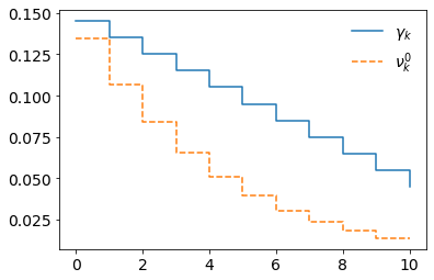
(a) Fair intensity function $(\gamma_{k})_{k\leq T-1}$ and trader’s intensity function $(\nu^{0}_{k})_{k\leq T-1}$ calibrated to the latter on the binaries at $t=0$.

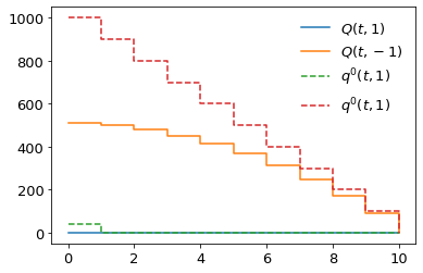
(b) Pricing functions of the callable range accrual in the fair valuation model, $Q(\cdot,\cdot)$, and in the trader’s model calibrated to the latter on the binaries at time 0, $q^{0}(\cdot,\cdot)$.

(c) Hedging ratios along the lower corridor $i=-1$ in the fair valuation model, $A_{0}(\ell)$, and in the trader’s model calibrated to the latter on binaries at time 0, $a_{0}(\ell)$.

(d) Hedging ratios along the upper corridor $i=+1$ in the fair valuation model, $B_{0}(\ell)$, and in the trader’s model calibrated to the latter on binaries at time 0, $b_{0}(\ell)$.

Figure 1: Jump intensity, pricing, and greeking functions.

Note that the pricing function $Q(\cdot,1)$ satisfies Assumption 5.2. Hence, based on Propositions 5.1-5.2 and their consequences detailed in Sections A.1-A.2, one has numerically access to an exhaustive description of the cases at hand, exact within machine precision (only involving discrete dynamic programming equations or exact formulas for path-dependent quantities, without Monte Carlo simulations). For sanity, we checked dynamically the validity of the martingale condition on the compensated $pnl$ processes of Propositions 5.1-5.2 in our numerics and these conditions were found to hold up to an accuracy of $10^{-16}$. We also checked that the conditional probabilities $\mathbb{Q}_{k}\left[\Omega_{\lambda}\right](\Omega_{l}),1\leq\lambda\leq T+1$ and $\mathbb{Q}_{k}\left[\Omega_{\lambda,\mu}\right](\Omega_{l,m}),(\lambda,\mu)\in\mathcal{I}$ as per Lemmas 5.6 and 5.9 were numerically non-negative and of sum one, for every respective index $1\leq l\leq T+1$ and $(l,m)\in\mathcal{I}$.

6.1 Bad Trader

For $\gamma(\cdot)$ as per (68), we find $\tau_{e}^{bad}\leq 2$. In fact, if ${\tau_{s}}=1$ or $2$, the bad trader calls back the option at that time. Otherwise, i.e. on $\{I_{0}=I_{1}=I_{2}=1\}$, the option has zero value in the trader’s model recalibrated at time 2, namely $q^{2}(2,1)=0$ (as computed exactly by dynamic programming), implying that he finds it optimal to call back the option at time 2, regardless of the model switch time ${\tau_{s}}>2$.

Hence the only relevant events are $\Omega_{1}$, $\Omega_{2}$ and $\Omega_{11}$ (on each $\Omega_{l}$, $l\geq 3$, everything happens as on $\Omega_{11}$). Figure 2 shows the bad trader’s $pnl$ on these events. We decompose the $pnl$ (center panel) in two terms (cf. the decomposition of $pnl_{k}$ in (55)): the cash flows ($\xi_{1}^{pnl}$) resulting from holding the option and its hedge plus the corresponding prices (top panel) and the term ($\xi_{2}^{pnl}$) accounting for calling the option at zero recovery (bottom panel). In the scenarios $\Omega_{1}$ and $\Omega_{2}$, where the asset is called due to the model switch, a profit (Figure 2, top panel) is more than compensated by calling the asset, highly valuable at that moment (Figure 2, bottom panel), resulting in an overall loss at the model switch time (Figure 2, center panel), in line with the corollary to the second Darwinian principle recalled in Section 1. Note that, in any time-${\tau_{s}}$ (hence, no longer calibrated) trader’s model and independently of the intensity $\nu^{{\tau_{s}}}$, as $i^{{\tau_{s}}}_{{\tau_{s}}}=I_{{\tau_{s}}}=-1$ is an absorbing state, the asset is worth $T-{\tau_{s}}$ and the hedge is worth $\sum_{k={\tau_{s}}+1}^{T}a_{0}(k)$. Hence the profit at the model switch time $\tau_{s}=1$ or $2$ made before calling the asset, as observed on the top panel of Figure 2, can be decomposed as follows (see Table 2):

$$\left(\mathcal{Q}_{\tau_{s}}+Q_{\tau_{s}}-(\mathcal{P}^{bad}_{\tau_{s}}+P^{bad}_{\tau_{s}})\right)-\left(\mathcal{Q}_{{\tau_{s}}-1}+q_{{\tau_{s}}-1}-(\mathcal{P}^{bad}_{{\tau_{s}}-1}+P^{bad}_{{\tau_{s}}-1}\right)=$$

$$\mathcal{Q}_{{\tau_{s}}}-\mathcal{Q}_{{\tau_{s}}-1}+(T-{\tau_{s}})-q^{{\tau_{s}}-1}({\tau_{s}}-1,1)-\big{(}\mathcal{P}^{bad}_{{\tau_{s}}}-\mathcal{P}^{bad}_{{\tau_{s}}-1}+\sum_{k={\tau_{s}}+1}^{T}a_{0}(k)-P^{bad}_{{\tau_{s}}-1}\big{)}$$

$$\;\;\;\;\;\;\;\;\;+Q({\tau_{s}},-1)-(T-{\tau_{s}})-\big{(}P^{bad}_{{\tau_{s}}}-\sum_{k={\tau_{s}}+1}^{T}a_{0}(k)\big{)},$$ (69)

where the last line corresponds to the change of valuation model at ${\tau_{s}}$, which is a loss as per Figure 1(b). An overall profit (made, at least, before calling the asset) means that this loss is more than compensated by a profit coming from the first line, coming from the static hedge not being perfect, especially at ${\tau_{s}}$ (from ${\tau_{s}}$ onward, the perfect hedge would be to short a digital option with payoff $\mathds{1}_{\{{I_{k}=-1}\}}$ for each $k>\tau_{s}$).

	$\Omega_{1}$	$\Omega_{2}$
$\mathcal{Q}_{{\tau_{s}}}-\mathcal{Q}_{{\tau_{s}}-1}+(T-{\tau_{s}})-q^{{\tau_{s}}-1}({\tau_{s}}-1,1)$
$-(\mathcal{P}^{bad}_{{\tau_{s}}}-\mathcal{P}^{bad}_{{\tau_{s}}-1}+\sum_{k={\tau_{s}}+1}^{T}a_{0}(k)-P^{bad}_{{\tau_{s}}-1})$	$335$	$391$
$Q({\tau_{s}},-1)-(T-{\tau_{s}})-\big{(}P^{bad}_{{\tau_{s}}}-\sum_{k={\tau_{s}}+1}^{T}a_{0}(k)\big{)}$	$-227$	$-196$

Table 2: The decomposition (69) on the events $\Omega_{1}$ and $\Omega_{2}$.

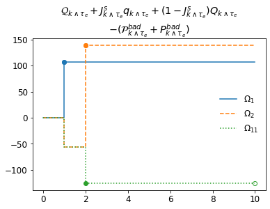
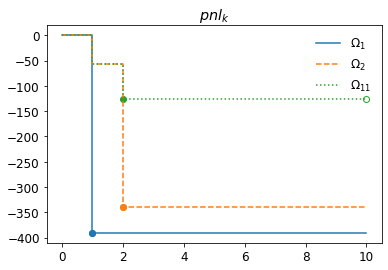
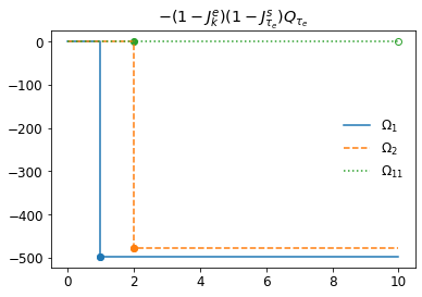
Figure 2: (center) bad trader’s $pnl$, (top) callable option cashflow and price minus its hedge cashflow and price, (bottom) term accounting for calling the product (at zero recovery).

Figure 3 shows the bad trader’s ${\rm HVA}$ process (top left panel) and its split into three contributions (cf. the decomposition of ${\rm HVA}_{k}$ in (55)): the misvaluation term $\xi^{hva}$ when the trader uses his own model instead of the fair valuation one (top right), the adjustment $\chi^{hva}_{1}+\chi^{hva}_{2}$ when the call occurs before the switch time (bottom left), and the compensating term $\chi^{hva}_{3}$ for the option cashflow and price (bottom right). We observe that the HVA on a callable claim (top left) can thus be several times greater than the price difference $q-Q$ (top right).

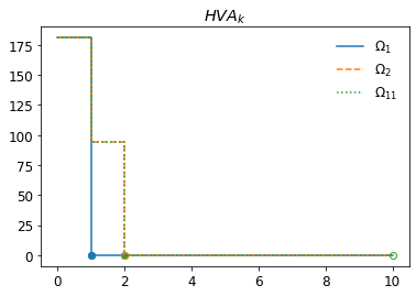
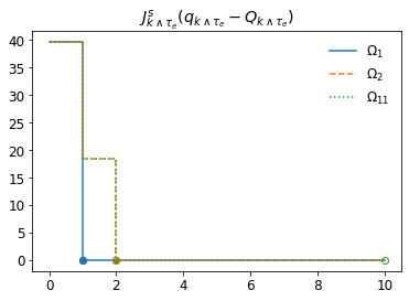
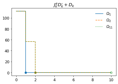
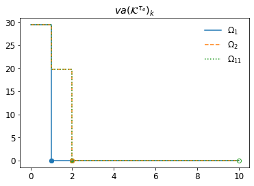
Figure 3: Bad trader’s ${\rm HVA}$ and its components.

Figure 4 displays the HVA compensated $pnl$ process of the bad trader. We notice that on the event $\Omega_{11}$, where there is no switch and the trader calls back the claim at time 2, the ${\rm HVA}$ depreciation gains cover the $pnl$ losses (the green curve is in the negative), in line with the second Darwinian principle of Section 1 detailed as Albanese, Bénézet, and Crépey (2022, Remark 2.5). On $\Omega_{1}$ and $\Omega_{2}$, the losses made at ${\tau_{s}}$ supersede the systematic profits made before ${\tau_{s}}$.

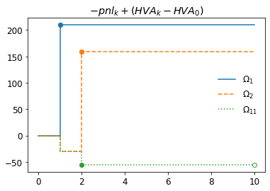
Figure 4: HVA-compensated loss-and-profits of the bad trader.

6.2 Not-So-Bad Trader

Regarding the not-so-bad trader, as $q^{2}(2,1)=0$, the option is called at $k=2$ if the model switch has not occurred before. Hence all the $\Omega_{l,m},\;3\leq l\leq 10,$ are equivalent to $\Omega_{11,11}$. As for $l\leq 2$, on $\Omega_{l,m}$, the not-so-bad trader always calls the option at time $m$, which is the first time beyond $l$ for which $Q(m,I_{m})=Q(m,1)=0$. Accordingly, we only report on the results corresponding to the events $\Omega_{l,m}$, for $l=1$ or $2$ and $m>l$, and $\Omega_{11,11}$.

Figure 5 displays the not-so-bad trader’s ${\rm HVA}$ and its split in valuation (Figures 5(c) and 5(d)) and early callability (Figure 5(b)) components. The corresponding process $D$ as per (67) vanishes, as $J^{s}_{{\tau_{e}}}Q_{{\tau_{e}}}=0$ under Assumption 5.2, while $J^{s}_{{\tau_{e}}}P^{nsb}_{\tau_{e}}=J^{s}_{{\tau_{e}}}P^{bad}_{\tau_{e}},$ by (20) (which holds likewise in the discrete setup). Hence what we can see on Figure 5(b) in fact reduces to $va(K^{\tau_{e}})_{k}$. The comparison with the the top left panel of Figure 3 shows that the not-so-bad trader’s ${\rm HVA}$ is much (almost twice) smaller than the one of the bad trader. But the HVA of the not-so-bad trader is still significantly greater than the price differences $J^{s}(q-Q)$ or $J^{s}(q-Q-(p-P))=J^{s}(q-Q-(P^{bad}-P^{nsb}))$ (compare Figures 5(c) and 5(d)), even if much less so than what we had in the case of the bad trader (cf. Figure 3 and comments).

Figures 6 and 7 display the not-so-bad trader’s $pnl$ and HVA compensated $pnl$ process. As opposed to what we saw in Figure 4 regarding the bad trader, on the event $\Omega_{11,11}$, where there is no switch and the trader calls back the claim according to the prescriptions of his wrong model, the ${\rm HVA}$ depreciation gains no longer cover the $pnl$ losses (the dotted curve is in the positive in Figure 7): the better practice of switching to the fair valuation model once the trader’s model no longer calibrates not only diminishes the HVA, but also avoids the wrong message that the HVA-compensated trader would make legit liquidity gains, while in expectation these systematic gains in fact only compensate future losses.

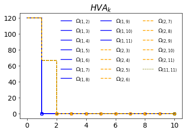
(a) Not-so-bad trader’s HVA

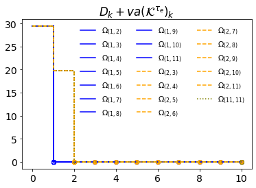
(b) Valuation adjustment of the option’s cashflow and price processes

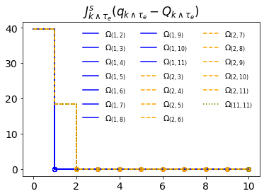
(c) Fair valuation of the portfolio and its cumulative dividend

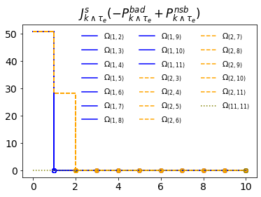
(d) Fair valuation of the hedge and its cumulative dividend

Figure 5: Not-so-bad trader’s ${\rm HVA}$ and its components.

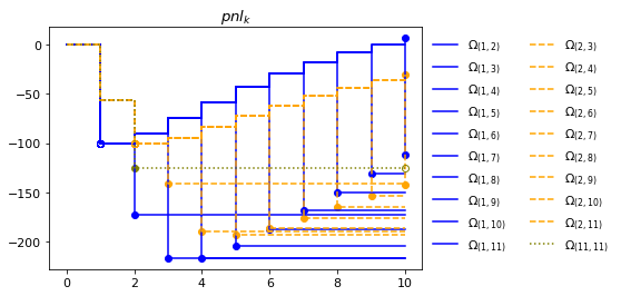
Figure 6: Not-so-bad trader’s $pnl$.

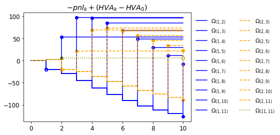
Figure 7: HVA-compensated loss-and-profits of the not-so-bad trader.

Figures 8 gathers on the same graphs the previous results in the event where the switch never happens, i.e. on $\Omega_{11}$ in the case of the bad trader and $\Omega_{11,11}$ in the case of the not-so-bad one. The corresponding paths of the $pnl$ appear to be identical (as they indeed are) in the top panel of Figure 8. As explained above, the ${\rm HVA}$ of the not-so-bad trader is smaller than the one of the bad one (middle panel); the HVA depreciation gains of the bad trader fakely more than compensate his raw $pnl$ losses, but this is not the case for the not-so-bad trader (top and bottom panels), who is thus incentivized to what would be the best (and only advisable) practice, namely only using the fair valuation model for all his purposes, also in line with (Albanese, Bénézet, and Crépey, 2022, Conclusion)).

Conclusion

Figures 9 and 10 show the economic capital processes of the two traders as per Propositions 5.1-5.2 (iii), resulting in the KVA₀ (for a hurdle rate $r$ of 10%) displayed in Table 3, along with the corresponding HVA₀. As expected, ${\rm HVA}^{nsb}_{0}\leq{\rm HVA}^{bad}_{0}$ and $\mathrm{KVA}^{nsb}_{0}\leq\mathrm{KVA}^{bad}_{0}$. In this simple example, the KVA is largely dominated by the HVA, by a factor $>5$, whereas the opposite was prevailing in the case of model risk on a European claim in Albanese, Bénézet, and Crépey (2022, Eqn. (3.10)). However, a common and salient conclusion is that, in all the considered examples (bad or not-so-bad trader dealing a callable claim here or bad trader dealing a European claim in the previous paper), the risk-adjusted HVA, ${\rm AVA}={\rm HVA}+\mathrm{KVA}$ (additional valuation adjustment for model risk), is much larger (even several times, in the case of the bad traders of this or the previous paper) than the price difference $q-Q$ (mainly due to an HVA effect in the present callable case, see Figures 3 and 5, and to a KVA effect in the previous paper). This provides quantitative arguments in favour of a reserve for model risk that should be much larger than the common practice of reserving $q-Q$ simply (cf. Albanese, Bénézet, and Crépey (2022, Remark 2.5)). We also reassert from Albanese, Crépey, and Iabichino (2021) that Darwinian model risk cannot be detected by standard market risk metrics such as value-at-risk, expected shortfall or stressed value-at-risk. Model risk derives from the cumulative effect of daily recalibrations and feeds into the first moment of returns (alpha leakages). The usual market risk metrics, instead, all focus on higher moments of return distributions at short-time horizons (such as one day). Model risk can only be seen by simulating the hedging behaviour of a bad model within a good model, recalibrating the bad model on-the-fly as done in the elementary cases of this paper or Albanese, Bénézet, and Crépey (2022) (in which the HVA can be computed effectively) or, at least, proceeding by state-space analysis as demonstrated in a realistic setup in Albanese, Crépey, and Iabichino (2021). Note that dynamic recalibration in a realistic simulation setup is not necessarily out-of-scope with the help of the emerging machine learning fast calibration techniques. However, again, the best practice would be that banks only rely on high-quality models, so that such computations are simply not necessary.

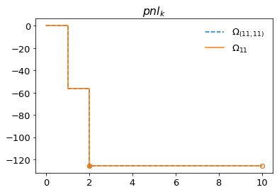
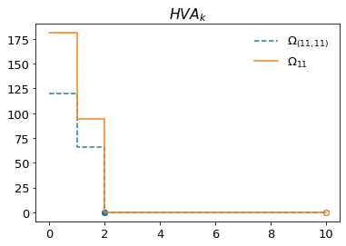
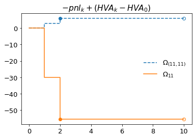
Figure 8: (top) $pnl$, (center) ${\rm HVA}$, and (bottom) ${\rm HVA}_{(0)}-pnl$ of the bad trader and the not-so-bad trader in the absence of model switch.

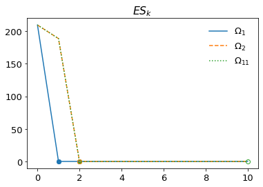
Figure 9: Worst trader’s expected shortfall

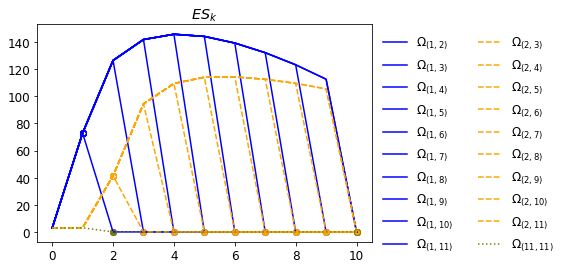
Figure 10: Not-so-bad trader’s expected shortfall

	${\rm HVA}_{0}$	$\mathrm{KVA}_{0}$
bad trader	$181$	$36$
not-so-bad trader	$120$	$10$

Table 3: ${\rm HVA}_{0}$ and $\mathrm{KVA}_{0}$ of the traders.

Appendix A Computational Details Regarding $P$

As opposed to $P^{bad}$, $P^{nsb}$ does not satisfy an obvious dynamic programming principle. What follows is used in our numerics.

A.1 Bad Trader

Note that, for $1\leq\lambda\leq T+1$ and $0\leq\kappa\leq\lambda\wedge T,$

$$\begin{aligned} &\mathds{1}_{\{{I_{\kappa}=-1}\}}(\Omega_{\lambda})=\mathbf{1}_{\kappa=\lambda}.\end{aligned}$$ (70)

Hence, by the first line in (50),

$$\begin{aligned} \mathcal{P}^{bad}_{\kappa}(\Omega_{\lambda})&=\sum_{\ell=1}^{\kappa}\big{(}{a}_{0}(\ell)\mathbf{1}_{\ell=\lambda}-{b}_{0}(\ell)\mathbf{1}_{\ell<\lambda}\big{)}.\end{aligned}$$ (71)

In addition, by the third line in (50) and (38), we have, for $\kappa\leq\lambda\wedge T,$

$$\begin{aligned} &P^{bad}_{\kappa}(\Omega_{\lambda})=\sum_{\ell=\kappa+1}\Big{(}a_{0}(\ell)P_{\kappa}(\ell)(\Omega_{\lambda})-b_{0}(\ell)\big{(}1-P_{\kappa}(\ell)(\Omega_{\lambda})\big{)}\Big{)}\mbox{ with}\\ &\;\;\;\;\;\;\;\;\;P_{\kappa}(\ell)(\Omega_{\lambda})=\mathbf{1}_{\kappa<\lambda}\frac{1-e^{-2h\sum_{\mu=k}^{\ell-1}\gamma_{\mu}}}{2}+\mathbf{1}_{\kappa=\lambda}\frac{1+e^{-2\sum_{\mu=k}^{\ell-1}\gamma_{\mu}}}{2}.\end{aligned}$$ (72)

In conclusion, for every $0\leq k\leq T$ and $1\leq\lambda\leq T+1$ so that $k\wedge{\tau_{e}}(\Omega_{\lambda})\leq\lambda\wedge T$, $\mathcal{P}^{bad}_{k\wedge{\tau_{e}}(\Omega_{\lambda})}(\Omega_{\lambda})$ and $P^{bad}_{k\wedge{\tau_{e}}(\Omega_{\lambda})}(\Omega_{\lambda})$ can be computed by (71) and (72) for $\kappa=k\wedge{\tau_{e}}(\Omega_{\lambda})$.

Also (cf. the second line in (38)),

$$\begin{aligned} &P^{bad}_{k}=P^{bad}(k,I_{k}),\,P^{bad}_{k\wedge{\tau_{e}}(\Omega_{\lambda})}(\Omega_{\lambda})=P^{bad}\big{(}k\wedge{\tau_{e}}(\Omega_{\lambda}),I_{k\wedge{\tau_{e}}(\Omega_{\lambda})}(\Omega_{\lambda})\big{)},\end{aligned}$$

where

$$\begin{aligned} &P^{bad}(T,\mp 1)=0\mbox{ and, for }0\leq k<T,\\ &P^{bad}(k,-1)=u_{k+1}\big{(}{a}_{0}(k+1)h+P^{bad}(k+1,-1)\big{)}+v_{k+1}\big{(}-{b}_{0}(k+1)h+P^{bad}(k+1,1)\big{)}\\ &\;\;\;\;\;\;\;\;\;=hu_{k+1}{a}_{0}(k+1)-hv_{k+1}{b}_{0}(k+1)+v_{k+1}P^{bad}(k+1,1)+u_{k+1}P^{bad}(k+1,-1),\\ &P^{bad}(k,1)=v_{k+1}\big{(}{a}_{0}(k+1)h+P^{bad}(k+1,-1)\big{)}+u_{k+1}\big{(}-{b}_{0}(k+1)h+P^{bad}(k+1,1)\big{)}\\ &\;\;\;\;\;\;\;\;\;=hv_{k+1}{a}_{0}(k+1)-hu_{k+1}{b}_{0}(k+1)+u_{k+1}P^{bad}(k+1,1)+v_{k+1}P^{bad}(k+1,-1).\end{aligned}$$ (73)

A.2 Not-So-Bad Trader

Lemma A.1.

For every $0\leq k\leq T$ and $(\lambda,\mu)\in\mathcal{I}$ such that $k\leq\mu$,

$$\begin{aligned} \mathds{1}_{\{{I_{k}=-1}\}}(\Omega_{{\lambda,\mu}})=\mathbf{1}_{\lambda\leq k<\mu}.\end{aligned}$$ (74)

Proof.  We compute

$$\begin{aligned} &\mathds{1}_{\{{I_{k}=-1}\}}(\Omega_{T+1,T+1})=0,\\ &\mathds{1}_{\{{I_{k}=-1}\}}(\Omega_{\lambda,T+1})=\mathbf{1}_{k\geq\lambda},\,\lambda\leq T,\\ &\mathds{1}_{\{{I_{k}=-1}\}}(\Omega_{\lambda,\mu})=\mathbf{1}_{\lambda\leq k<\mu},\,k,\lambda\leq\mu\leq T,\end{aligned}$$

which we can summarize as (74) that is valid for every $0\leq k\leq T$ and $(\lambda,\mu)\in\mathcal{I}$ such that $k\leq\mu$.  

Given the specification (58) of $\mathcal{P}^{nsb}_{k}$, we have

$$\begin{aligned} &\mathcal{P}^{nsb}_{k}(\Omega_{\lambda,\mu})=\sum_{\ell=1}^{k\wedge{\tau_{s}}(\Omega_{\lambda,\mu})}\left({a}_{0}(\ell)\mathds{1}_{\{{I_{\ell}=-1}\}}(\Omega_{\lambda,\mu}){-{b}_{0}(\ell)\mathds{1}_{\{{I_{\ell}=1}\}}}(\Omega_{\lambda,\mu})\right)\\ &+(1-J^{s}_{k}(\Omega_{\lambda,\mu}))J^{s}_{{\tau_{e}}(\Omega_{\lambda,\mu})}(\Omega_{\lambda,\mu})\\ &\;\;\;\;\;\;\;\;\;\sum_{\ell={\tau_{s}}(\Omega_{\lambda,\mu})}^{k}\left({a}_{0}(\ell)\mathds{1}_{\{{I_{\ell}=-1}\}}(\Omega_{\lambda,\mu}){-{b}_{0}(\ell)\mathds{1}_{\{{I_{\ell}=1}\}}}\right)(\Omega_{\lambda,\mu})\\ &+(1-J^{s}_{k}(\Omega_{\lambda,\mu}))(1-J^{s}_{{\tau_{e}}(\Omega_{\lambda,\mu})}(\Omega_{\lambda,\mu}))\\ &\;\;\;\;\;\;\;\;\;\sum_{\ell={\tau_{s}}(\Omega_{\lambda,\mu})}^{k}\left({A}_{{\tau_{s}}(\Omega_{\lambda,\mu})}(\ell)(\Omega_{\lambda,\mu})\mathds{1}_{\{{I_{\ell}=-1}\}}(\Omega_{\lambda,\mu}){-{B}_{{\tau_{s}}(\Omega_{\lambda,\mu})}(\ell)(\Omega_{\lambda,\mu})\mathds{1}_{\{{I_{\ell}=1}\}}(\Omega_{\lambda,\mu})}\right),\end{aligned}$$ (75)

where the $\mathds{1}_{\{{I_{\ell}=\mp 1}\}}(\Omega_{\lambda,\mu})$ are given by (74), whereas (42) and (66) yield on $k={\tau_{s}}(\Omega_{\lambda,\mu})$:

$$\begin{aligned} &{A}_{k}(\ell)(\Omega_{\lambda,\mu})=\frac{\sum_{(\lambda^{\prime},\mu^{\prime})\in\mathcal{I}}\mathds{1}_{\{{I_{\ell}=-1}\}}(\Omega_{\lambda^{\prime},\mu^{\prime}})\mathds{1}_{\{{t_{\ell}\leq\tau^{k}(\Omega_{\lambda^{\prime},\mu^{\prime}})}\}}\mathbb{Q}_{k}\left[\Omega_{\lambda^{\prime},\mu^{\prime}}\right](\Omega_{\lambda,\mu})}{P_{k}(\ell)(\Omega_{\lambda,\mu})}&\\ &=\frac{\sum_{(\lambda^{\prime},\mu^{\prime})\in\mathcal{I}}\mathbf{1}_{\lambda^{\prime}\leq\ell<\mu^{\prime}}\mathbf{1}_{\ell\leq\mu^{\prime}}\mathbb{Q}_{k}\left[\Omega_{\lambda^{\prime},\mu^{\prime}}\right](\Omega_{\lambda,\mu})}{P_{k}(\ell)(\Omega_{\lambda,\mu})}=\frac{\sum_{(\lambda^{\prime},\mu^{\prime})\in\mathcal{I}}\mathbf{1}_{\lambda^{\prime}\leq\ell<\mu^{\prime}}\mathbb{Q}_{k}\left[\Omega_{\lambda^{\prime},\mu^{\prime}}\right](\Omega_{\lambda,\mu})}{P_{k}(\ell)(\Omega_{\lambda,\mu})},\end{aligned}$$ (76)

and we likewise have by (42):

$$\begin{aligned} {B}_{k}(\ell)(\Omega_{\lambda,\mu})=\frac{\sum_{(\lambda^{\prime},\mu^{\prime})\in\mathcal{I}}(1-\mathbf{1}_{\lambda^{\prime}\leq\ell<\mu^{\prime}})\mathbf{1}_{\ell\leq\mu^{\prime}}\mathbb{Q}_{k}\left[\Omega_{\lambda^{\prime},\mu^{\prime}}\right](\Omega_{\lambda,\mu})}{1-P_{k}(\ell)(\Omega_{\lambda,\mu})}.\end{aligned}$$ (77)

Besides, by the second identity in (60), we have, for every $(\lambda,\mu)\in\mathcal{I}$,

$$\begin{aligned} &P^{nsb}_{{\tau_{e}}(\Omega_{{\lambda,\mu}})}(\Omega_{{\lambda,\mu}})=J^{s}_{{\tau_{e}}(\Omega_{\lambda,\mu})}\\ &\;\;\;\;\;\;\;\;\;\sum_{\ell={{\tau_{e}}(\Omega_{\lambda,\mu})}+1}\Big{(}a_{0}(\ell)P_{{\tau_{e}}(\Omega_{\lambda,\mu})}(\ell)(\Omega_{\lambda,\mu})-b_{0}(\ell)\big{(}1-P_{{\tau_{e}}(\Omega_{\lambda,\mu})}(\ell)(\Omega_{\lambda,\mu})\big{)}\Big{)}\\ &+(1-J^{s}_{{\tau_{e}}(\Omega_{\lambda,\mu})})\\ &\;\;\;\;\;\;\;\;\;\sum_{\ell={{\tau_{e}}(\Omega_{\lambda,\mu})}+1}\Big{(}{A}_{{\tau_{s}}(\Omega_{\lambda,\mu})}(\ell)(\Omega_{\lambda,\mu})P_{{\tau_{e}}(\Omega_{\lambda,\mu})}(\ell)(\Omega_{\lambda,\mu})\\ &\;\;\;\;\;\;\;\;\;\;\;\;\;\;\;\;\;\;-{B}_{{\tau_{s}}(\Omega_{\lambda,\mu})}(\ell)(\Omega_{\lambda,\mu})\big{(}1-P_{{\tau_{e}}(\Omega_{\lambda,\mu})}(\ell)(\Omega_{\lambda,\mu})\big{)}\Big{)},\end{aligned}$$ (78)

where for $\kappa\leq\mu\wedge T$ (note that ${\tau_{e}}(\Omega_{\lambda,\mu})\leq\mu\wedge T$)

$$\begin{aligned} &P_{\kappa}(\ell)(\Omega_{{\lambda,\mu}})\\ &=\mathds{1}_{\{{I_{\kappa}=-1}\}}(\Omega_{{\lambda,\mu}})\frac{1+e^{-2\sum_{i=\kappa}^{\ell-1}\gamma_{i}}}{2}+\mathds{1}_{\{{I_{\kappa}=1}\}}(\Omega_{{\lambda,\mu}})\frac{1-e^{-2h\sum_{i=\kappa}^{\ell-1}\gamma_{i}}}{2}\\ &=\mathds{1}_{\{{I_{\kappa}=-1}\}}(\Omega_{{\lambda,\mu}})\mathbf{1}_{\kappa={\lambda,\mu}}\frac{1+e^{-2\sum_{i=\kappa}^{\ell-1}\gamma_{i}}}{2}+\mathds{1}_{\{{I_{\kappa}=1}\}}(\Omega_{{\lambda,\mu}})\mathbf{1}_{\kappa<{\lambda,\mu}}\frac{1-e^{-2h\sum_{i=\kappa}^{\ell-1}\gamma_{i}}}{2},\end{aligned}$$ (79)

in which the $\mathds{1}_{\{{I_{\kappa}=\mp 1}\}}(\Omega_{{\lambda,\mu}})$ are deduced from (74). Hence, for every $k\leq{\tau_{e}}$ and $(l,m)\in\mathcal{I}$, (59) yields

$$\begin{aligned} &P^{nsb}_{k}(\Omega_{l,m})=\mathbb{E}_{k}\left[\mathcal{P}^{nsb}_{{\tau_{e}}}-\mathcal{P}^{nsb}_{k}+P^{nsb}_{{\tau_{e}}}\right](\Omega_{l,m})=\\ &\;\;\;\;\;\;\;\;\;\sum_{(\lambda,\mu)\in\mathcal{I}}\big{(}\mathcal{P}^{nsb}_{{\tau_{e}}(\Omega_{\lambda,\mu})}(\Omega_{\lambda,\mu})-\mathcal{P}^{nsb}_{k}(\Omega_{\lambda,\mu})+P^{nsb}_{{\tau_{e}}(\Omega_{\lambda,\mu})}(\Omega_{\lambda,\mu})\big{)}\mathbb{Q}_{k}\left[\Omega_{\lambda,\mu}\right](\Omega_{l,m}),\end{aligned}$$ (80)

by (66), where all terms can be computed by (60) and (74)–(79). Finally, for every $0\leq k\leq T$ and $(\lambda,\mu)\in\mathcal{I}$, we have

$$\begin{aligned} &P^{nsb}_{k\wedge{\tau_{e}}}(\Omega_{\lambda,\mu})=P^{nsb}_{k\wedge{\tau_{e}}(\Omega_{\lambda,\mu})}(\Omega_{\lambda,\mu}).\end{aligned}$$ (81)

References

- Acerbi and Tasche (2002) Acerbi, C. and D. Tasche (2002). On the coherence of expected shortfall. Journal of Banking & Finance 26(7), 1487–1503.
- Albanese et al. (2017) Albanese, C., S. Caenazzo, and S. Crépey (2017). Credit, funding, margin, and capital valuation adjustments for bilateral portfolios. Probability, Uncertainty and Quantitative Risk 2(7), 26 pages.
- Albanese et al. (2022) Albanese, C., C. Bénézet, and S. Crépey (2022). Hedging valuation adjustment and model risk. arXiv:2205.11834.
- Albanese et al. (2021) Albanese, C., S. Crépey, and S. Iabichino (2021). A Darwinian theory of model risk. Risk Magazine, July pages 72–77.
- Artzner et al. (2020) Artzner, P., K.-T. Eisele, and T. Schmidt (2020). No arbitrage in insurance and the QP-rule. arXiv:2005.11022.
- Burnett (2021) Burnett, B. (2021). Hedging value adjustment: Fact and friction. Risk Magazine, February 1–6.
- Burnett and Williams (2021) Burnett, B. and I. Williams (2021). The cost of hedging XVA. Risk Magazine, April.
- Karoui et al. (1998) Karoui, N. E., M. Jeanblanc-picqué, and S. E. Shreve (1998). Robustness of the black and scholes formula. Mathematical Finance 8(2), 93–126.