$\mathsf{PrivGraph}$: Differentially Private Graph Data Publication
by Exploiting Community Information

Abstract

Graph data is used in a wide range of applications, while analyzing graph data without protection is prone to privacy breach risks. To mitigate the privacy risks, we resort to the standard technique of differential privacy to publish a synthetic graph. However, existing differentially private graph synthesis approaches either introduce excessive noise by directly perturbing the adjacency matrix, or suffer significant information loss during the graph encoding process. In this paper, we propose an effective graph synthesis algorithm $\mathsf{PrivGraph}$ by exploiting the community information. Concretely, $\mathsf{PrivGraph}$ differentially privately partitions the private graph into communities, extracts intra-community and inter-community information, and reconstructs the graph from the extracted graph information. We validate the effectiveness of $\mathsf{PrivGraph}$ on six real-world graph datasets and seven commonly used graph metrics.

1 Introduction

Many real-world systems can be represented by graphs, such as social networks [37], email networks [38], voting networks [44], etc., and analyzing these graph data is beneficial in a wide range of applications [56]. For instance, Facebook analyzes social networks and makes friend recommendations based on the connections (edges) between various users (nodes) [29]. Due to the sensitive nature of the graph data, it cannot be directly analyzed without protection. A classical approach to analyzing the graph data while preserving privacy is anonymization, which removes the identification information of the nodes [64, 9]. However, previous studies have shown that the anonymized graphs can be easily deanonymized by the attackers when they have some auxiliary information [27, 48].

To overcome the drawback of the anonymization techniques, differential privacy (DP) [15, 13, 75, 61], a golden standard in the privacy community, has been applied to protect the privacy of graph data [55, 68]. The core idea of DP is to guarantee that a single node/edge has a limited impact on the final output. Most of the previous studies on differentially private graph analysis focus on designing tailored algorithms for specific graph analysis tasks, such as degree distribution [24], subgraph counts [58], and community discovery [28]. Our paper, on the other hand, focuses on a more general paradigm, which publishes a synthetic graph that is semantically similar to the original graph while satisfying DP. This paradigm is superior to the tailored algorithms in the sense that it enables arbitrary downstream graph data analysis tasks.

Existing Solutions. There are multiple existing studies focusing on publishing a synthetic graph under DP guarantee. In [45], Nguyen et al. proposed the Top-m Filter ($\mathsf{TmF}$) method that directly perturbs the adjacency matrix of the original graph. $\mathsf{TmF}$ adds Laplace noise to each cell of the adjacency matrix and selects the top-$m$ cells from the noisy matrix as edges for the synthetic graph, where $m$ is the total number of edges in the original graph. Note that directly perturbing the adjacency matrix introduces excessive noise; thus $\mathsf{TmF}$ can only restore a few true edges when the privacy budget is small. Chen et al. [6] designed the density-based exploration and reconstruction ($\mathsf{DER}$) method to perturb and reconstruct the adjacency matrix. $\mathsf{DER}$ relabels the nodes to make edges concentrate on specific areas of the adjacency matrix, and then leverages a quadtree to calculate the density of the adjacency matrix. To satisfy DP, the synthetic graph is reconstructed from the perturbed density. However, since the perturbation noise oftentimes overwhelms the true densities of the sparse areas, it is difficult for $\mathsf{DER}$ to maintain the structure of the original graph, and the computational complexity of constructing a quadtree is large. Different from $\mathsf{TmF}$ and $\mathsf{DER}$ that directly perturb the adjacency matrix of the original graph, $\mathsf{PrivHRG}$ encodes the graph into a hierarchical random graph (HRG) [11] under DP, which reduces the strength of the noise. However, $\mathsf{PrivHRG}$ needs a significant amount of time to build the HRG and suffers graph structure distortion. Qin et al. [49] proposed to divide the nodes into multiple groups using $k$-means clustering. However, the clustering accuracy under noise perturbation is usually low, which affects the accuracy of graph reconstruction.

Our Proposal. Existing methods either introduce excessive noise by directly perturbing the adjacency matrix, or suffer substantial information loss in the process of encoding the graph data. In this paper, we propose $\mathsf{PrivGraph}$ that exploits community information of the graph data to strike the trade-off between the perturbation noise and information loss.

To avoid the large perturbation caused by directly adding noise to each cell of the adjacency matrix, $\mathsf{PrivGraph}$ leverages a community division mechanism to group all nodes into multiple communities and add noise to the communities instead of nodes. However, existing community detection algorithms do not satisfy DP. Therefore, we design a two-step division mechanism under DP guarantee, i.e., community initialization and community adjustment. $\mathsf{PrivGraph}$ generates an initial community partition in community initialization and further tunes the nodes division in community adjustment. The community aggregates more information than each node, resulting in higher robustness to noise perturbation.

Based on the intuition that edges in a community are denser and edges between communities are sparser, we design two mechanisms to extract, perturb and reconstruct the edges of intra-community and inter-community separately, which preserve the structure information and suppress the noise simultaneously. Furthermore, we propose a post-processing procedure to maintain data fidelity.

Evaluation. We conduct experiments on six real-world graph datasets to illustrate the superiority of $\mathsf{PrivGraph}$. The experimental results show that $\mathsf{PrivGraph}$ outperforms the state-of-the-art methods for most of the metrics. For instance, when the privacy budget is 1, for the modularity metric, $\mathsf{PrivGraph}$ achieves 51.3% lower relative error than that of $\mathsf{PrivHRG}$ on the Facebook dataset. We also compare $\mathsf{PrivGraph}$ with tailored private methods optimized for specific graph analysis tasks. Then, we conduct an ablation study on the hyper-parameters of $\mathsf{PrivGraph}$ and provide guidelines to select them. We further illustrate the effectiveness of $\mathsf{PrivGraph}$ on a real-world application, i.e., influence maximization, which aims to find a small subset of nodes (seed nodes) in a graph that could maximize influence spread. We observe that the seed nodes obtained using $\mathsf{PrivGraph}$ achieves up to 58.6% higher influence spread than that of $\mathsf{DER}$ on the Facebook dataset.

Contributions. In summary, the main contributions of this paper are three-fold:

• We take a deep look at existing solutions on differentially private graph synthesis, and identify their major drawbacks.

• We propose a practical method $\mathsf{PrivGraph}$ to generate a synthetic graph under DP. The general idea is to group the nodes in the graph by community information to avoid introducing excessive noise, and adopt different reconstruction approaches based on the characteristics of intra-community and inter-community to retain the graph structure.

• We conduct extensive experiments and a real-world case study on multiple datasets and metrics to illustrate the effectiveness of $\mathsf{PrivGraph}$. $\mathsf{PrivGraph}$ is open-sourced at https://github.com/Privacy-Graph/PrivGraph.

2 Preliminaries

2.1 Differential Privacy

Differential Privacy (DP) [15] was originated for the data privacy-protection scenarios, where a trusted data curator collects data from individual users, perturbs the aggregated results, and then publishes it. Intuitively, DP guarantees that any single sample from the dataset has only a limited impact on the output. Formally, we can define DP as follows:

Definition 1 ($\varepsilon$-Differential Privacy).

An algorithm $\mathcal{A}$ satisfies $\varepsilon$-differential privacy ($\varepsilon$-DP), where $\varepsilon>0$, if and only if for any two neighboring datasets $D$ and $D^{\prime}$, we have

$$\forall T\subseteq Range(\mathcal{A}):\mathsf{Pr}\left[\mathcal{A}(D)\in T\right]\leq e^{\varepsilon}\mathsf{Pr}\left[\mathcal{A}(D^{\prime})\in T\right]$$

where Range $(\mathcal{A})$ denotes the set of all possible outputs of the algorithm $\mathcal{A}$.

We consider two datasets $D$ and $D^{\prime}$ to be neighbors, denoted as $D\simeq D^{\prime}$, if and only if $D=D^{\prime}+r$ or $D^{\prime}=D+r$, where $D+r$ stands for the dataset resulted from adding the record $r$ to the dataset $D$.

Laplace Mechanism. Laplace mechanism (LM) satisfies the DP requirements by adding random Laplace noise to the aggregated results. The magnitude of the noise depends on ${GS}_{f}$, i.e., global sensitivity,

$${GS}_{f}=\max_{D\simeq D^{\prime}}{\parallel f(D)-f(D^{\prime})\parallel}_{1},$$

where $f$ represents the aggregation function and $D$ (or $D^{\prime}$) is the users’ data. When $f$ outputs a scalar, the Laplace mechanism $\mathcal{A}$ is given below:

$$\mathcal{A}_{f}(D)=f(D)+\mathcal{L}\left(\frac{{GS}_{f}}{\varepsilon}\right),$$

where $\mathcal{L}(\beta)$ stands for a random variable sampled from the Laplace distribution $\mathsf{Pr}\left[\mathcal{L}(\beta)=x\right]=\frac{1}{2\beta}e^{-\left|x\right|/\beta}$. When $f$ outputs a vector, $\mathcal{A}$ adds independent samples of $\mathcal{L}(\beta)$ to each element of the vector.

Exponential Mechanism. Laplace mechanism (LM) applies to the scenario where the output of $f$ is a real value, while the output of Exponential Mechanism (EM) [43] is an item from a finite set. EM samples more accurate answers with higher probabilities based on an exponential distribution. It takes the data $v$ as input and samples a possible output $o$ from the set $\mathcal{O}$ according to a quality function $q$. The approach requires to design a quality function $q$ which takes as input the data $v$, a possible output $o$, and outputs a quality score. The global sensitivity of the quality function is defined as

$${GS}_{q}=\max_{o}\max_{v\simeq v^{\prime}}\left|q(v,o)-q(v^{\prime},o)\right|.$$

$\mathcal{A}$ satisfies $\varepsilon$-differential privacy under the following equation.

$$\mathsf{Pr}\left[\mathcal{A}_{q}(v)=o\right]=\frac{{\rm exp}\left(\frac{\varepsilon}{2{GS}_{q}}q\left(v,o\right)\right)}{{\textstyle\sum\limits_{o^{\prime}\in\mathcal{O}}}{\rm exp}\left(\frac{\varepsilon}{2{GS}_{q}}q(v,o^{\prime})\right)}$$

Composition Properties of DP. The following composition properties of DP are commonly used for building complex differentially private algorithms from simpler subroutines.

• Sequential Composition. Combining multiple subroutines that satisfy differential privacy for $\{\varepsilon_{1},\cdots,\varepsilon_{k}\}$ results in a mechanism satisfying $\varepsilon$-differential privacy for $\varepsilon={\sum_{i}\varepsilon_{i}}$.

• Parallel Composition. Given $k$ algorithms working on disjoint subsets, each satisfying DP for $\{\varepsilon_{1},\cdots,\varepsilon_{k}\}$, the result satisfies $\varepsilon$-differential privacy for $\varepsilon=\max\{\varepsilon_{i}\}$.

• Post-processing. Given an $\varepsilon$-DP algorithm $\mathcal{A}$, releasing $g(\mathcal{A}(D))$ for any $g$ still satisfies $\varepsilon$-DP, i.e., post-processing an output of a differential private algorithm does not incur additional loss of privacy.

2.2 Differentially Private Graph Analysis

The edges of a graph may contain very sensitive information [27], such as social contacts, personal opinions, and private communication records [68, 6]. Edge-DP [24] provides rigorous theoretical guarantees to protect the privacy of these connections by limiting the impact of any edges in the graph on the output. As a result, it offers meaningful privacy protection in many applications [6, 45, 68].

More specifically, given a graph $G=(V,E)$, an edge neighboring graph $G^{\prime}=(V^{\prime},E^{\prime})$ can be obtained by adding (or removing) an edge, where $V$ ($V^{\prime}$) is the set of nodes and $E$ ($E^{\prime}$) is the set of edges. From [24], the system difference $a\oplus b$ is the sets of elements in either set $a$ or set $b$, but not in both, i.e., $a\oplus b=(a\cup b)\setminus(a\cap b)$. Hence, the definitions of edge neighboring graph and $\varepsilon$-edge DP are as follows.

Definition 2 (Edge neighboring graph).

Given a graph $G=(V,E)$, a graph $G^{\prime}=(V^{\prime},E^{\prime})$ is an edge neighboring graph of $G$ if and only if $\left|V\oplus V^{\prime}\right|+\left|E\oplus E^{\prime}\right|=1$.

Definition 3 ($\varepsilon$-edge differential privacy).

An algorithm $\mathcal{A}$ satisfies $\varepsilon$-edge differential privacy ($\varepsilon$-edge DP), where $\varepsilon>0$. If and only if for any two edge neighboring graphs G and $G^{\prime}$,

$$\forall T\subseteq Range(\mathcal{A}):\mathsf{Pr}\left[\mathcal{A}(G)\in T\right]\leq e^{\varepsilon}\mathsf{Pr}\left[\mathcal{A}(G^{\prime})\in T\right],$$

where $Range(\mathcal{A})$ denotes the set of all possible outputs of $\mathcal{A}$.

Discussion. Edge-DP guarantees that any edges in the graph have limited impacts on the final output, instead of deleting specific edges from the graph. As such, the attacker cannot infer the existence of any edges by observing the final output. The attacker can reconstruct the graph relying on auxiliary information such as some users are from the same class, but this is orthogonal to the privacy guarantee provided by DP. If the attacker has such auxiliary information, they can reconstruct these edges regardless of whether they are published.

Edge-DP is well-suited for scenarios where the edges are independent of each other, such as email communication records. However, in cases where the edges in a graph are correlated and can be deduced from one another, such as in a friendship graph, edge-DP’s guarantees may be insufficient while $k$-edge DP [24] can still provide meaningful privacy protection. In $k$-edge DP, graph $G$ and $G^{\prime}$ are neighbors if $\left|V\oplus V^{\prime}\right|+\left|E\oplus E^{\prime}\right|\leq k$.

The mechanism satisfying the formal definition of edge-DP also satisfies the requirements for $k$-edge DP. However, it’s important to note that achieving the same level of quality in published results using $k$-edge DP will require $k$ times more privacy budget than using edge-DP. For example, $\mathcal{A}$ satisfies $\varepsilon$-edge DP for $k=1$ and $\varepsilon=1$, it also satisfies $k$-edge $\varepsilon$-DP for $k=10$ and $\varepsilon=10$.

2.3 Community Detection

Community detection is an effective method for discovering densely connected subnetworks in graph data. It has a wide range of practical applications. For instance, in social networks, community detection helps identify a group of users with similar interests. A series of classical community detection algorithms have been proposed [3, 53, 4].

Louvain. The Louvain [3] method is adopted frequently due to its computing efficiency and outstanding grouping effect. The optimization goal of the Louvain method is to maximize the modularity [22], which measures the quality of the community division. The definition of modularity is as follows.

$$\small{Q}=\sum_{C}\left[\frac{\sum_{in}}{2m}-\left(\frac{{\sum_{tot}}}{2m}\right)^{2}\right],$$ (1)

where $\sum_{in}$ is the sum of the weights of the edges inside the community $C$, $\sum_{tot}$ stands for the sum of the weights of the edges incident nodes in $C$, and $m$ represents the sum of the weights of all edges.

At the beginning, Louvain randomly initializes each node as a single-node community. Then, Louvain iterates the following two processes until the modularity converges. Firstly, for each node in the graph, Louvain finds the largest gain in modularity by assigning the node to its neighbors’ community. If there exists no positive gain, the node will stay in the original community. This phase stops when a local maximum of the modularity is obtained, i.e. no individual move can enlarge the modularity. Then, Louvain merges the nodes in a community into a super-node and updates the weights of super-nodes. The weights between super-nodes are determined by the sum of the edges’ weights between two communities. The inner weight of a super-node is the sum of the edges’ weights inside the community. The purpose of the first step is to achieve modularity optimization and the second step is to complete the aggregation of nodes in the same community. According to [18], the modularity-based approaches might lose the small communities during the modularity optimization process. However, the information extraction and graph reconstruction processes of $\mathsf{PrivGraph}$ can recover these small communities. In the information extraction process, $\mathsf{PrivGraph}$ leverages a degree sequence to encode the edges in a community, where the dense connections of small communities are still preserved. Then, $\mathsf{PrivGraph}$ decodes the degree sequence and rebuilds the small communities. The above analysis are further supported by the experimental results in Section 5.4.

In addition, time-scale is a hyper-parameter to adjust the resolution of community detection [35]. By integrating time-scale $t$, modularity optimization can reveal the community structures at different resolutions, and the objective function is updated as follows.

$${Q^{*}}=\sum_{C}\left[\frac{\sum_{in}}{2m}t-\left(\frac{{\sum_{tot}}}{2m}\right)^{2}\right],$$

where $t$ is the resolution parameter, and the meanings of other parameters are the same as those in Equation 1. When $t=0$, each node occupies one community. When $t=1$, the optimization goal is consistent with traditional modularity optimization. When $t$ increases, the number of communities usually decreases. We further analyze the impact of different time-scale settings in Section E.3.

Discussion. Intuitively, clustering can partition nodes into groups like Louvain. However, compared to Louvain, it introduces new hyperparameters, such as the node’s feature, the distance metric, and the group size, which make clustering more challenging to tune under the noise perturbation.

3 Problem Definition and Existing Solutions

3.1 Problem Definition

Threat Model. With full access to the published graph, the adversary’s goal is to infer whether an edge exists in the original graph. For example, given a synthetic email communication network, the adversary aims to determine if there is an email connection between any two users.

In this paper, we consider an undirected and unweighted graph $G=(V,E)$, where $V$ is the set of nodes and $E$ is the set of edges. We are interested in the following problem: Given a graph $G$, how to generate a synthetic graph $G_{s}$ that shares similar graph properties with the original graph $G$ while satisfying edge-DP. The synthetic graph $G_{s}$ can be used for any downstream graph analysis tasks without privacy loss due to the post-processing property of DP. We summarize the frequently used mathematical notations in Table 1.

Following previous studies [6, 68, 45], we measure the similarity between $G_{s}$ and $G$ from five different aspects: Community discovery, node information, degree distribution, path condition, and topology structure. Concretely, the community discovery aims to detect the communities and reveal the structure of the graph, the node information reflects the neighboring information of each node, the degree distribution reveals the overall connection density of the graph, the path condition reflects the connectivity of the graph, and the topology structure illustrates the level of node aggregation.

Table 1: Summary of mathematical notations.

Notation	Description
$G$	Graph
$\varepsilon$	Privacy budget
$N$	The number of nodes per initial community
${m_{1}}$	The number of initial communities
${m_{2}}$	The number of final communities
$w$	The weight of the weighted graph
$\mathbb{C}$	The set of community partitions
$C$	The community composed of nodes
$d$	Degree sequence
$v$	Edge vector
$s$	Subgraph

3.2 Existing Solutions

TmF [45]. It first perturbs the adjacency matrix of the original graph by adding Laplace noise to each cell. Then, $\mathsf{TmF}$ chooses the top-$m$ noisy cells as edges in the perturbed adjacency matrix, where $m$ is obtained by adding Laplace noise to the true number of edges to satisfy DP. However, perturbing the whole cells in the adjacency matrix introduces excessive noise. Most true edges cannot be retained from the top-$m$ noisy cells, especially when $\varepsilon$ is small.

Although the computational cost of $\mathsf{TmF}$ is small, i.e., running in linear computational complexity, it faces several limitations: 1) $\mathsf{TmF}$ cannot capture the structure of the graph accurately since the selection of edges is random. 2) With a fixed privacy budget, the utility of the synthetic graph will decrease as the number of nodes increases.

DER [6]. Similar to TmF [45], $\mathsf{DER}$ also processes the adjacency matrix of the original graph. $\mathsf{DER}$ mainly consists of three steps: Node relabeling, dense region exploration, and edge reconstruction. $\mathsf{DER}$ first makes the edges in the adjacency matrix clustered together in the node relabeling step. Then, $\mathsf{DER}$ divides the adjacency matrix into multiple blocks and estimates the density by a noisy quadtree. Finally, $\mathsf{DER}$ reconstructs the edges in each block by exponential mechanism.

$\mathsf{DER}$ has two main drawbacks: 1) The time- and space-complexity of $\mathsf{DER}$ are quadratic, hindering its applications for large scale graphs. 2) The original graph structure is hard to maintain in dense region exploration.

PrivHRG [68]. $\mathsf{PrivHRG}$ captures the graph structure by using a statistical HRG [11], which aims to suppress the noise strength. The likelihood of an HRG for a graph $G$ shows how plausible the HRG is to represent $G$. An HRG with a higher likelihood can represent the structure of the original graph better than those with lower likelihoods.

The method first maps all nodes of a graph into a hierarchical structure and records connection probabilities between any pair of nodes in the graph. Then, $\mathsf{PrivHRG}$ uses the Markov chain Monte Carlo (MCMC) method to obtain an HRG with high likelihood while satisfying edge-DP. Finally, the edges are reconstructed based on the perturbed probabilities.

However, $\mathsf{PrivHRG}$ faces two limitations in practice: 1) It is time- and space-consuming to sample a high-quality HRG, especially when the amount of nodes is large. 2) The partial information of the graph is lost when constructing an HRG, which decays the accuracy of $\mathsf{PrivHRG}$.

LDPGen [49]. $\mathsf{LDPGen}$ is initially designed to generate a synthetic graph under local differential privacy (LDP). $\mathsf{LDPGen}$ first divides all nodes into two groups randomly. Then, $\mathsf{LDPGen}$ modifies the partition of the nodes by $k$-means clustering according to the number of connected edges from the nodes to each group, where the number of clusters is a pre-defined value. Finally, the connected edges are reconstructed based on the grouping and connected information. The idea of $\mathsf{LDPGen}$ can be ported to the DP setting. The main modification is in the $k$-means clustering, where the number of connected edges from the nodes to each group can be obtained directly by perturbing the true values in the central-DP setting, instead of using noisy vectors from the previous phase to estimate them in the local-DP setting.

Nevertheless, $\mathsf{LDPGen}$ faces the following limitations: 1) The space-complexity of $\mathsf{LDPGen}$ is high, which limits its applications to large graphs. 2) $\mathsf{LDPGen}$ utilizes the preset number of clusters to encode and perturb all edges at the same granularity, which may introduce excessive noise to the groups with sparse connection.

4 Our Proposal: $\mathsf{PrivGraph}$

4.1 Motivation

When publishing a graph under edge-DP, perturbing each edge in the adjacency matrix, i.e., in a fine-grained manner, could introduce excessive noise. If we encode the entire graph into nodes’ degree distribution, i.e., in a coarse-grained manner, the compression leads to information loss in the graph structure. From [53, 47], a natural graph usually consists of communities, such as social networks [41], biological networks [21], and voting networks [44]. Considering the edges in the same community tend to have similar structures, we can use coarse-grained aggregation to alleviate the perturbing noise. For the edges among communities, they occupy a small part of total edges but in various structures, thus we can adopt fine-grained encoding to reduce the information loss. Therefore, the communities can be a basis for the desired granularity. According to this observation, we design a graph data publishing approach, called $\mathsf{PrivGraph}$, which achieves outstanding data utility and rigorously satisfies DP.

4.2 Overview

Figure 1: $\mathsf{PrivGraph}$ overview. $\mathsf{PrivGraph}$ is composed of three phases: Community division, information extraction, and graph reconstruction. The community division phase includes two steps, i.e., community initialization and community adjustment. The community initialization aims to obtain a preliminary community division by Laplace Mechanism and the Louvain method based on the random community division. Then $\mathsf{PrivGraph}$ applies Exponential Mechanism to obtain the final community partitions in the community adjustment. In the information extraction phase, $\mathsf{PrivGraph}$ calculates the degree sequences within communities and the number of edges between communities, and respectively perturbs them to satisfy DP. In the graph reconstruction phase, $\mathsf{PrivGraph}$ generates a synthetic graph based on the noisy information extracted from Phase 2. EM, LM, and PP stand for exponential mechanism, Laplace mechanism, and post-processing, respectively.

As shown in Figure 1, the workflow of $\mathsf{PrivGraph}$ consists three phases: Community division, information extraction, and graph reconstruction.

Phase 1: Community Division (CD). We design a community detection algorithm to obtain a suitable nodes partition. The core idea is first to generate a coarse partition by merging several nodes into a super-node. Then, as shown in the upper dashed box of Figure 1, the super-nodes form a weighted graph containing inner weight, i.e., the edges within a community, and outer weight, i.e., the edges among communities. $\mathsf{PrivGraph}$ separately perturbs the two parts by the Laplace noise, and applies post-processing to calibrate the noisy weights. Next, $\mathsf{PrivGraph}$ adopts the Louvain [3] method to refine the community division based on the calibrated weights. Finally, $\mathsf{PrivGraph}$ utilizes exponential mechanism to adjust and obtain the final partitions. The details of Phase 1 are in Section 4.3.

Phase 2: Information Extraction (IE). As shown in the bottom-right dashed box, we extract the information from the original graph based on the communities from Phase 1. Since most nodes tend to have more edges within communities and fewer edges between communities, we record each node’s degree in their own communities and the sum of edges between community pairs. To satisfy the edge-DP, $\mathsf{PrivGraph}$ adds Laplace noise to the nodes’ degrees and the sum of edges, and then conducts post-processing to the perturbed results. The details of Phase 2 are referred to Section 4.4.

Phase 3: Graph Reconstruction (GR). In the left-bottom dashed box, $\mathsf{PrivGraph}$ rebuilds the intra-community edges based on the noisy degree of each node. For the inter-community edges, $\mathsf{PrivGraph}$ randomly connects the nodes between different communities under the sum of edges constraints. The details of Phase 3 are in Section 4.5.

4.3 Community Division

We divide the nodes into a number of communities by the following community division algorithm. For ease of exposition, we refer to the last operation of Phase 1 in Section 4.2 as community adjustment. Therefore, there are two parts in Phase 1, i.e., obtaining the preliminary partitions (Community Initialization) and further adjustment based on exponential mechanism (Community Adjustment).

Community Initialization. As shown in Algorithm 1, all nodes are divided into $m_{1}$ communities randomly at first. The purpose of node division is to reduce the dimension of original data and mitigate the noise perturbation. Each community contains $N$ nodes except for the last community, which may not have exactly $N$ nodes. The nodes in the same community are considered as a super-node. Then, the original graph is converted to a weighted graph by the super-nodes. The sum of the nodes’ degrees within the same community is the inner weight of the super-node, and the number of edges between two communities is the outer weight of two super-nodes.

In Algorithm 1 (Algorithm 1 - Algorithm 1), $\mathsf{PrivGraph}$ adds Laplace noise to the weighted graph to guarantee edge-DP. Note that the inner and outer weights have different global sensitivities. For inner weights, an edge effects the degrees of two nodes, i.e., $\Delta f_{i}=2$. For outer weights, the number of edges between two communities changes 1 at most, i.e., $\Delta f_{o}=1$.

After adding Laplace noise, there may appear some negative weights. Thus, we adopt NormSub [62] to post-process the perturbed weights. Given the inner weighted vector $\tilde{w}$, we want to find an optimal integer $\delta^{*}=\mathop{\arg\min}\limits_{\delta}\left|\sum_{i\in D}\max(\tilde{w}_{i}+\delta,0)-\sum_{i\in D}\tilde{w}_{i}\right|$, where $D$ is the set of indexes of all inner weights. Then, we iterate all elements of $\tilde{w}$ and update the value of $\hat{w}_{i}$ to $\max(\tilde{w}_{i}+\delta^{*},0)$. After the consistency processing, we obtain the inner weights satisfying non-negative constraints. We also utilize NormSub to post-process the outer weights.

Then, we leverage the Louvain method to further aggregate super-nodes into communities by maxing modularity. Since the weighted graph is already protected by DP, the Louvain method can be applied directly. The definition of modularity is shown in Equation 1. The Louvain method moves the node to the neighboring community with the highest modularity gain $\Delta Q$. The modularity gain $\Delta Q$ can be calculated by:

$$\left[\frac{\sum_{in}+k_{n,in}}{2m}-\left(\frac{\sum_{tot}+k_{n}}{2m}\right)^{2}\right]-\left[\frac{\sum_{in}}{2m}-\left(\frac{\sum_{tot}}{2m}\right)^{2}-\left(\frac{k_{n}}{2m}\right)^{2}\right],$$

where $k_{n}$ stands for the sum of the weights of the edges incident to node $n$ and $k_{n,in}$ stands for the sum of the weights of the edges from node $n$ to nodes in $C$ .

The nodes in the same community will be regarded as a super-node when the modularity no longer increases significantly. Through multiple rounds of iterations, the tightly connected super-nodes are merged to form new community partitions $\mathbb{C_{W}}$.

According to the correspondence between each super-node of the weighted graph and the nodes of the original graph, i.e., $\mathbb{C_{R}}$, and the partitions of all super-nodes in the weighted graph, i.e., $\mathbb{C_{W}}$, $\mathsf{PrivGraph}$ can map the two partitions $\mathbb{C_{R}}$ and $\mathbb{C_{W}}$ back to the original nodes of the graph, i.e., $\mathbb{C_{P}}$.

1

Input: Original graph $G$, privacy budget $\varepsilon_{1}$, the number of nodes per community at first $N$

Output: Preliminary community division $\mathbb{C_{P}}=\{C_{1},C_{2},\dots,C_{m_{2}}\}$

2 Step 1: Initialization

3 Divide all nodes into $m_{1}$ communities randomly, where each community contains $N$ nodes

4 $\mathbb{C_{R}}\leftarrow Randomize(G,N)$

5 Step 2: Generate the weighted graph

6 The nodes in the same community are combined into a super-node, then the weighted graph $G_{w}$ is obtained

7

8Step 3: Protect the weighted graph

9 for $i$ in $G_{w}.nodes()$ do

10       Step 3-1: Protect the inner weights

11       Obtain $\tilde{w}_{i}$ by perturbing the true inner weight $w_{i}$

12       $\tilde{w}_{i}\leftarrow w_{i}+Lap(\varepsilon_{1},\Delta f_{i})$

13      

14      Step 3-2: Protect the outer weights

15       Obtain $\tilde{w}_{i,j}$ by perturbing the true outer weight ${w}_{i,j}$

16       for $j$ in $G_{w}.nodes()$  do

17             if $j>i$ then

18                  $\tilde{w}_{i,j}\leftarrow w_{i,j}+Lap(\varepsilon_{1},\Delta f_{o})$

19      

20Step 4: Consistency processing

21 $\hat{w}_{i}\leftarrow NormSub(\tilde{w}_{i}),\hat{w}_{i,j}\leftarrow NormSub(\tilde{w}_{i,j})$

22 $\hat{G}_{w}\leftarrow\hat{w}_{i},\hat{w}_{i,j}$;

23 Step 5: Community detection

24 Obtain the partitions $\mathbb{C_{W}}$ by adopting Louvain method

25 $\mathbb{C_{W}}\leftarrow Louvain(\hat{G}_{w})$

26

27Step 6: Node restoration

28 $\mathbb{C_{P}}\leftarrow\mathbb{C_{R}},\mathbb{C_{W}}$

Algorithm 1 Community Initialization

Community Adjustment. In this step, we conduct the further adjustment based on the community division results $\mathbb{C_{P}}$. Recalling the community initialization, we randomly separate $N$ nodes into a community in the beginning. The nodes belonging to different communities may be divided into a community, which introduces errors to the initialization partition. Therefore, we design Algorithm 2 to fine-tune the community division. First, we use $\mathbb{C_{P}}$ from the community initialization as the start point of the final community division $\mathbb{C_{F}}$. Then, for each node, we find its candidate community $C_{h}$ which has max connections to the node. Here, $C_{h}/C_{e}$ is a community consisting of some nodes, where $h$ or $e$ is the label of a specific community. $\mathbb{C_{F}}$ is the set of the community partitions, which includes several communities like $C_{h}$. To satisfy edge-DP, we apply the exponential mechanism to perturb the adjustment process of the nodes. The sensitivity $\Delta f_{c}$ is 1 since the connections $k_{j,C_{e}}$ changes 1 at most. Note that adding or removing an edge will only affect two nodes in community adjustment. Thus, the privacy budget of each iteration is set to $0.5\varepsilon_{2}$. By iterating over the nodes and adjusting the partitions, we can obtain the final community division $\mathbb{C_{F}}$.

1

Input: Original graph $G$, privacy budget $\varepsilon_{2}$, preliminary community division $\mathbb{C_{P}}=\{C_{1},C_{2},\dots,C_{m_{2}}\}$

Output: Final community division $\mathbb{C_{F}}$

2

3 // $m_{2}$ is the number of communities

4 Initialize $\mathbb{C_{F}}=\mathbb{C_{P}}$

5 // Update $\mathbb{C_{F}}$ by iterating over each node

6 for j in $G.nodes()$ do

7       Step 1: Remove the node from original community

8       Remove the node $j$ from original community $C_{i}$

9       Step 2: Choose the final community

10       Calculate the connections $k_{j,C_{e}}$ from the node $j$ to the community $C_{e}$ which is in $\mathbb{C_{F}}$

11       $C_{h}\leftarrow EM(k_{j,\mathbb{C_{F}}},{0.5\varepsilon_{2}},\Delta f_{c})$

12       Add the node $j$ to $C_{h}$

13 Obtain the final community division $\mathbb{C_{F}}$

Algorithm 2 Community Adjustment

4.4 Information Extraction

Based on the community partition $\mathbb{C_{F}}$, the edges of the graph can be divided into two parts, i.e., the edges within the community and those between communities. If we perturb each element of the above parts, it is easy to introduce excessive noise like the existing work [49]. Since the edges of intra-community account for the majority of the entire edges, we aggregate the two types of information separately to avoid excessive noise. More specifically, for the edges of intra-community, $\mathsf{PrivGraph}$ counts the nodes’ degree sequences in their own communities, and calculates the sum of edges between community pairs for the edges of inter-community.

As shown in Algorithm 3, in the beginning, $\mathsf{PrivGraph}$ extracts the degree sequence $d$ of intra-community and the edge vector $v$ consisting of the number of edges between different communities. Then $\mathsf{PrivGraph}$ adds the Laplace noise to $d$ and $v$ separately. The sensitivity of degree sequence $\Delta f_{d}$ is 2 because the presence of an edge affects the degree of two nodes. The sensitivity of edge vector $\Delta f_{v}$ is 1. Note that the degree sequence and the edge vector are disjoint subsets, which construct the whole adjacency matrix together. Therefore, these two parts can share the same privacy budget. After the perturbation, $\mathsf{PrivGraph}$ conducts the consistency processing to meet the non-negative constraint.

1

Input: Original graph $G$, final community division $\mathbb{C_{F}}$, privacy budget $\varepsilon_{3}$

Output: Noisy degree sequence $\hat{d}$, noisy edge vector $\hat{v}$

2

3Step 1: Data generation

4

5for $C_{a}$ in $\mathbb{C_{F}}$ do

6       // Extract the degree sequence $d_{a}$ of community $C_{a}$

7       $d_{a}\leftarrow G$

8      

9for $C_{a},C_{b}(a\neq b)$ in $\mathbb{C_{F}}$ do

10       // Extract the number of edges $v_{a,b}$ between community $C_{a}$ and $C_{b}$

11       $v_{a,b}\leftarrow G$

12Step 2: Noise injection

13 // The degree sequence and the edge vector do not overlap

14 $\tilde{d}\leftarrow d+Lap(\varepsilon_{3},\Delta f_{d})$ , $\tilde{v}\leftarrow v+Lap(\varepsilon_{3},\Delta f_{v})$

15

16Step 3: Consistency processing

17 $\hat{d}\leftarrow NormSub(\tilde{d})$ , $\hat{v}\leftarrow NormSub(\tilde{v})$

Algorithm 3 Information Extraction

4.5 Graph Reconstruction

In the paper, we choose the CL model [1] to synthesize a graph, which can make full use of the degree information without complicated parameter settings. The degree distribution of the graph generated by the CL model satisfies the strictly power-law distribution [17]. The graph generation consists of two parts: Intra-community edge generation and inter-community edge generation. Based on the degree sequence $\hat{d}$, $\mathsf{PrivGraph}$ calculates the connection probability $p_{u,w}$ between node $u$ and node $w$ in the same community $C$.

$$p_{u\in C,w\in C}=\frac{\hat{d}{{}^{u}_{C}}\hat{d}{{}_{C}^{w}}}{\sum_{p\in C}\hat{d}{{}^{p}_{C}}},$$ (2)

where $\hat{d}{{}^{u}_{C}}$ and $\hat{d}{{}^{w}_{C}}$ represent the degrees of node $u$ and node $w$ within the community $C$, and the denominator represents the sum of degree sequence in the community $C$.

The edges between every two communities are encoded into a scalar before perturbation, which loses the precise endpoints information for edges. Thus, $\mathsf{PrivGraph}$ randomly rebuilds the edges between communities under the constraint of the perturbed edges’ sum. For the community $C_{a}$ consisting of $N_{a}$ nodes and the community $C_{b}$ consisting of $N_{b}$ nodes, their connections are at most $N_{a}\cdot N_{b}$. If the perturbed edges’ sum is $\hat{v}_{C_{a},C_{b}}$, we can get the nodes’ connection probability between communities as follows.

$$p_{u\in C_{a},w\in C_{b}}=\frac{\hat{v}_{C_{a},C_{b}}}{N_{a}N_{b}}$$ (3)

As shown in Algorithm 4, the synthetic graph $G_{s}$ is initialized as a null graph without edges. Then, the intra-community edge and inter-community edge are generated separately. In each community, the edges are formed by the corresponding degree sequence. The edges between communities are generated based on the edge vector. After reconstructing all edges within and between communities, we obtain the final synthetic graph $G_{s}$.

4.6 Algorithm Analysis

Privacy Budget Analysis. Recalling Figure 1, $\mathsf{PrivGraph}$ has three steps, i.e., community division, information extraction, and graph reconstruction. The phase of community division consists of two parts, i.e., community initialization and community adjustment, which consume privacy budgets of $\varepsilon_{1}$ and $\varepsilon_{2}$ respectively. The privacy budget consumed by the information extraction phase is $\varepsilon_{3}$. The graph reconstruction phase does not touch the real data, i.e., without consuming any privacy budget. Therefore, the total privacy budget is $\varepsilon=\varepsilon_{1}+\varepsilon_{2}+\varepsilon_{3}$. We obtain the following theorem, and the proof is deferred to Appendix A due to the space limitation.

Theorem 1.

$\mathsf{PrivGraph}$ satisfies $\varepsilon$-edge DP, where $\varepsilon=\varepsilon_{1}+\varepsilon_{2}+\varepsilon_{3}$.

Complexity Analysis. We compare the time complexity and the space complexity of different methods. $\mathsf{PrivHRG}$ has the highest time complexity while $\mathsf{DER}$ has the highest space complexity. The detailed analysis is in Appendix B.

1

Input: Null graph $G_{N}$, final community division $\mathbb{C_{F}}$, noisy degree sequence $\hat{d}$, noisy edge vector $\hat{v}$

Output: Synthetic graph $G_{s}$

2 Initialize $G_{s}$ as $G_{N}$

3 Step 1: Intra-community edge generation

4

5for $C_{a}$ in $\mathbb{C_{F}}$ do

6       Generate subgraph $s_{a}$ based on $\hat{d}_{a}$ and Equation 2

7       $s_{a}\leftarrow\hat{d}_{a}$

8       Update $G_{s}$ by $s_{a}$

9Step 2: Inter-community edge generation

10 for $C_{a},C_{b}(a\neq b)$ in $\mathbb{C_{F}}$ do

11       Generate subgraph $s_{a,b}$ based on $\hat{v}_{a,b}$ and Equation 3

12       $s_{a,b}\leftarrow\hat{v}_{a,b}$

13       Update $G_{s}$ by $s_{a,b}$

Algorithm 4 Graph Reconstruction

5 Evaluation

In Section 5.2, we first conduct an end-to-end experiment to illustrate the effectiveness of $\mathsf{PrivGraph}$ compared with the state-of-the-art methods. Then, we compare $\mathsf{PrivGraph}$ with several tailored private methods for the specific graph analysis tasks in Section 5.3. Recalling the limitations of Louvain in Section 2.3, we explore the performance of $\mathsf{PrivGraph}$ on preserving small communities in Section 5.4. We further demonstrate the superiority of $\mathsf{PrivGraph}$ on two large datasets in Appendix D. In addition, we conduct an ablation study on the hyper-parameters of $\mathsf{PrivGraph}$ in Appendix E. Finally, we show the real-world utility of $\mathsf{PrivGraph}$ through a practical case in Appendix F.

5.1 Experimental Setup

Datasets. We run experiments on the six real-world datasets. Table 2 shows the basic information of the datasets, and the details of the datasets are refered to Section C.1.

Metrics. We evaluate the quality of the synthetic graph from five different aspects. Due to space constraints, we defer the detailed calculation formula of the metrics to Section C.2.

• Community Discovery. For community detection, the metric mainly focuses on the similarity of the communities obtained from the original graph and the synthetic graph. Hence, we choose Normalized Mutual Information (NMI) [34] to measure the quality of community detection.

• Node Information. We utilize the eigenvector centrality (EVC) score to rank the nodes, which can identify the most influential nodes in a graph. More specifically, we compare the percentage of common nodes in the top 1% most influential nodes of the original graph and the synthetic graph. Besides, we calculate the Mean Absolute Error (MAE) of the top 1% most influential nodes’ EVC scores.

• Degree Distribution. We adopt Kullback-Leibler (KL) divergence [33] to measure the difference of the degree distributions between the original graph and the synthetic graph.

• Path Condition. The path condition reflects the connectivity between the nodes in the graph. We provide the Relative Error (RE) of the diameters from the original graph and the synthetic graph.

• Topology Structure. We adopt clustering coefficient [65] and modularity [22] to reflect the topology structure of the graph. We compare their REs between the original graph and the synthetic graph.

Table 2: Dataset Statistics.

Dataset	Nodes	Edges	Density	Type
Chamelon [54]	2,277	31,421	0.01213	Web page
Facebook [39]	4,039	88,234	0.01082	Social
CA-HepPh [38]	12,008	118,521	0.00164	Collaboration
Enron [52]	33,696	180,811	0.00032	Email
Epinions [51]	75,879	405,740	0.00014	Trust
Gowalla [10]	196,591	950,327	0.00005	Social

Competitors. We compare $\mathsf{PrivGraph}$ with $\mathsf{PrivHRG}$ [68], $\mathsf{DER}$ [6], $\mathsf{TmF}$ [45], and $\mathsf{LDPGen}$ [49] introduced in Section 3.2. For a fair comparison, we adopt the recommended parameters from the original papers. Since $\mathsf{LDPGen}$ is originally designed for LDP, we reproduce the method in a DP way to ensure the rationality of comparison. Due to the high space complexity of $\mathsf{DER}$, it is hard to run it on the Enron dataset. We provide the result on the other three datasets.

Experimental Settings. For $\mathsf{PrivGraph}$, we set the number of nodes $N=20$ in community initialization, and set the resolution parameter $t=1$ in Louvain.

Implementation. For the allocation of privacy budget, we set $\varepsilon_{1}=\varepsilon_{2}=\varepsilon_{3}=\frac{1}{3}\varepsilon$, where the total privacy budget $\varepsilon$ ranges from 0.5 to 3.5. We implement $\mathsf{PrivGraph}$ with Python 3.8, and all experiments are conducted on a server with AMD EPYC 7402@2.8GHz and 128GB memory. We repeat experiment 10 times for each setting, and provide the mean and the standard variance.

5.2 End-to-End Evaluation

In this section, we perform an end-to-end evaluation of $\mathsf{PrivGraph}$ and the competitors from five perspectives. Figure 2 illustrates the experimental results on four datasets.

Results on Community Discovery. The first row of Figure 2 illustrates the NMI results on four datasets, where a higher value of NMI stands for higher accuracy. We have the following observations from the NMI results. 1) $\mathsf{PrivGraph}$ shows similar trends for each dataset, and the NMI values of $\mathsf{PrivGraph}$ tend to upward with the increase of privacy budget. 2) $\mathsf{DER}$ performs better for the Facebook dataset because it is a social network dataset, and the nodes are more closely clustered with each other. $\mathsf{DER}$ is designed for this densely connected adjacency matrix, and the closely connected nodes can be easily divided into the same sub-regions. For the other two datasets, $\mathsf{DER}$ does not perform as well as $\mathsf{PrivGraph}$. 3) The NMI values of $\mathsf{LDPGen}$ increase with the privacy budget, but not as obviously as $\mathsf{PrivGraph}$. The reason is that the generated groups are not precise and do not form effective communities. 4) For $\mathsf{PrivHRG}$, the NMI values do not improve significantly with increased privacy budgets. $\mathsf{PrivHRG}$ reconstructs the edges based on the probability between nodes, which lacks the consideration of community structure. 5) The NMI values of $\mathsf{TmF}$ are close to 0 under all privacy budgets on CA-HepPh and Enron datasets. While on Chamelon and Facebook datasets, the NMI values begin to increase when $\varepsilon$ is larger than 2. Since $\mathsf{TmF}$ directly adds Laplace noise to all elements in adjacency matrix, the overall perturbation strength of $\mathsf{TmF}$ is related to the number of nodes and privacy budget. The Chamelon and Facebook datasets have less amount of nodes than the other two datasets, thus $\mathsf{TmF}$ obtains higher NMI values on Chamelon and Facebook datasets with the same privacy budget. Thus, $\mathsf{TmF}$ is not fit for protecting large graphs under strong privacy protection requirements.

Results on Node Information. The second row illustrates the overlap of nodes in the top 1% eigenvalues between the original and synthetic graphs. We have the following observations from the results. 1) $\mathsf{PrivGraph}$ behaves better than existing methods when $\varepsilon\geq 2$. Since the nodes within a community have similar connecting structures, we reconstruct the edges with more coarse-grained nodes’ degree distributions, which reduces the perturbation noise. $\mathsf{PrivGraph}$ can effectively keep in line with the original adjacency matrix, thus enabling a higher coverage of top eigenvalues than other methods. When the privacy budget is small, the community division is not accurate enough, and the perturbation in the reconstruction phase is significant, thus causing a low overlap rate. For the first three datasets, once the privacy budget is up to 1, $\mathsf{PrivGraph}$ achieves a high overlap rate. However, for the Enron dataset, it requires a larger privacy budget to ensure a higher recovery accuracy due to its larger size and the number of communities formed. 2) $\mathsf{LDPGen}$ performs well on the last two datasets and poorly on the first two datasets. The reason is that the difference in the EVC scores between the influential nodes for the first two datasets is smaller, which is susceptible to noise interference. 3) $\mathsf{DER}$ adaptively identifies dense regions of the adjacency matrix by a data-dependent partitioning process, which aims to preserve the structure of the original graph, and thus performs better than $\mathsf{TmF}$ and $\mathsf{PrivHRG}$. 4) We can see that $\mathsf{PrivGraph}$ performs better than existing methods in the MAE of most influential nodes in most cases. Due to the excessive noise added, the MAE obtained by other methods is larger.

Results on Degree Distribution. We evaluate the performance of different methods on the degree distribution of nodes. From the fourth row of Figure 2, we have the following observations. 1) The KL divergence of $\mathsf{PrivGraph}$ is low on four datasets. $\mathsf{PrivGraph}$ reconstructs the most edges of graph based on the nodes’ degree within the community to balance information loss and noise injection well. Thus, the degree distribution of $\mathsf{PrivGraph}$ is similar to that of the original graph. 2) $\mathsf{LDPGen}$ adopts the same granularity to retain information within and between groups, but the number of edges from the node to other groups is actually low. Therefore, the KL divergence of $\mathsf{LDPGen}$ is high when the privacy budget is small because it generates much higher than the real number of edges. For the first two datasets, the proportion of low-degree nodes is higher, and the noise is prone to corrupt the original degree distribution. 3) For $\mathsf{PrivHRG}$, nodes with a higher degree are more likely to form connected edges. $\mathsf{PrivHRG}$ maintains the connection features of the nodes and obtains a prior performance than $\mathsf{DER}$ and $\mathsf{TmF}$. 4) $\mathsf{DER}$ divides the whole adjacency matrix into lots of sub-regions. For the sparse sub-regions, i.e., the nodes’ degrees are small, the injected noise usually overwhelms the degree of nodes. 5) $\mathsf{TmF}$ performs worst due to the random selection of the true edges, and it does not consider the degree distribution.

Figure 2: End-to-end comparison of different methods. The columns represent the used datasets, and the rows stand for different metrics. In each plot, the x-axis denotes the privacy budget $\varepsilon$, and the y-axis denotes the performance. For the first two rows, higher is better. For the last five rows, lower is better.

Results on Path Condition. The fifth row of Figure 2 illustrates the RE of the diameter of different methods on four datasets. 1) $\mathsf{PrivGraph}$ acquires more accurate diameters than the competitors. The diameter reflects the connectivity of the graph. Recalling Section 4.2, $\mathsf{PrivGraph}$ conducts community division and extracts graph information from intra- and inter-community by different granularities. In this way, $\mathsf{PrivGraph}$ preserves the graph structure throughout the perturbation process. For CA-HepPh and Enron datasets, when the privacy budget is small, the injected noise is high because of more nodes and communities, which induces large RE values. 2) $\mathsf{PrivHRG}$ generates a graph based on the edges between node pairs, i.e., path of the graph. The diameter is a specific set of edges, which is closely related to the paths, thus $\mathsf{PrivHRG}$ obtains lower RE values than $\mathsf{DER}$, $\mathsf{LDPGen}$ and $\mathsf{TmF}$. 3) $\mathsf{DER}$ divides the whole adjacency matrix into pieces, thus it is hard for $\mathsf{DER}$ to reconstruct the diameter. 4) The grouping quality of $\mathsf{LDPGen}$ is not precise, so it is challenging to recover the diameter. 5) $\mathsf{TmF}$ randomly selects 1-cells in adjacency matrix without considering graph structure, which leads to higher RE values than other strategies.

Results on Topology Structure. We evaluate the performance of the topology structure from the clustering coefficient aspect. From the sixth row of Figure 2, we have the following observations. 1) $\mathsf{PrivGraph}$ outperforms other methods in most cases, which indicates that $\mathsf{PrivGraph}$ can better recover the clustering information of the original graph. 2) The accuracy of the clustering coefficient is strongly related to the number of closed triplets and open triplets. A triplet is three nodes connected by two (open triplets) or three (closed triplets) edges. By precise community division and appropriate noise perturbation, $\mathsf{PrivGraph}$ improves the accuracy of the number of triplets.

Moreover, we verify the effectiveness of $\mathsf{PrivGraph}$ on modularity. As shown in the last row of Figure 2, we have the following observations. 1) The RE of $\mathsf{PrivGraph}$ is less than other methods. $\mathsf{PrivGraph}$ obtains a great partition in the first phase and extracts the information properly. When the privacy budget is 0.5, the RE of $\mathsf{DER}$ is close to $\mathsf{PrivGraph}$. The reason is that the privacy budget is divided into multiple parts, and too small privacy budget declines the utility of community division and information extraction. 2) The RE of $\mathsf{DER}$ is less than the other three methods. $\mathsf{DER}$ divides the adjacency matrix into a number of blocks, thus maintaining a certain structural information. 3) $\mathsf{PrivHRG}$ perturbs the connection probabilities between nodes. It is too fine-grained and cannot recover the structure of graph well. 4) Since $\mathsf{TmF}$ selects true edges randomly, when the privacy budget is small, it is difficult to rebuild a structure that is similar to the original graph. 5) The RE of $\mathsf{LDPGen}$ is high because the noise is injected at the same granularity within and between groups, which does not preserve the original graph’s structure well.

Takeaways. In general, the performance of $\mathsf{PrivGraph}$ is better than other methods in most cases. Based on the analysis and experimental results, we obtain the following conclusions.

• $\mathsf{PrivGraph}$ aggregates the similar nodes in the same community, which significantly reduces the dimension of the original data and helps to obtain an accurate community discovery and topology structure.

• $\mathsf{PrivGraph}$ extracts the information of intra-community and inter-community at various granularities and adopts different approaches to reconstruct the edges within and between communities. Thus, the node information, the degree distribution, and the path condition can be retained well.

• When the privacy budget is small, the community partition may be inaccurate because of the strong perturbation noise, which impacts the accuracy of the final results.

• Both $\mathsf{LDPGen}$ and $\mathsf{DER}$ perform well in the aspect of community division due to the grouping operations in their workflow. $\mathsf{PrivHRG}$ reconstructs the graph based on the probability of connection between two nodes, thus it has a good performance on the path condition. $\mathsf{TmF}$ perturbs the adjacency matrix directly and requires a large privacy budget to achieve competitive results.

5.3 Comparison with Tailored Methods

In this section, we compare $\mathsf{PrivGraph}$ with tailored private methods on three metrics, i.e., degree distribution [63], clustering coefficient [26], and modularity [46], which are the widely used metrics in graph analysis [66], and there are many existing works optimized for them [24, 63, 70, 26, 46].

Figure 3 illustrates the performance on four datasets. We name the tailored methods for above three metrics as Tailored-DD, Tailored-CC, and Tailored-Mod. In general, we observe that $\mathsf{PrivGraph}$ achieves competitive performance on the degree distribution, yet performs worse than the tailored methods on the clustering coefficient and the modularity. For degree distribution, the performance of $\mathsf{PrivGraph}$ is close to Tailored-DD. The reason is that $\mathsf{PrivGraph}$ reconstructs the edges of intra-community by nodes’ degree, resulting in small KL divergence. Interestingly, the KL divergence of $\mathsf{PrivGraph}$ on the Facebook dataset is even smaller than Tailored-DD when the privacy budget is low. This can be explained by the fact that the Facebook dataset is a social network, and the nodes tend to reside in more compact communities. $\mathsf{PrivGraph}$ can partition the nodes into the corresponding communities precisely. Then, the degree information of nodes within the community is extracted and reconstructed.

For the clustering coefficient and the modularity, the REs of Tailored-CC and Tailored-Mod are smaller than 0.012 on four datasets. The reason is that the clustering coefficient and the modularity are published as a single value instead of a series of values like degree distribution. For tailored methods, the information to be perturbed is highly concentrated, and the entire privacy budget is used to protect the single value. However, $\mathsf{PrivGraph}$ requires generating a whole graph, which is designed from more perspectives and needs to divide the privacy budget into multiple parts.

Figure 3: [Lower is better] Comparison with tailored methods. The columns represent the used datasets and the rows stand for different metrics. In each plot, the x-axis denotes the privacy budget $\varepsilon$, and the y-axis denotes the performance.

5.4 Preservation for Small Communities

Recalling Section 2.3, $\mathsf{PrivGraph}$’s information extraction and graph reconstruction can compensate for Louvain’s limitations, specifically in cases where the modularity optimization may result in small communities being overlooked. We compare the accuracy of the community division between the first phase of $\mathsf{PrivGraph}$ (called $\mathsf{PrivGraph}$-S1) and the whole processes of $\mathsf{PrivGraph}$. More specifically, leveraging the community division results from the original graph as the baseline, we use NMI to measure the similarity of the results from $\mathsf{PrivGraph}$-S1 and $\mathsf{PrivGraph}$ to the original graph. For a fair comparison, $\mathsf{PrivGraph}$-S1 exhausts the entire privacy budget that is distributed among three components in $\mathsf{PrivGraph}$. Figure 4 illustrates the comparison results.

$\mathsf{PrivGraph}$ performs better than $\mathsf{PrivGraph}$-S1 since the information extraction and graph reconstruction processes help to recover the small communities lost in Louvain. In addition, compared to $\mathsf{PrivGraph}$, $\mathsf{PrivGraph}$-S1 shows different tendencies in the first two datasets and the last two datasets, where Enron and Epinions have a greater number of small communities compared to Chamelon and Facebook. Since $\mathsf{PrivGraph}$-S1 has the potential to incorrectly merge small communities into larger ones, resulting in low NMI values for the last two datasets. For $\mathsf{PrivGraph}$, the phases of information extraction and graph reconstruction are beneficial to retain small communities. Although small communities are merged into large ones in the first phase, the tightly connected edges still exist in the same community, i.e., the information of small communities is preserved in the degree distribution. Then, the degree distribution of intra-community is extracted and reconstructed in the final phase, which contributes to the restoration of small communities. Therefore, $\mathsf{PrivGraph}$ achieves great performance on all four datasets.

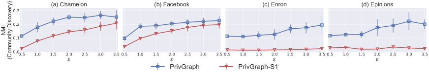
Figure 4: [Higher is better] Comparison of $\mathsf{PrivGraph}$ and $\mathsf{PrivGraph}$-S1. The columns represent the used datasets and the rows stand for different metrics. In each plot, the x-axis denotes the privacy budget $\varepsilon$, and the y-axis denotes the NMI value.

6 Related Work

6.1 Differentially Private Graph Analysis

Differentially private graph analysis can accomplish a series of statistical tasks on private data. Several strategies are designed for various downstream tasks, including degree distribution, community division, clustering coefficient, etc.

Degree Distribution. There are some works dedicated to the task of degree release [31, 50, 24]. In particular, lipschitz extensions and exponential mechanism are used in [50] for approximating the degree distribution of a sensitive graph. Hay et al. [24] designed an algorithm for publishing the degree distribution based on a constrained inference technique.

Topology Structure. Many studies have investigated the problem of protecting the topology structure of a graph [46, 28, 8, 71, 30], yet they are fundamentally different from $\mathsf{PrivGraph}$. First, for the problem definition, prior works  [8, 71, 30, 28] require both node attributes and edges, while $\mathsf{PrivGraph}$ only can touch the edges. Second, the results are published at different granularities. The related works [28, 46] output the community partitions, i.e., coarse granularity. $\mathsf{PrivGraph}$ generates a complete graph, i.e., fine granularity. Nguyen et al. [46] proposed to form a weighted graph by a filtering technique and then apply Louvain method to detect the communities. However, the random grouping of nodes in the beginning may cause a large deviation. Ji et al. [28] formulated the community detection of attributed graph as a maximum log-likelihood problem.

6.2 Privacy Attacks on Graph

There exist several works related to privacy attacks on graph data [72, 67, 73, 69, 16, 57]. According to different assumptions of the attacker’s ability, the inference attacks on edges could be divided into two categories. The first type of attacks make inferences based on the edge structure information [72, 67], i.e., nodes with higher structural similarity tend to be connected to each other. The second type of attacks attempt to reconstruct the original graph mainly based on the node features [69, 16], i.e., nodes with more similar attributes tend to link more closely.

For the first type of inference attacks on edges, $\mathsf{PrivGraph}$ could defend the attacks effectively since they do not violate edge-DP guarantees. For the second type of attacks, a single edge-DP technique may prove insufficient to thwart them since the attacker can infer edges barely based on the node features. In addition, it should be noticed that the ideal application scenarios of edge-DP require that all edges are independent of each other. In practice, different edges may be correlated, i.e., the presence of an edge might be inferred by other edges, which introduces greater challenges to privacy protection. The problem could be mitigated by applying $k$-edge DP [24] and considering the correlation between edges, which are promising directions for further improvements.

There are some de-anonymization attacks [36, 76] to re-identify nodes in an anonymized graph according to an auxiliary graph and a set of seed mappings, which is orthogonal to the privacy guarantee provided by edge-DP [24, 15].

6.3 Differentially Private Data Synthesis

There are some existing studies for other types of data.

Tabular Data. There are three mainstream methods to process tabular data: graphical model-based, game-based, and deep generative model-based. The core idea of graphical model-based methods is to estimate a graphical model which approximates the distribution of the original dataset under DP [42, 74]. The game-based methods regard the dataset synthesis problem as a zero-sum game [20, 59]. Deep generative model-based methods first train a deep generative model under DP and adopt the model to synthesize the dataset [2, 19].

Trajectory Data. There are a few works that investigate the synthesis of trajectory dataset while satisfying DP [25, 23, 5, 60]. He et al. [25] designed DPT method to discretize the space by various granularities and built multiple prefix trees. Wang et al. [60] proposed to dynamically choose between first-order and second-order Markov models to tradeoff noise error and correlation error. Du et al. [14] proposed LDPTrace for the local DP settings.

7 Conclusion

In this paper, we propose $\mathsf{PrivGraph}$ for publishing graph data under DP. By exploiting community information and considering the different characteristics of connections within and between communities, we extract the structure of the graph effectively and reconstruct it accurately. $\mathsf{PrivGraph}$ satisfies rigorous DP while achieving a balance between information loss and perturbation strength. Extensive experiments on six real-world datasets demonstrate the superiority of $\mathsf{PrivGraph}$. Compared with tailored private methods optimized for specific graph analysis tasks, $\mathsf{PrivGraph}$ still shows competitive results on some settings. We also explore the performance of $\mathsf{PrivGraph}$ on preserving small communities. Then, we empirically analyze the impact of hyper-parameters of $\mathsf{PrivGraph}$. For the practical applications, we show the advantage of $\mathsf{PrivGraph}$ on the influence maximization problem.

Appendix A Proof of Theorem 1

$\mathsf{PrivGraph}$ consists of three phases: Community division, information extraction, and graph reconstruction. Specifically, the community division phase includes two parts: i.e. community initialization and community adjustment. Next, we show that the components of $\mathsf{PrivGraph}$ are satisfying edge-DP.

Proof 1: Community Initialization satisfies $\varepsilon_{1}$-edge DP.

Proof.

In the process of community initialization, $\mathsf{PrivGraph}$ will perturb the true weighted graph generated from the random partitions. The perturbations of inner weights and outer weights are achieved by adding Laplace noise. Recalling Section 2.1, Laplace Mechanism can provide rigorous differential privacy guarantee. The inner and outer weights are independent of each other. According to the parallel composition, they can share the same privacy budget, i.e., $\varepsilon_{1}$. The consistency processing and community detection do not touch the true data and do not consume privacy budget. Hence, community initialization satisfies $\varepsilon_{1}$-edge DP. ∎

Proof 2: Community Adjustment satisfies $\varepsilon_{2}$-edge DP.

Proof.

$\mathsf{PrivGraph}$ adopts exponential mechanism to select the community for each node with the privacy budget of $\varepsilon_{a}=0.5\varepsilon_{2}$. We can assume that the two nodes corresponding to the only edge that differs between the original graph and the edge neighbor graph are $i$ and $j$.

For the nodes $i$ and $j$, given any inputs $v_{1},v_{2}$ ($v_{1}$ and $v_{2}$ differ by an edge), and output $o$, combining the probability equation of Section 2.1, we have

$$\frac{\mathsf{Pr}\left[\mathcal{A}_{q}(v_{1})=o\right]}{\mathsf{Pr}\left[\mathcal{A}_{q}(v_{2})=o\right]} \leq e^{\varepsilon_{a}},$$

where $q$ is the quality function, $\mathcal{O}$ is the set of all possible outputs, and $\Delta f_{c}$ is the global sensitivity.

For the other nodes except for node $i$ and node $j$, the inputs $v_{1}$ and $v_{2}$ are the same. Therefore, we have

$$\frac{\mathsf{Pr}\left[\mathcal{A}_{q}(v_{1})=o\right]}{\mathsf{Pr}\left[\mathcal{A}_{q}(v_{2})=o\right]}=e^{0}.$$

Based on the sequential composition, we can obtain $0.5\varepsilon_{2}+0.5\varepsilon_{2}+0=\varepsilon_{2}$. Hence, community adjustment satisfies $\varepsilon_{2}$-edge DP. ∎

Proof 3: Information Extraction satisfies $\varepsilon_{3}$-edge DP.

Proof.

In the phase of information extraction, the original degree sequence of intra-community and the true edge vector between communities are injected Laplace noise, respectively. Note that the degree sequence and the edge vector are disjoint subsets, they can be perturbed by the same privacy budget. The proof is similar to community initialization. Based on the parallel composition, we can obtain that information extraction satisfies $\varepsilon_{3}$-edge DP. ∎

Overall Privacy Budget. According to the above proofs, in the first phase, community initialization satisfies $\varepsilon_{1}$-edge DP and community adjustment satisfies $\varepsilon_{2}$-edge DP. The phase of information extraction satisfies $\varepsilon_{3}$-edge DP. In graph reconstruction, $\mathsf{PrivGraph}$ processes the perturbed data without consuming privacy budget. Hence, $\mathsf{PrivGraph}$ satisfies $\varepsilon$-edge DP in accordance with sequential composition.

Appendix B Complexity Analysis

In this section, we analyze the computational complexity of various methods, and quantitatively evaluate their running time and memory consumption.

Time Complexity. We provide the time complexity by analyzing each phase of the algorithms. The number of edges is $m$, and the number of nodes is $n$.

For $\mathsf{PrivGraph}$, the first phase is to divide the nodes into a number of communities by community initialization and community adjustment. The time complexity of community initialization is $\mathcal{O}(k_{1}^{2})$, where $k_{1}$ is the number of super-nodes. In the community adjustment, the time complexity is $\mathcal{O}(n)$. In information extraction, $\mathsf{PrivGraph}$ separately perturbs the original degree sequence of each community and the edge vector between communities. And the time cost of reconstruction is similar to that of information extraction. The time complexity of these two phases is $\mathcal{O}(k_{2}^{2})$, where $k_{2}$ is the number of communities. Above all, we have $\mathcal{O}(k_{1}^{2})+\mathcal{O}(n)+\mathcal{O}(k_{2}^{2})=\mathcal{O}(n+k_{1}^{2}+k_{2}^{2})<\mathcal{O}(n^{2})$, thus the total time complexity of $\mathsf{PrivGraph}$ is $\mathcal{O}(n^{2})$. In fact, the number of communities is much less than $n$, so the computation time is short.

$\mathsf{TmF}$ directly processes at most $2m$ 1-cells and 0-cells in the adjacency matrix. Therefore, the time complexity is $O(m)$, which increases with the number of edges linearly.

For $\mathsf{PrivHRG}$, it consists of three steps: HRG sampling, probability value perturbation, and graph generation. The first step is finding a suitable HRG by MCMC sampling, with the time complexity of $\mathcal{O}(n^{2}\log{n})$. The second step is adding Laplace noise to the probability values in the HRG and the time complexity is $\mathcal{O}(n)$. The final step is reconstructing the graph based on the probability between nodes. The time complexity is $\mathcal{O}(n^{2})$. $\mathcal{O}(n^{2}\log{n})+\mathcal{O}(n)+\mathcal{O}(n^{2})=\mathcal{O}(n^{2}\log{n})$.

$\mathsf{LDPGen}$ needs to group all nodes by $k$-means clustering, and to add noise to the formed matrix. The time complexity of $k$-means clustering is $\mathcal{O}(nkt)$, where $k$ is the number of clusters and $t$ is the number of iterations. The time complexity of adding noise is $\mathcal{O}(nk)$. Therefore, we can obtain $\mathcal{O}(nkt)+\mathcal{O}(nk)\approx\mathcal{O}(n^{2})$. The time complexity of $\mathsf{LDPGen}$ is $\mathcal{O}(n^{2})$.

$\mathsf{DER}$ includes three parts: Node relabeling, dense region exploration, and edge reconstruction. In the first part, $\mathsf{DER}$ generates $\frac{n}{2}$ candidate swaps for relabeling and each swap involves exactly two columns and two rows. Therefore, the time complexity of node relabeling is $\mathcal{O}(n^{2})$. In the procedure of dense region exploration, the complexity is determined by applying EM to select the splitting points. The time complexity of this procedure is $\mathcal{O}(n^{2})$. The third step is to reconstruct all leaving regions. The time complexity is $\mathcal{O}(n^{2})$. Hence, the overall time complexity of $\mathsf{DER}$ is $\mathcal{O}(n^{2})$.

Space Complexity. For $\mathsf{PrivGraph}$, it requires storing the information of edges and super-nodes. Therefore, the space complexity is $\mathcal{O}(m+n)$. The memory consumption of $\mathsf{TmF}$ is only related to the number of edges, i.e., $\mathcal{O}(m)$. For $\mathsf{PrivHRG}$, it needs to get the information of edges and maintain an HRG, requiring $\mathcal{O}(m+n)$ storage. The space complexity of $\mathsf{LDPGen}$ is $\mathcal{O}(n^{2})$ because it must store the connection information of all nodes to each cluster. The space complexity of $\mathsf{DER}$ is $\mathcal{O}(n^{2})$ due to the count summary matrix.

Empirical Evaluation. Table 4 and Table 5 show the running time and the memory consumption for all methods on the six datasets (see their details in Table 2). The empirical running time in Table 4 illustrates that the performance of $\mathsf{TmF}$ is best because it processes the cells in a linear time without further operations. The running time of $\mathsf{PrivGraph}$ and $\mathsf{LDPGen}$ are longer than $\mathsf{TmF}$ since they require grouping. $\mathsf{PrivHRG}$ and $\mathsf{DER}$ take much more time than $\mathsf{TmF}$, $\mathsf{LDPGen}$ and $\mathsf{PrivGraph}$. $\mathsf{PrivHRG}$ consumes huge time to sample an HRG, and $\mathsf{DER}$ spends lots of time dividing the adjacency matrix into small pieces.

Table 5 shows the memory consumption. $\mathsf{DER}$ is the highest. The reason is that $\mathsf{DER}$ needs to maintain a count matrix during the data processing. $\mathsf{LDPGen}$ is also high because it requires to storage the connection matrix of all nodes. The memory consumption of other methods is close because their space complexities are linear to $m$ or $n$.

Table 3: Comparison of computational complexity.

Methods	Time Complexity	Space Complexity
$\mathsf{TmF}$	$\mathcal{O}(m)$	$\mathcal{O}(m)$
$\mathsf{PrivHRG}$	$\mathcal{O}(n^{2}\log{n})$	$\mathcal{O}(m+n)$
$\mathsf{LDPGen}$	$\mathcal{O}(n^{2})$	$\mathcal{O}(n^{2})$
$\mathsf{DER}$	$\mathcal{O}(n^{2})$	$\mathcal{O}(n^{2})$
$\mathsf{PrivGraph}$	$\mathcal{O}(n^{2})$	$\mathcal{O}(m+n)$

Table 4: Comparison of running time (measured by seconds).

	Methods
Datasets	$\mathsf{TmF}$	$\mathsf{PrivGraph}$	$\mathsf{LDPGen}$	$\mathsf{DER}$	$\mathsf{PrivHRG}$
Chamelon	0.22s	1.47s	2.16s	136.41s	273.13s
Facebook	0.68s	4.13s	4.37s	383.81s	1580.24s
CA-HepPh	4.72s	17.84s	22.46s	2750.58s	4593.21s
Enron	31.20s	118.05s	61.41s	N/A	33677.63s
Epinions	105.46s	503.48s	312.84s	N/A	N/A
Gowalla	242.75s	2358.32s	N/A	N/A	N/A

Table 5: Comparison of memory consumption (measured by Megabytes).

	Methods
Datasets	$\mathsf{TmF}$	$\mathsf{PrivGraph}$	$\mathsf{LDPGen}$	$\mathsf{DER}$	$\mathsf{PrivHRG}$
Chamelon	30.88	36.46	61.52	151.74	50.93
Facebook	74.46	81.35	110.45	451.50	95.94
CA-HepPh	141.31	240.85	632.97	3139.57	546.06
Enron	210.18	913.13	4191.59	N/A	3586.20
Epinions	482.67	2563.14	14210.52	N/A	N/A
Gowalla	984.23	6811.05	N/A	N/A	N/A

Appendix C Experimental Setup

C.1 Datasets

The details of six datasets are as follows.

• Chamelon [54]. Collected from the English Wikipedia on the chamelon topic, it contains 2,277 nodes (i.e., articles) and 31,421 edges (i.e., mutual links).

• Facebook [39]. This dataset is collected from survey participants using a Facebook app. It contains 4,039 nodes (i.e., users) and 88,234 edges (i.e., connections).

• CA-HepPh [38]. CA-HepPh is from the e-print arXiv covering scientific collaborations between authors’ papers, which contains 12,008 nodes and 118,521 edges. The nodes represent the authors and the edges stand for the collaboration relationship.

• Enron [52]. The dataset is an email graph. Nodes represent the email accounts in Enron and edges represent the communications. It contains 33,696 nodes and 180,811 edges.

• Epinions [51]. The dataset is a trust network collected from a consumer review site. It contains 75,879 nodes (i.e., users) and 405,740 edges (i.e., trust relationships).

• Gowalla [10]. Gowalla is from a location-based social networking website, which contains 196,591 nodes (i.e., users) and 950,327 edges (i.e., friendships).

C.2 Evaluation Metrics

We evaluate the quality of the synthetic graph from five different aspects.

• Community Discovery. Here, we choose Normalized Mutual Information (NMI) [34] to measure the quality of community division. In particular, we apply the Louvain [3] method to acquire the partitions from the original graph and synthetic graph. Then we measure the difference between the group partitions by NMI.

  Given two partitions $A=\{A_{1},A_{2},\cdots A_{R}\}$ and $B=\{B_{1},B_{2},\cdots B_{S}\}$ of a graph $G=(V,E)$, the overlap between $A$ and $B$ can be represented through a contingency table $H$, where $H_{ij}$ stands for the number of nodes that belong to $A_{i}$ and $B_{j}$. Let $x_{i}$ (resp. $y_{j}$) denotes the sum of all elements in the $i$-th row (resp. $j$-th column) of the contingency table. We can obtain the NMI value between partitions $A$ and $B$ as follows.

  $$NMI(A,B)=\frac{-2\sum_{i=1}^{R}\sum_{j=1}^{S}H_{ij}\log\left(\frac{H_{ij}n}{x_{i}y_{j}}\right)}{\sum_{i=1}^{R}x_{i}\log\left(\frac{x_{i}}{n}\right)+\sum_{j=1}^{S}y_{j}\log\left(\frac{y_{j}}{n}\right)}$$

• Node Information. The eigenvector centrality (EVC) score is used to rank the nodes, which can identify the most influential nodes in a graph. We compare the percentage of common nodes in the top 1% most influential nodes of the original graph and the synthetic graph.

  $${Overlap}_{Node}=\frac{\left|N\cap\hat{N}\right|}{\left|N\right|},$$

  where $N$ and $\hat{N}$ stand for the node sets of the top 1% eigenvalues in the original graph and the synthetic graph. Besides, the Mean Absolute Error (MAE) of the top 1% most influential nodes’ EVC scores can be calculated as follows.

  $$MAE_{EVC}=\frac{1}{T}\sum_{i=1}^{T}\left|\hat{s}_{i}-s_{i}\right|,$$

  where $s_{i}$ and $\hat{s}_{i}$ are the EVC scores of the $i$-th most influential node in the original graph and the synthetic graph.

• Degree Distribution. The Kullback-Leibler (KL) divergence [33] is adopted to measure the difference of the degree distributions between the original graph and the synthetic graph.

  $$D_{KL}\left(P\parallel\hat{P}\right)=\sum_{x\in\mathcal{X}}P(x)\log\left(\frac{P(x)}{\hat{P}(x)}\right),$$

  where $P(x)$ and $\hat{P}(x)$ stand for the degree distributions of the original graph and the synthetic graph separately.

• Path Condition. We provide the Relative Error (RE) of the diameters, i.e., the maximum distance among all path-connected pairs of nodes, from the original graph and the synthetic graph.

  $${RE}_{Diam}=\frac{\left|\hat{D}-D\right|}{\max(\delta,D)},$$

  where ${D}$ and $\hat{D}$ are the diameters of the original graph and the synthetic graph, respectively, and $\delta$ is a small constant to avoid a zero denominator.

• Topology Structure. We compare the RE of the clustering coefficients and the modularities between the original graph and the synthetic graph. The RE of modularity can be obtained by:

  $${RE}_{Mod}=\frac{\left|\hat{Q}-Q\right|}{\max(\delta,Q)},$$

  where ${Q}$ and $\hat{Q}$ are the modularities of the original graph and the synthetic graph, respectively, and $\delta$ is a small constant to avoid a zero denominator. The RE of clustering coefficient can be calculated in a similar way.

  $${RE}_{CC}=\frac{\left|\hat{Y}-Y\right|}{\max(\delta,Y)},$$

  where ${Y}$ and $\hat{Y}$ are the clustering coefficients of the original graph and the synthetic graph, respectively, and $\delta$ is a small constant to avoid a zero denominator.

Appendix D Evaluation on Large Datasets

This section includes an additional evaluation of $\mathsf{PrivGraph}$ and its competitors using two large datasets. However, due to time and space constraints, it was difficult to run $\mathsf{DER}$, $\mathsf{PrivHRG}$, and $\mathsf{LDPGen}$ on these datasets. Therefore, we compared $\mathsf{PrivGraph}$ with $\mathsf{TmF}$ and $\mathsf{LDPGen}$ on the Epinions dataset, and compared $\mathsf{PrivGraph}$ with $\mathsf{TmF}$ on the Gowalla dataset. The experimental results are shown in Figure 5 and Figure 6, while the diameter metric is not included due to the lengthy calculation time.

$\mathsf{PrivGraph}$ continues to exhibit significant advantages over other methods when dealing with large datasets. This is due to its ability to group similar nodes into the same community, thus preserving the original graph structure. Additionally, $\mathsf{PrivGraph}$ is able to extract both intra- and inter-community information at different levels of granularity, and use appropriate reconstruction methods. As a result, $\mathsf{PrivGraph}$ generally outperforms other methods in most scenarios. However, when the privacy budget is limited, the performance of certain metrics may be impacted due to the strong perturbation. In contrast, $\mathsf{LDPGen}$ achieves superior results compared to $\mathsf{TmF}$ by reducing the dimensionality of the original graph through clustering. $\mathsf{TmF}$, on the other hand, perturbs the entire adjacency matrix, and requires a large privacy budget to achieve competitive results.

Figure 5: Performance of six metrics on the Epinions dataset. In each plot, the x-axis denotes the privacy budget $\varepsilon$, and the y-axis denotes the performance. For the first two metrics of the first row, higher is better. For the other metrics, lower is better.

Figure 6: Performance of six metrics on the Gowalla dataset. In each plot, the x-axis denotes the privacy budget $\varepsilon$, and the y-axis denotes the performance. For the first two metrics of the first row, higher is better. For the other metrics, lower is better.

Appendix E Ablation Study

E.1 Impact of the Number of Nodes for Community Initialization

Recalling Section 4.3, the number of nodes $N$ in community initialization controls the initial scale of the communities. If $N$ is too small, there will generate a large number of communities, and the perturbation noise tends to overwhelm the true information, especially when the privacy budget is small. If $N$ is too high, it will aggravate the error caused by random division and cannot obtain a precise partition. Therefore, a suitable $N$ value is significant to balance the above two factors. However, the theoretical selection of $N$ is hard due to the following two reasons. Firstly, the graph data has various structures in practice, e.g., the number of communities is usually different in graph datasets. In addition, $\mathsf{PrivGraph}$ can access the original graph by using privacy budget, yet the complexity of estimating an accurate $N$ brings a high privacy budget overhead, which is not cost-effective for other processes of $\mathsf{PrivGraph}$.

In Figure 7, we show the performance of $\mathsf{PrivGraph}$ under different combinations of $N$ and $\varepsilon$. When the privacy budget is small, the noise has an significant impact on the final results, and a larger $N$ is helpful to achieve higher accuracy because it reduces the number of initial communities. If the privacy budget is large enough, the injected noise has a limited effect, and the error from random division will play a dominant role. In this case, a smaller $N$ facilitates a better performance.

We find that there exists no fixed optimal $N$ for all privacy budgets and datasets. For example, when the privacy budget is $0.5$, $\mathsf{PrivGraph}$ usually performs better as $N$ increases. The reason is that the privacy budget is small and the perturbation noise cannot be ignored. When the privacy budget is up to $2$, with the increase of $N$, many metrics perform better first and then worse, such as NMI, clustering coefficient, and modularity. This is caused by the combined effect of perturbation noise and random division error. If the privacy budget is $3.5$, a smaller $N$ can achieve higher results on the Chamelon and Facebook datasets because the number of communities formed is lower than the other two datasets. The influence of random division error is significant when the privacy budget is large. Overall, $\mathsf{PrivGraph}$ maintains competitive synthetic quality when $N=20$, thus we set $N=20$ throughout the experiments.

Figure 7: Impact of the number of nodes for community initialization. The columns represent the used datasets, and the rows stand for different metrics. In each plot, the x-axis denotes the number of nodes $N$, and the y-axis denotes the performance. For the first two rows, higher is better. For the last five rows, lower is better.

Figure 8: Impact of privacy budget allocation. The columns represent the used datasets, and the rows stand for different metrics. In each plot, the x-axis denotes the ratio of $\varepsilon_{1}$, the y-axis denotes the ratio of $\varepsilon_{2}$ $(\varepsilon_{3}=\varepsilon-\varepsilon_{1}-\varepsilon_{2})$, and the values in the grid denote the performance. For the first two rows, higher is better. For the last five rows, lower is better.

E.2 Impact of the Privacy Budget Allocation

Recalling Section 4.2, the entire privacy budget is divided into three parts: Community initialization ($\varepsilon_{1}$), community adjustment ($\varepsilon_{2}$) and information extraction ($\varepsilon_{3}$). We vary the ratio of $\varepsilon_{1}$ and $\varepsilon_{2}$ to $\varepsilon$ from $0.1$ to $0.8$ with step size $0.1$. Then $\varepsilon_{3}$ can be calculated by $\varepsilon-\varepsilon_{1}-\varepsilon_{2}$. Figure 8 shows the impact of privacy budget allocation on four datasets and seven metrics when the privacy budget is $2$.

We observe that the allocation ratio has an obvious influence on the experiment results. For the overlap metric, if both $\varepsilon_{1}$ and $\varepsilon_{2}$ are small, $\mathsf{PrivGraph}$ cannot achieve high overlap ratios. The reason is that the overlap ratio depends on the quality of community division. If the communities obtained are not accurate, it is difficult to identify the nodes with high eigenvalues. If the ratio of $\varepsilon_{3}$ is small, $\mathsf{PrivGraph}$ cannot obtain the best performance since the extracted information is injected lots of noise. For the modularity metric, the behavior of $\mathsf{PrivGraph}$ is poor when $\varepsilon_{1}$ and $\varepsilon_{2}$ are low, which is similar to the overlap results. The recovery of modularity also requires accurate community partitions. The impact of the perturbation noise from information extraction is negligible if we have proper partitions.

Based on the above observations, the impact of the budget allocation strategy varies on different datasets. Considering the universal applicability of $\mathsf{PrivGraph}$, we set $\varepsilon_{1}=\varepsilon_{2}=\varepsilon_{3}=\frac{1}{3}\varepsilon$ for all experiments.

E.3 Impact of the Resolution

Recalling Section 2.3, modularity optimization may fail to detect small communities, i.e., resolution limit. Thus, in this section, we compare the performance of $\mathsf{PrivGraph}$ under the resolution parameter $t$ ranging from 0.2 to 1.5. Figure 9 illustrates the impact of the resolution parameter on four datasets and three metrics.

We observe that the resolution parameter $t$ has a significant impact on the final results. For the first metric, as the resolution parameter increases, the overlap ratio shows a tendency of increasing and then decreasing. The reason is that a too small $t$ will lead to excessive partitions, which breaks the connections between the influential nodes and other nodes, while the community will be insufficiently divided if $t$ is too large. For the degree distribution, the KL divergence shows a decreasing trend as $t$ increases since $\mathsf{PrivGraph}$ extracts the degree information within the community. For the clustering coefficient, with the increase of the resolution parameter, the RE decreases and then increases. The reason is similar to that of the overlap metric. If the resolution parameter is too small, it will introduce a large amount of noise between the communities, and a too-large resolution parameter cannot detect the community structure accurately. Therefore, a suitable resolution parameter $t$ is essential to balance the effects of the above two parts. $\mathsf{PrivGraph}$ shows consistently excellent performance when the resolution parameter $t$ is around 1.

Figure 9: Impact of the resolution. The columns represent the used datasets and the rows stand for different metrics. In each plot, the x-axis denotes the privacy budget $\varepsilon$, and the y-axis denotes the performance. For the first row, higher is better. For the last two rows, lower is better.

Appendix F Case Study: Influence Maximization

Figure 10: [Higher is better] The influence spread of different methods. The captions represent the name of the used datasets. In each plot, the x-axis denotes the privacy budget $\varepsilon$, the y-axis denotes the influence spread, and the black dashed line denotes the results on the original graph (without DP guarantee).

In this section, we apply $\mathsf{PrivGraph}$ to the Influence Maximization (IM) problem [12], which aims to locate the nodes of maximum impact from a given graph. A typical application of IM is viral marketing, where a company tries to promote a new product in some targeted individuals [40].

Setup. We adopt a classical method, called Degree-Discount (DD) [7], to find the top 20 of most influential nodes on the synthetic graph. Then, we compare the influence spreads of the selected nodes from different methods by leveraging the standard Independent Cascade (IC) [32] model with $p=0.01$ on the original graph, where the higher influence spread values mean more accurate location of the most influential nodes.

Observations. Figure 10 illustrates the influence spread of the most influential nodes obtained by various methods. We observe that the influence spread obtained by $\mathsf{PrivGraph}$ is the highest in most cases. Recalling Section 4.3 and Section 4.4, $\mathsf{PrivGraph}$ groups the nodes with similar connection structures into a community, and then extracts the intra-information from each community separately. In this way, $\mathsf{PrivGraph}$ recovers both the nodes’ degree and graph structure, which is essential for discovering influential nodes. When the privacy budget is limited, e.g., $\varepsilon=0.5$, the privacy budget is too small to accurately detect the communities, impacting the final influence spread.

The performance of $\mathsf{LDPGen}$ is not stable on the four datasets. For the last two datasets, the number of high-degree nodes is larger, which is less susceptible to noise. The performance of $\mathsf{PrivHRG}$ is better than $\mathsf{TmF}$ and $\mathsf{DER}$. Since $\mathsf{PrivHRG}$ encodes the original graph into a tree structure and rebuilds the graph based on the connection probability between nodes, $\mathsf{PrivHRG}$ mitigates the perturbation impact on the original degree distributions. Recalling Section 5.2, $\mathsf{DER}$ performs better than $\mathsf{PrivHRG}$ and $\mathsf{TmF}$ on the overlap of nodes, while poorly on the influence maximization. The reason for the inconsistency is that Degree-Discount [7] finds the set of seed nodes mainly from the perspective of node degree rather than eigenvalues.

References

- [1] W. Aiello, F. Chung, and L. Lu. A Random Graph Model for Massive Graphs. In Proceedings of the thirty-second Annual ACM Symposium on Theory of Computing, pages 171–180, 2000.
- [2] B. K. Beaulieu-Jones, Z. S. Wu, C. Williams, R. Lee, S. P. Bhavnani, J. B. Byrd, and C. S. Greene. Privacy-Preserving Generative Deep Neural Networks Support Clinical Data Sharing. Circulation: Cardiovascular Quality and Outcomes, 12(7):e005122, 2019.
- [3] V. D. Blondel, J.-L. Guillaume, R. Lambiotte, and E. Lefebvre. Fast Unfolding of Communities in Large Networks. Journal of Statistical Mechanics: Theory and Experiment, 2008(10):P10008, 2008.
- [4] M. Chen, Z. Zhang, T. Wang, M. Backes, M. Humbert, and Y. Zhang. Graph Unlearning. In Proceedings of the 2022 ACM SIGSAC Conference on Computer and Communications Security, 2022.
- [5] R. Chen, G. Acs, and C. Castelluccia. Differentially Private Sequential Data Publication via Variable-Length N-Grams. In Proceedings of the 2012 ACM Conference on Computer and Communications Security, pages 638–649, 2012.
- [6] R. Chen, B. Fung, P. S. Yu, and B. C. Desai. Correlated Network Data Publication via Differential Privacy. The VLDB Journal, 23(4):653–676, 2014.
- [7] W. Chen, Y. Wang, and S. Yang. Efficient Influence Maximization in Social Networks. In Proceedings of the 15th ACM SIGKDD International Conference on Knowledge Discovery and Data Mining, pages 199–208, 2009.
- [8] X. Chen, S. Mauw, and Y. Ramírez-Cruz. Publishing Community-Preserving Attributed Social Graphs with a Differential Privacy Guarantee. Proceedings on Privacy Enhancing Technologies, 2020(4):131–152, 2020.
- [9] J. Cheng, A. W.-c. Fu, and J. Liu. K-Isomorphism: Privacy Preserving Network Publication against Structural Attacks. In Proceedings of the 2010 ACM SIGMOD International Conference on Management of data, pages 459–470, 2010.
- [10] E. Cho, S. A. Myers, and J. Leskovec. Friendship and Mobility: User Movement in Location-Based Social Networks. In Proceedings of the 17th ACM SIGKDD International Conference on Knowledge Discovery and Data Mining, pages 1082–1090, 2011.
- [11] A. Clauset, C. Moore, and M. E. Newman. Hierarchical Structure and the Prediction of Missing Links in Networks. Nature, 453(7191):98–101, 2008.
- [12] P. Domingos and M. Richardson. Mining the Network Value of Customers. In Proceedings of the seventh ACM SIGKDD International Conference on Knowledge Discovery and Data Mining, pages 57–66, 2001.
- [13] L. Du, Z. Zhang, S. Bai, C. Liu, S. Ji, P. Cheng, and J. Chen. AHEAD: Adaptive Hierarchical Decomposition for Range Query under Local Differential Privacy. In Proceedings of the 2021 ACM SIGSAC Conference on Computer and Communications Security, pages 1266–1288, 2021.
- [14] Y. Du, Y. Hu, Z. Zhang, Z. Fang, L. Chen, B. Zheng, and Y. Gao. LDPTrace: Locally Differentially Private Trajectory Synthesis. In VLDB, 2023.
- [15] C. Dwork, F. McSherry, K. Nissim, and A. Smith. Calibrating Noise to Sensitivity in Private Data Analysis. In Theory of Cryptography Conference, pages 265–284. Springer, 2006.
- [16] N. Eagle, A. Pentland, and D. Lazer. Inferring Friendship Network Structure by Using Mobile Phone Data. Proceedings of the National Academy of Sciences, 106(36):15274–15278, 2009.
- [17] S. Eubank, V. A. Kumar, M. V. Marathe, A. Srinivasan, and N. Wang. Structural and Algorithmic Aspects of Massive Social Networks. In Proceedings of the fifteenth Annual ACM-SIAM Symposium on Discrete Algorithms, pages 718–727, 2004.
- [18] S. Fortunato and M. Barthelemy. Resolution Limit in Community Detection. Proceedings of the National Academy of Sciences, 104(1):36–41, 2007.
- [19] L. Frigerio, A. S. d. Oliveira, L. Gomez, and P. Duverger. Differentially Private Generative Adversarial Networks for Time Series, Continuous, and Discrete Open Data. In IFIP International Conference on ICT Systems Security and Privacy Protection, pages 151–164. Springer, 2019.
- [20] M. Gaboardi, E. J. G. Arias, J. Hsu, A. Roth, and Z. S. Wu. Dual Query: Practical Private Query Release for High Dimensional Data. In International Conference on Machine Learning, pages 1170–1178. PMLR, 2014.
- [21] M. Girvan and M. E. Newman. Community Structure in Social and Biological Networks. Proceedings of the National Academy of Sciences, 99(12):7821–7826, 2002.
- [22] R. Guimera, M. Sales-Pardo, and L. A. N. Amaral. Modularity from Fluctuations in Random Graphs and Complex Networks. Physical Review E, 70(2):025101, 2004.
- [23] M. E. Gursoy, L. Liu, S. Truex, L. Yu, and W. Wei. Utility-Aware Synthesis of Differentially Private and Attack-Resilient Location Traces. In Proceedings of the 2018 ACM SIGSAC Conference on Computer and Communications Security, pages 196–211, 2018.
- [24] M. Hay, C. Li, G. Miklau, and D. Jensen. Accurate Estimation of the Degree Distribution of Private Networks. In 2009 Ninth IEEE International Conference on Data Mining, pages 169–178. IEEE, 2009.
- [25] X. He, G. Cormode, A. Machanavajjhala, C. M. Procopiuc, and D. Srivastava. DPT: Differentially Private Trajectory Synthesis Using Hierarchical Reference Systems. Proceedings of the VLDB Endowment, 8(11):1154–1165, 2015.
- [26] J. Imola, T. Murakami, and K. Chaudhuri. Locally Differentially Private Analysis of Graph Statistics. In 30th USENIX Security Symposium (USENIX Security 21), pages 983–1000, 2021.
- [27] S. Ji, P. Mittal, and R. Beyah. Graph Data Anonymization, De-Anonymization Attacks, and De-Anonymizability Quantification: A Survey. IEEE Communications Surveys & Tutorials, 19(2):1305–1326, 2016.
- [28] T. Ji, C. Luo, Y. Guo, Q. Wang, L. Yu, and P. Li. Community Detection in Online Social Networks: A Differentially Private and Parsimonious Approach. IEEE transactions on Computational Social Systems, 7(1):151–163, 2020.
- [29] F. Jiang, C. K. Leung, and A. G. Pazdor. Big Data Mining of Social Networks for Friend Recommendation. In 2016 IEEE/ACM International Conference on Advances in Social Networks Analysis and Mining (ASONAM), pages 921–922. IEEE, 2016.
- [30] Z. Jorgensen, T. Yu, and G. Cormode. Publishing Attributed Social Graphs with Formal Privacy Guarantees. In Proceedings of the 2016 International Conference on Management of Data, pages 107–122, 2016.
- [31] S. P. Kasiviswanathan, K. Nissim, S. Raskhodnikova, and A. Smith. Analyzing Graphs with Node Differential Privacy. In Theory of Cryptography Conference, pages 457–476. Springer, 2013.
- [32] D. Kempe, J. Kleinberg, and É. Tardos. Maximizing the Spread of Influence through a Social Network. In Proceedings of the ninth ACM SIGKDD International Conference on Knowledge Discovery and Data Mining, pages 137–146, 2003.
- [33] S. Kullback. Information Theory and Statistics. Courier Corporation, 1997.
- [34] T. O. Kvalseth. Entropy and Correlation: Some Comments. IEEE Transactions on Systems, Man, and Cybernetics, 17(3):517–519, 1987.
- [35] R. Lambiotte, J.-C. Delvenne, and M. Barahona. Laplacian Dynamics and Multiscale Modular Structure in Networks. CoRR, abs/0812.1770, 2008.
- [36] W.-H. Lee, C. Liu, S. Ji, P. Mittal, and R. B. Lee. How to Quantify Graph De-Anonymization Risks. In Information Systems Security and Privacy, pages 84–104, 2017.
- [37] J. Leskovec, D. Huttenlocher, and J. Kleinberg. Signed Networks in Social Media. In Proceedings of the SIGCHI Conference on Human Factors in Computing Systems, pages 1361–1370, 2010.
- [38] J. Leskovec, J. Kleinberg, and C. Faloutsos. Graph Evolution: Densification and Shrinking Diameters. ACM transactions on Knowledge Discovery from Data (TKDD), 1(1):2–es, 2007.
- [39] J. Leskovec and J. Mcauley. Learning to Discover Social Circles in Ego Networks. Advances in Neural Information Processing Systems, 25, 2012.
- [40] Y. Li, J. Fan, Y. Wang, and K.-L. Tan. Influence Maximization on Social Graphs: A Survey. IEEE Transactions on Knowledge and Data Engineering, 30(10):1852–1872, 2018.
- [41] D. Lusseau and M. E. Newman. Identifying the Role that Animals Play in Their Social Networks. Proceedings of the Royal Society of London. Series B: Biological Sciences, 271(suppl_6):S477–S481, 2004.
- [42] R. McKenna, D. Sheldon, and G. Miklau. Graphical-Model Based Estimation and Inference for Differential Privacy. In International Conference on Machine Learning, pages 4435–4444. PMLR, 2019.
- [43] F. McSherry and K. Talwar. Mechanism Design via Differential Privacy. In 48th Annual IEEE Symposium on Foundations of Computer Science (FOCS’07), pages 94–103. IEEE, 2007.
- [44] P. J. Mucha and M. A. Porter. Communities in Multislice Voting Networks. Chaos: An Interdisciplinary Journal of Nonlinear Science, 20(4):041108, 2010.
- [45] H. H. Nguyen, A. Imine, and M. Rusinowitch. Differentially Private Publication of Social Graphs at Linear Cost. In 2015 IEEE/ACM International Conference on Advances in Social Networks Analysis and Mining (ASONAM), pages 596–599. IEEE, 2015.
- [46] H. H. Nguyen, A. Imine, and M. Rusinowitch. Detecting Communities under Differential Privacy. In Proceedings of the 2016 ACM on Workshop on Privacy in the Electronic Society, pages 83–93, 2016.
- [47] M. A. Porter, J.-P. Onnela, P. J. Mucha, et al. Communities in Networks. Notices of the AMS, 56(9):1082–1097, 2009.
- [48] J. Qian, X.-Y. Li, C. Zhang, L. Chen, T. Jung, and J. Han. Social Network De-Anonymization and Privacy Inference with Knowledge Graph Model. IEEE Transactions on Dependable and Secure Computing, 16(4):679–692, 2017.
- [49] Z. Qin, T. Yu, Y. Yang, I. Khalil, X. Xiao, and K. Ren. Generating Synthetic Decentralized Social Graphs with Local Differential Privacy. In Proceedings of the 2017 ACM SIGSAC Conference on Computer and Communications Security, pages 425–438, 2017.
- [50] S. Raskhodnikova and A. Smith. Lipschitz Extensions for Node-Private Graph Statistics and the Generalized Exponential Mechanism. In 2016 IEEE 57th Annual Symposium on Foundations of Computer Science (FOCS), pages 495–504. IEEE, 2016.
- [51] M. Richardson, R. Agrawal, and P. Domingos. Trust Management for the Semantic Web. In The Semantic Web-ISWC 2003: Second International Semantic Web Conference, Sanibel Island, FL, USA, October 20-23, 2003. Proceedings 2, pages 351–368. Springer, 2003.
- [52] R. A. Rossi and N. K. Ahmed. The Network Data Repository with Interactive Graph Analytics and Visualization. In AAAI, 2015.
- [53] M. Rosvall and C. T. Bergstrom. Maps of Random Walks on Complex Networks Reveal Community Structure. Proceedings of the National Academy of Sciences, 2008.
- [54] B. Rozemberczki, C. Allen, and R. Sarkar. Multi-Scale Attributed Node Embedding. Journal of Complex Networks, 9(2):cnab014, 2021.
- [55] A. Sala, X. Zhao, C. Wilson, H. Zheng, and B. Y. Zhao. Sharing Graphs Using Differentially Private Graph Models. In Proceedings of the 2011 ACM SIGCOMM Conference on Internet Measurement Conference, pages 81–98, 2011.
- [56] D. Sharma, R. Shukla, A. K. Giri, and S. Kumar. A Brief Review on Search Engine Optimization. In 2019 9th International Conference on Cloud Computing, Data Science & Engineering, pages 687–692. IEEE, 2019.
- [57] Y. Shen, Y. Han, Z. Zhang, M. Chen, T. Yu, M. Backes, Y. Zhang, and G. Stringhini. Finding MNEMON: Reviving Memories of Node Embeddings. In ACM CCS, 2022.
- [58] H. Sun, X. Xiao, I. Khalil, Y. Yang, Z. Qin, H. Wang, and T. Yu. Analyzing Subgraph Statistics from Extended Local Views with Decentralized Differential Privacy. In Proceedings of the 2019 ACM SIGSAC Conference on Computer and Communications Security, 2019.
- [59] G. Vietri, G. Tian, M. Bun, T. Steinke, and S. Wu. New Oracle-Efficient Algorithms for Private Synthetic Data Release. In International Conference on Machine Learning, pages 9765–9774. PMLR, 2020.
- [60] H. Wang, Z. Zhang, T. Wang, S. He, M. Backes, J. Chen, and Y. Zhang. PrivTrace: Differentially Private Trajectory Synthesis by Adaptive Markov Model. In USENIX Security Symposium 2023, 2023.
- [61] T. Wang, J. Q. Chen, Z. Zhang, D. Su, Y. Cheng, Z. Li, N. Li, and S. Jha. Continuous Release of Data Streams under both Centralized and Local Differential Privacy. In ACM CCS, 2021.
- [62] T. Wang, M. Lopuhaä-Zwakenberg, Z. Li, B. Skoric, and N. Li. Locally Differentially Private Frequency Estimation with Consistency. In Proceedings of the 27th Annual Network and Distributed System Security Symposium, 2020.
- [63] Y. Wang and X. Wu. Preserving Differential Privacy in Degree-Correlation based Graph Generation. Transactions on Data Privacy, 6(2):127, 2013.
- [64] Y. Wang, L. Xie, B. Zheng, and K. C. Lee. High Utility K-Anonymization for Social Network Publishing. Knowledge and Information Systems, 41(3):697–725, 2014.
- [65] S. Wasserman and K. Faust. Social Network Analysis: Methods and Applications. Cambridge university press, 1994.
- [66] C. Wei, S. Ji, C. Liu, W. Chen, and T. Wang. AsgLDP: Collecting and Generating Decentralized Attributed Graphs With Local Differential Privacy. IEEE Transactions on Information Forensics and Security, 15:3239–3254, 2020.
- [67] X. Xian, T. Wu, Y. Liu, W. Wang, C. Wang, G. Xu, and Y. Xiao. Towards Link Inference Attack against Network Structure Perturbation. Knowledge-Based Systems, 218:106674, 2021.
- [68] Q. Xiao, R. Chen, and K.-L. Tan. Differentially Private Network Data Release via Structural Inference. In Proceedings of the 20th ACM SIGKDD International Conference on Knowledge Discovery and Data Mining, pages 911–920, 2014.
- [69] C. Yang, L. Zhong, L.-J. Li, and L. Jie. Bi-Directional Joint Inference for User Links and Attributes on Large Social Graphs. In Proceedings of the 26th International Conference on World Wide Web Companion, pages 564–573, 2017.
- [70] Q. Ye, H. Hu, M. H. Au, X. Meng, and X. Xiao. Towards Locally Differentially Private Generic Graph Metric Estimation. In 2020 IEEE 36th International Conference on Data Engineering (ICDE), pages 1922–1925. IEEE, 2020.
- [71] S. Zhang, W. Ni, and N. Fu. Community Preserved Social Graph Publishing with Node Differential Privacy. In 2020 IEEE International Conference on Data Mining (ICDM), pages 1400–1405. IEEE, 2020.
- [72] Y. Zhang, M. Humbert, B. Surma, P. Manoharan, J. Vreeken, and M. Backes. Towards Plausible Graph Anonymization. In Proceedings of the 27th Annual Network and Distributed System Security Symposium, 2020.
- [73] Z. Zhang, M. Chen, M. Backes, Y. Shen, and Y. Zhang. Inference Attacks Against Graph Neural Networks. In USENIX Security Symposium 2022, 2022.
- [74] Z. Zhang, T. Wang, J. Honorio, N. Li, M. Backes, S. He, J. Chen, and Y. Zhang. PrivSyn: Differentially Private Data Synthesis. In USENIX Security Symposium 2021, 2021.
- [75] Z. Zhang, T. Wang, N. Li, S. He, and J. Chen. CALM: Consistent Adaptive Local Marginal for Marginal Release under Local Differential Privacy. In Proceedings of the 2018 ACM SIGSAC Conference on Computer and Communications Security, pages 212–229, 2018.
- [76] Y. Zhao and I. Wagner. Using Metrics Suites to Improve the Measurement of Privacy in Graphs. IEEE Transactions on Dependable and Secure Computing, 19(1):259–274, 2020.