A Budget-Adaptive Allocation Rule for Optimal Computing Budget Allocation

Abstract

Simulation-based ranking and selection (R&S) is a popular technique for optimizing discrete-event systems (DESs). It evaluates the mean performance of system designs by simulation outputs and aims to identify the best system design from a finite set of alternatives by intelligently allocating a limited simulation budget. In R&S, the optimal computing budget allocation (OCBA) is an efficient budget allocation rule that asymptotically maximizes the probability of correct selection (PCS). However, the OCBA allocation rule ignores the impact of budget size, which plays an important role in finite budget allocation. To address this, we develop a budget allocation rule that is adaptive to the simulation budget. Theoretical results show that the proposed allocation rule can dynamically determine the ratio of budget allocated to designs based on different simulation budgets and achieve asymptotic optimality. Furthermore, the finite-budget properties possessed by our proposed allocation rule highlight the significant differences between finite budget and sufficiently large budget allocation strategies. Based on the proposed budget-adaptive allocation rule, two heuristic algorithms are developed. In the numerical experiments, we use both synthetic examples and a case study to show the superior efficiency of our proposed allocation rule.

I Introduction

Discrete-event systems (DESs) are a widely-used technical abstraction for complex systems (see [1]), such as traffic control systems, manufacturing systems, and communication systems. When the complexity of DESs is high and analytical models are unavailable, a powerful tool for evaluating the performance of DESs is discrete-event system simulation (see [2]). In this paper, we consider a problem of identifying the best system design from a finite set of competing alternatives, where “best” is defined with respect to the smallest or largest mean performance. The performance of each design is unknown and can be learnt by samples, i.e., by the sample mean of simulation outputs. Such problem is often called statistical ranking and selection (R&S) problem (see [3, 4, 5]) or Ordinal Optimization (OO) problem (see [6] and [7]).

In R&S, sampling efficiency is of significant concern as the simulation budget is often limited by its high expense. For example, the running time for a single simulation replication of the 24-hour dynamics of the scheduling process in a transportation network with 20 intersections can be about 2 hours, and it can take 30 minutes to obtain an accurate estimate of a maintenance strategy’s average cost by running 1,000 independent simulation replications for a re-manufacturing system (see [7]). With finite simulation replications, it is impossible to guarantee a correct selection of the best design occurs with probability 1. This nature of the problem motivates the need of implementing R&S techniques to intelligently allocate simulation replications to designs for efficiently identifying the best design. In our problem, we consider a fixed budget setting, and the probability of correct selection (PCS), a primary criterion in R&S literature, is used to measure the quality of budget allocation rules. The goal is to derive a budget allocation rule that can maximize the PCS subjecting to a constraint simulation budget.

Although the simulation budget is limited and of vital importance, many R&S algorithms allocate a simulation budget either by asymptotically optimal or by one-step-ahead optimal allocation rules, both of which can not adapt to the simulation budget. Intuitively, we argue that a desirable budget allocation rule should be adaptive to the simulation budget. We use an example to illustrate the significant impact of simulation budget on the optimal budget allocation rule. Suppose that there are three designs (design 1, 2, and 3) with normal sampling distributions $N(1,6^{2})$, $N(2,6^{2})$, and $N(3,6^{2})$, respectively. The optimal budget allocation ratios, which can maximize the PCS, are derived by using an exhaustive search, and the PCS is estimated through Monte Carlo simulation. As shown in table I, the optimal budget allocation ratios can be drastically different when the simulation budget changes. This observation is also consistent with theoretical analyses on the optimal budget allocation rules under different simulation budgets. The optimal computing budget allocation (OCBA) asymptotically maximizes the PCS, and it tends to allocate large budget allocation ratios to competitive designs, where competitive designs include the best design and non-best designs that are hard to distinguish from the best (see [8]). However, when the simulation budget is relatively small, assigning large budget allocation ratios to competitive designs, according to the OCBA allocation rule, may decease the PCS (see [9]). Such scenario is referred to as the low-confidence scenario (see [10]) and also takes place in the expected value of information (EVI) in [11] and knowledge gradient (KG) polices in [12]. To avoid the decrease of PCS, the budget allocation ratios of competitive designs should be discounted and the budget allocation ratios of non-competitive designs should be increased (see [10] and [13]). This counter-intuitive result emphasizes the significant impact of simulation budget on the budget allocation rule. It motivates the need of deriving a desirable budget allocation rule that considers and adapts to the simulation budget.

TABLE I: Optimal static budget allocation ratios for three alternative designs under different simulation budgets

Simulation budget	Design 1	Design 2	Design 3
20	0.100	0.350	0.550
50	0.320	0.360	0.320
200	0.400	0.365	0.235
500	0.436	0.396	0.168

In this work, we consider a simulation-based R&S problem under a fixed budget setting. We formulate the budget allocation problem as an OCBA problem. Instead of assuming a sufficiently large simulation budget like OCBA does, we consider a finite simulation budget and derive an allocation rule that is adaptive to the simulation budget. Theoretical results show that, compared with the OCBA allocation rule in [8], our proposed allocation rule can discount the budget allocation ratios of non-best designs that are hard to distinguish from the best design while increase the budget allocation ratios of those that are easy to distinguish. These adjustments are based on the simulation budget. When the simulation budget goes to infinity, the proposed allocation rule reduces to the OCBA allocation rule, which is asymptotically optimal. The finite-budget properties possessed by our proposed allocation rule highlight the significant differences between finite budget and sufficiently large budget allocation strategies (see [9] and [13]).

To summarize, the main contributions of this paper are as follows:

• We incorporate the simulation budget into the budget allocation rule and explicitly present the distinct behavior of the proposed budget-adaptive allocation rule under both finite and sufficiently large budgets. The finite-budget properties possessed by our proposed allocation rule is important as the simulation budget is often limited in practice.

• Based on two approaches implementing the proposed budget-adaptive allocation rule, we design two heuristic algorithms, called final-budget anchorage allocation (FAA) and dynamic anchorage allocation (DAA). Specifically, FAA fixes the simulation budget to maximize the final PCS while DAA dynamically anchors the next simulation replication to maximize the PCS after the additional allocation.

II Related Literature

In simulation optimization, the objective is to select the best design among a finite set of alternatives with respect to a performance metric, e.g., PCS. Due to the noisy simulation outputs, it is impossible to surely identify the best design within finite observations. Therefore, a strategy that intends to intelligently allocate simulation replications among designs is supposed to be developed. This problem falls into the actively studied ranking and selection (R&S) problem.

There are two branches of problem settings in R&S literature. One is fixed-confidence setting and the other is fixed-budget setting. Fixed-confidence R&S primarily focuses on the indifference zone (IZ) formulation and tries to guarantee a pre-specified level of PCS while using as little simulation budget as possible (see [14]). In later work, the IZ formulation is implemented to develop Frequentist procedures that can adapt to fully sequential setting (see [15, 16, 17]). Indifference-zone-free procedure that does not require an IZ parameter is proposed in [18]. More recently, IZ procedures for large-scale R&S problems in parallel computing environment are developed (see [19, 20, 21]). The fixed-budget R&S procedures are designed to optimize a certain kind of performance metric by efficiently allocating a fixed simulation budget. In the fixed-budget setting, there are procedures that allocate a simulation budget according to an asymptotically optimal allocation rule, such as OCBA (see [8]), the large deviation allocation (see [22]), and the optimal expected opportunity cost allocation (OEA) (see [23]); and procedures that myopically maximize the expected one-step-ahead improvement, such as the expected value of information (EVI) (see [11]), the knowledge gradient (see [12]), and the approximately optimal myopic allocation policy (AOMAP) (see [24]). In particular, the approximately optimal allocation policy (AOAP) achieves both one-step-ahead optimality and asymptotic optimality (see [25]). In most cases, fixed-budget R&S procedures require less simulation budget than fixed-confidence R&S procedures to achieve the same level of PCS due to their better adaptiveness to the observed simulation outputs, however, they can not provide a statistical guarantee as fixed-confidence R&S procedures do.

There is a unique stream of literature in R&S focusing on the asymptotic behavior of allocation rules. The premise of these allocations is that if such allocations perform optimally when the simulation budget is sufficiently large, then they should also have satisfactory performances when the simulation budget is finite. OCBA is such a typical method that allocates a simulation budget according to an asymptotically optimal allocation rule when sampling distributions are normal (see [8]). In later work, Gylnn and Juneja [22] applies the Large Deviation theory extending the analyses to a more general setting where sampling distributions are non-Gaussian. Gao and Chen [23] present a budget allocation rule that uses the expected opportunity cost (EOC) as the quality measure of their procedure and is shown to be asymptotically optimal. Peng et al. [26] formulate the problem in a stochastic dynamic program framework and derive an approximately optimal design selection policy as well as an asymptotically optimal budget allocation policy. Furthermore, this stream of methods, which explore the asymptotic behavior of allocations, are extended to solving many variants of R&S problem, such as the subset selection problem (e.g., [23], and [27, 28, 29]), ranking and selection with input uncertainty problem (e.g., [30] and [31]), ranking and selection with multiple objectives problem (e.g., [32]), stochastically constrained ranking and selection problem (e.g., [33] and [34]), and contextual ranking and selection problem (e.g., [35]). The most common simplification made by such methods is to consider a sufficiently large budget, which leads to solving a simplified budget allocation problem. However, this simplification results in derived allocation rules ignoring the impact of budget size on the budget allocation strategy.

While a huge number of works contribute to developing asymptotically optimal budget allocation rules, few works investigate the impact of simulation budget on the budget allocation strategy. Typical myopic allocation rules (e.g., [12], [11], [24], and [25]) optimize one-step-ahead improvement. In particular, Peng et al. [10] consider a low-confidence scenario and propose a gradient-based myopic allocation rule, which takes the induced correlations into account and performs well in such scenario. In later work, a myopic allocation rule that possesses both one-step-ahead optimality and asymptotic optimality is developed in [25]. However, existing myopic allocation rules can not adapt to the simulation budget and some of them are not asymptotically optimal, even though they have excellent performances especially when the simulation budget is relatively small. More recently, Qin, Hong, and Fan [36] formulate the budget allocation problem as a dynamic program (DP) problem and develop a non-myopic knowledge gradient (KG) policy, which can look multiple steps ahead. Shi et al. [13] propose a dynamic budget-adaptive allocation rule for feasibility determination (FD) problem, a variant of R&S problem, and show their allocation rule possesses both finite-budget properties and asymptotic optimality. None of existing works consider and develop a budget allocation rule that can not only adapt to the simulation budget but also achieve asymptotic optimality, for solving R&S problems under a fixed budget setting.

The rest of the paper is organized as follows. The problem statement and formulation are presented in Section III. In Section IV, we generalize some asymptotic results in the OCBA paradigm to the case of a general budget size; derive a budget allocation rule that is adaptive to the simulation budget; and explicitly present its desirable finite-budget properties and asymptotic optimality. Then, two heuristic algorithms implementing the proposed budget-adaptive allocation rule are developed. Numerical experiments on synthetic examples and a case study are conducted in Section V. In the end, Section VI concludes the paper.

III Problem Formulation

We introduce the following notations in our paper.

$k$	The total number of designs;
$\mathcal{K}$	The set of designs, i.e., $\mathcal{K}=\{1,2,\dots,k\}$;
$T$	Simulation budget;
$X_{i,j}$	The $j$-th simulation output sample of design $i$;
$\mu_{i}$	Mean of the performance of design $i$, i.e.,
	$\mu_{i}=\mathbb{E}[X_{i,j}]$;
$\sigma^{2}_{i}$	Variance of the performance of design $i$, i.e.,
	$\sigma^{2}_{i}=\text{Var}[X_{i,j}]$;
$b$	Real best design, i.e., $b=\arg\min_{i\in\mathcal{K}}\mu_{i}$;
$\mathcal{K}^{\prime}$	The set of non-best designs, i.e., $\mathcal{K}^{\prime}=\mathcal{K}\backslash b$;
$w_{i}$	The proportion of simulation budget allocated to
	design $i$;
$N_{i}$	The number of simulation replications allocated to
	design $i$, i.e., $N_{i}=w_{i}T$;
$\hat{\mu}_{i}$	Sample mean of the performance of design $i$, i.e.,
	$\hat{\mu}_{i}=(1/N_{i})\sum_{j=1}^{N_{i}}X_{i,j}$;
$\hat{b}$	Observed best design, i.e., $\hat{b}=\arg\min_{i\in\mathcal{K}}\hat{\mu}_{i}$.

Suppose that there are $k$ system designs in contention. For each design $i\in\mathcal{K}$, its mean performance $\mu_{i}$ is unknown and can only be estimated by sampling replications via a stochastic simulation model. The goal of R&S is to identify the real best design $b$, where “best” is defined with respective to the smallest mean. Assume that the best design $b$ is unique, i.e., $\mu_{b}<\mu_{i}$, for $i\in\mathcal{K}^{\prime}$. This assumption basically requires the best design can be distinguished from others. Since common random numbers and correlated sampling are not considered in the paper, we assume the simulation output samples are independent across different designs and replications, i.e., $X_{i,j}$ is independent for all $i$ and $j$. The most common assumption on the sampling distribution is that the simulation observations of each design $i$ are i.i.d. normally distributed with mean $\mu_{i}$ and variance $\sigma_{i}^{2}$, i.e., $X_{i,j}\sim N(\mu_{i},\sigma_{i}^{2})$, for $i\in\mathcal{K}$ and $j\in\mathbb{Z}^{+}$. For non-Gaussian distributions, the normal assumption can be justified by a central limit theorem, e.g., by the use of batching (see [3]). For simplicity, we ignore the integer constraints on $N_{i}$, and in practice $\lfloor N_{i}\rfloor$ simulation replications are allocated to design $i$, where $i\in\mathcal{K}$ and $\lfloor\cdot\rfloor$ is the flooring function.

After the simulation budget $T$ is depleted, the observed best design $\hat{b}$ (with the smallest sample mean) is selected. The event of correct selection occurs when the selected design, design $\hat{b}$, is the real best design, design $b$. Thus, we define the probability of correct selection (PCS) as

PCS $$=\Pr(\hat{b}=b)$$

$$=\Pr\left(\bigcap_{i\in\mathcal{K}^{\prime}}\left\{\hat{\mu}_{b}<\hat{\mu}_{i}\right\}\right).$$

The problem of interest is to determine $w=(w_{1},w_{2},\dots,w_{k})$, such that by the time the simulation budget is exhausted and we select the observed best design, the PCS is maximized. Following the OCBA paradigm, we model the budget allocation problem as follows:

$$\begin{split}Problem\ \mathcal{P}:\ &\max_{w}\ \text{PCS}\\ &\text{s.t.}\ \sum\limits_{i\in\mathcal{K}}w_{i}=1,\\ &\quad\quad w_{i}\geq 0,\quad i\in\mathcal{K}.\end{split}$$

Under general settings, the major difficulty in solving Problem $\mathcal{P}$ is that there is no closed-form expression for the PCS. Although Monte Carlo simulation can be used to approximate the PCS, its computational cost is usually unaffordable, especially when the simulated systems are of high complexity. To manage the difficulty, we evaluate the PCS in an efficient way

PCS $$=\Pr\left(\bigcap_{i\in\mathcal{K}^{\prime}}\left\{\hat{\mu}_{b}<\hat{\mu}_{i}\right\}\right)$$

$$=1-\Pr\left(\bigcup_{i\in\mathcal{K}^{\prime}}\left\{\hat{\mu}_{i}\leq\hat{\mu}_{b}\right\}\right)$$

$$\geq 1-\sum_{i\in\mathcal{K}^{\prime}}\Pr\left(\hat{\mu}_{i}\leq\hat{\mu}_{b}\right)$$

$$=1-\sum_{i\in\mathcal{K}^{\prime}}\Pr\left(Z\leq-\frac{\mu_{i}-\mu_{b}}{\sqrt{\frac{\sigma_{i}^{2}}{w_{i}T}+\frac{\sigma_{b}^{2}}{w_{b}T}}}\right)$$

$$=1-\sum_{i\in\mathcal{K}^{\prime}}\Phi\left(-\frac{\delta_{i,b}}{\sigma_{i,b}}\right)$$

$$=\text{APCS},$$

where the inequality holds by Bonferroni inequality, $Z$ is a random variable follows the standard normal distribution, $\Phi$ denotes the cumulative distribution function (c.d.f.) of the standard normal random variable, $\delta_{i,b}=\mu_{i}-\mu_{b}$, and $\sigma_{i,b}=\sqrt{\sigma_{i}^{2}/(w_{i}T)+\sigma_{b}^{2}/(w_{b}T)}$. Of note, the APCS, which serves as a cheap lower bound for the PCS, is frequently used in the OCBA paradigm and converges to 1 as the simulation budget $T$ goes to infinity (see [8] and [28]). Instead of solving Problem $\mathcal{P}$, with the new objective APCS, we consider the following optimization problem:

$$\begin{split}Problem\ \mathcal{P}1:\ &\max_{w}\ \text{APCS}\\ &\text{s.t.}\ \sum\limits_{i\in\mathcal{K}}w_{i}=1,\\ &\quad\quad w_{i}\geq 0,\quad i\in\mathcal{K}.\end{split}$$

IV Budget Allocation Strategy

In this section, we first generalize the convexity of Problem $\mathcal{P}$1 to the case of a general budget size and recover the OCBA allocation rule. Then, we derive a new budget allocation rule that is adaptive to the simulation budget and analyze its finite-budget properties and asymptotic optimality. Based on the proposed budget allocation rule, two heuristic algorithms are developed.

Of note, we highlight the most important implication of this section: simulation budget significantly impacts the budget allocation strategy. To enhance readability, all the proofs are relegated to the Appendix.

IV-A Optimal Computing Budget Allocation

In the OCBA paradigm, the derivation of optimality conditions essentially requires Problem $\mathcal{P}$1 to be a convex optimization problem. Zhang et al. [28] consider a top-$m$ designs selection problem and show their APCS bound is concave when the simulation budget $T$ is sufficiently large. By letting $m=1$, this result applies to Problem $\mathcal{P}$1. We generalize this result and rigorously show in Lemma 1 that the concavity of the APCS bound indeed holds for any simulation budget, thereby establishing Problem $\mathcal{P}$1 as a convex optimization problem.

Lemma 1: APCS is concave and therefore Problem $\mathcal{P}1$ is a convex optimization problem.

Proof: See Appendix A.1.

With the convexity, Problem $\mathcal{P}1$ can be much more easily solved by optimization solvers than the original Problem $\mathcal{P}$. Since the sampling efficiency is of significant concern in R&S, we try to derive a solution with an analytical form for Problem $\mathcal{P}1$. The solution satisfying the Karush-Kuhn-Tucker (KKT) conditions is the optimal solution to Problem $\mathcal{P}1$ (see [37]). Theorem 1 gives the optimality conditions of Problem $\mathcal{P}1$, and some insights can be made from it in the following analyses.

Theorem 1: If the solution $w=(w_{1},w_{2},\dots,w_{k})$ maximizes the APCS in Problem $\mathcal{P}1$, it satisfies the following optimality conditions $\mathcal{C}_{1},\mathcal{C}_{2},\mathcal{C}_{3}$, and $\mathcal{C}_{4}$

• $w_{b}=\sigma_{b}\sqrt{\sum_{i\in\mathcal{K}^{\prime}}w_{i}^{2}/\sigma_{i}^{2}}$,

• $-\frac{\delta_{i,b}^{2}}{2(\sigma_{i}^{2}/w_{i}+\sigma_{b}^{2}/w_{b})}T+\log\frac{\delta_{i,b}\sigma_{i}^{2}}{(\sigma_{i}^{2}/w_{i}+\sigma_{b}^{2}/w_{b})^{\frac{3}{2}}}-2\log w_{i}=\lambda,\quad i\in\mathcal{K}^{\prime}$,

• $\sum_{i\in\mathcal{K}}w_{i}=1$,

• $w_{i}\geq 0,\quad i\in\mathcal{K}$,

where $\lambda$ is a constant.

Proof: See Appendix B.1.

When the simulation budget is sufficiently large, i.e., $T\rightarrow\infty$, the effect of the two terms $\log(\delta_{i,b}\sigma_{i}^{2}/(\sigma_{i}^{2}/w_{i}+\sigma_{b}^{2}/w_{b})^{\frac{3}{2}})$ and $-2\log w_{i}$ in condition $\mathcal{C}_{2}$ can be negligibly small compared with $-[\delta_{i,b}^{2}/(2(\sigma_{i}^{2}/w_{i}+\sigma_{b}^{2}/w_{b}))]\times T$. When $T\rightarrow\infty$, this observation motivates us to simplify condition $\mathcal{C}_{2}$ as

$$-\frac{\delta_{i,b}^{2}}{2(\sigma_{i}^{2}/w_{i}+\sigma_{b}^{2}/w_{b})}T=\lambda,\quad i\in\mathcal{K}^{\prime}.$$ (1)

By combining conditions $\mathcal{C}_{1},\mathcal{C}_{3},\mathcal{C}_{4}$, and (1), we can verify that $w$ satisfies

$$\begin{split}w_{b}&=\sigma_{b}\sqrt{\sum\limits_{i\in\mathcal{K}^{\prime}}\frac{w_{i}^{2}}{\sigma_{i}^{2}}},\\ \frac{\delta_{i,b}^{2}}{(\sigma_{i}^{2}/w_{i}+\sigma_{b}^{2}/w_{b})}&=\frac{\delta_{j,b}^{2}}{(\sigma_{j}^{2}/w_{j}+\sigma_{b}^{2}/w_{b})},i,j\in\mathcal{K}^{\prime}\ \text{and}\ i\neq j,\end{split}$$ (2)

the form of which corresponds to the asymptotic optimality conditions in [22] derived by maximizing the asymptotic convergence rate of probability of false selection (PFS). Compared with Theorem 1, Equation (2) is a great simplification but still requires a numerical solver to determine $w$.

To distinguish the best design from others, one would expect to spend most budget on the best design, i.e., $w_{b}\gg w_{i}$, for $i\in\mathcal{K}^{\prime}$. For a top-$m$ designs selection problem, Zhang et al. [28] investigate the ratio of asymptotically optimal allocation ratio of non-critical designs to that of critical designs, and they show the upper bound of the ratio’s growth rate is in the order of $1/\sqrt{k}$. By letting $m=1$, one can show this result applies to $w$, that is, when $T\rightarrow\infty$, $w_{i}/w_{b}=\mathcal{O}(1/\sqrt{k})$, for $i\in\mathcal{K}^{\prime}$. The notation $f(x)=\mathcal{O}(g(x))$ means that $g(x)$ can be viewed as the upper bound of the growth rate of $f(x)$, i.e., there exists positive constants $M$ and $x_{0}$ such that $|f(x)|\leq M\cdot g(x)$, $\forall x\geq x_{0}$. When the simulation budget is finite, i.e., $T<\infty$, applying the result $w_{i}/w_{b}=\mathcal{O}(1/\sqrt{k})$, for $i\in\mathcal{K}^{\prime}$, is less straightforward. Proposition 1 formally generalizes this result to the case of a general budget size.

Proposition 1: Suppose that the variances of all designs are lower bounded by a positive constant $\underline{\sigma}^{2}>0$ and upper bounded by another positive constant $\bar{\sigma}^{2}>0$, that is, $0<\underline{\sigma}^{2}\leq\sigma^{2}_{i}\leq\bar{\sigma}^{2}$, for $i\in\mathcal{K}$. If the solution $w=(w_{1},w_{2},\dots,w_{k})$ satisfies Theorem 1, there exists a positive constant $c>0$, such that

$$\frac{w_{i}}{w_{b}}\leq\frac{\bar{\sigma}}{\underline{\sigma}}\frac{c}{\sqrt{k-1}},\quad i\in\mathcal{K}^{\prime},$$

and therefore, $w_{i}/w_{b}=\mathcal{O}(1/\sqrt{k})$, for $i\in\mathcal{K}^{\prime}$.

Proof: See Appendix C.1.

Based on Proposition 1, we further simplify (2) by considering a sufficiently large number of designs $k$, such that $w_{b}\gg w_{i}$, for $i\in\mathcal{K}^{\prime}$. Then, we obtain

$$w^{*}_{i}=\frac{I_{i}}{\sum_{i\in\mathcal{K}}I_{i}},\quad i\in\mathcal{K},$$ (3)

where

$$I_{i}=\left\{\begin{array}[]{ll}\frac{\sigma_{i}^{2}}{\delta_{i,b}^{2}}&\quad\text{if\ }i\in\mathcal{K}^{\prime}\\ \sigma_{b}\sqrt{\sum_{i\in\mathcal{K}^{\prime}}\frac{I_{i}^{2}}{\sigma_{i}^{2}}}&\quad\text{if\ }i=b\end{array}\right.$$

This corresponds to the OCBA allocation rule in [8]. Note that Equation (3) only has slight difference from (2). For presentation simplicity, we refer both (2) and (3) as asymptotic optimality conditions.

Remark 1: The asymptotically optimal solution $w^{*}$ tends to assign high budget allocation ratios to non-best designs with large $I_{i}$, where $I_{i}$ is the non-best design $i$’s variance to the difference in means (between it and the best design). This result implies that, when the simulation budget approaches infinity, more simulation budget should be allocated to non-best designs that are hard to distinguish from the best, while less simulation budget should be allocated to those that are easy to distinguish.

The asymptotically optimal solution $w^{*}$ is independent of simulation budget and ignores the impact of budget size on it. This observation motivates the need to derive a desirable budget allocation rule which is adaptive to the simulation budget.

IV-B Budget-Adaptive Allocation Rule

In this subsection, we develop a budget-adaptive allocation rule that incorporates the simulation budget and approximately maximizes the APCS in Problem $\mathcal{P}$1. Instead of letting the simulation budget go to infinity, we consider a finite simulation budget, i.e., $T<\infty$. While the APCS bound in Problem $\mathcal{P}$1 is typically loose when the simulation budget is finite, solving Problem $\mathcal{P}$1 can provide a solution in analytical form. This not only aids in understanding the impact of budget size on the budget allocation strategy but also offers great improvement of computational efficiency compared with exactly calculating the PCS in Problem $\mathcal{P}$.

To derive a solution in analytical form, similarly, we consider a sufficiently large number of designs $k$, such that $w_{b}\gg w_{i}$, for $i\in\mathcal{K}^{\prime}$. Then, condition $\mathcal{C}_{2}$ in Theorem 1 can be simplified as

$$\log I_{i}+\log w_{i}+\frac{T}{I_{i}}w_{i}=\lambda,\quad i\in\mathcal{K}^{\prime}.$$ (4)

Remark 2: If the simulation budget is sufficiently small, i.e., $T\rightarrow 0$, the effect of $Tw_{i}/I_{i}$ in (4) can be negligible. We then combine conditions $\mathcal{C}_{1}$, $\mathcal{C}_{3}$, $\mathcal{C}_{4}$, and (4), and obtain a solution $\frac{H_{i}}{\sum_{i\in\mathcal{K}}H_{i}}$, where $H_{i}=I_{i}^{-1}$, for $i\in\mathcal{K}^{\prime}$, and $H_{b}=\sigma_{b}\sqrt{\sum_{i\in\mathcal{K}^{\prime}}H_{i}^{2}/\sigma_{i}^{2}}$. This solution tends to assign low budget allocation ratios to non-best designs with large $I_{i}$. More specifically, when the simulation budget is small enough, less simulation budget should be allocated to non-best designs that are hard to distinguish from the best, while more simulation budget should be allocated to those that are easy to distinguish. This result is contrary to the asymptotically optimal solution $w^{*}$. Although the simulation budget can not approach 0 in practice, this result highlights the significant differences between finite budget and sufficiently large budget allocation strategies.

Furthermore, we approximate the term $\log w_{i}$ in (4) by its first-order Taylor series expansion at point $w^{*}_{i}$, for $i\in\mathcal{K}^{\prime}$

$$\log w_{i}\approx\log w^{*}_{i}+\left(w_{i}-w^{*}_{i}\right)/w^{*}_{i}.$$ (5)

In (5), the asymptotically optimal solution $w^{*}=(w^{*}_{1},w^{*}_{2},\allowbreak\dots,w^{*}_{k})$ is regarded as a “good” approximation to the real optimal solution $w=(w_{1},w_{2},\dots,w_{k})$. As the simulation budget $T$ goes to infinity, this approximation tends to be accurate because $w$ would be identical to $w^{*}$. Therefore, we substitute the term $\log w_{i}$ with its approximation provided by (5) and get the approximated optimality conditions for Problem $\mathcal{P}1$:

• $w_{b}=\sigma_{b}\sqrt{\sum_{i\in\mathcal{K}^{\prime}}w_{i}^{2}/\sigma_{i}^{2}}$,

• $2\log I_{i}+\left(\frac{T}{I_{i}}+\frac{1}{w^{*}_{i}}\right)w_{i}=\lambda,\quad i\in\mathcal{K}^{\prime}$,

• $\sum_{i\in\mathcal{K}}w_{i}=1$,

• $w_{i}\geq 0,\quad i\in\mathcal{K}$,

where $\lambda$ is a constant. The condition $\mathcal{C}_{2}$ in Theorem 1 is approximated by condition $\widehat{\mathcal{C}_{2}}$, which uses the first-order Taylor series expansions of terms $\log w_{i}$ at points $w^{*}_{i}$, for $i\in\mathcal{K}^{\prime}$. To further simplify the problem, we temporarily omit the non-negativity constraints (condition $\mathcal{C}_{4}$) and consider conditions $\mathcal{C}_{1}$, $\widehat{\mathcal{C}_{2}}$, and $\mathcal{C}_{3}$ in Lemma 2. In Lemma 3, the non-negativity constraints are discussed to guarantee the feasibility of the solution obtained in Lemma 2.

Lemma 2: If the solution $W(T)=(W_{1}(T),W_{2}(T),\dots,\allowbreak W_{k}(T))$ solves conditions $\mathcal{C}_{1}$, $\widehat{\mathcal{C}}_{2}$, and $\mathcal{C}_{3}$, it satisfies

$$W_{i}(T)=\left\{\begin{array}[]{ll}w^{*}_{i}\alpha_{i}(T)&\quad\text{if\ }i\in\mathcal{K}^{\prime}\\ \sigma_{b}\sqrt{\sum_{i\in\mathcal{K}^{\prime}}\frac{(W_{i}(T))^{2}}{\sigma_{i}^{2}}}&\quad\text{if\ }i=b\end{array}\right.$$ (6)

where

$$\alpha_{i}(T) =\frac{(\lambda-2\log I_{i})}{1+T/S},$$

$$S =\sum_{i\in\mathcal{K}}I_{i},$$

$$\lambda =\left\{\begin{array}[]{ll}\frac{-q+\sqrt{q^{2}-4pr}}{2p}&\quad\text{if}\ w^{*}_{b}\neq\frac{1}{2}\\ \frac{4\sum_{i\in\mathcal{K}^{\prime}}I_{i}\log I_{i}+T+S}{2\sum_{i\in\mathcal{K}^{\prime}}I_{i}}&\quad\text{if}\ w^{*}_{b}=\frac{1}{2}\\ \end{array}\right.$$ (9)

$$p =S(2I_{b}-S),$$

$$q =-4\sigma_{b}^{2}\sum\limits_{i\in\mathcal{K}^{\prime}}\frac{I_{i}^{2}\log I_{i}}{\sigma_{i}^{2}}$$

$$\qquad+2(S-I_{b})\left(2\sum\limits_{i\in\mathcal{K}^{\prime}}I_{i}\log I_{i}+T+S\right),$$

$$r =4\sigma_{b}^{2}\sum\limits_{i\in\mathcal{K}^{\prime}}\frac{I_{i}^{2}\log^{2}I_{i}}{\sigma_{i}^{2}}-\left(2\sum\limits_{i\in\mathcal{K}^{\prime}}I_{i}\log I_{i}+T+S\right)^{2}.$$

Proof: See Appendix A.2.

The solution $W(T)$ is an analytical function of the simulation budget $T$ and is asymptotically optimal. For a certain simulation budget $T$, a non-best design $i$, for $i\in\mathcal{K}^{\prime}$, tends to be allocated more simulation budget by $W_{i}(T)$ than by $w^{*}_{i}$ if $\alpha_{i}(T)>1$ and be allocated less simulation budget by $W_{i}(T)$ than by $w^{*}_{i}$ if $\alpha_{i}(T)<1$. The relationship between the best design and non-best designs remains unchanged. In particular, when the simulation budget goes to infinity, i.e., $T\rightarrow\infty$, we have $\alpha_{i}(T)\rightarrow 1$, then $W_{i}(T)\rightarrow w_{i}^{*}$, for $i\in\mathcal{K}^{\prime}$, and consequently, $W_{b}(T)\rightarrow w_{b}^{*}$, implying that the solution $W(T)$ achieves asymptotic optimality.

When the simulation budget $T$ is sufficiently large, the solution $W(T)$ in Lemma 2 is feasible due to the fact $\lim_{T\rightarrow\infty}W_{i}(T)\rightarrow w^{*}_{i}\geq 0$, for $i\in\mathcal{K}$. However, when the simulation budget $T$ is finite, some of the budget allocation ratios in Lemma 2 may violate the non-negativity constraints and become infeasible. Because $W(T)$ is derived by temporarily omitting the non-negativity constraints (condition $\mathcal{C}_{4}$). For non-best designs, let $\langle j\rangle$, $j=1,2,\dots,k-1$, be the ascending order statistics of $I_{i}$, for $i\in\mathcal{K}^{\prime}$, i.e., $I_{\langle 1\rangle}\leq I_{\langle 2\rangle}\leq\dots\leq I_{\langle k-1\rangle}$. Lemma 3 gives the feasibility condition of $W(T)$.

Lemma 3: Suppose that the solution $W(T)=(W_{1}(T),\allowbreak W_{2}(T),\dots,W_{k}(T))$ solves conditions $\mathcal{C}_{1}$, $\widehat{\mathcal{C}}_{2}$, and $\mathcal{C}_{3}$. If $W(T)$ is feasible, the simulation budget $T$ satisfies

$$T\geq T_{0}=\left\{\begin{array}[]{ll}\max\{T_{1},T_{2}\}&\text{if}\ w^{*}_{b}\neq\frac{1}{2}\\ 4\sum_{i\in\mathcal{K}^{\prime}}I_{i}\log\frac{I_{\langle k-1\rangle}}{I_{i}}-S&\text{if}\ w^{*}_{b}=\frac{1}{2}\\ \end{array}\right.$$

where

$$T_{1} =2\sum\limits_{i\in\mathcal{K}^{\prime}}\left[\frac{\sigma^{2}_{b}I_{i}^{2}}{\sigma_{i}^{2}(S-I_{b})}-I_{i}\right]\log\frac{I_{\langle k-1\rangle}}{I_{i}}-S,$$

$$T_{2} =2\sum\limits_{i\in\mathcal{K}^{\prime}}I_{i}\log\frac{I_{\langle k-1\rangle}}{I_{i}}$$

$$\qquad+2\sigma_{b}\sqrt{\sum\limits_{i\in\mathcal{K}^{\prime}}\frac{I_{i}^{2}}{\sigma_{i}^{2}}\left(\log\frac{I_{\langle k-1\rangle}}{I_{i}}\right)^{2}}-S.$$

Proof: See Appendix A.3.

Lemma 3 shows that $W(T)$ is always feasible when the simulation budget is relatively large, i.e., $T\geq T_{0}$. However, when the simulation budget $T$ is small, i.e., $T<T_{0}$, there exists a factor $\alpha_{i}(T)$ could become negative and result in $W_{i}(T)=w_{i}^{*}\alpha_{i}(T)<0$. This implies that $W_{i}(T)$ could be discounted too heavily to be feasible due to the effect of $\alpha_{i}(T)$. To address this issue, when $T<T_{0}$, we allocate $T$ simulation budget according to $W(T_{0})$, which is always a feasible solution to Problem $\mathcal{P}1$. Let $\lceil T_{0}\rceil$ denote the smallest integer that is larger or equal to $T_{0}$. For non-best designs $i\in\mathcal{K}^{\prime}$, define

$$\widetilde{W}_{i}(T)=\left\{\begin{array}[]{ll}W_{i}(T)&\quad\text{if\ }T\geq T_{0}\\ W_{i}(\lceil T_{0}\rceil)&\quad\text{if\ }T\leq T_{0}\\ \end{array}\right.$$ (10)

and the best design $b$

$$\widetilde{W}_{b}(T)=\sigma_{b}\sqrt{\sum_{i\in\mathcal{K}^{\prime}}\frac{(\widetilde{W}_{i}(T))^{2}}{\sigma_{i}^{2}}}.$$ (11)

Theorem 2: When the number of designs $k$ is sufficiently large, the solution $\widetilde{W}(T)=(\widetilde{W}_{1}(T),\widetilde{W}_{2}(T),\dots,\widetilde{W}_{k}(T))$ defined in (10) and (11) solves Problem $\mathcal{P}1$ and approximately maximizes the APCS.

The approximation used in (5) and asymptotic analyses yield an approximate solution $\widetilde{W}(T)$, which is in analytical form. This not only greatly facilitates the implementation of our results, but generates insights into the budget allocation strategy for identifying the best design. The factors $\alpha_{i}(T)$, for $i\in\mathcal{K}^{\prime}$, play key roles in influencing the behavior of the derived new budget-adaptive allocation ratios $\widetilde{W}_{i}(T)$. The following proposition gives an intuition on the behavior of $\alpha_{i}(T)$, for $i\in\mathcal{K}^{\prime}$.

Proposition 2: When $0<T<\infty$, we have $\alpha_{\langle 1\rangle}(T)\geq 1$, $\alpha_{\langle k-1\rangle}(T)\leq 1$, and $\alpha_{\langle 1\rangle}(T)\geq\alpha_{\langle 2\rangle}(T)\geq\dots\geq\alpha_{\langle k-1\rangle}(T)$, where all the equalities hold if and only if $I_{i}$, for $i\in\mathcal{K}^{\prime}$, are all equal.

Proof: See Appendix C.2.

Remark 3: Notice that a non-best design $i$ with a large $I_{i}$ has a small $\alpha_{i}(T)$ and is hard to distinguish from the best design. Recall the analyses in Remark 1, the asymptotically optimal solution $w^{*}$ tends to assign high budget allocation ratios to non-best designs with large $I_{i}$. Due to the effects of $\alpha_{i}(T)$, for $i\in\mathcal{K}^{\prime}$, $\widetilde{W}(T)$ discounts the budget allocation ratios of non-best designs with large $I_{i}$ (e.g., design $\langle k-1\rangle$) and increases the budget allocation ratios of non-best designs with small $I_{i}$ (e.g., design $\langle 1\rangle$). These adjustments are based on a finite simulation budget $T$. More specifically, under a finite simulation budget $T$, compared with $w^{*}$, $\widetilde{W}(T)$ discounts the simulation budget allocated to non-best designs that are hard to distinguish from the best, while it increases the simulation budget allocated to those that are easy to distinguish. In particular, if all non-best designs are equally hard or easy to distinguish from the best, i.e., $I_{i}$, for $i\in\mathcal{K}^{\prime}$, are all equal, $\widetilde{W}(T)$ is identical to $w^{*}$.

The asymptotic optimality of $\widetilde{W}(T)$ is a theoretical evidence supporting the approximation used in (5). Furthermore, the finite-budget properties possessed by $\widetilde{W}(T)$ are even more important. Because $\widetilde{W}(T)$ considers the impact of budget size $T$ on the budget allocation ratios, and in practice, the simulation budget $T$ is often limited by its high expense. As we will see in the numerical experiments, the asymptotically optimal budget-adaptive allocation rule $\widetilde{W}(T)$ greatly improves the efficiency of selecting the best design.

IV-C Budget Allocation Algorithm

Based on the preceding analyses, we develop two heuristic algorithms based on two approaches implementing the proposed budget-adaptive allocation rule. Without loss of generality, we consider a fully sequential setting, where only one replication is allocated at each step. To facilitate presentation, we introduce some additional notations.

$t$	The number of simulation replications has been
	allocated so far;
$A_{t}$	Design that is allocated the $t$-th replication;
$\hat{b}^{(t)}$	Design with the smallest sample mean at step $t$;
$\hat{\mu}^{(t)}_{i}$	Sample mean of design $i$ at step $t$;
$(\hat{\sigma}^{(t)}_{i})^{2}$	Sample variance of design $i$ at step $t$;
$N^{(t)}_{i}$	The number of simulation replications has been
	allocated to design $i$ across $t$ steps;
$w^{*(t)}_{i}$	OCBA allocation ratio of design $i$ at step $t$;
$\widetilde{W}^{(t)}_{i}(T)$	The proportion of simulation budget allocated
	to design $i$ at step $t$ with total budget size $T$.

To calculate the budget allocation ratios at each step $t$, we use every design’s sample mean $\hat{\mu}^{(t)}_{i}$ and sample variance $(\hat{\sigma}^{(t)}_{i})^{2}$ as plug-in estimates for its true mean $\mu_{i}$ and variance $\sigma^{2}_{i}$, respectively, for $i\in\mathcal{K}$. Chen [38] and Chick and Inoue [39] describe the main superiority of fully sequential procedures is that it can improve each stage’s sampling efficiency by incorporating information from all earlier stages.

IV-C1 Final-Budget Anchorage Allocation

We develop an efficient fully sequential allocation algorithm called final-budget anchorage allocation (FAA). First, each design is initially sampled $n_{0}$ replications. In the second stage, we run one more replication according to $\widetilde{W}^{(t)}(T)=(\widetilde{W}^{(t)}_{1}(T),\widetilde{W}^{(t)}_{2}(T),\dots,\widetilde{W}^{(t)}_{k}(T))$, observe the output sample, update sample estimates and allocation ratios, and repeat until exhausting simulation budget to further distinguish the performance of each design. Notice that in each iteration, the final simulation budget $T$ is anchored, and the goal is to maximize the PCS after $T$ simulation budget is depleted. The “most starving” technique introduced in [4] can be applied to define an allocation policy

$$A_{t+1}^{FAA}=\arg\max_{i\in\mathcal{K}}\left\{(t+1)\times\widetilde{W}^{(t)}_{i}(T)-N^{(t)}_{i}\right\},$$ (12)

which allocates the $(t+1)$-th replication to a design that is the most starving for it at step $t$. After the simulation budget is exhausted, the design with the smallest overall mean performance is selected as the best. The fully sequential FAA procedure is described in Algorithm 1.

Algorithm 1 FAA

Set of designs $\mathcal{K}$, initial sample size $n_{0}$, and simulation budget $T$.

Initialization: Set $t=n_{0}\times k$ and $N^{(t)}_{1}=N^{(t)}_{2}=\dots=N^{(t)}_{k}=n_{0}$. Perform $n_{0}$ replications for each design.

while $t<T$ do

     Update $\hat{\mu}^{(t)}_{i}$, $(\hat{\sigma}^{(t)}_{i})^{2}$, for $i\in\mathcal{K}$, $\hat{b}^{(t)}=\arg\min_{i\in\mathcal{K}}\hat{\mu}_{i}^{(t)}$.

     Calculate $w^{*(t)}_{i}$, for $i\in\mathcal{K}$, according to (3).

     Calculate $\widetilde{W}^{(t)}_{i}(T)$, for $i\in\mathcal{K}$, according to (10) and (11).

     Find $A_{t+1}^{FAA}$ according to (12).

     Perform additional one replication for design $A_{t+1}^{FAA}$.

     Set $N^{(t+1)}_{A^{FAA}_{t+1}}=N^{(t)}_{A^{FAA}_{t+1}}+1$, $N^{(t+1)}_{i}=N^{(t)}_{i}$, for $i\in\mathcal{K}$ and $i\neq A^{FAA}_{t+1}$, and $t=t+1$.

end while

$\hat{b}^{(T)}=\arg\min_{i\in\mathcal{K}}\hat{\mu}_{i}^{(T)}$

IV-C2 Dynamic Anchorage Allocation

We extend the FAA procedure to a more flexible variant, named as dynamic anchorage allocation (DAA), by allowing dynamically changing the anchored final budget instead of fixing it during the procedure. At each step $t$, we anchor $t+1$ as the final budget, run additional one replication according to $\widetilde{W}^{(t)}(t+1)$, observe the output sample, update sample estimates and allocation ratios, and repeat until the simulation budget is exhausted. Notice that in each iteration, the next simulation replication is anchored, and the goal becomes maximizing the PCS after the additional allocation. Again, the “most starving” technique in [4] can be used to obtain a budget allocation policy, which is define as

$$A_{t+1}^{DAA}=\arg\max_{i\in\mathcal{K}}\left\{(t+1)\times\widetilde{W}^{(t)}_{i}(t+1)-N^{(t)}_{i}\right\}.$$ (13)

And the fully sequential DAA procedure can be implemented by Algorithm IV-C2.

  Algorithm 2 DAA

 

Set of designs $\mathcal{K}$, initial sample size $n_{0}$, and simulation budget $T$.

Initialization: Set $t=n_{0}\times k$ and $N^{(t)}_{1}=N^{(t)}_{2}=\dots=N^{(t)}_{k}=n_{0}$. Perform $n_{0}$ replications for each design.

while $t<T$ do

     Update $\hat{\mu}^{(t)}_{i}$, $(\hat{\sigma}^{(t)}_{i})^{2}$, for $i\in\mathcal{K}$, $\hat{b}^{(t)}=\arg\min_{i\in\mathcal{K}}\hat{\mu}_{i}^{(t)}$.

     Calculate $w^{*(t)}_{i}$, for $i\in\mathcal{K}$, according to (3).

     Calculate $\widetilde{W}^{(t)}_{i}(t+1)$, for $i\in\mathcal{K}$, according to (10) and (11).

     Find $A_{t+1}^{DAA}$ according to (13).

     Perform additional one replication for design $A_{t+1}^{DAA}$.

     Set $N^{(t+1)}_{A^{DAA}_{t+1}}=N^{(t)}_{A^{DAA}_{t+1}}+1$, $N^{(t+1)}_{i}=N^{(t)}_{i}$, for $i\in\mathcal{K}$ and $i\neq A^{DAA}_{t+1}$, and $t=t+1$.

end while

$\hat{b}^{(T)}=\arg\min_{i\in\mathcal{K}}\hat{\mu}_{i}^{(T)}$.

 

V Numerical Experiments

In this section, we conduct numerical experiments on synthetic examples and a facility location problem to show the superior performance and applicability of our proposed FAA and DAA procedures. The experiments are conducted in MATLAB R2022b on a computer with Intel Core i5-10400 CPU with 2.90 GHz, 16 GB memory, a 64-bit operating system, and 6 cores with 12 logical processors. We use three simulation budget allocation procedures for comparison.

• Equal allocation (EA). This is the simplest method to conduct experiments. The simulation budget is equally allocated to all designs, i.e., $N_{i}=T/k$ and $w_{i}=1/k$, for $i\in\mathcal{K}$. The equal allocation is a good benchmark for performance comparison.

• OCBA allocation (see [8]). OCBA is guided by the asymptotically optimal allocation rule defined in (3). We implement a fully sequential OCBA procedure, which allocates a single replication at each step according to the “most starving” technique in [4]. Similarly, at each step, sample means and variances are used as plug-in estimates for the true means and variances to calculate the OCBA allocation ratios.

• AOAP allocation (see [25]). AOAP is an efficient budget allocation procedure that achieves both one-step-head optimality and asymptotic optimality. AOAP requires the variances of designs to be known, and again, we use sample variances as plug-in estimates for the true variances. When the simulation budget goes to infinity, AOAP reaches the asymptotically optimal budget allocation ratios defined in (2).

V-A Test Problems

V-A1 Synthetic Examples

To demonstrate the efficiency of the proposed FAA and DAA, we consider four synthetic problem settings, which are described as follows:

Example 1: There are 10 alternative designs with sampling distributions $N(i,6^{2})$, for $i=1,2,\dots,10$. The goal is to identify the best design via simulation samples, where the best is $b=1$ in this example.

Example 2: This is a variant of Example 1. All settings are the same except that the variance is decreasing with respect to the indices. In this example, better designs are with larger variances. The designs’ sampling distributions are $N(i,(11-i)^{2})$, for $i=1,2,\dots,10$. Again, the best design is $b=1$.

Example 3: This is another variant of Example 1 with larger number of designs and variances. The designs’ sampling distributions are $N(i,10^{2})$, for $i=1,2,\dots,50$. Again, the best design is $b=1$.

Example 4: There are 500 normal alternative designs. The sampling distribution of the best design, design $1$, is $N(0,6^{2})$. As for non-best designs $i$, for $i=2,3,\dots,500$, their sampling distributions are $N(\mu_{i},\sigma_{i}^{2})$, where $\mu_{i}$ and $\sigma_{i}$ are generated from two uniform distributions $U(1,16)$ and $U(3,9)$, respectively.

In all experiments with synthetic examples, we set the initial number of simulation replications per design to be 3, i.e., $n_{0}=3$. Because we want to distinguish the performances of different allocation procedures especially when the simulation budget is relatively small; the simulation budget $T$ is 1,000, 3,000, 5,000, and 80,000 for Example 1, 2, 3, and 4, respectively; the empirical PCS of each procedure is estimated from 100,000 independent macro replications for Example 1-3 and from 10,000 independent macro replications for Example 4. The performance comparison of the five procedures with different simulation budgets are reported in Figure 1-4 and Table II.

V-A2 Facility Location Problem

The facility location problem is a practical test problem provided by the Simulation Optimization Library (https://github.com/simopt-admin/simopt) and has also been studied in [23]. There is a company selling one product that will never be out of stock in a city. Without loss of generality, the city is assumed to be a unit square, i.e., $[0,1]^{2}$, and distances are measured in units of 30 km. Two warehouses are located in the city and each of them has 10 trucks delivering orders individually. Orders are generated from 8 AM to 5 PM by a stationary Poisson process with a rate parameter 1/3 per minutes and are located in the city according to a density function

$$f(x,y)=1.6-(|x-0.8|+|y-0.8|),\quad x,y\in[0,1].$$

When order arrives, it is dispatched to the nearest warehouse with available trucks. Otherwise, it is placed into a queue and satisfied by following the first-in-first-out pattern when trucks become idle. Then, the trucks pick the order up, travel to the delivery point, deliver the products and return to their assigned warehouses waiting for the next order, where the pick-up and deliver time are exponentially distributed with mean 5 and 10, respectively. All trucks travel in Manhattan fashion at a constant speed 30 km/hour, and orders must be delivered on the day when it is received.

The objective is to find the locations of the two warehouses that can maximize the proportion of orders which are delivered within 60 minutes. Let $(z_{i,1},z_{i,2})$ and $(z_{i,3},z_{i,4})$ be the two locations, respectively. We consider 10 alternatives $(z_{i,1},z_{i,2},z_{i,3},z_{i,4})=(0.49+0.01i,0.59+0.01i,0.59+0.01i,0.79+0.01i)$, for $i=1,2,\dots,10$. In this experiment, we run 30 days of simulation in each replication, and the proportion of orders satisfied within 60 minutes is the average proportion of satisfied orders during the 30 days. Thus, the proportion of orders satisfied within 60 minutes is approximately normally distributed. By comparing $100,000$ simulation samples of each design, the best design is determined, i.e., $(z_{1,1},z_{1,2},z_{1,3},z_{1,4})=(0.5,0.6,0.6,0.8)$.

In the facility location problem, we set the initial number of simulation replication per design $n_{0}$, the simulation budget $T$, and the number of independent macro replications for estimating the empirical PCS as 3, 800, and 10,000, respectively. The performance of each tested budget allocation procedure is presented in Figure 5 and Table II.

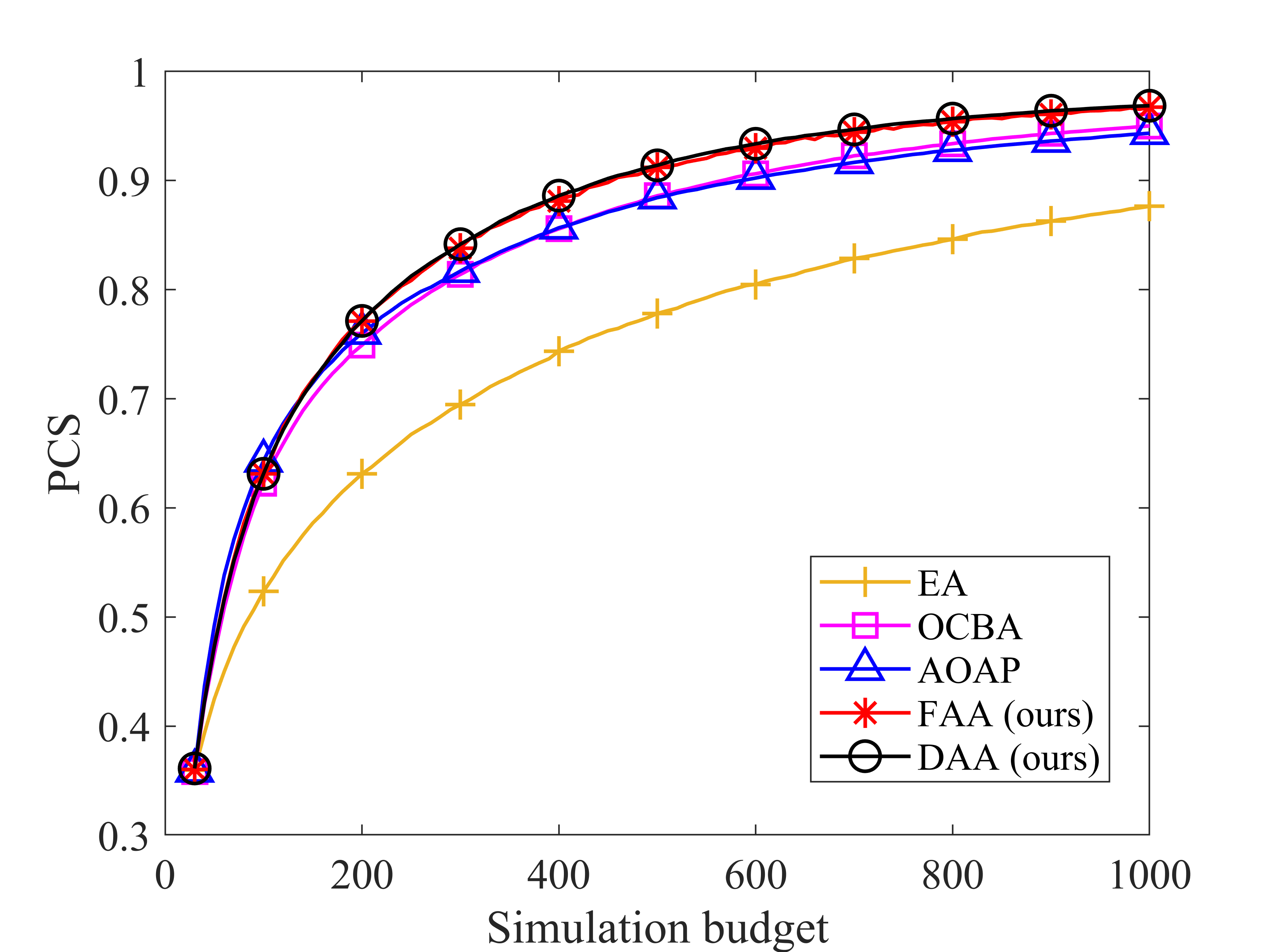
Figure 1: (Color online) Performance comparison of the five procedures on Example 1

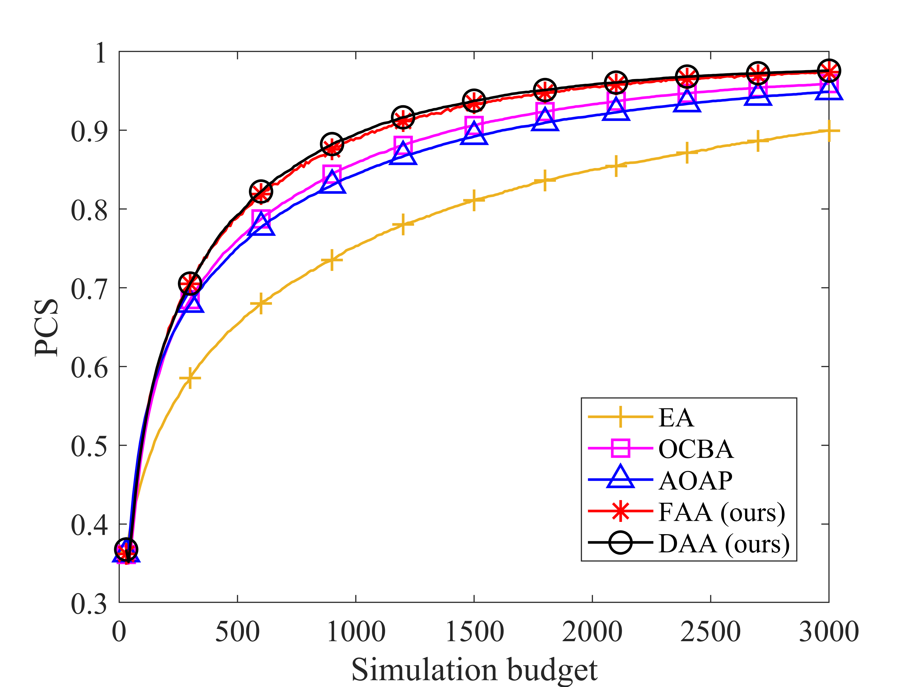
Figure 2: (Color online) Performance comparison of the five procedures on Example 2

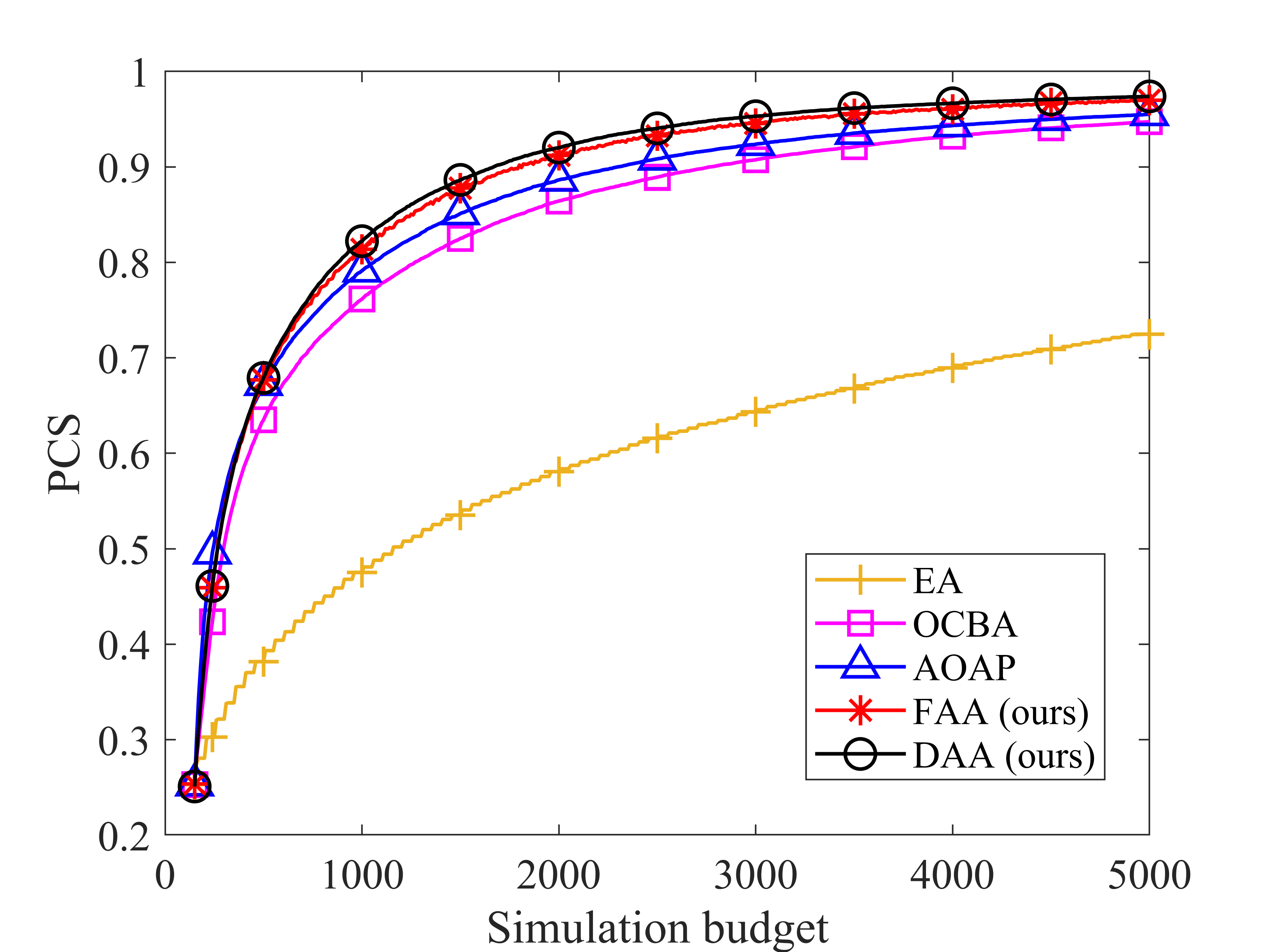
Figure 3: (Color online) Performance comparison of the five procedures on Example 3

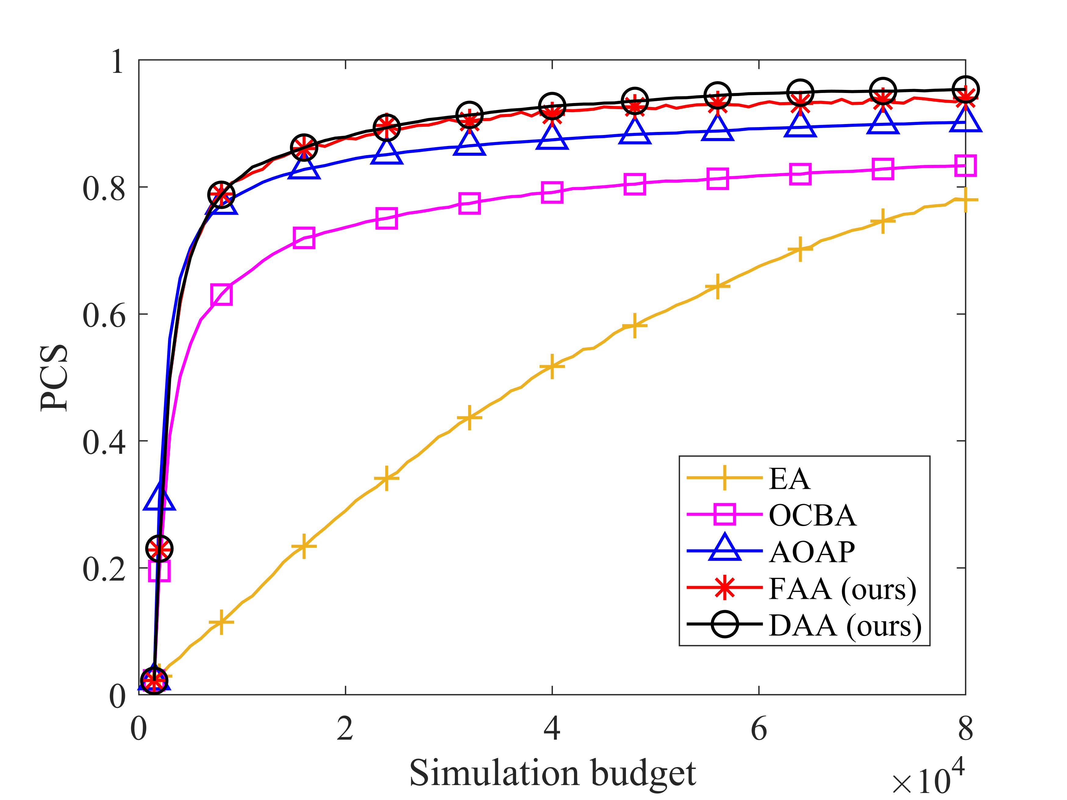
Figure 4: (Color online) Performance comparison of the five procedures on Example 4

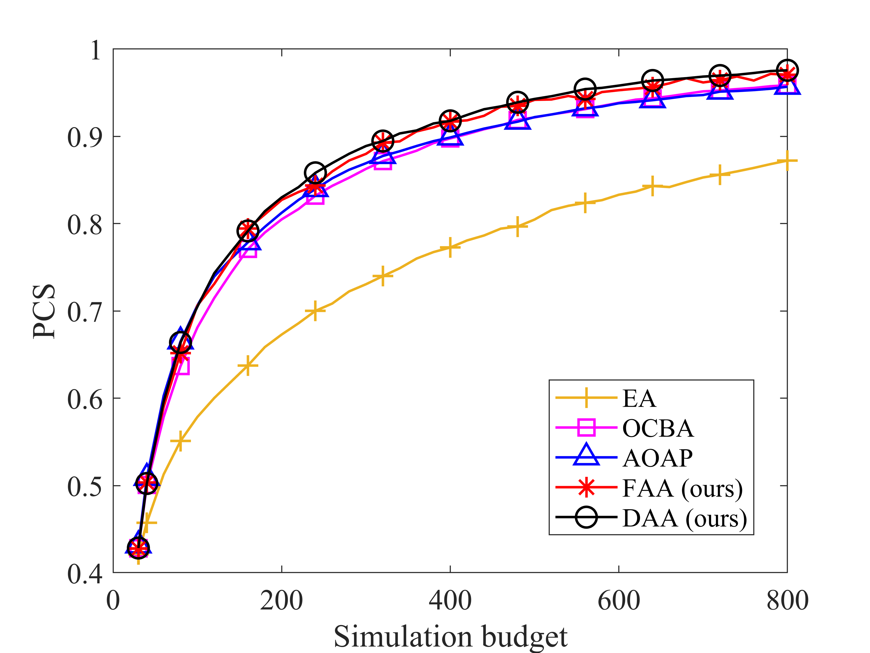
Figure 5: (Color online) Performance comparison of the five allocation procedures on the facility location problem

TABLE II: Performance comparison of the five allocation procedures on different simulation budgets for synthetic examples

Example 1	Simulation budget
	50	100	200	400	600	800	1000
EA	0.425	0.523	0.631	0.744	0.805	0.846	0.876
OCBA	0.466	0.623	0.749	0.856	0.906	0.934	0.950
AOAP	0.492	0.643	0.760	0.857	0.902	0.928	0.943
FAA (ours)	0.474	0.631	0.771	0.981	0.930	0.954	0.967
DAA (ours)	0.473	0.631	0.771	0.986	0.934	0.957	0.969
Example 2	Simulation budget
	50	150	500	1000	1500	2000	3000
EA	0.389	0.505	0.654	0.753	0.811	0.850	0.900
OCBA	0.388	0.571	0.760	0.858	0.906	0.933	0.959
AOAP	0.404	0.583	0.751	0.844	0.892	0.919	0.949
FAA (ours)	0.398	0.589	0.789	0.890	0.935	0.955	0.974
DAA (ours)	0.396	0.586	0.792	0.895	0.938	0.958	0.976
Example 3	Simulation budget
	200	500	800	1000	2000	3000	5000
EA	0.281	0.382	0.443	0.375	0.581	0.643	0.725
OCBA	0.356	0.635	0.724	0.762	0.864	0.907	0.947
AOAP	0.429	0.672	0.755	0.791	0.886	0.924	0.955
FAA (ours)	0.383	0.677	0.775	0.814	0.912	0.945	0.970
DAA (ours)	0.382	0.679	0.782	0.822	0.920	0.953	0.974
Example 4	Simulation budget ($\times 10^{3}$)
	6	8	10	20	30	60	80
EA	0.089	0.115	0.145	0.290	0.414	0.675	0.780
OCBA	0.591	0.631	0.658	0.736	0.768	0.818	0.834
AOAP	0.734	0.772	0.791	0.841	0.862	0.892	0.902
FAA (ours)	0.733	0.789	0.813	0.877	0.906	0.931	0.940
DAA (ours)	0.729	0.788	0.817	0.879	0.910	0.947	0.954
Facility location problem	Simulation budget
	40	120	200	300	500	700	800
EA	0.458	0.600	0.673	0.731	0.805	0.853	0.872
OCBA	0.501	0.715	0.805	0.863	0.922	0.952	0.959
AOAP	0.509	0.740	0.813	0.869	0.922	0.947	0.957
FAA (ours)	0.504	0.731	0.827	0.880	0.942	0.962	0.971
DAA (ours)	0.502	0.743	0.830	0.889	0.943	0.968	0.976

V-B Discussion on Experiment Results

From Figure 1-5 and Table II, we can see that both FAA and DAA have the best overall performances across all tested examples. This observation verifies the benefits of the proposed budget-adaptive allocation rule. AOAP performs the best at the beginning, but it surpassed by both FAA and DAA when the simulation budget is relatively large. This observation corresponds to the fact that AOAP is a myopic procedure that maximizes one-step-ahead improvement but can not adapt to the simulation budget. When the problem scale is small (e.g., Example 1-3 and the facility location problem), AOAP and OCBA are compatible. However, when the problem scale is relatively large (e.g., Example 4), AOAP performs better than OCBA. It is interesting to see in Example 2 that competitive designs (that are hard to distinguish from the best design) are assigned large budget allocation ratios by OCBA due to their large variances. However, based on the finite budget size, the budget allocation ratios assigned to competitive designs and non-competitive designs should be discounted and increased, respectively. Therefore, both FAA and DAA, which consider the impact of simulation budget, have better performances than OCBA on Example 2 (see Figure 2). Since EA incorporates no sample information and is a pure random sampling procedure, it is dominated by the other four procedures. The reason why both FAA and DAA have superior performances is that they consider the impact of budget size on budget allocation strategies and possess not only desirable finite-budget properties but also asymptotic optimality.

In Table II, we can see that FAA performs slightly better than DAA when the simulation budget is relatively small. This verifies the benefit of anchoring the final budget. However, FAA is outperformed by DAA after the simulation budget grows up to 400, 500, 500, 10,000, and 120 in Example 1, 2, 3, 4, and the facility location problem, respectively. These observations illustrate that, when the simulation budget $T$ or the problem scale is relatively small, FAA is preferred. Otherwise, DAA is recommended.

As shown in Table III, we can see that EA are the fastest procedure as it does not utilize any sample information. The average runtimes for both FAA and DAA are almost the same, and they are longer than EA and OCBA but on the same magnitude as OCBA. The reason why both FAA and DAA are more time-consuming than OCBA is that, at each iteration, they require additional computational time on $\alpha_{i}(T)$ to consider the impact of budget size on budget allocation ratios. Furthermore, the average runtimes of AOAP are compatible with both FAA and DAA when the problem scale is relatively small, e.g., in Example 1-2. However, as the problem scale becomes large, e.g., in Example 3-4, the average runtimes of AOAP drastically increases and is much larger than both FAA and DAA. At each iteration, AOAP requires $(k-1)^{2}$ pairwise comparisons, while both FAA and DAA require $k-1$ parwise comparisons, which is the same as OCBA. Since pairwise comparisons are very time-consuming, both FAA and DAA are more computationally efficient and are more suitable for solving large-scale problems than AOAP, even though AOAP performs better when the simulation is relatively small.

The average runtimes for the five competing procedures are very close in the experiments on the facility location problem. This result implies that in the case where the complexity of the real system is high and the simulation time of such system is relative long, the additional runtimes required for calculating $\alpha_{i}(T)$ in both FAA and DAA, as well as the computational burden caused by too many pairwise comparisons in AOAP, can be negligible. Note that the industrial systems in the real world can be much more complex than the logistic system considered in this paper. Therefore, both FAA and DAA, as well as AOAP, are competitive in real industrial applications. These results verify the effectiveness and applicability of our proposed FAA and DAA procedures.

TABLE III: Average runtime of the five allocation procedures (in seconds)

	EA	OCBA	AOAP	FAA (ours)	DAA (ours)
Example 1	0.001	0.006	0.015	0.012	0.012
Example 2	0.001	0.003	0.007	0.006	0.006
Example 3	0.005	0.030	0.335	0.057	0.058
Example 4	0.009	2.780	107.061	7.802	7.842
Facility location problem	83.344	85.332	85.377	85.440	85.347

VI Conclusion

In this paper, we consider a simulation-based R&S problem of selecting the best system design from a finite set of alternatives under a fixed budget setting. We propose a budget allocation rule that is adaptive to the simulation budget and possesses both desirable finite-budget properties and asymptotic optimality. Based on the proposed budget-adaptive allocation rule, two heuristic algorithms FAA and DAA are developed. In the numerical experiments, both FAA and DAA clearly outperform other competing procedures.

We highlight the most important implication of our contributions: simulation budget significantly impacts the budget allocation strategy, and a desirable budget allocation rule should be adaptive to the simulation budget. The proposed budget-adaptive allocation rule indicates that, compared with the asymptotically optimal OCBA allocation rule, the budget allocation ratios of non-best designs that are hard to distinguish from the best design should be discounted, while the budget allocation ratios of those that are easy to distinguish from the best should be increased. These adjustments are based on the simulation budget, which is often limited and finite. Therefore, the budget allocation strategy should be sensitive to the simulation budget, and highlights the significant difference between finite budget and sufficiently large budget allocation strategies. We believe these findings can help and motivate researchers to develop more efficient finite-budget allocation rules in future studies.

The budget allocation problem can be essentially formulated as a stochastic dynamic program (DP) problem. Both FAA and DAA are efficient procedures that can adapt to the simulation budget, but they ignore the dynamic feedback of the final step while sampling at the current step. Recently, Qin, Hong, and Fan [36] in their preliminary version of work formulate the problem as a DP and investigate a non-myopic knowledge gradient (KG) procedure, which can dynamically look multiple steps ahead and take the dynamic feedback mechanism into consideration. However, exactly solving the DP is intractable due to the extremely high computational cost caused by “curse of dimensionality”. As a result, how to derive a computationally tractable allocation rule that can incorporate the dynamic feedback mechanism, remains a critical future direction.

Appendix

VI-A Proof of Lemmas

VI-A1 Proof of Lemma 1

The constraints of Problem $\mathcal{P}1$ are all affine functions of $w_{i}$, for $i\in\mathcal{K}$. Furthermore, showing APCS is concave is equivalent to showing

$$g(w)=\sum_{i\in\mathcal{K}^{\prime}}\Phi\left(-\frac{\delta_{i,b}}{\sigma_{i,b}}\right),$$

is a convex function of $w$. To verify the convexity of $g(w)$, we need to show its Hessian matrix is positive semi-definite. The Hessian matrix for $g(w)$ is

$$\nabla^{2}g(w)=\begin{pmatrix}\frac{\partial^{2}g(w)}{\partial^{2}w_{1}}&\frac{\partial^{2}g(w)}{\partial w_{1}\partial w_{2}}&\cdots&\frac{\partial^{2}g_{(}w)}{\partial w_{1}\partial w_{k}}\\ \frac{\partial^{2}g(w)}{\partial w_{2}\partial w_{1}}&\frac{\partial^{2}g(w)}{\partial^{2}w_{2}}&\cdots&\frac{\partial^{2}g(w)}{\partial w_{2}\partial w_{k}}\\ \vdots&\vdots&\ddots&\vdots\\ \frac{\partial^{2}g(w)}{\partial w_{k}\partial w_{1}}&\frac{\partial^{2}g(w)}{\partial w_{k}\partial w_{2}}&\cdots&\frac{\partial^{2}g(w)}{\partial^{2}w_{k}}\end{pmatrix},$$

where, for $i,j\in\mathcal{K}^{\prime}$ and $i\neq j$, and $b$

$$\frac{\partial^{2}g(w)}{\partial w_{i}^{2}} =\frac{1}{2\sqrt{2\pi}}\exp\left(-\frac{\delta_{i,b}^{2}}{2\sigma_{i,b}^{2}}\right)$$

$$\quad\times\left[\frac{\delta_{i,b}}{\sigma_{i,b}^{5}T^{2}}\frac{\sigma_{i}^{4}}{w_{i}^{4}}\left(\frac{1}{2}\frac{\delta_{i,b}^{2}}{\sigma_{i,b}^{2}}-\frac{3}{2}\right)+2\frac{\delta_{i,b}}{\sigma_{i,b}^{3}T}\frac{\sigma_{i}^{2}}{w_{i}^{3}}\right],$$

$$\frac{\partial^{2}g(w)}{\partial w_{b}^{2}} =\frac{1}{2\sqrt{2\pi}}\sum\limits_{i\in\mathcal{K}^{\prime}}\exp\left(-\frac{\delta_{i,b}^{2}}{2\sigma_{i,b}^{2}}\right)$$

$$\quad\times\left[\frac{\delta_{i,b}}{\sigma_{i,b}^{5}T^{2}}\frac{\sigma_{b}^{4}}{w_{b}^{4}}\left(\frac{1}{2}\frac{\delta_{i,b}^{2}}{\sigma_{i,b}^{2}}-\frac{3}{2}\right)+2\frac{\delta_{i,b}}{\sigma_{i,b}^{3}T}\frac{\sigma_{b}^{2}}{w_{b}^{3}}\right],$$

$$\frac{\partial^{2}g(w)}{\partial w_{i}\partial w_{b}} =\frac{1}{2\sqrt{2\pi}}\exp\left(-\frac{\delta_{i,b}^{2}}{2\sigma_{i,b}^{2}}\right)$$

$$\quad\times\left[\frac{\delta_{i,b}}{\sigma_{i,b}^{5}T^{2}}\frac{\sigma_{i}^{2}}{w_{i}^{2}}\frac{\sigma_{b}^{2}}{w_{b}^{2}}\left(\frac{1}{2}\frac{\delta_{i,b}^{2}}{\sigma_{i,b}^{2}}-\frac{3}{2}\right)\right],$$

$$\frac{\partial^{2}g(w)}{\partial w_{i}\partial w_{j}} =0.$$

Furthermore, for any non-zero vector $a\in\mathbb{R}^{k}$, we have

$$a^{T}\nabla^{2}g(w)a$$

$$=\sum\limits_{i\in\mathcal{K}^{\prime}}\frac{\partial^{2}g(w)}{\partial w_{i}^{2}}a_{i}^{2}+\frac{\partial^{2}g(w)}{\partial w_{b}^{2}}a_{b}^{2}$$

$$\quad+2\sum\limits_{i\in\mathcal{K}^{\prime}}\frac{\partial^{2}g(w)}{\partial w_{i}\partial w_{b}}a_{i}a_{b}$$

$$=\frac{1}{2\sqrt{2\pi}}\sum\limits_{i\in\mathcal{K}^{\prime}}\exp\left(-\frac{\delta_{i,b}^{2}}{2\sigma_{i,b}^{2}}\right)$$

$$\quad\times a_{i}^{2}\left[\frac{\delta_{i,b}}{\sigma_{i,b}^{5}T^{2}}\frac{\sigma_{i}^{4}}{w_{i}^{4}}\left(\frac{1}{2}\frac{\delta_{i,b}^{2}}{\sigma_{i,b}^{2}}-\frac{3}{2}\right)+2\frac{\delta_{i,b}}{\sigma_{i,b}^{3}T}\frac{\sigma_{i}^{2}}{w_{i}^{3}}\right]$$

$$\quad+\frac{1}{2\sqrt{2\pi}}\sum\limits_{i\in\mathcal{K}^{\prime}}\exp\left(-\frac{\delta_{i,b}^{2}}{2\sigma_{i,b}^{2}}\right)$$

$$\quad\times a_{b}^{2}\left[\frac{\delta_{i,b}}{\sigma_{i,b}^{5}T^{2}}\frac{\sigma_{b}^{4}}{w_{b}^{4}}\left(\frac{1}{2}\frac{\delta_{i,b}^{2}}{\sigma_{i,b}^{2}}-\frac{3}{2}\right)+2\frac{\delta_{i,b}}{\sigma_{i,b}^{3}T}\frac{\sigma_{b}^{2}}{w_{b}^{3}}\right]$$

$$\quad+\frac{1}{2\sqrt{2\pi}}\sum\limits_{i\in\mathcal{K}^{\prime}}\exp\left(-\frac{\delta_{i,b}^{2}}{2\sigma_{i,b}^{2}}\right)$$

$$\quad\times 2a_{i}a_{b}\left[\frac{\delta_{i,b}}{\sigma_{i,b}^{5}T^{2}}\frac{\sigma_{i}^{2}}{w_{i}^{2}}\frac{\sigma_{b}^{2}}{w_{b}^{2}}\left(\frac{1}{2}\frac{\delta_{i,b}^{2}}{\sigma_{i,b}^{2}}-\frac{3}{2}\right)\right]$$

$$=\frac{1}{2\sqrt{2\pi}}\sum\limits_{i\in\mathcal{K}^{\prime}}\exp\left(-\frac{\delta_{i,b}^{2}}{2\sigma_{i,b}^{2}}\right)$$

$$\quad\times\frac{\delta_{i,b}}{\sigma_{i,b}^{3}T}\left[\frac{1}{\sigma_{i,b}^{2}T}\left(\frac{1}{2}\frac{\delta_{i,b}^{2}}{\sigma_{i,b}^{2}}-\frac{3}{2}\right)\left(\frac{\sigma_{i}^{2}}{w_{i}^{2}}a_{i}+\frac{\sigma_{b}^{2}}{w_{b}^{2}}a_{b}\right)^{2}\right.$$

$$\left.\quad\quad+2\left(\frac{\sigma_{i}^{2}}{w_{i}^{3}}a_{i}^{2}+\frac{\sigma_{b}^{2}}{w_{b}^{3}}a_{b}^{2}\right)\right].$$

Since

$$2\left(\frac{\sigma_{i}^{2}}{w_{i}^{3}}a_{i}^{2}+\frac{\sigma_{b}^{2}}{w_{b}^{3}}a_{b}^{2}\right) =2\frac{\sigma_{i,b}^{2}}{\sigma_{i,b}^{2}}\left(\frac{\sigma_{i}^{2}}{w_{i}^{3}}a_{i}^{2}+\frac{\sigma_{b}^{2}}{w_{b}^{3}}a_{b}^{2}\right)$$

$$=\frac{2}{\sigma_{i,b}^{2}T}\left(\frac{\sigma_{i}^{2}}{w_{i}}+\frac{\sigma_{b}^{2}}{w_{b}}\right)\left(\frac{\sigma_{i}^{2}}{w_{i}^{3}}a_{i}^{2}+\frac{\sigma_{b}^{2}}{w_{b}^{3}}a_{b}^{2}\right)$$

$$=\frac{2}{\sigma_{i,b}^{2}T}\left[\left(\frac{\sigma_{i}^{2}}{w_{i}^{2}}a_{i}+\frac{\sigma_{b}^{2}}{w_{b}^{2}}a_{b}\right)^{2}\right.$$

$$\left.\quad\quad+\frac{\sigma_{i}^{2}\sigma_{b}^{2}}{w_{i}w_{b}}\left(\frac{a_{i}}{w_{i}}-\frac{a_{b}}{w_{b}}\right)^{2}\right],$$

we have

$$\frac{1}{\sigma_{i,b}^{2}T}\left(\frac{1}{2}\frac{\delta_{i,b}^{2}}{\sigma_{i,b}^{2}}-\frac{3}{2}\right)\left(\frac{\sigma_{i}^{2}}{w_{i}^{2}}a_{i}+\frac{\sigma_{b}^{2}}{w_{b}^{2}}a_{b}\right)^{2}$$

$$\quad+2\left(\frac{\sigma_{i}^{2}}{w_{i}^{3}}a_{i}^{2}+\frac{\sigma_{b}^{2}}{w_{b}^{3}}a_{b}^{2}\right)$$

$$= \frac{1}{\sigma_{i,b}^{2}T}\left[\left(\frac{1}{2}\frac{\delta_{i,b}^{2}}{\sigma_{i,b}^{2}}-\frac{3}{2}\right)\left(\frac{\sigma_{i}^{2}}{w_{i}^{2}}a_{i}+\frac{\sigma_{b}^{2}}{w_{b}^{2}}a_{b}\right)^{2}\right.$$

$$\left.\quad+2\left(\frac{\sigma_{i}^{2}}{w_{i}^{2}}a_{i}+\frac{\sigma_{b}^{2}}{w_{b}^{2}}a_{b}\right)^{2}+2\frac{\sigma_{i}^{2}\sigma_{b}^{2}}{w_{i}w_{b}}\left(\frac{a_{i}}{w_{i}}-\frac{a_{b}}{w_{b}}\right)^{2}\right]$$

$$= \frac{1}{\sigma_{i,b}^{2}T}\left[\left(\frac{1}{2}\frac{\delta_{i,b}^{2}}{\sigma_{i,b}^{2}}+\frac{1}{2}\right)\left(\frac{\sigma_{i}^{2}}{w_{i}^{2}}a_{i}+\frac{\sigma_{b}^{2}}{w_{b}^{2}}a_{b}\right)^{2}\right.$$

$$\left.\quad+2\frac{\sigma_{i}^{2}\sigma_{b}^{2}}{w_{i}w_{b}}\left(\frac{a_{i}}{w_{i}}-\frac{a_{b}}{w_{b}}\right)^{2}\right]$$

$$\geq 0,$$

and therefore, $\nabla^{2}g(w)\succeq 0$, and $g(w)$ is a convex function of $w$. Due to the two constraints $\sum_{i\in\mathcal{K}}w_{i}=1$ and $w_{i}\geq 0$, for $i\in\mathcal{K}$, forming a convex set, Problem $\mathcal{P}1$ is a convex optimization problem. This result concludes the proof.

VI-A2 Proof of Lemma 2

By condition $\widehat{\mathcal{C}}_{2}$, for $i\in\mathcal{K}^{\prime}$, we have

$$\begin{split}w_{i}&=\frac{\lambda-2\log I_{i}}{\frac{T}{I_{i}}+\frac{1}{w^{*}_{i}}}\\ &=\frac{I_{i}(\lambda-2\log I_{i})}{T+S},\end{split}$$ (14)

in which, $S=\sum_{i\in\mathcal{K}}I_{i}$ and $w^{*}_{i}=I_{i}/S$. We substitute $w_{i}$ provided by (14) into condition $\mathcal{C}_{1}$, and obtain

$$w_{b}=\sigma_{b}\sqrt{\sum\limits_{i\in\mathcal{K}^{\prime}}\frac{I_{i}^{2}(\lambda-2\log I_{i})^{2}}{\sigma_{i}^{2}(T+S)^{2}}}.$$ (15)

For $i\in\mathcal{K}^{\prime}$, by condition $\mathcal{C}_{3}$, (14), and (15)

$$\sum\limits_{i\in\mathcal{K}^{\prime}}\frac{I_{i}(\lambda-2\log I_{i})}{T+S}+\sigma_{b}\sqrt{\sum\limits_{i\in\mathcal{K}^{\prime}}\frac{I_{i}^{2}(\lambda-2\log I_{i})^{2}}{\sigma_{i}^{2}\left(T+S\right)^{2}}}=1.$$ (16)

Then, we have

$$\lambda=\left\{\begin{array}[]{ll}\frac{-q+\sqrt{q^{2}-4pr}}{2p}&\quad\text{if}\ w^{*}_{b}\neq\frac{1}{2}\\ \frac{4\sum_{i\in\mathcal{K}^{\prime}}I_{i}\log I_{i}+T+S}{2\sum_{i\in\mathcal{K}^{\prime}}I_{i}}&\quad\text{if}\ w^{*}_{b}=\frac{1}{2}\\ \end{array}\right.$$

where

$$\begin{split}p&=S(2I_{b}-S),\\ q&=-4\sigma_{b}^{2}\sum\limits_{i\in\mathcal{K}^{\prime}}\frac{I_{i}^{2}\log I_{i}}{\sigma_{i}^{2}}\\ &\quad\quad+2(S-I_{b})\left(2\sum\limits_{i\in\mathcal{K}^{\prime}}I_{i}\log I_{i}+T+S\right),\\ r&=4\sigma_{b}^{2}\sum\limits_{i\in\mathcal{K}^{\prime}}\frac{I_{i}^{2}\log^{2}I_{i}}{\sigma_{i}^{2}}-\left(2\sum\limits_{i\in\mathcal{K}^{\prime}}I_{i}\log I_{i}+T+S\right)^{2}.\end{split}$$

Let $\alpha_{i}(T)=\frac{(\lambda-2\log I_{i})}{1+T/S}$, for $i\in\mathcal{K}^{\prime}$, and substituting $\alpha_{i}(T)$ into (14). Then, Lemma 2 is proved.

VI-A3 Proof of Lemma 3

We now consider condition $\mathcal{C}_{4}$. For the best design $b$, its budget allocation ratio $W_{b}(T)$ is always non-negative. As for non-best designs $i\in\mathcal{K}^{\prime}$, let $W_{i}(T)\geq 0$, and we have

$$\lambda \geq 2\log I_{i}\quad\forall i\in\mathcal{K}^{\prime},$$

$$\geq 2\log I_{\langle k-1\rangle}.$$

If $w^{*}_{b}=1/2$

$$\lambda=\frac{4\sum_{i\in\mathcal{K}^{\prime}}I_{i}\log I_{i}+T+S}{2\sum_{i\in\mathcal{K}^{\prime}}I_{i}}\geq 2\log I_{\langle k-1\rangle},$$

and it can be checked that $T\geq 4\sum_{i\in\mathcal{K}^{\prime}}I_{i}\log(I_{\langle k-1\rangle}/I_{i})-S$.

If $w^{*}_{b}\neq 1/2$

$$\lambda=\frac{-q+\sqrt{q^{2}-4pr}}{2p}\geq 2\log I_{\langle k-1\rangle},$$

where $p$, $q$, and $r$ are given in Lemma 2.

Case 1: If $p=2w_{b}^{*}-1>0$, i.e. $w_{b}^{*}>1/2$, we need to solve the following inequality

$$\sqrt{q^{2}-4pr}\geq 4p\log I_{\langle k-1\rangle}+q.$$ (17)

Additionally

$$\begin{split}&4p\log I_{\langle k-1\rangle}+q\\ =&4\sum\limits_{i\in\mathcal{K}^{\prime}}\left(\frac{\sigma^{2}_{b}(w_{i}^{*})^{2}}{\sigma_{i}^{2}}-(1-w_{b}^{*})w_{i}^{*}\right)\log\frac{I_{\langle k-1\rangle}}{I_{i}}\\ &\quad+2(1-w_{b}^{*})\frac{T+S}{S}.\\ \end{split}$$

Furthermore, we define

$$T_{1}=2\sum\limits_{i\in\mathcal{K}^{\prime}}\left[\frac{\sigma^{2}_{b}I_{i}^{2}}{\sigma_{i}^{2}(S-I_{b})}-I_{i}\right]\log\frac{I_{\langle k-1\rangle}}{I_{i}}-S.$$

When $T<T_{1}$, $4p\log I_{\langle k-1\rangle}+q<0$, then Inequality (17) always holds. Otherwise, when $T\geq T_{1}$, we take square on both sides of (17) and obtain

$$T\in(-\infty,T_{3}]\cup[T_{2},+\infty),$$

in which

$$\begin{split}T_{2}&=2\left[\sum\limits_{i\in\mathcal{K}^{\prime}}I_{i}\log\frac{I_{\langle k-1\rangle}}{I_{i}}\right.\\ &\left.\quad\quad+\sigma_{b}\sqrt{\sum\limits_{i\in\mathcal{K}^{\prime}}\frac{I_{i}^{2}}{\sigma_{i}^{2}}\left(\log\frac{I_{\langle k-1\rangle}}{I_{i}}\right)^{2}}\right]-S,\\ T_{3}&=2\left[\sum\limits_{i\in\mathcal{K}^{\prime}}I_{i}\log\frac{I_{\langle k-1\rangle}}{I_{i}}\right.\\ &\left.\quad\quad-\sigma_{b}\sqrt{\sum\limits_{i\in\mathcal{K}^{\prime}}\frac{I_{i}^{2}}{\sigma_{i}^{2}}\left(\log\frac{I_{\langle k-1\rangle}}{I_{i}}\right)^{2}}\right]-S.\\ \end{split}$$

It can be checked that $T_{2}$ is strictly positive. Due to the fact $\lim_{T\rightarrow\infty}W_{i}(T)\rightarrow w_{i}^{*}\geq 0$, for $i\in\mathcal{K}^{\prime}$, we expect that $T$ can be sufficiently large. Therefore, a sufficient condition for $W(T)$ being feasible, when $w_{b}^{*}>1/2$, is $T\geq\max\{T_{1},T_{2}\}$.

Case 2: If $p=2w_{b}^{*}-1<0$, i.e. $w_{b}^{*}<1/2$, similarly, we need to solve the following inequality

$$\sqrt{q^{2}-4pr}\leq 4p\log I_{\langle k-1\rangle}+q.$$ (18)

When $T<T_{1}$, Inequality (18) never holds. Otherwise, we take square on both sides of (18) and, similarly, obtain $T\in(-\infty,T_{3}]\cup[T_{2},+\infty)$. Therefore, a sufficient condition for $W(T)$ being feasible, when $w_{b}^{*}<1/2$, is $T\geq\max\{T_{1},T_{2}\}$.

Hence, the solution $W(T)$ is always feasible if $T\geq T_{0}$, where

$$T_{0}=\left\{\begin{array}[]{ll}\max\{T_{1},T_{2}\}&\quad\text{if}\ w^{*}_{b}\neq\frac{1}{2}\\ 4\sum_{i\in\mathcal{K}^{\prime}}I_{i}\log\frac{I_{\langle k-1\rangle}}{I_{i}}-S&\quad\text{if}\ w^{*}_{b}=\frac{1}{2}\\ \end{array}\right.$$

These results conclude the proof.

VI-B Proof of Theorems

VI-B1 Proof of Theorem 1

Let $\lambda$ and $\nu_{i}$, for $i\in\mathcal{K}$, be the Lagrange multipliers. The KKT conditions for Problem $\mathcal{P}1$ are as follows

$$-\frac{1}{2\sqrt{2\pi}}\exp\left(-\frac{\delta_{i,b}^{2}}{2\sigma_{i,b}^{2}}\right)\frac{\delta_{i,b}}{\sigma_{i,b}^{3}}\frac{\sigma_{i}^{2}}{Tw_{i}^{2}}-\lambda-\nu_{i}=0,\ i\in\mathcal{K}^{\prime},$$ (19)

$$-\frac{1}{2\sqrt{2\pi}}\frac{\sigma_{b}^{2}}{Tw_{b}^{2}}\left[\sum_{i\in\mathcal{K}^{\prime}}\exp\left(-\frac{\delta_{i,b}^{2}}{2\sigma_{i,b}^{2}}\right)\frac{\delta_{i,b}}{\sigma_{i,b}^{3}}\right]-\lambda-\nu_{b}=0,$$ (20)

$$\nu_{i}w_{i}=0,\quad i\in\mathcal{K},$$ (21)

$$\sum\limits_{i\in\mathcal{K}}w_{i}=1,$$ (22)

$$w_{i}\geq 0,\quad i\in\mathcal{K}.$$ (23)

Assuming $w_{i}$ is strictly positive, thus we have $\nu_{i}=0$, for $i\in\mathcal{K}$. Condition $\mathcal{C}_{1}$ can be derived by substituting (19) into (20). Take logarithm on both sides of (19), then condition $\mathcal{C}_{2}$ follows. Equations (22) and (23) are conditions $\mathcal{C}_{3}$ and $\mathcal{C}_{4}$, respectively, both of which guarantee the feasibility of Problem $\mathcal{P}1$.

VI-C Proof of Propositions

VI-C1 Proof of Proposition 1

We first show that for any pair of non-best designs $i,j\in\mathcal{K}^{\prime}$ and $i\neq j$, there exists a positive constant $c_{i,j}>0$ such that $w_{i}/w_{j}\leq c_{i,j}$. We prove this by contradiction. Assume that there exists a pair of designs $i,j\in\mathcal{K}^{\prime}$ and $i\neq j$ such that $w_{i}/w_{j}$ can not be upper bounded, i.e., $w_{i}/w_{j}=\infty$. Since $w_{i},w_{j}\in[0,1]$, it can be checked that $w_{j}\rightarrow 0$. By condition $\mathcal{C}_{2}$ in Theorem 1

$$\begin{split}&\left[\frac{\delta_{j,b}^{2}}{(\sigma_{j}^{2}/w_{j}+\sigma_{b}^{2}/w_{b})}-\frac{\delta_{i,b}^{2}}{(\sigma_{i}^{2}/w_{i}+\sigma_{b}^{2}/w_{b})}\right]\frac{T}{2}\\ &\quad\quad=\log\frac{\delta_{j,b}(\sigma_{j}^{2}/w^{2}_{j})(\sigma_{i}^{2}/w_{i}+\sigma_{b}^{2}/w_{b})^{\frac{3}{2}}}{\delta_{i,b}(\sigma_{i}^{2}/w^{2}_{i})(\sigma_{j}^{2}/w_{j}+\sigma_{b}^{2}/w_{b})^{\frac{3}{2}}}.\end{split}$$ (24)

As $w_{j}\rightarrow 0$, the term $\frac{\delta_{j,b}^{2}}{(\sigma_{j}^{2}/w_{j}+\sigma_{b}^{2}/w_{b})}$ in (24) will vanish, and the right-hand side in (24) will approach infinity. Then, as $w_{j}\rightarrow 0$, we have

$$-\frac{\delta_{i,b}^{2}}{2(\sigma_{i}^{2}/w_{i}+\sigma_{b}^{2}/w_{b})}T=+\infty,$$

which is true if $\sigma_{i}^{2}/w_{i}+\sigma_{b}^{2}/w_{b}\rightarrow 0^{-}$. However, this contradicts with the fact $\sigma_{i}^{2}/w_{i}+\sigma_{b}^{2}/w_{b}>0$. Thus, the assumption is false, and for any pair of designs $i,j\in\mathcal{K}^{\prime}$ and $i\neq j$, there must exist a positive constant $c_{i,j}>0$, such that $w_{i}/w_{j}\leq c_{i,j}$.

Let $w_{\text{min}}$ be the minimum budget allocation ratio of non-best designs, i.e., $w_{\text{min}}=\min_{i\in\mathcal{K}^{\prime}}w_{i}$. Therefore, there exists a positive constant $c$ such that $w_{i}\leq cw_{\text{min}}$, for $i\in\mathcal{K}^{\prime}$. By condition $\mathcal{C}_{1}$ in Theorem 1

$$w_{b}=\sigma_{b}\sqrt{\sum\limits_{i\in\mathcal{K}^{\prime}}\frac{w_{i}^{2}}{\sigma_{i}^{2}}}\geq\frac{\sigma_{b}\sqrt{k-1}}{\bar{\sigma}}w_{\text{min}}.$$

Then, for any non-best design $i\in\mathcal{K}^{\prime}$, we have

$$\frac{w_{i}}{w_{b}}\leq\frac{w_{i}}{w_{\text{min}}}\frac{\bar{\sigma}}{\sigma_{b}\sqrt{k-1}}\leq\frac{\bar{\sigma}}{\underline{\sigma}}\frac{c}{\sqrt{k-1}}.$$

This result concludes the proof, and therefore, $w_{i}/w_{b}=\mathcal{O}(1/\sqrt{k})$, for $i\in\mathcal{K}^{\prime}$.

VI-C2 Proof of Proposition 2

According to Lemma 2, we have

$$\alpha_{i}(T)=\frac{(\lambda-2\log I_{i})}{1+T/S},\quad i\in\mathcal{K}^{\prime},$$

which is monotone decreasing with respect to $I_{i}$. Since $I_{\langle 1\rangle}\leq I_{\langle 2\rangle}\leq\dots\leq I_{\langle k-1\rangle}$, we have $\alpha_{\langle 1\rangle}(T)\geq\alpha_{\langle 2\rangle}(T)\geq\dots\geq\alpha_{\langle k-1\rangle}(T)$. Furthermore, if $I_{i}$, for $i\in\mathcal{K}^{\prime}$, are all equal, then $\lambda=1+T/S+2\log I_{i}$ and $\alpha_{\langle 1\rangle}(T)=\alpha_{\langle 2\rangle}^{(}T)=\dots=\alpha_{\langle k-1\rangle}(T)=1$. On the contrary, if $\alpha_{\langle 1\rangle}(T)=\alpha_{\langle 2\rangle}(T)=\dots=\alpha_{\langle k-1\rangle}(T)$, it can be checked that all $I_{i}$s are equal.

We show $\alpha_{\langle 1\rangle}(T)\geq 1$ by contradiction, and $\alpha_{\langle k-1\rangle}(T)\leq 1$ can be proved similarly. Without lose of generality, we assume $\alpha_{\langle 1\rangle}(T)<1$. Based on preceding analyses, we know $\alpha_{\langle k-1\rangle}(T)\leq\alpha_{[k-2]}(T)\leq\dots\leq\alpha_{\langle 1\rangle}(T)<1$. According to Lemma 2, we have $W_{i}(T)=w^{*}_{i}\alpha_{i}(T)<w^{*}_{i}$ for non-best designs $i\in\mathcal{K}^{\prime}$, and $W_{b}(T)=\sigma_{b}\sqrt{\sum_{i\in\mathcal{K}^{\prime}}\frac{(w_{i}^{*}\alpha_{i}(T))^{2}}{\sigma_{i}^{2}}}<w^{*}_{b}$ for the best design $b$. Then we have $\sum_{i\in\mathcal{K}}W_{b}(T)<\sum_{i\in\mathcal{K}}w^{*}_{b}=1$, which contradicts with the fact $\sum_{i\in\mathcal{K}}W_{b}(T)=1$. Therefore, $\alpha_{\langle 1\rangle}(T)$ must be larger or equal to 1. These results conclude the proof.

References

References

- [1] B. P. Zeigler, H. Praehofer, and T. G. Kim, Theory of modeling and simulation. Academic press, 2000.
- [2] J. Banks, Discrete event system simulation. Pearson Education India, 2005.
- [3] S.-H. Kim and B. L. Nelson, “Selecting the best system,” Handbooks in operations research and management science, vol. 13, pp. 501–534, 2006.
- [4] C.-H. Chen and L. H. Lee, Stochastic simulation optimization: an optimal computing budget allocation. World scientific, 2011, vol. 1.
- [5] C. Fu, C. Fu, and M. Michael, Handbook of simulation optimization. Springer, 2015.
- [6] Y.-C. Ho, R. Sreenivas, and P. Vakili, “Ordinal optimization of deds,” Discrete Event Dyn. Syst., vol. 2, no. 1, pp. 61–88, 1992.
- [7] Y.-C. Ho, Q.-C. Zhao, and Q.-S. Jia, Ordinal optimization: Soft optimization for hard problems. Springer Science & Business Media, 2008.
- [8] C.-H. Chen, J. Lin, E. Yücesan, and S. E. Chick, “Simulation budget allocation for further enhancing the efficiency of ordinal optimization,” Discrete Event Dyn. Syst., vol. 10, no. 3, pp. 251–270, 2000.
- [9] Y. Peng, C.-H. Chen, M. C. Fu, and J.-Q. Hu, “Non-monotonicity of probability of correct selection,” in Proc. Winter Simul. Conf., 2015, pp. 3678–3689.
- [10] ——, “Gradient-based myopic allocation policy: An efficient sampling procedure in a low-confidence scenario,” IEEE Trans. Autom. Control, vol. 63, no. 9, pp. 3091–3097, 2017.
- [11] S. E. Chick, J. Branke, and C. Schmidt, “Sequential sampling to myopically maximize the expected value of information,” INFORMS J. Comput., vol. 22, no. 1, pp. 71–80, 2010.
- [12] P. I. Frazier, W. B. Powell, and S. Dayanik, “A knowledge-gradient policy for sequential information collection,” SIAM J. Control Optim., vol. 47, no. 5, pp. 2410–2439, 2008.
- [13] Z. Shi, Y. Peng, L. Shi, C.-H. Chen, and M. C. Fu, “Dynamic sampling allocation under finite simulation budget for feasibility determination,” INFORMS J. Comput., vol. 34, no. 1, pp. 557–568, 2022.
- [14] S.-H. Kim and B. L. Nelson, “A fully sequential procedure for indifference-zone selection in simulation,” ACM Trans. Model. Comput. Simul., vol. 11, no. 3, pp. 251–273, 2001.
- [15] L. J. Hong and B. L. Nelson, “The tradeoff between sampling and switching: New sequential procedures for indifference-zone selection,” IIE Trans., vol. 37, no. 7, pp. 623–634, 2005.
- [16] D. Batur and S.-H. Kim, “Fully sequential selection procedures with a parabolic boundary,” IIE Trans., vol. 38, no. 9, pp. 749–764, 2006.
- [17] L. J. Hong and B. L. Nelson, “Selecting the best system when systems are revealed sequentially,” IIE Trans., vol. 39, no. 7, pp. 723–734, 2007.
- [18] W. Fan, L. J. Hong, and B. L. Nelson, “Indifference-zone-free selection of the best,” Oper. Res., vol. 64, no. 6, pp. 1499–1514, 2016.
- [19] J. Luo, L. J. Hong, B. L. Nelson, and Y. Wu, “Fully sequential procedures for large-scale ranking-and-selection problems in parallel computing environments,” Oper. Res., vol. 63, no. 5, pp. 1177–1194, 2015.
- [20] Y. Zhong and L. J. Hong, “Knockout-tournament procedures for large-scale ranking and selection in parallel computing environments,” Oper. Res., vol. 70, no. 1, pp. 432–453, 2022.
- [21] L. J. Hong, G. Jiang, and Y. Zhong, “Solving large-scale fixed-budget ranking and selection problems,” INFORMS J. Comput., vol. 34, no. 6, pp. 2930–2949, 2022.
- [22] P. Glynn and S. Juneja, “A large deviations perspective on ordinal optimization,” in Proc. Winter Simul. Conf., vol. 1, 2004.
- [23] S. Gao and W. Chen, “A new budget allocation framework for selecting top simulated designs,” IIE Trans., vol. 48, no. 9, pp. 855–863, 2016.
- [24] Y. Peng and M. C. Fu, “Myopic allocation policy with asymptotically optimal sampling rate,” IEEE Trans. Autom. Control, vol. 62, no. 4, pp. 2041–2047, 2016.
- [25] Y. Peng, E. K. Chong, C.-H. Chen, and M. C. Fu, “Ranking and selection as stochastic control,” IEEE Trans. Autom. Control, vol. 63, no. 8, pp. 2359–2373, 2018.
- [26] Y. Peng, C.-H. Chen, M. C. Fu, and J.-Q. Hu, “Dynamic sampling allocation and design selection,” INFORMS J. Comput., vol. 28, no. 2, pp. 195–208, 2016.
- [27] C.-H. Chen, D. He, M. Fu, and L. H. Lee, “Efficient simulation budget allocation for selecting an optimal subset,” INFORMS J. Comput., vol. 20, no. 4, pp. 579–595, 2008.
- [28] S. Zhang, L. H. Lee, E. P. Chew, J. Xu, and C.-H. Chen, “A simulation budget allocation procedure for enhancing the efficiency of optimal subset selection,” IEEE Trans. Autom. Control, vol. 61, no. 1, pp. 62–75, 2015.
- [29] G. Zhang, B. Chen, Q.-S. Jia, and Y. Peng, “Efficient sampling policy for selecting a subset with the best,” IEEE Trans. Autom. Control, 2022.
- [30] S. Gao, H. Xiao, E. Zhou, and W. Chen, “Robust ranking and selection with optimal computing budget allocation,” Automatica, vol. 81, pp. 30–36, 2017.
- [31] H. Xiao and S. Gao, “Simulation budget allocation for selecting the top-m designs with input uncertainty,” IEEE Trans. Autom. Control, vol. 63, no. 9, pp. 3127–3134, 2018.
- [32] L. H. Lee, E. P. Chew, S. Teng, and D. Goldsman, “Finding the non-dominated pareto set for multi-objective simulation models,” IIE Trans., vol. 42, no. 9, pp. 656–674, 2010.
- [33] S. R. Hunter and R. Pasupathy, “Optimal sampling laws for stochastically constrained simulation optimization on finite sets,” INFORMS J. Comput., vol. 25, no. 3, pp. 527–542, 2013.
- [34] R. Pasupathy, S. R. Hunter, N. A. Pujowidianto, L. H. Lee, and C.-H. Chen, “Stochastically constrained ranking and selection via score,” ACM Trans. Model. Comput. Simul., vol. 25, no. 1, pp. 1–26, 2014.
- [35] H. Li, H. Lam, and Y. Peng, “Efficient learning for clustering and optimizing context-dependent designs,” Oper. Res., 2022.
- [36] K. Qin, L. J. Hong, and W. Fan, “Non-myopic knowledge gradient policy for ranking and selection,” in Proc. Winter Simul. Conf., 2022, pp. 3051–3062.
- [37] S. Boyd, S. P. Boyd, and L. Vandenberghe, Convex optimization. Cambridge university press, 2004.
- [38] C.-H. Chen, “A lower bound for the correct subset-selection probability and its application to discrete-event system simulations,” IEEE Trans. Autom. Control, vol. 41, no. 8, pp. 1227–1231, 1996.
- [39] S. E. Chick and K. Inoue, “New two-stage and sequential procedures for selecting the best simulated system,” Oper. Res., vol. 49, no. 5, pp. 732–743, 2001.