Modeling still matters: a surprising instance of catastrophic floating point errors in mathematical biology and numerical methods for ODEs

Abstract

We guide the reader on a journey through mathematical modeling and numerical analysis, emphasizing the crucial interplay of both disciplines. Targeting undergraduate students with basic knowledge in dynamical systems and numerical methods for ordinary differential equations, we explore a model from mathematical biology where numerical methods fail badly due to catastrophic floating point errors. We analyze the reasons for this behavior by studying the steady states of the model and use the theory of invariants to develop an alternative model that is suited for numerical simulations. Our story intends to motivate combining analytical and numerical knowledge, even in cases where the world looks fine at first sight. We have set up an online repository containing an interactive notebook with all numerical experiments to make this study fully reproducible and useful for classroom teaching.

AMS subject classification. 37M05, 65L06, 65L20, 65P40, 97D40

1 Introduction

Setting up a nice mathematical model for some applications, using a proper numerical scheme for solving the differential equations — and wondering what is happening? Oftentimes, mathematical models of ordinary differential equations (ODEs) are easily solvable numerically as long as a suitable scheme is used. In this report, we tell a different story, which highlights the process of setting up a model and analyzing it properly for ensuring trustable and correct numerical solutions.

This article intends to take the reader on a small journey through the interplay between modeling, numerical simulation and analysis. We will pass a biological motivation on the inheritance of genes and set up a mathematical model of ODEs. As a next step, we try to get a first impression of the system’s behavior by running numerical simulations. The first plot twist is on the goodwill and trust concerning numerical simulation, even when the schemes are chosen wisely. A dynamical system analysis enlightens our misleading: By analyzing the steady states of the dynamical system, we discover the reasons for the strange simulations. The curtains fall for the theory of invariants. The friendly-looking model for inheritance turns out to conserve an important quantity — the total population — as a second integral. Accumulating floating point errors reveal the instability of steady states. By changing the system, we turn the total population into a first integral. The new model reacts in a stable way to floating point errors and trust in numerical simulations is restored.

Please use our story to motivate combining analytical and numerical knowledge, even in cases where the world looks fine at first sight. A related story focusing on step size control of numerical ODE solvers is published by Skufca [24], which we used as an inspiration for the title of this report. To make this study fully reproducible, we have set up an online repository [20] containing an interactive notebook with all numerical experiments using the modern programming language Julia.

Before starting our journey, we would like to highlight the aim of this article. The intention is not to provide new mathematical results but to motivate students from a modeling perspective why a deeper dive into mathematical analysis is helpful and provides much insight. Therefore, we refer to analytical results rather from a modeling perspective emphasizing the nature of the problems, and we include references for further studies in the end. The outlook will include literature on the theory of ordinary differential equations on manifolds with local coordinates and numerical correction schemes, further modeling examples, and structure-preserving numerical methods. During the story, the focus will be on the applied modeling perspective.

2 Modeling the inheritance of genes

Mathematical biologists strive for explaining life in mathematical terms by abstracting from individuals and finding general insight into complex processes. One big question of life is the inheritance of genes and therefore the evolution of populations. Here, we model how genes are passed on from a parent generation to the next generation. While reading, you can have in mind flowers with different possible colors or the human, or any example where two copies of a gene are present. Such an organism is called diploid. Different versions of a gene are called alleles. We consider here two different alleles, either $X$ or $x$. Possible combinations give the genotypes $XX$, $Xx$ and $xx$. If every parent inherits one of its alleles, the genotypes of the next generation are given according to the probabilities of the alleles in the parent generation. The formulation of generations implies a discrete time. In this setting, we assume all processes to be time continuous with blurred generations.

In a mathematical model, the population is divided into compartments $c_{i}$ according to their genotypes. Let $c_{1}$ be the compartment of the genotype $XX$, $c_{2}$ the compartment for the mixed genotype $Xx$, and $c_{3}$ the compartment of $xx$. The size of each compartment is time-depending.

The inheritance of the genotypes is given by Mendel’s Law of Segregation in Table 1. The genotypes of the outcomes depend on the genotypes of the parents’ generation: Every parent inherits one of its alleles, e.g. an outcome has the genotype $c_{1}$ if parents with $XX$ alleles or $Xx$ alleles mix. The probabilities of passing on the genotypes are given in Table 1.

Table 1: Mendel’s Law of Segregation: Probability of the genotypes of the outcomes.

	$c_{1}\ XX$	$c_{2}\ Xx$	$c_{3}\ xx$
$c_{1}\ XX$	1 $c_{1}$	1/2 $c_{1}$, 1/2 $c_{2}$	1 $c_{2}$
$c_{2}\ Xx$	1/2 $c_{1}$, 1/2 $c_{2}$	1/4 $c_{1}$, 1/2 $c_{2}$, 1/4 $c_{3}$	1/2 $c_{2}$, 1/2 $c_{3}$
$c_{3}\ xx$	1 $c_{2}$	1/2 $c_{2}$, 1/2 $c_{3}$	1 $c_{2}$

Following these mixing rules, Mendel’s Law of Segregation can be transformed into ordinary differential equations for the genotype compartments $c_{i}$, namely

$$c_{1}^{\prime} =\frac{g(c_{\mathrm{sum}})}{c_{\mathrm{sum}}^{2}}\left(c_{1}^{2}+c_{1}c_{2}+\frac{1}{4}c_{2}^{2}\right),$$ (2.1)

$$c_{2}^{\prime} =\frac{g(c_{\mathrm{sum}})}{c_{\mathrm{sum}}^{2}}\left(\frac{1}{2}c_{2}^{2}+c_{1}c_{2}+2c_{1}c_{3}+c_{2}c_{3}\right),$$

$$c_{3}^{\prime} =\frac{g(c_{\mathrm{sum}})}{c_{\mathrm{sum}}^{2}}\left(\frac{1}{4}c_{2}^{2}+c_{2}c_{3}+c_{3}^{2}\right),$$

where $g(c_{\mathrm{sum}})\geq 0$ is a growth function for the whole population $c_{\mathrm{sum}}=c_{1}+c_{2}+c_{3}$.

In model (2.1), all genotypes have the same growth rate. The factor $1/c_{\mathrm{sum}}^{2}$ equalizes the influence of the mixing on the growth of the total population as

$$c_{1}^{\prime}+c_{2}^{\prime}+c_{3}^{\prime}=\frac{g(c_{\mathrm{sum}})}{c_{\mathrm{sum}}^{2}}\left(c_{1}^{2}+c_{2}^{2}+c_{3}^{2}+2c_{1}c_{2}+2c_{1}c_{3}+2c_{2}c_{3}\right)=\frac{g(c_{\mathrm{sum}})}{c_{\mathrm{sum}}^{2}}(c_{1}+c_{2}+c_{3})^{2},$$ (2.2)

resulting in $c_{\mathrm{sum}}^{\prime}=g(c_{\mathrm{sum}})$. Other dynamics of the compartments like mutation, mortality, or fitness are not regarded here, but for example in [11, 4, 1]. Those variations of models include for example the assumption of genotype-specific growth rates depending on the fitness which effects the assumptions in (2.1).

The equations in system (2.1) can be written as well in a matrix vector formalism using $c=(c_{1},c_{2},c_{3})^{T}$ and the inheritance matrices

$$W_{1}=\begin{pmatrix}1&\frac{1}{2}&0\\ \frac{1}{2}&\frac{1}{4}&0\\ 0&0&0\end{pmatrix},\quad W_{2}=\begin{pmatrix}0&\frac{1}{2}&1\\ \frac{1}{2}&\frac{1}{2}&\frac{1}{2}\\ 1&\frac{1}{2}&0\end{pmatrix},\quad W_{3}=\begin{pmatrix}0&0&0\\ 0&\frac{1}{4}&\frac{1}{2}\\ 0&\frac{1}{2}&1\end{pmatrix}$$ (2.3)

with $W_{1}+W_{2}+W_{3}=\mathbbm{1}_{3\times 3}$ (the matrix in $\mathbb{R}^{3\times 3}$ with all entries equal to unity). Then

$$c_{i}^{\prime}=\frac{g(c_{\mathrm{sum}})}{c_{\mathrm{sum}}^{2}}c^{T}W_{i}c$$ (2.4)

gives system (2.1).

Due to the growth function $g(c_{\mathrm{sum}})>0$, the total population grows and the system (2.1) does not have any conserved quantities. From a biological point of view, not only the total population of each genotype is of interest but as well the proportions of the genotypes compared to the whole population. The genotype proportions $q_{i}=c_{i}/c_{\mathrm{sum}}$ at a certain time $t$ can be estimated by collecting and evaluating samples. Using the product rule and (2.4), the dynamics of the proportions $q_{i}$ are given indirectly by

$$c_{i}^{\prime}=q_{i}^{\prime}c_{\mathrm{sum}}+q_{i}c_{\mathrm{sum}}^{\prime}.$$ (2.5)

The change of the total population is given by the growth function, $c_{\mathrm{sum}}^{\prime}=g(c_{\mathrm{sum}})$ and the change of $c_{i}$ is given by (2.4). Therefore, the genotype proportions $q=(q_{1},q_{2},q_{3})^{T}$ follow

$$q_{i}^{\prime}=\frac{g(c_{\mathrm{sum}})}{c_{\mathrm{sum}}^{3}}\left(c^{T}W_{i}c\right)-q_{i}\frac{g(c_{\mathrm{sum}})}{c_{\mathrm{sum}}}=\frac{g(c_{\mathrm{sum}})}{c_{\mathrm{sum}}}\left(q^{T}W_{i}q-q_{i}\right).$$ (2.6)

For the special choice of an exponential growth $g(c_{\mathrm{sum}})=c_{\mathrm{sum}}$, this becomes

$$q_{i}^{\prime}=f_{i}(q)=q^{T}W_{i}q-q_{i},\quad i\in\{1,2,3\},$$ (2.7)

or written as a system

$$q_{1}^{\prime} =q_{1}^{2}+q_{1}q_{2}+\frac{1}{4}q_{2}^{2}-q_{1},$$ (2.8)

$$q_{2}^{\prime} =\frac{1}{2}q_{2}^{2}+q_{1}q_{2}+2q_{1}q_{3}+q_{2}q_{3}-q_{2},$$

$$q_{3}^{\prime} =\frac{1}{4}q_{2}^{2}+q_{2}q_{3}+q_{3}^{2}-q_{3}.$$

The initial conditions $q_{1}(0)=q_{01}$, $q_{2}(0)=q_{02}$ and $q_{3}(0)=q_{03}$ should fulfill $q_{i}(0)\in[0,1]$ and

$$q_{\mathrm{sum}}(0)=\sum_{i=1}^{3}q_{i}(0)=1$$

since $q_{i}$ describe the proportions of the different genotypes in the whole population. We investigate the time-dependent dynamics of the genotypes in the population.

There are basically two paths one can follow from here on. The “ideal” way begins with a mathematical analysis of the model; if everything is well-understood qualitatively and the model behaves as expected, numerical simulations can be used with confidence to gain a quantitative understanding of the dynamics. Here, we follow the “practical” approach chosen probably in most cases by practitioners: We directly perform numerical simulations to get a basic understanding of the model; based on the numerical results, we will focus our attention on interesting behavior for a deeper mathematical analysis.

2.1 Numerical experiments

All numerical experiments presented in this article are available from our reproducibility repository [20]. In particular, an interactive Pluto.jl [16] notebook based on Julia [2] is available for download.

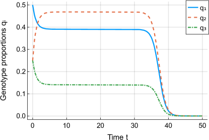
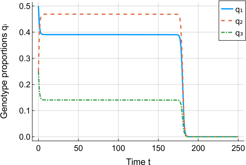
Numerical simulations provide a first impression of the spread of the genotypes over time. At first, we use the fifth-order Runge-Kutta method of Tsitouras [27], which is the recommended default method for non-stiff problems in OrdinaryDiffEq.jl [17]. As shown in Figure 1, the numerical solution appears to converge to a steady state — until it suddenly goes to zero. While the tendency towards the steady state matches our expectation, the decay to zero contradicts the modeling assumption $\sum_{i}q_{i}=1$ and does not change significantly if we use stricter tolerances — the time of “extinction” may only be postponed a bit.

Figure 1: Numerical solution of the system (2.8) with initial condition $q_{0}=(0.5,0.25,0.25)^{T}$ obtained by the fifth-order Runge-Kutta method of Tsitouras [27] implemented in OrdinaryDiffEq.jl [17] in Julia [2] with absolute and relative tolerances $10^{-8}$.

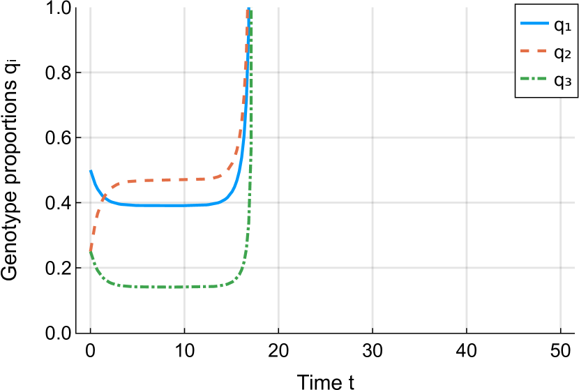
The method of Tsitouras is tested quite well in practice. But maybe something is wrong with it for this specific problem? To double-check the results, we also apply the classical fifth-order method of Dormand and Prince [5] well-known from ode45 in MATLAB [23]. The short-term results shown in Figure 2 are the same as before. However, this time the numerical solutions blow up instead.

(a) Zoom-in.

(b) Zoom-out.

Figure 2: Numerical solution of the system (2.8) with initial condition $q_{0}=(0.5,0.25,0.25)^{T}$ obtained by the fifth-order Runge-Kutta method of Dormand and Prince [5] implemented in OrdinaryDiffEq.jl [17] in Julia [2] with absolute and relative tolerances $10^{-8}$. (a) Focus on the tendency towards steady states, (b) Change of the system behavior to blow up.

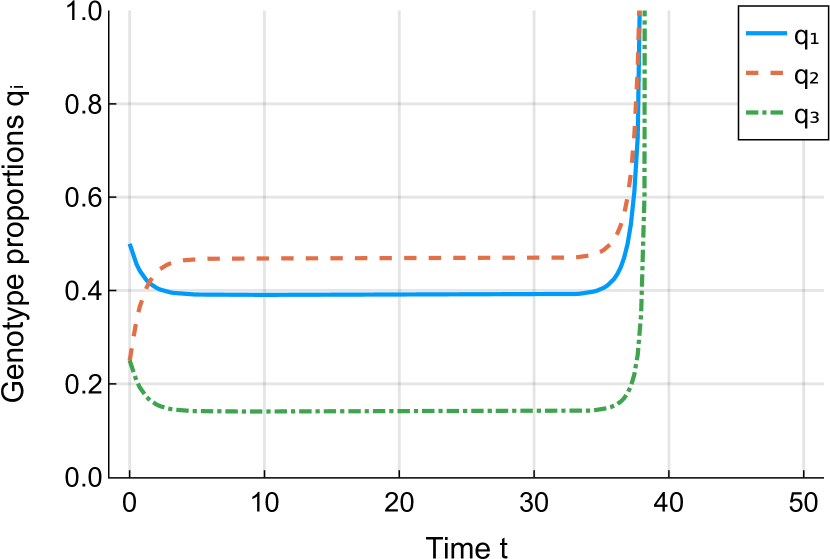
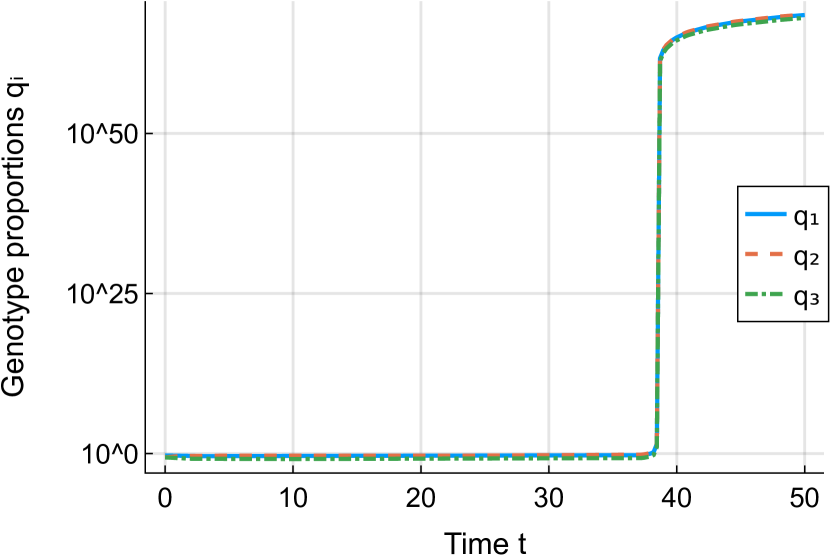
The results for both methods do not change significantly if we use stricter tolerances. We have also tested other methods (explicit and implicit Runge-Kutta methods, Rosenbrock-type methods, multistep methods) implemented in a variety of software packages and programming languages. The results are all similar to the two prototypical examples shown above — both contradicting the behavior we expected from the models. This is certainly something we need to understand.

3 Dynamical system analysis

As numerical simulations show surprising behavior of the solutions, we have a deeper look at the analysis of the dynamical systems. The aim is to understand why the numerical simulations fail and to get ideas on how to overcome these difficulties by changing the system.

3.1 A reduced 2-component model

For some easier visualization, we regard an inheritance model for only two genotypes ($q_{1}$ and $q_{2}$) and one allele, including some mutation. The mutation describes an outcome of genotype $q_{i}$ if the parent generation has the genotype $q_{j}$ with $i\neq j$. Given a parameter $a\in(0,1)$, the dynamics read

$$q_{1}^{\prime} =f_{1}(q)=aq_{1}^{2}+q_{1}q_{2}+(1-a)q_{2}^{2}-q_{1},$$ (3.1)

$$q_{2}^{\prime} =f_{2}(q)=(1-a)q_{1}^{2}+q_{1}q_{2}+aq_{2}^{2}-q_{2}.$$

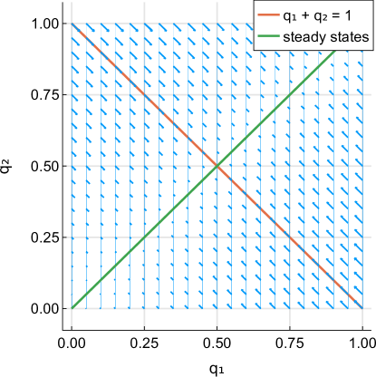
The vector field visualization in Figure 3 illustrates the dynamics of the system.

The system (3.1) has two steady states, $(0,0)^{T}$ and $(1/2,1/2)^{T}$, where only the latter fulfills the conservation condition $q_{\mathrm{sum}}=q_{1}+q_{2}=1$ and therefore lies on the hyperplane given by $q_{2}=1-q_{1}$. This line represents an invariant manifold for $q_{\mathrm{sum}}$ fulfilling the conservation condition. The trivial steady state $q^{\star}=0$ is stable while the non-trivial steady state is unstable. Figure 3 shows this behavior since initial values with $q_{1}+q_{2}<1$ have trajectories leading to the trivial steady state. Initial conditions with $q_{1}+q_{2}>1$ have trajectories with $\lim_{t\to\infty}q_{i}(t)=\infty$.

Figure 3: Visualization of the vector field $f$ of the 2-component system (3.1) with $a=0.7$. The invariant manifold given by $q_{1}+q_{2}=1$ is highlighted. The length of the lines is proportional to $\sqrt{\|f(q)\|}$.

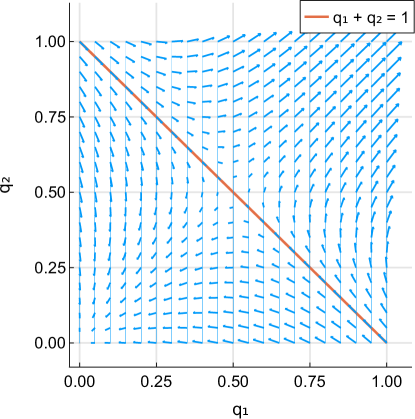
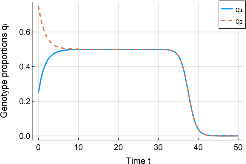
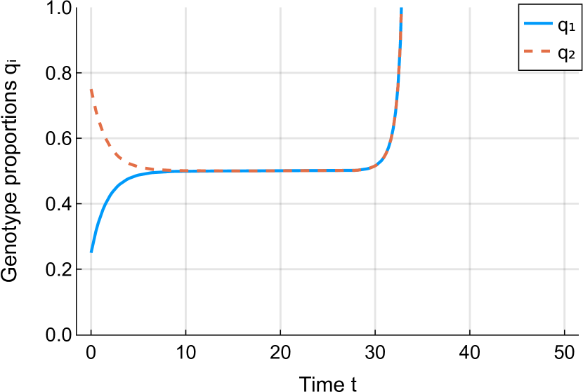
Numerical solutions of (3.1) behave qualitatively similar to their analogs for the 3-component model (2.8): The numerical solutions shown in Figure 4 seem to converge to the (unstable) steady state $(1/2,1/2)^{T}$ at first but eventually go to zero (the stable steady state) or blow up.

(a) Tsitouras.

(b) Verner.

Figure 4: Numerical solution of the system (3.1) with $a=0.7$ and initial condition $q_{0}=(0.25,0.75)^{T}$ obtained by the fifth-order Runge-Kutta method of Tsitouras [27] and the sixth-order method of Verner [28] implemented in OrdinaryDiffEq.jl [17] in Julia [2] with absolute and relative tolerances $10^{-8}$. For these tolerances, the method of Dormand and Prince [5] yields a numerical solution going to zero.

3.2 Analysis of the 3-component model

Now, we investigate the steady states of the system (2.8), so $q^{\star}$ with $f_{i}(q^{\star})=0$ for $i=1,2,3$.

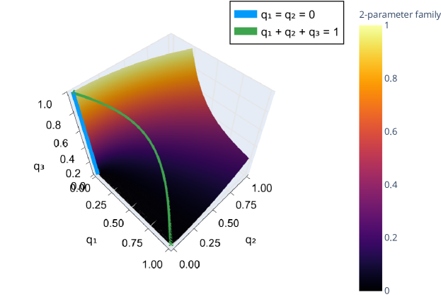
Solving the equation gives a one-parameter family of non-negative steady states

$$q^{\star}=\left(q_{1}^{\star},2\left(\sqrt{q_{1}^{\star}}-q_{1}^{\star}\right),1+q_{1}^{\star}-2\sqrt{q_{1}^{\star}}\right)^{T},\qquad q_{1}^{\star}\in[0,1],$$ (3.2)

fulfilling the conservation condition $\sum_{i=1}^{3}q_{i}^{\star}=1$ and reflecting the binomial distribution of the two alleles. The trivial state $q^{\star}=0\in\mathbb{R}^{3}$ is a steady state as well but does not fulfill the conservation condition.

To investigate the stability properties of the steady states, we compute the eigenvalues of the Jacobian

$$f^{\prime}(q)=\begin{pmatrix}-1+2q_{1}+q_{2}&q_{1}+q_{2}/2&0\\ q_{2}+2q_{3}&-1+q_{1}+q_{2}+q_{3}&2q_{1}+q_{2}\\ 0&q_{2}/2+q_{3}&-1+q_{2}+2q_{3}\end{pmatrix}.$$ (3.3)

Its eigenvalues are $\lambda_{k}=-1+k\sum_{i=1}^{3}q_{i}$, $k\in\{0,1,2\}$, with associated eigenvectors

$$v_{0}=\begin{pmatrix}1\\ -2\\ 1\end{pmatrix},\quad v_{1}=\begin{pmatrix}-(2q_{1}+q_{2})\\ 2(q_{1}-q_{3})\\ q_{2}+2q_{3}\end{pmatrix},\quad v_{2}=\begin{pmatrix}(2q_{1}+q_{2})^{2}\\ 2(2q_{1}+q_{2})(q_{2}+2q_{3})\\ (q_{2}+2q_{3})^{2}\end{pmatrix},$$ (3.4)

for $q\neq 0$; $f^{\prime}(0)=-\operatorname{I}$ has the eigenvalue $-1$ with multiplicity three. In particular, the non-trivial steady states are unstable with eigenvalues $-1$, $0$, and $1$. The trivial steady state $q^{\star}=0$ is asymptotically stable. All of these non-negative steady states are visualized in Figure 5.

Figure 5: Non-negative steady states of the system (2.8). All non-trivial steady states are unstable.

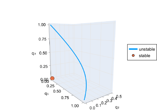
The dynamical system analysis allows us to answer the first question of why we are having unstable numerical simulations: The steady states on the hyperplane with $\sum_{i}q_{i}=1$ are unstable, both for the 2-component system (3.1) and for the 3-component system (2.8). Useful tools for gaining these information are either the visualization of the dynamical system as a vector field or the analysis of the eigenvalues of the Jacobian. The preferred method depends on the dimension of the problem.

Small perturbations occurring from floating point errors in the numerical simulations make the system leave the (unstable) hyperplane with $\sum_{i}q_{i}=1$ and the solutions tend to zero or blow up.

The next question there is, how we can overcome these difficulties.

4 Using invariants for gaining better models

The systems (2.8) and (3.1) are constructed under the assumption that the total amount $\sum_{i}q_{i}=1$ is conserved. From a modeling perspective, this property seems to remain unchanged for the differential equation system and therefore gives an invariant. Numerical simulations show that $\sum_{i}q_{i}$ is not conserved during the simulations. The analysis of the steady states even proves the instability of steady states fulfilling $\sum_{i}q_{i}=1$.

4.1 Qualitative properties of invariants

The question of how to overcome these problems leads us to the analysis of invariants.

Definition 4.1 (First integrals, cf. Section 2.1 of [8]).

Let $U\subset\mathbb{R}^{M}$ be open. Consider the ODE $q^{\prime}=f(q)$ with $f\colon U\to\mathbb{R}^{M}$. A (time-independent) first integral of the ODE is a $C^{1}$-function $J\colon U\to\mathbb{R}$ with $J^{\prime}(q)\cdot f(q)=0$ for all $q\in U$. The first interval is called trivial if $\exists c\,\forall q\in U\colon J(q)=c$.

Clearly, a first integral is an invariant of the ODE, i.e., it does not change along a solution trajectory. Indeed, if $q$ solves the ODE $q^{\prime}(t)=f\bigl{(}q(t)\bigr{)}$,

$$\frac{\operatorname{d\!}}{\operatorname{d\!}t}J\bigl{(}q(t)\bigr{)}=J^{\prime}\bigl{(}q(t)\bigr{)}\cdot q^{\prime}(t)=J^{\prime}\bigl{(}q(t)\bigr{)}\cdot f\bigl{(}q(t)\bigr{)}=0.$$ (4.1)

We first prove that the sum $\sum_{i}q_{i}$ is not a first integral for (2.8). The functional $J(q)=\sum_{i}q_{i}$ has the gradient $(1,1,1)^{T}$. Thus,

$$J^{\prime}(q)\cdot f(q) =\left(\frac{\partial}{\partial q}\sum_{i}q_{i}\right)\cdot f(q)=\sum_{i}f_{i}$$ (4.2)

$$=q_{1}^{2}+q_{2}^{2}+q_{3}^{2}+2q_{1}q_{2}+2q_{1}q_{3}+2q_{2}q_{3}-q_{1}-q_{2}-q_{3}$$

$$=(q_{1}+q_{2}+q_{3})^{2}-(q_{1}+q_{2}+q_{3})\neq 0$$

in general. An analogous result holds for the 2-component model. Thus, the systems (2.8) and (3.1) do not conserve the sum $J(q)=\sum_{i}q_{i}$ for all chosen initial values. But once we choose initial values fulfilling $\sum_{i}q_{i}=1$, the analytical solution does not leave the level set of $J$. Second integrals take this property into account:

Definition 4.2 (Second integrals, cf. Section 2.5 of [8]).

Let $U\subset\mathbb{R}^{M}$ be an open subset. Consider the ODE $q^{\prime}=f(q)$ with $f\colon U\to\mathbb{R}^{M}$. A second integral of the ODE $q^{\prime}(t)=f\bigl{(}q(t)\bigr{)}$ with vector field $f\colon U\to\mathbb{R}^{M}$ is a $C^{1}$-function $J\colon U\to\mathbb{R}$ such that there is a function $\alpha\colon U\to\mathbb{R}$ satisfying $\forall q\in U\colon J^{\prime}(q)\cdot f(q)=\alpha(q)J(q)$.

Clearly, second integrals $J$ are conserved by solutions of the ODE whenever the initial conditions starts on the manifold given by $J(q)=0$.

The systems (2.8) and (3.1) have the total sum $\sum_{i}q_{i}=1$ as a second integral. The difference $u\mathrel{\mathop{\ordinarycolon}}=\sum_{i}q_{i}-1$ between the total sum and unity satisfies

$$u^{\prime}=\sum_{i}q_{i}^{\prime}=\biggl{(}\sum_{i}q_{i}\biggr{)}^{2}-\biggl{(}\sum_{i}q_{i}\biggr{)}=(1+u)^{2}-(1+u)=(1+u)u.$$ (4.3)

All Runge-Kutta methods preserve such linear second integrals [26].

The ODE (4.3) is very similar to the ODE of logistic growth and can be solved analytically,

$$u(t)=\frac{u_{0}}{\mathrm{e}^{-t}(1+u_{0})-u_{0}},\qquad u_{0}=u(0).$$ (4.4)

This ODE (4.3) has two steady states, the unstable steady state $u=0$, corresponding to $\sum_{i}q_{1}=1$, and the asymptotically stable steady state $u=-1$ corresponding to $\sum_{i}q_{i}=0$. For an initial condition $u_{0}<0$, $u(t)\to-1$ for $t\to\infty$. For initial data $u_{0}>0$, $u(t)$ grows without bounds and blows up in finite time. We discovered this behavior for the 2-component model in Fig. 4.

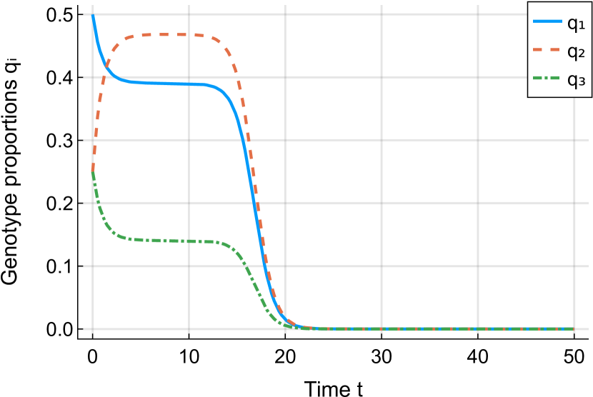
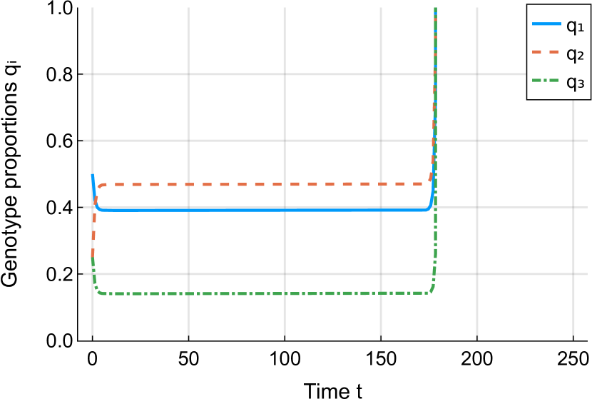
An initial condition of the original model (2.8) needs to satisfy $\sum_{i}q_{i}=1$. Thus, the system (4.3) is in the unstable steady state. When solving (2.8) numerically, it can be expected that even tiny floating point errors can accumulate over time, either resulting in a blow-up in finite time or a convergence to the biologically meaningless state $\sum_{i}q_{i}=0$. To verify this, we also performed computations using different floating point types. The results shown in Figure 6 are qualitatively the same as before, only the time where deviations from the steady state become visible change.

(a) Tsitouras, Float32.

(b) Tsitouras, BigFloat.

(c) Dormand and Prince, Float32.

(d) Dormand and Prince, BigFloat.

Figure 6: Numerical solution of the system (2.8) with initial condition $q_{0}=(0.5,0.25,0.25)^{T}$ obtained by the fifth-order Runge-Kutta methods of Tsitouras [27] and Dormand and Prince [5] implemented in OrdinaryDiffEq.jl [17] in Julia [2] with different floating point types. For 32 bit floating point numbers Float32 we use tolerances $10^{-7}$. For high-precision floating point numbers BigFloat, we use stricter tolerances $10^{-14}$.

To overcome these issues, we reformulate the system so that the total sum becomes a first integral. First, we present a general result showing that this is possible.

Theorem 4.3.

Consider an ODE $q^{\prime}(t)=f\bigl{(}q(t)\bigr{)}$ with affine second integral $J$. Then, there is a modified vector field $\widetilde{f}$ having $J$ as first integral such that

$$\forall y\colon\quad J(y)=0\implies f(y)=\widetilde{f}(y).$$

In particular, the original ODE is equivalent to the modified ODE $\widetilde{q}^{\prime}(t)=\widetilde{f}(\widetilde{q}(t)))$ whenever the initial condition is in the zero set of $J$. The modified vector field $\widetilde{f}$ can be constructed as $\widetilde{f}(y)=f(y)-\alpha(y)J^{\prime}(y)/\|J^{\prime}(y)\|^{2}J(y)$, where we interpret the gradient $J^{\prime}(y)$ as vector field.

Proof.

We have $J^{\prime}(y)\cdot f(y)=\alpha(y)J(y)$. Choose the ansatz $\widetilde{f}(y)=f(y)+J(y)c$ where $c$ is a constant vector that will be suitably chosen. Then,

$$J^{\prime}(y)\cdot\widetilde{f}(y)=J^{\prime}(y)\cdot f(y)+J(y)J^{\prime}(y)\cdot c=\left(\alpha(y)+J^{\prime}(y)\cdot c\right)J(y).$$

Since $J$ is affine, $J^{\prime}(y)$ is constant. If $J^{\prime}(y)=0$, $J(y)=c$ and $J$ is already a (trivial) first integral and $c$ can be chosen arbitrarily. Otherwise, choose e.g. $c=-\alpha(y)J^{\prime}(y)/\|J^{\prime}(y)\|^{2}$ and obtain $J^{\prime}(y)\cdot\widetilde{f}(y)=0$. Thus, $J$ is a first integral of the vector field $\widetilde{f}$. ∎

We will see, that various choices of the coefficient $c$ used in the proof above are possible, leading to different modified models. Further, the modification changes the set of steady states of the ODE leading to different numerical behavior.

4.2 Reformulation of the models

The theory of invariants allows reformulations of the system. The aim is to modify the system in such a way that the stability properties of the steady states improve while retaining the dynamic behavior. We cannot expect to have asymptotically stable steady states but having stable steady states is already an improvement. Then, numerical simulations will be stable and floating point errors do not change the qualitative behavior of the system.

4.2.1 Reformulation of the 2-component model

We start with reformulating the system (3.1) intuitively by using the property $q_{1}+q_{2}=1$. First, we reorder the system as

$$q_{1}^{\prime}=aq_{1}^{2}+q_{1}\underbrace{(q_{2}-1)}_{=-q_{1}}+(1-a)q_{2}^{2},\quad q_{2}^{\prime}=(1-a)q_{1}^{2}+\underbrace{(q_{1}-1)}_{=-q_{2}}q_{2}+aq_{2}^{2}.$$ (4.5)

Replacing $q_{2}-1=-q_{1}$ in the first equation and $q_{1}-1=-q_{2}$ in the second gives the new system

$$q_{1}^{\prime} =(1-a)\bigl{(}-q_{1}^{2}+q_{2}^{2}\bigr{)},$$ (4.6)

$$q_{2}^{\prime} =(1-a)\bigl{(}q_{1}^{2}-q_{2}^{2}\bigr{)}.$$

In this system, the sum of the components is a first integral since $q_{1}^{\prime}+q_{2}^{\prime}=0$ without any further assumptions.

Remark 4.4.

The process of changing a dynamical system such that an (affine) second integral becomes a first integral is not unique.

A second integral for system (3.1) is given by $J=u=\sum_{i}q_{i}-1$ in (4.3). Indeed, choosing the function $\alpha(q)=\sum_{i}q_{i}$ yields the defining equation $J^{\prime}(q)\cdot f(q)=\alpha(q)J(q)$. Based on the second integral $J$ we reformulate the system as $\widetilde{f}(q)=f(q)+J(q)c$.

Our intuitive approach leading to system (4.6) uses the special choice $c=-q$. We prove by a calculation that the modified system has a first integral: The function $\alpha(q)=\sum_{i}q_{i}$ can be written as $\alpha(q)=J^{\prime}(q)\cdot q$ with $J(q)=\sum_{i}q_{i}-1$. The new vector field $\widetilde{f}$ is given as $\widetilde{f}(q)=f(q)-J(q)q$ and the new ODE has a first integral because

$$\frac{\operatorname{d\!}}{\operatorname{d\!}t}J\bigl{(}q(t)\bigr{)}=J^{\prime}(q)\cdot\widetilde{f}(q)=J^{\prime}(q)\cdot f(q)-J^{\prime}(q)\cdot J(q)q=\alpha(q)J(q)-J^{\prime}(q)\cdot J(q)q=0,$$ (4.7)

where we first use the definition of $\widetilde{f}$, then the second integral property of $f$ and thirdly the observation that $\alpha(q)=J^{\prime}(q)\cdot q$.

On the other hand, the modified vector field $\widetilde{f}$ constructed in the proof of Theorem 4.3 with $c=-\alpha(q)J^{\prime}(q)/\|J^{\prime}(q)\|^{2}$ yields the ODE

$$q_{1}^{\prime} =\left(aq_{1}^{2}+q_{1}q_{2}+(1-a)q_{2}^{2}-q_{1}\right)-\frac{1}{2}\left((q_{1}+q_{2})^{2}-(q_{1}+q_{2})\right)$$ (4.8)

$$=(a-1/2)(q_{1}^{2}-q_{2}^{2})-\frac{1}{2}(q_{1}-q_{2}),$$

$$q_{2}^{\prime} =\left((1-a)q_{1}^{2}+q_{1}q_{2}+aq_{2}^{2}-q_{2}\right)-\frac{1}{2}\left((q_{1}+q_{2})^{2}-(q_{1}+q_{2})\right)$$

$$=(1/2-a)(q_{1}^{2}-q_{2}^{2})+\frac{1}{2}(q_{1}-q_{2}),$$

for the 2-component model (3.1). This is clearly different from (4.6) in general (but of course equivalent on the invariant manifold).

We continue our investigations with the new system (4.6). This system has the non-negative steady states $(q_{1}^{\star},q_{1}^{\star})^{T}$ with $q_{1}^{\star}\geq 0$. For $q_{1}^{\star}\neq 1/2$, the steady states do not fulfill the condition $\sum_{i=1}^{2}q_{i}=1$. The vector field is shown in Figure 7. For any initial conditions, the dynamics lead to a steady state $(q_{1}^{\star},q_{1}^{\star})^{T}$ with $q_{1}^{\star}=1/2\,(q_{1}(0)+q_{2}(0))$.

Figure 7: Visualization of the right-hand side vector field $f$ of the modified 2-component system (4.6) with $a=0.7$. The invariant manifold given by $q_{1}+q_{2}=1$ is highlighted. The length of the lines is proportional to $\sqrt{\|f(q)\|}$.

The stability of the steady states can be assured by calculating the eigenvalues of the Jacobian of the system. The Jacobian

$$f^{\prime}(q)=2(1-a)\begin{pmatrix}-q_{1}&q_{2}\\ q_{1}&-q_{2}\end{pmatrix}$$ (4.9)

has the eigenvalues $\lambda_{0}=0$ and $\lambda_{1}=-2(1-a)(q_{1}+q_{2})<0$ with eigenvectors

$$v_{0}=\begin{pmatrix}q_{2}\\ q_{1}\end{pmatrix},\quad v_{1}=\begin{pmatrix}-1\\ 1\end{pmatrix},$$ (4.10)

for $q\neq 0$; $f^{\prime}(0)=0$ has the double eigenvalue $0$. Consequently, the non-trivial steady states are stable.

Starting with any initial values $q_{1},q_{2}>0$, the solutions tend towards the steady states. If the initial conditions fulfill the condition $\sum_{i}q_{i}=1$ of the hyperplane, the solutions remain on the hyperplane. Deviations on the manifold, for example caused by floating point errors, will not change the overall system behavior and result in deviations of the steady state from the hyperplane. For this model, a transformation of variables to $p_{1}=q_{1}+q_{2}$ and $p_{2}=q_{2}-q_{1}$ separates the tendency towards the hyperplane from the stationary behavior on the manifold but would change the interpretability of the variables.

Remark 4.5.

The stability of steady states of the modified 2-component system (4.6) can be understood easily by looking at Figure 7.

This behavior is also generic in the sense that it can be obtained from the center manifold theorem — at least locally, see [10, Theorem I.4] or [14, Theorem 2.7]. Summarized briefly, the center manifold theorem states that a dynamical system near a steady state where all eigenvalues of the Jacobian have a non-negative real part behaves as follows: i) There is a neighborhood $V$ of the steady state and a manifold $M$ of the same dimension as the generalized eigenspace associated with eigenvalues on the imaginary axis that is invariant under the flow as long as the evolving state stays in $V$. ii) If the state stays in $V$ for all times, it converges (exponentially) to the manifold $M$. In our case, the eigenvalue on the imaginary axis is zero and the corresponding manifold is the set of steady states.

4.2.2 Reformulation of the 3-component model

Inserting the conservation condition $\sum_{i=1}^{3}q_{i}=1$ into the first equation of (2.8) yields

$$q_{1}^{\prime}=q_{1}^{2}+q_{1}q_{2}+\frac{1}{4}q_{2}^{2}-q_{1}\underbrace{(q_{1}+q_{2}+q_{3})}_{=1}=\frac{1}{4}q_{2}^{2}-q_{1}q_{3}.$$ (4.11)

Continuing this process for the other equations as well results in the modified system

$$q_{1}^{\prime} =\frac{1}{4}q_{2}^{2}-q_{1}q_{3},$$ (4.12)

$$q_{2}^{\prime} =-\frac{1}{2}q_{2}^{2}+2q_{1}q_{3},$$

$$q_{3}^{\prime} =\frac{1}{4}q_{2}^{2}-q_{1}q_{3}.$$

Again, as in the case of the 2-component model, this reformulation can be interpreted as turning the second integral $J(q)=u(q)=\sum_{i}q_{i}-1$ with $\alpha(q)=\sum_{i}q_{i}$ into a first integral for the new vector field $\widetilde{f}=f-J(q)q$. The calculations in Remark 4.4 are valid as well for the 3-component system.

The modified system (4.12) has the non-negative steady state $q^{\star}=(q_{1}^{\star},q_{2}^{\star},q_{3}^{\star})^{T}$ with

$$q_{3}^{\star}=\begin{cases}\text{arbitrary}\geq 0,&\text{if }q_{1}^{\star}=q_{2}^{\star}=0,\\ \frac{q_{2}^{\star 2}}{4q_{1}^{\star}},&\text{if }q_{1}^{\star}\neq 0,\end{cases}$$ (4.13)

for $q_{1}^{\star},q_{2}^{\star}\geq 0$ and $q_{2}^{\star}=0$ if $q_{1}^{\star}=0$. Note in particular that the steady states of (4.12) satisfying $\sum_{i}q_{i}=1$ are exactly the non-trivial steady states of the original system (2.8). The Jacobian is

$$f^{\prime}(q)=\begin{pmatrix}-q_{3}&q_{2}/2&-q_{1}\\ 2q_{3}&-q_{2}&2q_{1}\\ -q_{3}&q_{2}/2&-q_{1}\\ \end{pmatrix}.$$ (4.14)

For $q\neq 0$, $f^{\prime}(q)$ has a double eigenvalue $\lambda_{0}=\lambda_{1}=0$ with eigenspace spanned by

$$v_{0}=\begin{pmatrix}q_{1}\\ 0\\ -q_{3}\end{pmatrix},\quad v_{1}=\begin{pmatrix}q_{2}/2\\ q_{1}+q_{3}\\ q_{2}/2\end{pmatrix},$$ (4.15)

as well as the eigenpair

$$\lambda_{2}=-\sum_{i=1}^{3}q_{i},\quad v_{2}=\begin{pmatrix}1\\ -2\\ 1\end{pmatrix}.$$ (4.16)

Moreover, $f^{\prime}(0)=0$. Thus, all non-negative steady states are associated with eigenvalues of $f^{\prime}(q)$ with non-positive real parts. The non-negative steady states are visualized in Figure 8.

Figure 8: Non-negative steady states of the system (4.12). The system Jacobian has only eigenvalues with non-positive real parts at all steady states.

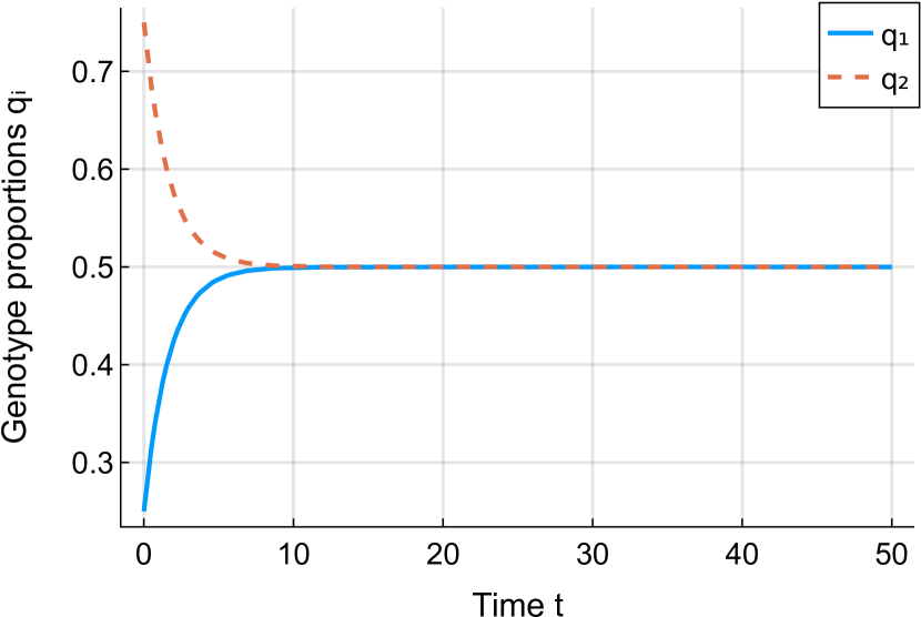
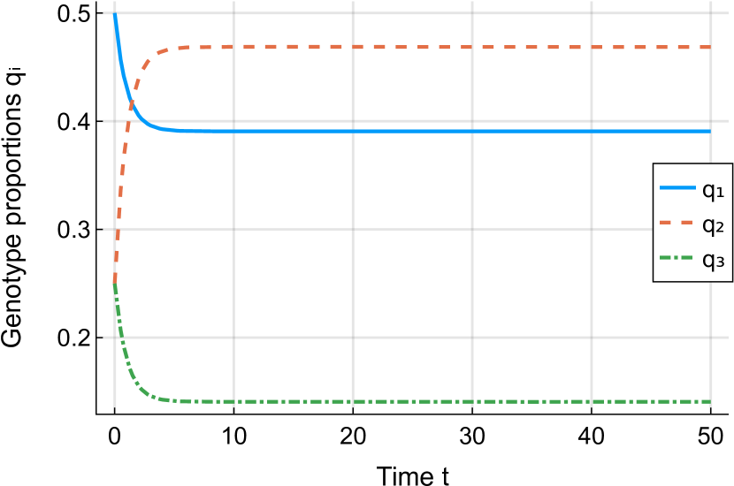
As expected based on this stability analysis, numerical solutions behave properly when applied to the modified systems (4.6) and (4.12). This is demonstrated in Figure 9.

(a) 2-component model.

(b) 3-component model.

Figure 9: Numerical solution of the modified systems (4.6) (with $a=0.7$ and initial condition $q_{0}=(0.25,0.75)^{T}$) and (4.12) (with initial condition $q_{0}=(0.75,0.25,0.25)^{T}$) obtained by the fifth-order Runge-Kutta method of Tsitouras [27] implemented in OrdinaryDiffEq.jl [17] in Julia [2] with absolute and relative tolerances $10^{-8}$.

The modified systems (4.6) and (4.12) have stable steady states fulfilling $\sum_{i}q_{i}^{\star}=1$. The modification of the reaction functions changes the system’s properties from having a second integral to having a first integral.

5 Evaluation of the models

After improving the analytical properties and ensuring the conservation of $\sum_{i}q_{i}$ during the numerical simulations, we like to draw attention to the modeling process.

The models (2.8) and (3.1) were gained quite directly from the biological application. The system quantities $q_{k}$ give the proportion of genotype $k$ in the total population. The condition $\sum_{i}q_{i}=1$ arises therefore naturally from the biological application and the mathematical translation into equations. The biologically motivated models surprised us during the numerical simulations with their unstable behavior arising from leaving the hyperplane with $\sum_{i}q_{i}=1$. Floating point errors already lead to unstable behavior, resulting in solutions tending towards zero or blowing up.

We used the conservation property to reformulate the ordinary differential equation systems. The new systems (4.6) and (4.12) have the same dynamics on the hyperplane as the original models (2.8) and (3.1).

Changing the functions of a model might result in differential equations without any (obvious and direct) connection to the modeling object. Next, we try to interpret the inheritance of genes in the new model (4.12).

Figure 10: Modeled combinations of genes in the original system (2.8) and the modified system (4.12).

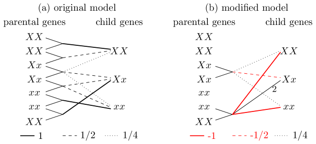
While the system (2.8) translates all combinations of parental genes into equations, the modified system (4.12) regards fewer combinations. The modified system includes only the combination of the mixed genotype $Xx$ and the combination of the two pure genotypes. The combination of two pure genotypes of the same type is not modeled. This can be interpreted as neglecting combinations that do not change the proportions of genotypes in the population. This affects as well the combination $q_{2}$ of two genotypes, since the factor $-1/2$ is the difference between the actual factor $1/2$ in system (2.8) and the factor 1 symbolizing the preservation of genotype $q_{2}$.

The change from system (2.8) to the modified system (4.12) is a change in the point of view: While the first model describes the recombination of genotypes from the point of view of the parental generation, the new model focuses on the change of proportions. In our case, only those combinations are included in the model that change the proportions of the genotypes in the population. Leveling effects, like the inheritance of genotype $q_{1}$ with probability $1/2$ if $q_{1}$ and $q_{2}$ are combined and therefore $1/2$ of the parental genes are identical to the child genes, are not modeled.

A similar interpretation is possible for the 2-component model. As the modified system (4.6) only regards the change of the proportions, the pure conservation of one proportion is not regarded.

Interpretations like this are not automatically possible if a model with a second integral is turned into a model with a first integral. In any case, the new formulation might reveal new perspectives on the application and the most relevant mechanisms in the mathematical description.

6 Conclusion — or what can we learn?

The example we discussed in this article shows how surprising numerical simulation results may lead to insightful analysis and reformulation of mathematical models. The reformulation gives insight in properties of the modeled application on two levels. First, the reformulation process itself sheds light on conservation properties of the model. Second, the new formulation may change the view on the model leading to new interpretations of the mechanisms. Gaining insight into underlying principles is complicated for large models. The proposed reformulation workflow may support the finding of hidden principles while improving the analytical and numerical properties.

Please note that we neither blame the numerics nor the modeling; it is their combination that lead to the catastrophic behavior we discussed. If it was affordable to use exact representations of all numbers occurring in the numerical time integration process, we could just use the original model. However, this is only possible for small problems and short time scales, e.g., by using rational numbers with high-precision integer types such as Rational{BigInt} in Julia. However, it appears to be preferable for us to adapt the modeling process, thereby avoiding the unrealistic instabilities inherent in the original model. This is required for most practical purposes, e.g., if uncertainties are present or larger-scale simulations are used.

To recap, a surprising behavior of numerical methods applied to an innocently looking model from mathematical biology guided us on a tour through several undergraduate and graduate courses including mathematical modeling, dynamical systems, and numerical analysis. In particular, we had a chance to see the importance of invariants and their manifestation in first and second integrals as well as stability properties of steady states.

We would like to see this article as a bridge gathering results and techniques from several basic courses together while motivating advanced courses in applied mathematics. This includes for example deeper concepts of stability analysis, the study of asymptotic behavior of dynamical systems [15, 22], and advanced results such as the center manifold theorem [10, 14] or Fenichel’s theory on invariant manifolds [7] on the theoretical side. The latter emphasizes using transformation to local coordinates on the manifold. While this approach has many analytical benefits, local coordinates are oftentimes difficult to interpret in the context of applications.

From the point of view of a numerical analyst, it stresses the importance of structure-preserving numerical methods, introduced in textbooks such as [21, 9] in the context of numerical methods for ODEs; the corresponding partial differential equation topics appear to be more specialized and available mostly in form of journal articles such as [25, 6, 18, 19]. The basic reason for us to modify the mathematical models was to stabilize the dynamics when the total sum is not equal to unity. This is related to invariant-preserving numerical methods such as the orthogonal projection approach described in [9, Section IV.4]. However, most numerical analysts would probably not consider using such tools here since we only need to preserve a linear functional — which the standard time integration methods we employ do automatically [26] — at least in exact arithmetic. Thus, the behavior is somewhat surprising but of course well understood after performing a stability analysis. In some sense, we have to deal with non-ideal versions in practice while the common analysis assumes ideal numerical methods. This happens also in many other cases in practice, e.g., if iterative numerical methods are used to solve equations arising in implicit time integration schemes [3, 12, 13].

We introduced the problem of invariants and manifolds in the context of mathematical biology. Of course, problems of this type occur in many applications, for example in control problems [29] or mechanical systems [9]. Finally, we encourage researchers in the field of mathematical modeling and applied sciences to discover the strength of mathematical theory, especially for dynamical systems and for structure-preserving numerical schemes, for gaining insight into the dynamics of interest.

To make this study reproducible and useful for classroom teaching, we provide all source code and instructions available online in our repository [20] — in the form of an interactive notebook using the modern programming language Julia.

References

- [1] Benjamin Allen and Alex McAvoy “A mathematical formalism for natural selection with arbitrary spatial and genetic structure” In Journal of Mathematical Biology 78.4, 2019, pp. 1147–1210 DOI: 10.1007/s00285-018-1305-z
- [2] Jeff Bezanson, Alan Edelman, Stefan Karpinski and Viral B Shah “Julia: A Fresh Approach to Numerical Computing” In SIAM Review 59.1 SIAM, 2017, pp. 65–98 DOI: 10.1137/141000671
- [3] Philipp Birken and Viktor Linders “Conservation Properties of Iterative Methods for Implicit Discretizations of Conservation Laws” In Journal of Scientific Computing 92.2 Springer, 2022, pp. 1–32
- [4] N. F. Britton “Essential mathematical biology”, Springer Undergraduate Mathematics Series London: Springer, 2003 DOI: 10.1007/978-1-4471-0049-2
- [5] John R Dormand and Peter J Prince “A family of embedded Runge-Kutta formulae” In Journal of Computational and Applied Mathematics 6.1 Elsevier, 1980, pp. 19–26 DOI: 10.1016/0771-050X(80)90013-3
- [6] Herbert Egger “Structure preserving approximation of dissipative evolution problems” In Numerische Mathematik 143.1 Springer, 2019, pp. 85–106 DOI: 10.1007/s00211-019-01050-w
- [7] Neil Fenichel and J. K. Moser “Persistence and Smoothness of Invariant Manifolds for Flows” In Indiana University Mathematics Journal 21.3 Indiana University Mathematics Department, 1971, pp. 193–226 URL: http://www.jstor.org/stable/24890380
- [8] Alain Goriely “Integrability and nonintegrability of dynamical systems” 19, Advanced series in nonlinear dynamics World Scientific, 2001
- [9] Ernst Hairer, Christian Lubich and Gerhard Wanner “Geometric Numerical Integration: Structure-Preserving Algorithms for Ordinary Differential Equations” 31, Springer Series in Computational Mathematics Berlin Heidelberg: Springer-Verlag, 2006 DOI: 10.1007/3-540-30666-8
- [10] Gérard Iooss and Moritz Adelmeyer “Topics in Bifurcation Theory and Applications” 3, Advanced series in nonlinear dynamics Singapore: World Scientific, 1998
- [11] Dirk Langemann, Otto Richter and Antje Vollrath “Multi-gene-loci inheritance in resistance modeling” In Mathematical Biosciences 242.2013, 2012, pp. 17–24 DOI: 10.1016/j.mbs.2012.11.010
- [12] Viktor Linders and Philipp Birken “Locally conservative and flux consistent iterative methods”, 2022 arXiv:2206.10943 [math.NA]
- [13] Viktor Linders, Hendrik Ranocha and Philipp Birken “Resolving Entropy Growth from Iterative Methods”, 2023 DOI: 10.48550/arXiv.2302.13579
- [14] Jerrold E Marsden and Marjorie McCracken “The Hopf Bifurcation and Its Applications” 19, Applied Mathematical Sciences New York: Springer, 1976
- [15] Lawrence Perko “Differential equations and dynamical systems”, Texts in applied mathematics 7 New York: Springer, 2001
- [16] Fons Plas, Michiel Dral and Paul Berg “fonsp/Pluto.jl: v0.19.20” Zenodo, 2023 DOI: 10.5281/zenodo.5889169
- [17] Christopher Rackauckas and Qing Nie “DifferentialEquations.jl – A Performant and Feature-Rich Ecosystem for Solving Differential Equations in Julia” In Journal of Open Research Software 5.1 Ubiquity Press, 2017, pp. 15 DOI: 10.5334/jors.151
- [18] Hendrik Ranocha, Dimitrios Mitsotakis and David I Ketcheson “A Broad Class of Conservative Numerical Methods for Dispersive Wave Equations” In Communications in Computational Physics 29.4 Global Science Press, 2021, pp. 979–1029 DOI: 10.4208/cicp.OA-2020-0119
- [19] Hendrik Ranocha et al. “Relaxation Runge-Kutta Methods: Fully-Discrete Explicit Entropy-Stable Schemes for the Compressible Euler and Navier-Stokes Equations” In SIAM Journal on Scientific Computing 42.2 Society for IndustrialApplied Mathematics, 2020, pp. A612–A638 DOI: 10.1137/19M1263480
- [20] Cordula Reisch and Hendrik Ranocha “Reproducibility repository for Modeling still matters: a surprising instance of catastrophic floating point errors in mathematical biology and numerical methods for ODEs”, https://github.com/ranocha/2023_modeling_matters, 2023 DOI: 10.5281/zenodo.7801250
- [21] Jesus Maria Sanz-Serna and Manuel P Calvo “Numerical Hamiltonian Problems” 7, Applied Mathematics and Mathematical Computation London: Chapman & Hall, 1994
- [22] Rüdiger Seydel “Practical Bifurcation and Stability Analysis” 5, Interdisciplinary Applied Mathematics New York, NY: Springer New York, 2010 DOI: 10.1007/978-1-4419-1740-9
- [23] Lawrence F Shampine and Mark W Reichelt “The MATLAB ODE suite” In SIAM Journal on Scientific Computing 18.1 SIAM, 1997, pp. 1–22 DOI: 10.1137/S1064827594276424
- [24] Joseph D Skufca “Analysis Still Matters: A Surprising Instance of Failure of Runge-Kutta-Felberg ODE Solvers” In SIAM Review 46.4 SIAM, 2004, pp. 729–737 DOI: 10.1137/S003614450342911X
- [25] Eitan Tadmor “Entropy stability theory for difference approximations of nonlinear conservation laws and related time-dependent problems” In Acta Numerica 12 Cambridge University Press, 2003, pp. 451–512 DOI: 10.1017/S0962492902000156
- [26] Benjamin K Tapley “On the preservation of second integrals by Runge-Kutta methods”, 2021 arXiv:2105.10929 [math.NA]
- [27] Ch Tsitouras “Runge-Kutta pairs of order 5 (4) satisfying only the first column simplifying assumption” In Computers & Mathematics with Applications 62.2 Elsevier, 2011, pp. 770–775 DOI: 10.1016/j.camwa.2011.06.002
- [28] James H Verner “Numerically optimal Runge-Kutta pairs with interpolants” In Numerical Algorithms 53.2-3 Springer, 2010, pp. 383–396 DOI: 10.1007/s11075-009-9290-3
- [29] R. A. Wehage and E. J. Haug “Generalized Coordinate Partitioning for Dimension Reduction in Analysis of Constrained Dynamic Systems” In Journal of Mechanical Design 104.1, 1982, pp. 247–255 DOI: 10.1115/1.3256318