Canonical Momenta in Digitized SU$(2)$ Lattice Gauge Theory:
Definition and Free Theory

Abstract

Hamiltonian simulations of quantum systems require a finite-dimensional representation of the operators acting on the Hilbert space $\mathcal{H}$. Here we give a prescription for gauge links and canonical momenta of an SU$(2)$ gauge theory, such that the matrix representation of the former is diagonal in $\mathcal{H}$. This is achieved by discretising the sphere $S_{3}$ isomorphic to SU$(2)$ and the corresponding directional derivatives. We show that the fundamental commutation relations are fulfilled up to discretisation artefacts. Moreover, we directly construct the Casimir operator corresponding to the Laplace-Beltrami operator on $S_{3}$ and show that the spectrum of the free theory is reproduced again up to discretisation effects. Qualitatively, these results do not depend on the specific discretisation of SU$(2)$, but the actual convergence rates do.

I Introduction

While the Hamiltonian of lattice gauge theories is known since 1975 Kogut and Susskind (1975), it only recently received a fresh interest. This is due to the development of tensor network state (TNS) and quantum computing (QC) methods over the last few years. These methods promise to provide the possibility to investigate lattice gauge theories (and other quantum systems) in regions of parameter space inaccessible to Monte Carlo methods, most prominently in situations when a sign problem is hindering the application of stochastic methods. In addition, with the Hamiltonian formulation of lattice field theories also real time simulations become possible, opening up new insights in the dynamical properties of physical systems.

Tensor network based methods have been introduced for lattice field theory methods in many works, see, e.g. Refs. Silvi et al. (2014); Dalmonte and Montangero (2016); Bañuls and Cichy (2020); Bañuls et al. (2020, 2019). The success of TNS lies on the fact that only a small subspace of the complete Hilbert space describes the physically often only relevant low energy physics. Therefore, various phenomena such as string breaking and real-time dynamics Buyens et al. (2014); Kühn et al. (2015); Pichler et al. (2016); Buyens et al. (2017); Banuls et al. (2019); Rigobello et al. (2021) or the phase structure of gauge theories at finite fermionic densities Bañuls et al. (2017); Silvi et al. (2017); Felser et al. (2020); Silvi et al. (2019) have been investigated using TNS on moderately large lattice volumes.

More recently, quantum computer simulations have been performed for lattice gauge theories. In this approach, the number of required qubits grows only linearly with the number of lattice sites. There are also proposals to implement real-time dynamics for scalar quantum field theories and quantum electrodynamics Byrnes and Yamamoto (2006); Jordan et al. (2012); Mathis et al. (2020). Since quantum computations use the Hamiltonian formulation, they can completely avoid the sign problem. Quantum computers therefore allow to realise Feynman’s vision to simulate nature on a quantum mechanical, physical system Feynman (1982).

The literature of quantum computations for lattice gauge theories has increased tremendously in the last years, see Refs. Bañuls and Cichy (2020); Bañuls et al. (2020); Klco et al. (2020a); Atas et al. (2021a); Ciavarella et al. (2021a); Clemente et al. (2022). There are various approaches for implementing lattice gauge theories using optical lattices Banerjee et al. (2012); Tagliacozzo et al. (2013a, b), atomic and ultra-cold quantum matter Büchler et al. (2005); Zohar and Reznik (2011); Zohar et al. (2012); Hauke et al. (2013); Zohar et al. (2013a, b); Banerjee et al. (2013); Zohar et al. (2016); Laflamme et al. (2016); González-Cuadra et al. (2017); Rico et al. (2018); Zache et al. (2018), and further proof-of-principle implementations on a real superconducting architecture Klco et al. (2018a, 2020a); Atas et al. (2021a); Ciavarella et al. (2021a); Mazzola et al. (2021) and real-time and variational simulations on a trapped ion system Martinez et al. (2016); Kokail et al. (2019). For recent overviews see Refs. Dalmonte and Montangero (2016); Bañuls and Cichy (2020); Bañuls et al. (2020); Funcke et al. (2023).

A very important aspect of quantum computations is the quest for the most efficient discretisation scheme of the corresponding gauge group needed to apply both, TNS and QC methods, see e.g. Ref. Davoudi et al. (2021). Work in this direction, both for Abelian gauge theories with and without fermions has been performed by a number of groups already, see for instance Refs. Klco et al. (2018b); Lewis and Woloshyn (2019); Paulson et al. (2021); Haase et al. (2021); Nguyen et al. (2022); Clemente et al. (2022). Also for non-Abelian SU$(2)$ and SU$(3)$ lattice gauge theories there are a number of works available Klco et al. (2020b); Atas et al. (2021b); A Rahman et al. (2021); Ciavarella et al. (2021b); A Rahman et al. (2022a); Atas et al. (2022); Catumba et al. (2022); A Rahman et al. (2022b); Gustafson et al. (2022); Farrell et al. (2023a, b). For more algorithmic developments we refer to Refs. Alam et al. (2022); Carena et al. (2022); Gustafson and Lamm (2023). Another possible formulation is provided by the so-called quantum link model Chandrasekharan and Wiese (1997); Brower et al. (1999); Wiese (2021).

In particular for non-Abelian SU$(N_{c})$ lattice gauge theories it is important to understand how to most efficiently digitise the gauge field operators $\hat{U}$ and the corresponding canonical momentum operators $\hat{L}$ and $\hat{R}$ constituting the Hamiltonian

$$\hat{H}=\ \frac{g_{0}^{2}}{4}\sum_{\mathbf{x},c,k}\left(\hat{L}_{c,k}^{2}(\mathbf{x})+\hat{R}_{c,k}^{2}(\mathbf{x})\right)-\frac{1}{2g_{0}^{2}}\sum_{\mathbf{x},k<l}\mathrm{Tr}\,\mathrm{Re}\,\hat{P}_{kl}(\mathbf{x})\,.$$ (1)

In the above sums, $\mathbf{x}$ represent the coordinates of a $d$-dimensional lattice and $k,l$ label the corresponding directions with $\hat{l},\hat{k}$ unit vectors in these directions. $c=1,\ldots,N_{c}^{2}-1$ indexes the generators of the algebra, $g_{0}$ is the (bare) gauge coupling constant and the plaquette operator is defined as

$$\hat{P}_{kl}(\mathbf{x})\ =\ \hat{U}_{k}(\mathbf{x})\,\hat{U}_{l}(\mathbf{x}+\hat{k})\,\hat{U}^{\dagger}_{k}(\mathbf{x}+\hat{l})\,\hat{U}^{\dagger}_{l}(\mathbf{x})\,.$$ (2)

The $\hat{U}$ are the gauge field operators as explained further below and the trace is taken in colour space.

In the literature the first and second sum in eq. 1 are called respectively (chromo-)electric and (chromo-)magnetic part. Most of the investigations of non-Abelian lattice gauge theories in the Hamiltonian formalism chose a basis of the Hilbert space $\mathcal{H}$ such that the electric part is diagonal. This leads for instance to the so-called character expansion or loop-string formulations, the status of which is elaborately discussed in Ref. Davoudi et al. (2022).

In this paper we are going to explore a different pathway: following the ideas discussed for U$(1)$ in Refs. Haase et al. (2021); Clemente et al. (2022) we will develop a formulation with a basis of $\mathcal{H}$ in which the non-Abelian gauge field operators are diagonal. For this purpose we use the digitisations we recently proposed in Ref. Hartung et al. (2022); Jakobs et al. (2023), which provide a natural discretised parametrization of SU$(2)$ and which can be extended to larger $N_{c}$-values. For more works related to digitised SU$(N_{c})$ gauge fields see Refs. Ji et al. (2020); Alexandru et al. (2019, 2022); Ji et al. (2022).

The remaining task is to find the corresponding digitised versions of the operators $\hat{L},\hat{R}$ or directly the Casimir operator $\hat{L}^{2}+\hat{R}^{2}$, which we are going to discuss in the following. We will show that it is possible to find discrete versions of $\hat{L},\hat{R}$ fulfilling the fundamental commutation relations up to discretisation effects. Moreover, we show that in order to reproduce the spectrum of the free Hamiltonian, the aforementioned Casimir operator needs to be discretised directly. If this is done, spectrum and eigenstates of the free Hamiltonian are reproduced up to discretisation effects, the size of which depends on the specific choice of the partitioning of SU$(2)$.

II Commutators and State Space

To be concrete, we define the set of coordinates of the $d$-dimensional spatial lattice as

$$\Lambda\ =\ \{\mathbf{x}\in\mathbb{R}^{d}:x_{k}=0,a,2a,\ldots,(L_{k}-1)a\}\,,$$

with $k$ labelling the directions as above. $a$ is the lattice spacing which we set to $a=1$ in the following and $L_{k}\in\mathbb{N}$ the lattice extent in direction $k$. The quantization conditions are imposed at each point of the space time lattice. This gives freedom for any choice of the boundary conditions, which are inessential for the rest of our discussion.

States on the full lattice are constructed by tensor products of basis states for each lattice site and direction. This is why it is sufficient to discuss the discretisation for one lattice site and direction and, thus, we will drop the spatial coordinates $\mathbf{x}$ and the directions $k$.

Classically, for each lattice site and direction the gauge link $U$ is an SU$(N_{c})$ matrix in the fundamental representation, with $N_{c}^{2}$ elements $u_{ij}$. On the quantum level, the elements of the gauge fields $\hat{u}_{ij}\in\mathbb{L}$ become operators, with $\mathbb{L}$ the linear operators $\mathcal{H}\to\mathcal{H}$. Now, $\hat{U}$ is a $N_{c}\times N_{c}$ operator valued matrix, which is constrained as follows: given a gauge field state $|U\rangle\in\mathcal{H}$ of the system with $\hat{U}|U\rangle=U|U\rangle$ we require that $U\in\mathrm{SU}(N_{c})$ in the fundamental representation. $\hat{L}_{c},\hat{R}_{c}\in\mathbb{L}$ on the other hand represent the corresponding canonical momenta (in the adjoint representation), which are generating the left and right gauge transformations.

Given the $\hat{U}$, the momenta are defined via the fundamental commutation relations

$$[\hat{L}_{c},\hat{U}_{mn}]\ =\ (t_{c})_{mj}\,\hat{U}_{jn}\,,\qquad[\hat{R}_{c},\hat{U}_{mn}]\ =\ \hat{U}_{mj}(t_{c})_{jn}\,.$$ (3)

Here, $t_{c}$ are the generators of the corresponding Lie algebra. Moreover, the $\hat{L}_{c}$ resemble the group structure

$$[\hat{L}_{a},\hat{L}_{b}]=f_{abc}\hat{L}_{c}\,,$$ (4)

with the the structure constants $f_{abc}$ of the algebra, and likewise the $\hat{R}_{c}$.

Specifically, for SU$(2)$, the generators are given by the Pauli matrices $t_{c}$ with indices $c=1,2,3$. We parametrise the basis for the gauge field states as follows: $U\in$SU$(2)$ can be parametrised with three real valued parameters $y_{0},y_{1},y_{2}$ as follows

$$U=\begin{pmatrix}y_{0}+\mathrm{i}y_{1}&y_{2}+\mathrm{i}y_{3}\\ -y_{2}+\mathrm{i}y_{3}&y_{0}-\mathrm{i}y_{1}\\ \end{pmatrix}\,,\quad y_{3}^{2}=1-\sum_{i=0}^{2}y_{i}^{2}\,.$$ (5)

Since SU$(2)$ is isomorphic to the sphere $S_{3}$, we can also write $y=(y_{0},y_{1},y_{2},y_{3})^{t}\in S_{3}$. Accordingly, we define operators $\hat{y}_{j}:\mathcal{H}\to\mathcal{H}$ by the following action

$$\hat{y}_{j}|U(y)\rangle\ =\ y_{j}|U(y)\rangle\,,\quad j=0,1,2,3\,,$$

and

$$\begin{split}\hat{u}_{00}=\hat{y}_{0}+\mathrm{i}\hat{y}_{1}\,,\quad\hat{u}_{01}=\hat{y}_{2}+\mathrm{i}\hat{y}_{3}\,,\\ \hat{u}_{10}=-\hat{y}_{2}+\mathrm{i}\hat{y}_{3}\,,\quad\hat{u}_{11}=\hat{y}_{0}-\mathrm{i}\hat{y}_{1}\,.\\ \end{split}$$

This defines the action of $\hat{U}:\mathcal{H}\to\mathcal{H}$ on a given state via

$$\hat{U}=\begin{pmatrix}\hat{u}_{00}&\hat{u}_{01}\\ \hat{u}_{10}&\hat{u}_{11}\\ \end{pmatrix}\,.$$

Therefore, the $y_{0,1,2}$ can be regarded as quantum numbers labelling the states $|y_{0},y_{1},y_{2}\rangle\equiv|U(y)\rangle$ which are simultaneous eigenstates of operators $\hat{y}_{0,1,2}$.

Alternatively, one could also work with three angles $\vec{\alpha}$ which can be used to parametrise $U=\exp(\mathrm{i}\,\vec{\alpha}\cdot\vec{t})$. Given $\vec{\alpha}$, the $y_{i}$ can be readily computed. For quantisation, each angle $\alpha_{i}$ is then promoted to a linear operator $\mathcal{H}\to\mathcal{H}$.

Formally, the canonical momenta are defined as Lie derivatives:

$$\begin{split}\hat{L}_{c}\,f(U)\ &=-\mathrm{i}\frac{\mathrm{d}}{\mathrm{d}\beta}\,f\left(e^{\mathrm{i}\,\beta t_{c}}\,U\right)|_{\beta=0}\,,\\ \qquad\hat{R}_{c}\,f(U)\ &=-\mathrm{i}\frac{\mathrm{d}}{\mathrm{d}\beta}\,f\left(U\,e^{\mathrm{i}\,\beta t_{c}}\right)|_{\beta=0}\end{split}$$ (6)

for a function $f(U)$, $f:\mathrm{SU}(2)\rightarrow\mathbb{R}$.

The states parametrised by $y_{0},y_{1}$ and $y_{2}$ can be discretised using one of the partitionings we proposed in Ref. Hartung et al. (2022), or any other partitioning of SU$(2)$. In fact, the precise form of the partitioning becomes only relevant for our numerical experiments presented in later sections.

Next we will discuss how to discretise the momenta eq. 6 for such a partitioning. A first approach to this problem can be found in Ref. Garofalo et al. (2022). However, while there we could define the momenta such that the fundamental commutation relations are fulfilled up to discretisation effects, the naïve approach of squaring the so constructed operators does not lead to a free Hamiltonian for which the spectrum converges.

III Construction of Triangulated Derivatives

We consider an arbitrary finite subset $\mathcal{D}=\{D_{i}\}\subset\mathrm{SU}(2)$. We will now discuss how to construct $\hat{L},\hat{R}$ based on finite element methods, developed for triangulated manifolds. For a more in depth introduction to this type of methods we recommend Refs. Crane et al. (2013); Correa et al. (2011); Crane (2019). To make use of these methods, we again employ the isomorphism between SU$(2)$ and $S_{3}$: $L_{c}$ and $R_{c}$ can be also understood as covariant derivatives on $S_{3}$ in directions

$$v_{L_{c}}=t_{c}\,U\qquad\text{and}\qquad v_{R_{c}}=U\,t_{c}$$ (7)

at point $U$. Furthermore $\{t_{c}\,U\,|\,c\in\{1,2,3\}\}$ forms an orthonormal basis of the tangent space at point $U$. The same holds for $\{U\,t_{c}\,|\,c\in\{1,2,3\}\}$. This means that for the continuous version of the operators

$$\sum_{c}\hat{L}^{2}_{c}=\sum_{c}\hat{R}^{2}_{c}=-\Delta\,,$$ (8)

where $\Delta$ denotes the Laplace-Beltrami operator on $S_{3}$.

In the following we will construct the covariant derivative as well as the Laplace-Beltrami operator following the methods presented in Ref. Correa et al. (2011) and Ref. Crane (2019), respectively.

III.1 Construction of the Gradient

To construct a discrete version of the covariant derivative, we first need to perform a Delaunay triangulation Delaunay (1934) of the points on $S_{3}$ embedded in $\mathbb{R}^{4}$. This triangulation connects the points of our partitioning to 3-simplices (tetrahedons), such that the ball spanned by the vertices of each simplex does not contain any of the other vertices. The result is a set of simplices

$$\mathcal{C}=\left\{(i_{0},i_{1},i_{2},i_{3})\right\}\,,$$ (9)

where $i_{0},\dots,i_{3}$ label the vertices $D_{i_{k}}$ of each simplex. In our case in four dimensions the simplices are tetrahedrons, i.e. they are built from four vertices.

Next we discretise the functions by introducing the basis functions on $S_{3}$ which have to property

$$\phi_{j}(D_{i})=\phi_{j}(i)=\delta_{ij}$$ (10)

on the vertices of our partitioning, while within a simplex connected to vertex $j$ they are linear piece-wise functions that interpolate the values between the corresponding vertices. Within all other, not connected simplices $\phi_{j}$ is identically zero. With these definitions we can construct a discrete version $\tilde{f}$ of an arbitrary function $f:\mathrm{SU}(2)\rightarrow\mathbb{R}$

$$\tilde{f}(i)= \sum_{j}f(D_{j})\,\phi_{j}(i)\,.$$ (11)

For the linear interpolation, we introduce local coordinates $\vec{\alpha}$ relative to vertex $i_{0}$ by noting that every $U$ in a simplex $C\in\mathcal{C}$ can be written as

$$U=\exp(\mathrm{i}\vec{\alpha}\cdot\vec{t})D_{i_{0}}\,.$$ (12)

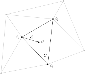
Figure 1: We visualise the construction of the local coordinates $\vec{\alpha}$ of a gauge group element $U\notin\mathcal{D}$ found in 2-simplex (a triangle) $C$ of the triangulation for the simpler two dimensional case. $i_{0}$ is arbitrarily chosen as the origin of the local coordinate system. From there we can then calculate the rotation angles $\vec{\alpha}$ by using eq. 12.

A sketch of this construction for the two dimensional case can be found in fig. 1. We can then use $\vec{\alpha}$ to approximate $f(U)$ within $C$ as

$$f(U)=\tilde{f}(i_{0})+\vec{\nabla}f_{C}\cdot\vec{\alpha}+\mathcal{O}(\alpha^{2})\,,$$ (13)

with $\vec{\nabla}f_{C}$ corresponding to the covariant derivative in $C$ we want to compute. In order to reproduce the function values at the vertices $i_{1,2,3}$ with local coordinates $\vec{\alpha}_{1,2,3}$, $\vec{\nabla}f_{C}$ needs to fulfil the linear equation

$$\begin{pmatrix}\vec{\alpha}^{T}_{1}\\ \vec{\alpha}^{T}_{2}\\ \vec{\alpha}^{T}_{3}\end{pmatrix}\vec{\nabla}f_{C}=\begin{pmatrix}\tilde{f}(i_{1})-\tilde{f}(i_{0})\\ \tilde{f}(i_{2})-\tilde{f}(i_{0})\\ \tilde{f}(i_{3})-\tilde{f}(i_{0})\end{pmatrix}.$$ (14)

For the special case of the basis function $\tilde{f}=\phi_{i}$ only simplices containing $i$ will have a non trivial covariant derivative. As seen in fig. 2 (again for the two dimensional case) it will be pointing in the direction of the normal vector of the face opposite to the vertex $i$.

Similarly, for $R_{c}$ a right $\vec{\nabla}$ can be constructed by introducing coordinates from

$$U=D_{i_{0}}\exp\left(\mathrm{i}\vec{\alpha}\cdot\vec{t}\,\right)$$ (15)

instead of eq. 12 followed by the same steps as above.

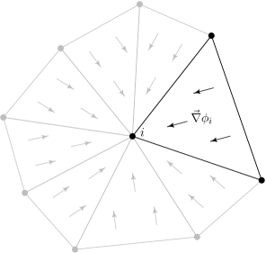
Figure 2: The direction $\vec{\nabla}\phi_{i}$ in the simplices connected to vertex $i$ for a two dimensional example. As can be seen the covariant derivative is orthogonal to the side of the triangle opposing $i$. Its magnitude will be the inverse of the distance to said side.

A good approximation of the covariant derivative at a vertex $i$ can be obtained by taking a weighted average over all simplices $C$ which have $i$ as one of their vertices:

$$\tilde{\nabla}{f}(i)=\frac{1}{W_{i}}\sum_{\{C\in\,\mathcal{C}|i\in C\}}w_{C}\vec{\nabla}f_{C}$$ (16)

with weights $w_{C}$ and

$$W_{i}=\sum_{\{C\in\,\mathcal{C}|i\in C\}}w_{C}\,.$$ (17)

The weight $w_{C}$ can be calculated in different ways as e.g. presented in Ref. Correa et al. (2011). We consider here weighting by the simplex volume

$$w^{\text{vol}}_{C}=\mathrm{Vol}(C)=\frac{1}{6}\left|\det\left(\vec{\alpha}_{1}\,\vec{\alpha}_{2}\,\vec{\alpha}_{3}\right)\right|\,.$$ (18)

Numerical experiments show that this choice of weights works well. Therefore, we leave investigations of alternative choices for future work. It might regain importance in conjunction with ensuring Gauss’ law.

The matrix elements of the operator $\hat{L}_{c}$ are then calculated as

$$\hat{\vec{L}}_{ij}=\begin{pmatrix}\hat{L}_{1\,ij}\\ \hat{L}_{2\,ij}\\ \hat{L}_{3\,ij}\end{pmatrix}=-\mathrm{i}\tilde{\nabla}\phi_{j}(i)\,.$$ (19)

The same holds for $R_{c}$, the only difference being the different calculation of the local coordinates in eq. 15.

III.2 Construction of the Laplace-Beltrami Operator

As our approximation of the covariant derivative is based on linear interpolation, simply calculating $\sum_{c}L_{c}^{2}$ is unlikely to give good results for the Laplace-Beltrami operator. It requires second order derivatives which are intrinsically ignored in linear approximations. Instead, a common approach is to approximate the operator by making use of Greens identity.

We start from the Laplace equation

$$\Delta u=f$$ (20)

and we first introduce the inner product

$$\begin{split}\langle f,g\rangle\coloneqq\sum_{\{C\in\mathcal{C}\}}\int_{C}\mathrm{d}V\,&f(\exp\left(\mathrm{i}\vec{\alpha}\cdot\vec{t}\,\right)U_{i_{0}})\\ &\qquad g(\exp\left(\mathrm{i}\vec{\alpha}\cdot\vec{t}\,\right)U_{i_{0}})\end{split}$$ (21)

where the integral is carried out over the local coordinates defined in eq. 12 and the integral over the volume is split into the sum of the integrals over simplices. We can project eq. 20 to a basis function $\phi$ defined in eq. 10

$$\langle\Delta u,\phi_{i}\rangle=\langle f,\phi_{i}\rangle\,.$$ (22)

The left hand side can be computed using Green’s theorem

$$\begin{split}\langle\Delta u,\phi_{i}\rangle&=\sum_{\{C\in\mathcal{C}\}}\int_{C}\mathrm{d}V(\Delta u)\phi_{i}\\ &=-\sum_{\{C\in\mathcal{C}\}}\int_{C}\mathrm{d}V(\vec{\nabla}u)\cdot(\vec{\nabla}\phi_{i})\\ &\quad+\sum_{\{C\in\mathcal{C}\}}\int_{\partial C}\mathrm{d}S\,\vec{n}\cdot(\vec{\nabla}u)\phi_{i}\,.\end{split}$$ (23)

Here $\vec{n}$ denotes the normal vector of the simplex $C$. As the normal vectors of the two simplices connected at a given face will oppose each other, the boundary term vanishes, when summing over all simplices. In the next step we are approximating the function $u$ with its projection on the space spanned by the basis functions, i.e. $\tilde{u}=\sum_{j}u_{j}\phi_{j}$ obtaining the matrix equation

$$\begin{split}&\langle\Delta u,\phi_{i}\rangle\approx-\sum_{j}u_{j}\sum_{\{C\in\mathcal{C}\}}\int_{C}\mathrm{d}V(\vec{\nabla}\phi_{j})\cdot(\vec{\nabla}\phi_{i})=S_{ij}u_{j}\,.\end{split}$$ (24)

The gradient of the basis function inside a simplex is a constant and the integral over the volume can be computed explicitly

$$S_{ij}=-\sum_{\{C\in\mathcal{C}|i,j\in C\}}(\vec{\nabla}\phi_{j})\cdot(\vec{\nabla}\phi_{i})\mathrm{Vol}(C)\,.$$ (25)

We approximate the integral on the right-hand side of eq. 21 as a Riemann sum

$$\langle f,\phi_{i}\rangle\approx\sum_{j}f(j)\,v(j)\,\phi_{i}(j)=f(i)\,v(i)\,.$$ (26)

As weights we will use the volumes of the cells of the barycentric dual of the triangulation. These distribute the volume of each simplex equally onto each of its vertices and are thus given by

$$v(i)=\sum_{\{C\in\mathcal{C}|i\in C\}}\frac{\mathrm{Vol}(C)}{4}\,.$$ (27)

Equating eqs. 24 and 26 one obtains

$$S_{ij}u_{j}=v_{i}f_{i}\,.$$ (28)

Thus, the matrix form of $\hat{\vec{L}}^{2}$ can then be calculated as

$$\hat{\vec{L}}^{2}_{ij}=-\frac{1}{v_{i}}S_{ij}.$$ (29)

As the Laplacian is independent of local coordinates, $\hat{\vec{R}}^{2}=\hat{\vec{L}}^{2}$ holds like in the continuum also for the discretised operators. Note that like for the linear operator $\hat{\vec{L}}_{ij}$, the matrix form of the discretised operator $\hat{\vec{L}}^{2}_{ij}$ is still local and sparse, even though we have used a global integral definition for its construction. This will no longer be the case if a higher order integration scheme is adopted in eq. 26, in which case one has to take a matrix $M$ on the right had side of the discretised eq. 20 into account, i.e. $S_{ij}u_{j}=M_{ij}f_{j}$. As a consequence one obtains $\hat{\vec{L}}_{ij}^{2}=-M^{-1}_{ik}S_{kj}$ with $M^{-1}$ a dense matrix.

III.3 Partitionings of SU$(2)$

For convenience we compile here the definitions for the partitionings of SU$(2)$ we are going to use in the following. More details on the first four partitionings can be found in Ref. Hartung et al. (2022). The rotated simple cubical and the rotated face centred partitionings are new compared to Ref. Hartung et al. (2022).

III.3.1 Genz Points

We rely on the isomorphism eq. 5 between $S_{3}$ and SU$(2)$ to define the set of Genz points for given $m\geq 1$ as

$$\begin{split}G_{m}&\coloneqq\left\{\left(s_{0}\sqrt{\frac{j_{0}}{m}},s_{1}\sqrt{\frac{j_{1}}{m}},s_{2}\sqrt{\frac{j_{2}}{m}},s_{3}\sqrt{\frac{j_{3}}{m}}\right)\right.\\ \qquad&\left|\,\sum_{i=0}^{3}j_{i}=m,\;\forall i\in\{0,1,2,3\}:\,s_{i}\in\{\pm 1\},\,j_{i}\in\mathbb{N}\right\}\,.\end{split}$$ (30)

This contains all integer partitions $\{j_{0},\dots,j_{3}\}$ of $m\geq 1$ including all permutations and adding all possible sign combinations.

III.3.2 Linear Partitioning

Very similarly, the linear partitioning is defined as the set of points in $S_{3}$ based on the same isomorphism

$$\begin{split}L_{m}&\coloneqq\left\{\frac{1}{M}\left(s_{0}j_{0},s_{1}j_{1},s_{2}j_{2},s_{3}j_{3}\right)\right.\\ &\left|\,\sum_{i=0}^{3}j_{i}=m,\;\forall i\in\{0,1,2,3\}:\,s_{i}\in\{\pm 1\},\,j_{i}\in\mathbb{N}\right\}\,,\end{split}$$ (31)

with

$$M\coloneqq\sqrt{\sum_{i=0}^{3}j_{i}^{2}}\,.$$ (32)

$M$ takes values $m\geq M\geq\frac{m}{\sqrt{4}}$.

III.3.3 Volleyball Partitioning

A variation of $L_{m}$ is given by the Volleyball partitioning

$$\begin{split}V_{m}&\coloneqq\left\{\frac{1}{M}\left(j_{0},j_{1},j_{2},j_{3}\right)\right.\\ &\left|\,(j_{0},\dots,j_{3})\in\left\{\text{all perm. of }\left(\pm\frac{m}{2},a_{1},\dots,a_{3}\right)\right\},\right.\\ &\left.\qquad\,a_{i}\in\{-\frac{m}{2},-\frac{m}{2}+1,\dots,\frac{m}{2}\}\vphantom{\frac{1}{M}}\right\}\end{split}$$ (33)

with $M$ defined in eq. 32, which takes values $m\leq M\leq\sqrt{4}\,m$. Additionally, the corners of the hypercube, in four dimensions also called $C_{8}$, form

$$V_{0} \coloneqq\left\{\frac{1}{\sqrt{4}}\left(s_{0},\dots,s_{3}\right)|\,s_{i}\in\{\pm 1\}\right\}\,,$$ (34)

which is responsible for the name.

III.3.4 Fibonacci Partitioning

For a Fibonacci like lattice on $S_{3}$ we first generate a lattice the unit cube $[0,1)^{3}$ defined by

$$\Lambda_{n}^{\textrm{Fib}} =\left\{t_{m}\middle|0\leq m<n,\,\,m\in\mathbb{N}\right\}$$

$$t_{m} =\begin{pmatrix}t_{m}^{1}\\ t_{m}^{2}\\ t_{m}^{k}\end{pmatrix}=\begin{pmatrix}\frac{m}{n}&\\ a_{1}\,m\quad&\mathrm{mod}\quad 1\\ a_{2}\,m\quad&\mathrm{mod}\quad 1\\ \end{pmatrix}$$

with

$$\frac{a_{i}}{a_{j}}\notin\mathbb{Q}\quad\textrm{for}\quad i\neq j\textrm{,}$$ (35)

where $\mathbb{Q}$ denotes the field of rational numbers. In Ref. Hartung et al. (2022) we have chosen $a_{1}=\sqrt{2}$ and $a_{2}=\sqrt{3}$. The set of points $\Lambda_{n}$ can then be mapped to arbitrary manifolds, such as $S_{3}$. In order to maintain a uniform density of points, this map needs to volume preserving. In spherical coordinates, defined by

$$\ z(\psi,\theta,\phi)=\left(\begin{array}[]{l}\cos\psi\\ \sin\psi\cos\theta\\ \sin\psi\sin\theta\cos\phi\\ \sin\psi\sin\theta\sin\phi\end{array}\right)$$ (36)

it can be implemented by the functions

$$\begin{split}\psi(t_{m})&=\Phi_{1}(t^{1}_{m})\,,\\ \theta(t_{m})&=\cos^{-1}\left(1-2\,t^{2}_{m}\right)\\ \text{and}\qquad\phi(t_{m})&=2\pi t^{3}_{m}\,,\end{split}$$ (37)

where the function $\Phi_{1}(\psi)$ is defined via its inverse

$$\Phi_{1}^{-1}(\psi)=\frac{1}{\pi}\left(\psi-\frac{1}{2}\sin(2\psi)\right)\,.$$ (38)

III.3.5 Other Uniform Partitionings

Finally we can also use the functions defined in eq. 37 to map other uniform point sets from the unit cube to the sphere. An obvious choice would be the simple cubic lattice defined by Hahn (2001)

$$\Lambda_{n}^{\textrm{SC}}=\left\{\vec{x}\in[0,1)^{3}\,\middle|\,\vec{x}=d_{\textrm{SC}}(n)\,\textrm{R}\,\vec{m}\,,\vec{m}\in\mathbb{Z}^{3}\right\}$$ (39)

with a rotation matrix $\textrm{R}\in\textrm{SO}(3)$. Here $d_{\textrm{SC}}(n)$ denotes the lattice spacing needed to fit $n$ points into the unit cube

$$d_{\textrm{SC}}(n)=n^{-1/3}\,.$$

The number of sites found inside the cube will be close to $n$. In general we however still expect a small difference between $n$ and $N\equiv|\Lambda_{n}^{\textrm{SC}}|$. While this is no issue for our application, an exact matching can in principle be achieved by additionally implementing and tuning a translational offset between the unit cube and the lattice.

The rotation matrix R is used to achieve misalignment of the lattice planes and the faces of the unit cube. This is required to ensure that lattice sites cross the cube boundary individually with varying lattice spacing. Thus no entire plane of lattice sites is found just in or outside the cube. For the cubical lattice successive rotations by an angle of $\pi/8$ around $\hat{e}_{1}$, $\hat{e}_{2}$ and $\hat{e}_{3}$ seem to work well.

To maximise the distance between points we also consider the face centred cubic lattice given by Hahn (2001)

$$\begin{split}\Lambda_{n}^{\textrm{FCC}}=\left\{\vec{x}\in[0,1)^{3}\,\middle|\,\vec{x}=\frac{d_{\textrm{FCC}}(n)}{\sqrt{2}}\,\textrm{R}\,\begin{pmatrix}m_{1}+m_{3}\\ m_{2}+m_{3}\\ m_{1}+m_{2}\end{pmatrix},\right.\\ \left.\vec{m}\in\mathbb{Z}^{3}\right\}\,.\end{split}$$ (40)

The lattice spacing for $n$ points is here given by

$$d_{\textrm{FCC}}(n)=\sqrt[6]{2}\,n^{-1/3}$$ (41)

and maximal as proved in Ref. Hales (2006). $R$ is kept from the simple cubical lattice. In the following we will refer to these partitionings as the rotated simple cubical (RSC) and the rotated face centred cubical (RFCC) partitioning respectively.

III.4 Operator Convergence

The discretised Laplace-Beltrami operator directly enters the Hamiltonian. Thus, we have to make sure that first of all the spectrum of the discretised operator converges to the corresponding continuum spectrum. From the original publication by Kogut and Susskind Kogut and Susskind (1975) the spectrum should be determined by main angular momentum quantum number $J$ and two independent magnetic quantum numbers $m_{L}$ and $m_{R}$ with $J\geq m_{L},m_{R}\geq 0$. The two magnetic quantum numbers emerge because every link connects to two lattice sites with independent gauge transformations (or left and right gauge transformations). Therefore, the continuum spectrum is given by

$$\mathcal{S}\ =\ \{J(J+2)\,,\quad J=0,1,2,\ldots\}$$ (42)

with multiplicity $(J+1)^{2}$. We note that the eigenvalues are usually written as $\lambda=j(j+1)$ with $j=0,1/2,1,...$ Kogut and Susskind (1975). The form given above is obtained through rescaling by a factor $4$ and identifying $J=2j$. Then, it matches the spectrum eq. 42 of the Laplace-Beltrami operator on $S_{3}$ discussed above.

In addition to the spectrum we also require that the correct states, i.e. the wave functions, are obtained in the continuum limit. In order to show this we resort to the concept of convergence in the resolvent sense. Let $\mathcal{R}$ be the set of resolvents of $-\Delta$. In our case $\mathcal{R}=\mathbb{C}\setminus\mathcal{S}$, because then with any given $\rho\in\mathcal{R}$ the inverse of $(\rho-\Delta)$ exists and is bounded from above. Then, we need to show that

$$\lim_{m\to\infty}\|(\rho-\Delta)^{-1}-(\rho-\Delta_{\mathcal{D}_{m}})^{-1}\|\ =\ 0\,,$$ (43)

with $\lim_{m\to\infty}\mathcal{D}_{m}=S_{3}$. Although, the functional analytic convergence analysis of the approximation is shown in appendix A, the analysis in appendix A only implies convergence of the spectrum without any further detail on the rate of convergence. At this point, we will therefore check eq. 43 numerically because the convergence of the spectrum can be estimated against the convergence of resolvents using holomorphic functional calculus for the spectral projectors Hartung (2015).

To do so, we first introduce the eigenfunctions $Y_{J,l_{1},l_{2}}$ of $-\Delta$ in the continuum. They are given by the spherical harmonics in four dimensions Erdélyi et al. (1953).

Note that $J$ is the same as above and the eigenvalues of the continuum $\Delta$ are independently of $l_{1}$ and $l_{2}$ given by $\lambda=J(J+2)$. The $l_{1,2}$ are not identical with the magnetic quantum numbers $m_{L,R}$, however. Instead, the obey the condition $J\geq l_{1}\geq|l_{2}|$. It can readily be checked that this condition leads to the same multiplicity $(J+1)^{2}$ as above.

The spherical harmonics can be expressed in terms of the spherical coordinates introduced in eq. 36 as

$$Y_{J,l_{1},l_{2}}=\frac{\mathrm{e}^{il_{2}\varphi}}{\sqrt{2}}\,{}_{2}\overline{P}^{|l_{2}|}_{l_{1}}(\theta)\,{}_{3}\overline{P}^{l_{1}}_{J}(\psi)\,,$$ (44)

where

$$\begin{split}{}_{n}\overline{P}^{l}_{L}(\zeta)=\sqrt{\frac{2L+n-1}{2}\frac{(L+l+n-2)!}{(L-l)!}}&\\ \times\frac{1}{(\sin\zeta)^{(n-2)/2}}\,P^{-\left(l+\frac{n-2}{2}\right)}_{L+\frac{n-2}{2}}&(\cos\zeta)\,.\end{split}$$ (45)

$P^{-\mu}_{\nu}(x)$ here denote the Legendre functions of first kind and are given in terms of the hyper-geometric function ${}_{2}F_{1}$ as

$$\begin{split}P^{-\mu}_{\nu}(x)=\frac{1}{\Gamma(1+\mu)}&\left(\frac{1-x}{1+x}\right)^{\mu/2}\\ {}_{2}F_{1}&\left(-\nu,\nu+1;1+\mu;\frac{1-x}{2}\right).\end{split}$$ (46)

Similarly to their famous counterparts on $S_{2}$, these form an orthonormal basis of the square integrable functions on $S_{3}$. Thus we can express the discretised operator $\Delta_{\mathcal{D}_{m}}$ in this basis by evaluating

$$\begin{split}\langle Y_{J,l_{1},l_{2}},\Delta_{\mathcal{D}_{m}}Y_{J^{\prime},l_{1}^{\prime},l_{2}^{\prime}}\rangle&=\\ \int_{S_{3}}\mathrm{d}V\,&Y_{J,l_{1},l_{2}}\,\Delta_{\mathcal{D}_{m}}Y_{J^{\prime},l_{1}^{\prime},l_{2}^{\prime}}\,.\end{split}$$ (47)

Similarly to eq. 26, we can approximate this integral numerically by evaluating the spherical harmonics at the vertices of $\mathcal{D}_{m}$ and weighting them with the corresponding barycentric cell volume $v(j)$.

If we then implement an upper limit for $J$ by imposing $J<J^{\max}$ we can finally evaluate and check eq. 43. Such a truncation is acceptable, as bigger $J$ correspond to bigger eigenvalues $\lambda=J(J+2)$ leading to decreasing contributions to the inverse operator $(\rho-\Delta)^{-1}$.

As the operator norm $\|\cdot\|$ of an operator $O$ we choose

$$\|O\|=\sqrt{\lambda_{\max}}$$ (48)

where $\lambda_{\max}$ denotes the biggest eigenvalue of $O^{\dagger}O$.

IV Numerical Experiments

In the following, we benchmark the performance of several representative partitionings as applied to different observables. A complete list including all the partitionings we considered for this work can be found in appendix B.

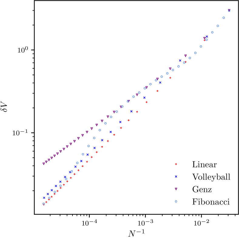
Figure 3: The volume of $S_{3}$ minus the sum of the barycentric cell volumes as a function of $1/N$ in a double log plot. Here, $N$ is the number of points in the partitioning. We compare Fibonacci, Genz, Linear and Volleyball partitionings as indicated in the legend.

IV.1 Volume Convergence

In section III we have shown how to construct the Laplace-Beltrami operator based on a triangulation procedure in $S_{3}$ based on the partitioning. For this we have used the barycentric cell volumes $v(j)$ according to eq. 27. The sum of all $v(j)$ approximates the volume of $S_{3}$, and by increasing the number of points in the partitioning we expect convergence towards Vol$(S_{3})$.

The speed of convergence will certainly depend on the actual partitioning, and we expect this in turn to influence the approximation of the Laplace-Beltrami operator. This is in particular so because we have used Greens theorem neglecting the fact that we only approximate $S_{3}$.

In fig. 3 we plot

$$\delta V\ =\ \mathrm{Vol}(S_{3})-\sum_{j}v(j)$$

as a function of $1/N$ for different partitionings in a double logarithmic plot, where we recall that $N$ is the number of elements in the respective partitioning. For the Genz, the Linear and the Volleyball partitionings we observe that the missing volume $\delta V$ is proportional to $N^{-y}$ with $y\approx 2/3$ for Linear and Volleyball partitionings and $y\approx 1/2$ for the Genz points.

Since the mean distance between two points is roughly $N^{-1/3}$, we conclude that convergence towards $S_{3}$ appears to be quadratic in the mean distance for the Linear and the Volleyball partitioning. For the Genz points on the other hand convergence is proportional to the mean distance to the power of $3/2$, and thus significantly slower. We recall from Hartung et al. (2022) that the distance between neighbouring points is $1/m$ for the Linear partitioning $L_{m}$ mostly independent of the direction, whereas it is between $1/m$ and $\sqrt{2/m}$ for the Genz partitioning $G_{m}$ depending on the direction and the point itself. In particular, the weights of the different points (derived from the associated volume) differ by up to a factor $m^{3/2}$ for $G_{m}$, while the corresponding weight factor for $L_{m}$ is independent of $m$. Thus, Genz points are significantly less isotropically distributed on $S_{3}$, which is responsible for the slower convergence.

The Fibonacci partitioning with $a_{1}=\sqrt{2}$ and $a_{2}=\sqrt{3}$ fixed for all $N$ shows an irregular convergence behaviour: for small $N$ it seems to be similar to the Linear partitioning, then it appears to converge like the Genz points for intermediate $N$-values, but gets in line again with the Linear partitioning for large $N$. Similar behaviour is also observed for other choices for $a_{1}$ and $a_{2}$, only the location of the bump changes.

The reason for this is the following: for a poor choice of the coefficients $a_{1}$ and $a_{2}$ the modulo operation in $t_{m}^{2}$ and $t_{m}^{3}$ can lead to an almost periodic behaviour, such that $t_{m}^{2/3}\approx t_{m+p}^{2/3}$. If the period $p$ is small, this means that the points $t_{m}$ and $t_{m+p}$ end up close together in the cube and on $S_{3}$. Having multiple lattice sites in almost the same spot will do little to improve the quality of our Riemann sum and thus leads to the slowing down in convergence. The return to the convergence rate of the linear and Volleyball partitionings towards larger $N$ is observed, because eq. 35 ensures that $t_{m}^{2/3}\neq t_{m+p}^{2/3}$. Their non-zero difference then becomes more and more significant with finer lattice spacing, and thus eventually removes the periodicity in the coordinates.

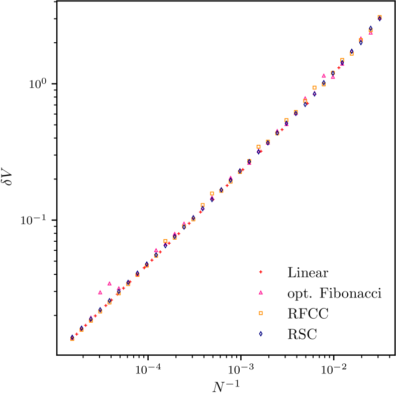
Figure 4: Like fig. 3, but comparing the original Fibonacci partitioning with the optimised one and the RFCC and RSC partitionings.

In order to overcome this irregular convergence pattern of the original Fibonacci partitioning, we choose $a_{1}$ and $a_{2}$ separately for each $N$. The distance of a potential close neighbour with period $p$ can be calculated as

$$\begin{split}\delta_{N}(p,a_{1},a_{2})&=\left[(p/N)^{2}+(pa_{1}\mod 1)^{2}\right.\\ &\qquad\qquad\qquad\left.+(pa_{2}\mod 1)^{2}\right]^{1/2}\,.\end{split}$$ (49)

An upper bound for $p$ is given by

$$\frac{p}{N}<d_{\textrm{FCC}}(N)$$

as the face centred cubical packing maximises the distance between lattice points. Thus we can predict the distance to the closest neighbour for two coefficients $a_{1}$ and $a_{2}$ by evaluating

$$d_{\textrm{Fib}}(N,a_{1},a_{2})=\min\left(\left\{\delta_{N}(p,a_{1},a_{2})\,\middle|\,p\in\mathbb{N}\setminus\{0\}\right\}\right)\,.$$ (50)

With this we can simply iterate over a suitable set of coefficients $a_{1/2}$ until the desired minimum distance is reached. In our implementation we iterated over the square roots of the prime numbers until

$$\frac{d_{\textrm{Fib}}(n,a_{1},a_{2})}{d_{\textrm{FCC}}(n)}\geq 0.95$$ (51)

was fulfilled.

The volume convergence of the original and the such optimised Fibonacci partitionings are compared in fig. 4. We observe that the irregularities are mostly gone in the optimised version. However, since $a_{1}$ and $a_{2}$ parameters are optimised for each $N$, one can expect a uniform convergence rate, but the amplitude might still depend on $N$, which is what we see in the form of outliers. In the following we, therefore, use the Fibonacci partitioning with optimised values for $a_{1}$ and $a_{2}$ only.

This remaining irregularity can be cured by using the RFCC or the RSC partitionings, as also shown in fig. 4. The smallest overall deviations from the volume of $S_{3}$ are actually observed for the RFCC partitioning, but the RSC does not perform significantly worse.

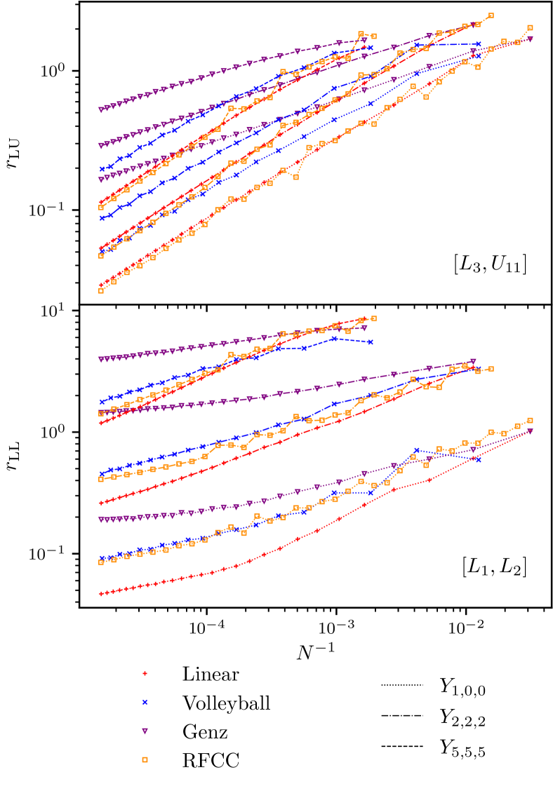
Figure 5: We show $r_{\mathrm{LU}}$ (upper panel) and $r_{\mathrm{LL}}$ (lower panel) as a function of $1/N$ for three different spherical harmonics in a double log plot. We compare Linear, Volleyball, Genz and RFCC partitionings.

IV.2 Commutation Relations

With the above definitions of $\hat{L}$ and $\hat{R}$ it is ensured that if applied to a constant vector one obtains zero. Much like in the one dimensional case of a finite difference operator, we expect $\hat{L}$ and $\hat{R}$ to work best if applied to slowly varying vectors in the algebra. Thus we choose some of the lower lying spherical harmonics $Y_{J,l_{1},l_{2}}$ defined in eq. 44 as test functions. For each harmonic we can compute the corresponding error vector

$$w\ =\ \left([L_{a},U_{jl}]-(t_{a})_{ji}U_{il}\right)\cdot Y_{J,l_{1},l_{2}}$$ (52)

and then the mean deviation weighted by barycentric cell volume $v(i)$ as

$$r_{\mathrm{LU}}\ =\ \sum_{i}v(i)\,|w_{i}|\,.$$ (53)

Likewise, we define

$$u\ =\ \left([L_{a},L_{b}]\ +\ 2\mathrm{i}\,\epsilon_{abc}\,L_{c}\right)\cdot Y_{J,l_{1},l_{2}}\,,$$ (54)

with the appropriate structure constant $f_{abc}$ for SU$(2)$, and

$$r_{\mathrm{LL}}\ =\ \sum_{i}v(i)\,|u_{i}|\,.$$ (55)

In fig. 5 we plot $r_{\mathrm{LU}}$ and $r_{\mathrm{LL}}$ for exemplary combinations of indices $j$ and $l$ as a function of $1/N$. Results are shown for the different partitionings of SU$(2)$ and different spherical harmonics.

We observe that $r_{\mathrm{LU}}$ approaches zero with increasing $N$. The convergence rate appears to be depending on the partitioning used: while Genz points seem to converge the slowest, the Linear and RFCC partitionings work best in this respect. As expected the deviations increase when using faster oscillating harmonics.

For $r_{\mathrm{LL}}$, and thus the deviations from the expected behaviour in the commutator of $L$ with itself, the picture is less clear. We again see a decrease in $r_{\mathrm{LL}}$ with increasing $N$, however, the convergence rate appears slower and the scaling region might set in only at larger $N$ compared to $r_{\mathrm{LU}}$.

Interestingly, the Linear partitioning shows the fastest convergence for $r_{\mathrm{LL}}$ compared to all the other partitionings investigated here.

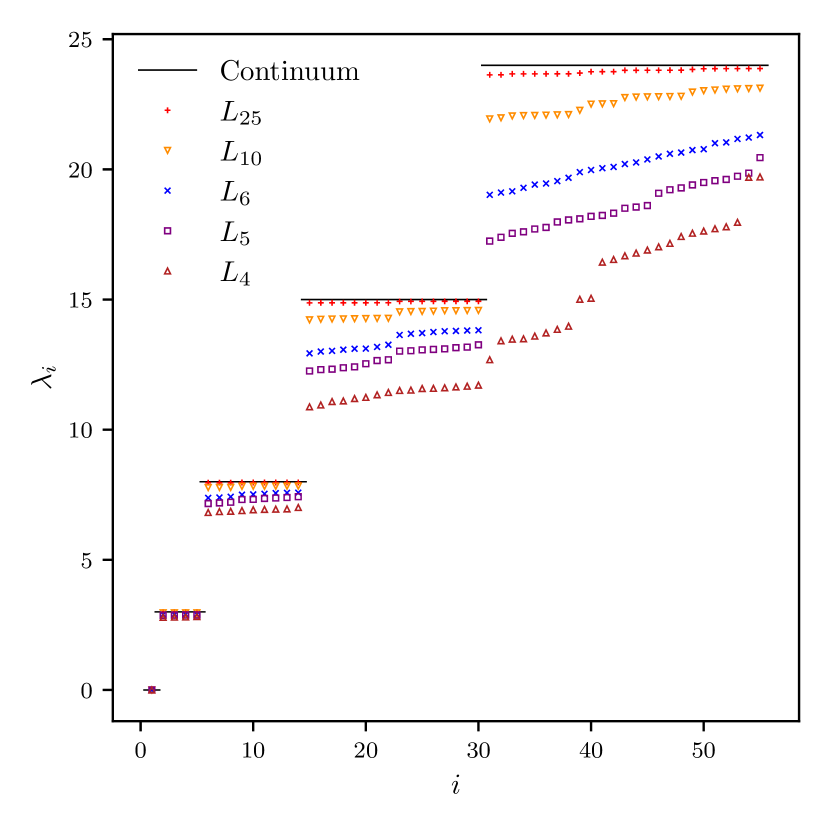
Figure 6: We show the lowest 60 eigenvalues of the discretised Laplace-Beltrami operator for the Linear partitionings $L_{m}$ with $m=4,5,6,10$ and $m=25$. The solid lines corresponds to the expected continuum values from eq. 42.

IV.3 Spectrum in the Free Theory

We compute the spectrum of the discretised Laplace-Beltrami operator $-\Delta_{\mathcal{D}_{m}}$ for different partitionings $\mathcal{D}$ and values of $m$ numerically. We note that the lowest eigenvalue $\lambda_{1}=0$ per construction, and therefore we are going to mostly exclude $\lambda_{1}$ from the following discussion.

For the linear partitioning we show the 60 lowest eigenvalues $\lambda_{i}$ in fig. 6. While the different point styles distinguish values of $m$ from $4$ to $25$, the line indicates the continuum spectrum from eq. 42. It is clearly visible that with increasing $m$ the spectrum of $-\Delta_{L_{m}}$ converges towards the continuum spectrum with the correct multiplicity.

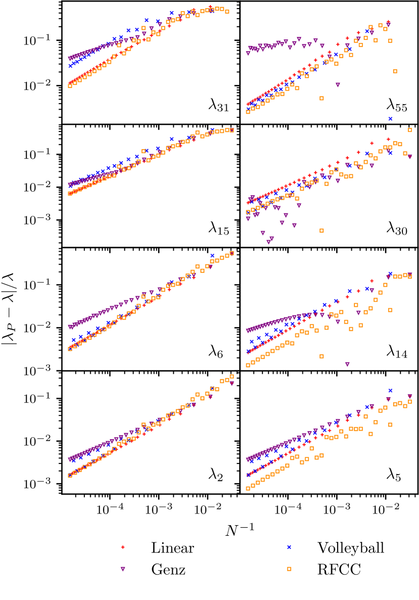
Figure 7: We plot $|\lambda_{\mathrm{P}}-\lambda|/\lambda$ as a function of $1/N$ for the Volleyball, the Linear, the RFCC and the Genz partitionings for the eigenvalues $\lambda_{i}$ with $i=2,5,6,14,15,30,31,55$.

In fig. 7 we show the convergence for different eigenvalues $\lambda_{\mathrm{P}}$ of the discretised Laplace-Beltrami operator separately. We plot the relative deviation from the expected continuum value $\lambda$

$$\frac{|\lambda_{\mathrm{P}}-\lambda|}{\lambda}$$

as a function of $1/N$ for different eigenvalues $\lambda_{k}$ with $k=2,5,6,14,15,30,31,55$. Note that we order the eigenvalues such that $\lambda_{i}\leq\lambda_{i+1}$. Our choices for $i$, therefore, correspond to the first and the last eigenvalue in a multiplet. We observe convergence towards the expected continuum value for all the eigenvalues we investigated and all the partitionings.

The most regular and smooth convergence pattern is observed for the linear partitioning. The Volleyball partitioning behaves similarly, but with some dependence on the actual value of $N$. The convergence rate of the RFCC partitioning falls in line with the one of the Linear partitioning, but with somewhat smaller amplitude.

The Genz partitioning seems to be also converging, however, with a visibly slower convergence rate than the other partitionings towards large $N$-values. In particular for the last eigenvalues of a given multiplet we also observe sign changes in $\lambda_{\mathrm{P}}-\lambda$.

Empirically, the convergence rates appear to be independent of the index $i$ and very similar to the rates of convergence of the volume.

IV.4 Operator Convergence

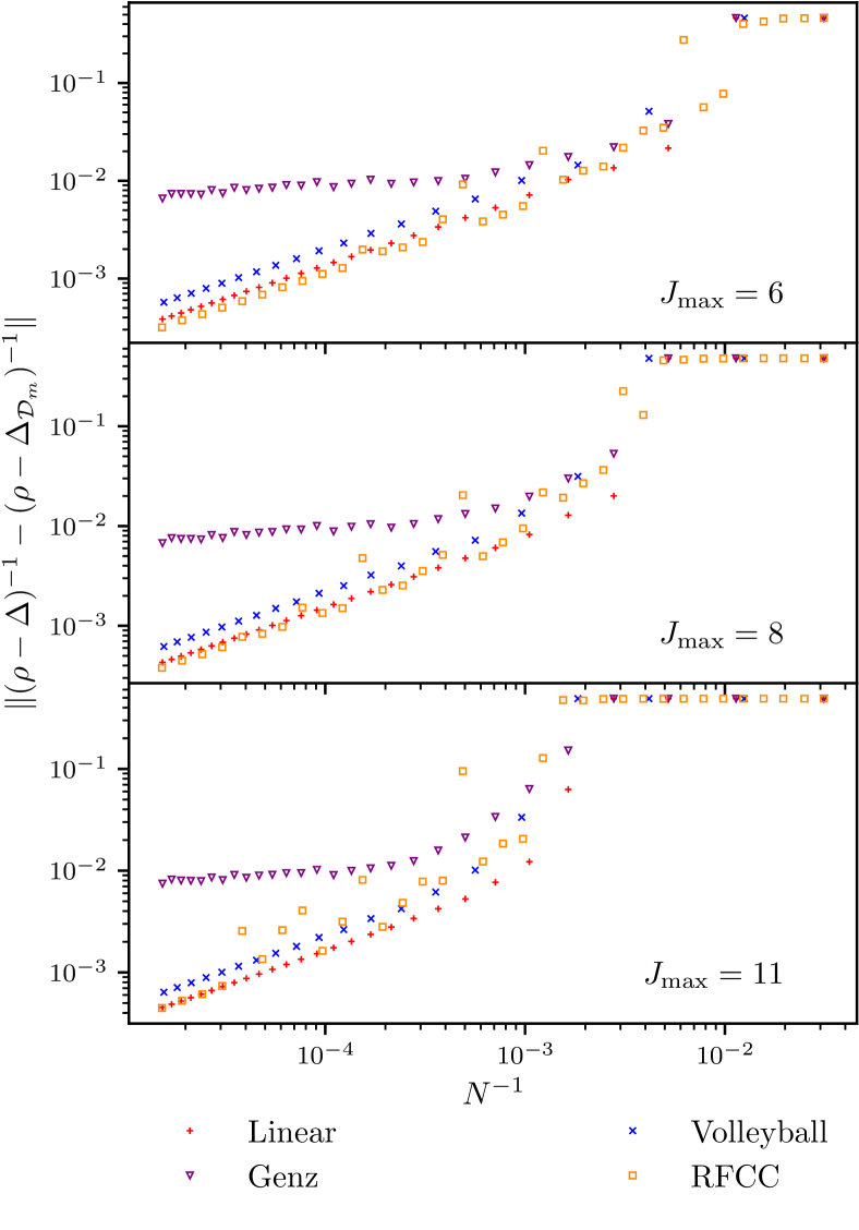
Figure 8: We plot $\|(\rho-\Delta)^{-1}-(\rho-\Delta_{\mathcal{D}_{m}})^{-1}\|$ as a function of $1/N$ evaluated on different sets of eigenfunctions corresponding to $J_{\mathrm{max}}=6$, $J_{\mathrm{max}}=8$ and $J_{\mathrm{max}}=11$ with $\rho=-2$.

Finally, we discuss the operator convergence by checking eq. 43 numerically. For this we pick a value from the resolvent set of $\rho=-2$. Other $\rho$-values lead to similar and qualitatively equivalent results.

In fig. 8 we plot

$$\|(\rho-\Delta)^{-1}-(\rho-\Delta_{\mathcal{D}_{m}(N)})^{-1}\|$$ (56)

as a function of $1/N$ for $\rho=-2$. As discussed in section III.4, we evaluate eq. 56 using a finite subset of the spherical harmonics $Y_{J,l_{1},l_{2}}$ by imposing $J<J_{\mathrm{max}}$. The three different $J_{\mathrm{max}}$-values are $J_{\mathrm{max}}=6$, $J_{\mathrm{max}}=8$ and $J_{\mathrm{max}}=11$.

Concentrating on the uppermost panel for $J_{\mathrm{max}}=6$ to start with, we observe gap convergence for all partitionings shown. The convergence rate is proportional to $N^{-z}$ with $z\approx 0.7$ for all partitionings apart from Genz. For the Genz partitioning the convergence is very slow with $z\approx 0.1$. This picture remains the same for large $N$-values for the two other $J_{\mathrm{max}}$-values.

For $J_{\mathrm{max}}=8$ and $J_{\mathrm{max}}=11$ another feature becomes visible: for $N\to 0$ the gap plateaus at a value of $1/|\rho|$. At the corresponding values of $N$ there are not sufficiently many points in the partitioning to resolve all the $Y_{J,l_{1},l_{2}}$.

V Discussion

There are a few points that deserve discussion. First, the results from the previous section indicate that the points in a partitioning should be as uniformly distributed as possible: the main difference between the Genz $G_{m}$ and the Linear $L_{m}$ partitionings is that in the Genz set points are denser around the poles. This leads to larger deviations from the mean distance for $G_{m}$ compared to $L_{m}$ at fixed $m$, which in turn means slower convergence to the volume of $S_{3}$. This conclusion is strongly supported by the comparison of original Fibonacci and optimised Fibonacci partitioning, where the difference in convergence can be clearly traced back to the non-uniformity in the original Fibonacci version for certain values of $N$. For additional results supporting this conclusion we refer to appendix B.

Since we define the Laplace-Beltrami operator via an integral relation eq. 29, the aforementioned effects from non-uniformity are expected to also influence the spectrum of the discretised operator as well as the gap convergence. This explains the slower convergence rates observed for the Genz partitioning for most of the investigated quantities.

In addition, we observe plateaus in the gap in fig. 8 for small values of $N$. The extent of the plateaus depends on $J_{\mathrm{max}}$. They originate from a sufficiently large $N$ being required to resolve all the states up to a given $J_{\mathrm{max}}$. More specifically, $J$ corresponds to an (angular) momentum. The highest momentum $J_{\text{max}}$ that can be resolved on a lattice, is dictated by the inverse lattice spacing. Put differently, the lattice discretisation acts as an ultraviolet cutoff. Since the lattice spacing is proportional to $N^{-1/3}$, the plateaus are expected for $N\lesssim J_{\text{max}}^{3}$. This is well compatible with fig. 8.

VI Conclusion and Outlook

In this paper we have shown how to discretise the electric part in the Hamiltonian eq. 1 for the gauge group SU$(2)$, when the basis is chosen such that the gauge field operators $\hat{U}$ are diagonal. It turns out that the canonical momentum operators $\hat{L}$ and $\hat{R}$ can be constructed by discretising the corresponding Lie derivatives based on a triangulated partitioning of SU$(2)$. Mostly independently on the choice of the partitioning the such constructed operators fulfil the fundamental commutation relations up to discretisation effects. However, when it comes to reproducing the free spectrum of the theory, it is not sufficient to insert these $\hat{L}$ and $\hat{R}$ squared into the Hamiltonian.

It is rather necessary to construct a discrete version of the electric part in the Hamiltonian directly by realising that it corresponds to the Laplace-Beltrami operator on $S_{3}$. This operator can be discretised by means known from finite element methods.

Then, our results show that with sufficiently uniform partitionings the low lying eigenvalues of the discretised Laplace-Beltrami operator converge towards their continuum counterparts. The larger the number of points $N$ in the partitioning, the more eigenvalues can be resolved. Likewise, the continuum wave functions are reproduced with $N\to\infty$. Thus, we conclude that the discretised free Hamiltonian reproduces the free theory up to discretisation effects. The size of these artefacts can be reduced arbitrarily by increasing $N$.

In the future we will investigate the SU$(2)$ discretisation proposed in this paper beyond the free theory. Moreover, the implementation of Gauss’ law and the consequences of the breaking of the fundamental commutation relations (albeit only by discretisation effects) will be important to understand.

Appendix A Functional analytic point of view on convergence

A.1 Domain of the discretized derivative and Laplacian

We are generally looking for a discretisation of the Laplace-Beltrami in $L_{2}(\mathrm{SU}(2))$. However the discretised derivative $\nabla_{P}$ – as constructed following section III.1 using a triangulated partition $P$ of $\mathrm{SU}(2)$ – requires point-evaluations on the vertices of the partitioning $P$. Hence, we can only a priori define $\nabla_{P}$ on functions in $C(\mathrm{SU}(2))$, and then need to consider the $L_{2}(\mathrm{SU}(2))$ extension of the thus defined $\nabla_{P}|_{C(\mathrm{SU}(2))}$.

Using the Sobolev Embedding for compact manifolds without boundary we obtain the (tightest) embeddings

$$\forall k\geq 2:\ W_{2}^{k}(\mathrm{SU}(2))\subseteq C^{k-2,\frac{1}{2}}(\mathrm{SU}(2)).$$ (57)

In particular, this implies that we can define $\nabla_{P}|_{W_{2}^{2}(\mathrm{SU}(2))}$ using the point-evaluation formula. A priori this means that $\nabla_{P}|_{W_{2}^{2}(\mathrm{SU}(2))}$ maps $W_{2}^{2}(\mathrm{SU}(2))$ into $L_{2}(\mathrm{SU}(2))$ instead of the expected $W_{2}^{1}(\mathrm{SU}(2))$. It is now important to note that, in local coordinates, difference quotients $D_{i}^{h}$ with step size $h$ in direction $i$ satisfy $\left\lVert{D_{i}^{h}u}\right\lVert_{L_{p}(\Omega^{\prime})}\leq\left\lVert{D_{i}u}\right\lVert_{L_{p}(\Omega)}$ for $\Omega^{\prime}\Subset\Omega$ provided $h$ is sufficiently small. Lifting this to $\mathrm{SU}(2)$ means that $\nabla_{P}|_{W_{2}^{2}(\mathrm{SU}(2))}$ is relatively bounded by $\nabla|_{W_{2}^{2}(\mathrm{SU}(2))}$, i.e., $\nabla_{P}|_{W_{2}^{2}(\mathrm{SU}(2))}$ in fact maps $W_{2}^{2}(\mathrm{SU}(2))$ into $W_{2}^{1}(\mathrm{SU}(2))$ as expected and can be uniquely extended to the operator $\nabla_{P}:\ W_{2}^{1}(\mathrm{SU}(2))\to L_{2}(\mathrm{SU}(2))$.

Finally, this implies that the discretised Laplace $\Delta_{P}$ defined as the operator associated with the symmetric form $\tau(x,y)=\langle\nabla_{P}x,\nabla_{P}y\rangle$ is a well-defined map $\Delta_{P}:\ W_{2}^{2}(\mathrm{SU}(2))\to L_{2}(\mathrm{SU}(2))$.

A.2 Pointwise Convergence

Further to the discretised gradient $D^{h}$ defined via difference quotients in local coordinates being bounded by the gradient $\nabla$, $D^{h}f\to\nabla f$ holds in $W_{p}^{k-1}(\Omega)$ for any $f\in W_{p}^{k}(\Omega)$. Hence, again lifting this result to $\mathrm{SU}(2)$, we obtain pointwise convergence $\nabla_{P}\to\nabla$ using the net of discretisations with directed set of partitionings $P^{\prime}\preceq P$ if and only if every vertex of $P^{\prime}$ is also a vertex of $P$. This also implies that the discretised Laplace $\Delta_{P}=\nabla_{P}^{*}\nabla_{P}:\ W_{2}^{2}(\mathrm{SU}(2))\to L_{2}(\mathrm{SU}(2))$ converges pointwise to the Laplace $\Delta=\nabla^{*}\nabla:\ W_{2}^{2}(\mathrm{SU}(2))\to L_{2}(\mathrm{SU}(2))$.

Unfortunately, this pointwise convergence is not sufficient for convergence of the spectrum. To obtain the convergence of the spectrum, we need a notion called gap convergence which is equivalent to norm convergence for bounded operators and convergence in norm resolvent sense for closed operators with non-empty resolvent set Kato (1966). Using eq. 43, we have tested the convergence in norm resolvent sense numerically.

A.3 Finite order gap convergence

Let us consider an orthonormal basis $(\psi_{j})_{j\in\mathbb{N}}$ of $L_{2}(\mathrm{SU}(2))$ with $\forall j\in\mathbb{N}:\ \psi_{j}\in W_{2}^{2}(\mathrm{SU}(2))$. Restricting the space $L_{2}(\mathrm{SU}(2))$ and $W_{2}^{2}(\mathrm{SU}(2))$ to the linear span $L_{2}(\mathrm{SU}(2))|_{n}$ (and $W_{2}^{2}(\mathrm{SU}(2))|_{n}$ with the respective topology) of the first $n$ basis vectors induces restricted operators $\Delta_{P}|_{n}$ and $\Delta|_{n}$. For these, we obtain

$$\begin{aligned} &\left\lVert{\Delta_{P}|_{n}-\Delta|_{n}}\right\lVert_{L(W_{2}^{2}(\mathrm{SU}(2))|_{n},L_{2}(\mathrm{SU}(2))|_{n})}\\ =&\sup_{\left\lVert{\varphi}\right\lVert_{W_{2}^{2}(\mathrm{SU}(2))|_{n}}=1}\left\lVert{\Delta_{P}|_{n}\varphi-\Delta|_{n}\varphi}\right\lVert_{L_{2}(\mathrm{SU}(2))|_{n}}\\ =&\sup_{\left\lVert{\sum_{j=1}^{n}\alpha_{j}\psi_{j}}\right\lVert_{W_{2}^{2}|_{n}}=1}\left\lVert{(\Delta_{P}|_{n}-\Delta|_{n})\sum_{j=1}^{n}\alpha_{j}\psi_{j}}\right\lVert_{L_{2}|_{n}}\\ \leq&\sup_{\left\lVert{\sum_{j=1}^{n}\alpha_{j}\psi_{j}}\right\lVert_{W_{2}^{2}|_{n}}}\sum_{j=1}^{n}|\alpha_{j}|\left\lVert{(\Delta_{P}|_{n}-\Delta|_{n})\psi_{j}}\right\lVert_{L_{2}|_{n}}.\end{aligned}$$ (58)

Since $\left\lVert{\cdot}\right\lVert_{W_{2}^{2}(\mathrm{SU}(2))}\geq\left\lVert{\cdot}\right\lVert_{L_{2}(\mathrm{SU}(2))}$ we observe for $\varphi=\sum_{j=1}^{n}\alpha_{j}\psi_{j}\in\partial B_{W_{2}^{2}(\mathrm{SU}(2))|_{n}}$

$$\begin{aligned} \sum_{j=1}^{n}|\alpha_{j}|=&\left\lVert{\alpha}\right\lVert_{\ell_{1}(n)}\leq\sqrt{n}\left\lVert{\alpha}\right\lVert_{\ell_{2}(n)}=\sqrt{n}\left\lVert{\varphi}\right\lVert_{L_{2}}\\ \leq&\sqrt{n}\left\lVert{\varphi}\right\lVert_{W_{2}^{2}}=\sqrt{n}\end{aligned}$$ (59)

and thus

$$\begin{aligned} \left\lVert{\Delta_{P}|_{n}-\Delta|_{n}}\right\lVert\leq&\sqrt{n}\underbrace{\max_{j\leq n}\left\lVert{(\Delta_{P}|_{n}-\Delta|_{n})\psi_{j}}\right\lVert_{L_{2}|_{n}}}_{\to 0\ (P\nearrow)}.\end{aligned}$$ (60)

Since norm convergence and gap convergence are equivalent for bounded operators, we can conclude that the restricted discretised Laplace converges in gap to the restricted continuum Laplace.

A.4 $L_{2}$ with decay

Unfortunately, this gap convergence seems not to extend to all of $L_{2}(\mathrm{SU}(2))$. Instead, we consider a conic submanifold of “$L_{2}$-functions with decay”. A function $\varphi\in L_{2}(\mathrm{SU}(2))$ is an element of $L_{2,0(\beta,\delta)}(\mathrm{SU}(2))$ if and only if for a given orthonormal basis $\beta=(\psi_{j})_{j\in\mathbb{N}}$ of $L_{2}(\mathrm{SU}(2))$ and a decay function $\delta:\ \mathbb{N}\to\mathbb{R}_{>0}$ with $\delta(n)\to 0\ (n\to\infty)$

$$\forall n\in\mathbb{N}:\ \left\lVert{\varphi-\sum_{j=1}^{n}\langle\psi_{j},\varphi\rangle\psi_{j}}\right\lVert_{L_{2}(\mathrm{SU}(2))}\leq\delta(n)\left\lVert{\varphi}\right\lVert$$ (61)

holds. In other words, we restrict the space of functions to those whose Fourier modes of order $n$ and higher contribute no more than $\delta(n-1)$ in norm. In this sense, this is similar to a UV cutoff although not quite as strong as still arbitrarily large Fourier modes are allowed, they just cannot have arbitrarily large Fourier coefficients.

For given $n$, we will use the notation

$$\varphi^{\downarrow}= \sum_{j=1}^{n}\langle\psi_{j},\varphi\rangle\psi_{j}\text{ and }\varphi^{\uparrow}=\sum_{j=n+1}^{\infty}\langle\psi_{j},\varphi\rangle\psi_{j}.$$ (62)

We note that this $L_{2,0(\beta,\delta)}(\mathrm{SU}(2))$ is a closed conic submanifold of $L_{2}(\mathrm{SU}(2))$ since for $\varphi\in L_{2,0(\beta,\delta)}(\mathrm{SU}(2))$ and $r>0$ we obtain $r\varphi\in L_{2,0(\beta,\delta)}(\mathrm{SU}(2))$ (conic), and for $\varphi_{k}\in L_{2,0(\beta,\delta)}(\mathrm{SU}(2))$ and $\varphi_{k}\to\varphi$ in $L_{2}(\mathrm{SU}(2))$ we have

$$\begin{aligned} &\left\lVert{\varphi-\sum_{j=1}^{n}\langle\psi_{j},\varphi\rangle\psi_{j}}\right\lVert\\ \leq&\left\lVert{\varphi-\varphi_{k}}\right\lVert+\left\lVert{\varphi_{k}-\sum_{j=1}^{n}\langle\psi_{j},\varphi_{k}\rangle\psi_{j}}\right\lVert\\ &+\left\lVert{\sum_{j=1}^{n}\langle\psi_{j},\varphi_{k}-\varphi\rangle\psi_{j}}\right\lVert\\ \leq&2\underbrace{\left\lVert{\varphi-\varphi_{k}}\right\lVert}_{\to 0}+\underbrace{\left\lVert{\varphi_{k}-\sum_{j=1}^{n}\langle\psi_{j},\varphi_{k}\rangle\psi_{j}}\right\lVert}_{\leq\delta(n)\left\lVert{\varphi_{k}}\right\lVert}\\ \leq&\delta(n)\left\lVert{\varphi_{k}}\right\lVert+o(1)\\ \to&\delta(n)\left\lVert{\varphi}\right\lVert,\end{aligned}$$ (63)

i.e., $L_{2,0(\beta,\delta)}(\mathrm{SU}(2))$ is closed.

A.5 Gap convergence with decay

Unfortunately, $L_{2,0(\beta,\delta)}(\mathrm{SU}(2))$ is not a linear subspace since sums of its elements is in general not elements of $L_{2,0(\beta,\delta)}(\mathrm{SU}(2))$. However, it has the induced topology from $L_{2}(\mathrm{SU}(2))$ and thus the $L(L_{2}(\mathrm{SU}(2)))$ and $L(W_{2}^{2}(\mathrm{SU}(2)),L_{2}(\mathrm{SU}(2)))$ norms computed by restricting the unit sphere of $L_{2}(\mathrm{SU}(2))$ and $W_{2}^{2}(\mathrm{SU}(2))$ respectively are consistent with the operator norms in $L(L_{2,0(\beta,\delta)}(\mathrm{SU}(2)))$ and $L(W^{2}_{2,0(\beta,\delta)}(\mathrm{SU}(2)),L_{2,0(\beta,\delta)}(\mathrm{SU}(2)))$. Here, we denote the restriction to $W^{2}_{2,0(\beta,\delta)}(\mathrm{SU}(2))$ as the set of $L_{2}(\mathrm{SU}(2))$ functions $\varphi$ whose derivatives up to second order are in $L_{2,0(\beta,\delta)}(\mathrm{SU}(2))$ including the condition that derivatives up to second order of $\varphi^{\uparrow}$ are bounded by $\delta$. This is still a closed conic submanifold of $L_{2}(\mathrm{SU}(2))$ and of $W_{2}^{2}(\mathrm{SU}(2))$ using the same argument as in eq. 63 changing only the norm. It should be noted that this requires $\beta$ to be an orthonormal basis that is contained in $W_{2}^{2}(\mathrm{SU}(2))$. In our case, this basis given by the spherical harmonics which are in $W_{2}^{\infty}(\mathrm{SU}(2))$, i.e., this restriction on $\beta$ is irrelevant for the application we are considering.

Let us consider $\varphi\in L_{2,0(\beta,\delta)}(\mathrm{SU}(2))$ such that $\Delta\varphi,\Delta_{P}\varphi\in L_{2,0(\beta,\delta)}(\mathrm{SU}(2))$ and $\left\lVert{\varphi}\right\lVert_{W^{2}_{2}(\mathrm{SU}(2))}=1$. Then, we observe

$$\begin{aligned} \left\lVert{\Delta\varphi-\Delta_{P}\varphi}\right\lVert_{L_{2}}\leq&\left\lVert{(\Delta\varphi^{\downarrow})^{\downarrow}-(\Delta_{P}\varphi^{\downarrow})^{\downarrow}}\right\lVert_{L_{2}}\\ &+\left\lVert{(\Delta\varphi^{\uparrow})^{\downarrow}-(\Delta_{P}\varphi^{\uparrow})^{\downarrow}}\right\lVert_{L_{2}}\\ &+\underbrace{\left\lVert{(\Delta\varphi)^{\uparrow}-(\Delta_{P}\varphi)^{\uparrow}}\right\lVert_{L_{2}}}_{\leq\mathrm{dim}(\mathrm{SU}(2))\delta(n)}\\ \leq&\left\lVert{\Delta|_{n}\varphi^{\downarrow}-\Delta_{P}|_{n}\varphi^{\downarrow}}\right\lVert_{L_{2}}\\ &+\underbrace{\left\lVert{\Delta\varphi^{\uparrow}-\Delta_{P}\varphi^{\uparrow}}\right\lVert_{L_{2}}}_{\leq\mathrm{dim}(\mathrm{SU}(2))\delta(n)}+3\delta(n)\\ \leq&\left\lVert{\Delta|_{n}\varphi^{\downarrow}-\Delta_{P}|_{n}\varphi^{\downarrow}}\right\lVert_{L_{2}}+6\delta(n).\end{aligned}$$ (64)

Using $\delta(n)\to 0$ and the finite order gap convergence result, we conclude that for every $\varepsilon>0$ there exists an $n\in\mathbb{N}$ and a partitioning $P_{0}$ such that every partitioning $P\succeq P_{0}$ such that

$$\delta(n)<\frac{\varepsilon}{12}.$$ (65)

Subsequently, we can find a partitioning $P_{0}$ such that every partitioning $P\succeq P_{0}$ satisfies

$$\left\lVert{\Delta|_{n}-\Delta_{P}|_{n}}\right\lVert_{L(W_{2}^{2}(\mathrm{SU}(2))|_{n},L_{2}(\mathrm{SU}(2))|_{n})}<\frac{\varepsilon}{2}.$$ (66)

With these choices of $n$ and $P_{0}$, we obtain for $P\succeq P_{0}$ (note $\left\lVert{\varphi^{\downarrow}}\right\lVert_{W_{2}^{2}(\mathrm{SU}(2))}\leq\left\lVert{\varphi}\right\lVert_{W^{2}_{2}(\mathrm{SU}(2))}=1$)

$$\begin{aligned} \left\lVert{\Delta\varphi-\Delta_{P}\varphi}\right\lVert_{L_{2}}\leq&\left\lVert{\Delta|_{n}\varphi^{\downarrow}-\Delta_{P}|_{n}\varphi^{\downarrow}}\right\lVert_{L_{2}}+6\delta(n)\\ \leq&\frac{\varepsilon}{2}\left\lVert{\varphi^{\downarrow}}\right\lVert_{W_{2}^{2}}+6\frac{\varepsilon}{12}\\ \leq&\varepsilon.\end{aligned}$$ (67)

Hence,

$$\left\lVert{\Delta-\Delta_{P}}\right\lVert_{L(W_{2,0(\beta,\delta)}^{2}(\mathrm{SU}(2)),L_{2,0(\beta,\delta)}(\mathrm{SU}(2)))}<\varepsilon$$ (68)

shows norm convergence and therefore gap convergence of $\Delta_{P}\to\Delta$ as operators from $W_{2,0(\beta,\delta)}^{2}(\mathrm{SU}(2))$ to $L_{2,0(\beta,\delta)}(\mathrm{SU}(2))$.

Since gap convergence is equivalent convergence in norm-resolvent sense, we obtain that for every $\rho$ in the resolvent set $\mathcal{R}(\Delta)$ of $\Delta$, there exists $P_{0}$ such that for every $P\succeq P_{0}$ we also have $\rho\in\mathcal{R}(\Delta_{P})$ and

$$\left\lVert{(\rho-\Delta_{P})^{-1}-(\rho-\Delta)^{-1}}\right\lVert_{L(L_{2,0(\beta,\delta)},W_{2,0(\beta,\delta)}^{2})}\to 0.$$ (69)

Finally, since the embedding

$$\iota:\ W_{2}^{2}(\mathrm{SU}(2))\hookrightarrow L_{2}(\mathrm{SU}(2))$$ (70)

is bounded with $\left\lVert{\iota}\right\lVert_{L(W_{2}^{2}(\mathrm{SU}(2)),L_{2}(\mathrm{SU}(2)))}\leq 1$, we know that the resolvents $(\rho-\Delta_{P})^{-1}$ and $(\rho-\Delta)^{-1}$ map into $L_{2,0(\beta,\delta)}$ as well and, as maps from $L_{2,0(\beta,\delta)}$ to $L_{2,0(\beta,\delta)}$, can they can be expressed as

$$\iota\circ(\rho-\Delta_{P})^{-1}\text{ and }\iota\circ(\rho-\Delta)^{-1}.$$ (71)

In other words,

$$\left\lVert{(\rho-\Delta_{P})^{-1}-(\rho-\Delta)^{-1}}\right\lVert_{L(L_{2,0(\beta,\delta)},L_{2,0(\beta,\delta)})}$$ (72)

is bounded by

$$\left\lVert{(\rho-\Delta_{P})^{-1}-(\rho-\Delta)^{-1}}\right\lVert_{L(L_{2,0(\beta,\delta)},W_{2,0(\beta,\delta)}^{2})}$$ (73)

which directly implies convergence in norm-resolvent sense for the discretised Laplace in $L_{2,0(\beta,\delta)}(\mathrm{SU}(2))$.

As a final note, while $L_{2}(\mathrm{SU}(2))$ can be written in terms of an inductive limit of $L_{2,0(\beta,\delta)}(\mathrm{SU}(2))$ with an increasing sequence of decay functions $\delta$, the convergence does not seem to lift to the inductive limit because $\varphi_{n}\to\varphi$ in $L_{2}(\mathrm{SU}(2))$ does not seem to imply that $\varphi_{n}$ has to eventually be in the same $L_{2,0(\beta,\delta)}(\mathrm{SU}(2))$ as the limit $\varphi$. In fact, it is highly improbable that the discretised Laplace can converge in all of $L_{2}(\mathrm{SU}(2))$ in norm resolvent sense because the finite step size in the definition of $\nabla_{P}$ should allow for highly oscillating functions with $\nabla_{P}\varphi=0$ but $\left\lVert{\nabla\varphi}\right\lVert=1$. Thus, $\Delta_{P}$ cannot be norm convergent to $\Delta$ as a map from all of $W_{2}^{2}(\mathrm{SU}(2))$ to $L_{2}(\mathrm{SU}(2))$, hence it cannot be convergent in norm-resolvent sense, and thus the embedding argument with $\iota$ fails.

Appendix B Supplementary Results

While it was previously shown that the proposed canonical momentum operators, as well as the Laplace-Beltrami operator, converge to the correct continuum theory, the exact convergence behaviour seems to depend on the chosen partitioning. However, gaining a full and detailed understanding of how this choice affects e.g. the convergence rates of our observables, and which features of a given partitioning are desirable, proved to be rather difficult and ultimately beyond the scope of this paper.

Nevertheless we would like to share our results on the topic. Thus in this appendix, we will present the results obtained for some of the partitionings discarded earlier, such as the original and optimised Fibonacci and the RSC partitionings. Additionally, we will look at two more randomly generated partitionings.

The first additional partitioning is comprised of points which are distributed random uniformly (RU) on $S_{3}$. We generate these points by generating $N$ vectors $\vec{x}\in\mathbb{R}^{4}$. First every element of $x$ is drawn from a standard normal distribution. Thereafter, the vector is normalised to unit length. While these RU points are distributed uniformly on average, they are known to cluster locally.

The next partitioning is, therefore, generated from a given RU partitioning by maximising the distance between all next neighbours. We denote this partitioning as distance optimised random uniform (DoRU) partitionings. Given a RU partitioning, we numerically maximise the sum of the squared next-neighbour distances

$$y=\sum_{\langle i,j\rangle}\lVert\vec{x_{i}}-\vec{x_{j}}\rVert^{2}$$ (74)

with $\langle i,j\rangle$ denoting next neighbour pairs.

B.1 Results

To evaluate the additional partitionings we repeat the same tests as done previously. The remaining data on the volume convergence is plotted in fig. 9, the test of the commutation relations can be found fig. 10 and the spectrum and operator convergence of the Laplace-Beltrami operator in fig. 11 and fig. 12, respectively.

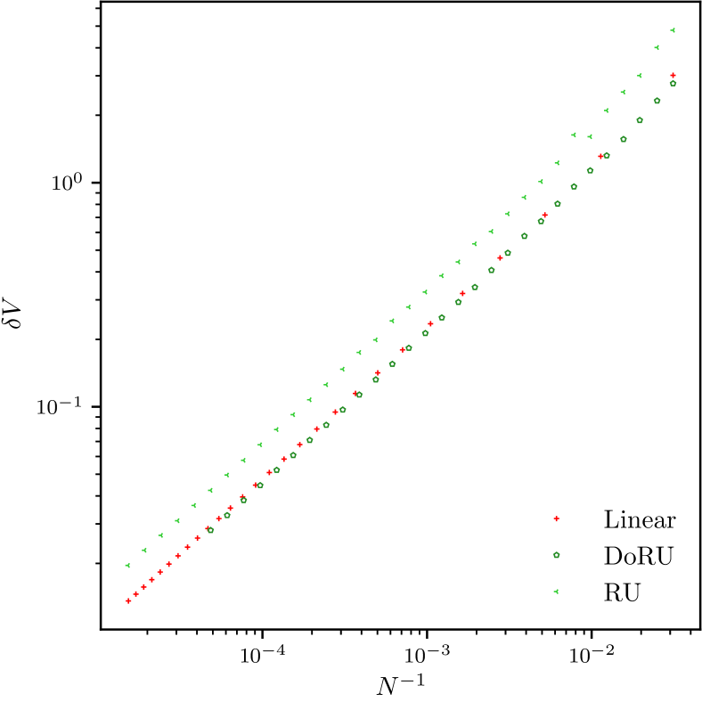
Figure 9: Like fig. 3, but comparing Linear, Distance optimised (DoRU) and Random Uniform (RU) partitionings.

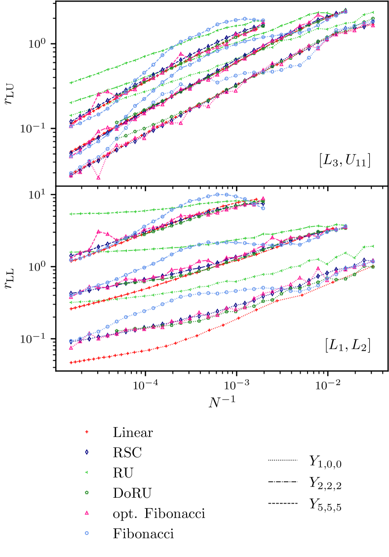
Figure 10: Showing the commutator convergence like in fig. 5, comparing RSC, Distance optimised (DoRU), Random Uniform (RU) as well as optimised and unoptimised Fibonacci partitionings.

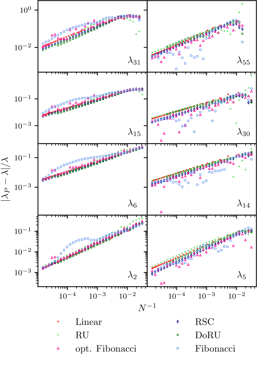
Figure 11: Convergence of the eigenvalues like in fig. 7, comparing RSC, Distance optimised (DoRU), Random Uniform (RU) as well as optimised and unoptimised Fibonacci partitionings.

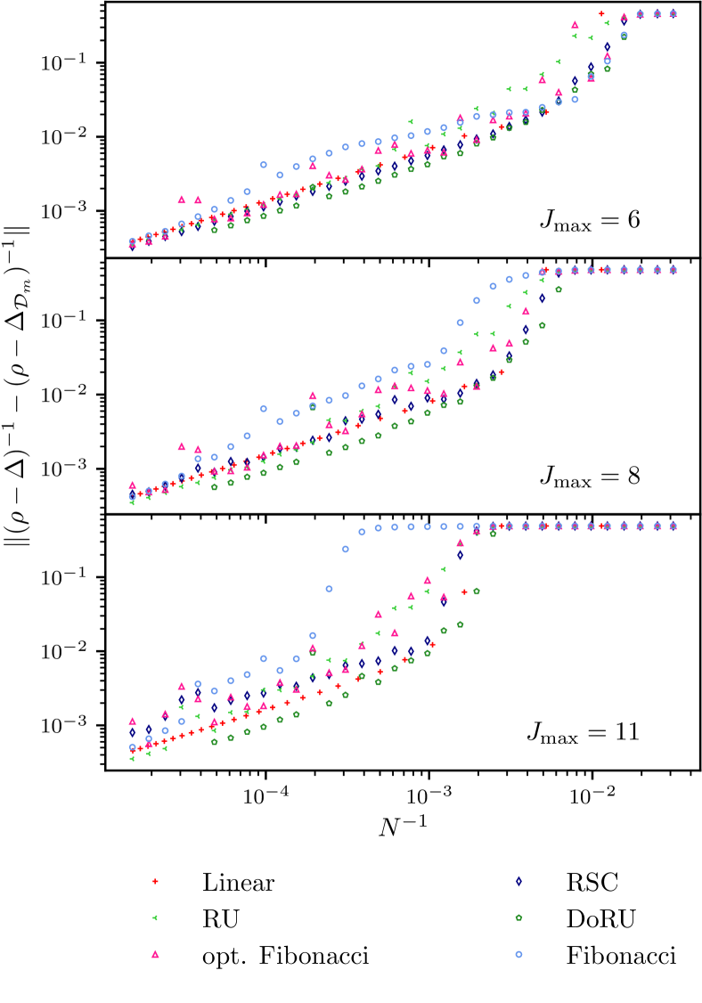
Figure 12: Operator convergence like in fig. 8, comparing RSC, Distance optimised (DoRU), Random Uniform (RU) as well as optimised and unoptimised Fibonacci partitionings.

The first thing worth noting is that the deficiencies of the unoptimised Fibonacci lattices carry over to all the discussed observables. Bumps similar to the ones observed in fig. 3 can also be found in the commutators, spectrum and operator convergence. Optimising the coefficients $a_{1}$ and $a_{2}$ again fixes this mostly and leads to a more consistent convergence behaviour. The more noisy convergence behaviour, however, remains, with occasional outliers visible.

As one might expect from the initial volume convergence results found in fig. 4, the RSC partitionings perform fairly similar to the RFCC partitionings in the other observables, too.

For the RU and DoRU partitionings the situation is a bit more intricate: in the volume, fig. 9, RU shows larger deviations at fixed $N$, which is a result of the local clustering. But the convergence rate appears to be identical to the other shown partitionings. This is also true for all the other observables with the notable exception of $r_{\mathrm{LL}}$, where RU seem to show a slower convergence, similar to the ones observed for the Genz points. The DoRU partitioning, although initially in line with the RSC points, also seems to tend towards this slower convergence rate for larger $N$. At this point it is, however, unclear whether this is inherent to the partitioning or related to the fact that the optimisation with large $N$ becomes more and more difficult. One more interesting result is that the DoRU appears to have the smallest amplitude in the gap convergence, see fig. 12.

References

- Kogut and Susskind (1975) John B. Kogut and Leonard Susskind, “Hamiltonian Formulation of Wilson’s Lattice Gauge Theories,” Phys. Rev. D 11, 395–408 (1975).
- Silvi et al. (2014) Pietro Silvi, Enrique Rico, Tommaso Calarco, and Simone Montangero, “Lattice gauge tensor networks,” New J. Phys. 16, 103015 (2014).
- Dalmonte and Montangero (2016) M. Dalmonte and S. Montangero, “Lattice gauge theory simulations in the quantum information era,” Contemp. Phys. 57, 388–412 (2016).
- Bañuls and Cichy (2020) Mari Carmen Bañuls and Krzysztof Cichy, “Review on novel methods for lattice gauge theories,” Rep. Prog. Phys. 83, 024401 (2020).
- Bañuls et al. (2020) Mari Carmen Bañuls, Rainer Blatt, Jacopo Catani, Alessio Celi, Juan Ignacio Cirac, Marcello Dalmonte, Leonardo Fallani, Karl Jansen, Maciej Lewenstein, Simone Montangero, Christine A. Muschik, Benni Reznik, Enrique Rico, Luca Tagliacozzo, Karel Van Acoleyen, Frank Verstraete, Uwe-Jens Wiese, Matthew Wingate, Jakub Zakrzewski, and Peter Zoller, “Simulating lattice gauge theories within quantum technologies,” The European Physical Journal D 74, 165 (2020).
- Bañuls et al. (2019) Mari Carmen Bañuls, Krzysztof Cichy, J. Ignacio Cirac, Karl Jansen, and Stefan Kühn, “Tensor networks and their use for lattice gauge theories,” PoS(LATTICE 2018)022 (2019), 10.22323/1.334.0022.
- Buyens et al. (2014) Boye Buyens, Jutho Haegeman, Karel Van Acoleyen, Henri Verschelde, and Frank Verstraete, “Matrix product states for gauge field theories,” Phys. Rev. Lett. 113, 091601 (2014).
- Kühn et al. (2015) Stefan Kühn, Erez Zohar, J.Ignacio Cirac, and Mari Carmen Bañuls, “Non-abelian string breaking phenomena with matrix product states,” J. High Energy Phys. 2015, 130 (2015).
- Pichler et al. (2016) T. Pichler, M. Dalmonte, E. Rico, P. Zoller, and S. Montangero, “Real-time dynamics in u(1) lattice gauge theories with tensor networks,” Phys. Rev. X 6, 011023 (2016).
- Buyens et al. (2017) Boye Buyens, Jutho Haegeman, Florian Hebenstreit, Frank Verstraete, and Karel Van Acoleyen, “Real-time simulation of the schwinger effect with matrix product states,” Phys. Rev. D 96, 114501 (2017).
- Banuls et al. (2019) Mari Carmen Banuls, Michal P. Heller, Karl Jansen, Johannes Knaute, and Viktor Svensson, “From spin chains to real-time thermal field theory using tensor networks,” Phys. Rev. Research 2, 033301 (2020) (2019), 10.1103/PhysRevResearch.2.033301.
- Rigobello et al. (2021) Marco Rigobello, Simone Notarnicola, Giuseppe Magnifico, and Simone Montangero, “Entanglement generation in 1+1d QED scattering processes,” Phys. Rev. D 104, 114501 (2021).
- Bañuls et al. (2017) Mari Carmen Bañuls, Krzysztof Cichy, J. Ignacio Cirac, Karl Jansen, and Stefan Kühn, “Density induced phase transitions in the schwinger model: A study with matrix product states,” Phys. Rev. Lett. 118, 071601 (2017).
- Silvi et al. (2017) Pietro Silvi, Enrique Rico, Marcello Dalmonte, Ferdinand Tschirsich, and Simone Montangero, “Finite-density phase diagram of a (1+1)-d non-abelian lattice gauge theory with tensor networks,” Quantum 1, 9 (2017).
- Felser et al. (2020) Timo Felser, Pietro Silvi, Mario Collura, and Simone Montangero, “Two-Dimensional Quantum-Link Lattice Quantum Electrodynamics at Finite Density,” Phys. Rev. X 10, 041040 (2020).
- Silvi et al. (2019) Pietro Silvi, Yannick Sauer, Ferdinand Tschirsich, and Simone Montangero, “Tensor network simulation of an SU(3) lattice gauge theory in 1d,” Physical Review D 100 (2019), 10.1103/physrevd.100.074512.
- Byrnes and Yamamoto (2006) Tim Byrnes and Yoshihisa Yamamoto, “Simulating lattice gauge theories on a quantum computer,” Phys. Rev. A 73, 022328 (2006).
- Jordan et al. (2012) Stephen P. Jordan, Keith S. M. Lee, and John Preskill, “Quantum algorithms for quantum field theories,” Science 336, 1130–1133 (2012).
- Mathis et al. (2020) Simon V. Mathis, Guglielmo Mazzola, and Ivano Tavernelli, “Toward scalable simulations of lattice gauge theories on quantum computers,” Phys. Rev. D 102, 094501 (2020).
- Feynman (1982) Richard P. Feynman, “Simulating physics with computers,” Int. J. Theor. Phys. 21, 467–488 (1982).
- Klco et al. (2020a) Natalie Klco, Jesse R. Stryker, and Martin J. Savage, “Su(2) non-abelian gauge field theory in one dimension on digital quantum computers,” Phys. Rev. D 101, 074512 (2020a).
- Atas et al. (2021a) Yasar Atas, Jinglei Zhang, Randy Lewis, Amin Jahanpour, Jan F. Haase, and Christine A. Muschik, “Su(2) hadrons on a quantum computer,” Nat Commun. 12, 6499 (2021a).
- Ciavarella et al. (2021a) Anthony Ciavarella, Natalie Klco, and Martin J. Savage, “Trailhead for quantum simulation of su(3) yang-mills lattice gauge theory in the local multiplet basis,” Phys. Rev. D 103, 094501 (2021a).
- Clemente et al. (2022) Giuseppe Clemente, Arianna Crippa, and Karl Jansen, “Strategies for the determination of the running coupling of (2+1)-dimensional QED with quantum computing,” Phys. Rev. D 106, 114511 (2022), arXiv:2206.12454 [hep-lat] .
- Banerjee et al. (2012) D. Banerjee, M. Dalmonte, M. Müller, E. Rico, P. Stebler, U.-J. Wiese, and P. Zoller, “Atomic quantum simulation of dynamical gauge fields coupled to fermionic matter: From string breaking to evolution after a quench,” Phys. Rev. Lett. 109, 175302 (2012).
- Tagliacozzo et al. (2013a) L. Tagliacozzo, A. Celi, A. Zamora, and M. Lewenstein, “Optical abelian lattice gauge theories,” Ann. Phys. 330, 160 – 191 (2013a).
- Tagliacozzo et al. (2013b) L. Tagliacozzo, A. Celi, P. Orland, M. W. Mitchell, and M. Lewenstein, “Simulation of non-abelian gauge theories with optical lattices,” Nat. Commun. 4, 2615 (2013b).
- Büchler et al. (2005) H. P. Büchler, M. Hermele, S. D. Huber, Matthew P. A. Fisher, and P. Zoller, “Atomic quantum simulator for lattice gauge theories and ring exchange models,” Phys. Rev. Lett. 95, 040402 (2005).
- Zohar and Reznik (2011) Erez Zohar and Benni Reznik, “Confinement and lattice quantum-electrodynamic electric flux tubes simulated with ultracold atoms,” Phys. Rev. Lett. 107, 275301 (2011).
- Zohar et al. (2012) Erez Zohar, J. Ignacio Cirac, and Benni Reznik, “Simulating compact quantum electrodynamics with ultracold atoms: Probing confinement and nonperturbative effects,” Phys. Rev. Lett. 109, 125302 (2012).
- Hauke et al. (2013) P. Hauke, D. Marcos, M. Dalmonte, and P. Zoller, “Quantum simulation of a lattice schwinger model in a chain of trapped ions,” Phys. Rev. X 3, 041018 (2013).
- Zohar et al. (2013a) Erez Zohar, J. Ignacio Cirac, and Benni Reznik, “Cold-atom quantum simulator for su(2) yang-mills lattice gauge theory,” Phys. Rev. Lett. 110, 125304 (2013a).
- Zohar et al. (2013b) Erez Zohar, J. Ignacio Cirac, and Benni Reznik, “Simulating ()-dimensional lattice qed with dynamical matter using ultracold atoms,” Phys. Rev. Lett. 110, 055302 (2013b).
- Banerjee et al. (2013) D. Banerjee, M. Bögli, M. Dalmonte, E. Rico, P. Stebler, U.-J. Wiese, and P. Zoller, “Atomic quantum simulation of u(n) and su(n) non-abelian lattice gauge theories,” Phys. Rev. Lett. 110, 125303 (2013).
- Zohar et al. (2016) Erez Zohar, J Ignacio Cirac, and Benni Reznik, “Quantum simulations of lattice gauge theories using ultracold atoms in optical lattices,” Rep. Prog. Phys. 79, 014401 (2016).
- Laflamme et al. (2016) C. Laflamme, W. Evans, M. Dalmonte, U. Gerber, H. Mejía-Díaz, W. Bietenholz, U.-J. Wiese, and P. Zoller, “Cp(n-1) quantum field theories with alkaline-earth atoms in optical lattices,” Ann. Phys. 370, 117 – 127 (2016).
- González-Cuadra et al. (2017) Daniel González-Cuadra, Erez Zohar, and J. Ignacio Cirac, “Quantum simulation of the abelian-higgs lattice gauge theory with ultracold atoms,” New J. Phys. 19, 063038 (2017).
- Rico et al. (2018) E. Rico, M. Dalmonte, P. Zoller, D. Banerjee, M. Bögli, P. Stebler, and U.-J. Wiese, “So(3) “nuclear physics” with ultracold gases,” Annals of Physics 393, 466–483 (2018).
- Zache et al. (2018) T V Zache, F Hebenstreit, F Jendrzejewski, M K Oberthaler, J Berges, and P Hauke, “Quantum simulation of lattice gauge theories using wilson fermions,” Quantum Science and Technology 3, 034010 (2018).
- Klco et al. (2018a) N. Klco, E. F. Dumitrescu, A. J. McCaskey, T. D. Morris, R. C. Pooser, M. Sanz, E. Solano, P. Lougovski, and M. J. Savage, “Quantum-classical computation of schwinger model dynamics using quantum computers,” Phys. Rev. A 98 (2018a), 10.1103/physreva.98.032331.
- Mazzola et al. (2021) Giulia Mazzola, Simon V. Mathis, Guglielmo Mazzola, and Ivano Tavernelli, “Gauge-invariant quantum circuits for (1) and yang-mills lattice gauge theories,” Phys. Rev. Research 3, 043209 (2021).
- Martinez et al. (2016) E. A. Martinez, C. A. Muschik, P. Schindler, D. Nigg, A. Erhard, M. Heyl, P. Hauke, M. Dalmonte, T. Monz, P. Zoller, and R. Blatt, “Real-time dynamics of lattice gauge theories with a few-qubit quantum computer,” Nature 534, 516 (2016).
- Kokail et al. (2019) Christian Kokail, Christine Maier, Rick van Bijnen, Tiff Brydges, Manoj K. Joshi, Petar Jurcevic, Christine A. Muschik, Pietro Silvi, Rainer Blatt, Christian F. Roos, and Peter Zoller, “Self-verifying variational quantum simulation of the lattice schwinger model,” Nature 569, 355 (2019).
- Funcke et al. (2023) Lena Funcke, Tobias Hartung, Karl Jansen, and Stefan Kühn, “Review on Quantum Computing for Lattice Field Theory,” in 39th International Symposium on Lattice Field Theory (2023) arXiv:2302.00467 [hep-lat] .
- Davoudi et al. (2021) Zohreh Davoudi, Indrakshi Raychowdhury, and Andrew Shaw, “Search for efficient formulations for Hamiltonian simulation of non-Abelian lattice gauge theories,” Phys. Rev. D 104, 074505 (2021), arXiv:2009.11802 [hep-lat] .
- Klco et al. (2018b) N. Klco, E. F. Dumitrescu, A. J. McCaskey, T. D. Morris, R. C. Pooser, M. Sanz, E. Solano, P. Lougovski, and M. J. Savage, “Quantum-classical computation of Schwinger model dynamics using quantum computers,” Phys. Rev. A 98, 032331 (2018b), arXiv:1803.03326 [quant-ph] .
- Lewis and Woloshyn (2019) Randy Lewis and R. M. Woloshyn, “A qubit model for U(1) lattice gauge theory,” (2019) arXiv:1905.09789 [hep-lat] .
- Paulson et al. (2021) Danny Paulson et al., “Towards simulating 2D effects in lattice gauge theories on a quantum computer,” PRX Quantum 2, 030334 (2021), arXiv:2008.09252 [quant-ph] .
- Haase et al. (2021) Jan F. Haase, Luca Dellantonio, Alessio Celi, Danny Paulson, Angus Kan, Karl Jansen, and Christine A. Muschik, “A resource efficient approach for quantum and classical simulations of gauge theories in particle physics,” Quantum 5, 393 (2021), arXiv:2006.14160 [quant-ph] .
- Nguyen et al. (2022) Nhung H. Nguyen, Minh C. Tran, Yingyue Zhu, Alaina M. Green, C. Huerta Alderete, Zohreh Davoudi, and Norbert M. Linke, “Digital Quantum Simulation of the Schwinger Model and Symmetry Protection with Trapped Ions,” PRX Quantum 3, 020324 (2022), arXiv:2112.14262 [quant-ph] .
- Klco et al. (2020b) Natalie Klco, Jesse R. Stryker, and Martin J. Savage, “SU(2) non-Abelian gauge field theory in one dimension on digital quantum computers,” Phys. Rev. D 101, 074512 (2020b), arXiv:1908.06935 [quant-ph] .
- Atas et al. (2021b) Yasar Y. Atas, Jinglei Zhang, Randy Lewis, Amin Jahanpour, Jan F. Haase, and Christine A. Muschik, “SU(2) hadrons on a quantum computer via a variational approach,” Nature Commun. 12, 6499 (2021b), arXiv:2102.08920 [quant-ph] .
- A Rahman et al. (2021) Sarmed A Rahman, Randy Lewis, Emanuele Mendicelli, and Sarah Powell, “SU(2) lattice gauge theory on a quantum annealer,” Phys. Rev. D 104, 034501 (2021), arXiv:2103.08661 [hep-lat] .
- Ciavarella et al. (2021b) Anthony Ciavarella, Natalie Klco, and Martin J. Savage, “Trailhead for quantum simulation of SU(3) Yang-Mills lattice gauge theory in the local multiplet basis,” Phys. Rev. D 103, 094501 (2021b), arXiv:2101.10227 [quant-ph] .
- A Rahman et al. (2022a) Sarmed A Rahman, Randy Lewis, Emanuele Mendicelli, and Sarah Powell, “Self-mitigating Trotter circuits for SU(2) lattice gauge theory on a quantum computer,” Phys. Rev. D 106, 074502 (2022a), arXiv:2205.09247 [hep-lat] .
- Atas et al. (2022) Yasar Y. Atas, Jan F. Haase, Jinglei Zhang, Victor Wei, Sieglinde M. L. Pfaendler, Randy Lewis, and Christine A. Muschik, “Real-time evolution of SU(3) hadrons on a quantum computer,” (2022), arXiv:2207.03473 [quant-ph] .
- Catumba et al. (2022) Guilherme Catumba, Atsuki Hiraguchi, George W. S. Hou, Karl Jansen, Ying-Jer Kao, C. J. David Lin, Alberto Ramos, and Mugdha Sarkar, “Study of SU(2) gauge theories with multiple Higgs fields in different representations,” in 39th International Symposium on Lattice Field Theory (2022) arXiv:2210.09855 [hep-lat] .
- A Rahman et al. (2022b) Sarmed A Rahman, Randy Lewis, Emanuele Mendicelli, and Sarah Powell, “Real time evolution and a traveling excitation in SU(2) pure gauge theory on a quantum computer,” in 39th International Symposium on Lattice Field Theory (2022) arXiv:2210.11606 [hep-lat] .
- Gustafson et al. (2022) Erik J. Gustafson, Henry Lamm, Felicity Lovelace, and Damian Musk, “Primitive quantum gates for an SU(2) discrete subgroup: Binary tetrahedral,” Phys. Rev. D 106, 114501 (2022), arXiv:2208.12309 [quant-ph] .
- Farrell et al. (2023a) Roland C. Farrell, Ivan A. Chernyshev, Sarah J. M. Powell, Nikita A. Zemlevskiy, Marc Illa, and Martin J. Savage, “Preparations for quantum simulations of quantum chromodynamics in 1+1 dimensions. I. Axial gauge,” Phys. Rev. D 107, 054512 (2023a), arXiv:2207.01731 [quant-ph] .
- Farrell et al. (2023b) Roland C. Farrell, Ivan A. Chernyshev, Sarah J. M. Powell, Nikita A. Zemlevskiy, Marc Illa, and Martin J. Savage, “Preparations for quantum simulations of quantum chromodynamics in 1+1 dimensions. II. Single-baryon -decay in real time,” Phys. Rev. D 107, 054513 (2023b), arXiv:2209.10781 [quant-ph] .
- Alam et al. (2022) M. Sohaib Alam, Stuart Hadfield, Henry Lamm, and Andy C. Y. Li (SQMS), “Primitive quantum gates for dihedral gauge theories,” Phys. Rev. D 105, 114501 (2022), arXiv:2108.13305 [quant-ph] .
- Carena et al. (2022) Marcela Carena, Henry Lamm, Ying-Ying Li, and Wanqiang Liu, “Improved Hamiltonians for Quantum Simulations of Gauge Theories,” Phys. Rev. Lett. 129, 051601 (2022), arXiv:2203.02823 [hep-lat] .
- Gustafson and Lamm (2023) Erik J. Gustafson and Henry Lamm, “Robustness of Gauge Digitization to Quantum Noise,” (2023), arXiv:2301.10207 [hep-lat] .
- Chandrasekharan and Wiese (1997) S. Chandrasekharan and U. J. Wiese, “Quantum link models: A Discrete approach to gauge theories,” Nucl. Phys. B 492, 455–474 (1997), arXiv:hep-lat/9609042 .
- Brower et al. (1999) R. Brower, S. Chandrasekharan, and U. J. Wiese, “QCD as a quantum link model,” Phys. Rev. D 60, 094502 (1999), arXiv:hep-th/9704106 .
- Wiese (2021) Uwe-Jens Wiese, “From quantum link models to D-theory: a resource efficient framework for the quantum simulation and computation of gauge theories,” Phil. Trans. A. Math. Phys. Eng. Sci. 380, 20210068 (2021), arXiv:2107.09335 [hep-lat] .
- Davoudi et al. (2022) Zohreh Davoudi, Alexander F. Shaw, and Jesse R. Stryker, “General quantum algorithms for Hamiltonian simulation with applications to a non-Abelian lattice gauge theory,” (2022), arXiv:2212.14030 [hep-lat] .
- Hartung et al. (2022) Tobias Hartung, Timo Jakobs, Karl Jansen, Johann Ostmeyer, and Carsten Urbach, “Digitising SU(2) gauge fields and the freezing transition,” Eur. Phys. J. C 82, 237 (2022), arXiv:2201.09625 [hep-lat] .
- Jakobs et al. (2023) Timo Jakobs, Tobias Hartung, Karl Jansen, Johann Ostmeyer, and Carsten Urbach, “Digitizing SU(2) gauge fields and what to look out for when doing so,” PoS LATTICE2022, 015 (2023), arXiv:2212.09496 [hep-lat] .
- Ji et al. (2020) Yao Ji, Henry Lamm, and Shuchen Zhu (NuQS), “Gluon Field Digitization via Group Space Decimation for Quantum Computers,” Phys. Rev. D 102, 114513 (2020), arXiv:2005.14221 [hep-lat] .
- Alexandru et al. (2019) Andrei Alexandru, Paulo F. Bedaque, Siddhartha Harmalkar, Henry Lamm, Scott Lawrence, and Neill C. Warrington (NuQS), “Gluon Field Digitization for Quantum Computers,” Phys. Rev. D 100, 114501 (2019), arXiv:1906.11213 [hep-lat] .
- Alexandru et al. (2022) Andrei Alexandru, Paulo F. Bedaque, Ruairí Brett, and Henry Lamm, “Spectrum of digitized QCD: Glueballs in a S(1080) gauge theory,” Phys. Rev. D 105, 114508 (2022), arXiv:2112.08482 [hep-lat] .
- Ji et al. (2022) Yao Ji, Henry Lamm, and Shuchen Zhu, “Gluon Digitization via Character Expansion for Quantum Computers,” (2022), arXiv:2203.02330 [hep-lat] .
- Garofalo et al. (2022) Marco Garofalo, Tobias Hartung, Karl Jansen, Johann Ostmeyer, Simone Romiti, and Carsten Urbach, “Defining Canonical Momenta for Discretised SU(2) Gauge Fields,” in 39th International Symposium on Lattice Field Theory (2022) arXiv:2210.15547 [hep-lat] .
- Crane et al. (2013) Keenan Crane, Fernando de Goes, Mathieu Desbrun, and Peter Schröder, “Digital geometry processing with discrete exterior calculus,” ACM SIGGRAPH 2013 courses, SIGGRAPH ’13 (2013).
- Correa et al. (2011) Carlos D. Correa, Robert Hero, and Kwan-Liu Ma, “A comparison of gradient estimation methods for volume rendering on unstructured meshes,” IEEE Transactions on Visualization and Computer Graphics 17, 305–319 (2011).
- Crane (2019) Keenan Crane, “The n-dimensional cotangent formula,” (2019).
- Delaunay (1934) B. N. Delaunay, “Sur la sphère vide,” Bulletin of Academy of Sciences of the USSR 7, 793–800 (1934).
- Hahn (2001) Theo Hahn, ed., International tables for crystallography: Space group symmetry v. A, 5th ed. (Kluwer Academic, Tucson, AZ, 2001).
- Hales (2006) Thomas C. Hales, “Historical overview of the kepler conjecture,” Discrete & Computational Geometry 36, 5–20 (2006).
- Hartung (2015) T. Hartung, -function of Fourier Integral Operator, Ph.D. thesis, King’s College London (2015).
- Erdélyi et al. (1953) Arthur Erdélyi, W Magnus, F Oberhettinger, and FG Tricomi, “Bateman manuscript project,” Higher transcendental functions 2, 133 (1953).
- Kato (1966) Tosio Kato, Perturbation Theory for Linear Operators (Springer, 1966).