Graphene valley polarization as a function of carrier-envelope phase in few-cycle laser pulses and its footprints in harmonic signals

Abstract

We consider coherent dynamics of graphene charged carriers exposed to an intense few-cycle linearly polarized laser pulse. The results, obtained by solving the generalized semiconductor Bloch equations numerically in the Hartree-Fock approximation, taking into account many-body Coulomb interaction, demonstrate strong dependence of the valley polarization on the carrier-envelope phase (CEP), which is interpolated by the simple sinusoidal law. Then we consider harmonic generation in multi-cycle laser field by graphene preliminary exposed to an intense few-cycle laser pulse. We show that the second harmonic’s intensity is a robust observable quantity that provides a gauge of CEP for pulse durations up to two optical cycles, corresponding to 40 $\mathrm{fs}$ at the wavelength of 6.2 $\mathrm{\mu m}$.

I Introduction

In many semiconductor and semimetal materials, conduction band electrons occupy states near several discrete energy minima which have been termed valleys. In general, electrons in these discrete valley-states have different properties, which results in a valley-dependent electromagnetic (EM) response in these materials. Hence, in addition to electron spin, we have an additional degree of freedom – valley isospin or valley polarization. In analogy with the spintronics for spin-based technology, it has been proposed the valleytronics Rycerz et al. (2007); Vitale et al. (2018); Schaibley et al. (2016) that has attracted a considerable attention because of its possible application in quantum information science. Experimentally the valley-polarization of electrons was achieved in several materials. In AlAs, valley polarization was induced by a symmetry-breaking strain Gunawan et al. (2006), in bismuth - by using a rotating magnetic field Zhu et al. (2012), in diamond -by electrostatic control of valley currents Isberg et al. (2013); Suntornwipat et al. (2020), in MoS₂ -by means of circularly polarized light due to valley-contrasting Berry curvature Cao et al. (2012); Mak et al. (2012); Zeng et al. (2012); Li et al. (2020).

The valley polarization is sensitive to thermal lattice vibrations and for valleytronics applications, it is necessary materials where the valley polarization relaxation time is remarkably long. From this point of view graphene Castro Neto et al. (2009), where the intervalley scattering is suppressed Morpurgo and Guinea (2006); Morozov et al. (2006); McCann et al. (2006), is of interest. For graphene, there are two inequivalent Dirac points in the Brillouin zone, related by time-reversal and inversion symmetry Castro Neto et al. (2009). Hence, the valley-contrasting Berry curvature is zero that makes it difficult to use graphene in valleytronics, especially if one wants to use intense light pulses for ultrafast manipulation of valley polarization. A number of proposals on how to break time-reversal or inversion symmetry in graphene based materials for generation of the valley polarization has been put forward. Valley polarization in graphene sheet can be achieved with zigzag edges Rycerz et al. (2007), at a line defect Gunlycke and White (2011), for strained graphene with massive Dirac fermions Grujić et al. (2014); Faria et al. (2020) and with broken inversion symmetry Xiao et al. (2007); Yankowitz et al. (2012), through a boundary between the monolayer and bilayer graphene Nakanishi et al. (2010); Pratley and Zülicke (2014). Valley polarization in graphene can also be achieved at the breaking time-reversal symmetry with AC mechanical vibrations Jiang et al. (2013). Regarding the light-wave manipulation of valleys, it was shown that valley currents can be induced by asymmetric monocycle EM pulses Moskalenko and Berakdar (2009) or by specifically polarized light Golub et al. (2011). Recently, for gapped graphene like systems, such as hexagonal boron nitride and molybdenum disulfide several schemes for light-wave manipulation of valleys have been proposed which do not rely on valley-contrasting Berry curvature. One with two-color counter-rotating circularly polarized laser pulses Jiménez-Galán et al. (2020) and the other by exploiting the carrier-envelope phase (CEP) of ultrashort linearly polarized pulse Jiménez-Galán et al. (2021), or circularly polarized pulse Oliaei Motlagh et al. (2019). Successful attempts have been made to apply these schemes to intrinsic graphene Mrudul et al. (2021); Mrudul and Dixit (2021); Kelardeh et al. (2022), where for the linear polarization of the driving wave the main emphases have been made to subcycle laser pulses Kelardeh et al. (2022).

The problem of coherent interaction of graphene with an intense few-cycle linearly polarized laser pulse can be applied to solve two important issues regarding the valleytronics and light-wave electronics Goulielmakis et al. (2007). For valleytronics, it can be an efficient method to reach valley-polarization which depends on the carrier-envelope phase, and vice versa, to measure CEP via the valley-polarization which is important for short pulse manipulation. As is well known, the second harmonic is sensitive to valley-polarization Golub and Tarasenko (2014); Wehling et al. (2015); Ho et al. (2020), which opens a door for solving the mentioned issues. In the present paper, we address these problems considering the coherent dynamics of graphene charged carriers exposed to an intense few-cycle linearly polarized laser pulse. We numerically solve the generalized semiconductor Bloch equations in the Hartree-Fock approximation Malic et al. (2011); Avetissian and Mkrtchian (2018); Avetissian et al. (2022) taking into account the many-body Coulomb interaction and demonstrate the strong dependence of the valley polarization on the CEP, which is interpolated by the simple harmonic law. Then we consider the harmonic generation in a multi-cycle laser pulse-field by graphene preliminary exposed to an intense few-cycle laser pulse and consider the ways to gauge the CEP.

The paper is organized as follows. In Sec. II, the model and the basic equations are formulated. In Sec. III, we present the main results. Finally, conclusions are given in Sec. IV.

II The model and theoretical methods

We begin by describing the model and theoretical approach. Two dimensional hexagonal nanostructure is assumed to interact with a few cycle mid-infrared laser pulse that excites coherent electron dynamics which is subsequently probed by an intense near-infrared or visible light pulse generating high harmonics. It is assumed that the polarization planes of both laser fields coincide with the nanostructure plane ($XY$). For numerical convenience and to avoid residual momentum transfer, the electric field $\mathbf{E}\left(t\right)$ is calculated from the expression of the vector potential given by

$$\mathbf{A}\left(t\right)=f_{0}\left(t\right)A_{0}\hat{\mathbf{e}}_{0}\sin\left(\omega_{0}t+\phi_{\mathrm{CEP}}\right)$$

$$+f_{1}\left(t\right)A_{1}\hat{\mathbf{e}}_{1}\sin\left(\omega_{1}t+\phi_{\mathrm{CEP}1}\right),$$ (1)

where $A_{0}$ and $A_{1}$ are the amplitudes of the vector potentials which are connected to the amplitudes of the applied electric fields $E_{0}=\omega_{0}A_{0}$ and $E_{1}=\omega_{1}A_{1}$ of the laser pulses, $\omega_{0}$ and $\omega_{1}$ are the fundamental frequencies, $\hat{\mathbf{e}}_{0}$ and $\hat{\mathbf{e}}_{1}$ are the unit polarization vectors, $\phi_{\mathrm{CEP}}$ and $\phi_{\mathrm{CEP}1}$ are carrier-envelope phases. The envelopes of the two waves are described by the sin-squared functions

$$f_{0,1}(t+t_{0,1})=\left\{\begin{array}[]{cc}\sin^{2}\left(\pi t/\tau_{0,1}\right),&0\leq t\leq\tau_{0,1},\\ 0,&t<0,t>\tau_{0,1},\end{array}\right.$$ (2)

where $\tau_{0}$ and $\tau_{1}$ characterize the pulses’ duration, and $t_{1}$ and $t_{2}$ define the starts of the pulses. For a probe wave we will assume $\tau_{1}>>2\pi/\omega_{1}$. In this case the detailed behavior of the electric field dependence on the carrier-envelope phase is not important. Hence we take $\phi_{\mathrm{CEP}1}=0$. For a few-cycle pump pulse the exact position of nodes and peaks of the electric field is of great importance, since it determines the momentum distribution of the excited electrons, which in turn defines harmonics spectrum during the interaction with the probe pulse. For a pump wave-pulse the envelope $f_{0}(t)$ is chosen such that the maximal electric field strength is reached at $t=0$ and $\phi_{\mathrm{CEP}}=0$.

Monolayer graphene interaction with the EM field is described using generalized semiconductor Bloch equations in the Hartree-Fock approximation. Technical details can be found in Refs. Malic et al. (2011); Avetissian and Mkrtchian (2018); Avetissian et al. (2022), while for self-consistency the main equations are outlined below. Thus, the Bloch equations within the Houston basis read

$$\partial_{t}\mathcal{N}(\mathbf{k}_{0},t)=-2\mathrm{Im}\left\{\left[\mathbf{E}\left(t\right)\mathbf{D}_{\mathrm{tr}}\left(\mathbf{k}_{0}+\mathbf{A}\right)\right.\right.$$

$$\left.\left.+\Omega_{c}\left(\mathbf{k}_{0}+\mathbf{A},t;\mathcal{P},\mathcal{N}\right)\right]\mathcal{P}^{\ast}(\mathbf{k}_{0},t)\right\},$$ (3)

$$\partial_{t}\mathcal{P}(\mathbf{k}_{0},t)=-i\left[\mathcal{E}_{eh}\left(\mathbf{k}_{0}+\mathbf{A}\right)-i\Gamma\right]\mathcal{P}(\mathbf{k}_{0},t)$$

$$+i\left[\mathbf{E}\left(t\right)\mathbf{D}_{\mathrm{tr}}\left(\mathbf{k}_{0}+\mathbf{A}\right)+\Omega_{c}\left(\mathbf{k}_{0}+\mathbf{A},t;\mathcal{P},\mathcal{N}\right)\right]$$

$$\times\left[1-2\mathcal{N}(\mathbf{k}_{0},t)\right],$$ (4)

where $\mathcal{P}(\mathbf{k},t)=\mathcal{P}^{\prime}(\mathbf{k},t)+i\mathcal{P}^{\prime\prime}(\mathbf{k},t)$ is the interband polarization and $\mathcal{N}\left(\mathbf{k},t\right)$ is the electron distribution function for the conduction band. The electron-hole energy

$$\mathcal{E}_{eh}\left(\mathbf{k}\right)=2\mathcal{E}\left(\mathbf{k}\right)-\Xi_{c}(\mathbf{k},t;\mathcal{P},\mathcal{N})$$ (5)

is defined via the band energy

$$\mathcal{E}\left(\mathbf{k}\right)=\gamma_{0}\left|f\left(\mathbf{k}\right)\right|,$$ (6)

and many-body Coulomb interaction energy

$$\Xi_{c}(\mathbf{k},t;\mathcal{P},\mathcal{N})=\frac{2}{\left(2\pi\right)^{2}}\int_{BZ}d\mathbf{k}^{\prime}V_{2D}\left(\mathbf{k-k}^{\prime}\right)$$

$$\times\left\{f_{c}\left(\mathbf{k,k}^{\prime}\right)\mathcal{N}\left(\mathbf{k}^{\prime}\right)+f_{s}\left(\mathbf{k,k}^{\prime}\right)\mathcal{P}^{\prime\prime}\left(\mathbf{k}^{\prime},t\right)\right\}.$$ (7)

In Eqs. (6) $\gamma_{0}$ is the transfer energy of the nearest-neighbor hopping and the structure function is

$$f\left(\mathbf{k}\right)=e^{i\frac{ak_{y}}{\sqrt{3}}}+2e^{-i\frac{ak_{y}}{2\sqrt{3}}}\cos\left(\frac{ak_{x}}{2}\right),$$ (8)

where $a$ is the lattice spacing. In Eq. (7)

$$f_{c}\left(\mathbf{k,k}^{\prime}\right) = \cos\left[\mathrm{arg}f\left(\mathbf{k}^{\prime}\right)-\mathrm{arg}f\left(\mathbf{k}\right)\right],$$

$$f_{s}\left(\mathbf{k,k}^{\prime}\right) = \sin\left[\mathrm{arg}f\left(\mathbf{k}^{\prime}\right)-\mathrm{arg}f\left(\mathbf{k}\right)\right].$$

The electron-electron interaction potential is modelled by screened Coulomb potential Malic et al. (2011):

$$V_{2D}\left(\mathbf{q}\right)=\frac{2\pi}{\epsilon\epsilon_{\mathbf{q}}\left|\mathbf{q}\right|},$$ (9)

which accounts for the substrate-induced screening in the 2D nanostructure ($\epsilon$) and the screening stemming from valence electrons ($\epsilon_{\mathbf{q}}$). We take $\epsilon\simeq 4$ which is close to the value of a graphene layer sandwiched by a SiO₂. The screening induced by nanostructure valence electrons is calculated within the Lindhard approximation of the dielectric function $\epsilon_{\mathbf{q}}$. In general, one should consider the problem of dynamic screening. However, the used here ansatz is justified since the large $q$ behavior of graphene dielectric screening does not depend on the electron density Hwang and Das Sarma (2007) and we consider ultrashort time scales. In Eq. (4) $\Gamma$ is the damping rate. In Eqs. (3) and (4) the interband transitions are defined via the transition dipole moment

$$\mathbf{D}_{\mathrm{tr}}\left(\mathbf{k}\right)=-\frac{a}{2\left|f\left(\mathbf{k}\right)\right|^{2}}\sin\left(\frac{\sqrt{3}}{2}ak_{y}\right)\sin\left(\frac{ak_{x}}{2}\right)\widehat{\mathbf{x}}$$

$$+\frac{a}{2\sqrt{3}\left|f\left(\mathbf{k}\right)\right|^{2}}\left(\cos\left(ak_{x}\right)-\cos\left(\frac{\sqrt{3}}{2}ak_{y}\right)\cos\left(\frac{ak_{x}}{2}\right)\right)\widehat{\mathbf{y}},$$ (10)

and the light-matter coupling via the internal dipole field of all generated electron-hole excitations:

$$\Omega_{c}\left(\mathbf{k},t;\mathcal{P},\mathcal{N}\right)=\frac{1}{\left(2\pi\right)^{2}}\int_{BZ}d\mathbf{k}^{\prime}V_{2D}\left(\mathbf{k-k}^{\prime}\right)$$

$$\times\left\{\mathcal{P}^{\prime}\left(\mathbf{k}^{\prime},t\right)+if_{c}\left(\mathbf{k,k}^{\prime}\right)\mathcal{P}^{\prime\prime}\left(\mathbf{k}^{\prime}\right)-if_{s}\left(\mathbf{k,k}^{\prime}\right)\mathcal{N}\left(\mathbf{k}^{\prime},t\right)\right\}.$$ (11)

For compactness of equations atomic units are used throughout the paper unless otherwise indicated. The initial conditions $\mathcal{P}(\mathbf{k},0)=0$ and $\mathcal{N}(\mathbf{k},0)=0$ are assumed, neglecting thermal occupations. We will solve these equations numerically. It is more convenient to make integration of these equations in the reduced BZ which contains equivalent $\mathbf{k}$-points of the first BZ, cf. Fig. 1.

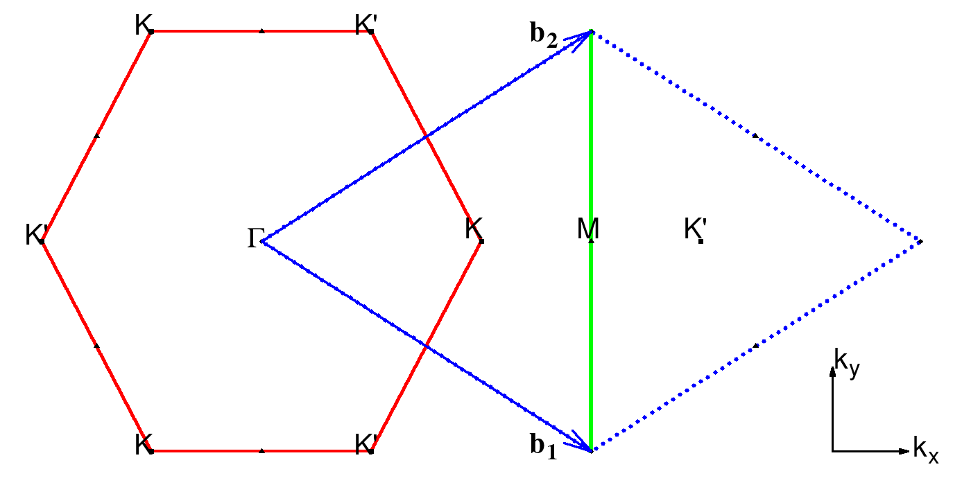
Figure 1: The hexagonal first BZ of the reciprocal lattice (red solid line). The rhombus (blue dashed lines) formed by the reciprocal lattice vectors is a reduction of the second BZ and contains the same vectors of the first BZ. The green (solid) line, that goes through M point, divides the rhombus into the left and right triangles, which contain two valleys described by the $D_{3h}$ group.

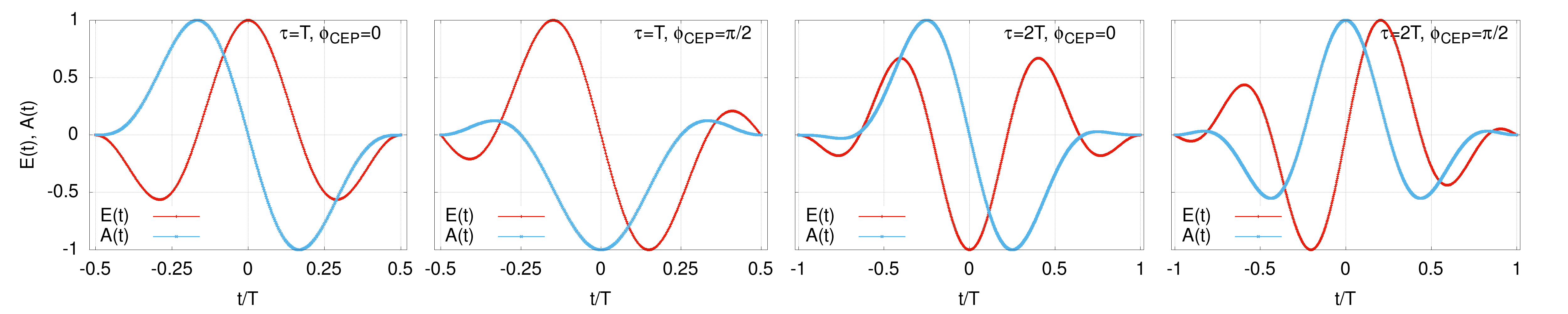
Figure 2: The electric field and vector potental normalized to maximal values versus time for one and two cycle pulses for a cosine pulse and for a sine pulse.

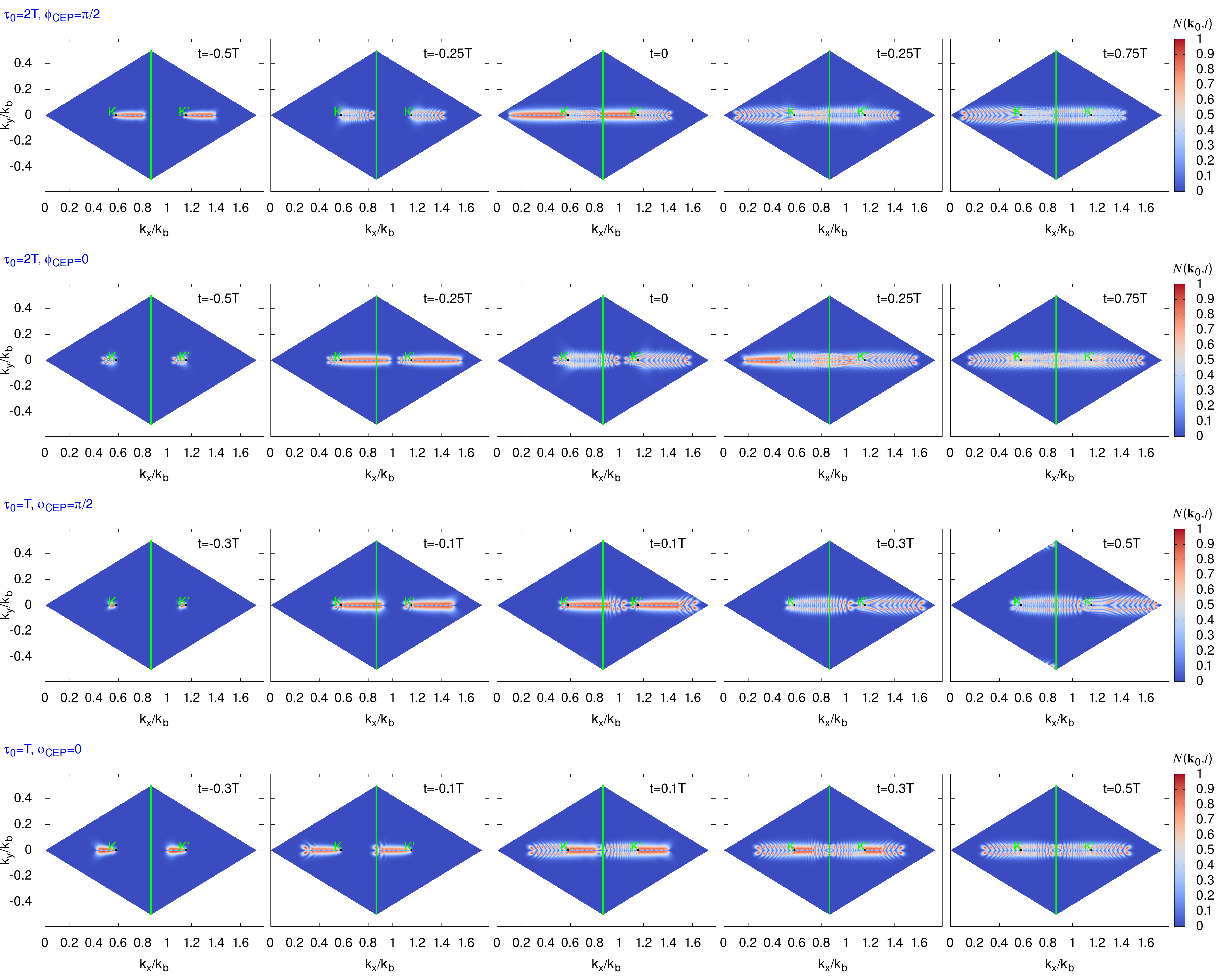
Figure 3: Particle distribution function $\mathcal{N}\left(\mathbf{k},t\right)$ (in arbitrary units) at various time instances during the interaction with the two (upper two rows) and single (3rd and 4th rows) cycle laser pulse for graphene, as a function of scaled dimensionless momentum components ($k_{x}/k_{b}$, $k_{y}/k_{b}$). The fundamental frequency is $\omega_{0}=0.2\ \mathrm{eV}/\hbar$ and the wave-particle interaction parameter is taken to be $\chi_{0}=3.5$ (intensity $1\ \mathrm{TW/cm}^{2}$).

To quantify valley polarization we introduce valley-asymmetry parameter:

$$\eta=2\frac{N_{+}-N_{-}}{N_{+}+N_{-}},$$ (12)

where $N_{-}$ and $N_{+}$ are electron populations around respective valleys and are obtained by integrating over left ($BZ_{L}$) and right triangles ($BZ_{R}$) in Fig.1:

$$N_{-}(t)=\frac{1}{\left(2\pi\right)^{2}}\int_{BZ_{L}}d\mathbf{k}\mathcal{N}\left(\mathbf{k},t\right),$$ (13)

$$N_{+}(t)=\frac{1}{\left(2\pi\right)^{2}}\int_{BZ_{R}}d\mathbf{k}\mathcal{N}\left(\mathbf{k},t\right).$$ (14)

It is clear that the denominator in Eq. (12) is the total electron population in the conduction band $N(t)$:

$$N(t)=N_{-}(t)+N_{+}(t)=\frac{1}{\left(2\pi\right)^{2}}\int_{BZ}d\mathbf{k}\mathcal{N}\left(\mathbf{k},t\right).$$ (15)

III Results

Having outlined the set-up, we first consider coherent dynamics of graphene charged carriers exposed to an intense few-cycle linearly polarized laser pulse. Our results are obtained by solving the corresponding generalized semiconductor Bloch equations (3) and (4) analytically in the free carrier approximation and numerically in the Hartree-Fock approximation taking into account many-body Coulomb interaction.

III.1 Valley polarization dependence on CEP in graphene

As is evident from Eqs. (3) and (4) the excitation pattern of BZ is defined by the vector potential of the pump pulse and to have overall valley polarization one should break the symmetry of free standing graphene. Although the crystal lattice of graphene is centrosymmetric, the valleys $K$ and $K^{\prime}$ are described by the wave vector group $D_{\mathrm{3h}}$ lacking the space inversion. These valleys are in the left and right triangles of the rhombus in Fig. 1 and are connected with each other by the space inversion $I$. Thus, the overall symmetry of free standing graphene $D_{6h}=D_{3h}\times I$ is centrosymmetric.

In Fig. 2 we plot the electric field $E\left(t\right)$ and vector potential $A\left(t\right)$ of one and two cycle pulses for a cosine pulse $\phi_{\mathrm{CEP}}=0$ and for the sine pulse $\phi_{\mathrm{CEP}}=\pi/2$. As is seen from Fig. 2, under time reversal $t\rightarrow-t$ the electric field of a cosine pulse remains invariant, while the field of a sine pulse changes sign. For the vector potential $A\left(t\right)$ that defines the excitation pattern of BZ the situation is opposite. The sine pulse has a preferred orientation of the vector potential –the orientation of the maximal field peak. The violation of symmetry has a striking manifestation in the valley polarization. To have maximal valley polarization the amplitude of the vector potential should be along $\Gamma-K$ direction and close to magnitude of the wave vector separation of two Dirac points $\mathrm{K}\left(k_{b}/\sqrt{3},0\right)$ and $\mathrm{K}^{\prime}\left(2k_{b}/\sqrt{3},0\right)$, where $k_{b}=4\pi/\sqrt{3}a$.  The wave-particle interaction will be characterized by the dimensionless parameter $\chi_{0,1}=eE_{0,1}a/\hbar\omega_{0,1}$ which represents the work of the wave electric field $E_{0,1}$ on a lattice spacing in the units of photon energy $\hbar\omega_{0,1}$. The parameter is written here in general units for clarity. The total intensity of the laser beam expressed by $\chi_{0,1}$, can be estimated as:

$$I_{\chi_{0,1}}=\chi_{0,1}^{2}\times[\hbar\omega_{0,1}/\mathrm{eV}]^{2}\times\left[\mathrm{\mathring{A}}/a\right]^{2}\times 1.33\times 10^{13}\ \mathrm{W\ cm}^{-2}.$$ (16)

The condition $A_{0}\sim\left|\mathrm{K-K}^{\prime}\right|\$is equivalent to $\chi_{0}\sim 4\pi/3$. For both waves we will restrict interaction parameters to keep the intensities below the damage threshold Yoshikawa et al. (2017) $I_{\chi_{0,1}}<I_{\mathrm{dam}}\,\allowbreak\simeq 2\ TW/cm^{2}$ of graphene. The experiments Lui et al. (2010); Breusing et al. (2011) on graphene with the Ti:sapphire laser showed that the carriers in graphene are well thermalized among themselves during the period of light emission via the very rapid electron-electron scattering. This rapid relaxation is compatible with theoretical studies Hwang et al. (2007); Tse et al. (2008), which predict scattering times of tens of femtoseconds. Hence, during the interaction with a few-cycle mid-infrared laser pulse that excites coherent electron dynamics the relaxation time is taken to be equal to the wave period $\Gamma^{-1}=2\pi/\omega_{0}$. When excited graphene is subsequently probed by an intense near-infrared or visible light pulse the relaxation time is assumed to be $\Gamma^{-1}=2\pi/\omega_{1}$.

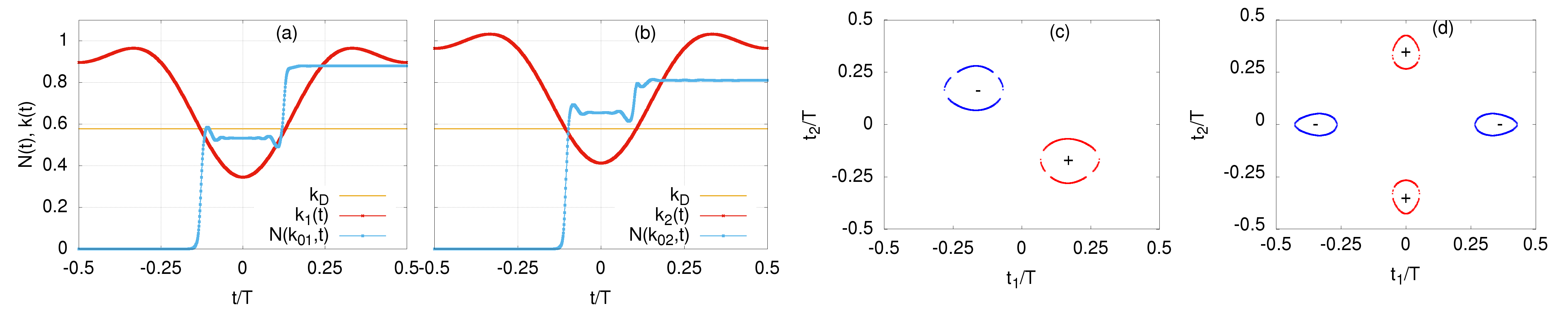
Figure 4: Particle distribution function $\mathcal{N}\left(\mathbf{k},t\right)$ at the interaction with a single cycle sine-pulse ($\phi_{\mathrm{CEP}}=\pi/2$) versus time for particular crystal momentum $\overline{\mathbf{k}}_{0}\mathbf{=}\left(k_{x}/k_{b},k_{y}/k_{b}\right)$: (a) $\overline{\mathbf{k}}_{0}\mathbf{=}\left(0.9,-0.033\right)\$and (b) $\overline{\mathbf{k}}\mathbf{=}\left(0.96,0.025\right)$. In these figures, the x-component of kinetic momentum $\mathbf{k}\left(t\right)=\mathbf{k}_{0}+\mathbf{A}$ along with Dirac point momentum ($k_{D}/k_{b}=1/\sqrt{3}$) are also plotted. All plotted quantities are dimensionless. In (c) and (d) the roots of Eqs. (23) and (25) are plotted for cosine and sine pulses, respectively. The fundamental frequency is $\omega_{0}=0.2\ \mathrm{eV}/\hbar$ and the wave-particle interaction parameter is taken to be $\chi_{0}=4$ (intensity $1.4\ \mathrm{TW/cm}^{2}$).

A typical coherent dynamics of graphene-charged carriers exposed to an intense few-cycle linearly polarized laser pulse is shown in Fig. 3. The laser field is polarized along $\Gamma-K$ direction (x-axis). In this figure particle distribution function $\mathcal{N}\left(\mathbf{k},t\right)$ at various time instances during the interaction with the two and single-cycle laser pulse is shown in reduced BZ. As indicated in this figure one can trace the correlation between excitation patterns and time dependence of the vector potential (Fig. 2). In particular, for sine pulses, cf. first and third rows, thanks to the preferred direction of the vector potential (cf. Fig. 2), one of the valleys is eventually populated. For cosine pulses, cf. second and fourth rows, despite the valley polarization during the first half of the laser pulse, the balance is recovered in the second half of the laser pulse. Note that this picture of valley polarization works only when the polarization of the laser is along $\Gamma-K$ direction and it is of a threshold nature: the electrons created near the one valley should pass to the opposite valley. To have a quantitatively more satisfactory explanation we need to solve analytically Eqs. (3) and (4). To this end, we omit the Coulomb and relaxation terms in Bloch equations Eqs. (3) and (4), which is justified for a few-cycle laser pulse.

Thus, the formal solution of Eq. (4) for the interband polarization can be written as:

$$\mathcal{P}(\mathbf{k}_{0},t)=i\int_{-\tau_{0}/2}^{t}dt^{\prime}e^{-iS\left(\mathbf{k}_{0},t^{\prime},t\right)}E\left(t^{\prime}\right)D_{\mathrm{tr}}\left(\mathbf{k}_{0}+\mathbf{A}\left(t^{\prime}\right)\right)$$

$$\times\left[1-2\mathcal{N}(\mathbf{k}_{0},t^{\prime})\right],$$ (17)

where

$$S\left(\mathbf{k}_{0},t^{\prime},t\right)=\int_{t^{\prime}}^{t}\left[\mathcal{E}_{eh}\left(\mathbf{k}_{0}+\mathbf{A}\left(t^{\prime\prime}\right)\right)\right]dt^{\prime\prime}$$ (18)

is the classical action. As is seen, the electron-hole creation amplitude is defined by the singularity of the transition dipole moment $D_{\mathrm{tr}}\left(\mathbf{k}_{0}\right)$ near the Dirac points. In this case due to the vanishing gap, electron-hole creation is initiated by the non-adiabatic crossing of the valence band electrons through the Dirac points Zurrón et al. (2018). In Figs. 4(a) and 4(b), we plot $\mathcal{N}(\mathbf{k}_{0},t)$ for two particular values of crystal momentum $\mathbf{k}_{0}$ along with time-dependent kinetic momentum $\mathbf{k}\left(t\right)=\mathbf{k}_{0}+\mathbf{A}\left(t\right)$. The horizontal line is the Dirac moment $1/\sqrt{3}$ in the units of $k_{b}$. As is clearly seen from Figs. 4(a) and 4(b), the excitation takes place almost instantly when the kinetic momentum approaches to Dirac point: $\mathbf{k}\left(t\right)=\mathbf{k}_{D}$. Thus, we can argue that to excite electrons at any point of BZ it is necessary, but as we will see is not sufficient to pass through the Dirac point. The non-adiabatic dynamics suggests to simplify Eq. (17) considerably. As in Ref. Zurrón et al. (2018), we model singularity of the transition dipole moment defining $D_{\mathrm{tr}}\left(\mathbf{k}_{0}\right)$ as a Dirac delta function in both valleys: $D_{\mathrm{tr}}\left(\mathbf{k}_{0}\right)=D_{0}\left(\delta\left(\mathbf{k}_{0}-\mathbf{k}_{D}\right)-\delta\left(\mathbf{k}_{0}+\mathbf{k}_{D}\right)\right)$. With this replacement in Eq. (17) we get:

$$\mathcal{P}(\mathbf{k}_{0},t)\varpropto i\sum\limits_{t_{d_{+}}}e^{-iS\left(\mathbf{k}_{0},t_{d_{+}},t\right)}E\left(t_{d_{+}}\right)$$

$$-i\sum\limits_{t_{d_{-}}}e^{-iS\left(\mathbf{k}_{0},t_{d_{-}},t\right)}E\left(t_{d_{-}}\right),$$ (19)

where, for a given $\mathbf{k}_{0}$, $t_{d_{+}}$ and $t_{d_{-}}$ are the solution of equations:

$$\mathbf{k}_{0}=\mathbf{k}_{D}-\mathbf{A}\left(t_{d_{+}}\right),$$ (20)

$$\mathbf{k}_{0}=-\mathbf{k}_{D}-\mathbf{A}\left(t_{d_{-}}\right).$$ (21)

These equations may have several solutions. In Figs. 4(a) and 4(b) we have two solutions $t_{d_{1+}}$, $t_{d_{2+}}$. Depending on the phase difference $\delta S=S\left(\mathbf{k}_{0},t_{d_{1+}},t_{d_{2+}}\right)$ we will have constructive or destructive interference. Thus, we can argue that to excite electrons at any point of BZ it is necessary and sufficient to pass through the Dirac point with constructive interference of multiple passages. This finding explains interference patterns in Fig. 3. Now let us calculate the electron populations around respective valleys with the same ansatz. With the help of Eq. (17), from Eq. (3) we have

$$N_{+}(\tau_{0}/2)\varpropto\int_{-\tau_{0}/2}^{\tau_{0}/2}dt^{\prime}E^{2}\left(t^{\prime}\right)-\mathrm{Re}\sum\limits_{t_{2}}\int_{-\tau_{0}/2}^{\tau_{0}/2}dt_{1}E\left(t_{1}\right)$$

$$\times E\left(t_{2}\right)e^{iS\left(\mathbf{k}_{D}-\mathbf{A}\left(t_{1}\right),t_{2},t_{1}\right)}$$ (22)

where for the given $t_{1}$, $t_{2}$ is defined from equation

$$\mathbf{A}\left(t_{2}\right)-\mathbf{A}\left(t_{1}\right)=-2\mathbf{k}_{D}.$$ (23)

Analogously we have

$$N_{-}(\tau_{0}/2)\varpropto\int_{-\tau_{0}/2}^{\tau_{0}/2}dt^{\prime}E^{2}\left(t^{\prime}\right)-\mathrm{Re}\sum\limits_{t_{2}}\int_{-\tau_{0}/2}^{\tau_{0}/2}dt_{1}E\left(t_{1}\right)$$

$$\times E\left(t_{2}\right)e^{iS\left(-\mathbf{k}_{D}-\mathbf{A}\left(t_{1}\right),t_{2},t_{1}\right)}$$ (24)

with

$$\mathbf{A}\left(t_{2}\right)-\mathbf{A}\left(t_{1}\right)=2\mathbf{k}_{D},$$ (25)

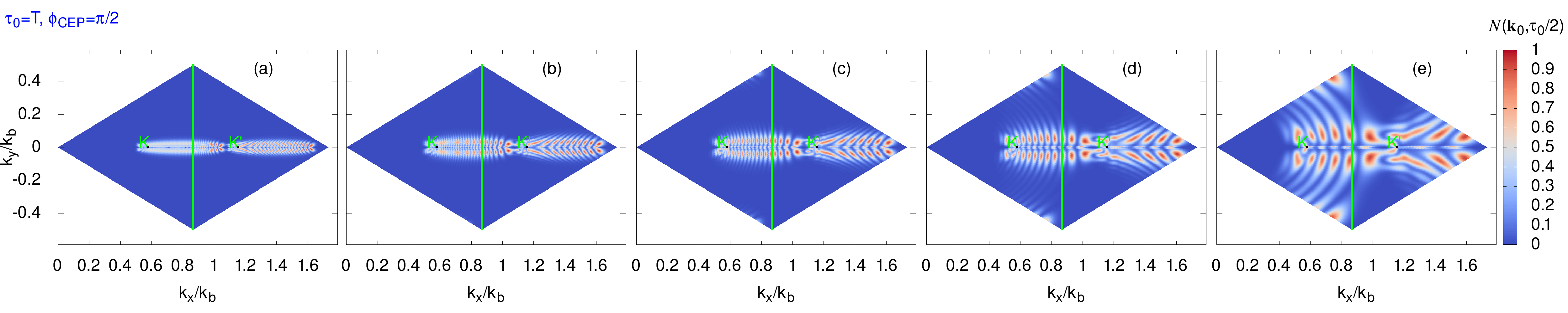
Figure 5: Particle distribution function $\mathcal{N}\left(\mathbf{k},t\right)$ (in arbitrary units) at the end of the interaction with a single cycle sine-pulse ($\phi_{\mathrm{CEP}}=\pi/2$) for graphene, as a function of scaled dimensionless momentum components ($k_{x}/k_{b}$, $k_{y}/k_{b}$). The wave-particle interaction parameter is taken to be $\chi_{0}=3.5$. (a) for $\omega_{0}=0.1\ \mathrm{eV}/\hbar$, (b) for $\omega_{0}=0.2\ \mathrm{eV}/\hbar$, (c) for $\omega_{0}=0.3\ \mathrm{eV}/\hbar$, (d) for $\omega_{0}=0.5\ \mathrm{eV}/\hbar$, and (e) for $\omega_{0}=1.0\ \mathrm{eV}/\hbar$.

As is seen from Eqs. (22) and (24) for both valleys there is a term which is defined by the intensity area of the pulse. Then we have a terms which are nonzero when electrons created near the one Dirac point reach other Dirac point in the momentum space. This explain the threshold nature of the valley polarizations. The solution of Eqs. (23) and (25) are deployed in Fig. 4(c) and 4(d) for the cosine and sine pulses, respectively. As is seen for cosine pulse if $\left(t_{1},t_{2}\right)$ pair is the solution, then we have time reversal solutions $\left(-t_{1},-t_{2}\right)$ and from $\mathcal{E}_{eh}\left(\mathbf{k}_{0}\right)=\mathcal{E}_{eh}\left(-\mathbf{k}_{0}\right)$ follows $S\left(\mathbf{k}_{D}-\mathbf{A}\left(t_{1}\right),t_{2},t_{1}\right)=-S\left(-\mathbf{k}_{D}-\mathbf{A}\left(-t_{1}\right),-t_{2},-t_{1}\right)$ and we get $N_{+}(\tau_{0}/2)=N_{-}(\tau_{0}/2)$. That is, valley polarization is zero. The same arguments can be made for infinite pulses as well. For the sine pulse the solutions for the two valleys Fig. 4(d) are not symmetric and $N_{+}(\tau_{0}/2)\neq N_{-}(\tau_{0}/2)$.

Having established the excitation dynamics of BZ with the singular transition dipole moment that works primarily along the $\Gamma-K$ direction, we next turn to the examination of excitation dynamics in the perpendicular direction. To this end, we consider the excitation of BZ with a single cycle sine-pulse ($\phi_{\mathrm{CEP}}=\pi/2$) of the same interaction parameter $\chi_{0}$ but at different frequencies. In Fig. 5, the particle distribution function $N\left(\mathbf{k},\tau_{0}/2\right)$ at the end of the interaction is shown in reduced BZ for various frequencies. As indicated in this figure, one can trace the correlation between the laser frequency and the excitation patterns, which for all cases have interference fringes. In particular, as the wave frequency decreases, the fringes become denser and thinner in the $y-$direction. The density of fringes is defined by the phase difference $\delta S=S\left(\mathbf{k}_{0},t_{d_{1+}},t_{d_{2+}}\right)$ of Eq. (19) considered above. For the given $\chi_{0}$ the phase difference $\delta S$ is inversely proportional to $\omega_{0}$, which explains the dependence of the number of fringes on the frequency. As is also clear, the excitation width in the perpendicular to laser polarization direction strongly depends on the frequency of the laser pulse. This can be understood from the x-component of the transition dipole moment, which for small $k_{y}$ near the Dirac point is $D_{\mathrm{tr}}^{(x)}\varpropto 1/\left|k_{y}\right|$. Thus, the wave-particle interaction term in Eqs. (3) and (4) is $E\left(t\right)D_{\mathrm{tr}}\varpropto\chi_{0}\omega_{0}/\left|k_{y}\right|$. Since electron-hole energy $\mathcal{E}_{eh}\varpropto\left|k_{y}\right|$, the excitation width can be estimated from the condition $\mathcal{E}_{eh}\simeq$ $E\left(t\right)D_{\mathrm{tr}}$ which gives $\left|k_{y}\right|\varpropto\sqrt{\chi_{0}\omega_{0}}$. As has been shown above, the considered setup of valley polarization works only when the polarization of the laser is along the $\Gamma-K$ direction and to have a higher degree of control one must confine the BZ excitation tighter to the $\Gamma-K$ direction. Hence, the resulting scaling $\left|k_{y}\right|\varpropto\sqrt{\chi_{0}\omega_{0}}$ indicates that low frequencies and moderate intensities are preferable for valley polarization (when the threshold condition $\chi_{0}\sim 4\pi/3$ is met).

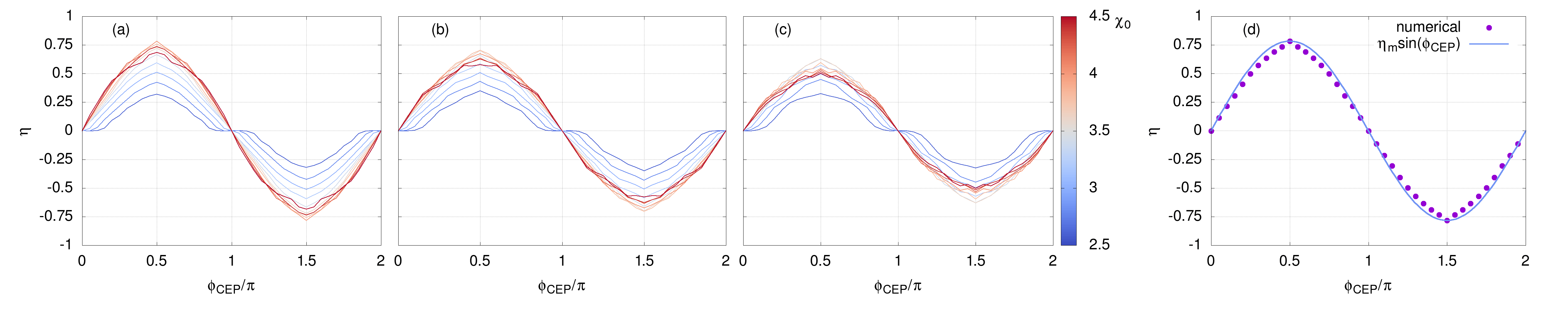
Figure 6: Valley polarization for a single-cycle linearly polarized pulse as a function of carrier-envelope phase for a range of the wave-particle interaction parameter: (a) for $\omega_{0}=0.1\ \mathrm{eV}/\hbar$, (b) for $\omega_{0}=0.2\ \mathrm{eV}/\hbar$, and (c) for $\omega_{0}=0.3\ \mathrm{eV}/\hbar$. The color box shows the strength of the wave-particle interaction parameter. The relaxation time is $\Gamma^{-1}=2\pi/\omega_{0}$. Interpolation of the valley polarization by the simple harmonic law (c) for $\omega_{0}=0.1\ \mathrm{eV}/\hbar$ and $\chi_{0}=4$.

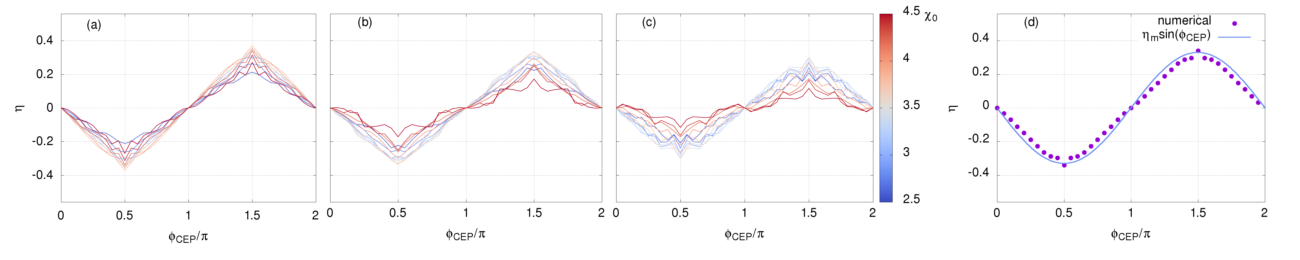
Figure 7: The same as in Fig. (6), but for a two-cycle linearly polarized pulse.

In Fig. 6 we present the results of our calculations for valley polarization in a single-cycle linearly polarized pulse as a function of carrier-envelope phase for a range of the wave-particle interaction parameter and fundamental frequency. As is seen, in single-cycle pulses we have a strong dependence of the valley polarization on CEP and we get a rather large valley polarization. For relatively smaller wave-particle interaction parameter $\chi_{0}\simeq 2.5$, the slope $d\eta/d\phi_{\mathrm{CEP}}$ of the valley polarization $\eta$ with respect to the carrier-envelope phase $\phi_{\mathrm{CEP}}$ vanishes when $\phi_{\mathrm{CEP}}/\pi$ approaches to an integer. This is the direct manifestation of the threshold nature of the considered valley polarization scheme: for a relatively smaller wave-particle interaction parameter the electrons created near the one valley do not reach the opposite valley for the range of carrier-envelope phase close to the cosine pulse. Also in Figs. 6(a), 6(b), and 6(c) we see the result of the negative factor of excitation across the $\Gamma-K$ direction (cf. Fig. 5). The scaling $\left|k_{y}\right|\varpropto\sqrt{\omega_{0}}$ indicates that the maximal amplitude of the valley polarization decreases as the fundamental frequency $\omega_{0}$ increases. Interestingly, for the wave-particle interaction parameter $\chi_{0}$ ranging from $3$ to $4$, the valley polarization $\eta$ dependence on $\phi_{\mathrm{CEP}}$ tends to harmonic law. Indeed, in Fig. 6(d) we compare the sinusoidal dependence with the numerically exact result and obtain fairly good interpolation. Note that these calculations have been made including relaxation and many-body Coulomb interaction. With the increase of the pulse duration in Fig. 7, the asymmetric parts in Eqs. (22) and ((24) become smaller and valley polarization diminished compared with a single-cycle pulse. However, the harmonic law of valley polarization versus CEP Fig. 7(d) still works. With the increase of the pulse duration in Figs. 7(a), 7(b), and especially in 7(c), where the frequency is larger, we see the negative factor of excitation across the $\Gamma-K$ direction because of scaling $\left|k_{y}\right|\varpropto\sqrt{\chi_{0}\omega_{0}}$ which implies that moderate intensities are preferable for valley polarization. We also see that along with the harmonic law of the valley polarization, there is a high-frequency amplitude modulation of the valley polarization, which becomes more pronounced near its extrema.

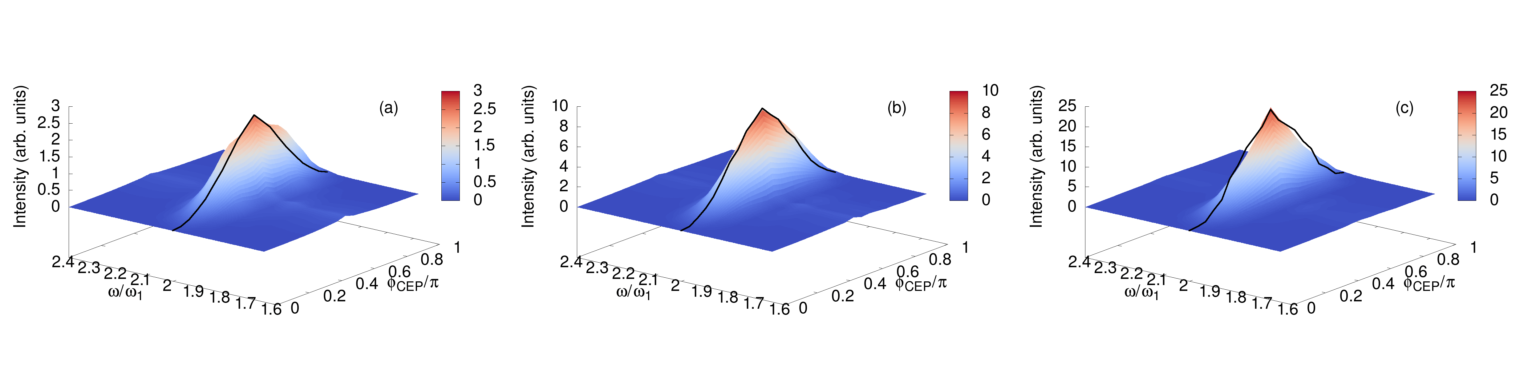
Figure 8: The nonlinear response of the graphene in a multi-cycle laser field of wavelength $800\ \mathrm{nm}$ ($\omega_{1}=1.55\ \mathrm{eV}/\hbar$) near the second harmonic via the normalized intensity versus carrier-envelope phase of a single-cycle linearly polarized preexcitation pulse: (a) for $\omega_{0}=0.1\ \mathrm{eV}/\hbar$, (b) for $\omega_{0}=0.2\ \mathrm{eV}/\hbar$, and (c) for $\omega_{0}=0.3\ \mathrm{eV}/\hbar$. The wave-particle interaction parameter for a preexcitation pulse is taken to be $\chi_{0}=3.5$, while for a multi-cycle laser field we take $\chi_{1}=0.1\chi_{0}$. The black (solid) lines over the surface plots are the second harmonic intensities calculated as $I_{2}\sim\eta^{2}\left(\phi_{\mathrm{CEP}}\right)$.

III.2 Harmonic imaging of valley polarization and CEP of few-cycle laser pulses in graphene

Having considered the coherent dynamics of graphene charge carriers subjected to intense, linearly polarized, few-cycle laser pulses, we then consider the harmonic mapping of valley polarization and CEP for such pulses. Although graphene is centrosymmetric, and as a result, there are no even-order harmonics for equilibrium initial states, it turns out that spatial dispersion or valley polarization initiates a rather large second-order nonlinear response Avetissian et al. (2020); Golub and Tarasenko (2014); Wehling et al. (2015); Ho et al. (2020), comparable to non-centrosymmetric 2D. The sensitivity of the second harmonic to valley-polarization opens a door for solving two important issues regarding the valleytronics and light wave electronics: measuring of valley-polarization and CEP which is important for manipulations with short laser pulses. Hence, in this subsection we consider harmonic generation in a multi-cycle laser field of relatively moderate intensity by graphene preliminary exposed to an intense few-cycle laser pulse.

The EM response in 2D hexagonal nanostructure is determined by the total current density:

$$\mathbf{j}\left(t\right)=-\frac{4}{(2\pi)^{2}}\int_{\widetilde{BZ}}d\mathbf{k}_{0}\left\{\mathbf{v}_{c}\left(\mathbf{k}_{0}+\mathbf{A}\right)\mathcal{N}\left(\mathbf{k}_{0},t\right)\right.$$

$$+\left.\mathrm{Re}\left[\mathbf{v}_{\mathrm{tr}}^{\ast}\left(\mathbf{k}_{0}+\mathbf{A}\right)\mathcal{P}(\mathbf{k}_{0},t)\right]\right\},$$ (26)

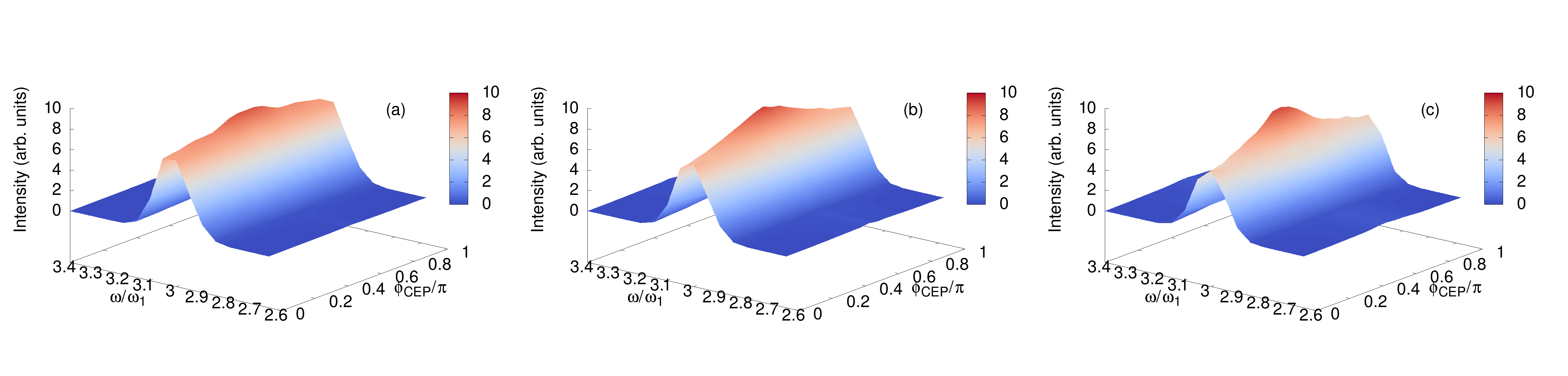
Figure 9: The same as in Fig. (8), but for a third harmonic.

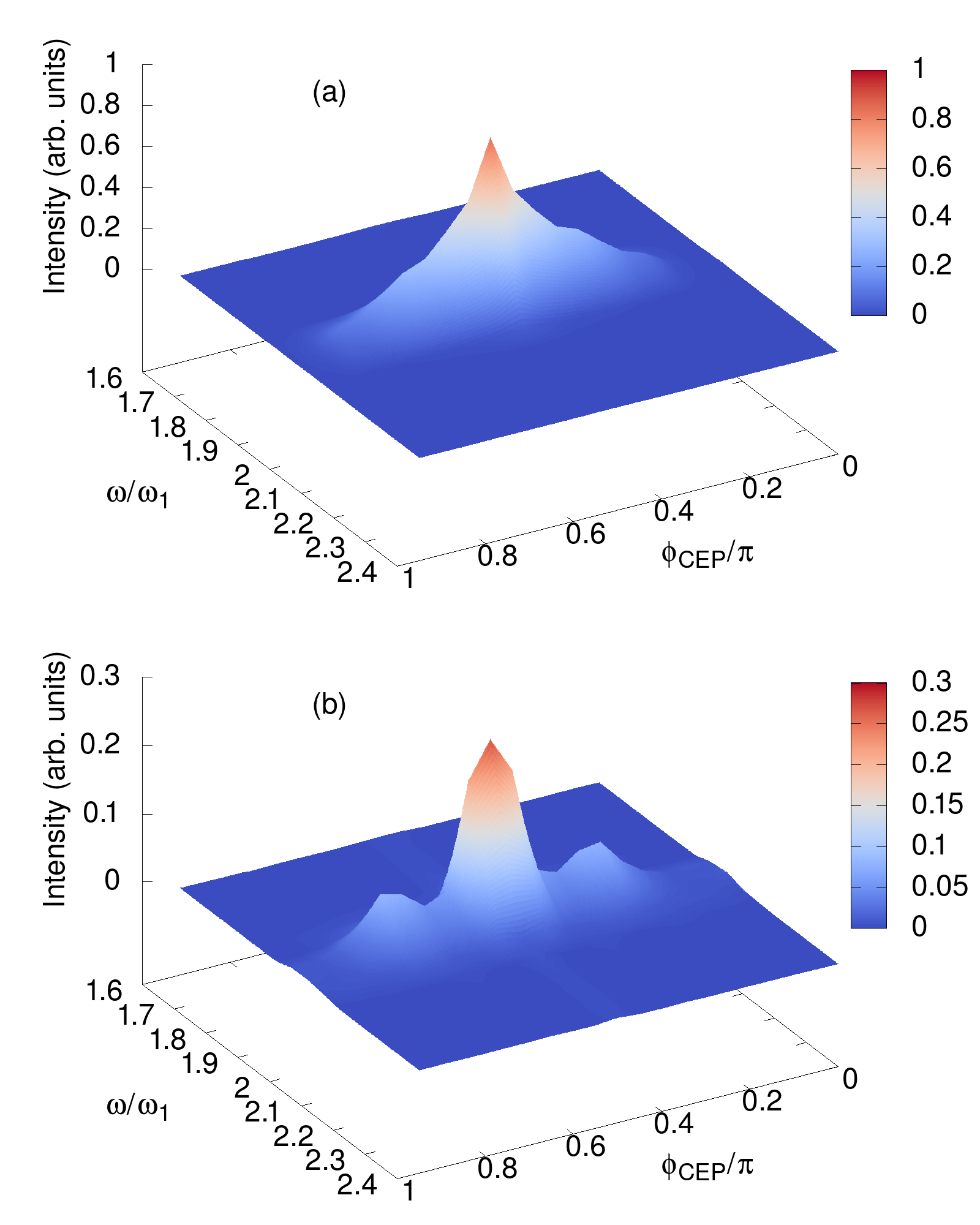
Figure 10: The nonlinear response of the graphene in a multi-cycle laser field of wavelength $800\ \mathrm{nm}$ ($\omega_{2}=1.55\ \mathrm{eV}/\hbar$) near the second harmonic via the normalized intensity versus carrier-envelope phase of a two-cycle (a) and three-cycle (b) linearly polarized preexcitation pulse. The wave-particle interaction parameters are $\chi_{0}=3.5$ and $\chi_{1}=0.1\chi_{0}$, while the fundamental frequency is $\omega_{0}=0.2\ \mathrm{eV}/\hbar$.

where the band velocity $\mathbf{v}_{c}\left(\mathbf{k}\right)=\partial E\left(\mathbf{k}\right)/\partial\mathbf{k}$ defines intraband contribution, while transition matrix element $\mathbf{v}_{\mathrm{tr}}\left(\mathbf{k}\right)=2iE\left(\mathbf{k}\right)D_{\mathrm{tr}}\left(\mathbf{k}\right)\$of the velocity defines interband contribution. The Brillouin zone is also shifted to $\widetilde{BZ}=BZ-A$. Note that for the initially dopped system one should take into account the next-nearest neighbor hopping term ($\gamma^{\prime}$) which breaks the electron-hole symmetry Kretinin et al. (2013) and can be crucial for the second harmonic generation in the presence of asymmetric Fermi energies of valleys wehling2015probing. Since we consider an undoped system in equilibrium neglecting thermal occupations, and $\gamma^{\prime}$ does not change the energy difference between the bands, the contribution from $\gamma^{\prime}$ to the total current density vanishes Kretinin et al. (2013) when the difference is computed in Eq. (26). For sufficiently large 2D sample, the generated electric field far from the hexagonal layer is proportional to the surface current: $\mathbf{E}^{(g)}(t)=-2\pi\mathbf{j}\left(t\right)/c$ Avetissian and Mkrtchian (2018). The HHG spectral intensity is calculated from the fast Fourier transform of the generated field $\mathbf{E}^{(g)}(\omega)$. Now we solve Bloch equations Eqs. (3) and (4) with the initial conditions $\mathcal{P}(\mathbf{k},0)=\mathcal{P}(\mathbf{k},\tau_{0}/2)$ and $N(\mathbf{k},0)=N(\mathbf{k},\tau_{0}/2)$, where $\mathcal{P}(\mathbf{k},\tau_{0}/2)$ and $N(\mathbf{k},\tau_{0}/2)$ are interband polarization and particle distribution function at the end of the preexcitation pulse.

In Fig. 8, the nonlinear response of the graphene in a multi-cycle laser field $\tau_{1}=40\pi/\omega_{1}$ of wavelength $800\ \mathrm{nm}$ ($\omega_{1}=1.55\ \mathrm{eV}/\hbar$) near the second harmonic via the normalized intensity versus carrier-envelope phase of a single-cycle linearly polarized preexcitation pulse is displayed for several fundamental frequencies. The wave-particle interaction parameter for a multi-cycle laser field is taken to be smaller by one order compared to the preexcitation pulse. We specifically consider spectral intensity near the second harmonic to show that the second harmonic intensity is a robust observable that provides a gauge of CEP. As is seen from these figures, the second harmonic signal vanishes for a cosine pulse $\phi_{\mathrm{CEP}}=0$ and for the sine pulse $\phi_{\mathrm{CEP}}=\pi/2$ reaches maximum values, between these values it is a monotonic function. In contrast to the second harmonic, the third harmonic is almost independent of CEP, cf. Fig. 9. That is, for diagnostic tools the second harmonic is unique. Moreover, as follows from perturbation theory Golub and Tarasenko (2014), when valley polarization is modeled via different Fermi energies in the $K$ and $K^{\prime}$ valleys, the intensity of the second harmonic is proportional to the square of valley polarization. In Fig. 8, we see that the second harmonic intensities calculated as $I_{2}\sim\eta^{2}\left(\phi_{\mathrm{CEP}}\right)\sim\sin^{2}\left(\phi_{\mathrm{CEP}}\right)$, where $\eta\left(\phi_{\mathrm{CEP}}\right)$ is from Fig. 6 fairly well coincide with the exact numerical results. Thus, for a single-cycle laser pulse we can reach controllable valley polarization, which harmonically depends on the carrier-envelope phase, and vice versa, via valley-polarization we can measure CEP which is essential for short pulse manipulations and light-wave electronics. This finding is also valid for two-cycle laser pulse Fig. 10(a). However, for three-cycle laser pulse Fig. 10(b) the second harmonic intensity is not a monotonic function in the range $\phi_{\mathrm{CEP}}\subset\left[0,\pi/2\right]$ and a simple dependence $I_{2}\sim\eta^{2}$ does not hold. This is connected with the above-mentioned fact of amplitude modulation of valley polarization: with the further increase of the pulse duration valley polarization diminished and becomes comparable to the depth of the amplitude modulation caused by excitation of BZ across the $\Gamma-K$ direction. Note that harmonic dependence essentially simplifies the possibility of measurement of valley polarization and CEP but is not mandatory for their measurement. For harmonic law one needs one triple of quantities $I_{2},\eta\rightarrow\phi_{\mathrm{CEP}}$, otherwise one needs several sets of triples for calibration.

IV Conclusion

We have investigated the coherent dynamics of graphene-charged carriers exposed to an intense few-cycle linearly polarized laser pulse. Solving the corresponding generalized semiconductor Bloch equations numerically in the Hartree-Fock approximation taking into account many-body Coulomb interaction, we demonstrated that valley polarization is strongly dependent on the CEP, which for a range of intensities can be interpolated by the simple harmonic law. The obtained numerical results are supported by approximate and transparent analytical results. Then, we have considered harmonic generation in a multi-cycle laser field by graphene pre-excited by an intense few-cycle laser pulse. The obtained results show that valley polarization and CEP have their unique footprints in the second harmonic signal, which will allow us to measure both physical quantities for pulse durations up to two optical cycles, which are vital for valleytronics and light-wave electronics.