Topological Characterization of Consensus Solvability
in Directed Dynamic Networks

Abstract

Consensus is one of the most fundamental problems in distributed computing. This paper studies the consensus problem in a synchronous dynamic directed network, in which communication is controlled by an oblivious message adversary. The question when consensus is possible in this model has already been studied thoroughly in the literature from a combinatorial perspective, and is known to be challenging. This paper presents a topological perspective on consensus solvability under oblivious message adversaries, which provides interesting new insights.

Our main contribution is a topological characterization of consensus solvability, which also leads to explicit decision procedures. Our approach is based on the novel notion of a communication pseudosphere, which can be seen as the message-passing analog of the well-known standard chromatic subdivision for wait-free shared memory systems. We further push the elegance and expressiveness of the “geometric” reasoning enabled by the topological approach by dealing with uninterpreted complexes, which considerably reduce the size of the protocol complex, and by labeling facets with information flow arrows, which give an intuitive meaning to the implicit epistemic status of the faces in a protocol complex.

1 Introduction

Consensus is a most fundamental problem in distributed computing, in which multiple processes need to agree on some value, based on their local inputs. The problem has already been studied for several decades and in various different models, yet in many distributed settings the question of when and how fast consensus can be achieved continues to puzzle researchers.

This paper studies consensus in the fundamental setting where processes communicate over a synchronous dynamic directed network, where communication is controlled by an oblivious message adversary [AG13]. This model is appealing, because it is conceptually simple and still provides a highly dynamic network model. In this model, fault-free processes communicate in a lock-step synchronous fashion using message passing, and a message adversary may drop some messages sent by the processes in each round. Viewed more abstractly, the message adversary provides a sequence of directed communication graphs, whose edges indicate which process can successfully send a message to which other process in that round. An oblivious message adversary is defined by a set $\mathbf{D}$ of allowed communication graphs, from which it can pick one in each round [CGP15], independently of its picks in the previous rounds.

The model is practically motivated, as the communication topology of many large-scale distributed systems is dynamic (e.g., due to mobility, interference, or failures) and its links are often asymmetric (e.g., in optical or in wireless networks) [NKYG07]. The model is also theoretically interesting, as solving consensus in general dynamic directed networks is known to be difficult [SW89, SWK09, CGP15, BRSSW18:TCS, WSS19:DC].

Prior work primarily focused on the circumstances under which consensus is actually solvable under oblivious message adversaries [CGP15]. Only recently, first insights have been obtained on the time complexity of reaching consensus in this model [WPRSS23:ITCS], using a combinatorial approach. The present paper complements this by a topological perspective, which provides interesting new insights and results.

Our contributions: Our main contribution is a topological characterization of consensus solvability for synchronous dynamic networks under oblivious message adversaries. It provides not only intuitive (“geometric”) explanations for the surprisingly intricate time complexity results established in [WPRSS23:ITCS], both for the decision procedure (which allows to determine whether consensus is solvable for a given oblivious message adversary or not) and, in particular, for the termination time of any correct distributed consensus algorithm.

To this end, we introduce the novel notion of a communication pseudosphere, which can be seen as the message-passing analog of the well-known standard chromatic subdivision for wait-free shared memory systems. Moreover, we use uninterpreted complexes [SC20:PODC], which considerably reduce the size and structure of our protocol complexes. And last but not least, following [GP16:OPODIS], we label the edges in our protocol complexes by the information flow that they carry, which give a very intuitive meaning to the the implicit epistemic status (regarding knowledge of initial values) of the vertices/faces in a protocol complex. Together with the inherent beauty and expressiveness of the topological approach, our tools facilitate an almost “geometric” reasoning, which provides simple and intuitive explanations for the surprising results of [WPRSS23:ITCS], like the sometimes exponential gap between decision complexity and consensus termination time. It also leads to a novel decision procedure for deciding whether consensus under a given oblivious message adversary can be achieved in some $k$ rounds.

In general, we believe that, unlike the combinatorial approaches considered in the literature so far, our topological approach also has the potential for the almost immediate generalization to other decision problems and other message adversaries, and may hence be of independent interest.

Related work: Consensus problems arise in various models, including shared memory architectures, message-passing systems, and blockchains, among others [ongaro2014search, KO11:SIGACT, WS19:EATCS, abraham2017blockchain]. The distributed consensus problem in the message-passing model, as it is considered in this paper, where communication occurs over a dynamic network, has been studied for almost 40 years [HRT02:ENTCS, SW07, SWK09, CBS09, BSW11:hyb, CGP15, CFN15:ICALP, FNS18:PODC]. Already in 1989, Santoro and Widmayer [SW89] showed that consensus is impossible in this model if up to $n-1$ messages may be lost each round. Schmid, Weiss and Keidar [SWK09] showed that if losses do not isolate the processes, consensus can even be solved when a quadratic number of messages is lost per round. Several other generalized models have been proposed in the literature [Gaf98, KS06, CBS09], like the heard-of model by Charron-Bost and Schiper [CBS09], and also different agreement problems like approximate and asymptotic consensus have been studied in these models [CFN15:ICALP, FNS18:PODC]. In many of these and similar works on consensus [FG11, BRS12:sirocco, SWS16:ICDCN, BRSSW18:TCS, WSS19:DC, NSW19:PODC, CastanedaFPRRT21topo], a model is considered in which, in each round, a digraph is picked from a set of possible communication graphs. Afek and Gafni coined the term message adversary for this abstraction [AG13], and used it for relating problems solvable in wait-free read-write shared memory systems to those solvable in message-passing systems. For a detailed overview of the field, we refer to the recent survey by Winkler and Schmid [WS19:EATCS].

An interesting alternative model for dynamic networks assumes a $T$-interval connectivity guarantee, that is, a common subgraph in the communication graphs of every $T$ consecutive rounds [KLO10:STOC, KOM11]. In contrast to our directional model, solving consensus is relatively simple here, since the $T$-interval connectivity model relies on bidirectional links and always connected communication graphs. For example, $1$-interval-connectivity, the weakest form of $T$-interval connectivity, implies that all nodes are able to reach all the other nodes in the system in each of the graphs. Solving consensus in undirected graphs that are always connected was also considered in the case of a given $(t+1)$-connected graph and at most $t$-node failures [CastanedaFPRRT19tres]. Using graph theoretical tools, the authors extend the notion of a radius in a graph to determine the consensus termination time in the presence of failures.

Coulouma, Godard, and Peters [CGP15] showed an interesting equivalence relation, which captures the essence of consensus impossibility under oblivious message adversaries via the non-broadcastability of one of the so-called beta equivalence classes, hence refining the results of [SW07]. Building upon some of these insights, Winkler et al. [WPRSS23:ITCS] studied of the time complexity of consensus in this model. In particular, they presented an explicit decision procedure and analyzed both its decision time complexity and the termination time of distributed consensus. It not only turned out that consensus may take exponentially longer than broadcasting [itcs23broadcast], but also that there is sometimes an exponential gap between decision time and termination time. Surprisingly, this gap is not caused by properties related to broadcastability of the beta classes, but rather by the number of those.

Whereas all the work discussed so far is combinatorial in nature, there is also some related topological research, see [HKR13] for an introduction and overview. Using topology in distributed computing started out from wait-free computation in shared memory systems with immediate atomic snapshots (the IIS model), see e.g. [HS99:ACT, AttiyaC13, AttiyaCHP19, Kozlov15, Kozlov16, GRS22:ITCS]. The evolution of the protocol complex in the IIS model is governed by the pivotal chromatic subdivision operation here. We will show that the latter can alternatively be viewed as a specific oblivious message adversary, the set $\mathbf{D}$ of which containins all transitively closed and unilaterally connected graphs.

Regarding topology in dynamic networks, Castañeda et al. [CastanedaFPRRT21topo] studied consensus and other problems in both static and dynamic graphs, albeit under the assumption that all the nodes know the graph sequence. That is, they focused on the question of information dissemination, and put aside questions of indistinguishability between graph sequences. In contrast, in our paper, we develop a topological model that captures both information dissemination and indistinguishability. An adversarial model that falls into “our” class of models has been considered by Godard and Perdereau [GP16:OPODIS], who studied general $k$-set agreement under the assumption that some maximum number of (bidirectional) links could drop messages in a round. The authors also introduced the idea to label edges in the protocol complex by arrows that give the direction of the information flow, which we adopted. Shimi and Castañeda [SC20:PODC] studied $k$-set agreement under the restricted class of oblivious message adversaries that are “closed-above” (with $\mathbf{D}$ containing, for every included graph, also all graphs with more edges).

One of the challenges of applying topological tools in distributed settings is that the simplicial complex representing the system grows dramatically with the number of rounds, as well as with the number of processes and possible input values. In the case of colorless tasks, such as $k$-set agreement, the attention can be restricted to colorless protocol complexes [HKR13]. In the case of the IIS model, its evolution is governed by the barycentric subdivision, which results in much smaller protocol complexes than produced by the chromatic subdivision. Unfortunately, however, it is not suitable for tracing indistinguishability in dynamic networks under message adversaries. The same is true for the “local protocol complexes” introduced in [FraigniaudP20]. By contrast, uninterpreted complexes, as introduced in [SC20:PODC], are effective here and are hence also used in our paper.

Apart from consensus being a special case of $k$-set agreement (for $k=1$), consensus has not been the primary problem of interest for topology in distributed computing, in particular not for dynamic networks under message adversaries. However, a point-set topological characterization of when consensus is possible under general (both closed and non-closed) message adversaries has been presented by Nowak, Schmid and Winkler in [NSW19:PODC]. The resulting decision procedure is quite abstact, though (it acts on infinite admissible executions), and so are some results on the termination time for closed message adversaries that confirm [WSM19:OPODIS].

The topology of message-passing models in general has been considered by Herlihy, Rajsbaum, and Tuttle already in 2002 [HRT02:ENTCS]. Herlihy and Rajsbaum [HR10] studied $k$-set agreement in models leading to shellable complexes.

Paper organization: We introduce our model of distributed computation and the oblivious message adversary in Section 2. In Section 3 we present a framework which will allow us to study consensus on dynamic networks from a topological perspective. Our characterization of consensus solvability/impossibility for the oblivious message adversary is presented in Section 4, where we also describe an explicit decision procedure. In Section LABEL:sec:terminationtime we further explore the relationship between the time complexity required by our decision procedure and the actual termination time of distributed consensus. We conclude our contribution and discuss future research directions in Section LABEL:sec:conclusion.

2 System Model

We consider a synchronous dynamic network consisting of a set of $n$ processes that do not fail, which are fully-connected via point-to-point links that might drop messages. We identify the processes solely by their unique ids, which are taken from the set $\Pi=\{p_{1},\dots,p_{n}\}$ and known to the processes. Let $[n]=\{1,\dots,n\}$. Processes execute a deterministic full-information protocol $P$, using broadcast (send-to-all) communication. Their execution proceeds in a sequence of lock-step rounds, where every process simultaneously broadcasts a message to every other process, without getting immediately informed of a successful message reception, and then computes its next state based on its current local state and the messages received in the round. The rounds are communication-closed, i.e., messages not received in a specific round are lost and will not be delivered later.

Communication is hence unreliable, and in fact controlled by an oblivious message adversary (MA) with non-empty graph set $\mathbf{D}=\{D_{1},\dots,D_{k}\}$. All the graphs have $\Pi$ as their set of nodes, and an edge $p_{i}\to p_{j}$ represents a communication link from $p_{i}$ to $p_{j}$. For every round $r\geq 1$, the MA arbitrarily picks some communication graph $G_{r}$ from $\mathbf{D}$, and a message from a process $p_{i}$ arrives to process $p_{j}$ in this round if $G_{r}$ contains the edge $p_{i}\to p_{j}$, and otherwise it is lost. We assume processes have persistent memory, i.e., every graph in $\mathbf{D}$ contains all self-loops $p_{i}\to p_{i}$. An infinite graph sequence $\mathcal{G}=(G_{r})_{r\geq 1}$ picked by the message adversary is called a feasible graph sequence, and $\mathbf{D}^{\omega}$ denotes the set of all feasible graph sequences for the oblivious message adversary with graph set $\mathbf{D}$. The processes know $\mathbf{D}$, but they do not have a priori knowledge of the graph $G_{r}$ for any $r$ (though they may infer it after the round occurred).

We consider a system where the global state is fully determined by the local states of each process. Therefore, a configuration is just the vector of the local states (also called views) of the processes. An admissible execution $a$ of $P$ is just the sequence of configurations $a=(a_{r})_{r\geq 0}$ at the end of the rounds $r\geq 1$, induced by a feasible graph sequence $\mathcal{G}\in\mathbf{D}^{\omega}$ starting out from a given initial configuration $a_{0}$. Since we will restrict our attention to deterministic protocols $P$, the graph sequence $\mathcal{G}$ and the initial configuration $a_{0}$ uniquely determine $a$. The view of process $p_{i}$ in $a_{r}$ at the end of round $r\geq 1$ is denoted as $a_{r}(p_{i})$; its initial view is denoted as $a_{0}(p_{i})$.

We restrict our attention to deterministic protocols for the consensus problem, defined as follows:

Definition 1 (Consensus)

Every process $p_{i}\in\Pi$ has an input value $x_{i}\in\mathcal{V}_{I}$ taken from a finite input domain $\mathcal{V}_{I}$, which is encoded in the initial state, and an output value $y_{i}\in\mathcal{V}_{I}\cup\{\bot\}$, initially $y_{i}=\bot$. In every admissible execution, a correct consensus protocol $P$ must ensure the following properties:

• Termination: Eventually, every $p_{i}\in\Pi$ must decide, i.e., change to $y_{i}\neq\bot$, exactly once.

• Agreement: If processes $p_{i}$ and $p_{j}$ have decided, then $y_{i}=y_{j}$.

• (Strong) Validity: If $y_{i}\neq\bot$, then $y_{i}=x_{j}$ for some $p_{j}\in\Pi$, i.e., must be the input value of some process $p_{j}$.

In any given admissible execution $a$ of $P$, induced by $\mathcal{G}\in\mathbf{D}^{\omega}$, for a process $p_{i}$, let $\operatorname{In}^{\mathcal{G}}(p_{i},r)$ be the set of processes $p_{i}$ has heard of in round $r$ (see also [CBS09]), i.e., the set of in-neighbors of process $p_{i}$ in $G_{r}$, and $\operatorname{In}^{\mathcal{G}}(p_{i},0)=\{p_{i}\}$. Since all graphs in $\mathbf{D}$ contain all self-loops, we have that $p_{i}\in\operatorname{In}^{\mathcal{G}}(p_{i},r)$ for all $r\geq 0$ and $p_{i}\in\Pi$. If the round $r$ is clear from the context, we also abbreviate $\operatorname{In}^{\mathcal{G}}(p_{i})=\operatorname{In}^{\mathcal{G}}(p_{i},r)$.

The evolution of the local views of the processes in an admissible execution $a$, induced by $\mathcal{G}$ and the initial configuration $a_{0}$, can now be defined recursively as

$$a_{r}(p_{i})=\bigl{\{}(p_{j},r,a_{r-1}(p_{j})):p_{j}\in\operatorname{In}^{\mathcal{G}}(p_{i},r)\bigr{\}}\quad\mbox{for $r>0$}.$$ (1)

Note that we could drop the round number $r$ from $(p_{j},r,a_{r-1}(p_{j}))$ in the above definition, since it is implicitly contained in the structure of $a_{r}(p_{i})$; we included it explicitly for clarity only. The set of all possible round-$r$ views of $p_{i}$, including all the initial views for $r=0$, in any admissible execution, is denoted by $A^{r}(p_{i})=\{a_{r}(p_{i})\mid\forall\mbox{ admissible executions $a$ under MA}\}$.

In any admissible execution $a$, every process must eventually reach a final view, where it can take a decision on an output value which will not be changed later. Consequently, there is some final round after which all processes have decided.

3 A Topological Framework for Consensus

In this section, we introduce the basic elements of combinatorial topology and specific concepts needed in our context of synchronous message-passing networks.

Combinatorial topology in distributed computing [HKR13] rests on simplicial input and output complexes describing the feasible input and output values of a distributed decision task like consensus, and a carrier map that defines the allowed output value(s), i.e., output simplices, for a given input simplex. A protocol that solves such a task in some computational model gives rise to another simplicial complex, the protocol complex, which describes the evolution of the local views of the processes in any execution. Protocol complexes traditionally model full information protocols in round-based models, which ensures a well-organized structure: The processes execute a sequence of communication operations, which disseminate their complete views, until they are able to make a decision. Finally, a protocol induces a simplicial decision map, which maps each vertex in the protocol complex to an output vertex in a way compatible with the carrier map.

3.1 Basic topological definitions

We start with the definitions of the basic vocabulary of combinatorial topology:

Definition 2 (Abstract simplicial complex)

An abstract simplicial complex $\mathcal{K}$ is a pair $\langle V(\mathcal{K}),F(\mathcal{K})\rangle$, where $V(\mathcal{K})$ is a set, $F(\mathcal{K})\subseteq 2^{V(\mathcal{K})}$, and for any $\sigma,\tau\in 2^{V(\mathcal{K})}$ such that $\sigma\subseteq\tau$ and $\tau\in F(\mathcal{K})$, then $\sigma\in F(\mathcal{K})$. $V(\mathcal{K})$ is called the set of vertices, and $F(\mathcal{K})$ is the set of faces or simplices of $\mathcal{K}$. We say that a simplex $\sigma$ is a facet if it is maximal with respect to containment, and a proper face otherwise. We use $Fct(\mathcal{K})$ to denote the set of all facets of $\mathcal{K}$, and note that for a given $V(\mathcal{K})$ we have that $F(\mathcal{K})$ uniquely define $Fct(\mathcal{K})$ and vice versa. A simplicial complex is finite if its vertex set is finite, which will be the case for all the complexes in this paper.

All the simplicial complexes we consider in this work are abstract. For conciseness, we will usually sloppily write $\sigma\in\mathcal{K}$ instead of $\sigma\in F(\mathcal{K})$.

Definition 3 (Subcomplex)

Let $\mathcal{K}$ and $\mathcal{L}$ be simplicial complexes. We say that $\mathcal{L}$ is a subcomplex of $\mathcal{K}$, written as $\mathcal{L}\subseteq\mathcal{K}$, if $V(\mathcal{L})\subseteq V(\mathcal{K})$ and $F(\mathcal{L})\subseteq F(\mathcal{K})$.

Definition 4 (Dimension)

Let $\mathcal{K}$ be a simplicial complex, and $\sigma\in F(\mathcal{K})$ be a simplex. We say that $\sigma$ has dimension $k$, denoted by $\dim(\sigma)=k$, if it has a cardinality of $k+1$. A simplicial complex $\mathcal{K}$ is of dimension $k$ if every facet has dimension at most $k$, and it is pure if all its facets have the same dimension.

We sometimes denote a simplex as $\sigma^{k}$ in order to stress that its dimension is $k$.

Definition 5 (Skeletons and boundary complex)

The $k$-skeleton $\operatorname{skel}^{k}(\mathcal{K})$ of a simplicial complex $\mathcal{K}$ is the subcomplex consisting of all simplices of dimension at most $k$. The boundary complex $\partial\sigma$ of a simplex $\sigma$, viewed as a complex, is the complex made up of all proper faces of $\sigma$.

Definition 6 (Simplicial maps)

Let $\mathcal{K}$ and $\mathcal{L}$ be simplicial complexes. We say that a vertex map $\mu:V(\mathcal{K})\rightarrow V(\mathcal{L})$ is a simplicial map if, for any $\sigma\in F(\mathcal{K})$, $\mu(\sigma)\in F(\mathcal{L})$; here, $\mu(\sigma)=\{\mu(v)\mid v\in\sigma\}$.

Definition 7 (Colorings and chromatic simplicial complexes)

We say that a simplicial complex $\mathcal{K}$ has a proper $c$-coloring $\chi$, if there exists $\chi:V(\mathcal{K})\to\{p_{1},p_{2},\ldots,p_{c}\}$ that is injective at every face of $\mathcal{K}$. If $\mathcal{K}$ has a proper $(\dim(\mathcal{K})+1)$-coloring, we say it is a chromatic simplicial complex.

The range of $\chi$ is extended to sets of vertices $S$ by defining $\chi(S)=\{\chi(v)\mid v\in S\}$, which implies e.g. $\chi(\sigma)=\chi(V(\sigma))$.

Definition 8 (Carrier Map)

Let $\mathcal{K}$ and $\mathcal{L}$ be simplicial complexes and $\Phi:F(\mathcal{K})\rightarrow 2^{\mathcal{L}}$. We say that $\Phi$ is a carrier map, if $\Phi(\sigma)$ is a subcomplex of $\mathcal{L}$ for any $\sigma\in\mathcal{K}$, and for any $\sigma_{1},\sigma_{2}\in\mathcal{L}$, $\Phi(\sigma_{1}\cap\sigma_{2})\subseteq\Phi(\sigma_{1})\cap\Phi(\sigma_{2})$.

We say that a carrier map is rigid if it maps every simplex $\sigma\in\mathcal{K}$ to a complex $\Phi(\sigma)$ which is pure of dimension $\dim(\sigma)$. It is said to be strict if that for any two simplices $\sigma,\tau\in\mathcal{K}$, $\Phi(\sigma\cap\tau)=\Phi(\sigma)\cap\Phi(\tau)$.

We say that a carrier map $\Phi:\mathcal{K}\rightarrow 2^{\mathcal{L}}$ carries a simplicial vertex map $\mu:V(\mathcal{K})\rightarrow V(\mathcal{L}$) if for any $\sigma\in\mathcal{K}$, $\mu(\sigma)\in\Phi(\sigma)$.

Having introduced our basic vocabulary, we can now define the main ingredients for the topological modeling of consensus in our setting.

Generally, a distributed task is defined by a tuple $T=\langle\mathcal{I},\mathcal{O},\Delta\rangle$ consisting of chromatic simplicial complexes $\mathcal{I}$ and $\mathcal{O}$ that model the valid input and output configurations respectively, for the set $\Pi$ of processes, and $\Delta:\mathcal{I}\rightarrow 2^{\mathcal{O}}$ is a carrier map that maps valid input configurations to sets of valid output configurations. Both complexes have vertices of the form $(p_{i},x)$ with $p_{i}\in\Pi$, and they are chromatic with the coloring function $\chi((p_{i},x))=p_{i}$. All the simplicial maps we consider in this work are color preserving, in the sense that they map each vertex $(p_{i},x)$ to a vertex $(p_{i},y)$ with the same process id $p_{i}$.

Many interesting tasks have some degree of regularity (that is, symmetry) in the input complex. In the case of consensus, in particular, any combination of input values from $\mathcal{V}_{I}$ is a legitimate initial configuration. Consequently, the input complex for consensus in the classic topological modeling is a pseudosphere [HRT02:ENTCS].

In this paper, we will exploit the fact that strong validity does not force us to individually trace the evolution of every possible initial configuration of the protocol complex. We will therefore restrict our attention to uninterpreted complexes [SC20:PODC]: Instead of providing different vertices for every possible value of $x_{i}$, we provide only one vertex labeled with $\{p_{i}\}$, carrying the meaning of “the actual input value $x_{i}$ of $p_{i}$”. This way, we can abstract away the input domain $\mathcal{V}_{I}$ as well as the actual assignment of initial values $x_{i}\in\mathcal{V}_{I}$ to the processes. Topologically, uninterpreted complexes thus correspond to a “flattening” of the standard complexes with respect to all input and output values. The main advantages of resorting to uninterpreted protocol complexes is that they are exponentially smaller than the standard protocol complex, even in the case of binary consensus, and independent of the particular initial configuration. This can be compared with the study of colorless tasks [HKR13, Ch. 4], where a different form of “flattening” of the complexes is done by omitting the process ids.

Definition 9 (Uninterpreted input complex for consensus)

The uninterpreted input complex $\mathcal{I}$ for consensus is just a single initial simplex $\sigma_{0}=\{(p_{1},\{p_{1}\}),\dots,(p_{n},\{p_{n}\})\}$ and all its faces, with the set of vertices $V(\mathcal{I})=V(\sigma_{0})=\{(p_{i},\{p_{i}\})\;|\;p_{i}\in\Pi\}$, where the label $\{p_{i}\}$ represents the “uninterpreted” (i.e., fixed but arbitrary) input value of $p_{i}$.

We use $\sigma_{0}$ throughout this paper to denote the above input simplex.

The uninterpreted output complex $\mathcal{O}$ for consensus just specifies the process whose input value will determine the decision value.

Definition 10 (Uninterpreted output complex for consensus)

The uninterpreted output complex $\mathcal{O}$ for consensus is the union of $n$ disjoint complexes $\mathcal{O}(p_{j})$, $p_{j}\in\Pi$, each consisting of the simplex $\{(p_{1},\{p_{j}\}),\dots,(p_{n},\{p_{j}\})\}$ and all its faces. The label $\{p_{j}\}$ represents the “uninterpreted” (i.e., fixed but arbitrary) input value of $p_{j}$.

The carrier map $\Delta$ for the consensus task maps any face $\rho$ of the initial simplex $\sigma_{0}\in\mathcal{I}$ to $\dim(\rho)$-faces of $\mathcal{O}$ that all have a coloring equal to $\chi(\rho)$. Clearly, $\Delta$ is rigid and strict.

The uninterpreted protocol complex $\mathcal{P}_{r}^{\mathbf{D}^{\omega}}$ consists of vertices that are labeled by the heard-of histories the corresponding process has been able to gather so far.

Definition 11 (Heard-of histories)

For a feasible graph sequence $\mathcal{G}$, the heard-of history $h_{r}^{\mathcal{G}}(p_{i})$ of a process $p_{i}$ at the end of round $r$ is defined as

$$h_{r}^{\mathcal{G}}(p_{i}) = \{(p_{j},h_{r-1}^{\mathcal{G}}(p_{j}))\mid p_{j}\in\operatorname{In}^{\mathcal{G}}(p_{i},r)\}\mbox{ for $r\geq 1$},$$ (2)

$$h_{0}^{\mathcal{G}}(p_{i}) = \{p_{i}\}.$$ (3)

The global heard-of history $h_{r}^{\mathcal{G}}$ at the end of round $r$ is just the tuple $(h_{r}^{\mathcal{G}}(p_{1}),\dots,h_{r}^{\mathcal{G}}(p_{n}))$.

The set of processes $p_{i}$ has ever heard of up to $h_{r}^{\mathcal{G}}(p_{i})$, i.e., the end of round $r$, is denoted $\cup h_{r}^{\mathcal{G}}(p_{i})=\bigcup_{p_{j}\in\operatorname{In}^{\mathcal{G}}(p_{i},r)}\cup h_{r-1}^{\mathcal{G}}(p_{j})$ and $\cup h_{0}^{\mathcal{G}}(p_{i})=h_{0}^{\mathcal{G}}(p_{i})=\{p_{i}\}$.

The set of all possible heard-of histories of $p_{i}$ (resp. the global ones) at the end of round $r\geq 0$, in every feasible graph sequence $\mathcal{G}\in\mathbf{D}^{\omega}$, is denoted by

$$H^{r}(p_{i}) = \{h_{r}^{\mathcal{G}}(p_{i})\mid\mathcal{G}\in\mathbf{D}^{\omega}\},$$ (4)

$$H^{r} = \{(h_{r}^{\mathcal{G}}(p_{1}),\dots,h_{r}^{\mathcal{G}}(p_{n}))\mid\mathcal{G}\in\mathbf{D}^{\omega}\}.$$ (5)

The uninterpreted protocol complex $\mathcal{P}_{r}^{\mathbf{D}^{\omega}}$, which does not depend on the initial configuration but only on $\mathbf{D}^{\omega}$, is defined as follows:

Definition 12 (Uninterpreted protocol complex for $\mathbf{D}^{\omega}$)

The uninterpreted $r$-round protocol complex $\mathcal{P}_{r}^{\mathbf{D}^{\omega}}=\langle V(\mathcal{P}_{r}^{\mathbf{D}^{\omega}}),F(\mathcal{P}_{r}^{\mathbf{D}^{\omega}})\rangle$, $r\geq 0$, for a given oblivious message adversary $\mathbf{D}^{\omega}$, is defined by its vertices and facets as follows:

$$V(\mathcal{P}_{r}^{\mathbf{D}^{\omega}}) = \bigl{\{}(p_{i},h_{r}(p_{i}))\;|\;p_{i}\in\Pi,\;h_{r}(p_{i})\in H^{r}(p_{i})\bigr{\}},$$

$$Fct(\mathcal{P}_{r}^{\mathbf{D}^{\omega}}) = \bigl{\{}\{(p_{1},h_{r}(p_{1})),\dots,(p_{n},h_{r}(p_{n}))\}|\forall 1\leq i\leq n:p_{i}\in\Pi,(h_{r}(p_{1}),\dots,h_{n}(p_{n}))\in H^{r}\bigr{\}}.$$

For conciseness, we will often omit the superscript $\mathbf{D}^{\omega}$ when the oblivious message adversary considered is clear from the context.

The decision map $\mu:V(\mathcal{P}_{r}^{\mathbf{D}^{\omega}})\rightarrow V(\mathcal{O})$ is a chromatic simplicial map that maps a final view of a process $p_{i}$ at the end of round $r$ to an output value $p_{j}$ such that $p_{j}\in\cup h_{r}^{\mathcal{G}}(p_{i})$; it is not defined for non-final views. Note that $\mu$ is uniquely determined by the images of the facets in $\mathcal{P}_{r}^{\mathbf{D}^{\omega}}$ after any round $r$ were all processes have final views. We say that consensus is solvable if such a simplicial map $\mu$ exists.

Remark.

Standard topological modeling, which does not utilize uninterpreted complexes, also requires an execution carrier map $\Xi:\mathcal{I}\to 2^{\mathcal{P}}$, which defines the subcomplex $\Xi(\sigma)$ of the protocol complex $\mathcal{P}$ that arises when the protocol starts from the initial simplex $\sigma\in\mathcal{I}$. Solving a task requires $\mu\circ\Xi$ to be carried by $\Delta$, i.e., $\mu(\Xi(\sigma))\in\Delta(\sigma)$ for all $\sigma\in\mathcal{I}$. In our setting, since we have only one (uninterpreted) facet in our input complex $\sigma_{0}$ and a protocol complex that can be written as $\bigcup_{r\geq 1}\mathcal{P}_{r}^{\mathbf{D}^{\omega}}=\bigcup_{r\geq 1}\mathcal{P}^{r}(\sigma_{0})$ (i.e., the union of all iterated protocol complex construction operators $\mathcal{P}^{r}$ given in Definition 14 below), both the execution carrier map $\Xi$ and the carrier map $\Delta$ are independent of the actual initial values and hence quite simple: The former is just $\Xi=\bigcup_{r\geq 1}\mathcal{P}^{r}$ (with every $\mathcal{P}^{r}$ viewed as a carrier map), the latter has been stated after Definition 10.

3.2 Communication pseudospheres

Rather than directly using Definition 12 for $\mathcal{P}_{r}$, we will now introduce an alternative definition based on communication pseudospheres. The latter can be seen as the the message-passing analogon of the well-known standard chromatic subdivision (see Definition 16) for wait-free shared memory systems. Topologically, it can be defined as follows:

Definition 13 (Communication pseudosphere)

Let $\mathcal{K}$ be an $(n-1)$-dimensional pure simplicial complex with a proper coloring $\chi:V(\mathcal{K})\rightarrow\{p_{1},\ldots,p_{n}\}$. We define the communication pseudosphere $\operatorname{Ps}(\mathcal{K})$ through its vertex set and facets as follows:

$$V(\operatorname{Ps}(\mathcal{K})) =\bigl{\{}(p_{i},\sigma)\;|\;\sigma\in F(\mathcal{K}),p_{i}\in\chi(\sigma)\bigr{\}},$$ (6)

$$Fct(\operatorname{Ps}(\mathcal{K})) =\bigl{\{}\{(p_{1},\sigma_{1}),(p_{2},\sigma_{2}),\ldots(p_{n},\sigma_{n})\}\;|\;\forall 1\leq i\leq n:\;\sigma_{i}\in F(\mathcal{K}),p_{i}\in\chi(\sigma_{i})\bigr{\}}.$$ (7)

Given an $(n-1)$-dimensional simplex $\sigma^{n-1}=\{(p_{1},h_{1}),\dots,(p_{n},h_{n})\}\in\mathcal{K}$, the communication pseudosphere $\operatorname{Ps}(\sigma^{n-1})$ contains a vertex $(p_{i},\sigma)$ for every subset $\sigma\subseteq\{(p_{1},h_{1}),\dots,(p_{n},h_{n})\}$ that satisfies $\{(p_{i},h_{i})\}\in\sigma$. Intuitively, $\sigma$ represents the information of those processes $p_{i}$ could have heard of in a round (recall that $p_{i}$ always hears of itself). $\operatorname{Ps}(\sigma^{n-1})$ hence indeed matches the definition of a pseudosphere [HRT02:ENTCS].

Since $\bigl{|}\bigl{\{}\sigma\subseteq\{(p_{1},h_{1}),\dots,(p_{n},h_{n})\}\setminus\{(p_{i},h_{i})\}\bigr{\}}\bigr{|}=2^{n-1}$ for every $p_{i}$, every communication pseudosphere $\operatorname{Ps}(\sigma^{n-1})$ consists of $|V(\operatorname{Ps}(\sigma^{n-1}))|=n2^{n-1}$ vertices: For every given vertex $(p_{i},\sigma)$ and every $p_{j}\neq p_{i}$, there are exactly $2^{n-1}$ differently labeled vertices $(p_{j},\cdot)$. Since $(p_{i},\sigma)$ has an edge to each of those in the complex $\operatorname{Ps}(\sigma^{n-1})$, its degree must hence be $d=(n-1)2^{n-1}$.

In the case of $n=2$ or $n=3$, let $v=|V(\operatorname{Ps}(\sigma^{n-1}))|$, $e=|E(\operatorname{Ps}(\sigma^{n-1}))|$ and $f=|Fct(\operatorname{Ps}(\sigma^{n-1}))|$ denote the numbers of vertices, edges and facets in $\operatorname{Ps}(\sigma^{n-1})$, respectively. It obviously holds that $v\cdot d=2e$ and $v\cdot d=nf$. Therefore, $e=vd/2=n(n-1)2^{2(n-1)-1}$ and $f=vd/n=(n-1)2^{2(n-1)}$. For $n=2$, we thus get $v=4$, $f=e=4$, $d=2$ and hence the following communication pseudosphere $\operatorname{Ps}(\sigma_{0}^{1})$ for the initial simplex $\sigma_{0}^{1}=\{(p_{r},\{p_{r}\}),(p_{w},\{p_{w}\})\}$:

(8)

In the above figure, and throughout this paper, we use the labeling convention of the edges proposed in [GP16:OPODIS], which indicates the information flow between the vertices in a simplex. For example, in the middle simplex (connected with edge $\leftrightarrow$), both processes have heard from each other in round 1, so the connecting edge is denoted by $\leftrightarrow$. An edge without any arrow means that the two endpoints do not hear from each other. Note carefully that we will incorporporate these arrows also when talking about facets and faces that are isomorphic: Throughout this paper, two faces $\sigma$ and $\kappa$ arising in our protocol complexes will be considered isomorphic only if $\chi(\sigma)=\chi(\kappa)$ and if all edges have the same orientation.

We note also that the labeling of the vertices with the faces of $\sigma_{0}^{1}$ is highly redundant. We will hence condense vertex labels when we need to refer to them explicitly, and e.g. write $(p_{r},\{p_{r},p_{w}\})$ instead of $(p_{r},\{(p_{r},\{p_{r}\}),(p_{w},\{p_{w}\})\})$.

The communication pseudosphere $\operatorname{Ps}(\sigma_{0}^{2})$ for the initial simplex $\sigma_{0}^{2}=\{(p_{r},\{p_{r}\}),(p_{g},\{p_{g}\}),(p_{w},\{p_{w}\})\}$ for $n=3$ is depicted in Fig. 1. It also highlights two facets, corresponding to the graphs $G_{1}$ (grey) and $G_{2}$ (yellow):

(9)

Figure 1: Communication pseudosphere $\operatorname{Ps}(\sigma^{n-1})$ for $n=3$ (where $L=4$, $V=12$, $E=48$, $F=32$ and $d=8$), with the communication graphs of Eq. 9 highlighted. Thick edges represent the standard chromatic subdivision $\operatorname{Ch}(\sigma^{2})$.

We will now recast the definition of the uninterpreted protocol complex for a given oblivious message adversary $\mathbf{D}^{\omega}$ in terms of a communication pseudosphere. Recall from Definition 12 that the uninterpreted initial protocol complex $\mathcal{P}_{0}=\mathcal{P}_{0}^{\mathbf{D}^{\omega}}$ only consists of the single initial simplex $\sigma_{0}=\sigma_{0}^{n-1}=\{(p_{1},\{p_{1}\}),\dots,(p_{n},\{p_{n}\})\}$ and all its faces. It represents the uninterpreted initial state, where every process has heard only from itself. Here is an example for $n=3$ and $\Pi=\{p_{w},p_{r},p_{g}\}$:

(10)

Consequently, the single-round protocol complex $\mathcal{P}_{1}=\mathcal{P}_{1}^{\mathbf{D}^{\omega}}$ is just the subcomplex of the communication pseudosphere $\operatorname{Ps}(\sigma_{0})$ induced by the set $\mathbf{D}$ of possible graphs. For example, $\mathcal{P}_{1}$ for $\mathbf{D}=\{G_{1},G_{2}\}$ is the subcomplex of $\operatorname{Ps}(\sigma_{0})$ made up by the two highlighted facets corresponding to the graphs $G_{1}$ and $G_{2}$ in Fig. 1. That is, rather than labeling the vertices of $\operatorname{Ps}(\sigma_{0})$ with all the possible subsets of faces of $\sigma_{0}$ as in Definition 13, only those faces that are communicated via one of the graphs in $\mathbf{D}$ are used by the protocol complex construction operator $\mathcal{P}=\mathcal{P}^{\mathbf{D}^{\omega}}$ for generating $\mathcal{P}_{1}=\mathcal{P}(\sigma_{0})$. Conversely, if one interprets $\mathbf{D}$ as an $(n-1)$-dimensional simplicial complex $\mathbf{D}(\sigma_{0})$, consisting of one facet (and all its faces) per graph $G\in\mathbf{D}$ according to (7), one could write $\mathcal{P}^{\mathbf{D}^{\omega}}(\sigma_{0})=\operatorname{Ps}(\sigma_{0})\cap\mathbf{D}(\sigma_{0})$.

This can be compactly summarized in the following definition:

Definition 14 (Protocol complex construction pseudosphere)

Let $\mathcal{K}$ be an $(n-1)$-dimensional pure simplicial complex with a proper coloring $\chi:V(\mathcal{K})\rightarrow\{p_{1},\ldots,p_{n}\}$, and $\operatorname{In}^{G}(p_{i})$ be the set of processes that $p_{i}$ hears of in the communication graph $G\in\mathbf{D}$. We define the protocol complex construction pseudosphere $\mathcal{P}(\mathcal{K})$ for the message adversary $\mathbf{D}^{\omega}$, induced by the operator $\mathcal{P}:Fct(\mathcal{K})\to\mathcal{P}(\mathcal{K})$ that can be applied to the facets of $\mathcal{K}$, through its vertex set and facets as follows:

$$V(\mathcal{P}(\mathcal{K})) =\bigl{\{}(p_{i},\sigma)\in\Pi\times F(\mathcal{K})\;|\;\exists G\in\mathbf{D}:\operatorname{In}^{G}(p_{i})=\chi(\sigma)\bigr{\}},$$ (11)

$$Fct(\mathcal{P}(\mathcal{K})) =\bigl{\{}\{(p_{1},\sigma_{1}),\ldots,(p_{n},\sigma_{n})\}\;|\;\exists G\in\mathbf{D},\forall 1\leq i\leq n:\operatorname{In}^{G}(p_{i})=\chi(\sigma_{i})\bigr{\}}.$$ (12)

According to Definition 14, our operator $\mathcal{P}$ (as well as $\operatorname{Ps}$) is actually defined only for the facets in $\mathcal{K}$, i.e., the dimension $n-1$ is actually implicitly encoded in the operator. We will establish below that this is sufficient for our purposes, since every $\mathcal{P}$ is boundary consistent: This property will allow us to uniquely define $\mathcal{P}$ for proper faces in $\mathcal{K}$ as well. We will use the following simple definition of boundary consistency, which makes use of the fact that the proper coloring of the vertices of a chromatic simplicial complex defines a natural ordering of the vertices of any of its faces.

Definition 15 (Boundary consistency)

We say that a protocol complex construction operator $\mathcal{P}$ according to Definition 14 is boundary consistent, if for all possible choices of three facets $\sigma$, $\kappa$ and $\tau$ from every simplicial complex on which $\mathcal{P}$ can be applied, it holds that

$$\sigma\cap\kappa=\sigma\cap\tau\implies\mathcal{P}(\sigma)\cap\mathcal{P}(\kappa)=\mathcal{P}(\sigma)\cap\mathcal{P}(\tau).$$ (13)

The following Lemma 1 shows that every $\mathcal{P}$ is boundary consistent and that one can uniquely define $\mathcal{P}(\rho)$ also for a non-maximal simplex $\rho$ (taken as a complex). Moreover, it reveals that $\mathcal{P}$, viewed as a carrier map, is strict (but not necessarily rigid):

Lemma 1 (Boundary consistency of $\mathcal{P}$)

Every protocol construction operator $\mathcal{P}$ according to Definition 14 is boundary consistent. It can be applied to any simplex $\rho\in\mathcal{K}$, viewed as a complex, and produces a unique (possibly impure) chromatic complex $\mathcal{P}(\rho)$ with dimension at most $\dim(\rho)$. Moreover,

$$\mathcal{P}(\sigma\cap\kappa)=\mathcal{P}(\sigma)\cap\mathcal{P}(\kappa)$$ (14)

for any $\sigma,\kappa\in\mathcal{K}$.

Proof

Using the notation from Definition 15, assume $\rho=\sigma\cap\kappa=\sigma\cap\tau$ for $0\leq\dim(\rho)<n-1$; for the remaining cases, Eq. 14 holds trivially. Consider the facet $F_{\sigma}=\{(p_{1},\sigma_{1}),(p_{2},\sigma_{2}),\ldots(p_{n},\sigma_{n})\}$ resp. $F_{\kappa}=\{(p_{1},\kappa_{1}),(p_{2},\kappa_{2}),\ldots(p_{n},\kappa_{n})\}$ caused by the same graph $G\in\mathbf{D}$ in $\mathcal{P}(\sigma)$ resp. $\mathcal{P}(\kappa)$ according to Eq. 12. Recall that $\sigma_{i}$ resp. $\kappa_{i}$ is a face of $\sigma$ resp. $\kappa$ that represents the information $p_{i}$ receives from the processes in $\chi(\sigma_{i})=\chi(\kappa_{i})$ via $\operatorname{In}^{G}(p_{i})$.

A vertex $(p_{i},\kappa_{i})$ appears in $\mathcal{P}(\sigma)\cap\mathcal{P}(\kappa)$ if and only if $\kappa_{i}=\sigma_{i}$, which, in turn, holds only if $\chi(\kappa_{i})\subseteq\chi(\rho)$. Indeed, if $\kappa_{i}$ would contain just one vertex $v\in V(\kappa)$ with $\chi(v)\in\chi(\kappa\setminus\rho)$, then $\sigma_{i}$ would contain the corresponding vertex $v^{\prime}\in V(\sigma)$ with $\chi(v^{\prime})=\chi(v)$ satisfying $v^{\prime}\neq v$ since $(\kappa\setminus\rho)\cap(\sigma\setminus\rho)=\emptyset$, by the definition of $\rho$. This would contradict $\kappa_{i}=\sigma_{i}$, however. Note that, since $p_{i}\in\chi(\sigma_{i})$ for every $i$, this also implies $p_{i}\in\chi(\rho)$.

Consequently, it is precisely the maximal face in $F_{\sigma}$ (and in $F_{\kappa}$) consisting only of identical vertices $(p_{i},\kappa_{i})=(p_{i},\sigma_{i})$ that appears in $\mathcal{P}(\sigma)\cap\mathcal{P}(\kappa)$. Since this holds for all graphs $G\in\mathbf{D}$, it follows that the subcomplex $\mathcal{P}(\sigma)\cap\mathcal{P}(\kappa)$, as the union of the resulting identical maximal faces, has dimension at most $\dim(\rho)$. Now, since exactly the same reasoning also applies when $\kappa$ is replaced by $\tau$, we get $\mathcal{P}(\sigma)\cap\mathcal{P}(\kappa)=\mathcal{P}(\sigma)\cap\mathcal{P}(\tau)$, so Eq. 13 and hence boundary consistency of $\mathcal{P}$ holds.

We can now just define $\mathcal{P}(\rho)=\mathcal{P}(\sigma\cap\kappa):=\mathcal{P}(\sigma)\cap\mathcal{P}(\kappa)$, which secures Eq. 14 for facets $\sigma,\kappa\in\mathcal{K}$. For general simplices, assume for a contradiction that there are $\sigma$, $\kappa$ with $\rho=\sigma\cap\kappa\neq\emptyset$ but $\mathcal{P}(\rho)\neq\mathcal{P}(\sigma)\cap\mathcal{P}(\kappa)$. Choose facets $\sigma^{\prime}$, $\kappa^{\prime}$ and $\sigma^{\prime\prime}$, $\kappa^{\prime\prime}$ satisfying $\rho=\sigma^{\prime}\cap\kappa^{\prime}$, $\rho=\sigma^{\prime\prime}\cap\kappa^{\prime\prime}$, $\sigma=\sigma^{\prime}\cap\sigma^{\prime\prime}$ and $\kappa=\kappa^{\prime}\cap\kappa^{\prime\prime}$, which is always possible. Applying Eq. 14 to all these pairs results in $\mathcal{P}(\rho)=\mathcal{P}(\sigma^{\prime})\cap\mathcal{P}(\kappa^{\prime})=\mathcal{P}(\sigma^{\prime\prime})\cap\mathcal{P}(\kappa^{\prime\prime})$, $\mathcal{P}(\sigma)=\mathcal{P}(\sigma^{\prime})\cap\mathcal{P}(\sigma^{\prime\prime})$ and $\mathcal{P}(\kappa)=\mathcal{P}(\kappa^{\prime})\cap\mathcal{P}(\kappa^{\prime\prime})$. We hence find

$$\mathcal{P}(\rho)\neq\mathcal{P}(\sigma)\cap\mathcal{P}(\kappa)=\mathcal{P}(\sigma^{\prime})\cap\mathcal{P}(\sigma^{\prime\prime})\cap\mathcal{P}(\kappa^{\prime})\cap\mathcal{P}(\kappa^{\prime\prime})=\mathcal{P}(\rho)\cap\mathcal{P}(\sigma^{\prime\prime})\cap\mathcal{P}(\kappa^{\prime\prime})=\mathcal{P}(\rho),$$

which is a contradiction. ∎

Note that $\mathcal{P}$ can hence indeed be interpreted as a carrier map, according to Definition 8, which is strict. It is well known that strictness implies that, for any simplex $\rho\in\mathcal{P}(\mathcal{K})$, there is a unique simplex $\sigma$ with smallest dimension in $\mathcal{K}$, called the carrier of $\rho$, such that $\rho\in\mathcal{P}(\sigma)$.

A comparison with Definition 12 reveals that $\mathcal{P}_{1}=\mathcal{P}(\sigma_{0})$ as given in Definition 14 is indeed just the uninterpreted 1-round protocol complex. The general $r$-round uninterpreted protocol complex $\mathcal{P}_{r}$, $r\geq 1$, is defined as $\mathcal{P}(\mathcal{P}_{r-1})$, i.e., as the union of $\mathcal{P}$ applied to every facet $\sigma$ of $\mathcal{P}_{r-1}$, formally $\mathcal{P}_{r}=\bigcup_{\sigma\in\mathcal{P}_{r-1}}\mathcal{P}(\sigma)$. Boundary consistency ensures that $\mathcal{P}_{r}=\mathcal{P}^{r}(\sigma_{0})$ for the initial simplex $\sigma_{0}=\{(p_{1},\{p_{1}\}),\dots,(p_{n},\{p_{n}\})\}$ is well-defined for any $r\geq 0$. An example for $r=2$ can be found in the bottom part of Fig. 3. Note that the arrows of the in-edges of a vertex $(p_{i},h_{r}(p_{i}))$ in a facet in $\mathcal{P}_{r}$ represent the outermost level in Eq. 2; the labeling of the in-edges of $p_{i}$ in earlier rounds $<r$ is no longer visible here. However, given the simplex $\rho=\{(p_{1},h_{r}(p_{1})),\dots,(p_{n},h_{r}(p_{n}))\}\in\mathcal{P}_{r}$, the labeling of the vertices $(p_{j},h_{r-1}(p_{j}))\in V(\sigma)$ of the carrier $\sigma\in\mathcal{P}_{r-1}$ of $\rho$, i.e., the unique simplex satisfying $\rho\in\mathcal{P}_{1}(\sigma)$, can be used to recover the arrows for round $r-1$.

We note that $\mathcal{P}_{r}=\mathcal{P}^{r-1}(\mathcal{P}(\sigma_{0}))=\mathcal{P}(\mathcal{P}^{r-1}(\sigma_{0}))$ allows to view the construction of $\mathcal{P}_{r}$ equivalently as applying the one-round construction $\mathcal{P}$ to every facet $F_{r-1}$ of $\mathcal{P}_{r-1}$ or else as applying the $(r-1)$-round construction $\mathcal{P}^{r-1}$ to every facet $F$ of $\mathcal{P}_{1}$. Boundary consistency of $\mathcal{P}$ again ensures that this results in exactly the same protocol complex. Our decision procedure for consensus solvability/impossibility provided in Section 4 will benefit from the different views provided by this construction.

In the remainder of this section, we will discuss some consequences of the fact that the carrier map corresponding to a general protocol complex construction operator $\mathcal{P}$ is always strict but need not be rigid (recall Lemma 1). This is actually a consequence of the asymmetry in the protocol complex construction caused by graphs $\mathbf{D}$ that do not treat all processes alike.

Consider the complete communication pseudosphere shown in Fig. 1, which corresponds to $\mathbf{D}$ containing all possible graphs with $n$ vertices (recall Definition 13). It does treat all processes alike, which also implies that its outer border, which is defined by $\mathcal{P}(\partial\sigma_{0})$ (see Definition 17 below), has a very regular structure: For example, the four white and green vertices aligned on the bottom side of the outer triangle of Fig. 1 are actually an instance of the 2-process communication pseudosphere shown in (8). Its corresponding carrier map is rigid. By contrast, the protocol complex for the message adversary $\mathbf{D}=\{G_{1},G_{2}\}$ depicted by the two highlighted facets corresponding to the graphs $G_{1}$ and $G_{2}$ in Fig. 1 has a very irregular border shown in Fig. 2.

Figure 2: Border $\operatorname{Bd}(\mathcal{P}_{1})$ of the simple message adversary shown in Fig. 1.

It is worth mentioning, though, that there are other instances of protocol complex construction operators that also have a rigid equivalent carrier map. One important example is the popular standard chromatic subdivision [HKR13, Koz12:HHA], which characterizes the iterated immediate snapshot (IIS) model of shared memory [HS99:ACT]:

Definition 16 (Chromatic subdivision)

Let $\mathcal{K}$ be an $(n-1)$-dimensional simplicial complex with a proper coloring $\chi:V(\mathcal{K})\rightarrow\{p_{1},\ldots,p_{n}\}$. We define the chromatic subdivision through its vertex set and facets as follows:

$$V(\operatorname{Ch}(\mathcal{K}))= \bigl{\{}(p_{i},\sigma)\in\Pi\times F(\mathcal{K})\;|\;p_{i}\in\chi(\sigma)\bigr{\}},$$ (15)

$$Fct(\operatorname{Ch}(\mathcal{K}))= \bigl{\{}\{(p_{1},\sigma_{1}),\ldots,(p_{n},\sigma_{n})\}\;|\;\exists\pi:[n]\to[n]\text{ permutation }\sigma_{\pi(1)}\subseteq\ldots\subseteq\sigma_{\pi(n)},$$

$$\forall 1\leq i,j\leq n:\chi(\sigma_{i})\wedge(p_{i}\in\chi(\sigma_{j})\Rightarrow\sigma_{i}\subseteq\sigma_{j})\bigr{\}}.$$ (16)

It is immediately apparent from comparing Definition 13 and Definition 16 that $V(\operatorname{Ps}(\sigma^{n-1}))=V(\operatorname{Ch}(\sigma^{n-1}))$ and $\operatorname{Ch}(\sigma^{n-1})\subseteq\operatorname{Ps}(\sigma^{n-1})$, i.e., $\operatorname{Ch}(\sigma^{n-1})$ is indeed a subcomplex of $\operatorname{Ps}(\sigma^{n-1})$. In Fig. 1, we have highlighted, via thick edges and arrows, the protocol complex $\operatorname{Ch}(\sigma_{0})$ for the corresponding message adversary. In fact, the chromatic subdivision and hence the IIS model is just a special case of our oblivious message adversary, the set $\mathbf{D}$ of which consists of all the directed graphs that are unilaterally connected ($\forall G\in\mathbf{D},a,b\neq a\in V(G):\mbox{$\exists$ directed path from $a$ to $b$ or from $b$ to $a$ in $G$}$) and transitively closed ($\forall G\in\mathbf{D}:(a,b),(b,c)\in E(G)\Rightarrow(a,c)\in E(G)$).

Lemma 2 (Equivalent message adversary for chromatic subdivision)

Let $\sigma_{0}$ be the uninterpreted input complex with process set $\Pi=\{p_{1},\ldots,p_{n}\}$, and $\mathbf{D}$ be the set of all unilaterally connected and transitively closed graphs on $\Pi$. Then, $\mathcal{P}(\sigma_{0})=\operatorname{Ch}(\sigma_{0})$.

Proof

Notice first that for any face $\sigma\in\sigma_{0}$ such that $p_{i}\in\chi(\sigma)$, there exists a graph $G_{\sigma}\in\mathbf{D}$ such that $\operatorname{In}^{G_{\sigma}}(p_{i})=\chi(\sigma)$: simply consider $E(G_{\sigma})=\{(u,v)\;|\;u\in\chi(\sigma)\wedge v\in\Pi\}\cup\{(w,y)\;|\;w,y\notin\chi(\sigma)\}$. By construction, $G_{\sigma}$ is both transitively closed and unilaterally connected. Therefore, $V(\operatorname{Ch}(\sigma_{0}))\subseteq V(\mathcal{P}(\sigma_{0}))$. On the other hand, from Definition 14 of the protocol complex pseudosphere construction, it follows that $V(\mathcal{P}(\sigma_{0}))\subseteq V(\operatorname{Ch}(\sigma_{0}))$. Consequently, $V(\mathcal{P}(\sigma_{0}))=V(\operatorname{Ch}(\sigma_{0}))$.

Let $\sigma=\{(p_{1},\sigma_{1}),\ldots,(p_{n},\sigma_{n})\}$ be a facet of $\operatorname{Ch}(\sigma_{0})$, and consider the graph $G_{\sigma}$ with edges $E(G_{\sigma})=\{(p_{j},p_{i})\;|\;p_{j}\in\chi(\sigma_{i})\}$. Assume that $(p_{i},p_{j})$, $(p_{j},p_{k})\in E(G_{\sigma})$. By Definition 16, it holds that $p_{i}\in\chi(\sigma_{j})$, which implies $\sigma_{i}\subseteq\sigma_{j}$. Analogously, $\sigma_{j}\subseteq\sigma_{k}$ and therefore $\sigma_{i}\subseteq\sigma_{k}$. It hence follows that $p_{i}\in\chi(\sigma_{k})$, and by construction of $G_{\sigma}$, that $(p_{i},p_{k})\in E(G_{\sigma})$. This shows that $G_{\sigma}$ is transitively closed.

Now consider $p_{i},p_{j}\in\Pi$. Since $\pi$ is a permutation, $p_{i}=p_{\pi(i^{\prime})}$ and $p_{j}=p_{\pi(j^{\prime})}$ for some $i^{\prime},j^{\prime}\in[n]$. Let us assume w.l.o.g that $i^{\prime}\leq j^{\prime}$. Then $\sigma_{i}=\sigma_{\pi(i^{\prime})}\subseteq\sigma_{\pi(j^{\prime})}=\sigma_{j}$, which implies that $p_{i}\in\chi(\sigma_{j})$. From the definition of $G_{\sigma}$, it follows that $(p_{i},p_{j})\in E(G_{\sigma})$. This shows that $G_{\sigma}$ is also unilaterally connected. Therefore, $\sigma$ must also be a facet of $\mathcal{P}(\sigma_{0})$, i.e., $Fct(\operatorname{Ch}(\sigma_{0}))\subseteq Fct(\mathcal{P}(\sigma_{0}))$.

Conversely, let $\sigma=\{(p_{1},\sigma_{1}),\ldots,(p_{n},\sigma_{n})\}$ be a facet of $\mathcal{P}(\sigma_{0})$. Let $G_{\sigma}$ be the graph from $\mathbf{D}$ that induces $\sigma$. Recall that $G_{\sigma}$ is unilaterally connected and transitively closed. Let $S_{i}$ denote the strongly connected component containing $p_{i}$. Since $G_{\sigma}$ is transitively closed, $S_{i}$ is in fact a directed clique. Therefore, $S_{i}\subseteq\chi(\sigma_{i})=\operatorname{In}^{G_{\sigma}}(p_{i})$. Consider the component graph $G^{*}$ where $V(G^{*})=\{S_{i}\mid i\in[n]\}$, and $E(G^{*})=\{(S_{i},S_{j})\;|\;(p_{i},p_{j})\in E(G_{\sigma})\}$. Since $G_{\sigma}$ is transitively closed and unilaterally connected, $G^{*}$ is a transitive tournament (where $(a,b)$ or $(b,a)$ must be present for all $a,b\in V(G^{*})$). Therefore, $G^{*}$ has a directed Hamiltonian path $S_{\pi(1)},\ldots,S_{\pi(s)}$ for $s=|V(G^{*})|$; note that $s\leq n$ since $S_{i}=S_{j}$ may be the same for different processes $p_{i}$ and $p_{j}$.

Clearly, the permutation from the Hamiltonian path of connected components, extended by ordering processes leading to the same connected component according to their ids, induces a complete ordering of the process indices: $i\preceq j$ if $S_{i}=S_{\pi(i^{\prime})}$ and $S_{j}=S_{\pi(j^{\prime})}$ with $i^{\prime}\leq j^{\prime}$ and $i\leq j$, i.e., first we order each index $i$ according to the order of their connected component in the Hamiltonian path in $G^{*}$, and break ties according to their process ids. Therefore, $\preceq$ is a total ordering on $[n]$, and thus induces a permutation $\pi^{\prime}$ with the property that if $i\leq j$, then either $S_{\pi^{\prime}(i)}=S_{\pi^{\prime}(j)}$, or there exists an edge from $S_{\pi^{\prime}(i)}$ to $S_{\pi^{\prime}(j)}$.

From the transitive closure of $G_{\sigma}$ and the construction of $\pi^{\prime}$, we get $\operatorname{In}^{G_{\sigma}}(\pi^{\prime}(p_{i}))=\bigcup\limits_{j=1}^{i}S_{\pi^{\prime}(i)}$. Therefore, $\pi^{\prime}$ is also a permutation of the $\sigma_{i}$ in $\sigma$ that satisfies the conditions for being a facet of $\operatorname{Ch}(\sigma_{0})$. It follows that $\sigma\in Fct(\operatorname{Ch}(\sigma_{0}))$. Therefore $Fct(\mathcal{P}(\sigma_{0}))\subseteq Fct(\operatorname{Ch}(\sigma_{0}))$, which completes the proof that $Fct(\mathcal{P}(\sigma_{0}))=Fct(\operatorname{Ch}(\sigma_{0}))$ and thus $\mathcal{P}(\sigma_{0})=\operatorname{Ch}(\sigma_{0})$. ∎

For any pair of simplices $\sigma,\kappa\in\mathcal{K}$, it hence holds by Eq. 14 that $\operatorname{Ch}(\sigma)\cap\operatorname{Ch}(\kappa)=\operatorname{Ch}(\sigma\cap\kappa)$, i.e., subdivided simplices that share a face intersect precisely in the subdivision of that face in $\operatorname{Ch}(\mathcal{K})$. Lemma 1 thus ensures that the iterated standard chromatic subdivision $\operatorname{Ch}^{r}(\mathcal{K})$ is well-defined.

Thanks to its regular structure, the equivalent carrier map is also rigid. As is the case for the communication pseudosphere in Fig. 1, the four white and green vertices aligned on the bottom side of the outer triangle connected by thick arrows are actually an instance of a 2-process chromatic subdivision. Indeed, the standard chromatic subdivision $\operatorname{Ch}(\sigma^{\ell})$ of a simplex $\sigma^{\ell}$ of dimension $\ell$ can be constructed iteratively [HKR13]: Starting out from the vertices $V(\sigma^{\ell})$, i.e., the 0-dimensional faces $\sigma^{0}$ of $\sigma^{\ell}$, where $\operatorname{Ch}(\sigma^{0})=\sigma^{0}$, one builds $\operatorname{Ch}(\sigma^{1})$ for the edge $\sigma^{1}$ by placing 2 new vertices in its interior and connecting them to each other and to the vertices of $\sigma^{1}$. For constructing $\operatorname{Ch}(\sigma^{3})$, one places 3 new vertices in its interior and connects them to each other and to the vertices constructed before, etc.

Corollary 1

Let $\mathcal{K}$ be an arbitrary simplicial complex, then $\operatorname{Ch}(\mathcal{K})=\mathcal{P}(\mathcal{K})$ with $\mathbf{D}$ as the set of allowed graphs.

Proof

Follows immediately from Lemma 2 and boundary consistency of $\mathcal{P}(\mathcal{K})$.

3.3 Classification of facets of protocol complexes

We first define the important concept of the border of a protocol complex.

Definition 17 (Border)

The border $\operatorname{Bd}(\mathcal{P}_{1})$ of a 1-round protocol complex $\mathcal{P}_{1}=\mathcal{P}(\sigma_{0})$ is defined as $\operatorname{Bd}(\mathcal{P}_{1})=\mathcal{P}(\partial\sigma_{0})$. The border $\operatorname{Bd}(\mathcal{P}_{r})$ (resp. the border $\operatorname{Bd}(\mathcal{C})$ of some subcomplex $\mathcal{C}\subseteq\mathcal{P}_{r}$) of the general $r$-round complex $\mathcal{P}_{r}=\mathcal{P}^{r}(\sigma_{0})$ is $\operatorname{Bd}(\mathcal{P}_{r})=\mathcal{P}^{r}(\partial\sigma_{0})$.

Due to the boundary consistency property of $\mathcal{P}$ (Lemma 1), the border is just the “outermost” part of $\mathcal{P}_{r}$, i.e., the part that is carried by $\partial\sigma_{0}$; the dimension of every facet $F\in\operatorname{Bd}(\mathcal{P}_{r})$ is at most $\dim(\sigma_{0})-1=n-2$. Recall that it may also be smaller than $n-2$, since $\mathcal{P}$ viewed as a carrier map need not be rigid. Obviously, however, $F$ is always a face of some facet in $\mathcal{P}_{r}$. In the case of Fig. 1, where $\mathcal{P}_{1}=\{G_{1},G_{2}\}$ with the graphs $G_{1},G_{2}$ given in Eqn. (9), $\operatorname{Bd}(\mathcal{P}_{1})$ only consists of the three edges and the vertices shown in Fig. 2. Observe that the processes of the vertices $V(\rho)$ of a face $\rho\in\operatorname{Bd}(\mathcal{P}_{r})$ may possibly have heard from each other, but not from processes in $\Pi\setminus V(\rho)$, in any round $1,\dots,r$.

Figure 3: Protocol complex $\mathcal{P}_{1}^{RAS}$ for one round (top) and $\mathcal{P}_{2}^{RAS}$ for two rounds (bottom) of the RAS message adversary. The top right figure also shows the border root components of $\mathcal{P}_{1}^{RAS}$.

For a more elaborate running example, consider the RAS message adversary shown in Fig. 3: Its 1-round uninterpreted complex $\mathcal{P}_{1}^{RAS}$ (top left part) is reminiscent of the well-known radioactivity sign, hence its name. Its 2-round uninterpreted complex $\mathcal{P}_{2}^{RAS}$ is shown in the bottom part of the figure. It is constructed by taking the union of the 1-round uninterpreted complexes $\mathcal{P}(F)$ for every facet $F\in\mathcal{P}_{1}$. Its border $\operatorname{Bd}(\mathcal{P}_{2}^{RAS})$ is formed by all the vertices and edges of the faces that lie on the (dotted and partly dash-dotted) borders of the outermost triangle.

For classifying the facets in a protocol complex, the root components of the graphs in $\mathbf{D}$ will turn out to be crucial.

Definition 18 (Root components)

Given any facet $F$ in the protocol complex $\mathcal{P}_{r}$, $r\geq 1$, let $\sigma\in\mathcal{P}_{r-1}$ be its carrier, i.e., the unique facet such that $F\in\mathcal{P}(\sigma)$, and $G\in\mathbf{D}$ be the corresponding graph leading to $F$ in $\mathcal{P}(\sigma)$. A root component $R(F)$ of $F$ is the face of $F$ corresponding to a strongly connected component $R$ in $G$ without incoming edges from $G\setminus{R}$.

It is well-known that every directed graph with $n$ vertices has at least one and at most $n$ root components, and that every process in $G$ is reachable from every member of at least one root component via some directed path in $G$. Graphs with a single root component are called rooted, and it is easy to see that just one graph in $\mathbf{D}$ that is not rooted makes consensus trivially impossible: The adversary might repeat this graph forever, preventing the different root components from coordinating the output value. In the sequel, we will therefore restrict our attention to message adversaries where $\mathbf{D}$ is made up of rooted graphs only, and will denote by $R(G)=R(F)$ the face representing the root component of $F$. Note that $R(G)$ is a face and hence includes the edges of the interconnect and their orientation; its set of vertices is denoted by $V(R(F))=\{(p_{i},h_{r}(p_{i}))\;|\;p_{i}\in\chi(R(F))\}$. Recall from Definition 11 that the set of processes that $p_{i}$ has actually heard of in some vertex $v=(p_{i},h_{r}(p_{i}))\in V(\rho)$ is denoted $\cup h_{r}(p_{i})$.

Definition 19 (Border facets)

A facet $F\in\mathcal{P}_{r}$ is a border facet, if the subcomplex $F\cap\operatorname{Bd}(\mathcal{P}_{r})$ is non-empty. The subcomplex $F\cap\operatorname{Bd}(\mathcal{P}_{r})$ will be called facet borders of $F$. A border facet $F$ is proper if the members of the root component did not collectively hear from all processes, i.e., $\bigcup_{(p_{i},h_{r}(p_{i}))\in V(R(F))}\cup h_{r}(p_{i})\neq\Pi$.

Intuitively, a border facet $F\in\mathcal{P}_{r}$ has at least one vertex $v\in\operatorname{Bd}(\mathcal{P}_{r})$. It is immediately apparent that $v$ may have heard at most from processes in some face $\rho\in\operatorname{Bd}(\mathcal{P}_{r})$, which has dimension at most $n-2$, but not from processes outside $\rho$ (so, in particular, not from all processes).

The facet borders $F\cap\operatorname{Bd}(\mathcal{P}_{r})$ of a border facet $F$ form indeed a subcomplex in general, rather than a single face, as is the case in, e.g., the left part of Fig. 2 (generated by $F$ that represents the graph $G_{2}$) shows. Moreover, $F\cap\operatorname{Bd}(\mathcal{P}_{r})$ does not even need to be connected. For example, if the message adversary of Fig. 2 would also include the graph $G_{3}=\{r\to g\to w\}$, i.e., a chain (with root component $r$), we observe $F_{3}\cap\operatorname{Bd}(\mathcal{P}_{1})=\{r\to g,w\}$ for the corresponding facet $F_{3}$. Finally, it need not even be the case that $F\cap\operatorname{Bd}(\mathcal{P}_{r})$ contains the entire root component $R(F)$: Since $\dim(\operatorname{Bd}(\mathcal{P}_{r}))=n-2$, this is inevitable if $F$ is not a proper border facet, i.e., if the members of $R(F)$ have collectively heard from all processes. For instance, if the message adversary of Fig. 2 also contained the cycle $G_{4}=\{r\to g\to w\to r\}$ (with root component $R(F_{4})=F_{4}=\{r\to g\to w\to r\}$ consisting of all processes), then the (improper) border facet $F_{4}\cap\operatorname{Bd}(\mathcal{P}_{1})=\{r,g,w\}$ obviously cannot contain $R(F_{4})$.

Definition 20 (Border components and border root components)

For every proper border facet $F\in\mathcal{P}_{r}$, the border component $B(F)$ is the smallest face of $F$ whose members did not hear from processes outside of $B(F)$, that is, $\bigcup_{(p_{i},h_{r}(p_{i}))\in V(B(F))}\cup h_{r}(p_{i})\subseteq\chi(B(F))$. For a facet $F$ that is not a proper border facet, we use the convention $B(F)=F$ for completeness. The set of all proper border components of $\mathcal{P}_{r}$ is denoted as $\operatorname{BdC}(\mathcal{P}_{r})$ (with the appropriate restriction $\operatorname{BdC}(\mathcal{C})$ for a subcomplex $\mathcal{C}\subseteq\mathcal{P}_{r}$).

The root component $R(F)$ of a proper border facet $F$ is called border root component; it necessarily satisfies $R(F)\neq F$. The set of all border root components of $\mathcal{P}_{r}$ resp. a subcomplex $\mathcal{C}\subseteq\mathcal{P}_{r}$ is denoted $\operatorname{BdR}(\mathcal{P}_{r})$ resp. $\operatorname{BdR}(\mathcal{C})$.

Lemma 3 below will assert that the border component of a facet is unique and contains its root component.

Definition 21 (Border component carrier)

The border component carrier $\operatorname{\beta}(F)$ of a proper border facet $F$ is the smallest face of the initial simplex $\sigma_{0}=\{(p_{1},\{p_{1}\}),\dots,(p_{n},\{p_{n}\})\}$ that carries $B(F)$. For a facet $F$ that is not proper, we use the convention $\operatorname{\beta}(F)=\sigma_{0}$ for consistency.

Since $\chi\bigl{(}\operatorname{\beta}(F)\bigr{)}=\chi(B(F))$, it is apparent that $\operatorname{\beta}(F)$ implicitly also characterizes the heard-of sets of the processes in $B(F)$: According to Definition 20, its members may have heard from processes in $\operatorname{\beta}(F)$ but not from other processes. Note carefully that this also tells something about the knowledge of the processes regarding the initial values of other processes, as the members of $B(F)$ can at most know the initial values of the processes in $\operatorname{\beta}(F)$.

For an illustration, consider the top right part of Fig. 3, which shows the border root components of border facets of $\mathcal{P}_{1}^{RAS}$ for the RAS message adversary, represented by square nodes with fat borders. $\operatorname{BdR}_{2}^{RAS}$ depicted in the bottom part of Fig. 3 consists of all faces $B(F)$ of border facets $F$ touching the outer border: Going in clockwise direction, starting with the bottom-leftmost border face, we obtain the following pairs (border root component, border component carrier) representing $B(F)$ of a border facet: $(w,\{w\})$, $(r\leftrightarrow w,\{r,w\})$, $(r\leftrightarrow w,\{r,w\})$, $(w,\{w,r\})$, $(r\leftrightarrow g,\{r,g\})$, $(w,\{w,g\})$, $(w\leftrightarrow g,\{w,g\})$. It is apparent that the members of the border root component $w\leftrightarrow g$ in the last pair $(w\leftrightarrow g,\{w,g\})$ (representing the border facet on the bottom) only know their own initial values, but not the initial value of the red process.

Lemma 3 (Properties of border component of a proper border facet)

The border component $B(F)$ of a proper border facet $F\in\mathcal{P}_{r}$ satisfies the following properties:

1. $B(F)$ is unique,

2. $R(F)\subseteq B(F)\subseteq F\cap\operatorname{Bd}(\mathcal{P}_{r})$, which also implies $B(F)\neq F$,

3. $B(F)=R(F)$ for $r=1$, but possibly $R(F)\subsetneq B(F)$ for $r\geq 2$.

Proof

As for (i), assume for a contradiction that there is some alternative $B^{\prime}(F)$ of the same size. Due to Definition 18, both $R(F)\subseteq B(F)$ and $R(F)\subseteq B^{\prime}(F)$ must hold, since some process in $B(F)$ would have heard from a process in $R(F)\setminus B(F)$ otherwise, and, analogously, for $B^{\prime}(F)$. As $B(F)\neq B^{\prime}(F)$, there is a $v^{\prime}=(p_{i}^{\prime},h_{r}(p_{i}^{\prime}))\in B^{\prime}(F)\setminus B(F)$ that is present in $B^{\prime}(F)$ because some $v\in B(F)\cap B^{\prime}(F)$ has heard from $p_{i}^{\prime}$ earlier. But then, $v^{\prime}$ is also present in $B(F)$, a contradiction. For (ii), besides $R(F)\subseteq B(F)$, we also have $\sigma=R(F)\cap\operatorname{Bd}(\mathcal{P}_{r})\neq\emptyset$, since $R(F)$ of a proper border facet according to Definition 19 does not encompass all processes. Now assume first that $R(F)\not\subseteq F\cap\operatorname{Bd}(\mathcal{P}_{r})$, i.e., $R(F)\not\subseteq\operatorname{Bd}(\mathcal{P}_{r})$ (since $R(F)\subseteq F$ obviously always holds). For every facet $\sigma\in\operatorname{Bd}(\mathcal{P}_{r})$, there is hence some $v=(p_{i},h_{r}(p_{i}))\in R(F)\setminus\sigma\neq\emptyset$. However, by the properties of root components, some process $p_{j}\in\chi(\sigma)$ must have heard from $p_{i}\not\in\chi(\sigma)$, which would contradict $p_{j}\in\chi(\sigma)$. Therefore, we must have $R(F)\subseteq\operatorname{Bd}(\Pr)$. For the final contradiction, by the same token, assume that $B(F)\setminus\operatorname{Bd}(\mathcal{P}_{r})\neq\emptyset$, i.e., for any facet $\sigma\in\operatorname{Bd}(\mathcal{P}_{r})$, there is some $v=(p_{i},h_{r}(p_{i}))\in B(F)\setminus\sigma$. By the definition of border components according to Definition 20, however, such a $v$ exists only if some process $p_{j}\in\chi(\sigma)$ has already heard from $p_{i}\not\in\chi(\sigma)$, which would contradict $p_{j}\in\chi(\sigma)$. Thus, $B(F)\subseteq F\cap\operatorname{Bd}(\mathcal{P}_{r})$. Finally, $B(F)\neq F$ follows from the fact that $B(F)\subseteq\operatorname{Bd}(\mathcal{P}_{r})$ imposes a maximum dimension of $n-2$ for $B(F)$.

As for (iii), $B(F)=R(F)$ for $r=1$ follows immediately from Definition 20. For $r\geq 2$, it is of course possible that some process in $R(F)$ has already heard from a process outside $R(F)$ in some earlier round, see the bottom-left facet $F_{2}^{l}$ in Fig. 4 for an example. ∎

We point out that the facet borders $F\cap\operatorname{Bd}(\mathcal{P}_{r})$ of a proper border facet $F\in\mathcal{P}_{r}$ for $r\geq 2$ may also contain (small) faces in $\operatorname{Bd}(\mathcal{P}_{r})$ that are disjoint from $B(F)$, albeit they are of course always contained in a larger face of $F$ that also contains $B(F)$. Examples can be found in the left part of Fig. 2, where $B(F)=\{w\}$ is disjoint from the single vertex $\{g\}\in F\cap\operatorname{Bd}(\mathcal{P})$, or in the top-left facet $F_{1}^{l}$ in Fig. 4, where $B(F_{1}^{l})=w$ is disjoint from the single vertex $\{g\}\in F_{1}^{l}\cap\operatorname{Bd}(\mathcal{P}_{1})$.

We conclude this section by stressing that border facets and border (root) components in $\mathcal{P}_{r}$ for $r\geq 2$ implicitly represent sequences of faces: A single border facet $F$ and the corresponding $R(F)\in\operatorname{BdR}(\mathcal{P}_{r})$ resp. $B(F)\in\operatorname{BdC}(\mathcal{P}_{r})$ actually represent all the border facets $F_{1},\dots,F_{r}$ in rounds $1,\dots,r$ that carry $F=F_{r}$, and their corresponding $R(F_{1}),\dots,R(F_{r})$ resp. $B(F_{1}),\dots,B(F_{r})$. Note carefully that, although $\operatorname{\beta}(F_{i+k})$, $k\geq 1$, is typically not smaller than $\operatorname{\beta}(F_{i})$, in particular, if $\chi\bigl{(}R(F_{i+k})\bigr{)}=\chi\bigl{(}R(F_{i})\bigr{)}$, this need not always be the case, since a process present in $B(F_{i})$ may have heard from all other processes in $F_{i+k}$, so that it is no longer present in $\operatorname{Bd}(F_{i+k})$ and hence in $\operatorname{\beta}(F_{i+k})$. Fig. 4 provides some additional illustrating examples of border component carriers and border root components.

Figure 4: Illustration of border components and border root components, for two different examples (left, right column) for $n=4$ processes. Faded nodes represent vertices outside $B(F)$; squared nodes represent members of the border root component. The first row shows the respective border facets in $\mathcal{P}_{1}$, the second row shows the border facets in $\mathcal{P}_{2}$. The labels provide the heard-of set of the nearby process, assuming that the round-2 facet is applied to the round-1 facet atop of it. Observe that the red and yellow process in the bottom-right facet $F_{2}^{r}$ have heard from everybody and are hence removed from $\operatorname{Bd}(F_{2}^{r})$ and $\operatorname{\beta}(F_{2}^{r})$.

4 Consensus Solvability/Impossibility

In this section, we will characterize consensus solvability/impossibility under an oblivious message adversary $\mathbf{D}^{\omega}$ by means of the topological tools introduced in Section 3. Due to its “geometrical” flavor, our topological view not only provides interesting additional insights, but also prepares the ground for additional results provided in LABEL:sec:terminationtime.

The key insight of Section 4.1 is that one cannot solve consensus in $r$ rounds if the $r$-round protocol complex $\mathcal{P}_{r}$ comprises a connected component that contains incompatible proper border facets (defined as having a set of border components with an empty intersection). In Section 4.2, we focus on paths connecting pairs of incompatible proper border facets in $\mathcal{P}_{r-1}$, and exhaustively characterize what happens to such a path when $\mathcal{P}_{r-1}$ evolves to $\mathcal{P}_{r}$: It may either break, in which case consensus might be solvable in $\mathcal{P}_{r}$ (unless some other path still prevents it), or it may be lifted, in which it still prohibits consensus. In Section 4.3, we recast our path-centric characterization in terms of its effect on the connected components in the evolution from $\mathcal{P}_{r-1}$ to $\mathcal{P}_{r}$. A suite of examples in Section 4.4 illustrates all the different cases. Finally, Section 4.5 presents a alternative (and sometimes more efficient) formulation of the consensus decision procedure given in [WPRSS23:ITCS], which follows right away from the topological characterization of consensus solvability developed in the previous subsections.

4.1 Incompatibility of border components

Consensus is impossible to solve in $r$ rounds if the $r$-round protocol complex $\mathcal{P}_{r}$ has a connected component $\mathcal{C}$ that contains $k\geq 1$ proper border facets $\hat{F}_{1},\dots,\hat{F}_{k}$ with incompatible border components $B(\hat{F}_{1}),\dots,B(\hat{F}_{k})\in\operatorname{Bd}(\mathcal{P}_{r})$, where incompatibility means $\bigcap_{i=1}^{k}\operatorname{\beta}(\hat{F}_{i})=\emptyset$: Since no vertex of $B(\hat{F}_{i})$ could have had incoming edges from processes outside $B(\hat{F}_{i})$, in any of the rounds $1,\dots,r$, their corresponding processes cannot decide on anything but one of their own initial values. As all vertices in a connected component must decide on the same value, however, this is impossible.

Incompatible border components occur, in particular, when $\hat{F}_{1},\dots,\hat{F}_{k}$ have incompatible border root components $R(\hat{F}_{1}),\dots,R(\hat{F}_{k})\in\operatorname{BdR}(\mathcal{P}_{r})$. An instance of this situation can be seen in the top right part of Fig. 3: Since there is a path from the bottom-left white vertex (shown as a fat squared node that represents the border root component consisting only of this vertex) to the border root component consisting of the red and green square on the right edge of the outer triangle, consensus cannot be solved in one round.

4.2 Characterizing solvability via paths connecting incompatible border components

In this subsection, we will characterize the possible evolutions of a path that connects facets with incompatible border components in some protocol complex $\mathcal{P}_{r-1}$, for some $r\geq 1$, which may either break or may lead to a lifted path connecting incompatible border components in $\mathcal{P}_{r}$.

Consider two border facets $\hat{F}_{x}\neq\hat{F}_{y}$ taken from a set of $k\geq 2$ incompatible proper border facets $\hat{F}_{1},\dots,\hat{F}_{k}\in\mathcal{C}\subseteq\mathcal{P}_{r-1}$, $r\geq 2$, i.e., belonging to the connected component $\mathcal{C}$ and having incompatible border components $B(\hat{F}_{1}),\dots,B(\hat{F}_{k})$ (see Fig. 5 for an illustration). Since $\mathcal{P}_{r-1}$ is the result of repeatedly applying $\mathcal{P}$ to the single facet $\sigma_{0}$, there must be some smallest round number $1\leq\overline{r}\leq r-1$ and two facets $\overline{\tau}_{x}\neq\overline{\tau}_{y}$ with $B(\overline{\tau}_{x})\neq B(\overline{\tau}_{y})$ in $\mathcal{P}_{\overline{r}}$ that carry $\hat{F}_{x}$ and $\hat{F}_{y}$, respectively, i.e., $\hat{F}_{x}\in\mathcal{P}_{r-1-\overline{r}}(\overline{\tau}_{x})$ and $\hat{F}_{y}\in\mathcal{P}_{r-1-\overline{r}}(\overline{\tau}_{y})$. Note that, as $\overline{r}$ is minimal, $\overline{\tau}_{x}$ and $\overline{\tau}_{y}$ are facets obtained by applying $\mathcal{P}$ to the same facet $\overline{F}\in\mathcal{P}_{\overline{r}-1}$ (see Fig. 6). For simplicity of exposition, we will assume below that $\overline{r}=1$, as otherwise we would have to introduce the definition of a “generalized border” that does not start from $\mathcal{P}_{1}$ but rather from $\mathcal{P}_{\overline{r}}$. We will hence subsequently just write $\mathcal{P}_{1}$, $\mathcal{P}_{r-1}$ and $\mathcal{P}_{r-2}$ instead of $\mathcal{P}_{\overline{r}}$, $\mathcal{P}_{r-\overline{r}}$, and $\mathcal{P}_{r-1-\overline{r}}$, respectively. Fortunately, this assumption can be made without loss of generality, as all the scenarios that can occur in the case of $\overline{r}>1$ will also occur when $\overline{r}=1$.

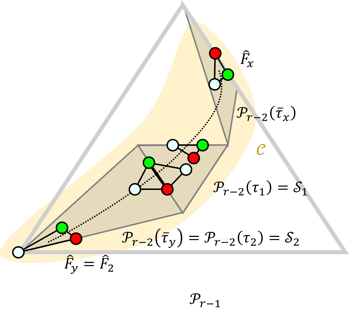
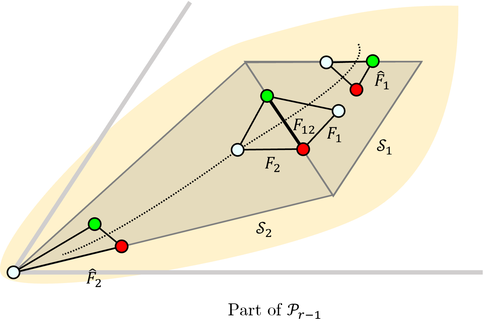
Figure 5: $P_{r-1}$

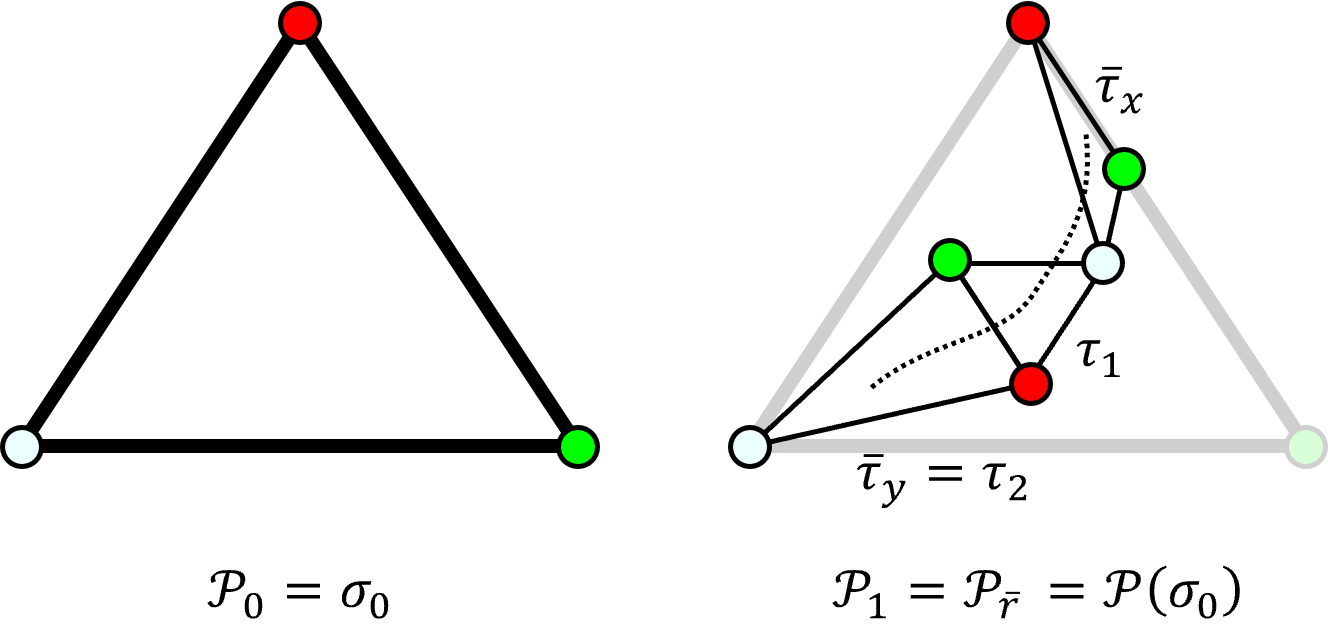
Figure 6: $\mathcal{P}_{0}$ and $P_{1}$

Since $\hat{F}_{x}$ and $\hat{F}_{y}$ are connected in $\mathcal{C}\subseteq\mathcal{P}_{r-1}$, $\overline{\tau}_{x}$ and $\overline{\tau}_{y}$ must be connected via one or more paths of adjacent facets in $\mathcal{P}_{1}$ as well. Consider an arbitrary, fixed path connecting the proper border facets $\hat{F}_{x}$ and $\hat{F}_{y}$ in $\mathcal{P}_{r-1}$, and its unique corresponding path connecting $\overline{\tau}_{x}$ and $\overline{\tau}_{y}$ in $\mathcal{P}_{1}$. Let $\tau_{1}$ and $\tau_{2}$ be any two adjacent facets on the path in $\mathcal{P}_{1}$, and $\tau_{12}=\tau_{1}\cap\tau_{2}\neq\emptyset$. In $\mathcal{P}_{r-1}$, the facets $\tau_{1}$ and $\tau_{2}$ induce connected subcomplexes $\mathcal{S}_{1}=\mathcal{P}^{r-2}(\tau_{1})$ and $\mathcal{S}_{2}=\mathcal{P}^{r-2}(\tau_{2})$ with a non-empty intersection $\mathcal{S}_{1}\cap\mathcal{S}_{2}\neq\emptyset$. The path from $\hat{F}_{x}$ to $\hat{F}_{y}$ in $\mathcal{P}_{r-1}$ must enter $\mathcal{S}_{1}$ at some facet $\hat{F}_{1}$ and exit $\mathcal{S}_{2}$ at some facet $\hat{F}_{2}$, i.e., there is a path connecting $\hat{F}_{x}$ to $\hat{F}_{1}$ and a path connecting $\hat{F}_{y}$ to $\hat{F}_{2}$, and cross the border between $\mathcal{S}_{1}$ and $\mathcal{S}_{2}$ via adjacent facets $F_{1}\in\mathcal{S}_{1}\subseteq\mathcal{P}_{r-1}$ and $F_{2}\in\mathcal{S}_{2}\subseteq\mathcal{P}_{r-1}$ with $\emptyset\neq F_{12}=F_{1}\cap F_{2}\in\mathcal{S}_{1}\cap\mathcal{S}_{2}$. Note that $F_{12}$, as the intersection of two facets in the protocol complex $\mathcal{P}_{r-1}$, is of course a face.

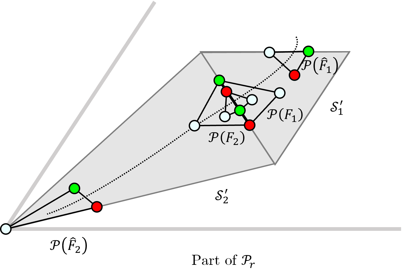
Figure 7: Part of $\mathcal{P}_{r}$

Now consider the outcome of applying $\mathcal{P}$ again to all the facets in $\mathcal{P}_{r-1}$, which of course gives $\mathcal{P}_{r}$ (see Fig. 7). In particular, this results in the subcomplexes $\mathcal{S}_{1}^{\prime}=\mathcal{P}\bigl{(}\mathcal{P}^{r-2}(\tau_{1})\bigr{)}=\mathcal{P}^{r-1}(\tau_{1})$ and analogously $\mathcal{S}_{2}^{\prime}=\mathcal{P}^{r-1}(\tau_{2})$, which may or may not have a non-empty intersection. We will be interested in the part of this possible intersection created by the application of $\mathcal{P}$ to $F_{1}$ and $F_{2}$, i.e., in $\mathcal{P}(F_{1})\cap\mathcal{P}(F_{2})\subseteq\mathcal{S}_{1}^{\prime}\cap\mathcal{S}_{2}^{\prime}$. Note that both $\mathcal{S}_{1}^{\prime}$ and $\mathcal{S}_{2}^{\prime}$ are isomorphic to $\mathcal{P}_{r-1}$. Clearly, the application of $\mathcal{P}$ to the facets $F_{1},F_{2}\in\mathcal{P}_{r-1}$ typically creates many pairs of intersecting border facets $F_{1}^{\prime}\in\mathcal{P}(F_{1})\subseteq\mathcal{S}_{1}^{\prime}\subseteq\mathcal{P}_{r}$ and $F_{2}^{\prime}\in\mathcal{P}(F_{2})\subseteq\mathcal{S}_{2}^{\prime}\subseteq\mathcal{P}_{r}$, such that each pair shares some non-empty face $\emptyset\neq F_{12}^{\prime}=F_{1}^{\prime}\cap F_{2}^{\prime}\subseteq\mathcal{S}_{1}^{\prime}\cap\mathcal{S}_{2}^{\prime}$. The shared faces $F_{12}^{\prime}$ together form the subcomplex $FC_{12}^{\prime}\subseteq\mathcal{P}(F_{1})\cap\mathcal{P}(F_{2})$ (see Fig. 8, left part, for two different examples).

 

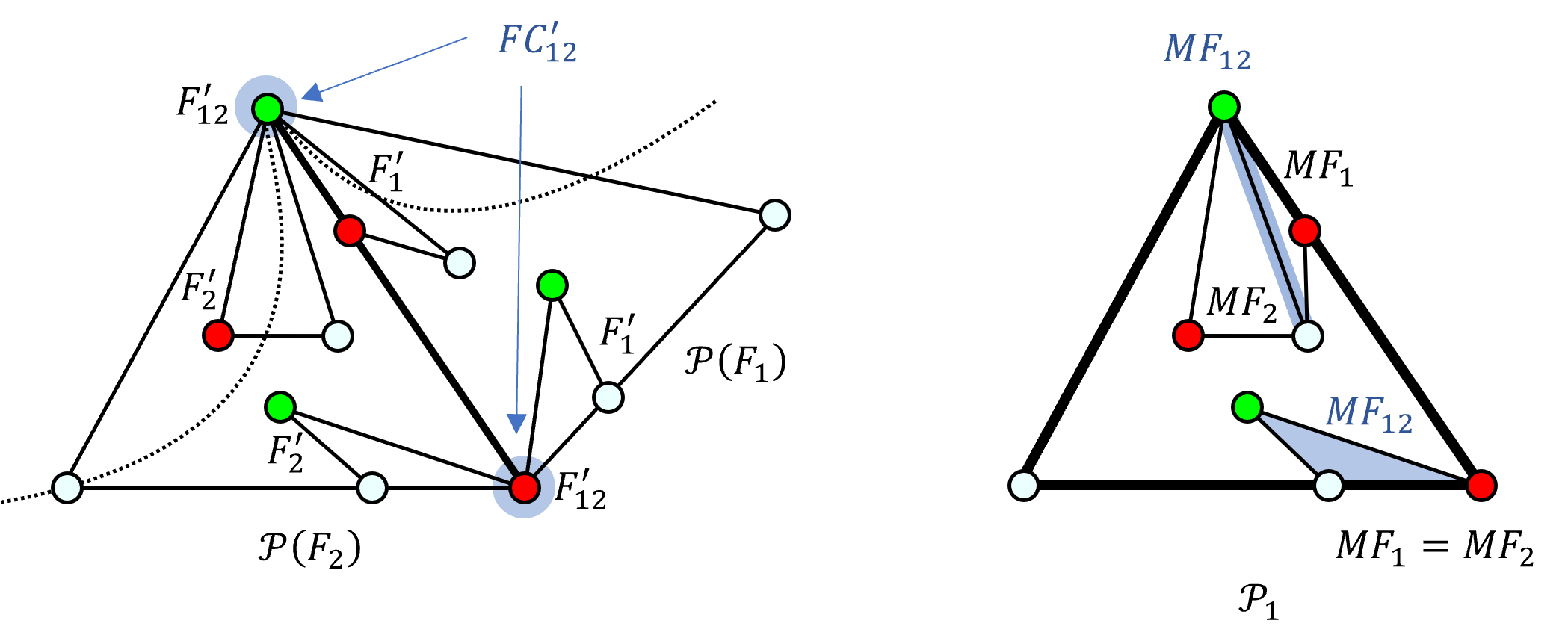
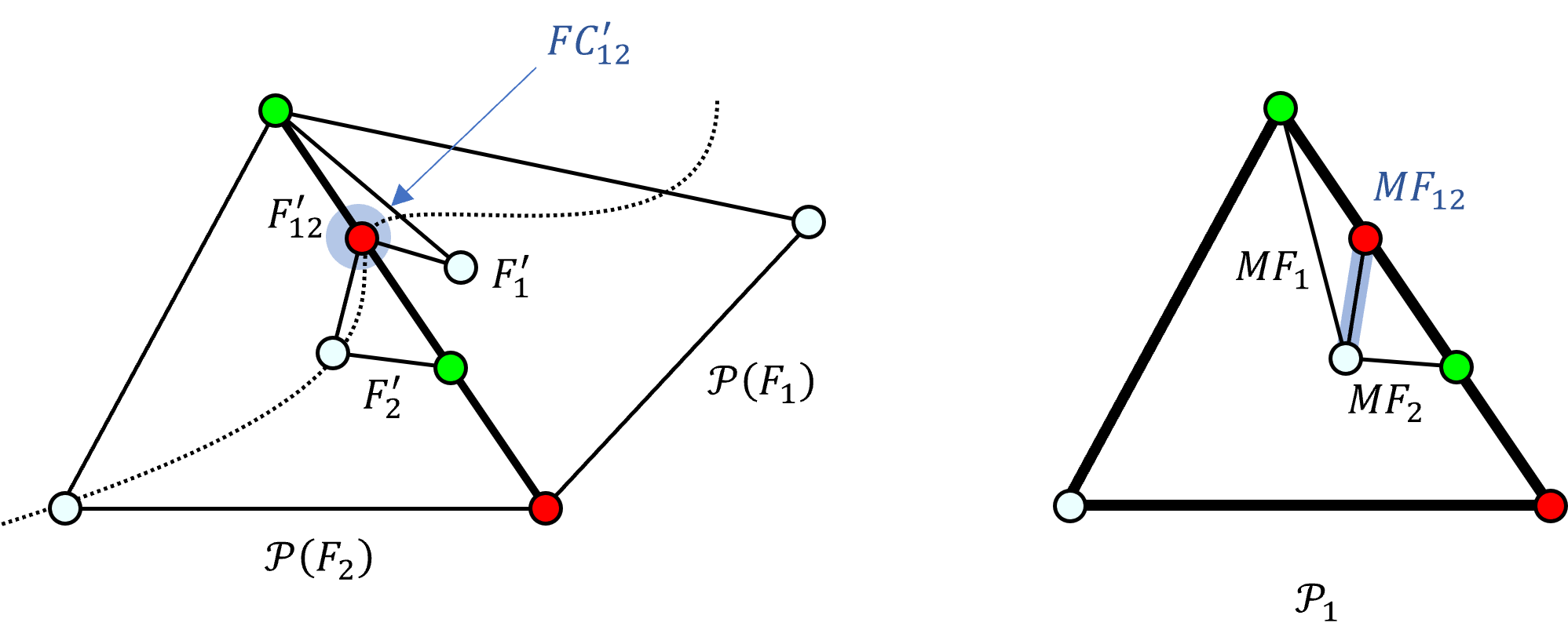
Figure 8: The subcomplex $FC_{12}^{\prime}\subseteq\mathcal{P}(F_{1})\cap\mathcal{P}(F_{2})$ in $\mathcal{P}_{r}$ and the corresponding subcomplex $MF_{12}$ in $\mathcal{P}_{1}$. Case $(1)$ top and Case $(2)$ bottom.

Any such $F_{12}^{\prime}$ is not completely arbitrary, though: First of all, since $FC_{12}^{\prime}\subseteq\mathcal{P}(F_{1})\cap\mathcal{P}(F_{2})$ implies that its colors can only be drawn from $\chi(F_{12})$ due to boundary consistency, we have

$$\chi(F_{12}^{\prime})\subseteq\chi(FC_{12}^{\prime})\subseteq\chi(F_{12}).$$ (17)

Moreover, every pair of properly intersecting facets $F_{1}^{\prime}$ and $F_{2}^{\prime}$ is actually created by two unique matching border facets $MF_{1},MF_{2}\in\mathcal{P}_{1}$: the adjacent facets $F_{1}^{\prime}\in\mathcal{P}(F_{1})$ and $F_{2}^{\prime}\in\mathcal{P}(F_{2})$ are isomorphic to some intersecting border facets $MF_{1}\in\mathcal{P}_{1}$ and $MF_{2}\in\mathcal{P}_{1}$, respectively, which match at the boundary (see Fig. 8, right part). This actually leaves only two possibilities for their intersection $MF_{12}=MF_{1}\cap MF_{2}\neq\emptyset$:

1. $MF_{1}$ and $MF_{2}$ are proper border facets with the same root component $R(MF_{1})=R(MF_{2})\in MF_{12}$ (possibly $MF_{12}\setminus R(MF_{1})\neq\emptyset$, though). Two instances are shown in the top part of Fig. 8.

2. $MF_{1}$ and $MF_{2}$ are proper border facets with different root components, or improper border facets, with $R(MF_{1})\cup R(MF_{2})\not\subseteq MF_{12}$ (taken as a complex). An instance is shown in the bottom part of Fig. 8.

Note that these are all possibilities, since our single-rootedness assumption rules out $R(MF_{1})\cup R(MF_{2})\subseteq MF_{12}$: After all, every $v\in R(MF_{1})\setminus R(MF_{2})\neq\emptyset$ (w.l.o.g.) would need to have an outgoing path to every vertex in $R(MF_{2})$, which is not allowed for the root component $R(MF_{2})$ by Definition 18. Keep in mind, for case (2) below, that every vertex in $MF_{12}$ must have an incoming path from every member of $R(MF_{1})$ in $MF_{1}$ and from every member of $R(MF_{2})$ in $MF_{2}$.

Now, given any pair of facets $F_{1}^{\prime}$ and $F_{2}^{\prime}$, we will consider conditions ensuring the lifting/breaking of paths that run over their intersection $F_{12}^{\prime}$. Not surprisingly, we will need to distinguish the two cases (1) and (2) introduced above. To support the detailed description of the different situations that can happen here, we recall the path in $\mathcal{C}\subseteq\mathcal{P}_{r-1}$ that forms our starting point (Fig. 5): It starts out from the proper border facet $\hat{F}_{x}$ and leads to $\hat{F}_{1}$, where it enters the subcomplex $\mathcal{S}_{1}=\mathcal{P}^{r-2}(\tau_{1})$. Within $\mathcal{S}_{1}$, the path continues to $F_{1}$. The latter has a non-empty intersection $F_{12}$ with $F_{2}$, which belongs to the subcomplex $\mathcal{S}_{2}=\mathcal{P}^{r-2}(\tau_{2})$. The path continues within $\mathcal{S}_{2}$ and exits it at $\hat{F}_{2}$, from where it finally leads to the proper border facet $\hat{F}_{y}$.

1. If $F_{12}^{\prime}=\emptyset$, i.e., the border facets $F_{1}^{\prime}$ and $F_{2}^{\prime}$ do not intersect at all, there obviously cannot be any path in $\mathcal{P}_{r}$ that connects $\hat{F}_{1}^{\prime}$ and $\hat{F}_{2}^{\prime}$ via $F_{12}^{\prime}$.

2. If $F_{12}^{\prime}\neq\emptyset$ is caused by proper border facets $F_{1}^{\prime}$ and $F_{2}^{\prime}\in\mathcal{P}_{r}$ with the same border root component $R(F_{1}^{\prime})=R(F_{2}^{\prime})$, then both $F_{1}^{\prime}\in\mathcal{P}_{r}$ and $MF_{1}\in\mathcal{P}_{1}$ are isomorphic to some proper border facet $BF_{1}\in\mathcal{P}_{r-1}$; analogously, $F_{2}^{\prime}\in\mathcal{P}_{r}$ and $MF_{2}\in\mathcal{P}_{1}$ are both isomorphic to some proper border facet $BF_{2}\in\mathcal{P}_{r-1}$. This holds since $\mathcal{S}_{1}^{\prime}=\mathcal{P}^{r-1}(\tau_{1})$ and $\mathcal{S}_{2}^{\prime}=\mathcal{P}^{r-1}(\tau_{2})$ are both isomorphic to $\mathcal{P}_{r-1}$. Note carefully, though, that $BF_{12}=BF_{1}\cap BF_{2}$ is isomorphic to $F_{12}^{\prime}$ (but not necessarily to $MF_{12}$, as can be seen in the top of Fig. 8), so $\chi(R(BF_{1}))=\chi(R(BF_{2}))\subseteq\chi(BF_{12})\subseteq\chi(F_{12}^{\prime})\subseteq\chi(F_{12})$ by Eq. 17. Note that Definition 20 immediately implies $B(BF_{1})=B(BF_{2})\subseteq BF_{12}$ for the respective border components as well.

   Depending on $BF_{1}$ and $BF_{2}$ (actually, depending on $BF_{12}$ and, ultimately, on $R(BF_{1})=R(BF_{2})$, which we will say to protect $F_{12}$), all paths running over $R(F_{1}^{\prime})=R(F_{2}^{\prime})$ will either (a) be lifted or else (b) break:

   1. We say that $R(BF_{1})=R(BF_{2})$ successfully protects $F_{12}$ (see Fig. 9) if $BF_{12}\in\mathcal{C}$, i.e., if both $BF_{1}$ and $BF_{2}$ are within the same connected component $\mathcal{C}$ as $F_{1}$ and $F_{2}$ (which also implies that there are paths in $\mathcal{C}$ connecting $\hat{F}_{1}$ to $BF_{1}$ and $\hat{F}_{2}$ to $BF_{2}$). In this case, there is a lifted path in $\mathcal{P}_{r}$ connecting some border facets $\hat{F}_{1}^{\prime}\in\mathcal{P}(\hat{F}_{1})$ and $\hat{F}_{2}^{\prime}\in\mathcal{P}(\hat{F}_{2})$ via $BF_{12}$, carried by the one in $\mathcal{P}_{r-1}$ that connected the proper border facets $\hat{F}_{1}$ and $\hat{F}_{2}$ via $F_{12}$: It exists, since both $\mathcal{S}_{1}^{\prime}=\mathcal{P}^{r-1}(\tau_{1})$ and $\mathcal{S}_{2}^{\prime}=\mathcal{P}^{r-1}(\tau_{2})$ are isomorphic to $\mathcal{P}_{r-1}$. By applying $\mathcal{P}$ to all remaining facets on the path that connected $\hat{F}_{x}$ and $\hat{F}_{y}$ in $\mathcal{P}_{r-1}$ as well, a path in $\mathcal{P}_{r}$ may be created that connects some incompatible proper border facets $\hat{F}_{x}^{\prime},\hat{F}_{y}^{\prime}\in\mathcal{P}_{r}$; of course, this requires a successful lifting everywhere along the original path, not just at the intersection between $F_{1}$ and $F_{2}$.

   2. We say that $R(BF_{1})=R(BF_{2})$ unsuccessfully protects $F_{12}$ if $BF_{12}\not\in\mathcal{C}$. In this case, there cannot be a path connecting the border facets $\hat{F}_{1}^{\prime}$ and $\hat{F}_{2}^{\prime}$ in $\mathcal{P}_{r}$ running via $BF_{12}$, i.e., the connecting path in $\mathcal{P}_{r-1}$ cannot be lifted to $\mathcal{P}_{r}$ and thus breaks!

   

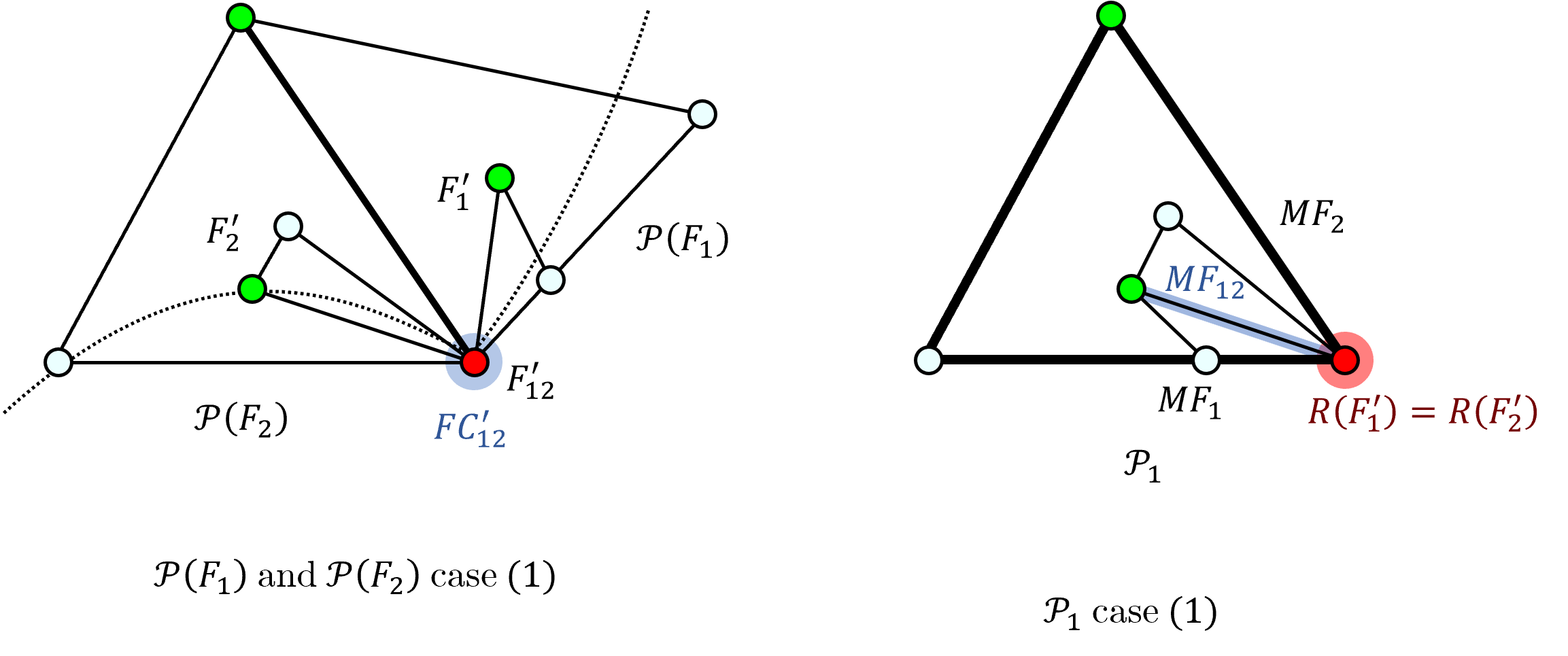
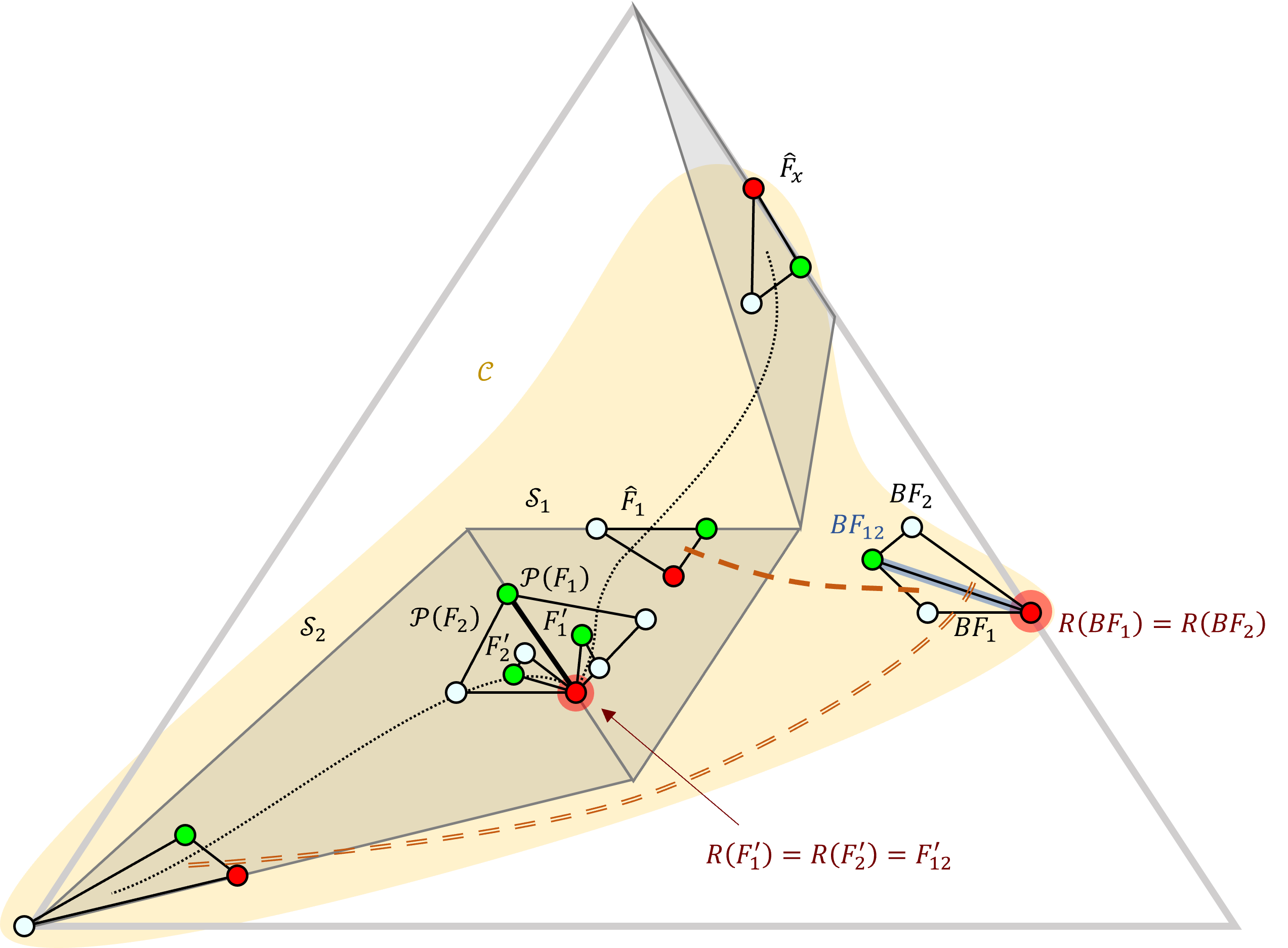
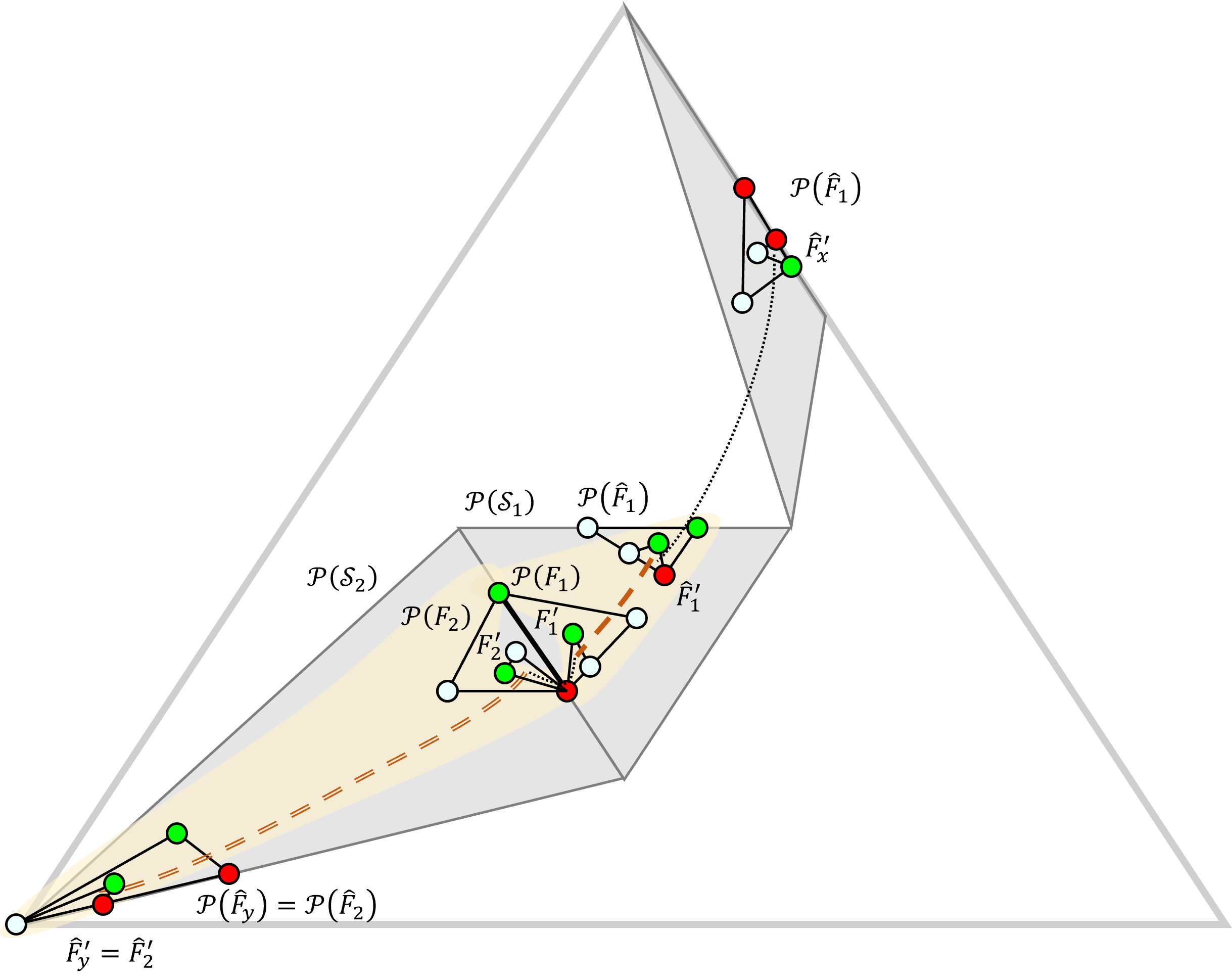
   $\mathcal{P}(F_{1})$ and $\mathcal{P}(F_{2})$ in $\mathcal{P}_{r}$, and the corresponding subcomplexes $MF_{1}$ and $MF_{2}$ in $\mathcal{P}_{1}$ $\mathcal{P}_{r-1}$ $\mathcal{P}_{r}$ with the images of $\mathcal{C}$ in $\mathcal{S}_{1}$ and $\mathcal{S}_{2}$ marked

   Figure 9: Lifting — Case 1(a)

3. If $F_{12}^{\prime}\neq\emptyset$ is not caused by proper border facets $F_{1}^{\prime}\in\mathcal{P}_{r}$ and $F_{2}^{\prime}\in\mathcal{P}_{r}$ with common border root components $R(F_{1}^{\prime})=R(F_{2}^{\prime})$, we know from (2) above that $R(MF_{1})\cup R(MF_{2})\not\subseteq MF_{12}$, i.e., at least one of the root components, say, $R(F_{1}^{\prime})$, has a vertex $v_{1}^{\prime}\in F_{1}^{\prime}$ outside $F_{12}^{\prime}$. Clearly, the corresponding vertex $v_{2}^{\prime}\in F_{2}^{\prime}$ with $\chi(v_{1}^{\prime})=\chi(v_{2}^{\prime})$ is also outside $F_{12}^{\prime}$ and hence different from $v_{1}^{\prime}$. Since there is a path from $v_{1}^{\prime}$ to every vertex in $F_{1}^{\prime}$, at least one member in the intersection $F_{12}$ will be gone in $F_{12}^{\prime}$, so

   $$|V(F_{12}^{\prime})|<|V(F_{12})|.$$ (18)

This completes the (exhaustive) list of cases that need to be considered w.r.t. a single pair of facets $F_{1}^{\prime}$ and $F_{2}^{\prime}$. Clearly, in order for a lifted path connecting $\hat{F}_{x}^{\prime}$ and $\hat{F}_{y}^{\prime}$ in $\mathcal{P}_{r}$ to break, it suffices that it breaks for just one pair of adjacent facets. On the other hand, for a given pair $F_{1},F_{2}\in\mathcal{P}_{r-1}$, many paths are potentially created simultaneously in $\mathcal{P}_{r}$, each corresponding to a possible selection of $F_{1}^{\prime}$ and $F_{2}^{\prime}$ and the particular intersection facet $F_{12}^{\prime}$, which all need to break eventually. Moreover, there are different paths in $\mathcal{P}_{r-1}$ connecting $\hat{F}_{x}$ and $\hat{F}_{y}$ via different pairs $F_{1},F_{2}$ that need to be considered. In LABEL:sec:terminationtime, we will show that there is even another subtle complication caused by case (1.b), the case where there is no lifted path in $\mathcal{P}_{r}$: It will turn out that “bypassing” may create a new path connecting some incompatible proper border facets in $\mathcal{P}_{r}$ when the path in $\mathcal{P}_{r-1}$ breaks; see LABEL:fig:multipath for an example.

Finally, for consensus to be solvable, no connected component $\mathcal{C}$ containing all border facets $\hat{F}_{1},\dots,\hat{F}_{k}\in\mathcal{C}$ with incompatible border components $\hat{B}_{1},\dots,\hat{B}_{k}$ may exist. In other words, there must be some $r$ such that none of the connected components of $\mathcal{P}_{r}$ contains facets with incompatible border components. If this is ensured, the processes in any facet $F\in C\subseteq\mathcal{P}_{r}$ can eventually decide on the initial value of a deterministically chosen process in $\bigcap_{F\in\mathcal{C},B(F)\neq\emptyset}\operatorname{\beta}(F)\neq\emptyset$. Note carefully, however, that this also requires that all connections between incompatible borders that are caused by facet borders different from the border component $B(F)$ have disappeared. Since this is solely a matter of case (2), Eq. 18 reveals that this must happen after at most $n-1$ additional rounds.

4.3 Characterizing consensus solvability via connected components

It is enlightening to view cases (0)–(2) introduced before w.r.t. the effect that they cause on the connected component $\mathcal{C}\subseteq\mathcal{P}_{r-1}$ that connects incompatible border facets: Reconsider the two adjacent facets $F_{1},F_{2}\in\mathcal{C}$ with intersection $F_{12}$, and assume, for clarity of the exposition, that $\mathcal{C}$ would fall apart if the path running over $F_{12}$ would break. We will now discuss what happens w.r.t. the connected component(s) in $\mathcal{P}_{r}$ when going to $F_{1}^{\prime}\in\mathcal{P}(F_{1})$ and $F_{2}^{\prime}\in\mathcal{P}(F_{2})$, under the assumption that $F_{12}^{\prime}$ is the only intersecting facet in $\mathcal{P}_{r}$, according to our three cases:

1. If $F_{12}^{\prime}=\emptyset$, then $\mathcal{P}_{r}$ would contain two separate connected components $\mathcal{C}_{1}^{\prime}$ and $\mathcal{C}_{2}^{\prime}$ with $F_{1}^{\prime}\in\mathcal{C}_{1}^{\prime}$ and $F_{2}^{\prime}\in\mathcal{C}_{2}^{\prime}$, i.e., the connected component(s) in $\mathcal{P}_{r}$ resulting from $\mathcal{C}$ are separated by what is generated from $F_{12}$, namely, $F_{12}^{\prime}=\emptyset$. A nice example is the (shaded) green center node in $\mathcal{P}_{2}^{RAS}$ of the RAS message adversary shown in Fig. 3.

2. If $F_{12}^{\prime}\neq\emptyset$ is caused by proper border facets $F_{1}^{\prime}\in\mathcal{P}_{r}$ and $F_{2}^{\prime}\in\mathcal{P}_{r}$ (isomorphic to $BF_{1}$ resp. $BF_{2}$) with the same border root component $R(F_{1}^{\prime})=R(F_{2}^{\prime})=F_{12}^{\prime}$ that successfully protects $F_{12}$, we have our two subcases:

   1. If $BF_{12}\in\mathcal{C}$, then $\mathcal{P}_{r}$ would contain a single connected component $\mathcal{C}^{\prime}$ (resulting from $\mathcal{C}$) that connects incompatible border facets. An instance of such a successful protection can be found in Fig. 10 of $\mathcal{P}_{2}^{iRAS}$ for the iRAS message adversary, where consensus is impossible. Note that just one communication graph has been added to RAS here, namely, the additional triangle that connects the bottom left white vertex to the central triangle in the 1-round uninterpreted complex $\mathcal{P}_{1}^{iRAS}$ in the top left part of Fig. 10. Consider the left border of the dash-dotted central triangle, for example, where two adjacent facets intersect in the common root $r\leftrightarrow g$. It results from the fact that the border root component $r\leftrightarrow g$ of the proper border facet on the right outermost border of the protocol complex $\mathcal{P}_{1}^{iRAS}$ protects the intersection $r\leftrightarrow g$ of the central facet and the facet left to it in $\mathcal{P}_{1}^{iRAS}$.

      Figure 10: Protocol complex for one round ($\mathcal{P}=\mathcal{P}_{1}^{iRAS}$, top) and two rounds ($\mathcal{P}_{2}^{iRAS}$, bottom) of the iRAS message adversary. The top right figure also shows the border root components of $\mathcal{P}$.

   2. If $BF_{12}\not\in\mathcal{C}$, then $\mathcal{P}_{r}$ would contain two connected components $\mathcal{C}_{1}^{\prime}$ and $\mathcal{C}_{2}^{\prime}$ with $F_{1}^{\prime}\in\mathcal{C}_{1}^{\prime}$ and $F_{2}^{\prime}\in\mathcal{C}_{2}^{\prime}$. Unlike in case (0), however, they are separated by a third connected component $\mathcal{C}_{12}^{\prime}$ that contains $F_{1}^{\prime}$ and $F_{2}^{\prime}$. It can be viewed as an “island” that develops around $F_{12}^{\prime}$. A nice example of such an unsuccessful protection is the connected component containing the red process in the center of Fig. 11 for $\mathcal{P}_{2}^{2C}$ for the two-chain message adversary, which now separates the single connected component containing this process in $\mathcal{P}_{1}^{2C}$.

      We note that the bypassing effect already mentioned (and discussed in detail in LABEL:sec:terminationtime) can also be easily explained via this view: It could happen that the “island” $C_{12}^{\prime}$ is such that it connects some other incompatible proper border facets in $\mathcal{P}_{r}$ (see LABEL:fig:multipath for an example). So whereas it successfully separates $\mathcal{C}_{1}^{\prime}$ and $\mathcal{C}_{2}^{\prime}$, it creates a new path that prohibits the termination of consensus in round $r$.

3. If $F_{12}^{\prime}\neq\emptyset$ is not caused by a proper border facet $F_{1}^{\prime}\in\mathcal{P}_{r}$ and $F_{2}^{\prime}\in\mathcal{P}_{r}$ with common border root component $R(F_{1}^{\prime})=R(F_{2}^{\prime})=F_{12}^{\prime}$, $\mathcal{P}_{r}$ would contain a single connected component $\mathcal{C}^{\prime}$ (resulting from $\mathcal{C}$) that still connects incompatible border facets.

4.4 Examples

An example of an unsuccessful protection (a breaking path, case (1.b)) can be found in the 1-round uninterpreted complex $\mathcal{P}_{1}^{RAS}$ for the RAS message adversary in the top-right part of Fig. 3, where the facets $\hat{F}_{x}$ and $\hat{F}_{y}$ containing the border root components $\hat{R}_{x}$ (the single white vertex in the bottom-left corner) and $\hat{R}_{y}$ (the bidirectionally connected red and green vertices on the right border) are connected by a path that runs over the bottom leftmost triangle $F_{1}=\hat{F}_{x}$ and the central triangle $F_{2}$, in a joint connected component $\mathcal{C}\subseteq\mathcal{P}_{1}^{RAS}$. Note that $F_{1}$ and $F_{2}$ intersect in the single green central vertex $F_{12}=F_{1}\cap F_{2}=\{g\}$, and that there is no facet with a border (root) component consisting only of the green vertex in $\mathcal{P}_{1}$ and hence in $\mathcal{C}$. Consequently, it follows that $\mathcal{P}_{2}^{RAS}$ cannot contain a corresponding path connecting $\hat{F}_{x}^{\prime}$ with border root component $\hat{R}_{x}^{\prime}$ (the single white vertex in the bottom-left corner in the bottom part of Fig. 3) and $\hat{R}_{y}^{\prime}$ (the bidirectionally connected red and green vertices on the right outer border) running over the faded central vertex $F_{12}^{\prime}=\{g\}$, as is confirmed by our figure.

For an example of a successful protection (a non-breaking path, case (1.a)), consider the path connecting the border facets $\hat{F}_{x}$ and $\hat{F}_{z}$ containing the border root components $\hat{R}_{x}$ (the single white vertex in the bottom-left corner) and $\hat{R}_{z}$ (the bidirectionally connected red and white vertices on the left border) in the top-right part of Fig. 3. This path only consists of the bottom leftmost triangle $F_{1}=\hat{F}_{x}$ and the triangle $F_{2}=\hat{F}_{z}$ in a joint connected component $\mathcal{C}\subseteq\mathcal{P}_{1}^{RAS}$. Note that $F_{1}$ and $F_{2}$ intersect in a red-green edge $F_{12}=F_{1}\cap F_{2}=\{r\to g\}$ here, and that there is the border facet $\hat{F}_{y}\in\mathcal{C}$ with a border root component $\hat{R}_{y}=\{g\leftrightarrow r\}$ on the rightmost outer border. According to our considerations above, $\mathcal{P}_{2}^{RAS}$ contains a corresponding path connecting $\hat{F}_{x}^{\prime}$ with border root component $\hat{R}_{x}^{\prime}$ (the single white vertex in the bottom-left corner in the bottom part of Fig. 3) and the border facet $\hat{F}_{z}^{\prime}$ with border root component $\hat{R}_{z}^{\prime}$ (the bidirectionally connected red and white vertices on the leftmost outer border) running via $F_{12}^{\prime}=\{g\leftrightarrow r\}$, as is confirmed by our figure.

To further illustrate the issue of successful/unsuccessful protection, consider the modified RAS message adversary iRAS depicted in Fig. 10, where consensus is impossible. The border facets $\hat{F}_{w}$ (the additional triangle) resp. $\hat{F}_{y}$ containing the border root component $\hat{R}_{w}$ (the single white vertex in the bottom-left corner) resp. $\hat{R}_{y}$ (the bidirectionally connected red and green vertices on the right border) are connected by a path that runs over the central bidirectional red-green edge $F_{12}=F_{1}\cap F_{2}=\{g\leftrightarrow r\}$ in $\mathcal{C}$ here. In sharp contrast to RAS, the border facet $\hat{F}_{y}$ with the border root component $\hat{R}_{y}=\{g\leftrightarrow r\}$ on the right outer border is now also in $\mathcal{C}$, however. Consequently, $\mathcal{P}_{2}^{RAS}$ contains a corresponding path connecting $\hat{F}_{w}^{\prime}$ with border root component $\hat{R}_{w}^{\prime}$ (the single white vertex in the bottom-left corner in the bottom part of Fig. 10) and $\hat{F}_{y}^{\prime}$ with border root component $\hat{R}_{y}^{\prime}$ (the bidirectionally connected red and green vertices on the right outer border) running via $F_{12}^{\prime}=\{g\leftrightarrow r\}$, as is confirmed by our figure. Note that this situation recurs also in all further rounds, making consensus impossible.

To illustrate the issue of delayed path breaking (case (2)), consider another message adversary, called the 2-chain message adversary (2C), shown for $n=4$ processes in Fig. 11 (top part). It consists of three graphs, a chain $G_{1}=y\to g\to w\to r$, another chain $G_{2}=g\to y\to w\to r$, and a star $G_{3}=r\to\{y,w,g\}$. In $\mathcal{P}_{1}$, the facets $F_{1}$ and $F_{2}$, corresponding to $G_{1}$ and $G_{2}$, respectively, are connected by a path running over the intersection $F_{12}=\{r\}$ in a joint connected component $\mathcal{C}$. There is also a border root component $R=\{r\}$ in the facet $F_{3}$ resulting from $G_{3}$, which, however, lies in a different connected component $\mathcal{C}^{\prime}\neq\mathcal{C}$ in $\mathcal{P}$. According to our considerations (case (1.b), the path (potentially) connecting $F_{1}^{\prime}$ (the border facet representing $G_{1}$ both in round 1 and 2) and $F_{2}^{\prime}$ (the border facet representing $G_{2}$ both in round 1 and 2) via $F_{12}^{\prime}=\{r\}$ in $\mathcal{P}_{2}^{2C}$ breaks: As is apparent from the bottom part of Fig. 11, there is no single red vertex shared by these two facets.

If one adds another process $p$ (pink) to 2C for $n=5$, denoted by the message adversary 2C+, such that $G_{1}=y\to g\to w\to p\to r$, $G_{2}=g\to y\to w\to p\to r$, and $G_{3}=r\to\{y,w,g,p\}$, then $F_{12}=\{p\to r\}$ is in $\mathcal{P}_{1}^{2C+}$. Now there is a path in $\mathcal{P}_{2}^{2C+}$ connecting $F_{1}^{\prime}$ (the border facet representing $G_{1}$ both in round 1 and 2) and $F_{2}^{\prime}$ (the border facet representing $G_{2}$ both in round 1 and 2) running via $F_{12}^{\prime}=F_{1}^{\prime}\cap F_{2}^{\prime}=\{r\}$: Whereas the pink vertex has learned in round 2 where it belongs to, i.e., either $F_{1}^{\prime}$ and $F_{2}^{\prime}$, from the respective root component, this is not (yet) the case for the red vertex. However, whereas the corresponding path did not break in $\mathcal{P}_{2}^{2C+}$, it will finally break in $\mathcal{P}_{3}^{2C}$ since the red vertex will also learn where it belongs to.

Figure 11: Protocol complex for one round ($\mathcal{P}=\mathcal{P}_{1}^{2C}$, top) and two rounds ($\mathcal{P}_{2}^{2C}$, bottom) of the two-chain message adversary for $n=4$ processes. The top right figure also shows the border root components of $\mathcal{P}$.

4.5 A decision procedure for consensus solvability

Revisiting the different cases (0)–(2) that can occur w.r.t. lifting/breaking a path connecting incompatible border facets in $\mathcal{P}_{r-1}$ to $\mathcal{P}_{r}$, it is apparent that the only case that might lead to a path that never breaks, i.e., in no round $r\geq 1$, is case (1.a): In case (0) and (1.b), there cannot be a lifted path running via $F_{12}^{\prime}$ in $\mathcal{P}_{r}$, i.e., the path in $\mathcal{P}_{r-1}$ breaks immediately. In case (2), it follows from Eq. 18 that this type of lifting could re-occur in at most $n-2$ consecutive rounds after a path running over $F_{12}$ is lifted to a path running over $F_{12}^{\prime}$ in $\mathcal{P}_{r}$ for the first time. Since these are all possibilities, after the “exhaustion” of case (2), $F_{12}^{\prime}=\emptyset$ and hence case (0) necessarily applies.

In order to decide whether consensus is solvable for a given message adversary $\mathbf{D}^{\omega}$ at all, it hence suffices to keep track of case (1.a) over rounds $1,2,\dots$. If one finds that case (1.a) does not occur for any path in $\mathcal{P}_{r-1}$ for some $r$, there is no need for iterating further. On the other hand, if one finds that case (1.a) re-occurs for some path forever, consensus is impossible. Since the facets $BF_{1}$ and $BF_{2}$, where the common root component $R(BF_{1})=R(BF_{2})$ successfully protects $F_{12}$ in case (1.a), leads to $\chi(F_{12}^{\prime})\subseteq\chi(F_{12})$ according to Eq. 17, the infinite re-occurence of case (1.a) for some path implies that there is some round $r_{0}$ such that $\chi(F_{12}^{\prime})=\chi(F_{12})=I\subset\Pi$ for all $r\geq r_{0}$. If this holds true, then case (1.a) must also re-occur perpetually in the lifted paths obtained by using the same $BF_{1}$ and $BF_{2}$ with $\chi(BF_{12})=I$ in all rounds $r\geq r_{0}$.

For keeping track of possibly infinite re-occurrences of case (1.a), it is hence sufficient to determine, for every pair of facets $MF_{1}\in\mathcal{P}_{1}$ and $MF_{2}\in\mathcal{P}_{1}$, $MF_{2}\neq MF_{1}$, intersecting in $MF_{12}\neq\emptyset$, the set of proper border facets $MF^{1},\dots,MF^{\ell}\in\mathcal{P}_{1}$ with border root components $R^{j}=R(MF^{j})$ satisfying $\chi(R^{j})\subseteq\chi(MF_{12})$ for all $1\leq j\leq\ell$. Clearly, every choice of $MF^{j}$, $MF^{k}$ is a possible candidate for the isomorphic re-occurring protecting facets $BF_{1}=BF^{j}$ and $BF_{2}=BF^{k}$ for case (1.a) in some $\mathcal{P}_{r-1}$, provided (i) $R(MF^{j})=R(MF^{k})$ and (ii) both $BF^{j}$ and $BF^{k}$ are in the connected component $\mathcal{C}\subseteq\mathcal{P}_{r-1}$ containing $F_{1}$ and $F_{2}$. If (ii) does not hold, one can safely drop $MF^{j}$, $MF^{k}$ from the set of candidates for infinitely re-occurring protecting facets in all subsequent rounds.

This can be operationalized in an elegant and efficient decision procedure by using an appropriately labeled and weighted version of the facets’ nerve graph $\mathcal{N}$ of the 1-round uninterpreted complex $\mathcal{P}_{1}$. It is a topological version of the combinatorial decision procedure given in [WPRSS23:ITCS, Alg. 1] that works as follows: Every facet in $\mathcal{P}_{1}$ is a node $F$ in $\mathcal{N}$ and labeled by $w(F)=R(F)$, its root component in $\mathcal{P}_{1}$. Two nodes $F^{1},F^{2}$ in $\mathcal{N}$ are joined by an (undirected) edge $(F^{1},F^{2})$, if they intersect in a simplex $\emptyset\neq F^{12}=F^{1}\cap F^{2}$ in $\mathcal{P}_{1}$. The edge is labeled by $w((F^{1},F^{2}))=\{R^{1},\dots,R^{\ell}\}$ (possibly empty), which is the maximal set of (necessarily: border) root components that satisfy the property $\chi(F^{12})\supseteq\chi(R^{i})$. Recall that the member sets of different border root components may satisfy $\chi(R^{i})\cap\chi(R^{j})\neq\emptyset$ and even $\chi(R^{i})=\chi(R^{j})$, albeit $R^{i}\cap R^{j}\neq\emptyset$ when taken as faces is impossible.

The procedure for deciding on consensus solvability proceeds in iterations, starting from $\mathcal{N}_{0}=\mathcal{N}$, and defining $\mathcal{N}_{i+1}$ from $\mathcal{N}_{i}$ as follows. Let $V(\mathcal{N}_{i+1}):=V(\mathcal{N}_{i})$ with the same node labels $w(F)$, initialize $E(\mathcal{N}_{i+1})$ to be the empty set, and add to it each edge $(F^{1},F^{2})\in E(\mathcal{N}_{i})$ with a label $w_{i+1}((F^{1},F^{2}))$ defined next, but only if this label is not empty. For a potential edge $(F^{1},F^{2})\in E(\mathcal{N}_{i})$, set $R\in w_{i+1}((F^{1},F^{2}))$ if the (unique) connected component $C_{i}^{j}$ of $\mathcal{N}_{i}$ with $(F^{1},F^{2})\in E(\mathcal{C}_{i}^{j})$ contains some $F^{\prime}\in V(\mathcal{C}_{i}^{j})$ with $w(F^{\prime})=R\in w_{i}((F^{1},F^{2}))$. The construction stops when either (i) none of the connected components of $\mathcal{N}_{i}$ contains nodes representing facets with incompatible root components (consensus is solvable), or else (ii) if $\mathcal{N}_{i+1}=\mathcal{N}_{i}$ but there is at least one connected component containing nodes representing facets with incompatible root components (consensus is impossible).

For example, Fig. 12 shows the labeling of the facets with their root components for the RAS message adversary, where consensus can be solved. The sequence of nerve graphs $\mathcal{N}$, $\mathcal{N}_{0}$ and $\mathcal{N}_{1}$ is illustrated in Fig. 13. On the other hand, Fig. 14 and LABEL:fig:iRASnerve show the same for the iRAS message adversary, where consensus cannot be solved.

Figure 12: Results of labeling the faces of the 1-layer protocol complex $\mathcal{P}_{1}$ of the RAS message adversary (left) by their root component (right).

Figure 13: Construction of the initial nerve graph $\mathcal{N}_{0}$ of the 1-layer protocol complex $\mathcal{P}_{1}$ of the RAS message adversary: After replacing the facets by their corresponding nodes (colored by their root component) and labeling all the edges (left), nerve graph $\mathcal{N}_{0}$ obtained by removing edges without a protecting root component (middle), nerve graph $\mathcal{N}_{1}$ (right). Note that $\mathcal{N}_{1}$ already reveals that consensus is solvable.

Figure 14: Results of labeling the faces of the 1-layer protocol complex $\mathcal{P}_{1}$ of the iRAS message adversary (left) by their root component (right).