Extended atomic data for oxygen abundance analyses

As the most abundant element in the universe after hydrogen and helium, oxygen plays a key role in planetary, stellar, and galactic astrophysics. Its abundance is especially influential on stellar structure and evolution, and as the dominant opacity contributor at the base of the Sun’s convection zone it is central to the discussion around the solar modelling problem. However, abundance analyses require complete and reliable sets of atomic data. We present extensive atomic data for O I, by using the multiconfiguration Dirac–Hartree–Fock and relativistic configuration interaction methods. Lifetimes and transition probabilities for radiative electric dipole transitions are given and compared with results from previous calculations and available measurements. The accuracy of the computed transition rates is evaluated by the differences between the transition rates in Babushkin and Coulomb gauges, as well as by a cancellation factor analysis. Out of the 989 computed transitions in this work, 205 are assigned to the accuracy classes AA-B, that is, with uncertainties less than 10%, following the criteria defined by the National Institute of Standards and Technology Atomic Spectra Database. We discuss the influence of the new log($gf$) values on the solar oxygen abundance and ultimately advocate $\log\epsilon_{\mathrm{O}}=8.70\pm 0.04$.

1 Introduction

Oxygen is the most abundant metal in the universe. It is a key tracer of the evolution of galaxies (for example, Romano, 2022), as well as of the formation and characterisation of exoplanets (for example, Kolecki & Wang, 2022). In the interiors of stars, oxygen is a major source of opacity; for example in the Sun it is the dominant source near the base of the convection zone (for example Mondet et al., 2015). This makes the solar oxygen abundance critically important for resolving the solar modelling problem, which describes a significant discrepancy between theoretical predictions of the solar interior structure inferred from helioseismic inversions compared to standard solar models (for example, Vinyoles et al., 2017; Christensen-Dalsgaard, 2021).

The abundance of oxygen in stellar atmospheres can be determined from analyses of stellar spectra. In AFGK-type stars, one of the most commonly used oxygen abundance diagnostics is the high-excitation O i 777 nm triplet (for example Nissen et al., 2014; Buder et al., 2021). Other permitted atomic features are sometimes used as well: most commonly the O i 615.8 nm (Korotin et al., 2014; Delgado Mena et al., 2021); and for the Sun also the O i 844.7 nm and 926.9 nm multiplets (Asplund et al., 2004, 2021; Caffau et al., 2008). These are often complemented by low-excitation forbidden features, usually the [O i] 630.0 nm (Bertran de Lis et al., 2015; Franchini et al., 2021), and for the Sun also the [O i] 557.7 nm and 636.3 nm lines (Allende Prieto et al., 2001; Meléndez & Asplund, 2008), although at least in the solar spectrum these are significantly blended. Oxygen abundances can also be inferred from molecular diagnostics, in particular OH lines in the UV and infrared (Israelian et al., 1998; Boesgaard et al., 1999; Meléndez & Barbuy, 2002), although such lines are typically more sensitive to the effects of stellar convection (for example Asplund & García Pérez, 2001; Amarsi et al., 2021).

The accuracy of abundance determinations is critically dependent on reliability of the radiative transition probabilities. Moreover, if the assumption of local thermodynamic equilibrium (LTE) is to be relaxed, as is necessary for the O i 777 nm triplet and other high-excitation permitted atomic oxygen lines (for example, Steffen et al., 2015; Amarsi et al., 2016), a large set of reliable transition probabilities are needed to accurately determine the statistical equilibrium.

The vast majority of transition probabilities for atomic oxygen come from theoretical calculations. The transition probabilities and oscillator strengths of O i presented in the Atomic Spectra Database of the National Institute of Standards and Technology (NIST-ASD; see Kramida et al. 2022) were compiled by Wiese et al. (1996) based on the theoretical calculations from Hibbert et al. (1991), Butler & Zeippen (1991), and Biemont & Zeippen (1992). Hibbert et al. (1991) computed the oscillator strengths for a large number of allowed transitions connecting the $n$ $\leq$ 4 triplet and quintet states of neutral oxygen, using the CIV3 code. Butler & Zeippen (1991) performed the calculations of oscillator strengths for allowed transitions in O i, in the framework of the international Opacity Project. Using the atomic structure computer program SUPERSTRUCTURE, Biemont & Zeippen (1992) calculated the oscillator strengths for 2$p$-3$s$ and 3$s$-3$p$ spin-allowed or spin-forbidden transitions of astrophysical interest.

There are also a number of other calculations available for O i. The complete lists of published papers can be retrieved from the NIST Atomic Transition Probability Bibliographic database (Kramida, 2023). Tachiev & Froese Fischer (2002) performed multi-configurational Hartree-Fock (MCHF) calculations including Breit-Pauli effects in subsequent configuration-interaction calculations and determined lifetimes and transitions rates for all fine-structure levels up to ${2p^{3}3d}$ of the oxygen-like sequence (elements with atomic number $Z$ = 8-20). Zheng & Wang (2002) calculated the atomic data, including the radiative lifetimes, transition probabilities, and oscillator strengths in O i, by employing the weakest bound electron potential model theory. Using the B-spline box-based R-matrix method in the Breit–Pauli formulation, Tayal (2009) calculated the oscillator strengths for allowed transitions among the $n$ = 2–4 levels and from the $n$ = 2 levels to higher excited levels up to $n$ = 11 in neutral oxygen.

In this work, we present extended calculations of atomic data for the lowest 81 states in O i, using the multiconfiguration Dirac-Hartree-Fock (MCDHF) and relativistic configuration interaction (RCI) methods. These calculations are part of an overarching project concerning the astrophysically important CNO neutral elements, and extensive results have already been reported earlier for C I (Li et al., 2021) and N I (Li et al., 2023). Electric dipole (E1) transition data (wavelengths, transition probabilities, line strengths, and weighted oscillator strengths) are computed along with the corresponding lifetimes of these states. We then investigate how the differences in the calculated log($gf$) may influence the solar oxygen abundance and thereby the solar modelling problem.

2 Theoretical method

2.1 Multiconfiguration Dirac–Hartree–Fock approach

The calculations were performed using the Grasp2018 package (Froese Fischer et al., 2019; Jönsson et al., 2023), which is based on the MCDHF and RCI methods. Details of the MCDHF method can be found in Grant (2007), Froese Fischer et al. (2016), Froese Fischer et al. (2019), and Jönsson et al. (2023). Here we only give a brief introduction.

In the MCDHF method, wave functions $\Psi$ for atomic states $\gamma^{(j)}\,PJM$, $j=1,2,\ldots,N$ with angular momentum quantum numbers $JM$ and parity $P$ are expanded over ${N_{\mathrm{CSFs}}}$ configuration state functions (CSFs)

$$\Psi(\gamma^{(j)}\,PJM)=\sum_{i}^{{N_{\mathrm{CSFs}}}}c^{(j)}_{i}\,\Phi(\gamma_{i}\,PJM).$$ (1)

The CSFs are $jj$-coupled many-electron functions built from products of one-electron Dirac orbitals. As for the notation, $J$ and $M$ are the angular quantum numbers, $P$ is parity, and $\gamma_{i}$ specifies the occupied subshells of the CSF with their complete angular coupling tree information, for example orbital occupancy, coupling scheme and other quantum numbers necessary to uniquely describe the CSFs.

The radial large and small components of the one-electron orbitals together with the expansion coefficients {$c^{(j)}_{i}$} of the CSFs are obtained in a relativistic self-consistent field procedure, by solving the Dirac-Hartree-Fock radial equations and the configuration interaction eigenvalue problem resulting from applying the variational principle on the statistically weighted energy functional of the targeted states with terms added for preserving the orthonormality of the one-electron orbitals. The angular integrations needed for the construction of the energy functional are based on the second quantization method in the coupled tensorial form (Gaigalas et al., 1997, 2001) and account for relativistic kinematic effects. Once the radial components of the one-electron orbitals are determined, higher-order interactions, such as the transverse photon interaction and quantum electrodynamic effects (vacuum polarization and self-energy), are added to the Dirac-Coulomb Hamiltonian. Keeping the radial components fixed, the expansion coefficients {$c^{(j)}_{i}$} of the CSFs for the targeted states are obtained by solving the configuration interaction eigenvalue problem.

The transition data, for example, transition probabilities and weighted oscillator strengths, between two states $\gamma^{\prime}P^{\prime}J^{\prime}$ and $\gamma PJ$ are expressed in terms of reduced matrix elements of the transition operator ${\bf T}^{(1)}$:

$$\langle\,\Psi(\gamma PJ)\,\|{\bf T}^{(1)}\|\,\Psi(\gamma^{\prime}P^{\prime}J^{\prime})\,\rangle =$$

$$\sum_{j,k}c_{j}c^{\prime}_{k}\;\langle\,\Phi(\gamma_{j}PJ)\,\|{\bf T}^{(1)}\|\,\Phi(\gamma^{\prime}_{k}P^{\prime}J^{\prime})\,\rangle,$$ (2)

where $c_{j}$ and $c^{\prime}_{k}$ are, respectively, the expansion coefficients of the CSFs for the lower and upper states. The summation runs over all basis states included in the two CSF expansions (1).

2.2 d$T$ and CF

In relativistic theory, there are two common representations of the E1 transition operator, the Babushkin and Coulomb gauge, which are equivalent to the length and the velocity forms in the non-relativistic limit. Just as for the latter two, assuming the wavefunctions to be exact solutions to the Dirac equation leads to identical values for the Babushkin and Coulomb transition moments (Grant, 1974).

For approximate solutions achievable in practise, the transition moments differ and the quantity d$T$, defined as

$$\rm{d}\it{T}=\frac{|A_{\mathrm{B}}-A_{\mathrm{C}}|}{\max(A_{\mathrm{B}},A_{\mathrm{C}})}{{\color[rgb]{0,0,0},}}$$ (3)

where $A_{\rm{B}}$ and $A_{\rm{C}}$ are transition rates in the Babushkin and Coulomb forms (Froese Fischer, 2009; Ekman et al., 2014), can be used to evaluate the uncertainty of the computed rates in a statistical sense for a group of transitions.

The accuracy of the computed transition data can also be evaluated by studying the cancellation factor (CF), which is defined as (Cowan, 1981)

$$\mathrm{CF}=\left[\frac{|\sum_{j}\sum_{k}c_{j}\langle\,\Phi(\gamma_{j}PJ)\,\|{\bf T}^{(1)}\|\,\Phi(\gamma^{\prime}_{k}P^{\prime}J^{\prime})\,\rangle c^{\prime}_{k}|}{\sum_{k}\sum_{j}|c_{j}\langle\,\Phi(\gamma_{j}PJ)\,\|{\bf T}^{(1)}\|\,\Phi(\gamma^{\prime}_{k}P^{\prime}J^{\prime})\,\rangle c^{\prime}_{k}|}\right]^{2},$$ (4)

where the notations are the same with those in Eqs. (1) and (2). A small value of the CF, for example, less than 0.1 or 0.05 (Cowan, 1981), indicates that the calculated transition parameter, such as the transition rate or line strength, is affected by a strong cancellation effect. This occurs due to configuration interaction between basis states of opposite phase but almost equal amplitudes, resulting in a relatively small line strength. Transitions with small CFs are normally associated with large uncertainties; therefore the CF can be used as a complement to the d$T$ values for the uncertainty estimation. In this work, we extend the Grasp2018 package (Froese Fischer et al., 2019; Jönsson et al., 2023) to include the calculation of CFs.

Table 1: Summary of the computational schemes for O i.

Parity		MR in MCDHF		MR in RCI		AS		$N_{\mathrm{{CSFs}}}$
		${{2s^{2}2p^{3}np\leavevmode\nobreak\ (n=2-6)}}$,		${2s^{2}2p^{3}np\leavevmode\nobreak\ (n=2-8)}$, ${2s^{2}2p^{3}nf\leavevmode\nobreak\ (n=4,5)}$,
even		${2s^{2}2p^{3}nf\leavevmode\nobreak\ (n=4,5)}$		${2s2p^{4}ns\leavevmode\nobreak\ (n=3-7)}$, ${2s2p^{4}nd\leavevmode\nobreak\ (n=3-6)}$		{$12s,12p,11d,11f,9g,7h$}		12 641 532
		${{2s^{2}2p^{3}ns\leavevmode\nobreak\ (n=3-6)}}$,		${{2s^{2}2p^{3}ns\leavevmode\nobreak\ (n=3-7)}}$,
odd		${{2s^{2}2p^{3}nd\leavevmode\nobreak\ (n=3-5)}}$		${{2s^{2}2p^{3}nd\leavevmode\nobreak\ (n=3-5)}}$		{$12s,12p,11d,11f,9g,7h$}		7 683 274

2.3 Computational schemes

Calculations were performed in the extended optimal level (EOL) scheme (Dyall et al., 1989) for the weighted average of the even states (up to ${2s^{2}2p^{3}5f}$) and odd states (up to ${2s^{2}2p^{3}5d}$). The CSF expansions were obtained using the multireference single-double (MR-SD) method, allowing single and double (SD) substitutions from MR configurations to orbitals in an active set (AS) (Olsen et al., 1988; Sturesson et al., 2007; Froese Fischer et al., 2016).). In addition to the target configurations representing the physical states, a number of configurations giving considerable contributions to the total wave functions are also included in the MR. SD substitutions from such an extended MR has the effect of including higher-order configuration-interaction contributions in the wavefunctions (relative to the target configurations). The two MR sets for the even and odd parities are presented in Table 1, which also displays the AS and the number of CSFs in the final even and odd state expansions distributed over the different $J$ symmetries.

Similarly to the computational schemes used in C I-IV (Li et al., 2021) and N I (Li et al., 2023), following the CSF generation strategies suggested by Papoulia et al. (2019), the MCDHF calculations were based on CSF expansions for which we impose restrictions on the substitutions from the inner subshells to obtain a better representation of the outer parts of the wavefunctions of the higher Rydberg states, as a consequence, improving the accuracy of the transition data. In the initial calculations, we investigated the contribution of the core-valence (CV) correlations to the results by allowing at most one substitution from ${1s^{2}}$ and found that the CV contributions are negligible. Therefore, the ${1s^{2}}$ core remained frozen in both the MCDHF and RCI calculations. The CSF expansions used in the subsequent MCDHF calculations were obtained by allowing SD substitutions from the 2$p$ orbital of the target configurations to the active set of orbitals. During this stage, the 1s and 2$s$ orbitals were kept closed. The final wavefunctions of the targeted states were determined in an RCI calculation, which included CSF expansions that were formed by allowing SD substitution from all subshells with $n$ = 2 of the MR configurations.

3 Results and discussions

3.1 Energy levels and lifetimes

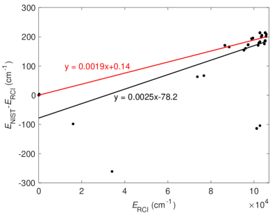
Figure 1: The energy differences along with present computed excitation energies. The black solid line is the linear fit to the scatter data shown in the figure. The red solid line is the linear fit by excluding the $2s^{2}2p^{4}\leavevmode\nobreak\ {}^{1}D_{2}$, ${}^{1}S_{0}$, $2s^{2}2p^{3}3s\leavevmode\nobreak\ ^{5}S_{2}$, ${}^{3}S_{1}$, ${}^{3}D_{1,2,3}$, and ${}^{1}D_{2}$ states.

The energies for the 81 lowest states of O i (45 even states and 36 odd states) are given in Table 7. In the calculations, the labelling of the eigenstates is determined by the CSF with the largest coefficient in the expansion of Eq. (1). For comparison, the observed energies from the NIST-ASD (Kramida et al., 2022), together with the differences $\Delta E$ = $E_{\rm{NIST}}$ - $E_{\rm{MCDHF}}$ are aslo displayed in the table. In most cases, the relative differences between theoretical and experimental results are less than 0.2%, with the exception of the levels belonging to the ground configuration ${2s^{2}2p^{4}}$, for which the average relative difference is about 1.16%. Fig. 1 shows the energy differences between NIST-ASD values and the present computed data, $\Delta E$, plotted against the excitation energies, $E\mathrm{{}_{RCI}}$. From the linear fitting we can see that the computational excitation energies have a systematic error of 0.25%. We observed that for most of the levels, the computed results are smaller than the NIST-ASD values by about 170-190 cm^-1 except for a few states belonging to $2s^{2}2p^{4}$ and $2s^{2}2p^{3}3s$. By excluding these levels, that is, $2s^{2}2p^{4}\leavevmode\nobreak\ {}^{1}D_{2}$, ${}^{1}S_{0}$, $2s^{2}2p^{3}3s\leavevmode\nobreak\ ^{5}S_{2}$, ${}^{3}S_{1}$, ${}^{3}D_{1,2,3}$, and ${}^{1}D_{2}$, the systematic error decreased to 0.19%. In the last two columns of Table 7, lifetimes obtained from the computed E1 transition rates in both Babushkin and Coulomb gauges are also presented. The relative differences between the Babushkin and Coulomb gauges are well below 5%, except for a few states for which decay to the lower states is dominated by intercombination transitions.

In Table 2, the lifetimes from the present MCDHF/RCI calculations are compared with available results from other theoretical calculations and experimental measurements. The calculated lifetimes in the Babuskin and Coulomb forms are consistent to 6.0% for all the selected transitions. Among others, atomic properties of the metastable state ${2p^{3}3s\leavevmode\nobreak\ ^{5}S^{o}_{2}}$ are interesting due to its potential in astrophysical diagnosis. The lifetime of the ${2p^{3}3s\leavevmode\nobreak\ ^{5}S^{o}_{2}}$ state has been studied systematically using the MCDHF method by Zhang et al. (2020) and the final values of 202$\pm$30 $\mu$s in the Babuskin gauge and 235$\pm$35 $\mu$s in the Coulomb gauge were recommended. Our calculated results of 209/213 $\mu$s (in B/C forms) are in good agreement with their values. The much larger lifetime from the MCHF calculation by Tachiev & Froese Fischer (2002) is likely caused by neglected electron correlation and relativistic effects. However, the theoretical lifetimes from the various calculations are still larger than the experimental values reported in Wells & Zipf (1974), Johnson (1972), Nowak et al. (1978), and Mason (1990), obtained using the time-of-flight technique. It is also interesting to note that the theoretical lifetimes from Tayal (2009), based on the B-spline box-based R-matrix method, for ${3s\leavevmode\nobreak\ ^{3}D^{o}}$, ${4s\leavevmode\nobreak\ ^{3}S^{o}}$, ${4d\leavevmode\nobreak\ ^{5}D^{o}}$, and ${4d\leavevmode\nobreak\ ^{3}D^{o}}$ states, differ significantly from those obtained with the other three theoretical approaches, which are Tachiev & Froese Fischer (2002) using the MCHF method implemented in the ATSP code (Froese Fischer, 2000; Froese Fischer et al., 2007), and the configuration interaction (CI) calculations of Hibbert et al. (1991) and Biemont & Zeippen (1992) that were made with the CIV3 (Hibbert, 1975) and SUPERSTRUCTURE codes (Eissner, W., 1991), respectively.

There are a number of measurements of lifetimes in O i presented in, for example, Brooks et al. (1977) using the electron-beam phase-shift method, Kröll et al. (1985) from the time-resolved laser spectroscopy, and Smith et al. (1971); Pinnington et al. (1974) using the beam foil technique. The measurements of Brooks et al. (1977) agree within the experimental errors with our calculated lifetimes for 3$s\leavevmode\nobreak\ {{}^{3}S^{o},^{3}D^{o}}$, and $5d\leavevmode\nobreak\ {{}^{3}D^{o}}$ states, while showing large discrepancies for $4s,5s\leavevmode\nobreak\ {{}^{3}S^{o}}$ and $4d\leavevmode\nobreak\ {{}^{3}D^{o}}$ states. Our lifetimes of $3s\leavevmode\nobreak\ ^{3}S^{o},^{3}D^{o}$, and ${}^{1}D^{o}$ states agree well with the experimental results published by Smith et al. (1971) using the beam-foil method; while Pinnington et al. (1974), which utilized the same experimental technique, measured somewhat larger values. Time-resolved spectroscopy and high frequency deflection technique were used, respectively, by Kröll et al. (1985) and Bromander et al. (1978) for measuring the lifetimes of ns, np and nd states in O i. The results from Kröll et al. (1985) are consistent with our theoretical lifetimes within the experimental errors; while the results from Bromander et al. (1978) are either too large or too small, when compared with the theoretical predicted values. For $3s\leavevmode\nobreak\ {{}^{3}S^{o}}$ state, our results agree well with all the experimental data if we exclude the lifetime from Savage & Lawrence (1966), which is evidently too large.

Table 2: Comparison of lifetimes in both Babushkin (B) and Coulomb (C) gauges, B/C, with other theoretical (Other Theo.) and experimental (Exp.) results.

		lifetime
State	Unit	Present		Other Theo.		Exp.
${2p^{3}3s\leavevmode\nobreak\ ^{5}S^{o}}$	$\mu$s	209/213		528a, 202/235d, 200e		170$\pm$25f, 185$\pm$10g,
						180$\pm$5h, 185$\pm$30i
${2p^{3}3s\leavevmode\nobreak\ ^{3}S^{o}}$	ns	1.70/1.69		1.76a,1.61b, 1.73c, 1.63e		2.4$\pm$0.3j, 1.7$\pm$0.3k, 1.7$\pm$0.2l, 1.82$\pm$0.05r,
						1.79$\pm$0.17p, 1.70$\pm$0.15m, 1.70$\pm$0.14n, 1.8$\pm$0.27o
${2p^{3}3s\leavevmode\nobreak\ ^{3}D^{o}}$	ns	4.21/4.15		4.19b, 4.46c		3.94$\pm$0.22p, 5.0$\pm$0.4q, 4.5$\pm$0.675o
${2p^{3}3s\leavevmode\nobreak\ ^{1}D^{o}}$	ns	1.86/1.85				1.77$\pm$0.14p, 2.01$\pm$0.12q
${2p^{3}4s\leavevmode\nobreak\ ^{3}S^{o}}$	ns	5.74/5.67		5.33a, 5.24b, 5.04c		4.0$\pm$0.6o
${2p^{3}5s\leavevmode\nobreak\ ^{3}S^{o}}$	ns	13.55/13.35				17$\pm$3s, 6.0$\pm$0.9o
${2p^{3}6s\leavevmode\nobreak\ ^{3}S^{o}}$	ns	26.82/25.22				24$\pm$3s
${2p^{3}3p\leavevmode\nobreak\ ^{3}P}$	ns	32.12/32.73		32.70a, 29.68b		36$\pm$4s, 39.1$\pm$1.4t, 40$\pm$3u
${2p^{3}4p\leavevmode\nobreak\ ^{3}P}$	ns	182.3/181.8		175.4b		153$\pm$10u, 161$\pm$19v
${2p^{3}4p\leavevmode\nobreak\ ^{5}P}$	ns	200.2/212.0		189.7b		193$\pm$10u, 194$\pm$19v
${2p^{3}4d\leavevmode\nobreak\ ^{5}D^{o}}$	ns	72.15/73.21		72.20b, 96.64c		96$\pm$4u, 95$\pm$9v
${2p^{3}4d\leavevmode\nobreak\ ^{3}D^{o}}$	ns	15.31/15.41		16.85b, 12.91c		23$\pm$3s, 20$\pm$3o, 80$\pm$10u
${2p^{3}5d\leavevmode\nobreak\ ^{3}D^{o}}$	ns	31.13/32.12				36$\pm$4s, 30$\pm$4.5o

3.2 Transition rates and oscillator strengths

Transition data in the form of wavelengths, line strengths (S), weighted oscillator strengths (log($gf$)), transition probabilities ($A$), gauge agreements, d$T$, cancellation factors, CF, as well as the estimated accuracy classes of all computed E1 transitions are given in Table 8. It is important to note that the reported wavelengths have been adjusted to match the level energy values in the NIST-ASD. The data for log($gf$) and A are reported in both Babuskin and Coulomb gauge and are adjusted using experimental wavelengths.

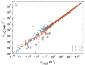
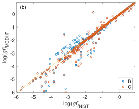
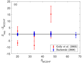
Figure 2: Comparison of transition data of the current study with the values from other work. Panel (a): Comparison of theoretical transition probabilities, $A$, in both Babushkin (B) and Coulomb (C) gauge with the results available in the NIST-ASD (Kramida et al., 2022). Panel (b): Comparison of the log($gf$) values in Babushkin form with the results from CIV3 (Hibbert et al., 1991), MCHF (Tachiev & Froese Fischer, 2002) and B-spline R-matrix (Tayal, 2009) calculations. Panel (c): Comparison of the theoretical line strengths, $S\mathrm{{}_{MCDHF}}$, with the corresponding experimental results published by Golly et al. (2003) (in red square) and Bacławski (2008) (in blue circle). Note that relative line strengths were provided by Bacławski (2008), which means that the line strengths are normalised within each multiplet to the sum of 100; the corresponding results from present calculations and Golly et al. (2003) are done with the same procedure. The line strengths in Babushkin gauge are used for the comparison.

3.2.1 Comparisons with previous theoretical results

The calculated transition results are compared with other theoretical works. In the left panel of Fig. 2, $A$ values in both Babushkin and Coulomb gauges from the present work are compared with available data from the NIST-ASD (Kramida et al., 2022), which are compiled based on the results from Hibbert et al. (1991), Biemont & Zeippen (1992), and Butler & Zeippen (1991). The first two calculations were carried out using the CIV3 and SUPERSTRUCTURE code, respectively. The latter work was done within the framework of the international Opacity Project.

As shown in the figure, the agreement between the $A$ values computed in the present work and the respective results from the NIST-ASD is rather good for most transitions, especially for transitions with $A_{\mathrm{B}}$ $\geq$ 10⁵ s^-1; taking results in Babuskin gauge as example, 70% of the 380 selected transitions are in agreement with the NIST-ASD data with the differences less than 20%. 204 out of the 236 transitions having $A_{\mathrm{B}}$ $\geq$ 10⁵ are in agreement with the NIST-ASD data with the relative differences less than 10%. It is interesting to note that, for transitions with 10³ $\leq A\leq$ 10⁵ s^-1, the transition data in the Coulomb gauge are more consistent with the results in the NIST-ASD than those in the Babushkin gauge. On closer inspection of these transitions we found that most of them are transitions involving high Rydberg states. For example, 74% of them are those from $n$ = 5, 6 states to lower levels. For this class of transitions we recommend the radiative data calculated in the Coulomb gauge, and not the more conventional Babuskin gauge. Following Papoulia et al. (2019), the reason for this is that correlation orbitals resulting from MCDHF calculations based on CSF expansions obtained by including substitutions from deeper subshells are contracted in comparison with the outer Rydberg orbitals. As a consequence, the outer parts of the wavefunctions for the relatively extended Rydberg states are not accurately described. Thus, it can be argued that the Coulomb gauge, which is weighted on the inner parts of the wavefunction, should yield more reliable transition data than the Babushkin gauge for transitions involving high-lying Rydberg states. However, for transitions involving low-lying states, our calculated transition rates in two gauges are very consistent with each other, except for some weak transitions with $A$ ¡ 10² s^-1; for these transitions with large differences between two gauges, the Babushkin form is generally preferred, since it is more sensitive to the outer part of the wave functions that governs the atomic transitions (Grant, 1974; Hibbert, 1974).

Furthermore, in the middle panel of Fig. 2, the computed log($gf$) values in the Babushkin gauge are compared with the results from various calculations of Tayal (2009), Tachiev & Froese Fischer (2002), and Hibbert et al. (1991), which were carried out by B-spline R-matrix, CI and MCHF methods, respectively. From the figure, we note an excellent agreement between the present results and the other three theoretical values for transitions with log($gf$) ¿ $-$1.5. However, for weaker transitions with log($gf$) ¡ $-$1.5, agreement between different methods is worse with a much wider scatter. Overall, the log($gf$) values from the present work are in better agreement with those from Tachiev & Froese Fischer (2002) and Hibbert et al. (1991) than those from Tayal (2009).

Table 3: Comparison of $gf$ values in both Babushkin (B) and Coulomb (C) gauges, B/C, with available experimental (Exp.) results.

							$gf$
Upper	Lower	$\lambda_{\text{vac.}}$(nm)	Present		Exp.a		Other Exp.
${2p^{3}3s\leavevmode\nobreak\ ^{3}S^{o}_{1}}$	${2p^{4}\leavevmode\nobreak\ {}^{3}P_{0}}$	130.603	0.0499/0.0501				0.05$\pm$0.01b, 0.05$\pm$0.005c, 0.047$\pm$0.0014d,
							0.047$\pm$0.0047e, 0.048$\pm$0.0048f, 0.050$\pm$0.0050g,
							0.05$\pm$0.0115h, 0.052$\pm$0.0052i,
							0.045$\pm$0.009j, 0.053$\pm$0.00318k
${2p^{3}3s\leavevmode\nobreak\ ^{1}D^{o}_{2}}$	${2p^{4}\leavevmode\nobreak\ {}^{1}D_{2}}$	115.215	0.535/0.538		0.49$\pm$0.039		0.526$\pm$0.083b, 0.526$\pm$0.055d, 0.56$\pm$0.04e,
							0.50$\pm$0.05f, 0.51$\pm$0.026g, 0.50$\pm$0.03l
${2p^{3}4s\leavevmode\nobreak\ ^{3}S^{o}_{1}}$	${2p^{4}\leavevmode\nobreak\ {}^{3}P_{0}}$	104.169	0.00827/0.00841		0.0089$\pm$0.0015
${2p^{3}4s\leavevmode\nobreak\ ^{3}S^{o}_{1}}$	${2p^{4}\leavevmode\nobreak\ {}^{3}P_{1}}$	104.094	0.0249/0.0252		0.029$\pm$0.0049
${2p^{3}4s\leavevmode\nobreak\ ^{3}S^{o}_{1}}$	${2p^{4}\leavevmode\nobreak\ {}^{3}P_{2}}$	103.923	0.0417/0.0423		0.048$\pm$0.0072
${2p^{3}3d\leavevmode\nobreak\ ^{3}D^{o}_{1,2}}$	${2p^{4}\leavevmode\nobreak\ {}^{3}P_{1}}$	102.743	0.0627/0.0624		0.069$\pm$0.010
${2p^{3}3d\leavevmode\nobreak\ ^{3}D^{o}_{1}}$	${2p^{4}\leavevmode\nobreak\ {}^{3}P_{0}}$	102.816	0.0209/0.0208		0.024$\pm$0.0031
${2p^{3}3s\leavevmode\nobreak\ ^{3}D^{o}_{1}}$	${2p^{4}\leavevmode\nobreak\ {}^{3}P_{0}}$	99.080	0.0570/0.0577		0.052$\pm$0.0047
${2p^{3}3s\leavevmode\nobreak\ ^{3}D^{o}_{1}}$	${2p^{4}\leavevmode\nobreak\ {}^{3}P_{1}}$	99.013	0.0442/0.0448		0.042$\pm$0.0042
${2p^{3}3s\leavevmode\nobreak\ ^{3}D^{o}_{2}}$	${2p^{4}\leavevmode\nobreak\ {}^{3}P_{1}}$	99.020	0.128/0.130		0.11$\pm$0.0121
${2p^{3}3s\leavevmode\nobreak\ ^{3}D^{o}_{2}}$	${2p^{4}\leavevmode\nobreak\ {}^{3}P_{2}}$	98.865	0.0457/0.0463		0.051$\pm$0.0071
${2p^{3}3s\leavevmode\nobreak\ ^{3}D^{o}_{3}}$	${2p^{4}\leavevmode\nobreak\ {}^{3}P_{2}}$	98.877	0.243/0.246		0.22$\pm$0.044

3.2.2 Comparisons with available experimental results

In Table 3, the computed $gf$ values are compared with some available results from experimental measurements. Goldbach & Nollez (1994) measured the log($gf$) values of 12 lines of O i belonging to 5 multiplets in the 95-120 nm spectral range with a wall-stabilized arc. The uncertainty achieved in the measured absolute $gf$-values is between $\pm$10 and $\pm$20%. Our computed $gf$ results in both gauges are in excellent agreement with the measured values by Goldbach & Nollez (1994), except for the 115.215 nm and 99.080 nm lines, for which we predict slightly larger values (by 2%). For the 115.215 nm line, other determinations of $gf$ value have also been achieved by utilizing various techniques, for instance, beam-foil technique (Smith et al., 1971; Martinson et al., 1971; Lin et al., 1972; Pinnington et al., 1974), phase-shift technique (Gaillard & Hesser, 1968), or pulsed electron beam (Lawrence, 1970). From Table 3 we notice that different methods obtained very consistent results, and our computed values are in nice agreement with them. A number of measurements of $gf$ values have also been done for the 130.6 nm line. Again, the results from different measurements agree perfectly with each other, as well as with our computed results in both Babushkin and Coulomb gauges. In addition, Bridges & Wiese (1998) measured the transition probabilities of the $2p^{3}3s\leavevmode\nobreak\ ^{3}S^{o}-4p\leavevmode\nobreak\ ^{3}P$ and $3s\leavevmode\nobreak\ ^{5}S^{o}-2p^{3}4p\leavevmode\nobreak\ ^{5}P$ arrays and obtained the values of 7.62 $\times 10^{5}$ s^-1 and 3.64 $\times 10^{5}$ s^-1, respectively. Our computed results are in agreement with the experimental value for the $2p^{3}3s\leavevmode\nobreak\ ^{3}S^{o}-2p^{3}4p\leavevmode\nobreak\ ^{3}P$ array within the experimental error, while predict slightly larger transition probability for the $2p^{3}3s\leavevmode\nobreak\ ^{5}S^{o}-2p^{3}4p\leavevmode\nobreak\ ^{5}P$ array, that is, by about 5% after considering the experimental uncertainty.

There are also measurements of line strengths for spectral lines in visible and infrared (Golly et al., 2003; Bacławski, 2008). In Fig. 2 (c), the computed $S$ values in Babushkin gauge are compared with experimental results from Golly et al. (2003) and Bacławski (2008), by plotting line strength differences versus the computed line strengths. Note that Bacławski (2008) provided the relative line strengths within multiplets (normalised to 100); therefore all the values used for comparison in Fig. 2 (c) are converted to the relative values. We can see that all of our computed lines strengths are in agreement with the results from Bacławski (2008) within the reported experimental uncertainties. However, in comparison with the results by Golly et al. (2003), large discrepancies are observed for the $2p^{3}3p\leavevmode\nobreak\ ^{5}P-2p^{3}3d\leavevmode\nobreak\ ^{5}D^{o}$ transition array, for which our computed results are in perfect agreement with those from Bacławski (2008).

3.2.3 Uncertainty estimation using d$T$ and CF

Table 4: Distribution of d$T$ (in %) and CF of the computed transition rates in O i depending on the magnitude of the transition rates. The analysis is done based on the data adjusted to experimental wavelengths.

Group	$A$	No.	$\langle\rm{d}\it{T}\rangle$	$\rm{d}\it{T}$ ¡ 20% (& CF ¿ 0.05)	$\rm{d}\it{T}$ ¡ 10% (& CF ¿ 0.05)	$\rm{d}\it{T}$ ¡ 5% (& CF ¿ 0.05)
	(s-1)		(%)	(%)	(%)	(%)
g1	100–102	226	28.32	58.8 (0.4)	38.1 (0.4)	23.5 (0.0)
g2	102–104	147	17.03	74.8 (24.5)	72.1 (23.1)	57.1 (12.2)
g3	104–106	221	17.99	75.6 (65.2)	63.3 (54.3)	52.5 (45.7)
g4	106–	166	2.29	100.0 (95.8)	98.8 (94.6)	86.7 (82.5)

Table 5: The connection of the limits of d$T$ or d$\tilde{T}$ and CF for the accuracy classes (Acc.).

Acc.	Unc.	d$T$ or d$\tilde{T}$	CF	$N$	$N_{\mathrm{acc.}}$
	(%)	(%)			g1	g2	g3	g4
A	$\leq$ 3	$\leq$ 3	$\geq$ 0.1	80	0	0	0	80
B	$\leq$ 10	¿ 3 & $\leq$ 10	$\geq$ 0.1	125	0	0	41	84
		$\leq$ 3	¡ 0.1
C	$\leq$ 25	¿ 10 & $\leq$ 25	$\geq$ 0.1	317	70	111	134	2
		¿3 & $\leq$ 10	¡ 0.1
D	$\leq$ 50	¿ 25 & $\leq$ 50	$\geq$ 0.1	269	110	20	19	0
		or ¿10 & $\leq$ 25	¡ 0.1
E	$>$ 50	¿ 50		198	46	16	27	0
		¿ 25 & $\leq$ 50	¡ 0.1

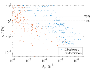
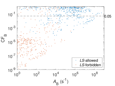
Figure 3: Scatterplot of d$T$ and CF values versus transition rates $A$ of E1 transitions, for O i. Left panel: Scatterplot of d$T$ values versus transition rates in Babushkin form, $A_{\rm{B}}$, of E1 transitions with $A_{\rm{B}}$ ¿ 10⁰ s^-1. Right panel: Same as the left panel but for cancellation factor, CF. $LS$-allowed and $LS$-forbidden transitions are marked in blue and red, respectively.

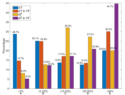
Figure 4: Percentage fractions of all transitions in O i in different uncertainty categories: A (Uncertainty $\leq$ 3%), B (3% $<$ Uncertainty $\leq$ 10%), C (10% $<$ Uncertainty $\leq$ 25%), D (25% $<$ Uncertainty $\leq$ 50%), and E (Uncertainty $>$ 50%), for the uncertainty estimate based on d$T$ values only (blue), d$T$&CF values (red), d$\tilde{T}$ (orange), and d$\tilde{T}$&CF values (purple).

There are a number of methods being used for estimation of uncertainties of calculated transition rates (Kramida, 2014; Froese Fischer, 2009; Ekman et al., 2014; El-Sayed, 2021; Gaigalas et al., 2020). However, the estimation of uncertainties of calculated transition rates is not trivial and different methods may only applicable to specific systems and ionisation stages. In this work, as discussed in Sec. 2.2 (see Eqs. (3) and (4)), we attempted to evaluate the uncertainties using the d$T$ and CF values.

Fig. 3 shows the scatterplots of d$T$ (left panel) and CF (right panel, in Babushkin gauge) versus $A$ (in Babushkin gauge). Note that the weak transitions with transition rates $A$ ¡ 10⁰ s^-1 are neglected in the figure due to the fact that these weak transitions tend to be of lesser astrophysical importance, either for opacity calculations, or for spectroscopic abundance analyses. In the figure, we depict the $LS$-allowed and $LS$-forbidden transitions in different colours. Overall, as can be seen from Fig. 3, stronger transitions with larger $A$ rates or $LS$-allowed transitions are always associated with smaller d$T$ and larger CF values, which indicate that these transitions have small uncertainties. However, the weak transitions, which are mostly the $LS$-forbidden intercombination transitions, are associated with smaller CFs and are strongly affected by cancellations. The mean d$T$ (CF) for all E1 transitions shown in Fig. 3 is 17.4% (0.27).

To better display the d$T$ and CF parameters of the computed transitions rates and their distribution in relation to the magnitude of the transition rates $A$, we organised the transitions into four groups (g1 - g4) based on the magnitude of $A$ values, as shown in Table 4. The first three groups contain the weak transitions with $A$ up to 10⁶ s^-1, while the last group contains the strong transitions with $A\geq$ 10⁶ s^-1. The average value of the $\langle\rm{d}\it{T}\rangle$ is given for each group. The $\langle\rm{d}\it{T}\rangle$ is only 2.29% for the fourth group transition, which indicates a very high accuracy achieved for the strong transitions with $A\geq$ 10⁶ s^-1. In addition, the statistical analysis of the proportions of transitions with CF ¿ 0.05 and/or different d$T$ values, that is, d$T$ ¡ 20%, d$T$ ¡ 10%, and d$T$ ¡ 5%, for each group of transitions is also performed and shown in the last three columns of Table 4.

Based on the d$T$ and CF values, we estimated the accuracy class for each transition using four procedures. The first one adopts the d$T$ value defined in Eq. (3) as the uncertainty for each transition rate. For the second procedure, the definition of d$T$ and CF for each of the accuracy classes are presented in Table 5. Furthermore, in the third approach, we organised the transitions into six groups based on the magnitude of $A$ values, that is, $A$ ¡ 10^-2 s^-1, 10^-2 $\leq A$ ¡ 10¹ s^-1, 10¹ $\leq A$ ¡ 10³ s^-1, 10³ $\leq A$ ¡ 5$\times$10⁵ s^-1, 5$\times$10⁵ $\leq A$ ¡ 3.5$\times$10⁶ s^-1, and $A\geq$ 3.5$\times$10⁶, and calculated the averaged d$T_{\mathrm{av}}$ for each group. Then we defined d$\tilde{T}$ = max(d$T$, d$T_{\mathrm{av}}$) to replace the d$T$ as the uncertainty of each particular transition rate. Finally, the fourth procedure employs the definition of d$\tilde{T}$ and CF given in Table 5 as the uncertainty indicator. The statistical analysis of the number of transitions belonging to a specific accuracy class is performed. The percentage fractions obtained from the four methods are shown in Fig. 4.

From the comparison between the d$T$ and d$T\&$CF methods, we can see that the accuracy of some of the A class transitions is degraded according to the value of CF, for example, the percentage fraction is decreased from 28.7% to 14.7% for the A class transitions. Compared to the other two indicators, d$\tilde{T}$ and d$\tilde{T}\&$CF predicted rather low percentage fractions of transitions in high-accuracy category having uncertainties less than 10%, which are 8.0% and 5.2%, respectively. From Fig. 4, using the d$T$ values only for accuracy estimations might underestimate the uncertainties. As concluded in Ekman et al. (2014), d$T$ is a reliable indicator of uncertainties of transition rates, especially for $LS$-allowed transitions; while for $LS$-forbidden transitions, d$T$ can be used as uncertainties indicators if averaging over a large sample. Therefore, the d$\tilde{T}$ and d$\tilde{T}\&$CF indicators may yield a ”safer” uncertainty estimation of the calculated transition rates, although they may overestimate the uncertainties, especially for the strong $LS$-allowed transitions.

The accuracy classes predicted from the d$\tilde{T}$ procedure are given in Table 8. A statistical analysis is performed on the distributions of accuracy classes, and the results are shown in Table 5. Overall, 80 (205) out of 989 computed transitions in this work have a uncertainty of ¡ 3% (¡ 10%) and assigned to accuracy class A (B). Among the 80 transitions belonging to the A accuracy class, all are rather strong, with $A\geq$ 10⁶ s^-1 (g4). All the transitions in g4 are associated with uncertainties less than 25%; while for group g1, most transitions are assigned to accuracy classes C, D or E.

4 The solar oxygen abundance

The solar oxygen abundance is still under heated debate. It has undergone a major downward revision in the past decades, from $\log{\epsilon_{\mathrm{O}}}\equiv\log{N_{\mathrm{O}}/N_{\mathrm{H}}}+12$ = 8.93 in Anders & Grevesse (1989) to 8.66 in Asplund et al. (2005). Recent estimates can be separated into “low” values of $\log{\epsilon_{\mathrm{O}}}$ = 8.67-8.71 (Amarsi et al., 2018, 2021; Asplund et al., 2021), and “intermediate” values of 8.73-8.77 (Caffau et al., 2015; Steffen et al., 2015; Bergemann et al., 2021; Magg et al., 2022), with “high” values in the range 8.80-8.90 sometimes also suggested (Socas-Navarro, 2015; Cubas Armas et al., 2020).

Table 6: Allowed O i lines used as oxygen abundance diagnostics.

			$\log gf$
Upper	Lower	$\lambda_{\text{air}}$(nm)	Present		NIST(a)	QDT(b)	Multi-method(c)	Multi-method(d)
			B	C
${2p^{3}4d\leavevmode\nobreak\ ^{5}D_{2}^{o}}$	${2p^{3}3p\leavevmode\nobreak\ ^{5}P_{3}}$	615.815	-1.849	-1.851	-1.841
${2p^{3}4d\leavevmode\nobreak\ ^{5}D_{3}^{o}}$	${2p^{3}3p\leavevmode\nobreak\ ^{5}P_{3}}$	615.817	-1.004	-1.006	-0.995
${2p^{3}4d\leavevmode\nobreak\ ^{5}D_{4}^{o}}$	${2p^{3}3p\leavevmode\nobreak\ ^{5}P_{3}}$	615.819	-0.418	-0.420	-0.409
${2p^{3}3p\leavevmode\nobreak\ ^{5}P_{3}}$	${2p^{3}3s\leavevmode\nobreak\ ^{5}S_{2}^{o}}$	777.194	0.350	0.335	0.369	0.317	0.350	0.350$\pm$0.021
${2p^{3}3p\leavevmode\nobreak\ ^{5}P_{2}}$	${2p^{3}3s\leavevmode\nobreak\ ^{5}S_{2}^{o}}$	777.417	0.204	0.189	0.223	0.170	0.204	0.196$\pm$0.022
${2p^{3}3p\leavevmode\nobreak\ ^{5}P_{1}}$	${2p^{3}3s\leavevmode\nobreak\ ^{5}S_{2}^{o}}$	777.539	-0.018	-0.033	0.002	-0.051	-0.019	-0.0296$\pm$0.021
${2p^{3}3p\leavevmode\nobreak\ ^{3}P_{0}}$	${2p^{3}3s\leavevmode\nobreak\ ^{3}S_{1}^{o}}$	844.625	-0.466	-0.474	-0.463	-0.493
${2p^{3}3p\leavevmode\nobreak\ ^{3}P_{2}}$	${2p^{3}3s\leavevmode\nobreak\ ^{3}S_{1}^{o}}$	844.636	0.233	0.225	0.236	0.206
${2p^{3}3p\leavevmode\nobreak\ ^{3}P_{1}}$	${2p^{3}3s\leavevmode\nobreak\ ^{3}S_{1}^{o}}$	844.676	0.011	0.003	0.014	-0.015
${2p^{3}3d\leavevmode\nobreak\ ^{5}D_{2}^{o}}$	${2p^{3}3p\leavevmode\nobreak\ ^{5}P_{3}}$	926.583	-0.739	-0.737	-0.718	-0.750
${2p^{3}3d\leavevmode\nobreak\ ^{5}D_{3}^{o}}$	${2p^{3}3p\leavevmode\nobreak\ ^{5}P_{3}}$	926.594	0.106	0.108	0.125	0.096
${2p^{3}3d\leavevmode\nobreak\ ^{5}D_{4}^{o}}$	${2p^{3}3p\leavevmode\nobreak\ ^{5}P_{3}}$	926.601	0.693	0.694	0.712	0.681
${2p^{3}4s\leavevmode\nobreak\ ^{5}S_{2}^{o}}$	${2p^{3}3p\leavevmode\nobreak\ ^{5}P_{3}}$	1130.238	0.056	0.040	0.078	0.033
${2p^{3}4s\leavevmode\nobreak\ ^{3}S_{1}^{o}}$	${2p^{3}3p\leavevmode\nobreak\ ^{3}P_{1}}$	1316.389	-0.258	-0.263	-0.254	-0.280
${2p^{3}4s\leavevmode\nobreak\ ^{3}S_{1}^{o}}$	${2p^{3}3p\leavevmode\nobreak\ ^{3}P_{2}}$	1316.485	-0.036	-0.041	-0.032	-0.058
${2p^{3}4s\leavevmode\nobreak\ ^{3}S_{1}^{o}}$	${2p^{3}3p\leavevmode\nobreak\ ^{3}P_{0}}$	1316.511	-0.735	-0.740	-0.731	-0.757

One of the differences between the recent studies of Amarsi et al. (2018) and Asplund et al. (2021) (low oxygen abundances) and Bergemann et al. (2021) and Magg et al. (2022) (intermediate oxygen abundances) are the transition probabilities for their O i lines. In the former case, the transition probabilities for the O i 615.8 nm, 777 nm, 844.7 nm and 926.9 nm features were taken from the NIST-ASD and are based on the atomic data of Hibbert et al. (1991). On the other hand, the latter two studies, based solely on the O i 777 nm triplet, draw on calculations from Civiš et al. (2018) computed using the quantum defect theory (QDT), as well as from Bautista et al. (2022) based on an average over results from multiple methods.

Table 6 presents the the permitted lines that have been adopted by different solar oxygen abundance analyses (Asplund et al., 2004; Caffau et al., 2008; Asplund et al., 2021) . The log($gf$) values for these lines from various calculations are given in the table. It is interesting to note that, in all cases, the log($gf$) values from the NIST-ASD (based on Hibbert et al. 1991) are systematically larger than the other theoretical results. Compared to our results in the Babushkin gauge, they are between $0.01$ to $0.02\,\mathrm{dex}$ too small. Also, the QDT values of Civiš et al. (2018) are systematically smaller than the values from the other calculations; the differences with our results are between $0.01$ to $0.03\,\mathrm{dex}$. In both cases, the differences are the largest for the O i 777 nm triplet.

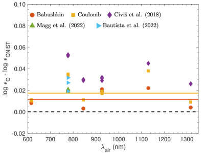
Figure 5: Solar oxygen abundance differences inferred using different theoretical transition data given in Table 6, relative to the NIST-ASD values. Red circle: Babushkin gauge from present work. Orange square: Coulomb gauge from present work. Purple diamond: Civiš et al. (2018). Green up triangle: Magg et al. (2022). Blue right triangle: Bautista et al. (2022). Red and blue solid horizontal lines illustrate the mean result for the Babushkin gauge and Coulomb gauge, respectively. Note we give equal weights to all $LS$ features.

Fig. 5 illustrates the results in Table 6 in terms of differences to the solar oxygen abundance via

$$\rm\Delta log\leavevmode\nobreak\ \epsilon=-\Delta\leavevmode\nobreak\ log\leavevmode\nobreak\ (\it gf)=-\left(\rm log\leavevmode\nobreak\ (\it gf)_{\rm new}-\rm log\leavevmode\nobreak\ (\it gf)_{\rm orig}\right),$$ (5)

where in this case $\rm log\leavevmode\nobreak\ (\it gf)_{\rm orig}$ corresponds to the log($gf$) values from Hibbert et al. (1991) via the NIST-ASD. One sees a systematic shift upwards, by $0.01{{\color[rgb]{0,0,0}1}}\,\mathrm{dex}$ on average in the Babushkin gauge, and $0.01{{\color[rgb]{0,0,0}7}}\,\mathrm{dex}$ on average in the Coulomb gauge. In particular, for the O i 777 nm triplet, to which Asplund et al. (2021) gave the largest weight among their selected atomic lines and for which they adopt $\log{\epsilon_{\mathrm{O}}}$= 8.69 via the analysis of Amarsi et al. (2018), the inferred abundance increases to $\log{\epsilon_{\mathrm{O}}}$ = 8.71. This value remains in good agreement with the one those authors obtained from forbidden lines (8.70) and from molecular lines (8.70; see also Amarsi et al. 2021), and within the quoted uncertainty of $0.04$.

The result of Amarsi et al. (2018) for the O i 777 nm triplet is $0.06-0.08\,\mathrm{dex}$ lower than that found by Bergemann et al. (2021) (8.75$\pm$0.03) and Magg et al. (2022) (8.77$\pm$0.04) from the same spectral feature. As illustrated in Fig. 5, the difference in $\rm log\leavevmode\nobreak\ (\it gf)$ from the multi-method results of Magg et al. (2022) and Bautista et al. (2022), compared to that adopted in Amarsi et al. (2018), amounts to around $0.02-0.03\,\mathrm{dex}$. These differences are significant, but they are not the dominant reason for the $0.06-0.08\,\mathrm{dex}$ discrepancies. Further discussion of the origins of these discrepancies may be found in Sec. 4.4 of Amarsi et al. (2021).

Our overall advocated solar oxygen abundance is $8.70\pm 0.04$, after taking into account permitted O i, forbidden [O i], and molecular OH lines, and adopting the same (systematic) uncertainty as given in Asplund et al. (2021). This falls in the “low” range of values as defined above, and does little to alleviate the solar modelling problem. Rather, the solution to this long-standing problem may in part derive from improvements to the theoretical modelling (Bailey et al., 2015; Buldgen et al., 2017, 2019; Zhang et al., 2019; Yang, 2019, 2022).

5 Conclusions

Extended atomic data including energy levels, lifetimes, and transition data of E1 transitions, are computed and provided for O i using MCDHF and RCI methods. These data are indispensable for reliable solar and stellar spectroscopic analyses.

We have performed extensive comparisons of the computed transition data with other theoretical and experimental results. The agreement between the computed transition data and the respective results from the NIST-ASD is rather good for most of the transitions, especially for transitions with $A$ $\geq$ 10⁵ s^-1 or log($gf$) ¿ -1.5. 266 out of the 380 selected transitions available in the NIST-ASD are in agreement with the latter within 20%. At the same time, for weaker transitions with $A$ ¡ 10⁵ or log($gf$) ¡ -1.5, the discrepencies between different theoretical methods display a much wider scatter. In particular, for transitions with 10³ $\leq A\leq$ 10⁵ s^-1 or -3.5 $\leq$ log($gf$) $\leq$ -2, the transition data in the Coulomb gauge are in better agreement with the other theoretical values than those in the Babushkin gauge; most of them are transitions involving high Rydberg states, for which we recommend the radiative data in the Coulomb gauge from this work. The computed lifetimes and oscillator strengths, log($gf$), have also been compared with available results from experimental measurements. Our computed values (in either gauge) are in overall good agreement with the measured values.

In addition, we used four methods to estimate the uncertainties of the computed transition probabilities, based on the relative differences of the computed transition rates in the Babushkin and Coulomb gauges, which is given by the quantity d$T$, and CF. Based on the accuracy classes predicted from max(d$T$, d$T_{\mathrm{av}}$), 205 out of 989 computed transitions are with uncertainty less than 10% and assigned to the accuracy classes A or B. All of the computed transitions belonging to the AA accuracy class are rather strong with $A\geq$ 10⁶ s^-1. All the transitions with $A\geq$ 10⁶ s^-1 are associated with uncertainties less than 25%; while for weak transitions with $A$ ¡ 10² s^-1 , most are assigned to accuracy classes D or E.

Finally, the impact of the new atomic data on oxygen abundance analyses was analysed by applying corrections $\rm\Delta log\leavevmode\nobreak\ \epsilon=-\Delta\leavevmode\nobreak\ log\leavevmode\nobreak\ (\it gf)$ to literature abundances.. In general, the transition probabilities for typical O i lines are underestimated by Civiš et al. (2018), and overestimated by Hibbert et al. (1991). For the O i 777 nm triplet the differences with respect to our results in the Babushkin gauge are $-0.03\,\mathrm{dex}$ and $+0.02\,\mathrm{dex}$, respectively. Our transition probabilities combined with the analysis of the O i 777 nm triplet presented by Amarsi et al. (2018) suggests $\log{\epsilon_{\mathrm{o}}}=8.71$ for the Sun. This is in excellent agreement with low-excitation forbidden lines as well as molecular lines, and, overall, we advocate $\log{\epsilon_{\mathrm{o}}}=8.70\pm 0.04$.

6 Acknowledgements

AMA gratefully acknowledges support from the Swedish Research Council (VR 2020-03940). MCL would like to acknowledge the support from the Guangdong Basic and Applied Basic Research Foundation (2022A1515110043). We would like to thank the anonymous referee for his/her useful comments that helped improve the original manuscript.

Appendix A Energy levels and transition data for O i.

Table 7: Energy levels (in cm^-1) and lifetimes (in s; given in Babushkin ($\tau_{B}$) and Coulomb ($\tau_{C}$) gauges) for O i.

No.	State		$E_{\mathrm{MCDHF}}$		$E_{\mathrm{NIST}}$		${\Delta E}$		$\tau_{B}$		$\tau_{C}$
1	${2s^{2}2p^{4}\leavevmode\nobreak\ {}^{3}P_{2}}$		0.00		0.000		0
2	${2s^{2}2p^{4}\leavevmode\nobreak\ {}^{3}P_{1}}$		155.73		158.265		2.54
3	${2s^{2}2p^{4}\leavevmode\nobreak\ {}^{3}P_{0}}$		223.26		226.977		3.72
4	${2s^{2}2p^{4}\leavevmode\nobreak\ {}^{1}D_{2}}$		15966.11		15867.862		-98.25
5	${2s^{2}2p^{4}\leavevmode\nobreak\ {}^{1}S_{0}}$		34053.62		33792.583		-261.04
6	${2s^{2}2p^{3}3s\leavevmode\nobreak\ ^{5}S_{2}^{o}}$		73705.01		73768.200		63.19		2.0918E-04		2.1296E-04
7	${2s^{2}2p^{3}3s\leavevmode\nobreak\ ^{3}S_{1}^{o}}$		76728.03		76794.978		66.95		1.7020E-09		1.6911E-09
8	${2s^{2}2p^{3}3p\leavevmode\nobreak\ ^{5}P_{1}}$		86455.25		86625.757		170.51		2.9107E-08		3.0123E-08
9	${2s^{2}2p^{3}3p\leavevmode\nobreak\ ^{5}P_{2}}$		86457.22		86627.778		170.56		2.9094E-08		3.0109E-08
10	${2s^{2}2p^{3}3p\leavevmode\nobreak\ ^{5}P_{3}}$		86460.80		86631.454		170.65		2.9070E-08		3.0085E-08
–	–		–		–		–		–		–

Table 8: Electric dipole transition data for O i.

Upper	Lower	$\lambda$ (nm)	$S$ (a.u. of a${}_{0}^{2}$e2)		$\mathrm{log}\leavevmode\nobreak\ gf$		$A\leavevmode\nobreak\ (\mathrm{s}^{-1})$		d$T$	CF
			B	C	B	C	B	C		B	C	Acc.
${2s^{2}2p^{3}5d\leavevmode\nobreak\ ^{3}D_{1}^{o}}$	${2s^{2}2p^{4}\leavevmode\nobreak\ {}^{3}P_{2}}$	94.8686	1.01E-03	9.82E-04	-3.489	-3.502	8.01E+05	7.77E+05	0.030	1.90E-03	3.71E-02	B
${2s^{2}2p^{3}5d\leavevmode\nobreak\ ^{3}D_{2}^{o}}$	${2s^{2}2p^{4}\leavevmode\nobreak\ {}^{3}P_{2}}$	94.8686	1.52E-02	1.47E-02	-2.313	-2.327	7.20E+06	6.98E+06	0.030	3.84E-03	1.40E-01	B
${2s^{2}2p^{3}5d\leavevmode\nobreak\ ^{3}D_{3}^{o}}$	${2s^{2}2p^{4}\leavevmode\nobreak\ {}^{3}P_{2}}$	94.8686	8.48E-02	8.23E-02	-1.566	-1.579	2.87E+07	2.79E+07	0.030	8.04E-03	3.74E-01	A
${2s^{2}2p^{3}5d\leavevmode\nobreak\ ^{5}D_{3}^{o}}$	${2s^{2}2p^{4}\leavevmode\nobreak\ {}^{3}P_{2}}$	94.8898	1.37E-06	1.38E-06	-6.356	-6.354	4.66E+02	4.68E+02	0.006	1.32E-07	6.21E-06	C
${2s^{2}2p^{3}5d\leavevmode\nobreak\ ^{5}D_{2}^{o}}$	${2s^{2}2p^{4}\leavevmode\nobreak\ {}^{3}P_{2}}$	94.8898	1.68E-08	1.85E-08	-8.269	-8.226	7.97E+00	8.79E+00	0.094	3.63E-09	1.63E-07	D
${2s^{2}2p^{3}5d\leavevmode\nobreak\ ^{5}D_{1}^{o}}$	${2s^{2}2p^{4}\leavevmode\nobreak\ {}^{3}P_{2}}$	94.8898	3.31E-08	3.16E-08	-7.975	-7.994	2.61E+01	2.50E+01	0.044	2.64E-08	8.23E-07	C
${2s^{2}2p^{3}5d\leavevmode\nobreak\ ^{3}D_{1}^{o}}$	${2s^{2}2p^{4}\leavevmode\nobreak\ {}^{3}P_{1}}$	95.0112	1.51E-02	1.47E-02	-2.315	-2.328	1.19E+07	1.16E+07	0.030	6.02E-03	2.46E-01	B
${2s^{2}2p^{3}5d\leavevmode\nobreak\ ^{3}D_{2}^{o}}$	${2s^{2}2p^{4}\leavevmode\nobreak\ {}^{3}P_{1}}$	95.0112	4.54E-02	4.40E-02	-1.838	-1.851	2.14E+07	2.08E+07	0.030	7.97E-03	3.78E-01	B
${2s^{2}2p^{3}5d\leavevmode\nobreak\ ^{5}D_{2}^{o}}$	${2s^{2}2p^{4}\leavevmode\nobreak\ {}^{3}P_{1}}$	95.0325	8.17E-07	8.20E-07	-6.583	-6.581	3.86E+02	3.87E+02	0.003	1.68E-07	7.74E-06	C
${2s^{2}2p^{3}5d\leavevmode\nobreak\ ^{5}D_{1}^{o}}$	${2s^{2}2p^{4}\leavevmode\nobreak\ {}^{3}P_{1}}$	95.0325	8.94E-09	9.69E-09	-8.544	-8.509	7.03E+00	7.63E+00	0.078	4.54E-09	2.03E-07	D
–	–	–	–	–	–	–	–	–	–	–	–

References

- Allende Prieto et al. (2001) Allende Prieto, C., Lambert, D. L., & Asplund, M. 2001, ApJ, 556, L63
- Amarsi et al. (2016) Amarsi, A. M., Asplund, M., Collet, R., & Leenaarts, J. 2016, MNRAS, 455, 3735
- Amarsi et al. (2018) Amarsi, A. M., Barklem, P. S., Asplund, M., Collet, R., & Zatsarinny, O. 2018, A&A, 616, A89
- Amarsi et al. (2021) Amarsi, A. M., Grevesse, N., Asplund, M., & Collet, R. 2021, A&A, 656, A113
- Anders & Grevesse (1989) Anders, E. & Grevesse, N. 1989, Geochim. Cosmochim. Acta., 53, 197
- Asplund et al. (2021) Asplund, M., Amarsi, A. M., & Grevesse, N. 2021, A&A, 653, A141
- Asplund & García Pérez (2001) Asplund, M. & García Pérez, A. E. 2001, A&A, 372, 601
- Asplund et al. (2005) Asplund, M., Grevesse, N., & Sauval, A. J. 2005, in Astronomical Society of the Pacific Conference Series, Vol. 336, Cosmic Abundances as Records of Stellar Evolution and Nucleosynthesis, ed. I. Barnes, Thomas G. & F. N. Bash, 25
- Asplund et al. (2004) Asplund, M., Grevesse, N., Sauval, A. J., Allende Prieto, C., & Kiselman, D. 2004, A&A, 417, 751
- Bacławski (2008) Bacławski, A. 2008, J. Quant. Spec. Radiat. Transf., 109, 1986
- Bailey et al. (2015) Bailey, J. E., Nagayama, T., Loisel, G. P., et al. 2015, Nature, 517, 56
- Bautista et al. (2022) Bautista, M. A., Bergemann, M., Gallego, H. C., et al. 2022, A&A, 665, A18
- Bergemann et al. (2021) Bergemann, M., Hoppe, R., Semenova, E., et al. 2021, MNRAS, 508, 2236
- Bertran de Lis et al. (2015) Bertran de Lis, S., Delgado Mena, E., Adibekyan, V. Z., Santos, N. C., & Sousa, S. G. 2015, A&A, 576, A89
- Biemont & Zeippen (1992) Biemont, E. & Zeippen, C. J. 1992, A&A, 265, 850
- Bischel et al. (1981) Bischel, W. K., Perry, B. E., & Crosley, D. R. 1981, Chemical Physics Letters, 82, 85
- Bischel et al. (1982) Bischel, W. K., Perry, B. E., & Crosley, D. R. 1982, Appl. Opt., 21, 1419
- Boesgaard et al. (1999) Boesgaard, A. M., King, J. R., Deliyannis, C. P., & Vogt, S. S. 1999, AJ, 117, 492
- Bridges & Wiese (1998) Bridges, J. M. & Wiese, W. L. 1998, Phys. Rev. A, 57, 4960
- Bromander et al. (1978) Bromander, J., Duric, N., Erman, P., & Larsson, M. 1978, Phys. Scr, 17, 119
- Brooks et al. (1977) Brooks, N. H., Rohrlich, D., & Smith, W. H. 1977, ApJ, 214, 328
- Buder et al. (2021) Buder, S., Sharma, S., Kos, J., et al. 2021, MNRAS, 506, 150
- Buldgen et al. (2019) Buldgen, G., Salmon, S. J. A. J., Noels, A., et al. 2019, A&A, 621, A33
- Buldgen et al. (2017) Buldgen, G., Salmon, S. J. A. J., Noels, A., et al. 2017, A&A, 607, A58
- Butler & Zeippen (1991) Butler, K. & Zeippen, C. J. 1991, J. Phys. IV France, 01, C1
- Caffau et al. (2008) Caffau, E., Ludwig, H. G., Steffen, M., et al. 2008, A&A, 488, 1031
- Caffau et al. (2015) Caffau, E., Ludwig, H. G., Steffen, M., et al. 2015, A&A, 579, A88
- Christensen-Dalsgaard (2021) Christensen-Dalsgaard, J. 2021, Living Reviews in Solar Physics, 18, 2
- Civiš et al. (2018) Civiš, S., Kubelík, P., Ferus, M., et al. 2018, The Astrophysical Journal Supplement Series, 239, 11
- Clyne & Piper (1976) Clyne, M. A. A. & Piper, L. G. 1976, J. Chem. Soc., Faraday Trans. 2, 72, 2178
- Cowan (1981) Cowan, R. D. 1981, The Theory of Atomic Structure and Spectra (Berkeley, CA: University of California Press)
- Cubas Armas et al. (2020) Cubas Armas, M., Asensio Ramos, A., & Socas-Navarro, H. 2020, A&A, 643, A142
- Day et al. (1981) Day, R. L., Anderson, R. J., & Salamo, G. J. 1981, J. Opt. Soc. Am., 71, 851
- Delgado Mena et al. (2021) Delgado Mena, E., Adibekyan, V., Santos, N. C., et al. 2021, A&A, 655, A99
- Druetta & Poulizac (1970) Druetta, M. & Poulizac, M. C. 1970, Physics Letters A, 33, 115
- Dyall et al. (1989) Dyall, K., Grant, I., Johnson, C., Parpia, F., & Plummer, E. 1989, Comput. Phys. Commun., 55, 425
- Eissner, W. (1991) Eissner, W. 1991, J. Phys. IV France, 01, C1
- Ekman et al. (2014) Ekman, J., Godefroid, M., & Hartman, H. 2014, Atoms, 2, 215
- El-Sayed (2021) El-Sayed, F. 2021, Journal of Quantitative Spectroscopy and Radiative Transfer, 276, 107930
- Franchini et al. (2021) Franchini, M., Morossi, C., Di Marcantonio, P., et al. 2021, AJ, 161, 9
- Froese Fischer (2000) Froese Fischer, C. 2000, Computer Physics Communications, 128, 635
- Froese Fischer (2009) Froese Fischer, C. 2009, Physica Scripta Volume T, 134, 014019
- Froese Fischer et al. (2019) Froese Fischer, C., Gaigalas, G., Jönsson, P., & Bieroń, J. 2019, Comput. Phys. Commun., 237, 184
- Froese Fischer et al. (2016) Froese Fischer, C., Godefroid, M., Brage, T., Jönsson, P., & Gaigalas, G. 2016, Journal of Physics B: Atomic, Molecular and Optical Physics, 49, 182004
- Froese Fischer et al. (2007) Froese Fischer, C., Tachiev, G., Gaigalas, G., & Godefroid, M. R. 2007, Computer Physics Communications, 176, 559
- Gaigalas et al. (2001) Gaigalas, G., Fritzsche, S., & Grant, I. P. 2001, Computer Physics Communications, 139, 263
- Gaigalas et al. (1997) Gaigalas, G., Rudzikas, Z., & Froese Fischer, C. 1997, Journal of Physics B Atomic Molecular Physics, 30, 3747
- Gaigalas et al. (2020) Gaigalas, G., Rynkun, P., Radžiūtė, L., et al. 2020, The Astrophysical Journal Supplement Series, 248, 13
- Gaillard & Hesser (1968) Gaillard, M. & Hesser, J. E. 1968, ApJ, 152, 695
- Goldbach & Nollez (1994) Goldbach, C. & Nollez, G. 1994, A&A, 284, 307
- Golly et al. (2003) Golly, A., Jazgara, A., & Wujec, T. 2003, Phys. Scr, 67, 485
- Grant (1974) Grant, I. P. 1974, Journal of Physics B Atomic Molecular Physics, 7, 1458
- Grant (2007) Grant, I. P. 2007, Relativistic Quantum Theory of Atoms and Molecules (Springer, New York)
- Hibbert (1974) Hibbert, A. 1974, Journal of Physics B: Atomic and Molecular Physics, 7, 1417
- Hibbert (1975) Hibbert, A. 1975, Computer Physics Communications, 9, 141
- Hibbert et al. (1991) Hibbert, A., Biemont, E., Godefroid, M., & Vaeck, N. 1991, Journal of Physics B: Atomic, Molecular and Optical Physics, 24, 3943
- Israelian et al. (1998) Israelian, G., García López, R. J., & Rebolo, R. 1998, ApJ, 507, 805
- Jenkins (1985) Jenkins, D. B. 1985, J. Quant. Spec. Radiat. Transf., 34, 55
- Johnson (1972) Johnson, C. E. 1972, Phys. Rev. A, 5, 2688
- Jönsson et al. (2023) Jönsson, P., Gaigalas, G., Froese Fischer, C., et al. 2023, Atoms, Accepted
- Jönsson et al. (2023) Jönsson, P., Godefroid, M., Gaigalas, G., et al. 2023, Atoms, 11
- Kikuchi (1971) Kikuchi, T. T. 1971, Appl. Opt., 10, 1288
- Kolecki & Wang (2022) Kolecki, J. R. & Wang, J. 2022, AJ, 164, 87
- Korotin et al. (2014) Korotin, S. A., Andrievsky, S. M., Luck, R. E., et al. 2014, MNRAS, 444, 3301
- Kramida (2014) Kramida, A. 2014, Atoms, 2, 86
- Kramida (2023) Kramida, A. 2023, NIST atomic transition probability bibliographic database (version 9.0), Online at https://doi.org/10.18434/T46C7N.
- Kramida et al. (2022) Kramida, A., Yu. Ralchenko, Reader, J., & and NIST ASD Team. 2022, NIST Atomic Spectra Database (ver. 5.10), [Online]. Available: https://physics.nist.gov/asd [2022, October 27]. National Institute of Standards and Technology, Gaithersburg, MD.
- Kröll et al. (1985) Kröll, S., Lundberg, H., Persson, A., & Svanberg, S. 1985, Phys. Rev. Lett., 55, 284
- Lawrence (1970) Lawrence, G. M. 1970, Phys. Rev. A, 2, 397
- Li et al. (2023) Li, M. C., Li, W., Jönsson, P., Amarsi, A. M., & Grumer, J. 2023, ApJS, 265, 26
- Li et al. (2021) Li, W., Amarsi, A. M., Papoulia, A., Ekman, J., & Jönsson, P. 2021, MNRAS, 502, 3780
- Lin et al. (1972) Lin, C. C., Irwin, D. J. G., Kernahan, J. A., Livingston, A. E., & Pinnington, E. H. 1972, Canadian Journal of Physics, 50, 2496
- Magg et al. (2022) Magg, E., Bergemann, M., Serenelli, A., et al. 2022, A&A, 661, A140
- Martinson et al. (1971) Martinson, I., Berry, H. G., Bickel, W. S., & Oona, H. 1971, Journal of the Optical Society of America (1917-1983), 61, 519
- Mason (1990) Mason, J. W. 1990, Comet Halley: Investigations, Results, Interpretations. Vol. 2: Dust, Nucleus, Evolution
- Meléndez & Asplund (2008) Meléndez, J. & Asplund, M. 2008, A&A, 490, 817
- Meléndez & Barbuy (2002) Meléndez, J. & Barbuy, B. 2002, ApJ, 575, 474
- Mondet et al. (2015) Mondet, G., Blancard, C., Cossé, P., & Faussurier, G. 2015, ApJS, 220, 2
- Nissen et al. (2014) Nissen, P. E., Chen, Y. Q., Carigi, L., Schuster, W. J., & Zhao, G. 2014, A&A, 568, A25
- Nowak et al. (1978) Nowak, G., Borst, W. L., & Fricke, J. 1978, Phys. Rev. A, 17, 1921
- Olsen et al. (1988) Olsen, J., Roos, B. O., Jo/rgensen, P., & Jensen, H. J. A. 1988, The Journal of chemical physics, 89, 2185
- Ott (1971) Ott, W. R. 1971, Phys. Rev. A, 4, 245
- Papoulia et al. (2019) Papoulia, A., Ekman, J., Gaigalas, G., et al. 2019, Atoms, 7
- Pinnington et al. (1974) Pinnington, E. H., Irwin, D. J. G., Livingston, A. E., & Kernahan, J. A. 1974, Canadian Journal of Physics, 52, 1961
- Romano (2022) Romano, D. 2022, arXiv e-prints, arXiv:2210.04350
- Savage & Lawrence (1966) Savage, B. D. & Lawrence, G. M. 1966, ApJ, 146, 940
- Smith et al. (1971) Smith, W. H., Bromander, J., Curtis, L. J., Berry, H. G., & Buchta, R. 1971, ApJ, 165, 217
- Socas-Navarro (2015) Socas-Navarro, H. 2015, A&A, 577, A25
- Steffen et al. (2015) Steffen, M., Prakapavičius, D., Caffau, E., et al. 2015, A&A, 583, A57
- Sturesson et al. (2007) Sturesson, L., Jönsson, P., & Froese Fischer, C. 2007, Computer physics communications, 177, 539
- Tachiev & Froese Fischer (2002) Tachiev, G. I. & Froese Fischer, C. 2002, A&A, 385, 716
- Tayal (2009) Tayal, S. S. 2009, Physica Scripta, 79, 015303
- Vinyoles et al. (2017) Vinyoles, N., Serenelli, A. M., Villante, F. L., et al. 2017, ApJ, 835, 202
- Wells & Zipf (1974) Wells, W. C. & Zipf, E. C. 1974, Phys. Rev. A, 9, 568
- Wiese et al. (1996) Wiese, W. L., Fuhr, J. R., & Deters, T. M. 1996, Journal of Physical and Chemical Reference Data, Monograph 7. Melville, NY: AIP Press
- Yang (2019) Yang, W.-M. 2019, ApJ, 873, 18
- Yang (2022) Yang, W.-M. 2022, ApJ, 939, 61
- Zhang et al. (2019) Zhang, Q.-S., Li, Y., & Christensen-Dalsgaard, J. 2019, ApJ, 881, 103
- Zhang et al. (2020) Zhang, X.-Y., Shen, X.-Z., Yuan, P., & Hu, F. 2020, Phys. Rev. A, 102, 042824
- Zheng & Wang (2002) Zheng, N.-W. & Wang, T. 2002, ApJS, 143, 231