Identifying topologically critical band from pinch-point singularities in spectroscopy

Abstract

In this paper, we investigate the relationship between pinch point singularities observed in energy- and momentum-resolved spectroscopy and topologically non-trivial gapless points. We show that these singularities are a universal signature, and that the Berry flux encoded must be $n\pi$ for an $n-$fold pinch point under suitable symmetry protection. Our results apply to most systems and are independent of their microscopic details. Hence they provide a new way to identify topological phases without requiring detailed knowledge of the microscopic model. Our work can be readily applied in spectroscopy experiments on various platforms.

Introduction. — Topologically critical gapless points in the electron and magnon band structures are significant and frequently-occurring features of quantum matter. [1, 2, 3, 4, 5, 6, 7, 8, 9, 10, 11, 12, 13]. Usually, to unambiguously determine if a gapless point is accidental or topological, one needs to reconstruct the Hamiltonian by reading the band dispersion relations from the energy and momentum-resolved spectroscopy, while also acquiring a significant amount of microscopic information including lattice structure, symmetries etc. Such spectroscopy techniques include angle-resolved photoemission spectroscopy (ARPES) [14] and scanning tunneling microscopy (STM) for electron bands [15, 16], and inelastic neutron scattering (INS) for magnon bands [17], and polariton photoluminescence (PP) for photonic lattices [18].

In this work, we discuss a different way to unambiguously identify topologically non-trivial gapless points from spectroscopy alone, without knowing much else about the system. This approach utilizes the often-ignored information: the spectroscopic intensity distribution on the bands. Due to the winding of the wave-function around a topologically non-trivial gapless point, the spectroscopy intensity on the two bands can show a universal, characteristic singular pattern which we call an $n-$fold pinch point [Fig. 1] [19]. Further more, if the system admits a suitable symmetry, the pinch point is guaranteed to be topologically critical and encodes a Berry curvature of $n\pi$.

Table 1: A survey of known experiments exhibiting the pinch points [Figs. 1, 3]. For items labeled with a star ($\star$), the pinch points can be seen directly from or inferred from the references. For items without the star, there are no direct observation of the pinch points due to technological limits. But we predict that the pinch points can be observed in principle. The gapped pinch point case means the two bands have a small gap opening as shown in Fig. 3(c). “2-fold splits” means the 2-fold pinch point splits into two copies of 1-fold pinch point, as shown in Fig. 3(b). See first paragraph of main text for abbreviations for experimental methods.

	Pinch point	Material	Experiment	Ref.
$\star$	1-fold	graphene	ARPES	[20, 21, 22, 23]
$\star$	1-fold	graphene (quasicrystal)	ARPES	[24]
$\star$	1-fold	CoTiO3	INS	[25, 26]
$\star$	1-fold, gapped	YMn6Sn6	INS	[27]
$\star$	1-fold, gapped	CrI3	INS	[28, 29]
$\star$	1-fold, gapped	CrBr3	INS	[30]
$\star$	1-fold, gapped	CrSeTe3	INS	[31]
$\star$	1-fold, gapped	Fe3Sn2	ARPES	[32]
$\star$	2-fold	graphene (bilayer)	STM	[33]
$\star$	2-fold	Nd2Zr2O7	INS	[34, 35, 36, 37]
	2-fold	Ca10Cr7O28	INS	[38, 39, 40]
$\star$	2-fold, gapped	FeSe	ARPES	[41, 42]
$\star$	2-fold, gapped	CoSn	ARPES, STM	[43, 44]
$\star$	2-fold, gapped	Lu2V2O7	INS	[45]
	2-fold, gapped	Cu(1,3-bdc)	INS	[46]
$\star$	2-fold splits or opens gap	photonic orbital graphene	PP	[18]

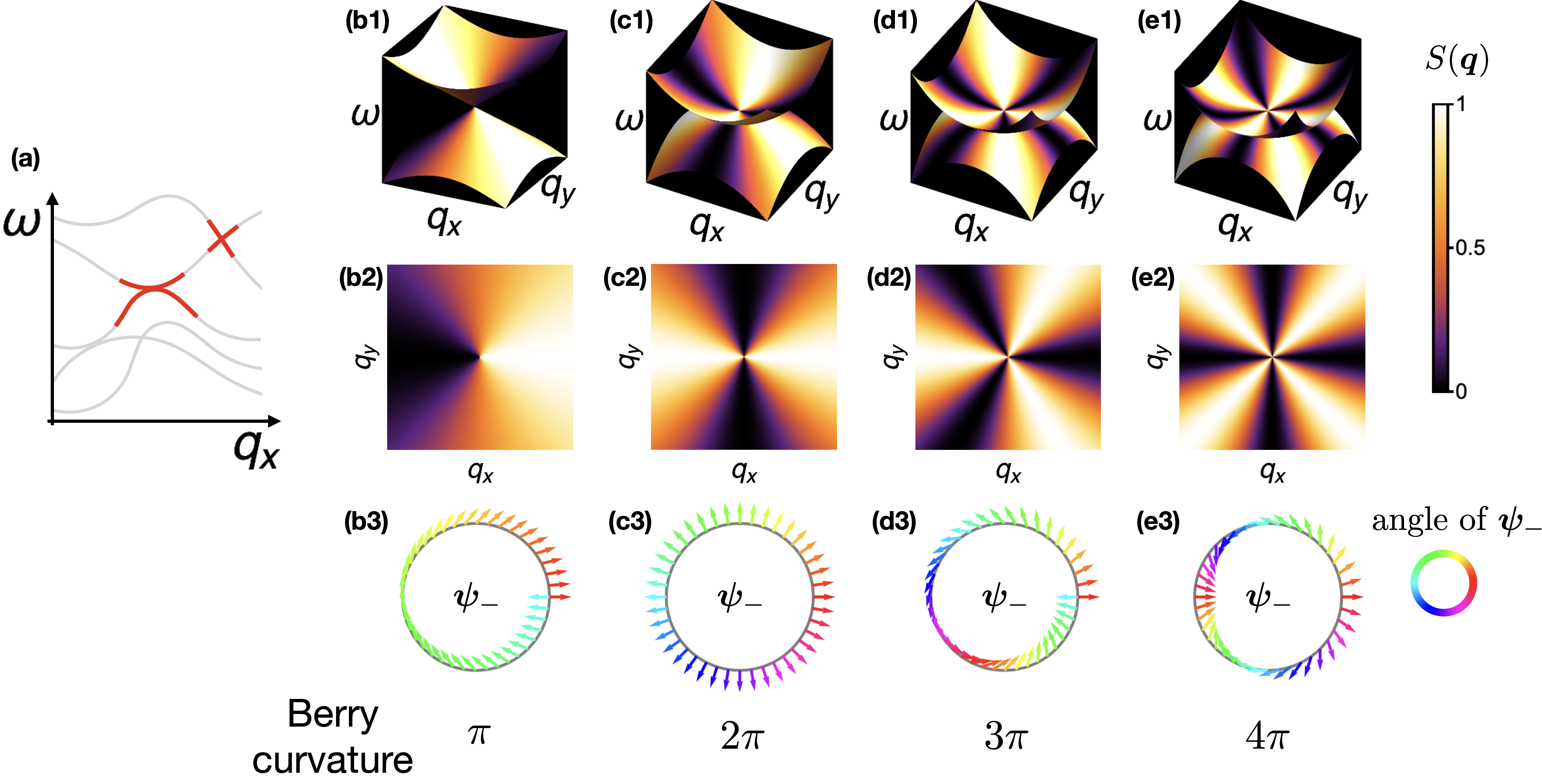
Figure 1: Schematic illustration of $n-$fold pinch points. (a) Band touching scenarios discussed in this paper, highlighted in red. (b-1) 1-fold pinch points imprinted on the two bands. (b-2) the spectroscopy density distribution on the lower band. (b-3) The corresponding configuration of the wavefunction, which winds $\pi$ around the pinch point. It encodes a Berry curvature of $\pm\pi$ at the gapless point. (c,d,e) 2,3,4-fold pinch points illustrated same way as (b).

Experimentalists have actually observed this universal pattern in a various materials [Table. 1], although the hidden connection has not been discussed much. The simplest case, $1-$fold pinch point, is actually a Dirac cone, and has been shown in ARPES experiments [20, 21, 22, 24] on several graphene-based materials [6, 47, 48]. The $2-$fold pinch points appear in bilayer graphene [33], FeSe [41, 42], and various frustrated lattice materials [34, 35, 36, 37, 38, 39, 40, 49, 50, 51, 52, 46, 43] . The $n-$fold pinch point’s implication of the underlying Gauss’s law has been a focus in classical and quantum spin liquids [53, 54, 55, 56, 57, 49, 58, 59, 60, 61, 62], but the connection to Berry curvature has been rarely mentioned.

The universal patterns of pinch points has a high application value. Its advantage relies on the fact that it does not require one to know much about the microscopic details of the matter or to reconstruct the full Hamiltonian. Also, this is particularly useful for two touching-bands with quadratic or higher-order gap-opening dispersion, where the dispersion alone is not a very distinguishing factor like the Dirac cones. Another application is to twisted bilayer systems [63, 64, 65], where the full Hamiltonian for all bands is practically impossible to reconstruct.

Dirac cone as 1-fold pinch point. — We start by introducing the “pinch point”. In this workwe work on 2D systems, but its generalization to 3D is fairly straightforward. The simplest case — $1-$fold pinch point — is imprinted on the most common ingredient of topological band systems: the Weyl/Dirac cone [66, 26, 3].

Consider a local region in the reciprocal momentum space, where two bands have a degenerate point set at $\bm{q}=\bm{0}$ [cf. Fig. 1(a)]. In the neighborhood of $\bm{q}=\bm{0}$, they are also gapped from other bands, so we can focus on the two-band subsystem only.

Spectroscopy measures the band structure as well as the intensity distribution of certain correlation function on each band. We denote the upper and lower band’s dispersion relations as $\omega_{-}(\bm{q})$ and $\omega_{+}(\bm{q})$. The energy and momentum-resolved spectroscopy of the two bands are (assuming infinitely fine resolution)

$$\begin{split}\mathcal{S}_{+}(\omega,\bm{q})=\delta(\omega-\omega_{+}(\bm{q}))S_{+}(\bm{q}),\\ \mathcal{S}_{-}(\omega,\bm{q})=\delta(\omega-\omega_{-}(\bm{q}))S_{-}(\bm{q}).\end{split}$$ (1)

Here, we separated the dispersion $\delta(\omega-\omega_{\pm}(\bm{q}))$ and the intensity distribution $S_{\pm}(\bm{q})$ for future convenience. The intensity $S_{\pm}$ usually measures the amplitude of the wavefunction in a particular basis. For example, in case of graphene, it measures $\braket{(c_{A}^{\dagger}+c_{B}^{\dagger})(c_{A}+c_{B})}$ of the band wavefunction, where $A,B$ are the two sublattice indices, so the basis measured is $c_{A}+c_{B}$. The wavefunction $(1/\sqrt{2},1/\sqrt{2})^{T}$ has maximal intensity, while $(1/\sqrt{2},-1/\sqrt{2})^{T}$ has zero.

The $1-$fold pinch point refers to the spectroscopic intensity $S_{\pm}(\bm{q})$ distribution on the Dirac cone as illustrated in Fig. 1(b2). The intensity distribution only depends on the angle around the gapless point. On one band, it reaches zero on one side, and maximum on the other. The intensity varies smoothly except at the gapless point, where it becomes singular (i.e. not continuous). The other band has a similar pattern of intensity distribution, but the strong and weak regions switch sides. This pattern has in fact been observed in various experiments, as we summarized in Table. 1.

$n-$fold pinch point. — The pattern of $1-$fold pinch point can be generalized to $n-$fold pinch point. The cases of $n=1,2,3,4$ are illustrated in Fig. 1. The upper row panels show the entire energy and momentum resolved spectroscopy, and the mid row panels show the intensity distribution $S_{\pm}(\bm{q})$ without the dispersion.

The crucial ingredient of the $n-$fold pinch point is the singularity in the intensity distribution $S_{\pm}(\bm{q})$. Near $\bm{q}=\bm{0}$, the intensity only depends on the angle $\theta$ around $\bm{0}$. An $n-$fold pinch point has $n$ dark wings where the intensity is low, and $n$ bright wings where the intensity is high. The most symmetric form of the intensity distribution, by choosing a suitable angle as $\theta=0$, is

$$\begin{split}S_{+}(\bm{q})=A\cos^{2}(n\theta/2),\\ S_{-}(\bm{q})=A\sin^{2}(n\theta/2).\end{split}$$ (2)

Here, $A$ is just a scalar signifying the overall intensity. $S_{\pm}(\bm{q})$ at $\bm{q}=\bm{0}$ is singular, since one obtains different values of $S_{\pm}(\bm{0})$ by approaching it from different directions.

For a specific lattice model, the intensity distribution can be mildly distorted up to an isomorphic mapping. The more general form is

$$\begin{split}S_{+}(\bm{q})=A\cos^{2}(n\Theta(\theta)/2),\\ S_{-}(\bm{q})=A\sin^{2}(n\Theta(\theta)/2),\end{split}$$ (3)

where $\Theta(\theta)$ is a smooth, monotonically increasing function as a bijection from $[0,2\pi)$ to itself.

$$\Theta(0)=0,\;\Theta(2\pi)=2\pi,\Theta^{\prime}(\theta)>0.$$ (4)

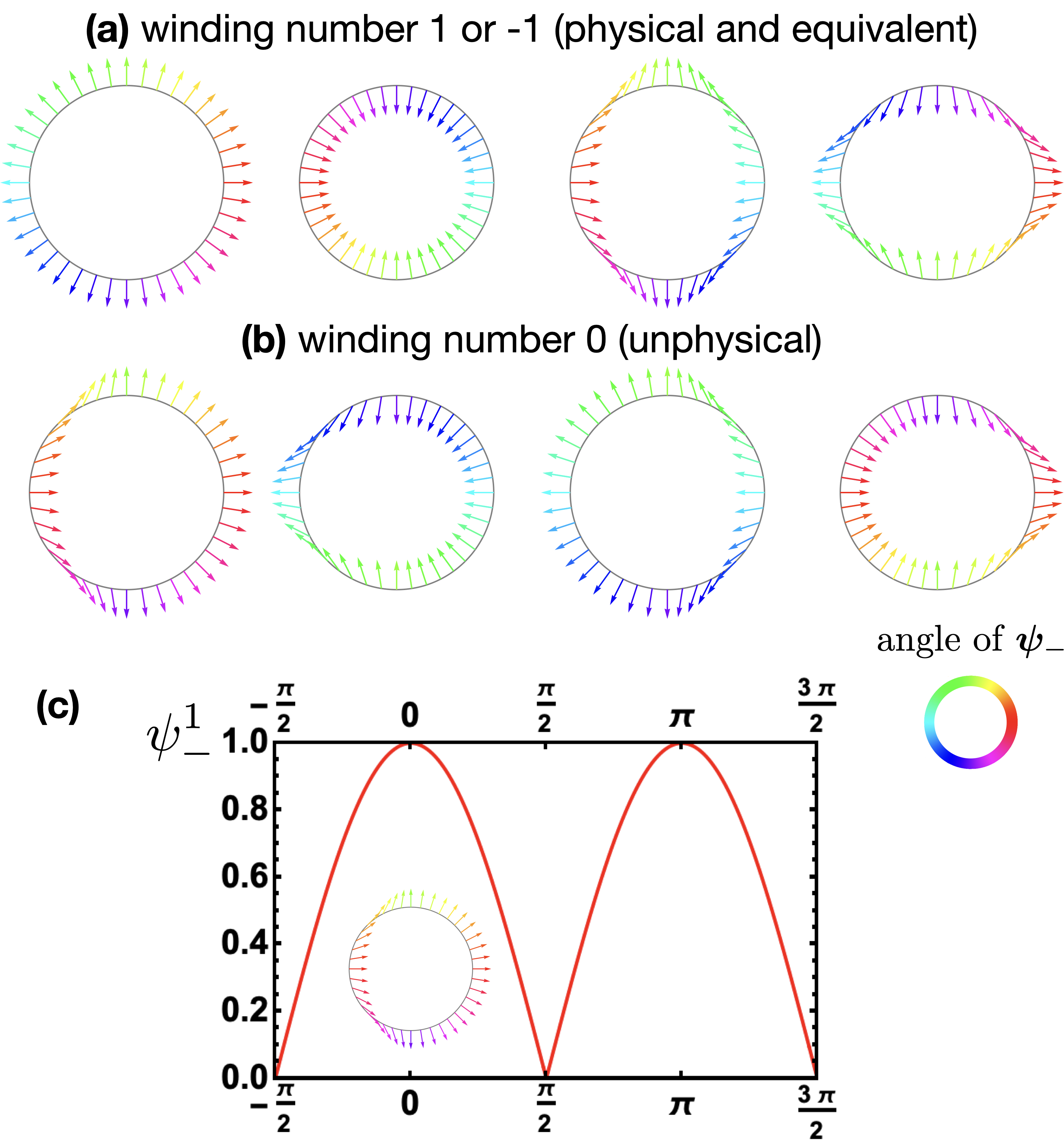
Figure 2: Representative continuous winding configurations of $\bm{\psi}_{-}$ consistent with a 2-fold pinch point. (a) $\bm{\psi}_{-}$ configurations with winding number $\pm 1$, which are also smoothly varying. (b) $\bm{\psi}_{-}$ configurations with winding number $0$, which are not smoothly varying. (c) Plot of $\psi_{-}^{1}$ as a function of angle $\theta$, showing non-smoothness at $\theta=\pi/2,\ 3\pi/2$.

The main message of this paper is that such gapless $n-$fold pinch point is guaranteed to be topologically nontrivial. By “non-trivial” we mean the degenerate point is not accidental, and generally carries a non-zero Berry curvature, except for some extremely fine-tuned cases. A much stronger result is that if the system additionally admits a suitable symmetry (for example, time reversal symmetry for spinless electron systems), then the Berry flux encoded must be $n\pi$.

A remark is in order before we proceed to the proof. In this work we assume that there is no “extrinsic” factors from the coupling between the system and the probing particles (photons or neutrons), which may also exhibit pinch point patterns. For ARPES, if the electron is in an anisotropic orbit, the photon-electron coupling will pick up an angle-dependent projector depending on the polarization of photons, which may yield pinch point patterns. A very detailed discussion can be found in Ref. [67]. One needs to choose the photon polarization (or use unpolarized photons) properly to avoid such effects. The same principle applies to INS – for example, polarized neutrons couple to spin-1/2 dimers in a fixed direction can also have similar projectors. However, these extrinsic, “fake” pinch points are often not present in actual experiment, or at least avoidable in principle. In all examples given in Table. 1, one does not need to worry about them.

Pinch points are topologically critical. — We now prove that under suitable symmetries, the $2-$fold pinch-point singularity is associated with a gapless point with Berry flux $\pm 2\pi$ encoded . Here we take the symmetry be time reversal ($\mathcal{T}$) for the spinless electrons, which forces the Hamiltonian to be real. The proof can be easily generalized to $n-$fold pinch-points and other proper symmetries (see end of section).

The physical picture is the following. The $n-$fold pinch point pattern (Fig. 1(b1-e1)) indicates that the spectroscopy intensity follows a squared-sine function. This requires that the wavefunction of the corresponding band, which is a two component real vector, rotates in a sine/cosine manner on a loop around the gapless point, and accumulate a quantized total rotation angle $n\pi$ (Fig. 1(b3-e3)) at the end. This is exactly the origin of the Berry flux.

Now, onto the formal proof, we first set up the model with a few simplifications without affecting its topological features. In the vicinity of the pinch-point, we consider the relevant subsystem with two degrees of freedom $\psi^{1},\ \psi^{2}$, and their corresponding two-level Hamiltonian. The upper and lower bands correspond to two wavefunctions written as two orthonormal, unit vectors of complex entries

$$\bm{\psi}_{+}(\bm{q})=\begin{pmatrix}\psi_{+}^{1}\\ \psi_{+}^{2}\end{pmatrix},\qquad\bm{\psi}_{-}(\bm{q})=\begin{pmatrix}\psi_{-}^{1}\\ \psi_{-}^{2}\end{pmatrix}.$$ (5)

The system is then described by a Hermitian Hamiltonian

$$\mathcal{H}(\bm{q})=\bm{S}\begin{pmatrix}\omega_{+}(\bm{q})&0\\ 0&\omega_{-}(\bm{q})\end{pmatrix}\bm{S}^{\dagger}.$$ (6)

where $\bm{S}=\left(\bm{\psi}_{+},\bm{\psi}_{-}\right)$ is the eigenvector matrix, and $\omega_{\pm}(\bm{q})$ are the two bands’ dispersion relations.

Under the $\mathcal{T}$ symmetry, the eigenvectors and Hamiltonian are real. Because the spectroscopy intensity follows a squared-sine function, it requires

$$|\psi_{-}^{1}(\bm{q})|\propto|q^{x}|/q=|\sin\theta|.$$ (7)

This puts strong constraint on the possible eigenvector configurations. Some of them are listed in Fig. 2(a,b).

We also require the Hamiltonian to be smooth, i.e., continuous and differentiable to any order. This is generically true for systems with short-rang interactions, and not so only for systems with certain fine-tuned long-range interactions. Hence the requirement applies to most physically realistic systems [68, 69]. It plays a key role in eliminating the physically unrealistic cases shown in Fig. 2(b), because in those cases, the eigenvector has to go though points where unsmooth change of its component(s) is bounded to happen, even though there is no gap closing at those points. One of such unsmooth components is illustrated in Fig. 2(c). A more detailed, technical analysis is presented in the appendix.

Therefore, for $\psi_{-}^{1}$ to vary smoothly, it has to take the form $\psi_{-}^{1}=\sin\theta$ over the entire circle, up to an overall minus sign. After a similar analysis on $\psi_{-}^{2}$ and $\bm{\psi}_{+}$, we can conclude that the viable eigenvectors in $\bm{q}-$space are those in Fig. 2(a), which are all topologically equivalent in eyes of Berry flux at the gapless point. We may pick the eigenvectors to be

$$\begin{split}&\bm{\psi}_{+}(\bm{q})=(-\cos\theta,\sin\theta)=\frac{1}{q}(-q^{y},q^{x}),\\ &\bm{\psi}_{-}(\bm{q})=(\sin\theta,\cos\theta)=\frac{1}{q}(q^{x},q^{y}).\\ \end{split}$$ (8)

The eigenvectors and eigenvalues completely determines the Hamiltonian (cf. Eq (6)). Written as an effective magnetic field coupled to Pauli matrices, it is

$$\begin{split}\mathcal{H}(\bm{q})=&\frac{\omega_{+}(\bm{q})+\omega_{-}(\bm{q})}{2}\mathbb{I}\\ &+\Delta(\bm{q})\frac{(q^{x})^{2}-(q^{y})^{2}}{2q^{2}}\sigma_{z}-\Delta(\bm{q})\frac{q^{x}q^{y}}{q^{2}}\sigma_{x}\\[10.00002pt] \equiv&\frac{\omega_{+}(\bm{q})+\omega_{-}(\bm{q})}{2}\mathbb{I}+\bm{\sigma}\cdot\bm{B}(\bm{q}),\end{split}$$ (9)

where $\Delta(\bm{q})=\omega_{+}(\bm{q})-\omega_{-}(\bm{q})$ is the energy gap.

From the Hamiltonian we can read off the effective magnetic field $\bm{B}(\bm{q})$ to be

$$\bm{B}(\bm{q})=\Delta(\bm{q})\left(-\frac{q^{x}q^{y}}{q^{2}},0,\frac{(q^{x})^{2}-(q^{y})^{2}}{2q^{2}}\right).$$ (10)

The crucial property is that, on a loop around the pinch point, the two components $(B^{x},B^{z})$ as a 2D vector field form a vortex of winding number 2. In Fig. 3(a), the normalized $(B^{x},B^{z},B^{y})/B(\bm{q})$ is plotted. Here we swapped $B^{y}$ and $B^{z}$ for better visualization. This is known to encode a Berry curvature of $\pm 2\pi$ [13]. Another way to see this is to directly compute the Berry flux enclosed by a loop $\bm{q}=q(\cos\theta,\sin\theta)$ around the gapless point, defined as

$$C_{\pm}=\int_{0}^{2\pi}\text{d}\theta\ i\bm{\psi}_{\pm}^{\dagger}\cdot\partial_{\theta}\bm{\psi}_{\pm}.$$ (11)

We conclude our proof here.

This proof can be intuitively generalized to a general $n-$fold pinch point. In Fig. 1, we plot the smoothly varying $\bm{\psi}_{-}$ for different cases. Note that for odd $n$, $\bm{\psi}_{-}$ needs anti-periodic boundary condition instead.

Without the symmetry protection, the different components of an eigenvectors can have different complex phases, so the proof above does not apply any longer, and the Berry-flux at the gapless point is generally not quantized. One example of such scenarios is to add different phases to $\psi^{1}$ and $\psi^{2}$ in Eq. (8), which can yield a finite Berry flux contribution when plugged into Eq. (11), or even render to total Berry zero. In this case, $\bm{B}(\bm{q})/B$ still travels back and forth twice from the north pole to south pole on the unit sphere for a path of $\bm{q}$ around the pinch point. It can be, however, not two great circles, but some general curve. The solid angle enclosed by the path, which is the Berry flux, is then not quantized.

Finally, the picture above also shows that other symmetry protections can also work, if the normalized effective magnetic field is restricted to move on a fixed great circle between the two poles.

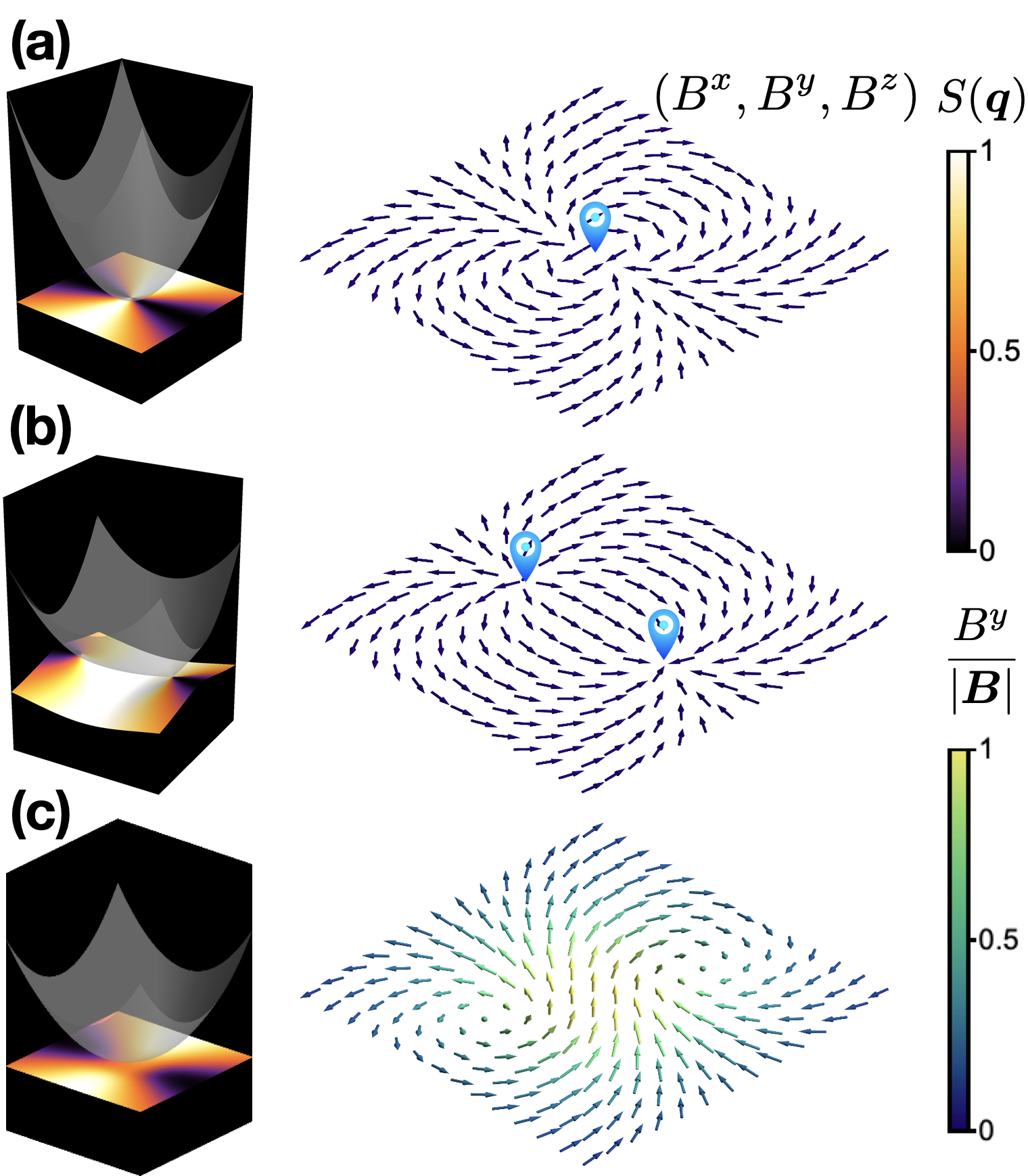
Figure 3: Transformation of 2-fold pinch point and corresponding effective magnetic field configuration. For better visibility we set the upper band to be transparent and focus on the lower band. (a) The 2-fold pinch point and winding number-2 magnetic field in the effective Hamiltonian. (b) Upon introducing $\delta B^{z}$, the gapless point splits into two Dirac points. The 2-fold pinch point splits into two 1-fold pinch point. (c) Upon introducing $\delta B^{y}$, the two bands become gapped and pick up a Chern number. The singularity disappears.

Splitting and gapping the pinch point. — How the topologically critical gapless points transform under different perturbations is a well-studied topic. In this section we revisit some of these transformations, with a focus on the corresponding pinch point phenomenology.

Fig. 3(b) shows a 2-fold pinch point spliting into two 1-fold pinch points (Dirac cones). Correspondingly, the Berry curvature of $2\pi$ is also split into the two 1-fold pinch points each carrying Barry flux $\pi$, assuming the proper symmetry protection. In this process the overall Berry flux is conserved.

Using our model for demonstration, this can be done by introducing a perturbation of constant $B^{z}>0$ for the Hamiltonian in (9), and take $\Delta(\bm{q})=cq^{2}$,

$$\bm{B}_{\text{z-tuned}}(\bm{q})=\left(-cq^{x}q^{y},0,\frac{c}{2}((q^{x})^{2}-(q^{y})^{2})+\delta B^{z}\right).$$ (12)

The original gapless point at $\bm{q}=\bm{0}$ is then split into two linearly dispersive gapless points at $\bm{q}=(0,\pm\sqrt{2\delta B^{z}/c})$. the original winding number-$2$ vortex of $\bm{B}(\bm{q})$ splits into two vortices, each with winding number $1$ [Fig. 3(b)], consistent with the Berry flux conservation.

The critical gapless point can also be gapped, and induces well-defined, opposite non-zero Berry curvature on the two bands locally. We can consider perturbing the effective magnetic field in the following way,

$$\bm{B}_{\text{y-tuned}}(\bm{q})=\left(-cq^{x}q^{y},\delta B^{y},\frac{c}{2}((q^{x})^{2}-(q^{y})^{2})\right).$$ (13)

As a consequence, the normalized $\bm{B}_{\text{y-tuned}}/B_{\text{y-tuned}}$ form half a skyrmion, or a meron, as illustrated in Fig. 3(c). Since the skyrmion is of winding number $2$, the two bands get local Berry curvature $\pm 2\pi$. The $\pm$ sign depends on the sign of $\delta B^{y}$, and cannot be distinguished from the spectroscopy pattern.

The pinch point singularity disappears as the gap opens. The spectroscopic intensity on two bands becomes smooth at the center, but gradually recovers the pinch point pattern when zoomed out. An example of this will be discussed in detail in a separate work studying the Kagome model [70]. Similar examples can also be found in Refs. [71, 72].

Discussion. — The main message of this work is that the $n-$fold pinch points observed in energy-momentum resolved spectroscopy indicate that the gapless point is topologically critical, and encodes Berry flux $n\pi$ if there is a suitable symmetry protection. We have proven this for time reversal symmetry, and also provided a survey of experiments (Table. 1) that observe the universal phenomenon. This result does not rely on further microscopic details of the system, hence has great potential in experimental application across several platforms including ARPES, STM, and INS.

Another useful lesson is that the reversed conclusion is often but not always true: a topologically critical gapless point may appear as a $n-$fold pinch point. Some of these cases has been discussed in Refs. [26, 73, 66], although the connection to pinch points were not mentioned. It is not always true, because the winding of certain wavefunction may not be captured by the correlation function measured by spectroscopy. The Honeycomb and Kagome lattice magnon models studied in Ref. [74, 75, 58] are such examples, in which some critical gapless points appear as 1FPP and 2FPP, but some are completely dark in the structure factor due to extrinsic, accidental cancellation of form factor.

The bigger picture we gain from this work is that the spectroscopy contains a huge amount of information, of which a lot are still waiting to be exploited. For example, instead of points, other topologically critical loci of band degeneracy should also manifest universal, characteristic patterns. This idea also applies to interacting or non-Hermitian Hamiltonians. Developing the zoology of them will be an important and useful piece of phenomenological study.

In this section, we give a detailed proof of Eq. (8). That is, the squared-sin pattern of the spectra distribution indicates that the corresponding eigenvector has to be equivalent to Eq. (8), or those Fig. 2(a). The configurations in Fig. 2(b) are forbidden.

To start with, we have the freedom to choose the basis $(1,0)$ to be the one on which the spectroscopy measures the amplitude of the wavefunction. This is because the spectroscopy is measuring the expectation value of certain operator of scalar degree of freedom. So we have

$$\begin{split}S_{+}(\bm{q})\propto|(1,0)\cdot(\psi^{1}_{+},\psi^{2}_{+})^{\mathrm{T}}(\bm{q})|^{2}=|\psi_{+}^{1}(\bm{q})|^{2},\\ S_{-}(\bm{q})\propto|(1,0)\cdot(\psi^{1}_{-},\psi^{2}_{-})^{\mathrm{T}}(\bm{q})|^{2}=|\psi_{-}^{1}(\bm{q})|^{2}.\end{split}$$ (S1)

In the example of graphene, $\psi^{1}\sim c_{A}+c_{B}$ is measured by ARPES, and $\psi^{2}\sim c_{A}-c_{B}$. We also assume that the pinch point pattern is in its most symmetric form

$$\begin{split}S_{+}(\bm{q})=A\cos^{2}(\theta)=A\frac{(q^{y})^{2}}{q^{2}},\\ S_{-}(\bm{q})=A\sin^{2}(\theta)=A\frac{(q^{x})^{2}}{q^{2}}.\end{split}$$ (S2)

A small distortion of the pinch point in form of Eq. (3) does not affect our conclusions on its topological features.

Combining Eq. (S1) and Eq. (S2), we see that

$$|\psi_{-}^{1}(\bm{q})|\propto|q^{x}|/q=|\sin\theta|.$$ (S3)

Since $\bm{\psi}_{-}$ is a unit vector, we then also know

$$|\psi_{-}^{2}(\bm{q})|\propto|q^{y}|/q=|\cos\theta|,$$ (S4)

There are several ways to arrange continuously varying $\bm{\psi_{-}}$ on a circle around the pinch point and satisfy conditions of Eq. (S3) and Eq. (S4). Some representatives are illustrated in Fig. 2(a,b).

The configurations in the same row are physically identical, since they can be related to each other by introducing minus signs to the basis $\psi^{1}$ or $\psi^{2}$. The configurations in Fig. 2(a), compared to those in Fig. 2(b), are physically different: the first row has winding number $\pm 1$, and the second has winding number $0$.

A key observation is that $\psi_{-}^{1}$ configurations with zero winding number are not smooth, hence do not yield a smooth Hamiltonian. Taking the first case of Fig. 2(b) as an example, $\psi_{-}^{1}$ takes a sharp turn at $\theta=\pm\pi/2$ as shown in the Fig. 2(c). However, $\psi_{-}^{2}=\pm 1$, and varies smoothly following a sine curve at these two point. The Hamiltonian is

$$\mathcal{H}(\bm{q})=\bm{S}\begin{pmatrix}\omega_{+}(\bm{q})&0\\ 0&\omega_{-}(\bm{q})\end{pmatrix}\bm{S}^{\dagger}.$$ (S5)

where $\bm{S}=\left(\bm{\psi}_{+},\bm{\psi}_{-}\right)$. So its off-diagonal terms component, containing $\omega_{-}\psi_{-}^{1}\psi_{-}^{2}$, is then not smooth.

One may want to amend this problem by “softening” the sharp turn of $\psi_{-}^{1}$ at $\theta=\pi/2,\ 3\pi/2$, hoping that it will yield a distorted pinch point described by some function $\Theta(\theta)$ in Eq. (3) and has a smooth Hamiltonian. However, in this case we always have $\psi_{-}^{1\prime}=\psi_{-}^{2\prime}=0$, so that $\Theta^{\prime}(\theta_{0})=0$ at the points $\Theta(\theta_{0})=\pi/2,\ 3\pi/2$, which is not the proper pinch point pattern defined in Eq. (4) anymore. Such unauthentic pinch points can be distinguished in experiments since $\Theta(\theta)$ can be measured.

Therefore, the eigenvector configurations in Fig. 2(b) are forbidden. It has to be equivalent to Eq. (8), or those Fig. 2(a), which encodes a Berry flux at the gapless point as shown in the main text.

References

- Hasan and Kane [2010] M. Z. Hasan and C. L. Kane, Colloquium: Topological insulators, Rev. Mod. Phys. 82, 3045 (2010).
- Qi and Zhang [2011] X.-L. Qi and S.-C. Zhang, Topological insulators and superconductors, Rev. Mod. Phys. 83, 1057 (2011).
- McClarty [2022] P. A. McClarty, Topological magnons: A review, Annual Review of Condensed Matter Physics 13, 171 (2022), https://doi.org/10.1146/annurev-conmatphys-031620-104715 .
- Bansil et al. [2016] A. Bansil, H. Lin, and T. Das, Colloquium: Topological band theory, Rev. Mod. Phys. 88, 021004 (2016).
- Haldane [1988] F. D. M. Haldane, Model for a quantum hall effect without landau levels: Condensed-matter realization of the ”parity anomaly”, Phys. Rev. Lett. 61, 2015 (1988).
- Kane and Mele [2005a] C. L. Kane and E. J. Mele, Quantum spin hall effect in graphene, Phys. Rev. Lett. 95, 226801 (2005a).
- Kane and Mele [2005b] C. L. Kane and E. J. Mele, topological order and the quantum spin hall effect, Phys. Rev. Lett. 95, 146802 (2005b).
- Fu et al. [2007] L. Fu, C. L. Kane, and E. J. Mele, Topological insulators in three dimensions, Phys. Rev. Lett. 98, 106803 (2007).
- Moore and Balents [2007] J. E. Moore and L. Balents, Topological invariants of time-reversal-invariant band structures, Phys. Rev. B 75, 121306 (2007).
- Roy [2009] R. Roy, Topological phases and the quantum spin hall effect in three dimensions, Phys. Rev. B 79, 195322 (2009).
- Bernevig et al. [2006] B. A. Bernevig, T. L. Hughes, and S.-C. Zhang, Quantum spin hall effect and topological phase transition in HgTe quantum wells, Science 314, 1757 (2006).
- Katsura et al. [2010] H. Katsura, N. Nagaosa, and P. A. Lee, Theory of the thermal hall effect in quantum magnets, Phys. Rev. Lett. 104, 066403 (2010).
- Bernevig and Hughes [2013] B. A. Bernevig and T. L. Hughes, Topological Insulators and Topological Superconductors (Princeton University Press, 2013).
- Damascelli et al. [2003] A. Damascelli, Z. Hussain, and Z.-X. Shen, Angle-resolved photoemission studies of the cuprate superconductors, Rev. Mod. Phys. 75, 473 (2003).
- Binnig and Rohrer [1987] G. Binnig and H. Rohrer, Scanning tunneling microscopy—from birth to adolescence, Rev. Mod. Phys. 59, 615 (1987).
- Fischer et al. [2007] O. Fischer, M. Kugler, I. Maggio-Aprile, C. Berthod, and C. Renner, Scanning tunneling spectroscopy of high-temperature superconductors, Rev. Mod. Phys. 79, 353 (2007).
- Squires [2012] G. L. Squires, Introduction to the Theory of Thermal Neutron Scattering (Cambridge University Press, 2012).
- Milićević et al. [2019] M. Milićević, G. Montambaux, T. Ozawa, O. Jamadi, B. Real, I. Sagnes, A. Lemaître, L. Le Gratiet, A. Harouri, J. Bloch, and A. Amo, Type-iii and tilted dirac cones emerging from flat bands in photonic orbital graphene, Phys. Rev. X 9, 031010 (2019).
- Harris et al. [1997] M. J. Harris, S. T. Bramwell, D. F. McMorrow, T. Zeiske, and K. W. Godfrey, Geometrical frustration in the ferromagnetic pyrochlore , Phys. Rev. Lett. 79, 2554 (1997).
- Bostwick et al. [2006] A. Bostwick, T. Ohta, T. Seyller, K. Horn, and E. Rotenberg, Quasiparticle dynamics in graphene, Nature Physics 3, 36 (2006).
- Fedorov et al. [2014] A. V. Fedorov, N. I. Verbitskiy, D. Haberer, C. Struzzi, L. Petaccia, D. Usachov, O. Y. Vilkov, D. V. Vyalikh, J. Fink, M. Knupfer, B. Büchner, and A. Grüneis, Observation of a universal donor-dependent vibrational mode in graphene, Nature Communications 5, 10.1038/ncomms4257 (2014).
- Ludbrook et al. [2015] B. M. Ludbrook, G. Levy, P. Nigge, M. Zonno, M. Schneider, D. J. Dvorak, C. N. Veenstra, S. Zhdanovich, D. Wong, P. Dosanjh, C. Straßer, A. Stöhr, S. Forti, C. R. Ast, U. Starke, and A. Damascelli, Evidence for superconductivity in li-decorated monolayer graphene, Proceedings of the National Academy of Sciences 112, 11795 (2015).
- Cheng et al. [2015] C.-M. Cheng, L. Xie, A. Pachoud, H. Moser, W. Chen, A. Wee, A. C. Neto, K.-D. Tsuei, and B. Özyilmaz, Anomalous spectral features of a neutral bilayer graphene, Scientific Reports 5, 10.1038/srep10025 (2015).
- Ahn et al. [2018] S. J. Ahn, P. Moon, T.-H. Kim, H.-W. Kim, H.-C. Shin, E. H. Kim, H. W. Cha, S.-J. Kahng, P. Kim, M. Koshino, Y.-W. Son, C.-W. Yang, and J. R. Ahn, Dirac electrons in a dodecagonal graphene quasicrystal, Science 361, 782 (2018).
- Yuan et al. [2020] B. Yuan, I. Khait, G.-J. Shu, F. C. Chou, M. B. Stone, J. P. Clancy, A. Paramekanti, and Y.-J. Kim, Dirac magnons in a honeycomb lattice quantum magnet , Phys. Rev. X 10, 011062 (2020).
- Elliot et al. [2021] M. Elliot, P. A. McClarty, D. Prabhakaran, R. D. Johnson, H. C. Walker, P. Manuel, and R. Coldea, Order-by-disorder from bond-dependent exchange and intensity signature of nodal quasiparticles in a honeycomb cobaltate, Nature Communications 12, 10.1038/s41467-021-23851-0 (2021).
- Zhang et al. [2020] H. Zhang, X. Feng, T. Heitmann, A. I. Kolesnikov, M. B. Stone, Y.-M. Lu, and X. Ke, Topological magnon bands in a room-temperature kagome magnet, Phys. Rev. B 101, 100405 (2020).
- Chen et al. [2018] L. Chen, J.-H. Chung, B. Gao, T. Chen, M. B. Stone, A. I. Kolesnikov, Q. Huang, and P. Dai, Topological spin excitations in honeycomb ferromagnet , Phys. Rev. X 8, 041028 (2018).
- Chen et al. [2021] L. Chen, J.-H. Chung, M. B. Stone, A. I. Kolesnikov, B. Winn, V. O. Garlea, D. L. Abernathy, B. Gao, M. Augustin, E. J. G. Santos, and P. Dai, Magnetic field effect on topological spin excitations in , Phys. Rev. X 11, 031047 (2021).
- Cai et al. [2021] Z. Cai, S. Bao, Z.-L. Gu, Y.-P. Gao, Z. Ma, Y. Shangguan, W. Si, Z.-Y. Dong, W. Wang, Y. Wu, D. Lin, J. Wang, K. Ran, S. Li, D. Adroja, X. Xi, S.-L. Yu, X. Wu, J.-X. Li, and J. Wen, Topological magnon insulator spin excitations in the two-dimensional ferromagnet , Phys. Rev. B 104, L020402 (2021).
- Zhu et al. [2021] F. Zhu, L. Zhang, X. Wang, F. J. dos Santos, J. Song, T. Mueller, K. Schmalzl, W. F. Schmidt, A. Ivanov, J. T. Park, J. Xu, J. Ma, S. Lounis, S. Blügel, Y. Mokrousov, Y. Su, and T. Brückel, Topological magnon insulators in two-dimensional van der waals ferromagnets and : Toward intrinsic gap-tunability, Science Advances 7, 10.1126/sciadv.abi7532 (2021).
- Ye et al. [2018] L. Ye, M. Kang, J. Liu, F. Von Cube, C. R. Wicker, T. Suzuki, C. Jozwiak, A. Bostwick, E. Rotenberg, D. C. Bell, et al., Massive dirac fermions in a ferromagnetic kagome metal, Nature 555, 638 (2018).
- Joucken et al. [2020] F. Joucken, Z. Ge, E. A. Quezada-López, J. L. Davenport, K. Watanabe, T. Taniguchi, and J. Velasco, Determination of the trigonal warping orientation in bernal-stacked bilayer graphene via scanning tunneling microscopy, Phys. Rev. B 101, 161103 (2020).
- Petit et al. [2016] S. Petit, E. Lhotel, B. Canals, M. C. Hatnean, J. Ollivier, H. Mutka, E. Ressouche, A. R. Wildes, M. R. Lees, and G. Balakrishnan, Observation of magnetic fragmentation in spin ice, Nature Physics 12, 746 (2016).
- Lhotel et al. [2018] E. Lhotel, S. Petit, M. C. Hatnean, J. Ollivier, H. Mutka, E. Ressouche, M. R. Lees, and G. Balakrishnan, Evidence for dynamic kagome ice, Nature Communications 9, 10.1038/s41467-018-06212-2 (2018).
- Xu et al. [2020] J. Xu, O. Benton, A. T. M. N. Islam, T. Guidi, G. Ehlers, and B. Lake, Order out of a coulomb phase and higgs transition: Frustrated transverse interactions of , Phys. Rev. Lett. 124, 097203 (2020).
- Xu et al. [2019] J. Xu, O. Benton, V. K. Anand, A. T. M. N. Islam, T. Guidi, G. Ehlers, E. Feng, Y. Su, A. Sakai, P. Gegenwart, and B. Lake, Anisotropic exchange hamiltonian, magnetic phase diagram, and domain inversion of , Phys. Rev. B 99, 144420 (2019).
- Balz et al. [2016] C. Balz, B. Lake, J. Reuther, H. Luetkens, R. Schonemann, T. Herrmannsdorfer, Y. Singh, A. T. M. Nazmul Islam, E. M. Wheeler, J. A. Rodriguez-Rivera, T. Guidi, G. G. Simeoni, C. Baines, and H. Ryll, Physical realization of a quantum spin liquid based on a complex frustration mechanism, Nat. Phys. 12, 942 (2016).
- Balz et al. [2017a] C. Balz, B. Lake, A. T. M. Nazmul Islam, Y. Singh, J. A. Rodriguez-Rivera, T. Guidi, E. M. Wheeler, G. G. Simeoni, and H. Ryll, Magnetic Hamiltonian and phase diagram of the quantum spin liquid , Phys. Rev. B 95, 174414 (2017a).
- Balz et al. [2017b] C. Balz, B. Lake, M. Reehuis, A. T. M. N. Islam, O. Prokhnenko, Y. Singh, P. Pattison, and S. Tóth, Crystal growth, structure and magnetic properties of Ca10Cr7O28, Journal of Physics: Condensed Matter 29, 225802 (2017b).
- Liu et al. [2012] D. Liu, W. Zhang, D. Mou, J. He, Y.-B. Ou, Q.-Y. Wang, Z. Li, L. Wang, L. Zhao, S. He, Y. Peng, X. Liu, C. Chen, L. Yu, G. Liu, X. Dong, J. Zhang, C. Chen, Z. Xu, J. Hu, X. Chen, X. Ma, Q. Xue, and X. Zhou, Electronic origin of high-temperature superconductivity in single-layer FeSe superconductor, Nature Communications 3, 10.1038/ncomms1946 (2012).
- Wang et al. [2016] Z. F. Wang, H. Zhang, D. Liu, C. Liu, C. Tang, C. Song, Y. Zhong, J. Peng, F. Li, C. Nie, L. Wang, X. J. Zhou, X. Ma, Q. K. Xue, and F. Liu, Topological edge states in a high-temperature superconductor FeSe/SrTiO3(001) film, Nature Materials 15, 968 (2016).
- Kang et al. [2020] M. Kang, S. Fang, L. Ye, H. C. Po, J. Denlinger, C. Jozwiak, A. Bostwick, E. Rotenberg, E. Kaxiras, J. G. Checkelsky, and R. Comin, Topological flat bands in frustrated kagome lattice CoSn, Nature Communications 11, 10.1038/s41467-020-17465-1 (2020).
- Liu et al. [2020] Z. Liu, M. Li, Q. Wang, G. Wang, C. Wen, K. Jiang, X. Lu, S. Yan, Y. Huang, D. Shen, J.-X. Yin, Z. Wang, Z. Yin, H. Lei, and S. Wang, Orbital-selective dirac fermions and extremely flat bands in frustrated kagome-lattice metal CoSn, Nature Communications 11, 10.1038/s41467-020-17462-4 (2020).
- Mena et al. [2014] M. Mena, R. S. Perry, T. G. Perring, M. D. Le, S. Guerrero, M. Storni, D. T. Adroja, C. Rüegg, and D. F. McMorrow, Spin-wave spectrum of the quantum ferromagnet on the pyrochlore lattice , Phys. Rev. Lett. 113, 047202 (2014).
- Chisnell et al. [2015] R. Chisnell, J. S. Helton, D. E. Freedman, D. K. Singh, R. I. Bewley, D. G. Nocera, and Y. S. Lee, Topological magnon bands in a kagome lattice ferromagnet, Phys. Rev. Lett. 115, 147201 (2015).
- Novoselov et al. [2005] K. S. Novoselov, A. K. Geim, S. V. Morozov, D. Jiang, M. I. Katsnelson, I. V. Grigorieva, S. V. Dubonos, and A. A. Firsov, Two-dimensional gas of massless dirac fermions in graphene, Nature 438, 197 (2005).
- Zhang et al. [2005] Y. Zhang, Y.-W. Tan, H. L. Stormer, and P. Kim, Experimental observation of the quantum hall effect and berry's phase in graphene, Nature 438, 201 (2005).
- Benton [2016] O. Benton, Quantum origins of moment fragmentation in , Phys. Rev. B 94, 104430 (2016).
- Kshetrimayum et al. [2020] A. Kshetrimayum, C. Balz, B. Lake, and J. Eisert, Tensor network investigation of the double layer kagome compound ca10cr7o28, Annals of Physics 421, 168292 (2020).
- Sonnenschein et al. [2019] J. Sonnenschein, C. Balz, U. Tutsch, M. Lang, H. Ryll, J. A. Rodriguez-Rivera, A. T. M. N. Islam, B. Lake, and J. Reuther, Signatures for spinons in the quantum spin liquid candidate , Phys. Rev. B 100, 174428 (2019).
- Pohle et al. [2021] R. Pohle, H. Yan, and N. Shannon, Theory of ca10cr7o28 as a bilayer breathing-kagome magnet: Classical thermodynamics and semi-classical dynamics (2021), arXiv:2103.08790 [cond-mat.str-el] .
- Moessner and Chalker [1998] R. Moessner and J. T. Chalker, Low-temperature properties of classical geometrically frustrated antiferromagnets, Phys. Rev. B 58, 12049 (1998).
- Huse et al. [2003] D. A. Huse, W. Krauth, R. Moessner, and S. L. Sondhi, Coulomb and liquid dimer models in three dimensions, Phys. Rev. Lett. 91, 167004 (2003).
- Henley [2010] C. L. Henley, The “coulomb phase” in frustrated systems, Annual Review of Condensed Matter Physics 1, 179 (2010).
- Benton et al. [2016] O. Benton, L. Jaubert, H. Yan, and N. Shannon, A spin-liquid with pinch-line singularities on the pyrochlore lattice, Nature Communications 7, 10.1038/ncomms11572 (2016).
- Prem et al. [2018] A. Prem, S. Vijay, Y.-Z. Chou, M. Pretko, and R. M. Nandkishore, Pinch point singularities of tensor spin liquids, Phys. Rev. B 98, 165140 (2018).
- Yan et al. [2018] H. Yan, R. Pohle, and N. Shannon, Half moons are pinch points with dispersion, Phys. Rev. B 98, 140402 (2018).
- Yan et al. [2020] H. Yan, O. Benton, L. D. C. Jaubert, and N. Shannon, Rank–2 spin liquid on the breathing pyrochlore lattice, Phys. Rev. Lett. 124, 127203 (2020).
- Yan and Nevidomskyy [2022] H. Yan and A. H. Nevidomskyy, Phonon induced rank-2 u(1) nematic liquid states (2022), arXiv:2108.11484 [cond-mat.str-el] .
- Yan and Reuther [2022] H. Yan and J. Reuther, Low-energy structure of spiral spin liquids, Phys. Rev. Res. 4, 023175 (2022).
- Benton and Moessner [2021] O. Benton and R. Moessner, Topological route to new and unusual coulomb spin liquids, Phys. Rev. Lett. 127, 107202 (2021).
- Cao et al. [2018a] Y. Cao, V. Fatemi, A. Demir, S. Fang, S. L. Tomarken, J. Y. Luo, J. D. Sanchez-Yamagishi, K. Watanabe, T. Taniguchi, E. Kaxiras, R. C. Ashoori, and P. Jarillo-Herrero, Correlated insulator behaviour at half-filling in magic-angle graphene superlattices, Nature 556, 80 (2018a).
- Cao et al. [2018b] Y. Cao, V. Fatemi, S. Fang, K. Watanabe, T. Taniguchi, E. Kaxiras, and P. Jarillo-Herrero, Unconventional superconductivity in magic-angle graphene superlattices, Nature 556, 43 (2018b).
- Lisi et al. [2020] S. Lisi, X. Lu, T. Benschop, T. A. de Jong, P. Stepanov, J. R. Duran, F. Margot, I. Cucchi, E. Cappelli, A. Hunter, A. Tamai, V. Kandyba, A. Giampietri, A. Barinov, J. Jobst, V. Stalman, M. Leeuwenhoek, K. Watanabe, T. Taniguchi, L. Rademaker, S. J. van der Molen, M. P. Allan, D. K. Efetov, and F. Baumberger, Observation of flat bands in twisted bilayer graphene, Nature Physics 17, 189 (2020).
- Shivam et al. [2017] S. Shivam, R. Coldea, R. Moessner, and P. McClarty, Neutron scattering signatures of magnon weyl points (2017), arXiv:1712.08535 [cond-mat.str-el] .
- Moser [2017] S. Moser, An experimentalist's guide to the matrix element in angle resolved photoemission, Journal of Electron Spectroscopy and Related Phenomena 214, 29 (2017).
- Bloch [1929] F. Bloch, Über die Quantenmechanik der Elektronen in Kristallgittern, Zeitschrift fur Physik 52, 555 (1929).
- Bouckaert et al. [1936] L. P. Bouckaert, R. Smoluchowski, and E. Wigner, Theory of brillouin zones and symmetry properties of wave functions in crystals, Phys. Rev. 50, 58 (1936).
- Yan et al. [2023] H. Yan, A. Thomasen, J. Romhányi, and N. Shannon, Pinch points and half moons encode berry curvature (2023), arXiv:2304.02203 [cond-mat.str-el] .
- Sun et al. [2009] K. Sun, H. Yao, E. Fradkin, and S. A. Kivelson, Topological insulators and nematic phases from spontaneous symmetry breaking in 2d fermi systems with a quadratic band crossing, Phys. Rev. Lett. 103, 046811 (2009).
- Sun and Fradkin [2008] K. Sun and E. Fradkin, Time-reversal symmetry breaking and spontaneous anomalous hall effect in fermi fluids, Phys. Rev. B 78, 245122 (2008).
- Mucha-Kruczyński et al. [2008] M. Mucha-Kruczyński, O. Tsyplyatyev, A. Grishin, E. McCann, V. I. Fal’ko, A. Bostwick, and E. Rotenberg, Characterization of graphene through anisotropy of constant-energy maps in angle-resolved photoemission, Phys. Rev. B 77, 195403 (2008).
- Maksimov and Chernyshev [2016] P. A. Maksimov and A. L. Chernyshev, Field-induced dynamical properties of the model on a honeycomb lattice, Phys. Rev. B 93, 014418 (2016).
- Chernyshev and Zhitomirsky [2015] A. L. Chernyshev and M. E. Zhitomirsky, Order and excitations in kagome-lattice antiferromagnets, Phys. Rev. B 92, 144415 (2015).
Appendix for “Identifying topologically critical band from pinch-point singularities in spectroscopy”