MP-FedCL: Multiprototype Federated Contrastive Learning for Edge Intelligence
Abstract
Federated learning-assisted edge intelligence enables privacy protection in modern intelligent services. However, not independent and identically distributed (non-IID) distribution among edge clients can impair the local model performance. The existing single prototype-based strategy represents a class by using the mean of the feature space. However, feature spaces are usually not clustered, and a single prototype may not represent a class well. Motivated by this, this paper proposes a multi-prototype federated contrastive learning approach (MP-FedCL) which demonstrates the effectiveness of using a multi-prototype strategy over a single-prototype under non-IID settings, including both label and feature skewness. Specifically, a multi-prototype computation strategy based on k-means is first proposed to capture different embedding representations for each class space, using multiple prototypes ( centroids) to represent a class in the embedding space. In each global round, the computed multiple prototypes and their respective model parameters are sent to the edge server for aggregation into a global prototype pool, which is then sent back to all clients to guide their local training. Finally, local training for each client minimizes their own supervised learning tasks and learns from shared prototypes in the global prototype pool through supervised contrastive learning, which encourages them to learn knowledge related to their own class from others and reduces the absorption of unrelated knowledge in each global iteration. Experimental results on MNIST, Digit-5, Office-10, and DomainNet show that our method outperforms multiple baselines, with an average test accuracy improvement of about 4.6% and 10.4% under feature and label non-IID distributions, respectively.
Index Terms:
Federated learning, edge intelligence, contrastive learning, multi-prototype, global prototype pool, label and feature non-IID, communication efficiency.I Introduction
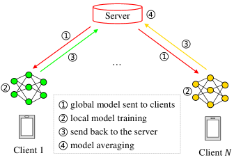
Increasingly, intelligence devices in distributed networks are showing explosive growth, which generates a huge amount of raw data that needs to be processed [1]. Because of the challenges of limitation in network bandwidth or the requirements for transmission delay, the traditional cloud computing paradigm that uploads such big data to a cloud centre for data processing can no longer meet these demands [2]. Thanks to the improvements in storage and computing capabilities of edge intelligence devices, most computing tasks can now be completed directly at the edge, making the mobile edge computing (MEC) paradigm the next-generation computing network [3]. Further, collecting data from distributed devices poses risks and challenges due to the sensitive nature of a large amount of data, as well as regulations such as the general data protection regulation (GDPR) [4] in Europe. Therefore, as edge devices’ storage and computing power continue to grow, coupled with concerns about privacy issues, it becomes more attractive to implement edge intelligence in MEC systems in a distributed manner [5]. To this end, federated learning (FL), as one application of edge computing in distributed machine learning, is first proposed by [6] to simultaneously achieve edge intelligence and address privacy concerns. It trains a global model through the cooperation between local clients and an edge server while keeping the clients’ raw data within their respective local environments. In general, the typical federated training process consists of the following four steps [6]: (1) the server chooses a certain network architecture such as convolutional neural network (CNN) as the global model to be optimized and sends it to local clients; (2) the clients update the received the model parameters of the global model based on their local data; (3) all clients send their updated model parameters back to the edge server for aggregation; (4) the server averages all the sent parameters as the new global model parameters for the next global round, repeating these four steps until convergence. In this fashion, FL’s ability to protect data confidentiality and enable multiple parties to cooperatively train a model makes it a highly promising technology for the future of network intelligence[7].
Nonetheless, a main challenge in FL is that data distribution among clients is usually not independent and identically distributed (non-IID), which can result in reduced effectiveness of FL [8, 9]. To tackle the issue, existing research works under non-IID scenarios can be mainly divided into two categories in terms of optimization objectives, i.e., typical FL [6, 10, 11, 12] and personalized FL [9, 13, 14, 15, 16]. The former objective is to develop a single shared global model that is accurate and efficient, while also capable of adapting to the unique characteristics of each client’s data. FedAvg [6] is the first FL optimization algorithm to enable efficient training of machine learning models on decentralized data. It achieves this through collaborative training of a shared global model via model parameter transmission among clients in each global round. FedLC [10] adopts a fine-grained calibration strategy for clients’ cross-entropy loss to mitigate the bias caused by label distribution skewness among clients in the global model. However, training the global model directly with heterogeneous data from local clients can result in poor generalization abilities to unseen data [17]. In contrast, the latter approach focuses on optimizing local models individually for each client rather than using a shared global model. This is typically achieved by adding a regularization term to the local objective of each client to guide their local training, which enables the models to generalize well to new data. FedProx [9] proposes to add a local regularization term in the local objective of each client to correct the bias between local models and the global model. PFedMe [13] proposes to add an additional term to allow clients to update their local models in different directions without deviating from a global reference point. FedPer [15] proposes a strategy of adding a personalized layer to the base layer and suggests updating only the base layer during the federated training process. Afterwards, clients can update their personalized layer based on their own local data. Additionally, [18] explores a benchmark for non-IID settings, they divide non-IID settings into five cases, such as label distribution skew, feature distribution skew, quantity skew, etc. Further, as [18] mentioned, some existing studies [9, 10, 11, 19] cover only one non-IID case, which do not give sufficient evaluations to this challenge. Therefore, to avoid the influence of biased global models and to evaluate non-IID cases as comprehensively as possible, we focus on personalized FL by optimizing the local objective of each local client under the label and feature distribution skewness.
Inspired by prototypical networks [22], which adopts a single prototype to represent each class by calculating the mean of the class’s embedding space. This prototype can serve as an important information carrier to boost the performance of various learning domains, and has been successfully applied in meta-learning [23], multi-task learning [24], and transfer learning [25]. There have been some existing works [19, 26, 27, 28] introducing the concept of prototypes into FL. FedProto [19] proposes to reduce communication overhead by only exchanging prototypes between clients and the server, instead of exchanging gradients or model parameters. FedPCL [27] proposes to use multiple pre-trained models to extract the features separately, and then they use a projection network to fuse these extracted features in a personalized way while keeping the shared representation compact for efficient communication. These works adopt a single prototype to represent each class and argue that directly averaging the representations from heterogeneous data across clients can effectively capture the embedding representations of each class.
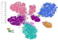
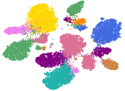
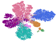
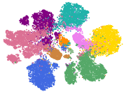
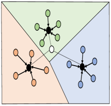
However, in their approach, they represent each class with a single prototype obtained by averaging over the same class space for each client, which can be considered intuitively incomplete and ambiguous [29]. For instance, consider the class of dogs, which includes various breeds differing in size, color, or appearance. Averaging all the dogs within the same class may not adequately capture the diversity and distinctive features present in different dog breeds. This limitation could lead to a less expressive and less discriminative representation for each class, potentially impacting the overall model’s performance in scenarios with intra-class variations. Here, we consider a toy example as shown in Figure 1 to illustrate this intuition. The figure showcases the embeddings in the class space during local training (the upper two subfigures) and federated training (the bottom two subfigures) under the setting of data heterogeneity among clients. It becomes evident from the visualization that there is considerable separation and diversity across the embedding class space in both training scenarios. In local training, each client refines the model using its own data, leading to distinct representations of each class. Similarly, in federated training, where multiple clients collaboratively train the global model, the embedding space still demonstrates significant variations and differentiation. This observation highlights the non-trivial nature of using a single prototype to sufficiently capture the entire embedding space, whether during local or federated training.
Motivated by the above intuition, we introduce MP-FedCL, a strategy that improves the classification performance of FL in scenarios where there is skewness in the distribution of labels and features. The proposed approach uses a contrastive learning scheme, which employs multiple prototypes to represent each class, thereby learning a more differentiated prototype representation in the embedding space for each class. Here, we are inspired by some recent studies [30, 31, 29], which use k-means to cluster features in their methods. For instance, [30] employed k-means clustering to learn a density representation within the embedding space. Moreover, in recent studies by [31, 29], a method for calculating multiple prototypes based on k-means clustering was proposed and achieved good results in image classification tasks. These findings highlight the effectiveness of using k-means clustering to perform feature-based clustering. However, it has not been validated in the FL setting, and our scheme is the first new attempt to introduce the concept of multi-prototype into FL. Specifically, our proposed strategy first applies the k-means clustering algorithm to multiple prototypes calculation, in which each client can calculate their own multiple prototypes for each class. Note that considering the ever-increasing computing capabilities of local clients [5, 32, 33] and privacy issues caused by transferring raw data features [34, 35, 36], we apply the k-means clustering on the feature space on the local side. Due to the natural clustering properties of k-means, the output (i.e. centroids) of k-means clustering algorithm can be viewed as the calculated multiple prototypes for that class. These calculated prototypes from various distributed clients are then sent to the edge server for aggregation as a global prototype pool. The global prototype pool is a combination of multiple prototypes from each client, and it can be updated during training in each global round. To regularize individual local training, we reformulate the local objective of each client in a contrastive learning manner by conducting any supervised learning task (e.g. a cross-entropy loss) and a contrastive learning task. The goal of the contrastive learning task is that prototypes in the global prototype pool and local representations belonging to the same class are pulled together while simultaneously pushing apart those prototypes from different classes. Note that the k-means clustering algorithm is conducted on the local side, and the prototype is a one-dimensional vector of low-dimensional samples that are naturally small and privacy-preserving, which does not incur excessive communication costs or raise privacy concerns compared to the model parameters. To the best of our knowledge, we are the first to present multi-prototype learning in FL. The preliminary version of this work has been published in [16] where we design a multi-prototype-based federated training framework for model inference in the last global iteration based on the typical federated training process. The major differences between the current work and [16] are the addition of the global prototype pool based on a contrastive learning strategy, the modification of the global iteration process, and the exploration of the feature distribution skewness. Our main contributions to this paper are as follows:
-
We introduce a k-means-based multi-prototype federated contrastive learning (MP-FedCL) framework, designed to capture both intra-class and inter-device information. The former can be achieved through the multi-prototype strategy, while the latter can be accomplished by the global prototype pool for information exchange.
-
We reformulate the loss function for each client to perform both supervised learning and contrastive learning tasks. This strategy can encourage each client to learn their own supervised learning task, while also learning from the global prototype pool.
-
We demonstrate that our proposed strategy outperforms several baselines on multiple benchmark datasets regarding test accuracy and communication efficiency, with improvements of about 4.6% and 10.4% under feature and label skewness, respectively.
The remainder of this article is organized as follows. Related work on federated learning and prototype learning is presented in Section II. The system model and problem formulation are provided in Section III. The strategy for multi-prototype computation and aggregation, as well as the model inference, are presented in Section IV. Experimental results are provided in Section V. Finally, conclusions are drawn in Section VI.
II Related Work
In this section, we first review the existing works to deal with FL challenges in Section II-A, including the statistical and system heterogeneity, and communication efficiency. Then, we briefly review some works that apply prototype learning to FL in Section II-B, followed by a schematic diagram of our proposed multi-prototype FL, which will be explained in detail in the next section.
II-A Federated Learning
One of the key challenges in FL is the distribution of training data across multiple clients, which is usually statistically heterogeneous (also known as the non-IID issue). This heterogeneity can limit the effectiveness and performance of FL. Many existing works [37, 38, 39, 40, 41, 42] are dedicated to improving communication efficiency under the challenge of statistical heterogeneity. Other works [43, 44, 45, 46, 47] are mainly from the perspective of system heterogeneity, dealing with communication efficiency issues under the system heterogeneity.
To tackle the system heterogeneity, FedAT [43] introduces an asynchronous layer in which clients are grouped according to their system-specific capabilities to avoid the straggler problem, thus reducing the total number of communication rounds. Unlike typical federated training processes, which are usually implemented with synchronous approaches and can cause stragglers and heterogeneous latency, FedAsync [44] combines asynchronous training with federated training to tackle that issue. To solve the lag or dropout problems of distributed edge devices during federated training, ASO-Fed [45] presents an online federated learning strategy, in which edge devices use continuous streaming local data for online learning and an edge server aggregated model parameters from clients in an asynchronous manner. Sageflow [46] proposes a robust FL framework to cope with both stragglers and adversaries problems. In this framework, clients are grouped and weighted according to their staleness (i.e., arrival delay). Then, entropy-based filtering and loss-weighted averaging are applied within each group to defend against attacks from malicious adversaries. Another asynchronous FL framework in a wireless network environment is proposed in [47]. The framework aims to adapt to environments with heterogeneous edge devices, communication environments, and learning tasks by considering possible delays in local training and uploading local model parameters, as well as the freshness between received models. However, most of these works do not consider the statistical heterogeneity which is the major challenge in FL.
To address the statistical heterogeneity, FedNova [37] suggests that different clients can perform a different number of local steps when updating their shared global model with their local private data. SCAFFOLD[38] introduces two control variables which contain the updated direction information of the global model and local models to overcome the gradient difference and effectively alleviate client drift problems. CMFL [39] designs a feedback mechanism that can reflect the updated trend of the global model. Each client in the system checks whether it is consistent with the update trend of the global model before uploading its model updates to the edge server, otherwise, it does not upload. This strategy of uploading only information related to model improvement to the server greatly reduces communication overhead. FedMMD [40] employs a two-stream model to extract a more generalized representation by minimizing the maximum mean difference (MMD) loss, which is a measure of the distance between two data distributions. This approach can accelerate the convergence rate and reduce communication rounds. AFD [41] proposes a dynamical sub-model parameters selection method, in which clients can update their models using a sub-model rather than the whole global model parameters. This sub-model selection strategy is performed by maintaining an independent activation score map for each client. At each round, the server sends a different sub-model for selected clients, and then clients update their respective score maps according to their own local loss function. A similar approach is also considered in Fed-Dropout [42], which adopts a lossy compression way for server-to-client communication while allowing clients to update their models using sub-models of the global model, further reducing communication overhead. However, most of these works do not consider the scenario where clients in FL are under heterogeneous feature distribution.
II-B Prototype Learning
Prototype learning is first proposed by prototype networks [22] in few-shot learning. Its design idea is to use a single prototype to represent one class, where the single prototype is calculated by averaging the embedding vectors within the same class space. Prototype learning has received significant progress in various tasks such as image classification [48], video processing [49], and natural language processing [50] areas. In image classification tasks [48], a class is represented as a single prototype by computing the mean of the feature vectors of that class. In video processing [49], prototypes are obtained by calculating the average feature over different timestamps. In natural language processing tasks [50], taking the average of word embeddings can yield a prototype representation for a sentence. Further, both few-shot learning and FL are based on the scenario of training with a small amount of data: the clients do not have enough data to train their own models. Recently, there have been various successful works using prototypes for federated optimization in computer vision tasks. In FedProto [19], the authors propose to reduce communication overhead by only exchanging prototypes between clients and the server instead of exchanging gradients or model parameters. However, their work does not validate in a more general heterogeneous environment setting such as Dirichlet distribution [21]. An optimized prototype-based FL is proposed in [51] by using margins of prototypical representations learned from distributed heterogeneous data to calculate the deviations of clients and applying these deviations through an attention mechanism to boost model performance. FedProc [26] introduces that global prototypes in the server can be used as a guideline to correct clients’ training in local updates, and they use a contrastive loss to pull each class to be close to the corresponding global prototypes while pushing away from other global prototypes. FedPCL [27] proposes a strategy based on contrastive learning that uses single prototype exchange instead of gradient communication for efficient communication. MOON [52] is designed based on model-level contrastive learning by comparing the representations between the global model and local models. However, most of them focus on each client’s individual learning process while disregarding the collaborative contributions from other clients. Moreover, most of the above-mentioned works adopt to represent the same class using a single prototype, which may fail to capture discriminative embedding representations by naively taking the mean of the feature space [53, 54].
| Notation | Description |
|---|---|
| Heterogeneous dataset of client | |
| Feature space of client | |
| Corresponding label in the feature space of client | |
| Size of dataset | |
| Shared model parameters of global model | |
| Shared global model | |
| Label space set | |
| Number of label space | |
| Probability of sample being classified as the -th class | |
| Indicator function | |
| Empirical risk of client with one-hot encoded labels | |
| Local loss of client | |
| Set of clients | |
| Number of clients | |
| Global loss across all clients | |
| Learning rate | |
| Loss gradient of client | |
| Supervised learning loss | |
| Regularization term | |
| A local representation of one client | |
| Aggregated global prototype set belonging to -th class | |
| One instance in global prototype set | |
| Aggregated global prototype pool from all clients | |
| Feature extraction layers | |
| Decision-making layers | |
| Embedding space of client belong to class | |
| Output of clustering() | |
| Number of for class of -th client | |
| Number of clusters | |
| Averaged value of global prototype set | |
| Number of instance belonging to | |
| Inner (dot) product | |
| Temperature hyperparameter | |
| Set of labels distinct from | |
| Size of | |
| Size of labels distinct from | |
| Predicted label | |
| -norm of a vector | |
| Number of local epoch | |
| Batch size | |
| Number of global communication rounds | |
| Expectation | |
| -Lipschitz | |
| -smooth | |
| -local dissimilar | |
| Stochastic gradient of each client is bounded by | |
| -Lipschitz continuous |
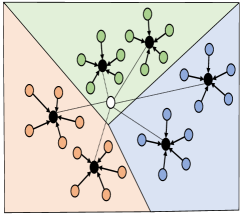
Therefore, different from the single prototype learning paradigm used in these works, we propose to use multiple prototypes to represent each class and adopt multi-prototype-based contrastive learning to capture intra-class differences and inter-class similarities. Here, we briefly describe the core part of the model inference process in the single-prototype-based approach and our proposed multi-prototype-based approach, as shown in Figure 2. Taking the multi-prototype strategy, as illustrated in the right subfigure of Figure 2, as an example, the model inference stage involves two main processes: distance calculation and decision-making. When a query class is introduced to the network during inference, these two processes are executed to determine the most appropriate prototype for the query class. Firstly, the network calculates distances between the new query class and the multiple prototypes associated with each existing class in the class space. These prototypes represent the diverse representations learned from different clients during the FL process. Secondly, the classification decision for the new query class is made based on the shortest distance to any of the prototypes of that specific class. The network assigns the new query class to the class whose prototype exhibits the closest similarity in the embedding space. Note that the multi-prototype concept used in the model inference strategy is also used in our contrastive learning-based model training process. However, the training process differs from the multi-prototype-based model inference process. During the contrastive learning-based model training, the objective is to optimize the query to be as close as possible to multiple prototypes belonging to the same class space while simultaneously ensuring that it remains far away from all other prototypes belonging to class spaces different from its own. The contrastive learning technique aims to enhance the discriminative power of the model by encouraging similar representations for data points belonging to the same class and pushing apart those from different classes. This way, the model learns to create well-separated and informative embeddings for each class, which in turn is expected to benefit the subsequent inference process. The details of the multi-prototype calculation and multi-prototype-based model training and inference will be illustrated in the following sections. Table I presents a summary of the notations used in this manuscript.
III System Model and Problem Formulation
In this section, we first introduce the key elements behind FL, including the system model in Section III-A and the local training optimization algorithm for local training in Section III-B. Then, our optimization problem is formulated in Section III-C.
III-A Federated Learning Model
The essence of the federated learning strategy is to train a model through the collaboration of distributed clients based on their local data, which serves the purpose of protecting data privacy. The overview of the FL framework is shown in Figure 3. The training process can be summarized as follows:
The typical process of federated learning is based on the setting where each client has a heterogeneous and privacy-sensitive dataset, denoted by , of size , where and represent the feature space and corresponding label of the -th client, respectively. The goal is to coordinate the collaboration between clients and the edge server to train a shared model for each client. The empirical risk (e.g., cross-entropy loss) of the client with one-hot encoded labels can be defined as follows [26]:
| (1) |
where is the indicator function, is the shared model parameters of global model, is the number of classes belonging to label space , and denotes the probability of data sample being classified as the -th class. In addition, the local training of each client is to minimize the local loss as follows:
| (2) |
The global objective is to minimize the loss function across heterogeneous clients as follows:
| (3) |
where denotes the set of distributed clients with .
III-B SGD Optimization
As the first FL optimization algorithm, FedAvg requires multiple global iterations during the training process. Most subsequent works [10, 11, 12, 13, 14, 15] follow this training framework, including our work. In each global iteration process, each selected client participates in training and performs local stochastic gradient descent (SGD) to optimize its local objective:
| (4) |
where is the learning rate, is the loss gradient of client , and is the updated result of the global model in the previous round.
III-C Problem Formulation
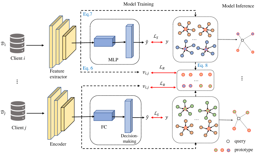
The system model is shown in Figure 4, and the illustration of the transmission of model parameters between clients and the edge server is omitted for simplicity. In each global iteration, the server needs to not only receive model parameters from clients and perform model parameters averaging, but also receive prototype knowledge from clients and aggregate them (the strategy for prototype aggregation will be explained in Section IV-B). Finally, the aggregated model parameters and global prototype pool are returned to local clients participating in the training, while the next iteration begins until convergence. In summary, during the model training phase, clients and with heterogeneous datasets and , respectively, need to simultaneously transmit their own model parameters and their own prototypes based on the features extracted from the feature extraction layers (a.k.a the encoder) to be used in the next global round. Note that the prototypes are the output after clustering, rather than directly averaging the output of the feature extractor layers. The MLP includes the fully connected (FC) layers and a decision-making layer (a.k.a the classifier). In order to extract better features, the former can be an ordinary convolutional layer or a pre-trained network, and the latter is used to map the output of the former from one latent space to another for further representation learning. Each client aims to minimize the typical supervised learning loss , while also minimizing the distance between their local representations and the global prototype pool for samples belonging to the same class space, and maximizing the distance for samples not belonging to the same class space. This can be denoted as . During the model inference stage, the clients can use their individual updated local representations to compare with the updated global prototype pool for model inference. We have marked these entities in the system model and given the basic prototype calculation process.
Specifically, motivated by prototype learning in FL and the observation in their works [53, 54], the goal of this paper is first to learn multi-prototype representations for each class space through the federated training process, and then perform the final model inference based on these prototypes. Formally,
| (5) |
where is a local representation of one client, is defined to aggregate the multiple prototypes for each client belonging to -th class, and denotes one instance in corresponding aggregated global prototype set . Finally, the prediction can be made by measuring the distance between one local representation and each aggregated prototypes set and then choosing the -th label with the smallest distance as the final prediction.
IV Multi-Prototype Federated Learning
In this section, we design an MP-FedCL algorithm to improve the performance of federated training. In Section IV-A, we give the method for calculating multiple prototypes, which is used to compute multiple prototypes in the embedding space for each class based on k-means clustering, thus obtaining a relatively full representation for each class. Then, a strategy for multiple prototypes aggregation is proposed in Section IV-B to collect all class-related knowledge shared by all clients. The objective function of the proposed algorithm is presented in Section IV-C. During the model inference stage, predictions are made based on the distance from the prototypes rather than through a classifier in Section IV-D.
IV-A Multi-Prototype Calculation
The feature extraction layer and the decision-making layer in the MLP are usually two core parts of the deep learning model. The former is mainly used to extract feature information from the input space, and the latter makes the final prediction decision based on the learned feature information. For any client , we denote its feature extraction layers and the MLP as and , then the embedding space of its -th class instance can be calculated as:
| (6) |
where is a set of that belongs to the -th class, and is the embedding space of -th class.
| / | Model Parameters | Multi-Prototype | Ratio |
|---|---|---|---|
| MNIST | 798,474 | 5,120 | 0.006 |
| Digit-5 | 133,898 | 10,240 | 0.076 |
| Office-10 | 133,898 | 10,240 | 0.076 |
| DomainNet | 133,898 | 7,680 | 0.057 |
In order to calculate multiple prototypes for each class, we iteratively cluster into clusters based on k-means algorithm, which is an effective unsupervised algorithm for clustering and has been proven to converge to at least a local optimum after a small number of iterations [55]. Based on the standard iteration of k-means, similarly we also randomly select the centroids in the first iteration. We then calculate the centroid to which each sample in should belong to, and repeat this process until the centroid does not change or changes only slightly. The multiple prototypes used in our method are defined as centroids obtained through k-means clustering. Specifically, we apply k-means clustering to the embeddings of each class, and each resulting centroid is considered a prototype for that class in the embedding space. Thus, multiple prototypes of class can be defined as follows:
| (7) |
where is the number of clusters, the output of Clustering(·) for the -th client of the -th class is denoted as where . Note that because our clustering algorithm is executed on the client side, we need to communicate prototypes with the server, but compared to the complete model parameters, the additional communication cost of prototype communication is very small [56, 19, 57]. The model parameters and the corresponding multi-prototypes, and their ratios are shown in the table II. The Ratio in the Table II is defined as the proportion of multi-prototype to corresponding model parameters, and its result indicates that multi-prototype communication accounts for only a small fraction (less than 0.1) of model parameters. Note that the model architecture and the selection of for multi-prototype are discussed in detail in Section V.
IV-B Multi-Prototype Aggregation
The goal of multi-prototype learning is to reduce the distance of embedding space between local prototypes and the corresponding prototypes from the global prototype pool. After receiving the clustering results as computed in Eq. 7, the server groups these prototypes (also denotes centroids) by class as a global prototype pool. This pool is denoted as = {,,…,}, where each group contains prototypes from the same class but from different clients. Formally,
| (8) |
where denotes the set of clients that own multiple prototypes of class . Through this aggregation mechanism, the prototypes are grouped according to their respective class labels. The resulting global pool summarizes all class-related knowledge shared by all clients, allowing us to effectively utilize information from various clients while maintaining class-wise separation.
After the aggregation process, the server sends back the global prototype pool to local clients, which is used to guide their local training in the next global round. However, some clients’ classes may be missing [26, 58, 59] or underrepresented (i.e., classes with very few samples) [60, 61, 62]. In such cases, the global prototype pool can be utilized to fill in the missing classes and ensure that prototypes for all classes have the same number of prototypes for the learning process. Here, inspired by the single prototype padding approach used in various tasks [63, 27, 64], we introduce a multi-prototype-based padding procedure to achieve a balanced representation of all class prototypes per client. By introducing this prototype padding process, each client is guaranteed to have a consistent and balanced set of prototypes for all classes, regardless of their respective data distribution. Specifically, for the averaging process, the prototypes from different clients are matched based on their respective class labels, which means that prototypes belonging to the same class but originating from different clients are grouped together. Next, we perform the averaging of prototypes by summing up all the prototypes belonging to a particular group and then dividing the sum by the total number of prototypes in that group. Formally,
| (9) |
where represents the averaged value belonging to global prototype set , denotes the number of instance belonging to .
Subsequently, we implement the prototype padding procedure to ensure that each client has a consistent and balanced set of prototypes for every class, which can be formulated as follows:
| (10) |
where is the number of for class of -th client. We traverse all possible prototypes for class of the -th client. For each , we check the number of prototypes currently available for class of the -th client. If is less than , we apply prototype padding by replacing with the averaged prototype . This ensures that each client has prototypes for each class, even in cases where some prototypes might be missing or underrepresented. On the other hand, if equals , it indicates that the client already has the required number of prototypes for class , and no padding is needed. In this case, we keep the -th prototype unchanged.
IV-C Objective Function
As shown in Figure 4, our proposed network architecture consists of two loss functions. The first one, , is the loss of typical supervised learning tasks, which can be computed using Eq. 3. The second one, , is our proposed supervised contrastive loss term. After receiving the global prototype pool from the server, the objective of local clients, , is to align their local representations with the corresponding prototype in the global prototype pool, while simultaneously pushing away dissimilar prototypes from themselves. As such, each client can benefit from other clients. We define the supervised contrastive loss [65] as:
| (11) |
where the symbol denotes the inner (dot) product, is a scalar temperature hyperparameter (the smaller the temperature coefficient, the more focused it is on difficult samples.), represents the local embedding of client , is the set of labels distinct from and the size of is , and denotes one element in a certain global prototype set and the size of one set is .
Therefore, the global objective for the network can be formulated as:
| (12) |
A more detailed model training pseudocode for MP-FedCL is shown in Algorithm 1. The inputs of this algorithm are heterogeneous datasets and some training parameters. After the network is initialized, the federated training process is performed from line 3 to line 20. The multiple prototypes calculation and aggregation are dealt with in lines 19 and 7, respectively. In each global round, the local representations for each client are calculated in line 13. The supervised learning task for them is computed in line 14, and the regularization term is calculated in line 15. After the stochastic gradient descent in the local clients has been performed in line 16, each client then sends their own updated model parameters and calculated multiple prototypes in line 20 back to the server for model parameters aggregation in line 9 and multiple prototypes aggregation in line 7, repeating the above iteration process for rounds until convergence.
Edge server executes:
IV-D Model Inference
Based on the findings of the survey in [66], it is revealed that the lower test accuracy of models in FL environments can be attributed primarily to the later layers of the model. Specifically, the classifier’s predictions have the greatest impact on the model’s accuracy. As a result of this finding, we propose an innovative approach that utilizes the output before the decision-making layer in the model for making predictions instead of relying solely on the classifier. This new approach can be expressed mathematically as a reformulation of Eq. 5:
| (13) |
where is the predicted label, is the output of feature extraction layers (this symbol is originally denoted as in Eq. 5, i.e, the output of feature extraction layers is represented as the local representation), and denotes the -norm of a vector. The prediction can be made by measuring the distance between the local representation and the aggregated prototypes set of -th class. A more detailed model inference pseudocode for MP-FedCL is shown in Algorithm 2. For each client, each sample in its test dataset first calculates the distance to each instance of an aggregated global prototype set in line 4 and then chooses the smallest distance as a candidate-predicted label in line 6. Later, all the candidate-predicted labels are collected in line 8. Finally, the prediction can be made based on the smallest candidate-predicted label in line 9. We also provide a convergence analysis of MP-FedCL in Appendix -A.
IV-E Complexity Analysis
Since Algorithm 1 in MP-FedCL involves many similar global iterations, we analyze the time complexity of only one such iteration for simplicity. In Algorithm 1, each global iteration mainly consists of the following steps: communication round, local model training, and k-means clustering. The algorithm executes a total of global communication rounds. In each round, the global model and the global prototype set are sent to each of the clients in parallel. Therefore, the time complexity for each round can be considered as . For the local model training process, each client performs local updates for a fixed number of local epochs . For the convenience of analysis, let us consider a FC neural network where each layer has the same number of parameters, denoted as . Without loss of generality, we assume that the data samples of each client are the same , given that the batch size is expressed as , the total number of iterations required to complete one local iteration is . In addition, since the computation in each layer can be viewed as a matrix-vector multiplication (note that the matrix calculation mainly involves weight parameters, we ignore bias parameters calculation for simplicity), the time complexity for forward propagation of the FC network in local model training can be expressed as , where represents the number of layers in the FC network. Overall, the time complexity for forward propagation can be simplified as ; here, certain variables , , and can be considered as constants since , , and hold typically. Therefore, the time complexity for local model training is , where the time complexity for back propagation is . After local model training, each client performs k-means clustering to update its embedding space for each class. The time complexity for k-means algorithm is typically , where denotes the number of local epochs, is the number of iterations, is the number of clusters, is the number of data points, is the number of classes, and is the dimensionality of the output before the decision-making layer (here, the output is because it is assumed that parameters of each layer are ). Similarly, certain variables like , , , and can be considered as constants since , , , , then the time complexity for the proposed multi-prototype calculation can be simplified to . Compared with local model training, the time complexity for multi-prototype calculation is relatively low. For Algorithm 2, after the embedding space is calculated, for a certain test sample, the time complexity for model inference is . We assume the number of test samples for each client is , then the total time complexity for model inference is linear as since and can be considered as constants.
V Experiments
We now present the experimental results of the proposed multi-prototype-based federated learning strategy. We implement MP-FedCL on different datasets, and models and compare with the most commonly used baselines including Local, FedAvg [6], FedProx [9], and FedProto [19]. We first introduce the datasets and local models in Section V-A. Then, the implementation details are provided in Section V-B. The selection of for different datasets is discussed in Section V-C. In Section V-D, the test accuracy of different baselines under different datasets with different non-IID settings is illustrated. The robustness and communication efficiency comparison are shown in Section V-E and V-F, respectively.
| Layer | Activation | Value | |
|---|---|---|---|
| Encoder | FC1 | Relu | (28*28, 512) |
| FC2 | Relu | (512, 512) | |
| MLP | FC1 | Relu | (512, 256) |
| FC2 | Relu | (256, 10) |
V-A Datasets and Local Models
We conduct experiments on four popular benchmark datasets: MNIST [67], Digit-5[68], Office-10[69], and DomainNet[70] to verify the potential benefits of multiple-prototype based federated learning for edge network intelligence. MNIST is the handwritten digit recognition dataset. It contains 10 different classes with 60,000 training samples and 10,000 test samples. Digit-5 is a collection of images of handwritten digits from the five most popular datasets, including SVHN, USPS, MNIST, MNIST-M and SynthDigits. Office-10 consists of images from four different office environments, each containing a distinct set of classes: Amazon (A), Webcam (W), DSLR (D), and Caltech (C). DomainNet is a large-scale, multi-domain image classification dataset. It consists of over 600,000 images from 345 categories, divided into 6 domains: clipart, infograph, painting, quickdraw, real, and sketch. Each domain contains a distinct set of classes and has its own characteristics and challenges.
| Parameters | Values |
|---|---|
| Learning rate | 0.01 |
| Learning rate decay | 0.95 |
| Batch size | 32 |
| Local epoch | 1 |
| Temperature | 0.07 |
| Dirichlet parameter | 0.05 (default) |
| Optimizer | SGD |
| SGD momentum | 0.5 |
| (MNIST) | 2 |
| (Digit-5) | 4 |
| (Office-10) | 4 |
| (DomainNet) | 3 |
For local models, a 2-layer encoder network with 2 FC layers and an MLP with 2 FC layers are considered for MNIST, as shown in Table III. For these datasets that are more complex than MNIST, such as Digit-5, Office-10, and DomainNet, we use ResNet18 [71], which has been pre-trained on DomainNet, as the encoder. Please refer to their work [72] for more details about the pre-trained model. We employ the same MLP architecture as in MNIST for these datasets. The output dimension of the encoder and the input of the decision-making layer of the MLP network are 512 and 256, respectively. Note that for fair comparisons, all baselines adopt the same network architecture as MP-FedCL, including MLP.
V-B Implementation Details
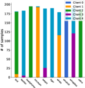
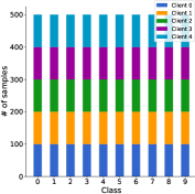
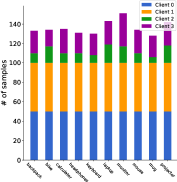
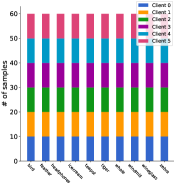
We investigate two different non-IID settings to mimic non-IID scenarios : (i) feature distribution skew: clients have the same label distributions but different feature distributions, (ii) label distribution skew: clients have different label distributions but the same feature distribution, which is simulated by Dirichlet distribution Dir() [21]. Here, the more skewness among clients is, the smaller the value is, and vice versa. The label distribution skewness is set to 0.05 for all federated training algorithms unless explicitly specified.
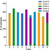
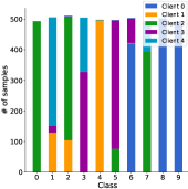
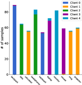
We compare our proposed method with popular FL algorithms including Local where local models are updated in each global round without any communication with others, FedAvg [6], FedProto [19], and FedProx [9]. We use 5, 4, and 6 clients for Digit-5, Office-10, and DomainNet in the feature distribution skewed setting, respectively. In the label distribution skewed setting, the number of clients for Digit-5, Office-10, and DomainNet is all 5. We use 5 clients for MNIST unless explicitly specified. The size of MNIST for all experiments is 2,000 for simplicity. The visualization results of all datasets with label non-IID and feature non-IID settings are shown in Figure 6 and Figure 7, respectively.
We use PyTorch [73] to implement all the baselines. Following [9, 27], the grid search is used to select the optimal hyperparameters for model training. Specifically, we use the SGD optimizer for all baselines, and the SGD momentum is set to 0.5. The other training parameters are set to be = 32, = 1, = 0.07, = 0.01 with decay rate = 0.95, which denotes local batch size, local epochs, temperature, learning rate, and learning rate decay per iteration, respectively.
V-C Choosing
The selection of is performed in the feature space of samples in different datasets. Intuitively, the feature space of samples from different datasets is different; thus the number of is associated with specific datasets. Here, we adopt a similar way as [30] to maintain a uniform value for across classes for simplicity, although this value may vary for different classes. Note that since we focus on the fixed-prototype strategy in this paper, we initially explore a dynamic prototype-based scheme for completeness. Specifically, we study the effect of different under label distribution skew through heuristic selection and then apply the most appropriate value to all experiments under different non-IID settings. Similar heuristic selection method applied in the feature space has been utilized in many papers [74, 31, 16]. We run three trials with different random seeds and report the average test accuracy on validation datasets, as shown in Figure 5. The number of communication rounds is set to 60 for all datasets. It can be found that the appropriate values for MNIST, Digit-5, Office-10, and DomainNet are 2, 4, 4, and 3, respectively. The hyperparameters used are presented in Table IV.
| Method | Local | FedAvg | FedProx | FedProto | MP-FedCL |
| MNIST | 47.33(8.96) | 53.00(4.32) | 72.00(5.89) | 88.00(2.83) | 91.37(0.39) |
| SVHN | 16.67(2.05) | 18.67(1.25) | 22.33(3.30) | 25.00(1.41) | 26.80(2.65) |
| USPS | 60.33(1.25) | 54.67(4.99) | 71.67(5.73) | 91.67(1.25) | 93.93(0.65) |
| Synth | 26.33(6.13) | 36.00(2.94) | 49.33(4.71) | 56.67(1.25) | 61.00(0.49) |
| MNIST-M | 20.33(3.30) | 32.00(4.55) | 43.67(4.11) | 48.67(3.68) | 51.20(1.77) |
| Average | 34.20(4.34) | 38.87(3.61) | 51.80(4.75) | 62.00(2.08) | 64.86(1.19) |
| Method | MNIST | Digit-5 | Office-10 | DomainNet |
|
||
| FedAvg | 66.40(2.89) | 29.66(1.57) | 24.00(1.55) | 23.61(4.35) | 110 | ||
| FedProx | 64.85(1.88) | 28.51(2.13) | 21.74(1.13) | 22.78(5.66) | 100 | ||
| FedProto | 33.27(1.74) | 60.84(1.79) | 39.79(3.15) | 36.02(5.23) | 100 | ||
| DP-FedCL | 78.49(3.09) | 53.94(3.38) | 37.22(1.75) | 47.62(1.78) | 60 | ||
| SP-FedCL | 79.44(3.48) | 57.91(3.17) | 43.11(4.30) | 35.44(4.25) | 60 | ||
| MP-FedCL | 79.95(3.76) | 67.15(2.33) | 59.07(3.41) | 52.12(5.02) | 60 |
V-D Accuracy Comparison
In this section, given that the number of may vary across different classes, we attempt to explore another feature clustering method for feature clustering, called density-based spatial clustering of applications with noise (DBSCAN) [75], which is different from k-means as it does not require specifying the number of clusters beforehand. It automatically determines the number of clusters based on the data’s density and has been applied in the image field [76, 77, 78, 79, 80]. Here, we combine the DBSCAN clustering method with our proposal that each client uses DBSCAN for clustering instead of k-means, terming it DP-FedCL, and compare it with MP-FedCL and other baselines.
Specifically, we compare our method with the baselines under the feature non-IID and label non-IID settings where feature non-IID means the feature distribution is skewed while the label distribution is IID, and label non-IID means the label distribution is skewed while the feature distribution is IID. For the sake of fair comparison, we conduct experiments with the same hyperparameters, run three trials, and report the mean and standard derivation. The best results are shown in bold.
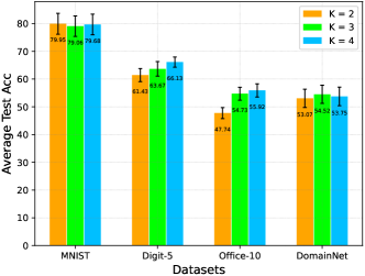
Table V reports the average test accuracies of our method and baselines in the mean(std) format under the feature non-IID setting. The results indicate that MP-FedCL achieves higher test accuracy and smaller standard deviation compared to most cases, with an improvement of approximately 4.6% over the second-highest test accuracy. In addition, Table VI presents our results and those of the baselines under the label non-IID setting. In this setting, we use SP-FedCL, which refers to our training strategy that employs a single prototype (i.e., = 1). Specifically, we do not use any clustering algorithm in Eq. 7, but instead take the mean value of the feature space belonging to the same label as the prototype of the label, which is also known as a single prototype. The results show that our method enjoys relatively significant advantages over almost all other baselines, and about at least 10.4% improvement in test accuracy compared to most cases. Moreover, since the cost of communication has been considered to be the bottleneck of FL, we also report the number of communication rounds for each algorithm in Table VI accordingly. It can be seen that our proposal and other methods based on our strategy only need relatively few communication rounds compared to others. For DP-FedCL, the only difference from MP-FedCL is that it dynamically selects the number of clusters using the DBSCAN algorithm on each local client. The results indicate that clustering using k-means and assigning an equal number of prototypes to each class outperforms the adopted dynamic selection approach. We conjecture that while dynamically selecting the number of clusters might lead to varying prototype assignments for each class, it can also introduce an imbalance in class representations, resulting in biased model learning.
V-E Robustness Comparison
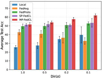
Different degrees of label non-IID. Considering that labeling non-IID is a common challenge in FL, designing an algorithm that is robust to various heterogeneous data is crucial for deploying the FL algorithm in real applications. Therefore, we compare our method with several baselines under different levels of label heterogeneity to verify the robustness of different algorithms to data heterogeneity. As shown in Figure 8, the decreases from 1.0 to 0.1, controlling the degree of label heterogeneity, which means that labels are distributed more and more heterogeneously among clients. We report the average test accuracy for Digit-5 under different heterogeneities in Figure 8 (a). Note that since our proposal requires only a small number of iterations, therefore the number of communication rounds for MP-FedCL and SP-FedCL is set to 60, and 100 for others. The results show that our proposal outperforms all approaches under different heterogeneous settings in terms of test accuracy, and enjoys a relatively small deviation compared to those in most cases.
Specifically, in comparison to the performance under all heterogeneity settings, our method achieves at least an 8.8% and 2.0% increase in accuracy compared to the popular baseline FedAvg and state-of-the-art FedProto, respectively. To highlight the advantage of multi-prototype learning over single-prototype learning, we conduct experiments using the same learning strategy as the former, but with only a single prototype, which we refer to as SP-FedCL. The results show that our method consistently outperforms SP-FedCL by approximately 2.0% in average test accuracy across various scenarios. These results underscore the effectiveness of our multi-prototype learning approach in FL, leading to improved robustness compared to both single-prototype and state-of-the-art methods. Interestingly, in some scenarios (such as ), the performance of FedAvg is lower than that of Local, which shows that FedAvg does not always perform well in dealing with heterogeneous scenarios. It would be an intriguing research direction to explore the synergies between local optimization and federated optimization, allowing us to harness the advantages offered by both approaches.
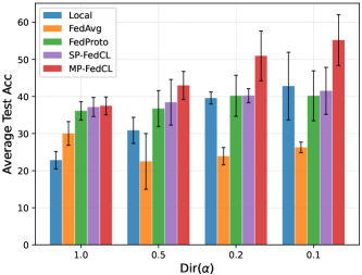
Additionally, in Figure 8 (b), we present similar results for Office-10 under various degrees of heterogeneity. The findings further demonstrate that, in the majority of cases, our proposed method outperforms all other approaches in terms of test accuracy, highlighting its advantage in dealing with data heterogeneity. Specifically, compared to SP-FedCL, FedProto, and FedAvg, our method shows improvements of at least 0.3%, 1.4%, and 7.5%, respectively, across different label non-IID settings. However, it is worth noting that almost all methods, including ours, encounter significant deviations under extremely heterogeneous settings like Dir(0.1) and Dir(0.2). This can be attributed to the relatively limited number of training samples available in Office-10 compared to Digit-5, which may lead to higher fluctuations in performance. Moreover, it should be noted that similar results are observed in this setting, with FedAvg performing worse than Local in most cases.
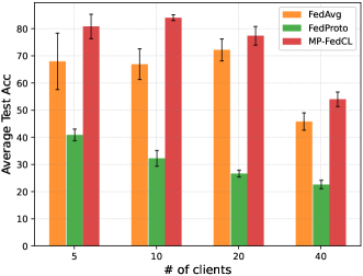
Different numbers of clients. In addition to exploring the robustness of our proposed algorithm to different levels of data heterogeneity, we also aim to investigate its robustness to varying numbers of participating clients in the FL setting. As depicted in Figure 9, we demonstrate the robustness of our proposed method by evaluating its performance across an increasing number of clients, ranging from 5 to 40, with labels distribution following Dir(0.1). The average test accuracy for MNIST and Digit-5 under the various number of clients is shown in Figure 9 (a) and Figure 9 (b), respectively. The illustration demonstrates that our proposed method exhibits a distinct advantage over FedAvg in terms of test accuracy across different numbers of clients. Moreover, our approach maintains a relatively small deviation compared to FedAvg in most cases, further highlighting its robustness against various numbers of clients.
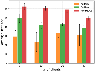
Specifically, regarding the results of MNIST displayed in Figure 9 (a), our proposed method achieves a remarkable increase of at least 7.2% in test accuracy compared to the baseline FedAvg when varying the number of clients. It is interesting to note that, compared to both FedAvg and MP-FedCL, FedProto exhibits inferior performance across all numbers of participating clients. Moreover, the performance of FedProto decreases as the number of clients increases, and its peak performance is only about half of that of MP-FedCL. This observation strongly suggests that the approach of not transmitting the model parameters, as adopted in FedProto, may not be suitable for models trained from scratch. Similarly, in the case of Digit-5, as shown in Figure 9 (b), our proposal consistently outperforms both FedAvg and FedProto in terms of test accuracy across different numbers of clients. To be precise, our method demonstrates an improvement of at least 18.73% and 10.99% compared to FedAvg and FedProto, respectively. Furthermore, it is worthwhile to mention that our proposed method exhibits lower accuracy variance compared to the other methods in the majority of cases, whereas FedAvg experiences higher fluctuations. This observation could be attributed to the inherent complexity of the feature space in Digit-5, which is likely more intricate compared to the MNIST dataset. Consequently, the variations between clients in Digit-5 become more pronounced, leading to the observed differences in performance for FedAvg. In contrast, prototype-based schemes such as FedProto and MP-FedCL show more robust results (in terms of accuracy variation) across different numbers of participating clients in the FL setting. This indicates that an approach based on prototypes successfully handles heterogeneity to a certain extent.
| Dataset | Method | Label non-IID | Feature non-IID |
|
||
|---|---|---|---|---|---|---|
| Local | 27.60(3.33) | 33.60(3.25) | 0 | |||
| FedAvg | 40.80(3.71) | 43.13(3.67) | 130 | |||
| Digit-5 | FedProto | 49.71(2.98) | 63.99(0.38) | 130 | ||
| DP-FedCL | 50.37(2.51) | 63.49(2.02) | 60 | |||
| SP-FedCL | 51.86(2.92) | 65.49(1.14) | 60 | |||
| MP-FedCL | 53.87(1.62) | 65.08(0.91) | 60 | |||
| Local | 30.89(3.50) | 21.47(3.72) | 0 | |||
| FedAvg | 22.51(7.50) | 30.17(2.15) | 130 | |||
| Office-10 | FedProto | 36.75(3.50) | 46.58(2.82) | 130 | ||
| DP-FedCL | 35.74(5.33) | 42.77(1.03) | 60 | |||
| SP-FedCL | 38.44(6.15) | 48.88(3.59) | 60 | |||
| MP-FedCL | 42.98(3.79) | 49.70(1.49) | 60 |
V-F Communication Efficiency Comparison
As FL involves training models across distributed clients, ensuring a fast and efficient convergence rate is of great importance. A faster convergence rate implies that the participating clients can converge to the optimal with higher accuracy in fewer communication rounds, reducing the overall communication and computational overhead. Therefore, in this section, we evaluate the convergence rate of our proposal and conduct a comprehensive investigation with other benchmarks.
Table VII presents the top-1 average test accuracy (%) of different methods, including Local, FedAvg, FedProto, DP-FedCL, SP-FedCL, and MP-FedCL, on two datasets: Digit-5 and Office-10 and the corresponding communication rounds. The evaluation is performed under the condition of label non-IID with Dir(0.5) and feature non-IID. From the results in Table VII, we observe that MP-FedCL consistently achieves the highest top-1 average test accuracy and fewer communication rounds compared to other methods in most cases. Specifically, Local achieves the lowest accuracy since it does not participate in FL rounds (0 communication rounds). The methods based on federated training such as FedAvg and FedProto, have shown improved performance, but they require a high number of communication rounds (130 communication rounds). In contrast, MP-FedCL consistently outperforms the other federated methods in most cases and only requires about half the number of communication rounds (60 communication rounds) of FedAvg, showcasing its capability to learn from distributed data efficiently. In other words, achieving similar performance to the baselines MP-FedCL requires fewer computational resources. Moreover, we observe a similar phenomenon as in Table VI that DP-FedCL is still lower than the single-prototype scheme and our proposal in this setting. However, it is worthwhile to note that other schemes for dynamically selecting prototypes may potentially outperform our current approach, which leaves for our future work.
| Dataset | Method | Label non-IID |
|
Feature non-IID |
|
||||
|---|---|---|---|---|---|---|---|---|---|
| FedAvg | 38.17(1.26) | 600 | 43.00(3.49) | 600 | |||||
| FedProto | 52.67(1.03) | 600 | 62.00(2.69) | 600 | |||||
| Digit-5 | DP-FedCL | 52.42(1.83) | 600 | 64.07(2.07) | 600 | ||||
| SP-FedCL | 52.46(1.58) | 600 | 65.07(1.89) | 600 | |||||
| MP-FedCL | 52.94(1.68) | 600 | 65.00(1.47) | 600 | |||||
| FedAvg | 23.59(5.69) | 380 | 24.04(2.61) | 380 | |||||
| FedProto | 39.11(6.99) | 380 | 45.34(2.72) | 380 | |||||
| Office-10 | DP-FedCL | 35.98(5.95) | 380 | 41.83(2.14) | 380 | ||||
| SP-FedCL | 39.60(5.89) | 380 | 45.20(3.56) | 380 | |||||
| MP-FedCL | 43.59(5.54) | 380 | 47.38(1.48) | 380 |
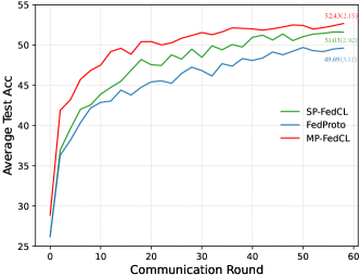
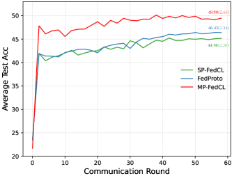
Table VIII shows the top-1 average test accuracy of MP-FedCL and other baselines on Digit-5 and Office-10 under label non-IID with Dir(0.5) and feature non-IID. All algorithms are compared under similar training times. The results show that MP-FedCL achieves comparable or superior performance compared to baselines. In other words, MP-FedCL can still achieve competitive performance under approximately the same computational resources. In addition, we compare the average test accuracy of our proposed MP-FedCL with FedProto and SP-FedCL per global round during training based on different kinds of heterogeneous settings (including feature non-IID and label non-IID) after several runs with different random seeds, as shown in Figure 10. Both subfigures demonstrate that our method outperforms them in terms of test accuracy and communication efficiency. Specifically, we evaluate our proposal with FedProto and SP-FedCL on Digit-5 under label non-IID with Dir(1.0). It shows that our method outperforms theirs by approximately 2.74% and 1.40% in test accuracy, respectively, and also leads them the way in convergence rate. Similar results are available in Figure 10 (b), which is the test accuracy of Office-10 with feature non-IID. It demonstrates that our proposal still outperforms theirs by 3.47% and 4.92% in terms of test accuracy, and they lag behind us by a significant margin in terms of convergence rate. This indicates the potential advantages of using multi-prototype learning in handling heterogeneous tasks in FL, and we believe that multi-prototype learning based on architectures such as transformers will be a promising research direction in the future. Moreover, it can be expected that combining strategies aimed at accelerating k-means calculation and other privacy-preserving techniques with our strategy will further make contributions to the FL community.
VI Conclusion
In this paper, we have introduced multi-prototype learning into the federated learning framework, and at the same time, a contrastive learning strategy is applied to multi-prototype learning to make full use of multi-prototype knowledge. First, a clustering-based multi-prototype calculation approach has been proposed. In order to better leverage the knowledge from each client, we then have proposed a contrastive learning strategy that encourages clients to learn class-related knowledge from others in each global round through multi-prototype exchange, while reducing the absorption of class-unrelated knowledge. Further, we have introduced a multi-prototype-based model inference strategy into FL. This strategy also provides the potential for fast model training in distributed edge networks, as only a small amount of training is required when adding a new client, to compare its prototype with the trained prototypes in the global prototype pool for fast and correct predictions. Finally, extensive experiments on four datasets demonstrate that our proposal has a robust performance against label and feature heterogeneity in terms of test accuracy and communication efficiency. Compared to several baselines, our test accuracy improves by about 4.6% and 10.4% under feature and label non-IID, respectively.
References
- [1] M. Asif-Ur-Rahman, F. Afsana, M. Mahmud, M. S. Kaiser, M. R. Ahmed, O. Kaiwartya, and A. James-Taylor, “Toward a heterogeneous mist, fog, and cloud-based framework for the internet of healthcare things,” IEEE Internet of Things Journal, vol. 6, no. 3, pp. 4049–4062, 2018.
- [2] W. Shi, J. Cao, Q. Zhang, Y. Li, and L. Xu, “Edge computing: Vision and challenges,” IEEE internet of things journal, vol. 3, no. 5, pp. 637–646, 2016.
- [3] S. Deng, H. Zhao, W. Fang, J. Yin, S. Dustdar, and A. Y. Zomaya, “Edge intelligence: The confluence of edge computing and artificial intelligence,” IEEE Internet of Things Journal, vol. 7, no. 8, pp. 7457–7469, 2020.
- [4] M. Magdziarczyk, “Right to be forgotten in light of regulation (eu) 2016/679 of the european parliament and of the council of 27 april 2016 on the protection of natural persons with regard to the processing of personal data and on the free movement of such data, and repealing directive 95/46/ec,” in 6th International Multidisciplinary Scientific Conference on Social Sciences and Art Sgem 2019, 2019, pp. 177–184.
- [5] H. Wu and P. Wang, “Node selection toward faster convergence for federated learning on non-iid data,” IEEE Transactions on Network Science and Engineering, vol. 9, no. 5, pp. 3099–3111, 2022.
- [6] B. McMahan, E. Moore, D. Ramage, S. Hampson, and B. A. y Arcas, “Communication-efficient learning of deep networks from decentralized data,” in Artificial intelligence and statistics. PMLR, 2017, pp. 1273–1282.
- [7] J. Park, S. Samarakoon, M. Bennis, and M. Debbah, “Wireless network intelligence at the edge,” Proceedings of the IEEE, vol. 107, no. 11, pp. 2204–2239, 2019.
- [8] P. Kairouz, H. B. McMahan, B. Avent, A. Bellet, M. Bennis, A. N. Bhagoji, K. Bonawitz, Z. Charles, G. Cormode, R. Cummings et al., “Advances and open problems in federated learning,” Foundations and Trends® in Machine Learning, vol. 14, no. 1–2, pp. 1–210, 2021.
- [9] T. Li, A. K. Sahu, M. Zaheer, M. Sanjabi, A. Talwalkar, and V. Smith, “Federated optimization in heterogeneous networks,” Proceedings of Machine learning and systems, vol. 2, pp. 429–450, 2020.
- [10] J. Zhang, Z. Li, B. Li, J. Xu, S. Wu, S. Ding, and C. Wu, “Federated learning with label distribution skew via logits calibration,” in International Conference on Machine Learning. PMLR, 2022, pp. 26 311–26 329.
- [11] G. Long, M. Xie, T. Shen, T. Zhou, X. Wang, and J. Jiang, “Multi-center federated learning: clients clustering for better personalization,” World Wide Web, vol. 26, no. 1, pp. 481–500, 2023.
- [12] Y. Qiao, M. S. Munir, A. Adhikary, A. D. Raha, and C. S. Hong, “Cdfed: Contribution-based dynamic federated learning for managing system and statistical heterogeneity,” in NOMS 2023-2023 IEEE/IFIP Network Operations and Management Symposium. IEEE, 2023, pp. 1–5.
- [13] C. T Dinh, N. Tran, and J. Nguyen, “Personalized federated learning with moreau envelopes,” Advances in Neural Information Processing Systems, vol. 33, pp. 21 394–21 405, 2020.
- [14] A. Fallah, A. Mokhtari, and A. Ozdaglar, “Personalized federated learning: A meta-learning approach,” arXiv preprint arXiv:2002.07948, 2020.
- [15] M. G. Arivazhagan, V. Aggarwal, A. K. Singh, and S. Choudhary, “Federated learning with personalization layers,” arXiv preprint arXiv:1912.00818, 2019.
- [16] Y. Qiao, M. S. Munir, A. Adhikary, A. D. Raha, S. H. Hong, and C. S. Hong, “A framework for multi-prototype based federated learning: Towards the edge intelligence,” in 2023 International Conference on Information Networking (ICOIN). IEEE, 2023, pp. 134–139.
- [17] H. Zhu, J. Xu, S. Liu, and Y. Jin, “Federated learning on non-iid data: A survey,” Neurocomputing, vol. 465, pp. 371–390, 2021.
- [18] Q. Li, Y. Diao, Q. Chen, and B. He, “Federated learning on non-iid data silos: An experimental study,” in 2022 IEEE 38th International Conference on Data Engineering (ICDE). IEEE, 2022, pp. 965–978.
- [19] Y. Tan, G. Long, L. Liu, T. Zhou, Q. Lu, J. Jiang, and C. Zhang, “Fedproto: Federated prototype learning across heterogeneous clients,” in Proceedings of the AAAI Conference on Artificial Intelligence, vol. 36, no. 8, 2022, pp. 8432–8440.
- [20] L. Van der Maaten and G. Hinton, “Visualizing data using t-sne.” Journal of machine learning research, vol. 9, no. 11, 2008.
- [21] M. Yurochkin, M. Agarwal, S. Ghosh, K. Greenewald, N. Hoang, and Y. Khazaeni, “Bayesian nonparametric federated learning of neural networks,” in International conference on machine learning. PMLR, 2019, pp. 7252–7261.
- [22] J. Snell, K. Swersky, and R. Zemel, “Prototypical networks for few-shot learning,” Advances in neural information processing systems, vol. 30, 2017.
- [23] R. Hou, Z. Chen, J. Chen, S. He, and Z. Zhou, “Imbalanced fault identification via embedding-augmented gaussian prototype network with meta-learning perspective,” Measurement Science and Technology, vol. 33, no. 5, p. 055102, 2022.
- [24] Z. Kang, K. Grauman, and F. Sha, “Learning with whom to share in multi-task feature learning,” in Proceedings of the 28th International Conference on Machine Learning (ICML-11), 2011, pp. 521–528.
- [25] A. Quattoni, M. Collins, and T. Darrell, “Transfer learning for image classification with sparse prototype representations,” in 2008 IEEE Conference on Computer Vision and Pattern Recognition. IEEE, 2008, pp. 1–8.
- [26] X. Mu, Y. Shen, K. Cheng, X. Geng, J. Fu, T. Zhang, and Z. Zhang, “Fedproc: Prototypical contrastive federated learning on non-iid data,” Future Generation Computer Systems, vol. 143, pp. 93–104, 2023.
- [27] Y. Tan, G. Long, J. Ma, L. Liu, T. Zhou, and J. Jiang, “Federated learning from pre-trained models: A contrastive learning approach,” Advances in Neural Information Processing Systems, vol. 35, pp. 19 332–19 344, 2022.
- [28] Y. Qiao, S.-B. Park, S. M. Kang, and C. S. Hong, “Prototype helps federated learning: Towards faster convergence,” arXiv preprint arXiv:2303.12296, 2023.
- [29] H. Huang, Z. Wu, W. Li, J. Huo, and Y. Gao, “Local descriptor-based multi-prototype network for few-shot learning,” Pattern Recognition, vol. 116, p. 107935, 2021.
- [30] O. Rippel, M. Paluri, P. Dollar, and L. Bourdev, “Metric learning with adaptive density discrimination,” arXiv preprint arXiv:1511.05939, 2015.
- [31] J. Deuschel, D. Firmbach, C. I. Geppert, M. Eckstein, A. Hartmann, V. Bruns, P. Kuritcyn, J. Dexl, D. Hartmann, D. Perrin et al., “Multi-prototype few-shot learning in histopathology,” in Proceedings of the IEEE/CVF international conference on computer vision, 2021, pp. 620–628.
- [32] Y.-J. Liu, S. Qin, G. Feng, D. Niyato, Y. Sun, and J. Zhou, “Adaptive quantization based on ensemble distillation to support fl enabled edge intelligence,” in GLOBECOM 2022-2022 IEEE Global Communications Conference. IEEE, 2022, pp. 2194–2199.
- [33] M. Beitollahi and N. Lu, “Federated learning over wireless networks: Challenges and solutions,” IEEE Internet of Things Journal, 2023.
- [34] Y. Zhang, Y. Hu, X. Gao, D. Gong, Y. Guo, K. Gao, and W. Zhang, “An embedded vertical-federated feature selection algorithm based on particle swarm optimisation,” CAAI Transactions on Intelligence Technology, 2022.
- [35] M. Alazab, S. P. RM, M. Parimala, P. K. R. Maddikunta, T. R. Gadekallu, and Q.-V. Pham, “Federated learning for cybersecurity: Concepts, challenges, and future directions,” IEEE Transactions on Industrial Informatics, vol. 18, no. 5, pp. 3501–3509, 2021.
- [36] A. Anaissi, B. Suleiman, and M. Naji, “Intelligent structural damage detection: a federated learning approach,” in Advances in Intelligent Data Analysis XIX: 19th International Symposium on Intelligent Data Analysis, IDA 2021, Porto, Portugal, April 26–28, 2021, Proceedings 19. Springer, 2021, pp. 155–170.
- [37] J. Wang, Q. Liu, H. Liang, G. Joshi, and H. V. Poor, “Tackling the objective inconsistency problem in heterogeneous federated optimization,” Advances in neural information processing systems, vol. 33, pp. 7611–7623, 2020.
- [38] S. P. Karimireddy, S. Kale, M. Mohri, S. Reddi, S. Stich, and A. T. Suresh, “Scaffold: Stochastic controlled averaging for federated learning,” in International Conference on Machine Learning. PMLR, 2020, pp. 5132–5143.
- [39] W. Luping, W. Wei, and L. Bo, “Cmfl: Mitigating communication overhead for federated learning,” in 2019 IEEE 39th international conference on distributed computing systems (ICDCS). IEEE, 2019, pp. 954–964.
- [40] X. Yao, T. Huang, C. Wu, R.-X. Zhang, and L. Sun, “Federated learning with additional mechanisms on clients to reduce communication costs,” arXiv preprint arXiv:1908.05891, 2019.
- [41] N. Bouacida, J. Hou, H. Zang, and X. Liu, “Adaptive federated dropout: Improving communication efficiency and generalization for federated learning,” arXiv preprint arXiv:2011.04050, 2020.
- [42] S. Caldas, J. Konečny, H. B. McMahan, and A. Talwalkar, “Expanding the reach of federated learning by reducing client resource requirements,” arXiv preprint arXiv:1812.07210, 2018.
- [43] Z. Chai, Y. Chen, A. Anwar, L. Zhao, Y. Cheng, and H. Rangwala, “Fedat: a high-performance and communication-efficient federated learning system with asynchronous tiers,” in Proceedings of the International Conference for High Performance Computing, Networking, Storage and Analysis, 2021, pp. 1–16.
- [44] C. Xie, S. Koyejo, and I. Gupta, “Asynchronous federated optimization,” arXiv preprint arXiv:1903.03934, 2019.
- [45] Y. Chen, Y. Ning, M. Slawski, and H. Rangwala, “Asynchronous online federated learning for edge devices with non-iid data,” in 2020 IEEE International Conference on Big Data (Big Data). IEEE, 2020, pp. 15–24.
- [46] J. Park, D.-J. Han, M. Choi, and J. Moon, “Handling both stragglers and adversaries for robust federated learning,” in ICML 2021 Workshop on Federated Learning for User Privacy and Data Confidentiality. ICML Board, 2021.
- [47] Z. Wang, Z. Zhang, Y. Tian, Q. Yang, H. Shan, W. Wang, and T. Q. Quek, “Asynchronous federated learning over wireless communication networks,” IEEE Transactions on Wireless Communications, vol. 21, no. 9, pp. 6961–6978, 2022.
- [48] U. Michieli and P. Zanuttigh, “Continual semantic segmentation via repulsion-attraction of sparse and disentangled latent representations,” in Proceedings of the IEEE/CVF conference on computer vision and pattern recognition, 2021, pp. 1114–1124.
- [49] G. Xue, M. Zhong, J. Li, J. Chen, C. Zhai, and R. Kong, “Dynamic network embedding survey,” Neurocomputing, vol. 472, pp. 212–223, 2022.
- [50] J. Wieting, M. Bansal, K. Gimpel, and K. Livescu, “Towards universal paraphrastic sentence embeddings,” arXiv preprint arXiv:1511.08198, 2015.
- [51] U. Michieli and M. Ozay, “Prototype guided federated learning of visual feature representations,” arXiv preprint arXiv:2105.08982, 2021.
- [52] Q. Li, B. He, and D. Song, “Model-contrastive federated learning,” in Proceedings of the IEEE/CVF conference on computer vision and pattern recognition, 2021, pp. 10 713–10 722.
- [53] X. Li, T. Tian, Y. Liu, H. Yu, J. Cao, and Z. Ma, “Adaptive multi-prototype relation network,” in 2020 Asia-Pacific Signal and Information Processing Association Annual Summit and Conference (APSIPA ASC). IEEE, 2020, pp. 1707–1712.
- [54] G. Li, V. Jampani, L. Sevilla-Lara, D. Sun, J. Kim, and J. Kim, “Adaptive prototype learning and allocation for few-shot segmentation,” in Proceedings of the IEEE/CVF conference on computer vision and pattern recognition, 2021, pp. 8334–8343.
- [55] A. Géron, Hands-on machine learning with Scikit-Learn, Keras, and TensorFlow. ” O’Reilly Media, Inc.”, 2022.
- [56] C. He, M. Annavaram, and S. Avestimehr, “Group knowledge transfer: Federated learning of large cnns at the edge,” Advances in Neural Information Processing Systems, vol. 33, pp. 14 068–14 080, 2020.
- [57] W. Lou, Y. Xu, H. Xu, and Y. Liao, “Decentralized federated learning with data feature transmission and neighbor selection,” in 2022 IEEE 28th International Conference on Parallel and Distributed Systems (ICPADS). IEEE, 2023, pp. 688–695.
- [58] X.-C. Li and D.-C. Zhan, “Fedrs: Federated learning with restricted softmax for label distribution non-iid data,” in Proceedings of the 27th ACM SIGKDD Conference on Knowledge Discovery & Data Mining, 2021, pp. 995–1005.
- [59] Z. Zhou, S. S. Azam, C. Brinton, and D. I. Inouye, “Efficient federated domain translation,” in The Eleventh International Conference on Learning Representations, 2022.
- [60] M. Servetnyk, C. C. Fung, and Z. Han, “Unsupervised federated learning for unbalanced data,” in GLOBECOM 2020-2020 IEEE Global Communications Conference. IEEE, 2020, pp. 1–6.
- [61] Y. Fraboni, R. Vidal, L. Kameni, and M. Lorenzi, “Clustered sampling: Low-variance and improved representativity for clients selection in federated learning,” in International Conference on Machine Learning. PMLR, 2021, pp. 3407–3416.
- [62] X. Shuai, Y. Shen, S. Jiang, Z. Zhao, Z. Yan, and G. Xing, “Balancefl: Addressing class imbalance in long-tail federated learning,” in 2022 21st ACM/IEEE International Conference on Information Processing in Sensor Networks (IPSN). IEEE, 2022, pp. 271–284.
- [63] D. Pal, S. Bose, B. Banerjee, and Y. Jeppu, “Extreme value meta-learning for few-shot open-set recognition of hyperspectral images,” IEEE Transactions on Geoscience and Remote Sensing, 2023.
- [64] J. Zhou, J. Mei, H. Li, and Y. Hu, “Pmr-cnn: Prototype mixture r-cnn for few-shot object detection,” in 2023 IEEE Intelligent Vehicles Symposium (IV). IEEE, 2023, pp. 1–7.
- [65] P. Khosla, P. Teterwak, C. Wang, A. Sarna, Y. Tian, P. Isola, A. Maschinot, C. Liu, and D. Krishnan, “Supervised contrastive learning,” Advances in neural information processing systems, vol. 33, pp. 18 661–18 673, 2020.
- [66] M. Luo, F. Chen, D. Hu, Y. Zhang, J. Liang, and J. Feng, “No fear of heterogeneity: Classifier calibration for federated learning with non-iid data,” Advances in Neural Information Processing Systems, vol. 34, pp. 5972–5984, 2021.
- [67] Y. LeCun, L. Bottou, Y. Bengio, and P. Haffner, “Gradient-based learning applied to document recognition,” Proceedings of the IEEE, vol. 86, no. 11, pp. 2278–2324, 1998.
- [68] K. Zhou, Y. Yang, T. Hospedales, and T. Xiang, “Learning to generate novel domains for domain generalization,” in Computer Vision–ECCV 2020: 16th European Conference, Glasgow, UK, August 23–28, 2020, Proceedings, Part XVI 16. Springer, 2020, pp. 561–578.
- [69] B. Gong, Y. Shi, F. Sha, and K. Grauman, “Geodesic flow kernel for unsupervised domain adaptation,” in 2012 IEEE conference on computer vision and pattern recognition. IEEE, 2012, pp. 2066–2073.
- [70] X. Peng and K. Saenko, “Synthetic to real adaptation with generative correlation alignment networks,” in 2018 IEEE Winter Conference on Applications of Computer Vision (WACV). IEEE, 2018, pp. 1982–1991.
- [71] K. He, X. Zhang, S. Ren, and J. Sun, “Deep residual learning for image recognition,” in Proceedings of the IEEE conference on computer vision and pattern recognition, 2016, pp. 770–778.
- [72] N. Dvornik, C. Schmid, and J. Mairal, “Selecting relevant features from a multi-domain representation for few-shot classification,” in Computer Vision–ECCV 2020: 16th European Conference, Glasgow, UK, August 23–28, 2020, Proceedings, Part X 16. Springer, 2020, pp. 769–786.
- [73] A. Paszke, S. Gross, F. Massa, A. Lerer, J. Bradbury, G. Chanan, T. Killeen, Z. Lin, N. Gimelshein, L. Antiga et al., “Pytorch: An imperative style, high-performance deep learning library,” Advances in neural information processing systems, vol. 32, 2019.
- [74] S. Gupta, R. Kumar, K. Lu, B. Moseley, and S. Vassilvitskii, “Local search methods for k-means with outliers,” Proceedings of the VLDB Endowment, vol. 10, no. 7, pp. 757–768, 2017.
- [75] M. Ester, H.-P. Kriegel, J. Sander, X. Xu et al., “A density-based algorithm for discovering clusters in large spatial databases with noise,” in kdd, vol. 96, no. 34, 1996, pp. 226–231.
- [76] X. He, Y. Jiang, B. Wang, H. Ji, and Z. Huang, “An image reconstruction method of capacitively coupled electrical impedance tomography (cceit) based on dbscan and image fusion,” IEEE Transactions on Instrumentation and Measurement, vol. 70, pp. 1–11, 2021.
- [77] J. Hou, H. Gao, and X. Li, “Dsets-dbscan: A parameter-free clustering algorithm,” IEEE Transactions on Image Processing, vol. 25, no. 7, pp. 3182–3193, 2016.
- [78] J. Shen, X. Hao, Z. Liang, Y. Liu, W. Wang, and L. Shao, “Real-time superpixel segmentation by dbscan clustering algorithm,” IEEE transactions on image processing, vol. 25, no. 12, pp. 5933–5942, 2016.
- [79] E. mehdi Cherrat, R. Alaoui, and H. Bouzahir, “Improving of fingerprint segmentation images based on k-means and dbscan clustering,” International Journal of Electrical and Computer Engineering (IJECE), vol. 9, no. 4, pp. 2425–2432, 2019.
- [80] A. Harisinghaney, A. Dixit, S. Gupta, and A. Arora, “Text and image based spam email classification using knn, naïve bayes and reverse dbscan algorithm,” in 2014 International Conference on Reliability Optimization and Information Technology (ICROIT). IEEE, 2014, pp. 153–155.
appendix
-A Convergence Analysis
We provide a convergence analysis for MP-FedCL. We add a subscript to the local objective defined in Eq. 2 indicating the number of global iterations and give the following assumptions following the literature [9, 19, 5, 43].
Assumption 1.
Convex, -Lipschitz, and -smooth.
The local loss objective is convex, -Lipschitz, and -smooth for each client ,
| (14) | |||
Based on Assumption 1, the definition of , and triangle inequality, it is easy to prove that is convex, -Lipschitz, and -smooth.
Assumption 2.
-local dissimilarity.
Each local loss function is -local dissimilar at , i.e.,
| (15) | |||
denotes the expectation over client . is the global gradient at the -th global round, which can be defined as . This assumption is to ensure the bounded similarity between the local model and the global model, thus ensuring the convergence of the model.
Assumption 3.
Bounded Gradient.
The expectation of the stochastic gradient of each client is bounded by , i.e.,
| (16) |
Assumption 4.
Local embedding -Lipschitz continuous.
Each local embedding function is -Lipschitz continuous, that is,
| (17) | ||||
Assumptions from 1 to 3 are standard, and have been made in different variants by previous works [9, 5, 19, 43]. Further, the similar assumption defined in Assumption 4 can be found in their works [19]. The main purpose of this assumption is to control the changing rate of the local embedding function, making it easier to study its behaviour and properties.
Lemma 1.
The proof of Lemma 1 is presented in Appendix-B. Lemma 1 provides a bound on how rapid the decrease of the local loss for each client can be expected before the multi-prototype aggregation in each global round.
Lemma 2.
The proof of Lemma 2 is presented in Appendix-C. Lemma 2 provides a bound on how rapid the decrease of the local loss for each client can be expected after the multi-prototype aggregation in each global round.
Theorem 1.
The proof of Theorem 1 is presented in Appendix-D. Theorem 1 expresses the deviation bound of an arbitrary client’s local objective after each global round. The expected decrease in loss per global round can be achieved through the selection of an appropriate , thus guaranteeing convergence.
Corollary 1.
The loss function of an arbitrary client monotonously decreases in every communication round when
| (21) |
Therefore, the loss function reaches convergence.
The proof of Corollary 1 is presented in Appendix-D. Corollary 1 is intended to ensure that the one-round expected deviation of is negative, thus achieving convergence of the loss function, which can guide the selection of an appropriate learning rate to ensure convergence.
Theorem 2.
-B Proof of Lemma 1
Since this lemma is for arbitrary clients, the client notation is omitted. Based on the -smooth in Assumption 1 of and applying Taylor expansion [5], we have
| (A1) |
which implies the following quadratic bound,
| (A2) |
Based on the local updates calculated in Eq. 4 and taking expectations, we have a bounded as
| (A3) |
where (a) holds because of Cauchy-Schwarz inequality , and (b) follows from the bounded dissimilarity Assumption 2.
Further, can be reformulated as:
| (A4) |
where (a) holds because of the definition for SGD optimization calculated in Eq. 4, (b) follows from is calculated by aggregating over local updates across distributed clients, (c) follows from the bounded dissimilarity Assumption 2, and denotes the expectation over client .
-C Proof of Lemma 2
Let Assumptions 3 and 4 hold, we suppose that denotes the training process between and global round, that is, the multi-prototype calculation process before the next global iteration starts, meaning that . Then, the local loss function can be reformulated as [19]:
| (A7) |
Let for short, then
| (A8) |
Here, we first calculate in (A8) for simplicity, then
| (A9) |
Taking operation of both sides of the above equation, we have
| (A10) |
Substituting (A10) and (A8) into (-C), and taking expectations of random variable on both sides, then
| (A11) |
where (a) follows from Jensen’s Inequality, (b) holds because is created to represent the set of labels distinct from , (c) holds by applying triangle inequality, (d) holds from the considering that the equation still approximately holds after clustering where we consider for simplicity, (e) follows from Eq. 6, (f) holds because of Assumption 4 and the size of is represented as , (g) holds because the fact that is a subset of , (h) follows from the definition of SGD in Eq. 4, (i) holds because of Assumption. 3.
-D Proof of Theorem 1 and Corollary 1
Then, in order to ensure , we have
| (A13) |
-E Proof of Theorem 2
Theorem 2 is proven by combing the deviation bound in Theorem 1 with the result in [[19], Theorem 2], taking the expectation of the result in Theorem 1 with respect to on both sides, we have,
| (A14) |
where , and denotes the loss at the first global round, and represents the optimal local model parameters that minimize .
Then, considering a total of global communication rounds, we have,
| (A15) |
Given some which indicates that there exists a positive constant that is greater than the right side of the inequality given in (A15). Then
| (A16) |
Let , that is,
| (A17) |
Therefore, after communication rounds, we have
| (A18) |
where a smaller means a tighter upper bound, which requires more communication rounds in (A17), when
| (A19) |
Finally, Theorem 2 convergence rate is proved.