Distributed Attitude Estimation for Multi-agent Systems on $SO(3)$

Abstract

We consider the problem of distributed attitude estimation of multi-agent systems, evolving on $SO(3)$, relying on individual angular velocity and relative attitude measurements. The interaction graph topology is assumed to be an undirected tree. First, we propose a continuous nonlinear distributed attitude estimation scheme with almost global asymptotic stability guarantees. Thereafter, we proceed with the hybridization of the proposed estimation scheme to derive a new hybrid nonlinear distributed attitude estimation scheme enjoying global asymptotic stabilization of the attitude estimation errors to a common constant orientation. In addition, the proposed hybrid attitude estimation scheme is used to solve the problem of pose estimation of $N$-vehicles navigating in a three-dimensional space, with global asymptotic stability guarantees, where the only available measurements are the local relative bearings and the individual linear velocities. Simulation results are provided to illustrate the effectiveness of the proposed estimation schemes.

I Introduction

In the last few decades there has been a growing interest in the development of cooperative estimation and control schemes for multi-agent autonomous systems such as satellites, unmanned aerial vehicles (UAVs) and marine vehicles. The distributed cooperative estimation problem for multi-agent autonomous vehicles, which is the topic of the present paper, consists in estimating some (or all) of the agents’ states (position, orientation, velocity) using local information exchange between neighboring agents. A particular problem of great importance in this field, namely the distributed cooperative attitude estimation, consists of estimating the agents’ attitudes using some absolute individual measurements and some inter-agent (relative) measurements according to a predefined interaction graph topology between the agents involved in the group. The importance of this problem stems from the fact that the available absolute individual measurements (assumed in this paper) are not enough to allow each agent to estimate its orientation independently from other agents. It is well known that the only representation that represents the attitude of a rigid body uniquely and globally is the rotation matrix belonging to the special orthogonal group $SO(3)$ which is a smooth manifold with group properties (i.e., matrix Lie group). Since $SO(3)$ is boundaryless odd-dimentioned compact manifold, it is non-diffeomorphic to any Euclidean space, and as such, it is not possible to achieve global stability results with time-invariant continuous vector fields on $SO(3)$ [2, 3], i.e., on top of the desired attractive equilibrium there are other undesired equilibria. Since the use of classical cooperative schemes (on Euclidean spaces) for systems evolving on smooth manifolds is not trivial, appropriate cooperative control and estimation techniques needed to be developed. As such, some consensus-based attitude synchronization schemes on $SO(3)$ have been proposed in the literature (see, for instance, [4, 5, 6, 7, 8, 9]). Motivated by the attitude synchronization schemes mentioned in the above references, some distributed cooperative attitude estimation schemes, designed directly on $SO(3)$, have been proposed in the literature. For instance, the authors in [10] proposed a distributed attitude localization scheme for camera sensor networks by reshaping the cost function, given in [11], such that the only stable equilibria of the proposed scheme are global minimizers. However, this estimation scheme guarantees only almost global asymptotic stability. Also, in a series of papers [12, 13, 14, 15], the authors proposed some attitude estimation schemes relying on classical (Euclidean) consensus algorithms along with the Gram-Schmidt orthonormalization procedure. Recently, these attitude estimation algorithms have been extended to deal with time-varying orientations in n-dimensional Euclidean spaces [16, 17]. Note that the attitude estimation schemes based on the Gram-Schmidt orthonormalization procedure may lead to problems when the estimated matrix (that does not belong to $SO(3)$) is singular. A more recent work [18] suggests a similar algorithm as the one in [12, 14], but without Gram-Schmidt orthonormalization. As a result, the algorithm provides estimates of the agents’ orientations only when the time tends to infinity and not for all times, which makes the algorithm inappropriate for control applications requiring instantaneous orientations for feedback.
In this paper, we propose two distributed attitude estimation schemes on $SO(3)$ for a group of rigid body agents under an undirected, connected and acyclic graph topology. Each agent measures its own angular velocity in the respective body-frame, measures the relative orientation with respect to its neighbours, and receives information from its neighbors. Note that both estimation schemes lead to attitude estimates up to a constant orientation which can be determined in the presence of a leader in the group (knowing its absolute orientation). Furthermore, as an application, we design a hybrid distributed position estimation law that uses the estimated attitudes, provided by the hybrid distributed attitude observer, the local relative (time-varying) bearing information, and the individual linear velocities. The contribution of this work can be summarized as follows:

1. Inspired by the consensus optimization framework on manifolds introduced in [19], we propose a continuous distributed attitude estimation scheme on $SO(3)$. Moreover, we provide a rigorous stability analysis that shows that the proposed continuous attitude observer enjoys almost global asymptotic stability. Compared to the existing works, such as [12, 15, 16, 17], the proposed continuous distributed attitude observer, on top of being designed directly on $SO(3)$ and endowed with stability (not only convergence) results, is much simpler and does not require any auxiliary matrices and orthonormalization procedures (e.g., Gram-Schmidt orthonormalization), which may complicate the implementation of the observer and add extra computational overhead.

2. To overcome the topological obstruction that precludes global asymptotic stability on $SO(3)$ with smooth vector fields, we propose a new hybrid distributed attitude observer enjoying global asymptotic stability. In contrast to the conference version of this work [1], we have developed a systematic and generic approach for the design of this distributed hybrid attitude estimation scheme. This approach has also facilitated the introduction of a new generic multi-agent switching mechanism that can potentially be applied to address other challenging problems, such as global synchronization on $SO(3)$.

3. Finally, we propose a bearing-based hybrid distributed pose estimation scheme guaranteeing global pose estimation of the $N$-agent system up to a constant translation and orientation. To the best of the author’s knowledge, there is no existing work that addresses the problem of distributed pose estimation with such a strong stability results, considering a dynamic formation (i.e., the agents are allowed to have simultaneous translational and rotational motion) along with local time-varying bearing measurements.

The remainder of this paper is organized as follows: Section II provides some preliminaries necessary for this paper. In Section III, we formulate the distributed attitude estimation problem for multi-agent systems. Section IV presents our proposed continuous and hybrid distributed attitude estimation schemes with a rigorous stability analysis. In section V, we address the problem of distributed pose estimation of the $N$-agent system formation, evolving in a three-dimensional space, using our proposed hybrid distributed attitude estimation scheme. Simulation results and concluding remarks are presented in Section VI and Section VII, respectively.

II Preliminaries

II-A Notations

The sets of real numbers and the $n$-dimensional Euclidean space are denoted by $\mathbb{R}$ and $\mathbb{R}^{n}$, respectively. The set of unit vectors in $\mathbb{R}^{n}$ is defined as $\mathbb{S}^{n-1}:=\{x\in\mathbb{R}^{n}~{}|~{}x^{T}x=1\}$. Given two matrices $A$,$B$ $\in\mathbb{R}^{m\times n}$, their Euclidean inner product is defined as $\langle\langle A,B\rangle\rangle=\text{tr}(A^{T}B)$. The Euclidean norm of a vector $x\in\mathbb{R}^{n}$ is defined as $||x||=\sqrt{x^{T}x}$, and the Frobenius norm of a matrix $A\in\mathbb{R}^{n\times n}$ is given by $||A||_{F}=\sqrt{\text{tr}(A^{T}A)}$. The matrix $I_{n}\in\mathbb{R}^{n\times n}$ denotes the identity matrix, and $\textbf{1}_{n}=[1\ldots 1]^{T}\in\mathbb{R}^{n}$. Consider a smooth manifold $\mathcal{Q}$ with $\mathcal{T}_{x}\mathcal{Q}$ being its tangent space at point $x\in\mathcal{O}$. Let $f:\mathcal{Q}\rightarrow\mathbb{R}_{\geq 0}$ be a continuously differentiable real-valued function. The function $f$ is a potential function on $\mathcal{Q}$ with respect to set $\mathcal{B}\in\mathcal{Q}$ if $f(x)=0$, $\forall x\in\mathcal{B}$, and $f(x)>0$, $\forall x\notin\mathcal{B}$. The gradient of $f$ at $x\in\mathcal{Q}$, denoted by $\nabla_{x}f(x)$, is defined as the unique element of $\mathcal{T}_{x}\mathcal{Q}$ such that [20]:

$$\dot{f}(x)=\langle\nabla_{x}f(x),\eta\rangle_{x},~{}~{}~{}~{}~{}\forall\eta\in\mathcal{T}_{x}\mathcal{Q},$$

where $\langle~{},~{}\rangle_{x}:\mathcal{T}_{x}\mathcal{Q}\times\mathcal{T}_{x}\mathcal{Q}\rightarrow\mathbb{R}$ is Riemannian metric on $\mathcal{Q}$. The point $x\in\mathcal{Q}$ is said to be a critical point of $f$ if $\nabla_{x}f(x)=0$.
The attitude of a rigid body is represented by a rotation matrix $R$ which belongs to the special orthogonal group $SO(3):=\{R\in\mathbb{R}^{3\times 3}|\hskip 2.84544pt\text{det}(R)=1,R^{T}R=I_{3}\}$. The $SO(3)$ group has a compact manifold structure and its tangent space is given by $\mathcal{T}_{R}SO(3):=\{R\hskip 2.84544pt\Omega\hskip 5.69046pt|\hskip 5.69046pt\Omega\in\mathfrak{so}(3)\}$ where $\mathfrak{so}(3):=\{\Omega\in\mathbb{R}^{3\times 3}|\Omega^{T}=-\Omega\}$ is the Lie algebra of the matrix Lie group $SO(3)$. The map $[.]^{\times}:\mathbb{R}^{3}\rightarrow\mathfrak{so}(3)$ is defined such that $[x]^{\times}y=x\times y$, for any $x,y\in\mathbb{R}^{3}$, where $\times$ denotes the vector cross product on $\mathbb{R}^{3}$. The inverse map of $[.]^{\times}$ is $\text{vex}:\mathfrak{so}(3)\rightarrow\mathbb{R}^{3}$ such that $\text{vex}([\omega]^{\times})=\omega$, and $[\text{vex}(\Omega)]^{\times}=\Omega$ for all $\omega\in\mathbb{R}^{3}$ and $\Omega\in\mathfrak{so}(3)$. Also, let $\mathbb{P}_{a}:\mathbb{R}^{3\times 3}\rightarrow\mathfrak{so}(3)$ be the projection map on the Lie algebra $\mathfrak{so}(3)$ such that $\mathbb{P}_{a}(A):=(A-A^{T})/2$. Given a 3-by-3 matrix $C:=[c_{ij}]_{i,j=1,2,3}$, one has $\psi(C):=\text{vex}\circ\mathbb{P}_{a}(C)=\text{vex}(\mathbb{P}_{a}(C))=\frac{1}{2}[c_{32}-c_{23},c_{13}-c_{31},c_{21}-c_{12}]^{T}$. For any $R\in SO(3)$, the normalized Euclidean distance on $SO(3)$, with respect to the identity $I_{3}$, is defined as $|R|_{I}^{2}:=\frac{1}{4}\text{tr}(I_{3}-R)$ $\in[0,1]$. The angle-axis parameterization of $SO(3)$, is given by $\mathcal{R}_{\alpha}(\theta,v):=I_{3}+sin\hskip 1.42271pt\theta\hskip 5.69046pt[v]^{\times}+(1-cos\hskip 1.42271pt\theta)([v]^{\times})^{2}$, where $v\in\mathbb{S}^{2}$ and $\theta\in\mathbb{R}$ are the rotational axis and angle, respectively. The orthogonal projection map $P:\mathbb{R}^{3}\rightarrow\mathbb{R}^{3\times 3}$ is defined as $P_{x}:=I_{3}-\frac{xx^{T}}{||x||^{2}}$, $\forall x\in\mathbb{R}^{3}\setminus\{0_{3}\}$. One can verify that $P_{x}^{T}=P_{x}$, $P_{x}^{2}=P_{x}$, and $P_{x}$ is positive semi-definite. The Kronecker product of two matrices A and B is denoted by $A\otimes B$. The n-dimensional orthogonal group, denoted by $O(n)$, is defined as $O(n):=\{A\in\mathbb{R}^{n\times n}:~{}AA^{T}=A^{T}A=I_{n}\}$.

II-B Graph Theory

Consider a network of $N$ agents. The interaction topology between the agents is described by an undirected graph $\mathcal{G}=(\mathcal{V},\mathcal{E})$ where $\mathcal{V}=\{1,...,N\}$ and $\mathcal{E}\subseteq\mathcal{V}\times\mathcal{V}$ represent the vertex (or agent) set and the edge set of graph $\mathcal{G}$, respectively. In undirected graphs, the edge $(i,j)\in\mathcal{E}$ indicates that agents $i$ and $j$ interact with each other without any restriction on the direction, which means that agent $i$ can obtain information (via communication, measurements, or both) from agent $j$ and vice versa. The set of neighbors of agent $i$ is defined as $\mathcal{N}_{i}=\{j\in\mathcal{V}:(i,j)\in\mathcal{E}\}$. The undirected path is a sequence of edges in an undirected graph. An undirected graph is called connected if there is an undirected path between every pair of distinct agents of the graph. An undirected graph has a cycle if there exists an undirected path that starts and ends at the same agent [21]. An acyclic undirected graph is an undirected graph without a cycle. An undirected tree is an undirected graph in which any two agents are connected by exactly one path (i.e., an undirected tree is an undirected, connected, and acyclic graph). Consider an undirected tree with an arbitrarily assigned orientation to each edge. Let $M=|\mathcal{E}|$ and $\mathcal{M}=\{1,\ldots,M\}$ be the total number of edges and the set of edge indices, respectively. The incidence matrix, denoted by $H\in\mathbb{R}^{N\times M}$, is defined as follows [22]:

$$H:=[h_{ik}]_{N\times M}\hskip 11.38092pt\text{with}\hskip 5.69046pth_{ik}=\begin{cases}+1&k\in\mathcal{M}_{i}^{+}\\ -1&k\in\mathcal{M}_{i}^{-}\\ 0&\text{otherwise}\end{cases},$$

where $\mathcal{M}_{i}^{+}\subset\mathcal{M}$ denotes the subset of edge indices in which agent $i$ is the head of the oriented edges and $\mathcal{M}_{i}^{-}\subset\mathcal{M}$ denotes the subset of edge indices in which agent $i$ is the tail of the oriented edges. For a connected graph, one verifies that $H^{T}\textbf{1}_{N}=0$ and $\mbox{rank}(H)=N-1$. Moreover, the columns of $H$ are linearly independent if the graph is an undirected tree.

II-C Hybrid Systems Framework

A hybrid system consists of continuous dynamics called flows and discrete dynamics called jumps. Given a manifold $\mathcal{Y}$ embedded in $\mathbb{R}^{n}$, according to [23, 24, 25], the hybrid system dynamics, denoted by $\mathcal{H}$, are represented by the following compact form, for every $y\in\mathcal{Y}$:

$$\mathcal{H}:\begin{cases}\dot{y}\in F(y)&\quad y\in\mathcal{F}\\ y^{+}\in G(y)&\quad y\in\mathcal{J}\end{cases}$$ (1)

where $F$ and $G$ represent the flow and jump maps, respectively, which govern the dynamics of the state $y$ through a continuous flow (if $y$ belong to the flow set $\mathcal{F}$) and a discrete jump (if $y$ belong to the jump set $\mathcal{J}$). According to the nature of the hybrid system dynamics, which allows continuous flows and discrete jumps, the solutions of the hybrid system are parameterized by $t\in\mathbb{R}_{\geq 0}$ to indicate the amount of time spent in the flow set and $j\in\mathbb{N}$ to track the number of jumps that occur. The structure that represents this parameterization, which is known as a hybrid time domain, is a subset of $\mathbb{R}_{\geq 0}\times\mathbb{N}$ and is denoted as dom $y$. If the solution of the hybrid system $\mathcal{H}$ cannot be extended by either flowing or jumping, it is called maximal, and complete if its domain dom x is unbounded.

III Problem Statement

Consider $N$-agent system governed by the following rotational kinematic equation:

$$\dot{R}_{i}=R_{i}[\omega_{i}]^{\times},$$ (2)

where $R_{i}\in SO(3)$ represents the orientation of the body-attached frame of agent $i$ with respect to the inertial frame, and $\omega_{i}\in\mathbb{R}^{3}$ is the angular velocity of agent $i$ measured in the body-attached frame of the same agent. The measurement of the relative orientation between agent $i$ and agent $j$ is given by

$$R_{ij}:=R_{i}^{T}R_{j},$$ (3)

where $(i,j)\in\mathcal{E}$. Note that according to the kinematic equation (2), the agents orientations vary with time. However, for the sake of simplicity, the time argument $t$ has been omitted from the above expression. Let the graph $\mathcal{G}$ describe the interaction between agents (the relative measurements and communication). Now, consider the following assumptions:

Assumption 1

Each agent $i\in\mathcal{V}$ measures the relative orientations $R_{ij}$ with respect to its neighboring agents $j\in\mathcal{N}_{i}$. In addition, each agent can also share information, through communication, with its neighbors.

Assumption 2

The interaction graph $\mathcal{G}$ is assumed to be an undirected tree.

Assumption 3

The body-frame angular velocity of each agent is bounded and available.

The problem under consideration can be formulated as follows:
Consider a network of $N$ agents rotating according to the kinematics (2) where the relative attitude measurements (3) are available according to the graph topology $\mathcal{G}$. Design a distributed attitude estimation scheme endowed with global asymptotic stability guarantees, under Assumptions 1-3.

Remark 1

Since only relative attitude measurements are available, it should be understood from the above problem statement that the goal is to globally estimate the orientation of each agent up to a common constant orientation. This common constant orientation can be determined if at least one agent has access to its own orientation.

IV Distributed Attitude Estimation

For $i\in\mathcal{V}$, we propose the following attitude observer on $SO(3)$:

$$\dot{\hat{R}}_{i}=\hat{R}_{i}[\omega_{i}-k_{R}\hat{R}_{i}^{T}\sigma_{i}]^{\times},$$ (4)

where $k_{R}>0$, $\hat{R}_{i}\in SO(3)$ is the estimate of $R_{i}$, and $\sigma_{i}\in\mathbb{R}^{3}$ is the correcting term that will be designated later. Let $\tilde{R}_{i}:=R_{i}\hat{R}_{i}^{T}$ denote the absolute attitude error of agent $i$. In view of (2) and (4), one has

$$\dot{\tilde{R}}_{i}=k_{R}\tilde{R}_{i}[\sigma_{i}]^{\times}.$$ (5)

Consider an arbitrary orientation of the interaction graph $\mathcal{G}$. For every $(i,j)\in\mathcal{E}$, suppose that agent $i$ and agent $j$ are the head and tail, respectively, of the oriented edge connecting them, indexed by $k$. One can define the relative attitude error between them as $\bar{R}_{k}:=\tilde{R}_{j}^{T}\tilde{R}_{i}$, where $k=\mathcal{M}_{i}^{+}\cap\mathcal{M}_{j}^{-}\in\mathcal{M}$. It follows from (5) that

$$\dot{\bar{R}}_{k}=k_{R}\bar{R}_{k}[\bar{\sigma}_{k}]^{\times},$$ (6)

where $\bar{\sigma}_{k}:=\sigma_{i}-\bar{R}_{k}^{T}\sigma_{j}$. Note that, for every $i\in\mathcal{V}$ and $j\in\mathcal{N}_{i}$, the intersection between the sets $\mathcal{M}_{i}^{+}$ and $\mathcal{M}_{j}^{-}$ is either a single element (if agent $i$ and agent $j$ are the head and tail, respectively, of the oriented edge connecting them) or an empty set otherwise. Let $\bar{\sigma}:=[\bar{\sigma}_{1}^{T},\bar{\sigma}_{2}^{T},\ldots,\bar{\sigma}_{M}^{T}]^{T}\in\mathbb{R}^{3M}$ and $\sigma:=[\sigma_{1}^{T},\sigma_{2}^{T},\ldots,\sigma_{N}^{T}]^{T}\in\mathbb{R}^{3N}$. One can verify that [22]

$$\bar{\sigma}=\textit{{H}}(t)^{T}\sigma,$$ (7)

where

$$\textit{{H}}(t):=[H_{ik}]_{3N\times 3M}\hskip 8.5359pt\text{with}\hskip 8.5359ptH_{ik}=\begin{cases}I_{3}&k\in\mathcal{M}_{i}^{+}\\ -\bar{R}_{k}&k\in\mathcal{M}_{i}^{-}\\ 0&\text{otherwise}\end{cases}.$$ (8)

The matrix H inherits some properties from the incidence matrix $H$, such as the adjacency relationships in the graph and the orientation that the graph enjoys. Moreover, in the following lemma, we will introduce an important property that H enjoys when Assumption 2 holds.

Lemma 1

Consider the matrix $\textit{{H}}(t)$ obtained from the graph $\mathcal{G}$ with an arbitrary orientation of the edges, satisfying Assumption 2. Then, $\forall t\geq 0$, $\textit{{H}}(t)x=0$ implies $x=0$.

Proof:

The proof can be found in [1]. ∎

Remark 2

It is important to note that the arbitrary orientation assigned to the graph $\mathcal{G}$ is only a dummy orientation introduced to simplify the design process and analysis of our proposed schemes, and does not change the nature of the interaction graph $\mathcal{G}$ from being an undirected graph.

In the sequel, we propose two attitude estimation schemes through an appropriate design of the correcting term $\sigma_{i}$. We will start with the continuous version of the observer in the next subsection.

IV-A Continuous Distributed Attitude Estimation

Consider the observer given in (4), with the following correcting term:

$$\sigma_{i} =-\sum_{j\in\mathcal{N}_{i}}\psi(A\hat{R}_{j}R_{ij}^{T}\hat{R}_{i}^{T}),$$ (9)

where $i\in\mathcal{V}$ and $A\in\mathbb{R}^{3\times 3}$. Let $x:=(\bar{R}_{1},\bar{R}_{2},\ldots,\bar{R}_{M})\in\mathcal{S}$, with $\mathcal{S}:=\left(SO(3)\right)^{M}$. From (6)-(7) and (9), one can derive the following multi-agent closed-loop dynamics:

$$\dot{x}=f(x)\hskip 42.67912ptx\in\mathcal{S},$$ (10)

where

$$f(x)=\left[{\begin{array}[]{c}{{f_{1}(x)}}\\ \vdots\\ {f_{M}(x)}\end{array}}\right]\hskip 14.22636pt\text{with}\hskip 14.22636ptf_{k}(x)=k_{R}\bar{R}_{k}[\bar{\sigma}_{k}]^{\times}.$$

Before presenting the main result of this section, we first introduce the following instrumental assumption:

Assumption 4

$A\in\mathbb{R}^{3\times 3}$ is a symmetric and positive definite matrix with three distinct eigenvalues.

The following theorem provides the stability properties of the equilibrium points of (10).

Theorem 1

Consider the attitude kinematics (2) with measurements (3) and observer (4) together with the correcting term (9), where Assumptions 1-4 are satisfied. Then, the following statements hold:

1. All solutions of (10) converge to the following set of equilibria: $\Upsilon:=\{x\in\mathcal{S}:\forall k\in\mathcal{M},~{}\psi(A\bar{R}_{k})=0\}=\mathcal{A}\cup\{x\in\mathcal{S}:\bar{R}_{m}=I_{3},\bar{R}_{n}=UD_{\beta}~{}U^{T},~{}m\in\mathcal{M}^{I},~{}n\in\mathcal{M}^{\pi},~{}\beta\in\{1,2,3\}\}$, where $\mathcal{A}:=\{x\in\mathcal{S}:\forall k\in\mathcal{M},~{}\bar{R}_{k}=I_{3}\}$, $\mathcal{M}^{I}\cup\mathcal{M}^{\pi}=\mathcal{M}$, $|\mathcal{M}^{\pi}|>0$, $|\mathcal{M}^{I}|\geq 0$, $D_{1}=\text{diag}(1,-1,-1)$, $D_{2}=\text{diag}(-1,1,-1)$, $D_{3}=\text{diag}(-1,-1,1)$, and $U\in O(3)$ such that $A=U\Lambda U^{T}$ with $\Lambda=\text{diag}(\lambda_{1},\lambda_{2},\lambda_{3})$ and $\lambda_{1},\lambda_{2}$, $\lambda_{3}$ are the distinct eigenvalues of $A$.

2. The desired equilibrium set $\mathcal{A}$, for the closed-loop system (10), is locally asymptotically stable.

3. The set of all undesired equilibrium points $\Upsilon\setminus\mathcal{A}$ is unstable and the desired equilibrium set $\mathcal{A}$ is almost globally asymptotically stable for the closed-loop system (10).

Proof:

It follows from (9) that

$$\sigma_{i}=-\sum_{j\in\mathcal{N}_{i}}\psi(A\tilde{R}_{j}^{T}\tilde{R}_{i}).$$ (11)

Since the graph $\mathcal{G}$ is an undirected graph with an orientation, one can verify that $\mathcal{N}_{i}=\mathcal{I}_{i}\cup\mathcal{O}_{i}$, with $\mathcal{I}_{i}:=\{j\in\mathcal{N}_{i}:j\hskip 2.84544pt\text{is the tail of the oriented edge}\hskip 2.84544pt(i,j)\in\mathcal{E}\}$ and $\mathcal{O}_{i}:=\{j\in\mathcal{N}_{i}:j\hskip 2.84544pt\text{is the head of the oriented edge}\hskip 2.84544pt(i,j)\in\mathcal{E}\}$. Therefore, it follows from (11) that

$$\sigma_{i} =-\left(\sum_{j\in\mathcal{I}_{i}}\psi(A\tilde{R}_{j}^{T}\tilde{R}_{i})+\sum_{j\in\mathcal{O}_{i}}\psi(A\tilde{R}_{j}^{T}\tilde{R}_{i})\right)$$

$$=-\left(\sum_{j\in\mathcal{I}_{i}}\psi(A\tilde{R}_{j}^{T}\tilde{R}_{i})-\sum_{j\in\mathcal{O}_{i}}\psi(\tilde{R}_{i}^{T}\tilde{R}_{j}A)\right)$$ (12)

$$=-\left(\sum_{j\in\mathcal{I}_{i}}\psi(A\tilde{R}_{j}^{T}\tilde{R}_{i})-\sum_{j\in\mathcal{O}_{i}}\tilde{R}_{i}^{T}\tilde{R}_{j}\psi(A\tilde{R}_{i}^{T}\tilde{R}_{j})\right)$$ (13)

$$=-\left(\sum_{n\in\mathcal{M}_{i}^{+}}\psi(A\bar{R}_{n})-\sum_{l\in\mathcal{M}_{i}^{-}}\bar{R}_{l}\psi(A\bar{R}_{l})\right)$$

$$=-\sum_{k=1}^{M}H_{ik}\psi(A\bar{R}_{k}),$$ (14)

where $H_{ik}$ is given in (8). Equations (12) and (13) are obtained using the facts that $\psi(BR)=-\psi(R^{T}B)$ and $\psi(GR)=R^{T}\psi(RG)$, $\forall G,B=B^{T}\in\mathbb{R}^{3\times 3}$ and $R\in SO(3)$. Moreover, one can verify that

$$\sigma=-\textit{{H}}\Psi,$$ (15)

where $\Psi:=\left[\psi(A\bar{R}_{1})^{T},\psi(A\bar{R}_{2})^{T},\ldots,\psi(A\bar{R}_{M})^{T}\right]^{T}\in\mathbb{R}^{3M}$. For the sake of simplicity, we write the block matrix H without the time argument. On the other hand, consider the following Lyapunov function candidate:

$$V(x)=\sum_{k=1}^{M}\text{tr}\left(A(I_{3}-\bar{R}_{k})\right),$$ (16)

which is positive definite on $\mathcal{S}$ with respect to $\mathcal{A}$. Note that $\Psi=\Bigg{[}\psi\left(\bar{R}^{T}_{1}\nabla_{\bar{R}_{1}}V\right)^{T},\psi\left(\bar{R}^{T}_{2}\nabla_{\bar{R}_{2}}V\right)^{T},\ldots,$ $\psi\left(\bar{R}^{T}_{M}\nabla_{\bar{R}_{M}}V\right)^{T}\Bigg{]}^{T}\in\mathbb{R}^{3M}$, where $\nabla_{\bar{R}_{k}}V$ is the gradients of $V$ with respect to $\bar{R}_{k}$ for all $k\in\mathcal{M}$. The time-derivative of $V(x)$, along the trajectories of the closed-loop system (10), is given by

$$\dot{V}(x) =-k_{R}\sum_{k=1}^{M}\text{tr}\left(A\bar{R}_{k}[\bar{\sigma}_{k}]^{\times}\right)$$

$$=2k_{R}\sum_{k=1}^{M}\bar{\sigma}_{k}^{T}\psi(A\bar{R}_{k}).$$

The last equality was obtained using the facts that $\text{tr}\left(B[x]^{\times}\right)=\text{tr}\left(\mathbb{P}_{a}(B)[x]^{\times}\right)$ and $\text{tr}\left([x]^{\times}[y]^{\times}\right)=-2x^{T}y$, $\forall x,y\in\mathbb{R}^{3}$ and $\forall B\in\mathbb{R}^{3\times 3}$. In view of (7), one obtains

$$\dot{V}(x) =2k_{R}\bar{\sigma}^{T}\Psi=2k_{R}\sigma^{T}\textit{{H}}\Psi.$$ (17)

Furthermore, since $\sigma=-\textit{{H}}\Psi$, one has

$$\dot{V}(x)=-2k_{R}||\textit{{H}}\Psi||^{2}\leq 0.$$ (18)

Thus, the desired equilibrium set $\mathcal{A}$ for system (10) is stable. Moreover, since the closed-loop system (10) is autonomous, as per LaSalle’s invariance theorem, any solution $x$ to the closed-loop system (10) must converge to the largest invariant set contained in the set characterized by $\dot{V}(x)=0$, i.e., $\textit{{H}}\Psi=0$. According to Lemma 1, $\textit{{H}}\Psi=0$ implies $\Psi=0$. This also implies that

$$A\bar{R}_{k}=\bar{R}_{k}^{T}A,$$ (19)

for every $k\in\mathcal{M}$. Since $A$ is a real symmetric matrix, one can decompose $A$ as $A=U\Lambda U^{T}$ where $\Lambda=\text{diag}(\lambda_{1},\lambda_{2},\lambda_{3})$ with $\lambda_{1},\lambda_{2}$ and $\lambda_{3}$ are the distinct eigenvalues of $A$ and $U\in O(3)$. Using steps similar to [26] along with the fact that $A=U\Lambda U^{T}$, one can show that equation (19) further implies that $\bar{R}_{k}\in\{I_{3},UD_{1}U^{T},UD_{2}U^{T},UD_{3}U^{T}\}$ for every $k\in\mathcal{M}$. It follows that every solution $x$ of system (10) must converge to the set $\Upsilon$. This completes the proof of item (i).
Now, we will establish the stability properties of each equilibrium set. We start with the desired equilibrium set $\mathcal{A}$, and we set $\tilde{R}_{i}=R_{c}\exp{\left([\tilde{r}^{s}_{i}]^{\times}\right)}$, where $\tilde{r}^{s}_{i}\in\mathbb{R}^{3}$ is sufficiently small and $R_{c}\in SO(3)$ is an arbitrary constant rotation matrix. Considering the later expression of $\tilde{R}_{i}$ together with the fact that $\exp{\left([y]^{\times}\right)}\approx I_{3}+[y]^{\times}$, for sufficiently small $y$, one can get the following first-order approximation of $\tilde{R}_{i}$ around the desired equilibrium set $\mathcal{A}$:

$$\tilde{R}_{i}\approx R_{c}\left(I_{3}+[\tilde{r}_{i}^{s}]^{\times}\right),$$ (20)

for every $i\in\mathcal{V}$. Moreover, it follows from (20), with the fact that $A$ is symmetric, that

$$\mathbb{P}_{a}(A\tilde{R}_{j}^{T}\tilde{R}_{i})\approx \frac{1}{2}\bigg{(}A\left(I_{3}-[\tilde{r}_{j}]^{\times}\right)R_{c}^{T}R_{c}\left(I_{3}+[\tilde{r}_{i}]^{\times}\right)$$

$$-\left(I_{3}-[\tilde{r}_{i}]^{\times}\right)R_{c}^{T}R_{c}\left(I_{3}+[\tilde{r}_{j}]^{\times}\right)A\bigg{)}.$$ (21)

Since we are only interested in the first-order approximation of the estimated attitude errors, the last equation can be simplified by neglecting the cross terms as follows:

$$\mathbb{P}_{a}(A\tilde{R}_{j}^{T}\tilde{R}_{i})\approx\frac{1}{2}\bigg{(}\left(A[\tilde{r}_{i}]^{\times}+[\tilde{r}_{i}]^{\times}A\right)-\left(A[\tilde{r}_{j}]^{\times}+[\tilde{r}_{j}]^{\times}A\right)\bigg{)}.$$ (22)

Furthermore, using the fact that $B[z]^{\times}+[z]^{\times}B^{T}=\left[\left(tr(B)I_{3}-B^{T}\right)z\right]^{\times}$, $\forall z\in\mathbb{R}^{3}$, $\forall B\in\mathbb{R}^{3\times 3}$, one has

$$\mathbb{P}_{a}(A\tilde{R}_{j}^{T}\tilde{R}_{i})\approx\frac{1}{2}\left[\bar{A}(\tilde{r}_{i}-\tilde{r}_{j})\right]^{\times},$$ (23)

where $\bar{A}:=\text{tr}(A)I_{3}-A$. From (20) and (23), one can derive the follwing linearization of (5):

$$R_{c}[\dot{\tilde{r}}_{i}]^{\times}=-\frac{k_{R}}{2}R_{c}\sum_{j\in\mathcal{N}_{i}}\left[\bar{A}(\tilde{r}_{i}-\tilde{r}_{j})\right]^{\times}.$$ (24)

where $i\in\mathcal{V}$. After some trivial mathematical manipulations, the following dynamics of $\tilde{r}^{s}_{i}$ are obtained:

$$\dot{\tilde{r}}^{s}_{i}=-\frac{k_{R}}{2}\bar{A}\sum_{j\in\mathcal{N}_{i}}(\tilde{r}^{s}_{i}-\tilde{r}^{s}_{j}).$$ (25)

Equation (25) represents the classical consensus protocol for multi-agent systems [21, 27]. Note that, at the equilibrium point of system (25) (i.e., $\tilde{r}_{i}^{s}=\tilde{r}_{j}^{s}$, $\forall i,j\in\mathcal{V}$), one has $\bar{R}_{k}=I_{3}$, for all $k\in\mathcal{M}$, which in turns implies that $(\bar{R}_{1},\bar{R}_{2},\ldots,\bar{R}_{M})\in\mathcal{A}$. Therefore, to show local asymptotic stability of the desired equilibrium set $\mathcal{A}$ , one has to show that the equilibrium point $\tilde{r}_{i}^{s}=\tilde{r}_{j}^{s}$, for all $i\in\mathcal{V}$ and $j\in\mathcal{N}_{i}$, of the system (25), is asymptotically stable. Defining $\tilde{r}^{s}:=\left[(\tilde{r}^{s}_{1})^{T},(\tilde{r}^{s}_{2})^{T},\ldots,(\tilde{r}^{s}_{N})^{T}\right]^{T}$, it follows from (25) that

$$\dot{\tilde{r}}^{s} =-\frac{k_{R}}{2}\left(I_{N}\otimes\bar{A}\right)\left(L\otimes I_{3}\right)\tilde{r}^{s}$$

$$=-\frac{k_{R}}{2}\left(L\otimes\bar{A}\right)\tilde{r}^{s},$$ (26)

where $L=HH^{T}\in\mathbb{R}^{N\times N}$ is the Laplacian matrix corresponding to the graph $\mathcal{G}$. Since $\mathcal{G}$ is undirected and connected (as per Assumption 2) and the matrix $A$ is positive definite with three distinct eigenvalues, it follows that the equilibrium point $\tilde{r}^{s}=\textbf{1}_{N}\otimes r_{c}$, for the multi-agent system (IV-A), is asymptotically stable, where $r_{c}=\frac{1}{N}\sum_{j=1}^{N}\tilde{r}^{s}_{j}(0)$. Consequently, the set $\mathcal{A}$ is locally asymptotically stable. This completes the proof of item (ii).
To prove item (1), we first evaluate the Hessian of $V(x)$, denoted by $\text{{Hess}}V(x)$, to determine the nature of the critical points of $V(x)$ that belong to the set $\Upsilon\setminus\mathcal{A}$. Given an open interval $\mathbb{O}\subset\mathbb{R}$ containing zero in its interior, $\forall k\in\mathcal{M}$, one defines a smooth curve $\varphi_{k}:\mathbb{O}\rightarrow SO(3)$ such that $\varphi_{k}(t)=\bar{R}^{*}_{k}\exp{\left(t[\zeta_{k}]^{\times}\right)}$ where $\zeta_{k}\in\mathbb{R}^{3}$ and $x^{*}=(\bar{R}^{*}_{1},\bar{R}^{*}_{2},\ldots,\bar{R}^{*}_{M})\in\Upsilon\setminus\mathcal{A}$. Let $x_{\varphi}(t):=\left(\varphi_{1}(t),\varphi_{2}(t),\ldots,\varphi_{M}(t)\right)\in\mathcal{S}$, one has

$$\frac{d}{dt}V(x_{\varphi})= -\sum_{k=1}^{M}\text{tr}\left(A\bar{R}^{*}_{k}\exp{\left(t[\zeta_{k}]^{\times}\right)}[\zeta_{k}]^{\times}\right)$$

$$\frac{d^{2}}{dt^{2}}V(x_{\varphi})= -\sum_{k=1}^{M}\text{tr}\left(A\bar{R}^{*}_{k}\exp{\left(t[\zeta_{k}]^{\times}\right)}\left([\zeta_{k}]^{\times}\right)^{2}\right)$$

$$-\sum_{k=1}^{M}\text{tr}\left(A\bar{R}^{*}_{k}\exp{\left(t[\zeta_{k}]^{\times}\right)}[\dot{\zeta}_{k}]^{\times}\right).$$ (27)

Since $x_{\varphi}(0)=x^{*}$, one verifies $\mathbb{P}_{a}(A\bar{R}^{*}_{k})=0$ for every $k\in\mathcal{M}$. Consequently, it follows from (IV-A) that

$$\left.\frac{d^{2}}{dt^{2}}V(x_{\varphi})\right|_{t=0} =-\sum_{k=1}^{M}\text{tr}\left(A\bar{R}_{k}^{*}\left([\zeta_{k}]^{\times}\right)^{2}\right).$$ (28)

Using the fact $\left([z]^{\times}\right)^{2}=-z^{T}zI_{3}+zz^{T}$ and $\text{tr}(z_{1}z_{2}^{T})=z_{1}^{T}z_{2}$, $\forall z,z_{1},z_{2}\in\mathbb{R}^{3}$, one obtains

$$\left.\frac{d^{2}}{dt^{2}}V(x_{\varphi})\right|_{t=0} =\sum_{k=1}^{M}\zeta^{T}_{k}\left(\text{tr}(A\bar{R}^{*}_{k})I_{3}-A\bar{R}^{*}_{k}\right)\zeta_{k}$$

$$=\sum_{k=1}^{M}\zeta^{T}_{k}A^{*}_{k}\zeta_{k}=\zeta^{T}\textit{{A}}^{*}\zeta,$$ (29)

where $A^{*}_{k}=\text{tr}(A\bar{R}^{*}_{k})I_{3}-A\bar{R}^{*}_{k}$, $\zeta=[\zeta_{1}^{T},\zeta_{2}^{T},\ldots,\zeta_{M}^{T}]^{T}\in\mathbb{R}^{3M}$ and $\textit{{A}}^{*}=\text{diag}(A^{*}_{1},A^{*}_{2},\ldots,A^{*}_{M})\in\mathbb{R}^{3M\times 3M}$. In view of (IV-A), according to [20], one has $\textit{Hess}V(x)=\textit{{A}}^{*}$ for every $x\in\Upsilon\setminus\mathcal{A}$. In other words, the matrix $\textit{{A}}^{*}$ represents the Hessian of $V(x)$ evaluated at the undesired equilibrium points. It is worth noting that the eigenvalues of the matrix $\textit{{A}}^{*}$ are actually the eigenvalues of the matrices $A^{*}_{k}$, for every $k\in\mathcal{M}$. Therefore, as a next step, we will explicitly find the eigenvalues of the matrices $A^{*}_{k}$, for every $k\in\mathcal{M}$. Using the fact that $A=U\Lambda U^{T}$, recall that $U^{T}U=I_{3}$ and $\Lambda=\text{diag}(\lambda_{1},\lambda_{2},\lambda_{3})$ with $\lambda_{1}\neq\lambda_{2}\neq\lambda_{3}$ (according to Assumption 4), one has $A^{*}_{k}=U\left(\text{tr}(\Lambda U^{T}\bar{R}^{*}_{k}U)I_{3}-\Lambda U^{T}\bar{R}^{*}_{k}U\right)U^{T}$. Now, for every $m\in\mathcal{M}^{I}$, one can verify that $\text{tr}(\Lambda U^{T}\bar{R}^{*}_{m}U)I_{3}-\Lambda U^{T}\bar{R}^{*}_{m}U=\text{diag}(\lambda_{2}+\lambda_{3},\lambda_{1}+\lambda_{3},\lambda_{1}+\lambda_{2})$. On the other hand, for every $n\in\mathcal{M}^{\pi}$, one can verify that $\text{tr}(\Lambda U^{T}\bar{R}^{*}_{n}U)I_{3}-\Lambda U^{T}\bar{R}^{*}_{n}U\in\{\text{diag}(-\lambda_{2}-\lambda_{3},\lambda_{1}-\lambda_{3},\lambda_{1}-\lambda_{2}),\text{diag}(\lambda_{2}-\lambda_{3},-\lambda_{1}-\lambda_{3},\lambda_{2}-\lambda_{1}),\text{diag}(\lambda_{3}-\lambda_{2},\lambda_{3}-\lambda_{1},-\lambda_{1}-\lambda_{2})\}$. Since $\lambda_{1}\neq\lambda_{2}\neq\lambda_{3}$, it follows that the eigenvalues of the matrix $\textit{{A}}^{*}$ are either all negative or some of them are positive and some are negative. Consequently, the critical points of $V(x)$ in $\Upsilon\setminus\mathcal{A}$ are either global maxima or saddle points of $V(x)$.
Now, we will show that the critical points of $V(x)$ in the set $\Upsilon\setminus\mathcal{A}$ are unstable. Consider the following real-valued function $\bar{V}:SO(3)^{M}\rightarrow\mathbb{R}$ inspired from [28]:

$$\bar{V}(x)= 2\sum_{n\in\mathcal{M}^{\pi}}(\lambda_{p_{n}}+\lambda_{d_{n}})-V(x).$$ (30)

where $\lambda_{p_{n}}$ and $\lambda_{d_{n}}$ are two distinct eigenvalues of $A$, i.e., $p_{n},d_{n}\in\{1,2,3\}$ such that $p_{n}\neq d_{n}$. Let us consider an equilibrium point $x^{*}\in\Upsilon\setminus\mathcal{A}$ such that $\bar{R}_{n}=UD_{l_{n}}U^{T}$, $n\in\mathcal{M}^{\pi}$, where $l_{n}\in\{1,2,3\}$ such that $l_{n}\not=p_{n}$ and $l_{n}\not=d_{n}$. It is clear that $\bar{V}(x^{*})=0$. Moreover, since the set $\Upsilon\setminus\mathcal{A}$ contains only global maxima or saddle points of $V(x)$, one can find some $\bar{x}^{*}\in\mathcal{S}$ arbitrarily close to $x^{*}$ such that $\bar{V}(\bar{x}^{*})>0$. Furthermore, it follows from (18) and (30) that $\dot{\bar{V}}(x)=-\dot{V}(x)>0$. Consequently, one concludes that all points belonging to the undesired equilibrium set $\Upsilon\setminus\mathcal{A}$ are unstable. By virtue of the stable manifold theorem [29], one can conclude that the stable manifold associated to the undesired equilibrium set $\Upsilon\setminus\mathcal{A}$ has zero Lebesgue measure, and as such, the equilibrium set $\mathcal{A}$ is almost globally asymptotically stable. This completes the proof of item (1). ∎

Remark 3

In contrast to [12, 13, 14, 15, 18], our proposed continuous attitude observer can estimate time-varying orientations. Moreover, the estimated orientations provided by our proposed scheme are well-defined for any instant of time, which is not the case in [16, 15, 18], since the reliable attitude estimates are obtained only at the steady state. This makes our proposed distributed attitude estimation scheme a strong candidate for use in applications that require instantaneous orientations for feedback.

Remark 4

As shown in the proof of Theorem 1, the trajectories of the closed-loop system (10) may converge to a level set containing the undesired equilibrium set $\Upsilon\setminus\mathcal{A}$. Unfortunately, due to the topological obstruction on $SO(3)$, there is no continuous distributed attitude estimation scheme that guarantees global asymptotic stability of the desired equilibrium set $\mathcal{A}$ [2]. Therefore, in the sequel, we will propose a hybrid distributed attitude estimation scheme endowed with global asymptotic stability.

IV-B Hybrid Distributed Attitude Estimation

The design of the correcting term (15) was based on the gradient of the smooth potential function $V(x)$. However, this design does not guarantee the global stability of the desired equilibrium set $\mathcal{A}$. This is due to the fact that the potential function $V(x)$ has more than one critical set ($\mathcal{A}$ and $\Upsilon\setminus\mathcal{A}$). It is well known that the design of gradient-based laws using smooth potential functions on $SO(3)$ leads to the problem mentioned above [30]. This has motivated many authors to propose hybrid gradient-based solutions that ensure the existence of a unique global attractor [31, 32, 33, 34]. The key idea in these solutions is to switch between a family of smooth potential functions via an appropriate switching mechanism, which leads to generating a non-smooth gradient with only one global attractor. Note that the construction of this family of smooth potential functions relies on the compactness assumption of the manifold. Therefore, the hybrid gradient-based solutions proposed in [31, 32, 33, 34] are not applicable to non-compact manifolds such as $SE(3)$. Recently, the authors of [35] proposed a new hybrid scheme that relies only on one potential function parameterized by a scalar variable governed by hybrid dynamics. According to an appropriate switching mechanism applied to this variable, the potential function can be adjusted so that the generated non-smooth gradient has only one global attractor. In contrast to [31, 32, 33, 34], the hybrid scheme, given in [35], is easy to design and does not require any assumption about the compactness of the manifold.
Inspired by [35], we introduce a new potential function $U_{R}$, on $SO(3)^{M}\times\mathbb{R}^{M}$, by augmenting the argument of $V$ with some auxiliary time-varying scalar variables. Designing an appropriate switching mechanism to govern these auxiliary variables will allow the generation of non-smooth gradient-based laws with only one global attractor.

IV-B1 Switching Mechanism Design for Multi-agent Systems

Let $\mathcal{A}_{h}:=\{x_{h}\in\mathcal{S}_{h}:\forall k\in\mathcal{M},\hskip 2.84544pt\bar{R}_{k}=I_{3},\xi_{k}=0\}$, where $x_{h}:=\left(\bar{R}_{1},\ldots,\bar{R}_{M},\xi_{1},\ldots,\xi_{M}\right)\in\mathcal{S}_{h}$ with $\mathcal{S}_{h}:=SO(3)^{M}\times\mathbb{R}^{M}$. Consider the following potential function, on $\mathcal{S}_{h}$, with respect to $\mathcal{A}_{h}$:

$$U_{R}(x_{h}) =\sum_{k=1}^{M}U(\bar{R}_{k},\xi_{k}),$$ (31)

where $U:SO(3)\times\mathbb{R}\rightarrow\mathbb{R}_{\geq 0}$ is a potential function with respect to $(I_{3},0)$. The following set represents the set of all critical points of $U_{R}$:

$$\Upsilon_{h}:=\{x_{h}\in\mathcal{S}_{h}:\forall k\in\mathcal{M},\nabla_{\bar{R}_{k}}U_{R}=0~{}\text{and}~{}\nabla_{\xi_{k}}U_{R}=0\},$$ (32)

where $\nabla_{\bar{R}_{k}}U_{R}$ and $\nabla_{\xi_{k}}U_{R}$ are the gradients of $U_{R}$ with respect to $\bar{R}_{k}$ and $\xi_{k}$, respectively. The potential function $U_{R}$ is chosen such that $\mathcal{A}_{h}\subset\Upsilon_{h}$. In what follows, inspired by [35], we will introduce an essential condition for our hybrid scheme design related to the potential function $U_{R}$.

Condition 1

Consider the potential function (31). There exist a scalar $\delta>0$ and a nonempty finite set $\Xi\subset\mathbb{R}$ such that for every $x_{h}\in\Upsilon_{h}\setminus\mathcal{A}_{h}$

$$U(\bar{R}_{k},\xi_{k})-\underset{\bar{\xi}_{k}\in\Xi}{\text{min}}~{}U(\bar{R}_{k},\bar{\xi}_{k})>\delta,$$ (33)

for every $k\in\mathcal{M}$ such that $\bar{R}_{k}\neq I_{3}$.

Remark 5

Note that the set $\Upsilon_{h}\setminus\mathcal{A}_{h}$ denotes the set of all undesired critical points of $U_{R}$. Condition 1 plays a key role in the design of the hybrid scheme to be introduced shortly, since it implies that, at the undesired critical set $\Upsilon_{h}\setminus\mathcal{A}_{h}$, there will always exist $\bar{\xi}_{k}\in\Xi$, for every $k\in\mathcal{M}$, where $\bar{R}_{k}\neq I_{3}$, such that $U(\bar{R}_{k},\bar{\xi}_{k})$ is lower than $U(\bar{R}_{k},\xi_{k})$ by a constant gap $\delta$. Thus, resetting the value of $\xi_{k}$ to $\bar{\xi}_{k}$ will effectively steer the state away from the undesired critical set $\Upsilon_{h}\setminus\mathcal{A}_{h}$. This, together with an appropriate design of the vector field that ensures that $U_{R}$ is non-increasing during the flows, will guarantee global asymptotic stability of the desired equilibrium set $\mathcal{A}_{h}$.

Now, for every $i\in\mathcal{V}$ and $k\in\mathcal{M}_{i}^{+}$, we propose the following hybrid dynamics for $\xi_{k}$:

$$\underbrace{\begin{aligned} \dot{\xi}_{k}=&-k_{\xi}\nabla_{\xi_{k}}U_{R}\end{aligned}}_{x_{h}\in\mathcal{F}_{i}}$$ (34)

$$\underbrace{\xi_{k}^{+}\in\begin{cases}\xi_{k}~{}\text{if}~{}~{}U(\bar{R}_{k},\xi_{k})-U(\bar{R}_{k},\xi^{*}_{k})\leq\delta\\ \xi^{*}_{k}~{}\text{if}~{}~{}U(\bar{R}_{k},\xi_{k})-U(\bar{R}_{k},\xi^{*}_{k})\geq\delta,\end{cases}}_{x_{h}\in\mathcal{J}_{i}}$$ (35)

where $k_{\xi}>0$ and $\xi^{*}_{k}:=\text{arg}\underset{\bar{\xi}_{k}\in\Xi}{\text{min}}U(\bar{R}_{k},\bar{\xi}_{k})$. The flow set $\mathcal{F}_{i}$ and the jump set $\mathcal{J}_{i}$, for agent $i$, are defined as follows:

$$\mathcal{F}_{i} :=\{x_{h}\in\mathcal{S}_{h}:\forall k\in\mathcal{M}_{i}^{+},U(\bar{R}_{k},\xi_{k})-\underset{\bar{\xi}_{k}\in\Xi}{\text{min}}U(\bar{R}_{k},\bar{\xi}_{k})\leq\delta\},$$

$$\mathcal{J}_{i} :=\{x_{h}\in\mathcal{S}_{h}:\exists k\in\mathcal{M}_{i}^{+},U(\bar{R}_{k},\xi_{k})-\underset{\bar{\xi}_{k}\in\Xi}{\text{min}}U(\bar{R}_{k},\bar{\xi}_{k})\geq\delta\}.$$

It is important to note that for each $i\in\mathcal{V}$, both the flow set $\mathcal{F}_{i}$ and the jump set $\mathcal{J}_{i}$ are distributed. In other words, for each $i\in\mathcal{V}$, the definition of both sets, namely $\mathcal{F}_{i}$ and $\mathcal{J}_{i}$, considers only the edges connecting agent $i$, where $i$ is the head of these oriented edges, with its neighbors $j\in\mathcal{N}_{i}$. Now, let $\xi:=[\xi_{1},\xi_{2},\ldots,\xi_{M}]^{T}\in\mathbb{R}^{M}$, from (34)-(35), one obtains the following hybrid dynamics

$$\mathcal{H}_{\xi}:\begin{cases}{\dot{\xi}=F_{\xi}(x_{h})}&{x_{h}\in{\mathcal{F}}}\\ {{\xi^{+}}\in G_{\xi}(x_{h})}&{x_{h}\in{\mathcal{J}}}\end{cases}$$ (36)

where

$$\mathcal{F}:=\bigcap_{i=1}^{N}\mathcal{F}_{i},\qquad\mathcal{J}:=\bigcup_{i=1}^{N}\mathcal{J}_{i},$$ (37)

and

$$F_{\xi}(x_{h})=\left[{\begin{array}[]{c}{{-k_{\xi}\nabla_{\xi_{1}}U_{R}}}\\ \vdots\\ {-k_{\xi}\nabla_{\xi_{M}}U_{R}}\end{array}}\right],~{}G_{\xi}(x_{h})=\left[{\begin{array}[]{c}{{\{\xi_{1},\xi_{1}^{*}\}}}\\ \vdots\\ {\{\xi_{M},\xi_{M}^{*}\}}\end{array}}\right],$$

Remark 6

Based on the definition of the jump set $\mathcal{J}$, one can verify that the set of all undesired critical points belongs to the jump set $\mathcal{J}$, i.e., $\Upsilon_{h}\setminus\mathcal{A}_{h}\subset\mathcal{J}$. Also, in view of the jump map $G_{\xi}(x_{h})$, one can check that, if $x_{h}\in\mathcal{J}$, there exits $k\in\mathcal{M}$ such that $U(\bar{R}_{k},\xi_{k})-U(\bar{R}_{k},\xi^{*}_{k})\geq\delta$, which ensures that $U_{R}$ decreases at least by $\delta$ after each jump.

IV-B2 Hybrid Correcting Scheme Design

For every $i\in\mathcal{V}$, we propose the following distributed non-smooth gradient-based correcting scheme

$$\underbrace{\begin{aligned} \sigma_{i}=&\sum_{l\in\mathcal{M}_{i}^{-}}\bar{R}_{l}\psi\left(\bar{R}_{l}^{T}\nabla_{\bar{R}_{l}}U_{R}\right)-\sum_{n\in\mathcal{M}_{i}^{+}}\psi\left(\bar{R}_{n}^{T}\nabla_{\bar{R}_{n}}U_{R}\right)\\ \dot{\xi}_{k}=&-k_{\xi}\nabla_{\xi_{k}}U_{R}\end{aligned}}_{x_{h}\in\mathcal{F}_{i}}$$ (38)

$$\underbrace{\xi_{k}^{+}\in\begin{cases}\xi_{k}~{}\text{if}~{}~{}U(\bar{R}_{k},\xi_{k})-U(\bar{R}_{k},\xi^{*}_{k})\leq\delta\\ \xi^{*}_{k}~{}\text{if}~{}~{}U(\bar{R}_{k},\xi_{k})-U(\bar{R}_{k},\xi^{*}_{k})\geq\delta,\end{cases}}_{x_{h}\in\mathcal{J}_{i}}$$ (39)

where $k\in\mathcal{M}_{i}^{+}$. Moreover, given the above expression of $\sigma_{i}$, for every $i\in\mathcal{V}$, together with equation (7), one can verify that

$$\bar{\sigma}=-\textit{{H}}^{T}\textit{{H}}~{}\Psi_{\nabla}^{\bar{R}},$$ (40)

where $\Psi_{\nabla}^{\bar{R}}:=\Bigg{[}\psi\left(\bar{R}^{T}_{1}\nabla_{\bar{R}_{1}}U_{R}\right)^{T},\psi\left(\bar{R}^{T}_{2}\nabla_{\bar{R}_{2}}U_{R}\right)^{T},\ldots,$ $\psi\left(\bar{R}^{T}_{M}\nabla_{\bar{R}_{M}}U_{R}\right)^{T}\Bigg{]}^{T}\in\mathbb{R}^{3M}$ and the block matrix H is given in (8). The matrix $\textit{{H}}^{T}\textit{{H}}$ is positive definite according to Lemma 1. Next, we will establish the stability property of the desired equilibrium set $\mathcal{A}_{h}$ under the distributed non-smooth gradient-based correcting term (38)-(39). In view of (5)-(7) and (38)-(40), one can derive the following multi-agent hybrid closed-loop dynamics:

$$\mathcal{H}:\begin{cases}{\dot{x}_{h}=F(x_{h})}&{x_{h}\in{\mathcal{F}}}\\ {{x_{h}^{+}}\in G(x_{h})}&{x_{h}\in{\mathcal{J}}}\end{cases}$$ (41)

where

$$F(x_{h})=\left[{\begin{array}[]{c}{k_{R}\bar{R}_{1}[\bar{\sigma}_{1}]^{\times}}\\ \vdots\\ {k_{R}\bar{R}_{M}[\bar{\sigma}_{M}]^{\times}}\\ {-k_{\xi}\nabla_{\xi_{1}}U_{R}}\\ \vdots\\ {-k_{\xi}\nabla_{\xi_{M}}U_{R}}\end{array}}\right],~{}G(x_{h})=\left[{\begin{array}[]{c}{\bar{R}_{1}}\\ \vdots\\ {\bar{R}_{M}}\\ \{\xi_{1},\xi^{*}_{1}\}\\ \vdots\\ \{\xi_{M},\xi^{*}_{M}\}\end{array}}\right].$$

The flow set $\mathcal{F}$ and the jump set $\mathcal{J}$ are defined in (37). It is worth noting that the hybrid closed-loop system (41) is autonomous.

Remark 7

According to the flow map $F(x_{h})$, the dynamics of the state $x_{h}$ flow along a negative direction of the gradient of $U_{R}$, driving the state $x_{h}$ towards the critical points of $U_{R}$ during the flow. However, the jump map $G(x_{h})$ pushes the state $x_{h}$ away from the undesired critical set $\Upsilon_{h}\setminus\mathcal{A}_{h}$, which leaves the desired critical set $\mathcal{A}_{h}$ as a global attractor to our proposed distributed hybrid correcting scheme.

Before proceeding with the stability analysis, it is important to verify that system (41) is well-posed. This involves showing that the hybrid closed-loop system (41) satisfies the hybrid basic conditions [25, Assumption 6.5].

Lemma 2

The hybrid closed-loop system (41) satisfies the following hybrid basic conditions:

1. $\mathcal{F}$ and $\mathcal{J}$ are closed subsets;

2. $F$ is outer semicontinuous and locally bounded relative to $\mathcal{F}$, $\mathcal{F}\in\text{dom}~{}F$ , and $F(x_{h})$ is convex for every $x_{h}\in\mathcal{F}$;

3. $G$ is outer semicontinuous and locally bounded relative to $\mathcal{J}$ and $\mathcal{J}\in\text{dom}~{}G$.

Proof:

Since the function $U$ is continuous, one can verify that the flow set $\mathcal{F}$ and the jump set $\mathcal{J}$, given in (37), are closed sets. Moreover, one has $\mathcal{F}\cup\mathcal{J}=\mathcal{S}_{h}$.
The outer semicontinuity, local boundedness, and convexity properties of the flow map $F$ follow from the fact that $F$ is a single-valued continuous function.
Using the fact that $U$ is continuous on $SO(3)\times\mathbb{R}$, one can show, following similar arguments as in [36, Proof of Lemma 1], that $\rho_{k}(\bar{R}_{k}):=\text{arg}\min_{\bar{\xi}_{k}\in\Xi}U(\bar{R}_{k},\bar{\xi}_{k})$ for every $k\in\mathcal{M}$ is outer semicontinuous. Furthermore, it can be verified that for every $i\in\mathcal{V}$ and $k\in\mathcal{M}_{i}^{+}$, the set-valued mapping given in (39) has a closed graph relative to $\mathcal{J}_{i}$. According to [25, Lemma 5.10], this implies that the set-valued mapping (39) is outer semi-continuous relative to $\mathcal{J}_{i}$. Consequently, in conjunction with the fact that $\rho_{k}(\bar{R}_{k})$ is outer semi-continuous, it follows that the jump map $G$ is outer semi-continuous relative to $\mathcal{J}$. The local boundedness of $G$ relative to $\mathcal{J}$ follows from the fact that $\xi_{k}^{*}$, for every $k\in\mathcal{M}$, takes values over a finite discrete set $\Xi$ and the remaining components of $G$ are single-valued continuous functions on $\mathcal{J}$. ∎

In the following theorem, we will establish the stability properties of the multi-agent hybrid closed-loop system (41).

Theorem 2

Let $k_{R},k_{\xi}>0$ and suppose that Assumptions 1, 2 and Condition 1 hold. Then, the set $\mathcal{A}_{h}$ is globally asymptotically stable for the multi-agent hybrid closed-loop system (41) and the number of jumps is finite.

Proof:

Consider the following Lyapunov function candidate:

$$U_{R}(x_{h})=\sum_{k=1}^{M}U(\bar{R}_{k},\xi_{k}).$$ (42)

We take the potential function $U_{R}$ as a Lyapunov function candidate to study the stability property of the set $\mathcal{A}_{h}$ for the hybrid closed-loop system (41). The time-derivative of (42), along the trajectories generated by the flows of the hybrid closed-loop system (41), is given by

$$\dot{U}_{R}(x_{h})= \sum_{k=1}^{M}\langle\nabla_{\bar{R}_{k}}U_{R},k_{R}\bar{R}_{k}[\bar{\sigma}_{k}]^{\times}\rangle_{\bar{R}_{k}}+\sum_{k=1}^{M}\langle\langle\nabla_{\xi_{k}}U_{R},\dot{\xi}_{k}\rangle\rangle$$

$$= \sum_{k=1}^{M}\langle\langle\bar{R}_{k}^{T}\nabla_{\bar{R}_{k}}U_{R},k_{R}[\bar{\sigma}_{k}]^{\times}\rangle\rangle+\sum_{k=1}^{M}\langle\langle\nabla_{\xi_{k}}U_{R},\dot{\xi}_{k}\rangle\rangle$$

$$= 2k_{R}\sum_{k=1}^{M}\bar{\sigma}_{k}^{T}\psi\left(\bar{R}^{T}_{k}\nabla_{\bar{R}_{k}}U_{R}\right)+\sum_{k=1}^{M}\dot{\xi}_{k}\nabla_{\xi_{k}}U_{R}$$ (43)

$$= 2k_{R}\bar{\sigma}^{T}\Psi_{\nabla}^{\bar{R}}+\dot{\xi}^{T}\Psi_{\nabla}^{\xi},$$

where $\Psi_{\nabla}^{\xi}:=\left[\nabla_{\xi_{1}}U_{R},\nabla_{\xi_{2}}U_{R},\ldots,\nabla_{\xi_{M}}U_{R}\right]^{T}\in\mathbb{R}^{M}$. To derive the above equations, the following facts have been used: $\langle\eta_{1},\eta_{2}\rangle_{R}=\langle\langle R^{T}\eta_{1},R^{T}\eta_{2}\rangle\rangle$, $\text{tr}\left(B[x]^{\times}\right)=\text{tr}\left(\mathbb{P}_{a}(B)[x]^{\times}\right)$ and $\text{tr}\left([x]^{\times}[y]^{\times}\right)=-2x^{T}y$, $\forall x,y\in\mathbb{R}^{3}$, $\forall B\in\mathbb{R}^{3\times 3}$, $\forall\eta_{1},\eta_{2}\in\mathfrak{so}(3)$ and $\forall R\in SO(3)$. It follows from (34) and (40) that

$$\dot{U}_{R}(x_{h})=-2k_{R}||\textit{{H}}\Psi_{\nabla}^{\bar{R}}||^{2}-k_{\xi}||\Psi_{\nabla}^{\xi}||^{2}\leq 0.$$ (44)

Consequently, $U_{R}(x_{h})$ is non-increasing along the flows of (41). Moreover, in view of (41) and (31), one has

$$U_{R}(x_{h})-U_{R}(x_{h}^{+})= \sum_{k=1}^{M}\left(U(\bar{R}_{k},\xi_{k})-U(\bar{R}_{k}^{+},\xi_{k}^{+})\right)$$

$$\geq \delta.$$ (45)

Thus, $U_{R}(x_{h})$ is strictly decreasing over the jumps of (41). It follows from (44)-(IV-B2) and the result presented in [24, Theorem 23] that the set $\mathcal{A}_{h}$ is stable. Consequently, every maximal solution of the hybrid closed-loop system (41) is bounded. In addition, from (44) and (IV-B2), one can verify that $U_{R}(x_{h}(t,j))\leq U_{R}(x_{h}(t_{j},j))$ and $U_{R}(x_{h}(t_{j},j))\leq U_{R}(x_{h}(t_{j},j-1))-\delta$, $\forall(t,j),(t_{j},j),(t_{j},j-1)\in\text{dom}\hskip 2.84544ptx_{h}$, with $(t,j)\geq(t_{j},j)\geq(t_{j},j-1)$. Thus, one has $0\leq U_{R}(x_{h}(t,j))\leq U_{R}(x_{h}(0,0))-j\delta$, $\forall(t,j)\in\text{dom}\hskip 2.84544ptx_{h}$, which leads to $j\leq\lceil\frac{U_{R}(x_{h}(0,0))}{\delta}\rceil$, where $\lceil.\rceil$ denotes the ceiling function. This shows that the number of jumps is finite and depends on the initial conditions.
Now, we will show the global attractivity of $\mathcal{A}_{h}$ using the invariance principle for hybrid systems [25, Section 8.2]. Consider the following functions:

$$u_{\mathcal{F}}(x_{h}) :=\begin{cases}-2k_{R}||\textit{{H}}\Psi_{\nabla}^{\bar{R}}||^{2}-k_{\xi}||\Psi_{\nabla}^{\xi}||^{2}~{}~{}~{}~{}~{}\text{if}~{}x_{h}\in\mathcal{F},\\ -\infty~{}~{}~{}~{}~{}~{}~{}~{}~{}~{}~{}~{}\text{otherwise},\end{cases}$$ (46)

$$u_{\mathcal{J}}(x_{h}) :=\begin{cases}&-\delta~{}~{}~{}~{}~{}~{}~{}~{}~{}~{}~{}~{}\text{if}~{}x_{h}\in\mathcal{J},\\ &-\infty~{}~{}~{}~{}~{}~{}~{}~{}~{}~{}\text{otherwise},\end{cases}$$ (47)

In view of (44)-(47), one can notice that the growth of $U_{R}$ is upper bounded during the flows by $u_{\mathcal{F}}(x_{h})\leq 0$ and during the jumps by $u_{\mathcal{J}}(x_{h})\leq 0$ for every $x_{h}\in\mathcal{S}_{h}$. It follows from [25, Corollary 8.4] that every maximal solution of the hybrid system (41) converges to the following largest weakly invariant subset:

$$U_{R}^{-1}(r)\cap\mathcal{S}_{h}\cap\left[\overline{u_{\mathcal{F}}^{-1}(0)}\cup\left(u_{\mathcal{J}}^{-1}(0)\cap G\left(u_{\mathcal{J}}^{-1}(0)\right)\right)\right],$$

for some $r\in\mathbb{R}$, where $\overline{u_{\mathcal{F}}^{-1}(0)}$ denotes the closure of the set $u_{\mathcal{F}}^{-1}(0)$. Moreover, one can verify that

$$u_{\mathcal{F}}^{-1}(0) =\{x_{h}\in\mathcal{F}:~{}\textit{{H}}\Psi_{\nabla}^{\bar{R}}=0,~{}\Psi_{\nabla}^{\xi}=0\}$$

$$u_{\mathcal{J}}^{-1}(0) =\emptyset.$$

Furthermore, according to Lemma 1, one has

$$u_{\mathcal{F}}^{-1}(0) =\{x_{h}\in\mathcal{F}:~{}\Psi_{\nabla}^{\bar{R}}=0,~{}\Psi_{\nabla}^{\xi}=0\}$$

$$=\mathcal{F}\cap\Upsilon_{h},$$

where the set $\Upsilon_{h}$ is defined in (32). Given $x_{h}\in\mathcal{A}_{h}$, one obtains, for all $k\in\mathcal{M}$, $U(\bar{R}_{k},\xi_{k})-\underset{\bar{\xi}_{k}\in\Xi}{\text{min}}U(\bar{R}_{k},\bar{\xi}_{k})=-\underset{\bar{\xi}_{k}\in\Xi}{\text{min}}U(\bar{R}_{k},\bar{\xi}_{k})\leq 0$. Therefore, from (37), and according to Condition 1, one can verify that $\mathcal{A}_{h}\subset\mathcal{F}\cap\Upsilon_{h}$ and $\mathcal{F}\cap(\Upsilon_{h}\setminus\mathcal{A}_{h})=\emptyset$. In addition, applying some set-theoretic arguments, one has $\mathcal{F}\cap\Upsilon_{h}\subset(\mathcal{F}\cap(\Upsilon_{h}\setminus\mathcal{A}_{h}))\cup(\mathcal{F}\cap\mathcal{A}_{h})=\emptyset\cup\mathcal{A}_{h}$. It follows from $\mathcal{A}_{h}\subset\mathcal{F}\cap\Upsilon_{h}$ and $\mathcal{F}\cap\Upsilon_{h}\subset\mathcal{A}_{h}$ that $\mathcal{F}\cap\Upsilon_{h}=\mathcal{A}_{h}$. Hence, $u_{\mathcal{F}}^{-1}(0)=\mathcal{A}_{h}$. Consequently, every maximal solution of the hybrid system (41) converges to the largest weakly invariant subset $U_{R}^{-1}(0)\cap\mathcal{A}_{h}=\mathcal{A}_{h}$. Since every maximal solution of the hybrid closed-loop system (41) is bounded, $G(x_{h})\in\mathcal{F}\cup\mathcal{J}$ for every $x_{h}\in\mathcal{J}$, and $F(x_{h})\subset T_{\mathcal{F}}(x_{h})$, for every $x_{h}\in\mathcal{F}\setminus\mathcal{J}$, where $T_{\mathcal{F}}(x_{h})$ denotes the tangent cone to $\mathcal{F}$ at the point $x_{h}$, according to [25, Proposition 6.10], one can conclude that every maximal solution of the hybrid closed-loop system (41) is complete. This, together with Lemma 2, allows us to conclude that the set $\mathcal{A}_{h}$ is globally asymptotically stable for the hybrid closed-loop system (41). This completes the proof. ∎

Remark 8

Note that the design of our proposed hybrid distributed attitude observer (4), (38)-(39) is based on a generic potential function $U_{R}$, defined on $\mathcal{S}_{h}$, with respect to $\mathcal{A}_{h}$. It is also important to note that the flow set $\mathcal{F}$ and the jump set $\mathcal{J}$, given in (37), depend on the parameters $\delta$ and $\Xi$. These parameters, along with the potential function $U_{R}$, must be carefully designed to satisfy Condition 1.

In the next section, we will provide the explicit structure of our proposed hybrid estimation scheme by first presenting the potential function and specifying the set of parameters $\mathcal{P}$ in which Condition 1 is satisfied. We then provide the explicit form of our proposed hybrid distributed attitude observer in terms of relative attitude measurements and attitude estimates.

IV-B3 Explicit Hybrid Distributed Attitude Observer Design Using Relative Attitude Measurements

Let us begin this section by introducing the potential function $U_{R}$ and some useful related properties. Consider the potential function $U_{R}(x_{h})$, given in (31), where $U(\bar{R}_{k},\xi_{k})$ is defined as follows:

$$U(\bar{R}_{k},\xi_{k}):=\text{tr}\Big{(}A\left(I_{3}-\bar{R}_{k}\mathcal{R}_{\alpha}(\xi_{k},u)\right)\Big{)}+\frac{\gamma}{2}\xi_{k}^{2},$$ (48)

with $A\in\mathbb{R}^{3\times 3}$ satisfies Assumption 4, $u\in\mathbb{S}^{2}$ is a constant unit vector and $\gamma$ is a positive scalar. Note that $U_{R}$ is an extension of the potential function $U(R_{e},\theta)$ proposed in [35] for a single agent attitude control design. In the following proposition, we will derive the gradient of $U_{R}$ with respect to $\bar{R}_{k}$ and $\xi_{k}$ and give the set of all its critical points.

Proposition 1

Consider the potential function $U_{R}(x_{h})$, where Assumption 4 is satisfied. Then, the following statements hold:

• $\psi\left(\bar{R}_{k}^{T}\nabla_{\bar{R}_{k}}U_{R}\right)=\mathcal{R}_{\alpha}(\xi_{k},u)\psi(A\bar{R}_{k}\mathcal{R}_{\alpha}(\xi_{k},u))$ for all $k\in\mathcal{M}$.

• $\nabla_{\xi_{k}}U_{R}=\gamma\xi_{k}+2u^{T}\psi(A\bar{R}_{k}\mathcal{R}_{\alpha}(\xi_{k},u))$ for all $k\in\mathcal{M}$.

• $\Upsilon_{h}=\{x_{h}\in\mathcal{S}_{h}:\forall k\in\mathcal{M},~{}\mathbb{P}_{a}(A\bar{R}_{k})=0,\xi_{k}=0\}$.

• $\mathcal{A}_{h}\subset\Upsilon_{h}$.

Proof:

The time derivative of $U_{R}$, along the trajectories of the hybrid closed-loop system (41), is given by

$$\dot{U}_{R}(x_{h})= -\sum_{k=1}^{M}\text{tr}\big{(}A\bar{R}_{k}\mathcal{R}_{\alpha}(\xi_{k},u)[k_{R}\mathcal{R}_{\alpha}(\xi_{k},u)^{T}\bar{\sigma}_{k}$$

$$+\dot{\xi}_{k}u]^{\times}\big{)}+\gamma\sum_{k=1}^{M}\dot{\xi}_{k}\xi_{k}.$$ (49)

Using the following identities: $\text{tr}\left(B[x]^{\times}\right)=\text{tr}\left(\mathbb{P}_{a}(B)[x]^{\times}\right)$ and $\text{tr}\left([x]^{\times}[y]^{\times}\right)=-2x^{T}y$, $\forall x,y\in\mathbb{R}^{3}$ and $\forall B\in\mathbb{R}^{3\times 3}$, one obtains

$$\dot{U}_{R}(x_{h})= 2k_{R}\sum_{k=1}^{M}\bar{\sigma}_{k}^{T}\mathcal{R}_{\alpha}(\xi_{k},u)\psi\big{(}A\bar{R}_{k}\mathcal{R}_{\alpha}(\xi_{k},u)\big{)}$$

$$+\sum_{k=1}^{M}\dot{\xi}_{k}\Big{(}\gamma\xi_{k}+2u^{T}\psi\big{(}A\bar{R}_{k}\mathcal{R}_{\alpha}(\xi_{k},u)\big{)}\Big{)}.$$ (50)

It follows from (IV-B2) and (IV-B3) that $\psi\left(\bar{R}_{k}^{T}\nabla_{\bar{R}_{k}}U_{R}\right)=\mathcal{R}_{\alpha}(\xi_{k},u)\psi(A\bar{R}_{k}\mathcal{R}_{\alpha}(\xi_{k},u))$ and $\nabla_{\xi_{k}}U_{R}=\gamma\xi_{k}+2u^{T}\psi(A\bar{R}_{k}\mathcal{R}_{\alpha}(\xi_{k},u))$ for all $k\in\mathcal{M}$. Considering the last two expressions ($\psi\left(\bar{R}_{k}^{T}\nabla_{\bar{R}_{k}}U_{R}\right)$ and $\nabla_{\xi_{k}}U_{R}$) and the definition of the set of all critical points of $U_{R}$, given in (32), one can conclude that $\Upsilon_{h}$ is the set of all critical points of $U_{R}$. Moreover, one can conclude that $\mathcal{A}_{h}\subset\Upsilon_{h}$. This completes the proof. ∎

Remark 9

Note that the expressions for the gradients of $U_{R}$ with respect to $\bar{R}_{k}$ and $\xi_{k}$, given in Proposition 1, are derived in terms of relative attitude errors $\bar{R}_{k}$. These relative attitude errors can be constructed from the relative orientation measurements (3) and the estimated orientations as follows: $\bar{R}_{k}=\hat{R}_{j}R_{ij}^{T}\hat{R}_{i}^{T}$, for every $(i,j)\in\mathcal{E}$ such that $\{k\}=\mathcal{M}_{i}^{+}\cap\mathcal{M}^{-}_{j}$.

Now, consider the set of parameters $\mathcal{P}:=\{\Xi,A,u,\gamma,\delta\}$. The next proposition gives the possible choices of parameters in the set $\mathcal{P}$ in which Condition 1 is satisfied.

Proposition 2

Consider the potential function $U_{R}$. Then, Condition 1 holds under the following set of parameters $\mathcal{P}$:

$${\mathcal{P}}:\begin{cases}{\Xi=\left\{{\left|{{\xi_{i}}}\right|\in(0,\pi],i=1,\cdots,m}\right\}}\\ {A:0<\lambda_{1}\leq\lambda_{2}<\lambda_{3}}\\ {u={\alpha_{1}}q_{1}+{\alpha_{2}}q_{2}+{\alpha_{3}}q_{2}}\\ {\gamma<\frac{{4{\Delta^{\ast}}}}{{{\pi^{2}}}}}\\ {0<\delta<\left({\frac{{4{\Delta^{\ast}}}}{{{\pi^{2}}}}-\gamma}\right)\frac{{\xi_{M}^{2}}}{2},{\xi_{M}}:=\mathop{\max}\limits_{\xi\in\Xi}\left|\xi\right|}\end{cases}$$ (51)

where $\alpha_{1}^{2}+\alpha_{2}^{2}+\alpha_{3}^{2}=1$ and $\Delta^{*}>0$ are given as follows:

• If $\lambda_{1}=\lambda_{2}$,$\alpha_{3}^{2}=1-\frac{\lambda_{2}}{\lambda_{3}}$ and $\Delta^{*}=\lambda_{1}(1-\frac{\lambda_{2}}{\lambda_{3}})$.

• If $\lambda_{2}\geq\frac{\lambda_{1}\lambda_{3}}{\lambda_{3}-\lambda_{1}}$,$\alpha_{i}^{2}=\frac{\lambda^{A}_{i}}{\lambda_{2}+\lambda_{3}}$,$i\in\{2,3\}$ and $\Delta^{*}=\lambda_{1}$.

• If $\lambda_{1}<\lambda_{2}<\frac{\lambda_{1}\lambda_{3}}{\lambda_{3}-\lambda_{1}}$, $\alpha_{i}^{2}=1-\frac{4\prod_{j\neq i}\lambda_{i}}{\sum_{l=1}^{3}\sum_{k\neq l}^{3}\lambda_{l}\lambda_{k}},\forall i\in\{1,2,3\}$, and $\Delta^{*}=\frac{4\prod_{j\neq i}\lambda_{i}}{\sum_{l=1}^{3}\sum_{k\neq l}^{3}\lambda_{l}\lambda_{k}}$.

where $(\lambda_{i},q_{i})$ denoting the $i$-th pair of eigenvalue-eigenvector of matrix A.

Proof:

Following the same arguments given in the proof of [35, Proposition 2], one can prove Proposition 2. ∎

Let us conclude this section by giving the explicit form of our proposed hybrid distributed attitude estimation scheme. From Proposition 1, Proposition 2, and the fact in Remark 9, one can explicitly derive the proposed hybrid distributed attitude observer, given in (4) and (38)-(39), in terms of relative attitude measurements and attitude estimates as follows:

$$\underbrace{\begin{aligned} \dot{\hat{R}}_{i}&=\hat{R}_{i}[\omega_{i}-k_{R}\hat{R}_{i}^{T}\sigma_{i}]^{\times}\\ \dot{\xi}_{k}&=-k_{\xi}\left(\gamma\xi_{k}+2u^{T}\psi\big{(}A\bar{R}_{k}\mathcal{R}_{a}(\xi_{k},u)\big{)}\right)\\ \sigma_{i}&=-\Biggl{(}\sum_{j\in\mathcal{I}_{i}}\mathcal{R}_{a}(\xi_{p},u)\psi(A\hat{R}_{j}R_{ij}^{T}\hat{R}_{i}^{T}\mathcal{R}_{a}(\xi_{p},u))\\ &~{}~{}~{}~{}~{}~{}~{}~{}~{}~{}~{}~{}~{}~{}~{}~{}~{}~{}~{}~{}~{}~{}~{}~{}~{}+\sum_{j\in\mathcal{O}_{i}}\psi(A\mathcal{R}_{a}(\xi_{l},u)^{T}\hat{R}_{j}R_{ij}^{T}\hat{R}_{i}^{T})\Biggl{)}\end{aligned}}_{x_{h}\in\mathcal{F}_{i}}$$ (52)

$$\underbrace{\begin{aligned} \hat{R}_{i}^{+}&=\hat{R}_{i}\\ \xi_{k}^{+}&\in\begin{cases}\xi_{k}\hskip 36.98866pt\text{if}\hskip 14.22636ptU(\bar{R}_{k},\xi_{k})-U(\bar{R}_{k},\xi^{*}_{k})\leq\delta\\ \xi^{*}_{k}\hskip 36.98866pt\text{if}\hskip 14.22636ptU(\bar{R}_{k},\xi_{k})-U(\bar{R}_{k},\xi^{*}_{k})\geq\delta\end{cases}\end{aligned}}_{x_{h}\in\mathcal{J}_{i}}$$ (53)

where $i\in\mathcal{V}$, $k\in\mathcal{M}_{i}^{+}$, $\{p\}=\mathcal{M}_{i}^{+}\cap\mathcal{M}_{j}^{-}\in\mathcal{M}$ and $\{l\}=\mathcal{M}_{i}^{-}\cap\mathcal{M}_{j}^{+}\in\mathcal{M}$. Note that $\mathcal{N}_{i}=\mathcal{I}_{i}\cup\mathcal{O}_{i}$, with $\mathcal{I}_{i}:=\{j\in\mathcal{N}_{i}:j\hskip 2.84544pt\text{is the tail of the edge}\hskip 2.84544pt(i,j)\in\mathcal{E}\}$ and $\mathcal{O}_{i}:=\{j\in\mathcal{N}_{i}:j\hskip 2.84544pt\text{is the head of the edge}\hskip 2.84544pt(i,j)\in\mathcal{E}\}$.

Remark 10

For the implementation of our proposed hybrid distributed attitude observer (52)-(53), we assume that the dynamics of $\xi_{k}$ are implemented at agent $i$, and agent $j$ receives the information about $\xi_{k}$ from agent $i$, according to Assumption 1, for every $(i,j)\in\mathcal{E}$ such that $\{k\}=\mathcal{M}_{i}^{+}\cap\mathcal{M}^{-}_{j}$.

V Application to distributed pose estimation

As an application, we will use the proposed hybrid distributed attitude observer (52)-(53) to globally estimate the poses of $N$ agents, evolving in a $3$-dimensional space, up to a constant translation and orientation, based on individual body-frame linear velocity measurements and local relative time-varying bearing measurements. The idea is to map the local relative (time-varying) bearing measurements, via the estimated attitudes obtained from (52)-(53), into the inertial frame so they can be used for the hybrid distributed position estimation scheme.

Consider a network of $N$ agents. Let the following kinematic equation, together with (2), describe agents’ motion:

$$\dot{p}_{i}=v_{i},$$ (54)

where $p_{i}\in\mathbb{R}^{3}$ and $v_{i}\in\mathbb{R}^{3}$ are the position and velocity of agent $i$, respectively, expressed in the inertial frame and $i\in\mathcal{V}$. Let $p:=\left[p_{1}^{T},p_{2}^{T},\ldots,p_{N}^{T}\right]^{T}$. The graph $\mathcal{G}$ together with the stack position vector $p$ define the formation $\mathcal{G}(p(t))$.

The measurement of the local relative bearing between agent $i$ and agent $j$ is given by

$$b_{ij}^{i}(t):=R_{i}^{T}b_{ij}(t),$$ (55)

where $b_{ij}(t):=\frac{p_{j}(t)-p_{i}(t)}{||p_{j}(t)-p_{i}(t)||}$ and $b_{ij}^{i}(t)$ are the relative bearing measurements between agent $i$ and agent $j$ expressed in the inertial frame and the body-attached frame of agent $i$, respectively. Recall that the agents orientations are time-varying, but for the sake of simplicity, the time argument $t$ is omitted in the expression of $R_{i}$ in (55). Before presenting our proposed distributed position estimation law, we will introduce some important definitions and assumptions.

Definition 1

[37] Consider the formation $\mathcal{G}(p(t))$ with an arbitrary orientation of the graph $\mathcal{G}$. Define the matrix L and bearing Laplacian matrix $\textit{{L}}_{B}$ as $\textit{{L}}:=L\otimes I_{3}$ and $\textit{{L}}_{B}(t):=\textit{{H}}\text{diag}(P_{b_{k}(t)})\textit{{H}}^{T}$, respectively, where $b_{k}$ is the bearing vector corresponding to the edge $k$, and $\textit{{H}}=H\otimes I_{3}$ ($H$ and $L$ are the incidence and the Laplacian matrices, respectively, corresponding to the graph $\mathcal{G}$). The bearing Laplacian matrix is called persistently exciting (PE) if there exists $T>0$ and $\mu>0$ such that:

$$\int_{t}^{t+T}\textit{{L}}_{B}(\tau)d\tau\geq\mu\textit{{L}},$$ (56)

for all $t$.

Definition 2

[37] The formation $\mathcal{G}(p(t))$ is bearing persistently exciting if the graph $\mathcal{G}$ is connected and its bearing Laplacian matrix is PE.

Now, consider the following assumptions:

Assumption 5

Each agent $i$ in the formation measures the local relative bearings $b_{ij}^{i}(t)$ with respect to its neighboring agents $j\in\mathcal{N}_{i}$.

Assumption 6

The formation $\mathcal{G}(p(t))$ is bearing persistently exciting.

Assumption 7

As the formation evolves over time, there is no collision between agents.

Assumption 8

The body-frame linear velocity of each agent is bounded and available.

With all these ingredients, together with the hybrid distributed attitude observer (52)-(53), we propose the following hybrid distributed position estimation law:

$$\underbrace{\begin{aligned} \dot{\hat{p}}_{i}=&\hat{R}_{i}v_{i}^{i}-k_{p}\sum_{j\in\mathcal{N}_{i}}\hat{R}_{i}\left(P_{b^{i}_{ij}(t)}\hat{R}_{i}^{T}\hat{p}_{i}-R_{ij}P_{b^{j}_{ji}(t)}\hat{R}_{j}^{T}\hat{p}_{j}\right)\\ &-k_{R}[\sigma_{i}]^{\times}\hat{p}_{i}\end{aligned}}_{x_{h}\in\mathcal{F}_{i}}$$ (57)

$$\underbrace{\hat{p}_{i}^{+}=\hat{p}_{i}}_{x_{h}\in\mathcal{J}_{i}}$$ (58)

where $i\in\mathcal{V}$, $k_{p}>0$, $\hat{p}_{i}\in\mathbb{R}^{3}$ is the estimate of $p_{i}$ and $v_{i}^{i}$ is the body-frame linear velocity of agent $i$. Under Assumption 7, one has $||p_{i}-p_{j}||\neq 0$ and consequently the bearing measurement $b^{i}_{ij}(t)$, for every $(i,j)\in\mathcal{E}$, is well defined for all $t\geq 0$. Using the facts that $v_{i}^{i}=R_{i}^{T}v_{i}$ and $P_{b^{i}_{ij}(t)}=R_{i}^{T}P_{b_{ij}(t)}R_{i}$, it follows from (57) that the position estimate $\hat{p}_{i}$ of each agent $i\in\mathcal{V}$, during the flows, can be rewritten as follows:

$$\dot{\hat{p}}_{i} =\tilde{R}^{T}_{i}v_{i}-k_{p}\tilde{R}^{T}_{i}\sum_{j\in\mathcal{N}_{i}}P_{b_{ij}(t)}\left(\tilde{R}_{i}\hat{p}_{i}-\tilde{R}_{j}\hat{p}_{j}\right)-k_{R}[\sigma_{i}]^{\times}\hat{p}_{i}.$$ (59)

Define the position estimation error as $\tilde{p}_{i}:=\tilde{R}_{i}\hat{p}_{i}-p_{i}$, for every $i\in\mathcal{V}$. In view of (54), (5) and (59), the time derivative of $\tilde{p}_{i}$ is given by the following hybrid dynamics:

$$\underbrace{\begin{aligned} \dot{\tilde{p}}_{i}=k_{p}\sum_{j\in\mathcal{N}_{i}}P_{b_{ij}(t)}(\tilde{p}_{j}-\tilde{p}_{i})\end{aligned}}_{x_{h}\in\mathcal{F}_{i}}$$ (60)

$$\underbrace{\tilde{p}_{i}^{+}=\tilde{p}_{i}}_{x_{h}\in\mathcal{J}_{i}}$$ (61)

for every $i\in\mathcal{V}$. The equations (60) and (61) were obtained using the fact that $P_{b_{ij}}(p_{j}-p_{i})=0$ and $\tilde{p}^{+}=\tilde{R}_{i}^{+}\hat{p}_{i}^{+}-p_{i}=\tilde{R}_{i}\hat{p}_{i}-p_{i}=\tilde{p}_{i}$, respectively. Thanks to the definition of the position estimation error $\tilde{p}_{i}$, for every $i\in\mathcal{V}$, which allows deriving the above hybrid distributed estimation error dynamics that are independent of the attitude estimates provided by the hybrid attitude observer (52)-(53). Now, letting $e_{i}:=\tilde{p}_{i}-\frac{1}{N}\sum_{n=1}^{N}\tilde{p}_{n}(0)$, it follows from (60)-(61) that

$$\underbrace{\begin{aligned} \dot{e}_{i}=k_{p}\sum_{j\in\mathcal{N}_{i}}P_{b_{ij}(t)}(e_{j}-e_{i})\end{aligned}}_{x_{h}\in\mathcal{F}_{i}}$$ (62)

$$\underbrace{e_{i}^{+}=e_{i}}_{x_{h}\in\mathcal{J}_{i}}$$ (63)

Define the new state space $\bar{\mathcal{S}}_{h}:=SO(3)^{M}\times\mathbb{R}^{M}\times\mathbb{R}^{3N}\times\mathbb{R}$ and the new state $\bar{x}_{h}:=\left(\bar{R}_{1},\ldots,\bar{R}_{M},\xi_{1},\ldots,\xi_{M},e_{1},\ldots,e_{N},t\right)\in\bar{\mathcal{S}}_{h}$. From (41), (52)-(53) and (62)-(63), one obtains the following extended hybrid multi-agent closed-loop system:

$$\bar{\mathcal{H}}:\begin{cases}{\dot{\bar{x}}_{h}=\bar{F}(\bar{x}_{h})}&{\bar{x}_{h}\in{\bar{\mathcal{F}}}}\\ {{\bar{x}_{h}^{+}}\in\bar{G}(\bar{x}_{h})}&{\bar{x}_{h}\in{\bar{\mathcal{J}}}}\end{cases}$$ (64)

where $\bar{\mathcal{F}}:=\{\bar{x}_{h}\in\bar{\mathcal{S}}_{h}:~{}x_{h}\in\mathcal{F}\}$, $\bar{\mathcal{J}}:=\{\bar{x}_{h}\in\bar{\mathcal{S}}_{h}:~{}x_{h}\in\mathcal{J}\}$, and the flow and jump maps are given by

$$\bar{F}(\bar{x}_{h}):=\left[{\begin{array}[]{c}{k_{R}\bar{R}_{1}[\bar{\sigma}_{1}]^{\times}}\\ \vdots\\ {k_{R}\bar{R}_{M}[\bar{\sigma}_{M}]^{\times}}\\ {-k_{\xi}\left(\gamma\xi_{1}+2u^{T}\psi\big{(}A\bar{R}_{1}\mathcal{R}_{a}(\xi_{1},u)\big{)}\right)}\\ \vdots\\ {-k_{\xi}\left(\gamma\xi_{M}+2u^{T}\psi\big{(}A\bar{R}_{M}\mathcal{R}_{a}(\xi_{M},u)\big{)}\right)}\\ {k_{p}\sum_{j\in\mathcal{N}_{1}}P_{b_{1j}(t)}(e_{j}-e_{1})}\\ \vdots\\ {k_{p}\sum_{j\in\mathcal{N}_{N}}P_{b_{Nj}(t)}(e_{j}-e_{N})}\\ {1}\end{array}}\right]$$

and

$$\bar{G}(\bar{x}_{h}):=\left(\bar{R}_{1},\ldots,\bar{R}_{M},\{\xi_{1},\xi_{1}^{*}\},\ldots,\{\xi_{M},\xi_{M}^{*}\},e_{1},\ldots,e_{N},t\right).$$

Recall that $\bar{\sigma}=\textit{{H}}^{T}\sigma$ where $\sigma_{i}$, for every $i\in\mathcal{V}$, is given in (52), $\xi^{*}_{k}:=\text{arg}\underset{\bar{\xi}_{k}\in\Xi}{\text{min}}U(\bar{R}_{k},\bar{\xi}_{k})$, and the sets $\mathcal{F}$ and $\mathcal{J}$ are defined in (37). Note that, since the relative bearings are time-varying, we introduce the time variable $t$ in the above hybrid dynamics to make the overall system autonomous. Note also that $\bar{\mathcal{F}}\cup\bar{\mathcal{J}}=\bar{\mathcal{S}}_{h}$.

Lemma 3

The hybrid closed-loop system (64) satisfies the hybrid basic conditions defined in [25, Assumption 6.5].

Proof:

The proof is established using the same arguments as in the proof of Lemma 2 and hence omitted here. ∎

Now, let us state the main result of this section.

Theorem 3

Consider the hybrid closed-loop system (64) with $k_{R},k_{\xi},k_{p}>0$. Let Assumptions 1, 2, 4 and Condition 1 hold. Then, the set $\bar{\mathcal{A}}_{h}:=\{\bar{x}_{h}\in\bar{\mathcal{S}}_{h}:~{}\bar{R}_{1}=I_{3},\ldots,\bar{R}_{M}=I_{3},\xi_{1}=0,\ldots,\xi_{M}=0,e_{1}=0,\ldots,e_{N}=0\}$ is globally asymptotically stable and the number of jumps is finite.

Proof:

Define $e:=\left[e_{1}^{T},e_{2}^{T},\ldots,e_{N}^{T}\right]^{T}\in\mathbb{R}^{3N}$. According to the flows of (64), one has

$$\dot{e}=-k_{p}\textit{{L}}_{B}(t)e.$$ (65)

Notice that $(\textbf{1}_{N}\otimes I_{3})^{T}e(0)=0$ and $(\textbf{1}_{N}\otimes I_{3})^{T}\dot{e}=0$. Moreover, since the bearings $b_{ij}(t)$, for every $(i,j)\in\mathcal{E}$, are bounded, $\forall t\geq 0$, it follows that $\textit{{L}}_{B}(t)$ is bounded. With all of these and Assumption 6, it follows from [38, Lemma 5] that

$$||e(t)||^{2}\leq||e(0)||^{2}\text{e}^{-\beta t},$$ (66)

where $\beta$ is a positive scalar. Again, using the fact that $\textit{{L}}_{B}(t)$ is bounded, $\forall t\geq 0$, together with inequality (66), it follows from the converse theorem [39] that there is exist a real-valued function $U_{e}:[0,\infty)\times\mathbb{R}^{3N}\rightarrow\mathbb{R}$ such that the following inequalities hold:

$$c_{1}||e||^{2} \leq U_{e}(t,e)\leq c_{2}||e||^{2}$$ (67)

$$\dot{U}_{e}(t,e) \leq-c_{3}||e||^{2},$$ (68)

where $c_{1},c_{2}$ and $c_{3}$ are positive constants. Now, consider the following Lyapunov function candidate:

$$\mathcal{L}(\bar{x}_{h}) =U_{R}(x_{h})+U_{e}(t,e)=\sum_{k=1}^{M}U(\bar{R}_{k},\xi_{k})+U_{e}(t,e)$$

$$=\sum_{k=1}^{M}\left(\text{tr}\Big{(}A\left(I_{3}-\bar{R}_{k}\mathcal{R}_{\alpha}(\xi_{k},u)\right)\Big{)}+\frac{\gamma}{2}\xi_{k}^{2}\right)+U_{e}(t,e).$$

Recall that $U_{R}(x_{h})$ is a potential function on $\mathcal{S}_{h}$ with respect to $\mathcal{A}_{h}$. Combining this fact with inequality (67), one can verify that $\mathcal{L}(\bar{x}_{h})$ is positive definite on $\bar{\mathcal{S}}_{h}$ with respect to $\bar{\mathcal{A}}_{h}$. The time-derivative of $\mathcal{L}(\bar{x}_{h})$, along the trajectories generated by the flows of the hybrid closed-loop system (64), is given by

$$\dot{\mathcal{L}}(\bar{x}_{h})= -2k_{R}||\textit{{H}}\Psi_{\nabla}^{\bar{R}}||^{2}-k_{\xi}||\Psi_{\nabla}^{\xi}||^{2}+\dot{U}_{e}(t,e)$$

$$\leq -2k_{R}||\textit{{H}}\Psi_{\nabla}^{\bar{R}}||^{2}-k_{\xi}||\Psi_{\nabla}^{\xi}||^{2}-c_{3}||e||^{2}$$ (69)

$$\leq 0,$$ (70)

where the elements of the vectors $\Psi_{\nabla}^{\bar{R}}$ and $\Psi_{\nabla}^{\xi}$ are explicitly given in Proposition 1. Inequality (69) was obtained using the fact given in (68). This implies that $\mathcal{L}(\bar{x}_{h})$ is non-increasing over the flows of (64). Furthermore, one has

$$\mathcal{L}(\bar{x}_{h})-\mathcal{L}(\bar{x}_{h}^{+}) =U_{R}(x_{h})-U_{R}(x_{h}^{+})$$ (71)

$$= \sum_{k=1}^{M}\left(U(\bar{R}_{k},\xi_{k})-U(\bar{R}_{k}^{+},\xi_{k}^{+})\right)$$

$$\geq \delta,$$ (72)

where we have used the fact that $U_{e}(t,e)-U_{e}(t^{+},e^{+})=0$ to obtain (71). Inequality (72) shows the strict decrease of $\mathcal{L}(\bar{x}_{h})$ over the jumps of (64). Moreover, using arguments similar to the ones used in the proof of Theorem 2, one can show that the set $\bar{\mathcal{A}}_{h}$ is stable, every maximal solution of the hybrid closed-loop system (64) is bounded, and the number of jumps is finite.
Now, let us prove the global asymptotic stability of the set $\bar{\mathcal{A}}_{h}$. Following the same steps as in the proof of Theorem 2, with

$$u_{\bar{\mathcal{F}}}(\bar{x}_{h}) :=\begin{cases}-2k_{R}||\textit{{H}}\Psi_{\nabla}^{\bar{R}}||^{2}-k_{\xi}||\Psi_{\nabla}^{\xi}||^{2}-c_{3}||e||^{2}~{}~{}\text{if}~{}\bar{x}_{h}\in\bar{\mathcal{F}},\\ -\infty~{}~{}~{}~{}~{}~{}~{}~{}~{}~{}~{}~{}\text{otherwise},\end{cases}$$ (73)

$$u_{\bar{\mathcal{J}}}(\bar{x}_{h}) :=\begin{cases}&-\delta~{}~{}~{}~{}~{}~{}~{}~{}~{}~{}~{}~{}\text{if}~{}\bar{x}_{h}\in\bar{\mathcal{J}},\\ &-\infty~{}~{}~{}~{}~{}~{}~{}~{}~{}~{}\text{otherwise},\end{cases}$$ (74)

one can show that every maximal solution of the hybrid system (64) converges to the largest weakly invariant subset $\bar{\mathcal{A}}_{h}$. Furthermore, using the fact that every maximal solution of (64) is bounded, $\bar{G}(\bar{x}_{h})\in\bar{\mathcal{F}}\cup\bar{\mathcal{J}}$ for every $\bar{x}_{h}\in\bar{\mathcal{J}}$, and $\bar{F}(\bar{x}_{h})\subset T_{\bar{\mathcal{F}}}(\bar{x}_{h})$, for every $\bar{x}_{h}\in\bar{\mathcal{F}}\setminus\bar{\mathcal{J}}$, according to [25, Proposition 6.10], one can verify that every maximal solution of (64) is complete. This, together with the fact that (64) satisfies the basic hybrid conditions as per Lemma 3, implies that the set $\bar{\mathcal{A}}_{h}$ is globally asymptotically stable for the hybrid system (64). This completes the proof. ∎

Remark 11

Note that the result in Theorem 3 implies that the poses of the $N$ agents, evolving in a $3$-dimensional space, can be estimated up to a constant translation and orientation. This constant translation and orientation can be determined if at least one agent in the formation has access to its absolute attitude and position (i.e., having a leader in the group), in which case the poses of the agents can be estimated without ambiguity.

Remark 12

Unlike most existing works (see, e.g., [18, 15, 40]), our proposed bearing-based hybrid distributed estimation scheme can globally estimate the individual poses of multi-agent rigid body systems subjected to time-varying translational and rotational motion. Furthermore, in contrast to [37, 41], our scheme relies on local time-varying bearing measurements. Thanks to the hybrid distributed attitude observer (52)-(53) which was instrumental in designing this scheme with a global asymptotic stability guarantees.

VI SIMULATION

In this section, we will present some numerical simulations to illustrate the performance of the continuous attitude observer (4), (9), the hybrid attitude observer (52)-(53), as well as the hybrid distributed position estimation law (57)-(58).
We consider a five-agent system in a three-dimensional space that forms a square pyramid rotating around the $z$-axis (see Figure 1) with the following positions: $p_{i}(t)=R^{T}(t)p_{i}(0)$ where $R(t)=[\cos{\frac{\pi}{6}t}~{}-\sin{\frac{\pi}{6}t}~{}0;~{}\sin{\frac{\pi}{6}t}~{}\cos{\frac{\pi}{6}t}~{}0;~{}0~{}0~{}1]$, $p_{1}(0)=[-2~{}-2~{}-2]^{T}$, $p_{2}(0)=[2~{}-2~{}-2]^{T}$, $p_{3}(0)=[-2~{}2~{}-2]^{T}$, $p_{4}(0)=[2~{}2~{}-2]^{T}$ and $p_{5}(0)=[0~{}0~{}0]^{T}$. The rotational motions of the agents are driven by the following angular velocities: $\omega_{1}=[1~{}-2~{}1]^{T}$, $\omega_{2}(t)=[-\cos{3t}~{}1~{}\sin{2t}]^{T}$, $\omega_{3}(t)=[-\cos{t}~{}1~{}\sin{2t}]^{T}$, $\omega_{4}(t)=[-\cos{2t}~{}1~{}\sin{5t}]^{T}$ and $\omega_{5}=[1.5~{}4~{}5]^{T}$, where the initial rotations of all agents are chosen to be the identity, i.e., $R_{i}(0)=I_{3}$, for every $i\in\mathcal{V}$.

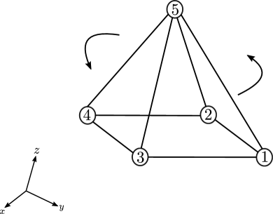
Figure 1: The actual formation, $\mathcal{G}(p)$, in $\mathbb{R}^{3}$.

We use an undirected graph topology to describe the interactions between these agents (see Figure 2). Accordingly, the neighbors sets are given as $\mathcal{N}_{1}=\{2\}$, $\mathcal{N}_{2}=\{1,3\}$, $\mathcal{N}_{3}=\{2,4\}$, $\mathcal{N}_{4}=\{3,5\}$ and $\mathcal{N}_{5}=\{4\}$.

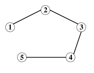
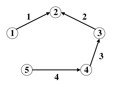
Figure 2: The interaction graph $\mathcal{G}$: (a) without an orientation (b) with an orientation.

To proceed with the first simulation, we assign an arbitrary orientation to the graph $\mathcal{G}$ as it is shown in Figure 2. The attitude initial conditions, for both schemes, are chosen as: $\hat{R}_{1}(0)=\mathcal{R}_{\alpha}(-\frac{\pi}{2},v)$, $\hat{R}_{2}(0)=\mathcal{R}_{\alpha}(\frac{\pi}{2},v)$, $\hat{R}_{3}(0)=\mathcal{R}_{\alpha}(-\frac{\pi}{2},v)$, $\hat{R}_{4}(0)=\mathcal{R}_{\alpha}(\frac{\pi}{2},v)$ and $\hat{R}_{5}(0)=\mathcal{R}_{\alpha}(-\frac{\pi}{2},v)$, with $v=[0~{}0~{}1]^{T}$. In addition, for Hybrid observer, we choose the following initial conditions for the auxiliary variables: $\xi_{k}(0)=0$ for every $k\in\{1,2,3,4\}$. Note that, according to these initial conditions, one has $\bar{R}_{k}(0)=\mathcal{R}_{\alpha}(\pi,v)$ and $\xi_{k}(0)=0$, $\forall k=\{1,2,3,4\}$, which implies that $x(0)\in\Upsilon\setminus\mathcal{A}$ and $x_{h}(0)\in\Upsilon_{h}\setminus\mathcal{A}_{h}$. Based on the parameters set $\mathcal{P}$, we select the following parameters: $\Xi=\{0.08\pi\}$, $A=\text{diag}([5,8.57,12])$, $\gamma=1.9251$, $\delta=0.0030$, $u=[0~{}0.6455~{}0.7638]^{T}$ and $\Delta^{*}=5$. For the gain parameters, we pick: $k_{R}=1.1$ and $k_{\xi}=5$. To simulate the Hybrid observer, we have used the HyEQ Toolbox [42].
Figure 3 and Figure 4 depict the time evolution of the relative attitude error norms $|\bar{R}_{k}(t)|_{I}$, for both schemes, and the auxiliary variables $\xi_{k}(t)$, $\forall k=\{1,2,3,4\}$, respectively, associated with each edge. Notice that, at $t=0$, the variables $\xi_{k}(t)$, $\forall k=\{1,2,3,4\}$, jump from $0$ to $0.08\pi$ and then converge to zero as $t\rightarrow\infty$. Also, the relative attitude error norms $|\bar{R}_{k}(t)|_{I}$, for both schemes, converge to zero as $t\rightarrow\infty$.

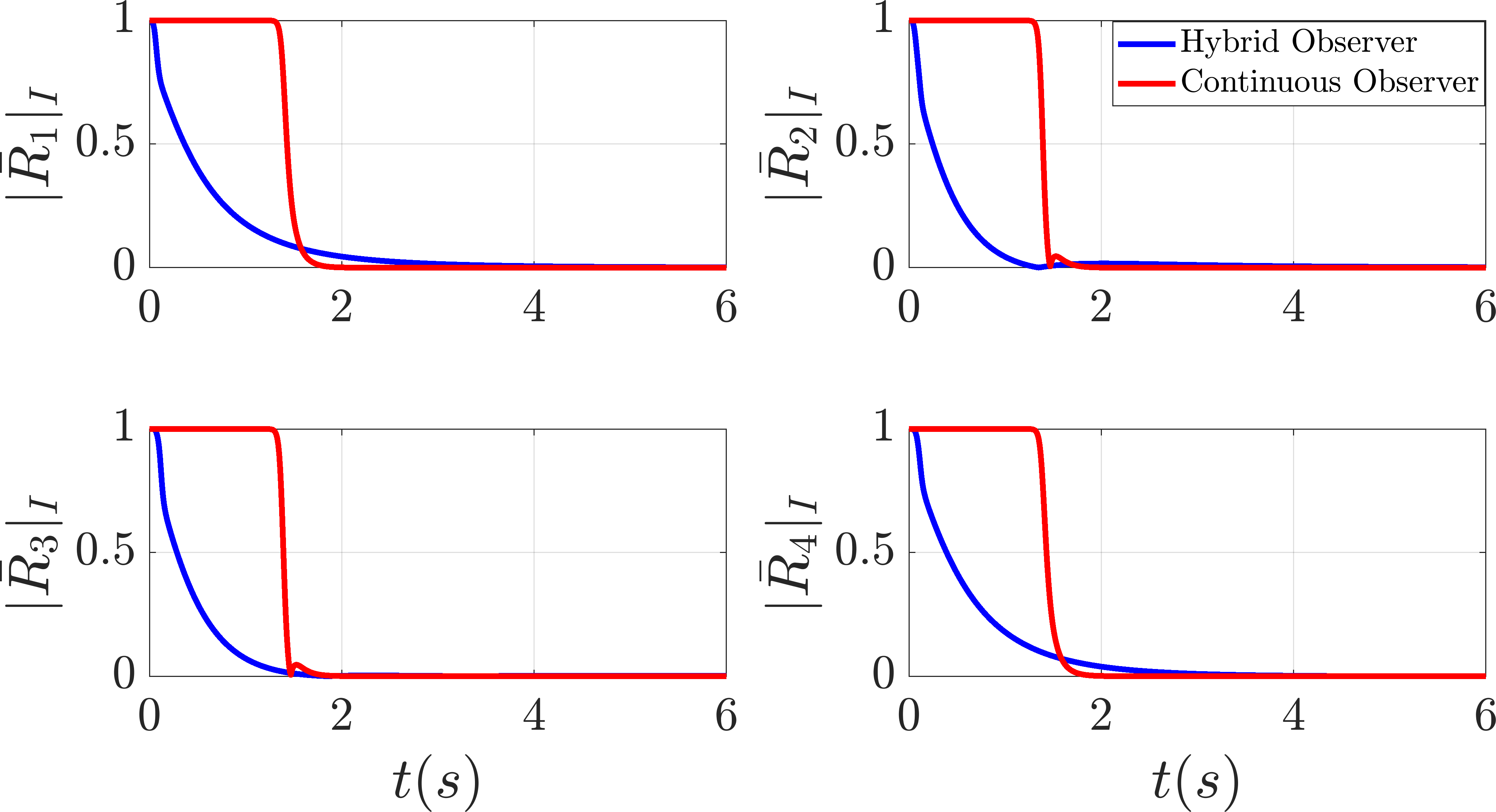
Figure 3: The time evolution of the relative attitude error norm, associated with each edge, for the Continuous observer and the Hybrid observer.

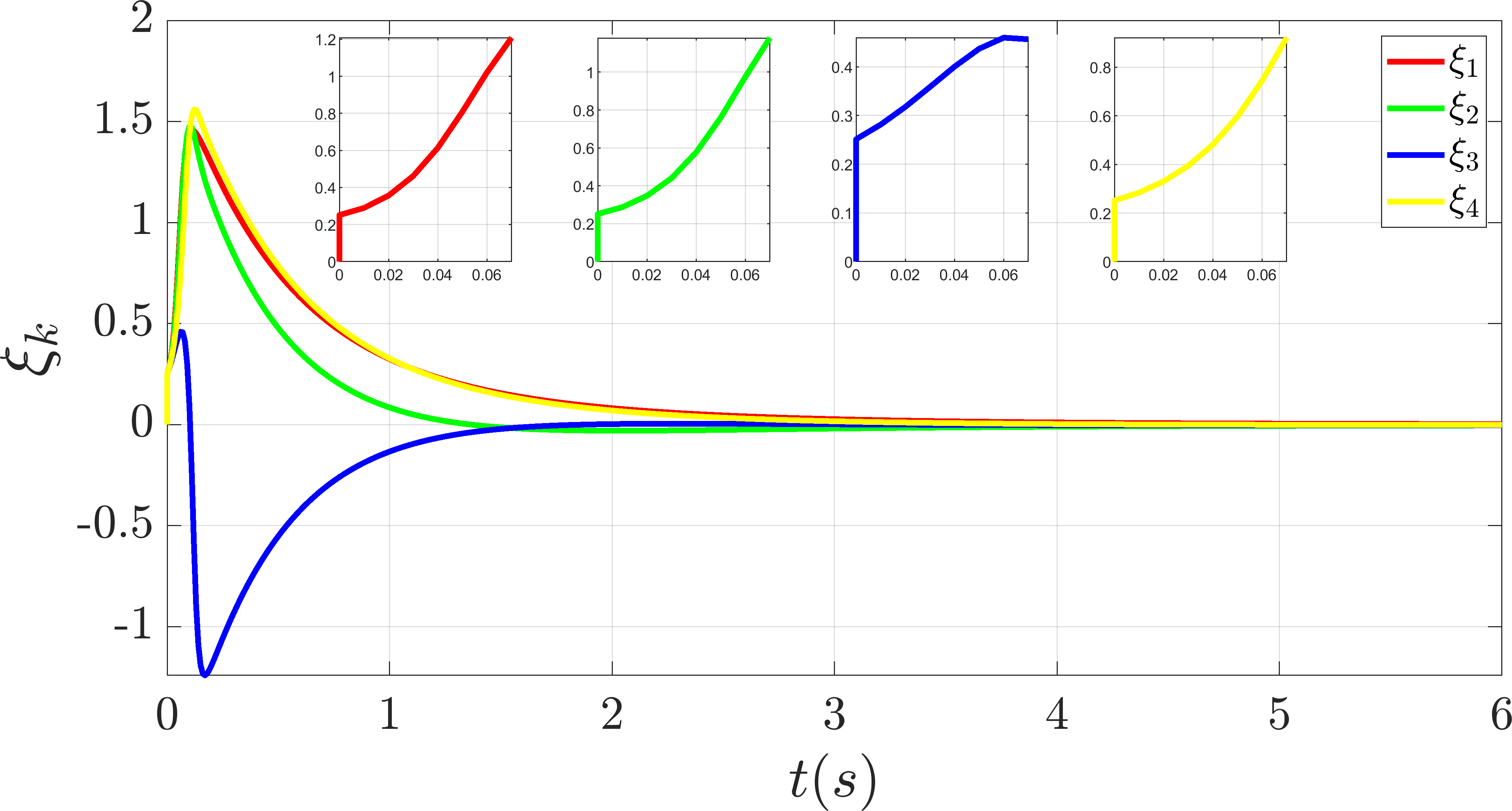
Figure 4: The time evolution of the hybrid variable $\xi_{k}$ associated with each edge.

In our second simulation, we simulate the proposed hybrid distributed position estimation scheme (57)-(58) together with the hybrid distributed attitude observer (52)-(53). We consider the following initial conditions for the estimated positions: $\hat{p}_{1}(0)=[1~{}1~{}0]^{T}$, $\hat{p}_{2}(0)=[-1~{}2~{}1]^{T}$, $\hat{p}_{3}(0)=[-2~{}0~{}-1]^{T}$, $\hat{p}_{4}(0)=[-1~{}2~{}2]^{T}$ and $\hat{p}_{5}(0)=[-1~{}1~{}1]^{T}$. We pick $k_{p}=1$. For the attitude observer (52)-(53), we consider the same initial conditions as in the first simulation.
The time evolution of the position and the relative position estimation error norms are provided in Figure 5 and Figure 6, respectively.

Figure 5: The time evolution of the position estimation error norm.

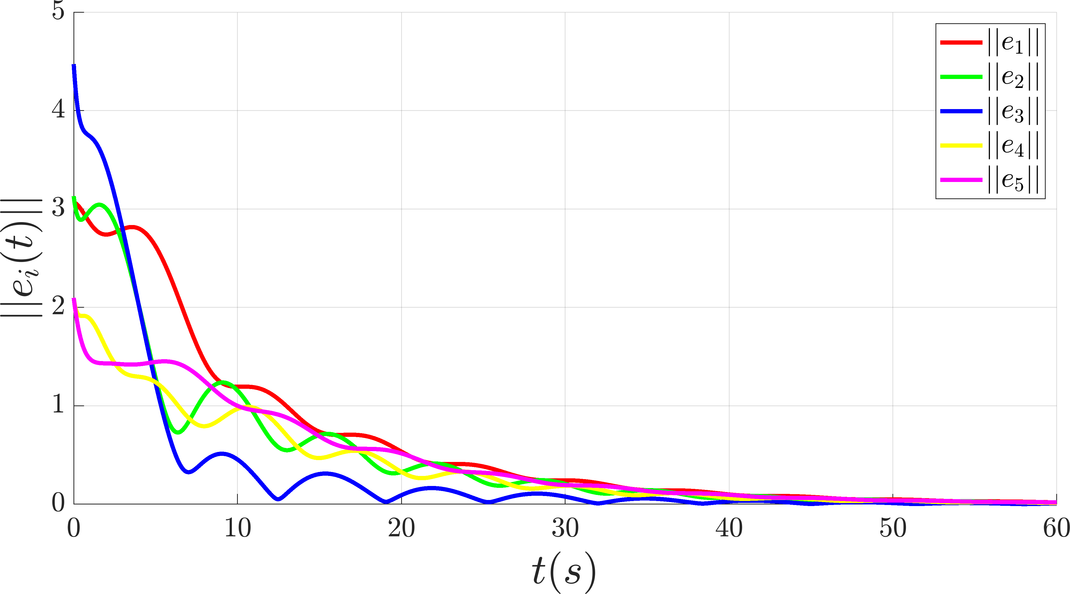
Figure 6: The time evolution of the relative position estimation error norm.

VII CONCLUSIONS

Two nonlinear distributed attitude estimation schemes have been proposed for multi-agent systems evolving on $SO(3)$. The first continuous observer, endowed with almost global asymptotic stability, is used as a baseline for the derivation of a stronger hybrid version enjoying global asymptotic stability of the desired equilibrium set $\mathcal{A}_{h}$, which implies that the attitude of each agent can be estimated (globally) up to a common constant orientation which can be uniquely determined if at least one agent has access to its absolute attitude. This hybrid distributed attitude estimation scheme relies on auxiliary time-varying scalar variables associated to each edge $k$, namely $\xi_{k}$, which are governed by the hybrid dynamics (34)-(35). These auxiliary variables are appropriately designed to keep the relative attitude errors away from the undesired equilibrium set $\Upsilon_{h}\setminus\mathcal{A}_{h}$ generated by smooth vector fields. Furthermore, the hybrid distributed attitude estimation scheme has been used with a hybrid distributed position estimation scheme to globally asymptotically estimate the pose of $N$ vehicles navigating in three-dimensional space, up to a constant translation and orientation, relying on local relative time-varying bearings between the agents, as well as the individual linear velocity measurements.
Note that our proposed estimation schemes rely on the assumption that the interaction graph topology is a tree (Assumption 2), which is practical in terms of communication and sensing costs. However, the main drawback of this graph topology is its vulnerability to failure since the failure of one agent will engender the disconnection of successive agents. Relaxing this assumption would be an interesting extension of this work.

References

• [1] M. Boughellaba and A. Tayebi, “Distributed hybrid attitude estimation for multi-agent systems on so(3),” in 2023 American Control Conference (ACC), 2023, pp. 1048–1053.
• [2] D. Koditschek, “The application of total energy as a lyapunov function for mechanical control systems,” Contemporary Mathematics, American Mathematical Society, 1989, vol. 97, 02 1989.
• [3] S. P. Bhat and D. S. Bernstein, “A topological obstruction to continuous global stabilization of rotational motion and the unwinding phenomenon,” Systems & Control Letters, vol. 39, no. 1, pp. 63–70, 2000.
• [4] R. Tron, B. Afsari, and R. Vidal, “Intrinsic consensus on so(3) with almost-global convergence,” in 2012 IEEE 51st IEEE Conference on Decision and Control (CDC), 2012, pp. 2052–2058.
• [5] ——, “Riemannian consensus for manifolds with bounded curvature,” IEEE Transactions on Automatic Control, vol. 58, no. 4, pp. 921–934, 2013.
• [6] J. Markdahl, “Synchronization on riemannian manifolds: Multiply connected implies multistable,” IEEE Transactions on Automatic Control, vol. 66, no. 9, pp. 4311–4318, 2021.
• [7] A. Sarlette, R. Sepulchre, and N. E. Leonard, “Autonomous rigid body attitude synchronization,” Automatica, vol. 45, no. 2, pp. 572–577, 2009.
• [8] ——, “Cooperative attitude synchronization in satellite swarms: A consensus approach,” IFAC Proceedings Volumes, vol. 40, no. 7, pp. 223–228, 2007, 17th IFAC Symposium on Automatic Control in Aerospace.
• [9] A. Sarlette and R. Sepulchre, “Consensus optimization on manifolds,” SIAM journal on control and optimization, vol. 48, no. 1, 2009.
• [10] R. Tron and R. Vidal, “Distributed 3-d localization of camera sensor networks from 2-d image measurements,” IEEE Transactions on Automatic Control, vol. 59, no. 12, pp. 3325–3340, 2014.
• [11] R. Tron, B. Afsari, and R. Vidal, “Average consensus on riemannian manifolds with bounded curvature,” in 2011 50th IEEE Conference on Decision and Control and European Control Conference, 2011, pp. 7855–7862.
• [12] B.-H. Lee and H.-S. Ahn, “Distributed estimation for the unknown orientation of the local reference frames in n-dimensional space,” in 2016 14th International Conference on Control, Automation, Robotics and Vision (ICARCV), 2016, pp. 1–6.
• [13] ——, “Distributed formation control via global orientation estimation,” Automatica, vol. 73, pp. 125–129, 2016.
• [14] Q. Van Tran, H.-S. Ahn, and B. D. O. Anderson, “Distributed orientation localization of multi-agent systems in 3-dimensional space with direction-only measurements,” in 2018 IEEE Conference on Decision and Control (CDC), 2018, pp. 2883–2889.
• [15] B.-H. Lee, S.-M. Kang, and H.-S. Ahn, “Distributed orientation estimation in so($d$) and applications to formation control and network localization,” IEEE Transactions on Control of Network Systems, vol. 6, no. 4, pp. 1302–1312, 2019.
• [16] Q. Van Tran, M. H. Trinh, D. Zelazo, D. Mukherjee, and H.-S. Ahn, “Finite-time bearing-only formation control via distributed global orientation estimation,” IEEE Transactions on Control of Network Systems, vol. 6, no. 2, pp. 702–712, 2019.
• [17] Q. Van Tran and H.-S. Ahn, “Distributed formation control of mobile agents via global orientation estimation,” IEEE Transactions on Control of Network Systems, vol. 7, no. 4, pp. 1654–1664, 2020.
• [18] X. Li, X. Luo, and S. Zhao, “Globally convergent distributed network localization using locally measured bearings,” IEEE Transactions on Control of Network Systems, vol. 7, no. 1, pp. 245–253, 2020.
• [19] A. Sarlette and R. Sepulchre, “Consensus optimization on manifolds,” SIAM Journal on Control and Optimization, vol. 48, no. 1, pp. 56–76, 2009.
• [20] P.-A. Absil, R. Mahony, and R. Sepulchre, Optimization Algorithms on Matrix Manifolds.   Princeton University Press, 2007.
• [21] W. Ren and R. W. Beard, Distributed Consensus in Multi-Vehicle Cooperative Control: Theory and Applications, 1st ed.   Springer Publishing Company, Incorporated, 2007.
• [22] H. Bai, M. Arcak, and J. T. Wen, “Rigid body attitude coordination without inertial frame information,” Automatica, vol. 44, no. 12, pp. 3170–3175, 2008.
• [23] R. Goebel and A. Teel, “Solutions to hybrid inclusions via set and graphical convergence with stability theory applications,” Automatica, vol. 42, no. 4, pp. 573–587, 2006.
• [24] R. Goebel, R. G. Sanfelice, and A. R. Teel, “Hybrid dynamical systems,” IEEE Control Systems Magazine, vol. 29, no. 2, pp. 28–93, 2009.
• [25] R. Goebel, R. Sanfelice, and A. Teel, Hybrid Dynamical Systems: Modeling, Stability, and Robustness.   Princeton University Press, 2012.
• [26] R. Mahony, T. Hamel, and J. Pflimlin, “Nonlinear complementary filters on the special orthogonal group,” IEEE Transactions on Automatic Control, vol. 53, no. 5, pp. 1203–1218, 2008.
• [27] M. Mesbahi and M. Egerstedt, Graph Theoretic Methods in Multiagent Networks.   Princeton: Princeton University Press, 2010.
• [28] Q. V. Tran, B. D. O. Anderson, and H.-S. Ahn, “Pose localization of leader-follower networks with direction measurements,” 2019.
• [29] L. Perko, Differential Equations and Dynamical Systems, 3rd ed.   Springer, 2000.
• [30] M. Morse, The calculus of variations in the large.   American Mathematical Soc, 1934, vol. 18.
• [31] C. G. Mayhew and A. R. Teel, “Synergistic potential functions for hybrid control of rigid-body attitude,” in Proceedings of the 2011 American Control Conference, 2011, pp. 875–880.
• [32] ——, “Hybrid control of rigid-body attitude with synergistic potential functions,” in Proceedings of the 2011 American Control Conference, 2011, pp. 287–292.
• [33] ——, “Synergistic hybrid feedback for global rigid-body attitude tracking on $so(3)$,” IEEE Transactions on Automatic Control, vol. 58, no. 11, pp. 2730–2742, 2013.
• [34] S. Berkane and A. Tayebi, “Construction of synergistic potential functions on so(3) with application to velocity-free hybrid attitude stabilization,” IEEE Transactions on Automatic Control, vol. 62, no. 1, pp. 495–501, 2017.
• [35] M. Wang and A. Tayebi, “Hybrid feedback for global tracking on matrix lie groups $so(3)$ and $se(3)$,” IEEE Transactions on Automatic Control, vol. 67, no. 6, pp. 2930–2945, 2022.
• [36] P. Casau, R. Cunha, R. G. Sanfelice, and C. Silvestre, “Hybrid control for robust and global tracking on smooth manifolds,” IEEE Transactions on Automatic Control, vol. 65, no. 5, pp. 1870–1885, 2020.
• [37] Z. Tang, R. Cunha, T. Hamel, and C. Silvestre, “Bearing-only formation control under persistence of excitation,” in 2020 59th IEEE Conference on Decision and Control (CDC), 2020, pp. 4011–4016.
• [38] A. Loria and E. Panteley, “Uniform exponential stability of linear time-varying systems: revisited,” Systems and Control Letters, vol. 47, no. 1, pp. 13–24, 2002.
• [39] H. Khalil, Nonlinear Systems, ser. Pearson Education.   Prentice Hall, 2002.
• [40] S. Zhao and D. Zelazo, “Localizability and distributed protocols for bearing-based network localization in arbitrary dimensions,” Automatica, vol. 69, pp. 334–341, 2016.
• [41] Z. Tang, R. Cunha, T. Hamel, and C. Silvestre, “Bearing leader-follower formation control under persistence of excitation,” IFAC-PapersOnLine, vol. 53, no. 2, pp. 5671–5676, 2020, 21st IFAC World Congress.
• [42] R. Sanfelice, D. Copp, and P. Nanez, “A toolbox for simulation of hybrid systems in matlab/simulink: Hybrid equations (hyeq) toolbox,” in Proceedings of the 16th International Conference on Hybrid Systems: Computation and Control, New York, USA, 2013, p. 101–106.