Individual Welfare Analysis: Random Quasilinear Utility, Independence, and Confidence Bounds

We introduce a novel framework for individual-level welfare analysis. It builds on a parametric model for continuous demand with a quasilinear utility function, allowing for heterogeneous coefficients and unobserved individual-product-level preference shocks. We obtain bounds on the individual-level consumer welfare loss at any confidence level due to a hypothetical price increase, solving a scalable optimization problem constrained by a new confidence set under an independence restriction. This confidence set is computationally simple, robust to weak instruments, nonlinearity, and partial identification. In addition, it may have applications beyond welfare analysis. Monte Carlo simulations and two empirical applications on gasoline and food demand demonstrate the effectiveness of our method.

Keywords: Welfare analysis, nonlinear models, inferential method, independence.

JEL Codes: C12, C20, C50, D12

1 Introduction

Consumer welfare analysis is an important topic in microeconomics. However, commonly adopted methods for welfare analysis are typically at the aggregated or averaged level, unable to recover individual heterogeneity. This paper proposes a novel framework to conduct individual-level welfare inference under a simple demand model. More specifically, we aim to obtain confidence bounds on the welfare loss under a hypothetical price increase for an individual whose consumption level before the price hike is pre-specified.

Our framework builds on a parametric model for continuous demand following Brown and Calsamiglia (2007) and Brown, Deb and Wegkamp (2007). The model has a quasilinear utility function that allows for multiple goods and unobservables. Structural parameters in the model can depend on observables such as income or can be individual-specific. We derive the welfare loss under a price increase as a function of the parameters. Suppose we have a $(1-\alpha)\in(0,1)$ confidence set for these parameters. We can then infer the maximum and minimum of the welfare loss with confidence $(1-\alpha)$ by solving an optimization problem constrained by the confidence set. We show that under the chosen utility function, the welfare loss function is strictly increasing in each parameter, so the welfare loss bounds are very easy to obtain. Moreover, the function is also concave in the parameters. Therefore, if a researcher wishes to impose additional convex constraints on the parameters, the maximal welfare loss bound can still be computed quickly even for each individual in the sample with a large number of goods.

Individual-level welfare bounds provide a deeper understanding of the data as they allow for the examination of heterogeneity within the data. Unlike a point counterfactual estimate, which is commonly produced through econometric procedures in structural modeling, our bounds are designed to incorporate a specified level of confidence. This means that there is no need for any additional computationally intensive inferential procedures to be conducted at the individual level.

To implement the method, we need to first obtain a confidence set at the desired confidence level for the structural parameters. We propose a new confidence set under independence. The set is constructed by inverting a recently developed statistic that measures the dependence between two random variables by Chatterjee (2021). Unlike the traditional Kolmogorov-Smirnov- or the Cramér-von Mises-criterion-based inferential methods under independence, our new confidence set can be easily computed without the need for numerical integration or parameter tuning. Its theoretical validity is derived without high level technical conditions. It is also robust to nonlinearity in the parameters and to weak instruments. This method is of independent interest and can have other applications in different areas in economics.

To obtain tight bounds on welfare loss, it is desirable to have a tight confidence set as the constraints. Our proposed confidence set, which is similar to the inversion of the Anderson-Rubin statistic, may not always be bounded. To overcome this issue, we can intersect our confidence set with another set obtained through alternative methods, with Bonferroni correction. In our demand model, we can construct a confidence interval for each parameter through 2SLS or OLS, and by applying nonlinear transformations, such as the delta method. However, due to the nonlinear nature of the model, this alternative confidence interval may be wide. By intersecting the two confidence intervals, we can tighten the confidence set, as observed in our empirical applications even with a small sample size despite the potential conservativeness of Bonferroni correction.

There is a large literature on demand estimation. See Dubé (2019) for a review of recent developments. The typical approach constructs a plug-in estimator of welfare change using a point-estimator of the parameters of a structural model. However, usually there is no corresponding confidence interval for the welfare analysis. For estimation and inferential methods under independence, perhaps the most popular approach is to exploit the relationship between the joint and marginal distributions of the exogenous variable and unobservable. In his pioneering work, Manski (1983) proposes an estimation strategy that minimizes the mean square distance between these distributions. Brown and Wegkamp (2002), Brown, Deb and Wegkamp (2007), Komunjer and Santos (2010), and Torgovitsky (2017) extend the approach to more flexible model setups. These approaches would be computationally challenging as they require estimating cumulative distribution functions or moment generating functions at many points and computing the Cramér-von Mises criterion numerically. Poirier (2017) minimizes the mean square distance between the conditional and marginal densities. The approach requires the practitioners to choose basis functions and their dimensions even for parametric models. Selecting these tuning parameters creates hurdles in implementation, and different choices may affect the finite sample performance of the estimator. Our inferential method, in contrast, is free of tuning parameters.

The rest of the paper is organized as follows. Section 2 sets up the demand model and develops our framework of inferring the bounds on the welfare loss with confidence. Section 3 proposes a new method to construct confidence sets under independence. Section 4 presents Monte Carlo simulations. Section 5 demonstrates two empirical examples on gasoline and food demand. The Appendices provide heuristics on the shape and size of our confidence set and implementation details and some extensions.

2 Individual-Level Welfare Confidence Bounds

We consider the demand model in Brown, Deb and Wegkamp (2007) (henceforth BDW for simplicity). Suppose there are $K>0$ goods. For $k=1,\ldots,K$, let $Y_{k}$ and $P_{k}$ be the consumption and price of good $k$, respectively. Let $Y_{0}$ be the numéraire good with $P_{0}=1$. Let $W_{k}$ be an unobserved nonnegative random variable that affects the consumer’s utility for good $k$. Let the $K\times 1$ vectors $\bm{Y},\bm{P}$ and $\bm{W}$ collect $Y_{k}$, $P_{k}$ and $W_{k}$ for $k=1,\ldots,K$ respectively. For a consumer with income level $I$, she maximizes her quasilinear log utility $U(Y_{0},\bm{Y},\bm{W},\theta)$ subject to the budget constraint:

$$\max_{Y_{0},\bm{Y}}\ \ U(Y_{0},\bm{Y},\bm{W},\bm{\theta})\coloneqq Y_{0}+U_{0}\left(\bm{Y};\bm{\theta}\right)+\bm{W}^{\prime}\bm{Y}$$

$$= Y_{0}+\sum_{k=1}^{K}\theta_{k}g_{k}(Y_{k})+\bm{W}^{\prime}\bm{Y}$$ (2.1)

$$s.t.\ \ Y_{0}+\bm{P}^{\prime}\bm{Y}=I,$$ (2.2)

where $\bm{\theta}\coloneqq(\theta_{k})\in(0,1)^{K}$. The function $g_{k}$ is a known concave and strictly increasing function for all $k$.

For concreteness, let $g_{k}=\log(\cdot)$ for each $k$; this is the case when the utility is Cobb-Douglas; BDW adopts this functional form as the leading example. We also allow $U_{0}$ to take other functional forms, or in principle allow $\bm{W}$ to enter $U_{0}$. We provide more details on these extensions in Appendix C and Remark 2.5.

On the other hand, we maintain linearity in $Y_{0}$ even in those extensions. Such linearity makes the utility we consider a special case of a random quasilinear utility function proposed by Brown and Calsamiglia (2007) that develops theoretical results for quasilinear rationalizations of consumer demand data. Under a quasilinear utility function, welfare changes due to a shift in price can be measured by changes in consumer surplus, which is in turn the difference in the indirect utility function at the old and new prices. This property is useful to gain computational efficiency for the empirical method we propose.

One major limitation of quasilinearity utility is the absence of the income effect. We can mitigate this by allowing $\bm{\theta}$ to depend on income groups so that the income effect can still be present. We consider such a model in our first empirical application in Section 5.1. Alternatively, when a panel data set is available, we can allow $\bm{\theta}$ to differ across individuals but constant across time. In this case, individual-wise income effect can exist; we consider this model in the second empirical application in Section 5.2.

Assuming an interior solution, BDW derives the following first order condition for the optimal consumption $\bm{Y}^{*}(\bm{P},\bm{W};\bm{\theta})$:

$$W_{k}=P_{k}-\frac{\theta_{k}}{Y_{k}^{*}(\bm{P},\bm{W};\bm{\theta})},\;k=1,\ldots,K.$$ (2.3)

The model (C) captures product-specific consumer heterogeneity in the sense that it allows for an unobserved preference shock $W_{k}$ for each product $k$. Furthermore, the model exploits separability, so that the first order condition for each product $k$ only involves its own $(W_{k},P_{k},\theta_{k},Y^{*}_{k})$ elements but not those from other products. It follows from (2.3) that the demand for good $k$ is explicitly written as

$$Y_{k}^{*}(\bm{P},\bm{W};\bm{\theta})=\frac{\theta_{k}}{P_{k}-W_{k}}.$$ (2.4)

Substituting the budget constraint (2.2) and the optimal demand (2.4), we then obtain the following indirect utility function from (C):

$$V(I,\bm{P},\bm{W},\bm{\theta}):=I+\sum_{k=1}^{K}\theta_{k}\log\frac{\theta_{k}}{(P_{k}-W_{k})}-\sum_{k=1}^{K}\theta_{k}.$$ (2.5)

We now focus on a change in consumer welfare due to a change in prices, measured by consumer surplus. Let $\bar{\bm{w}}$ be a vector of realized $\bm{W}$ and ($\bm{p}^{0}$, $\bm{p}^{1}$) be two price levels; neither $\bm{p}^{0}$ nor $\bm{p}^{1}$ needs to be the actual observed price. Denote the optimal consumption under $\bm{p}^{j}$ and $\bar{\bm{w}}$ by $\bm{y}^{j}$; that is, $\bm{y}^{j}\coloneqq\bm{Y}^{*}(\bm{p}^{j},\bar{\bm{w}};\bm{\theta})$, $j=0,1$. Assume that $\bar{\bm{w}}$ is smaller than both $\bm{p}^{0}$ and $\bm{p}^{1}$ so that the optimal consumption levels are interior solutions. This assumption is automatically satisfied if $\bm{y}^{0}>\bm{0}$ and $\bm{p}^{1}\geq\bm{p}^{0}$; see Remark 2.2 for details. Let $\bm{\Delta}:=\bm{p}^{1}-\bm{p}^{0}$ be the vector of price changes. By the definition of $\bm{y}^{0}$ and $\bm{y}^{1}$, equation (2.5) implies that the welfare loss denoted by $\text{WL}(\bm{\theta})$, when the price changes from $\bm{p}^{0}$ to $\bm{p}^{1}$ while $\bm{W}$ is fixed at $\bar{\bm{w}}$, is as follows:

$$\mathrm{WL}(\bm{\theta}) \coloneqq V(I,\bm{p}^{0},\bar{\bm{w}},\bm{\theta})-V(I,\bm{p}^{1},\bar{\bm{w}},\bm{\theta})$$

$$=\sum_{k=1}^{K}\theta_{k}\log\left[\frac{p_{k}^{1}-\bar{w}_{k}}{p_{k}^{0}-\bar{w}_{k}}\right]$$

$$=\sum_{k=1}^{K}\theta_{k}\log\left[1+\frac{\Delta_{k}y_{k}^{0}}{\theta_{k}}\right].$$ (2.6)

Hence, the welfare loss solely depends on $\bm{y}^{0}$, the price change $\bm{\Delta}$, and the unknown parameters $\bm{\theta}$.

Remark 2.1.

It is known that under the standard Cobb-Douglas preference, the optimal consumption is always an interior positive solution to the optimization problem (C)-(2.2). With the presence of the positive unobserved $\bm{W}$, the model is able to generate corner solutions, fitting real data better. A corner solution occurs when $W_{k}>P_{k}$. In this case, since we cannot write down a reduced form which expresses $\bm{W}$ as a function of the observables and parameters, we cannot form moment conditions for the parameters. This phenomenon exists regardless of the functional form of $U_{0}$ in equation (C). We focus on interior solutions throughout the paper and leave the study of corner solutions to future research.

Remark 2.2.

For simplicity, we only focus on a price increase in this paper, i.e., $\Delta_{k}\geq 0$ for all $k>0$, but in fact we can analyze the welfare change under a price decrease as well so long as the optimal consumption at the new price is still an interior solution. By equation (2.3), setting $\bm{y}^{0}>\bm{0}$ implicitly sets $\bm{p}^{0}>\bar{\bm{w}}$ since $p^{0}_{k}-\bar{w}_{k}=\theta_{k}/y_{k}^{0}$ for all $k$. Therefore, when considering a price change $\Delta_{k}=p^{1}_{k}-p^{0}_{k}$, the interior solution requirement $p^{1}_{k}-\bar{w}_{k}>0$ implies $\Delta_{k}+p_{k}^{0}-\bar{w}_{k}>0$, which leads to $\Delta_{k}>-\theta_{k}/y_{k}^{0}$; this is exactly the condition that makes the right hand side of equation (2.6) well-defined. This inequality is satisfied when $\Delta_{k}>0$. For a price drop ($\Delta_{k}<0$), once we obtain a confidence set of $\theta_{k}$ with its lower bound $\hat{L}_{k}>0$, we can compute the welfare loss bounds under $\Delta_{k}$ as long as $\Delta_{k}>-\hat{L}_{k}/y^{0}_{k}$.

Remark 2.3.

All the prices $P_{k}$ in the derivation of the indirect utility and welfare change are real prices by normalizing the price of the numéraire to be 1. In most applications, however, real prices are infeasible since we can only observe nominal prices in data. Denoting the nominal price for good $k=0,\ldots,K$ by $P_{k}^{n}$, we have $P^{n}_{k}/P_{k}\equiv P^{n}_{0}/1$ for every $k$. Equation (2.3) written in terms of the nominal prices then becomes $P_{k}^{n}-P_{0}^{n}W_{k}=P^{n}_{0}\theta_{k}/Y_{k}$. Since we only observe $P_{k}^{n}$ and $Y_{k}$ in data, we can only treat $P_{0}^{n}W_{k}$ as the unobservable and $P^{n}_{0}\theta_{k}$ as the parameter. Consequently, although the real $\theta_{k}$ is assumed to lie in $(0,1)$ by BDW, we do not restrict the confidence interval to be upper bounded by 1 in the empirical applications: The parameter that data can recover is $P^{n}_{0}$ times of the real $\bm{\theta}$ and $P^{n}_{0}$ is unknown. With a bit abuse of notation, in the rest of the paper, we still denote the nominal price $P^{n}_{k}$ and the parameter $P^{n}_{0}\theta_{k}$ by $P_{k}$ and $\theta_{k}$ respectively for simplicity.

2.1 Predicting the Individual Welfare Loss Bounds with Confidence

Suppose that we have micro-level i.i.d. data on $\{(P_{k,i},Y_{k,i},{\bm{X}_{i}}):i=1,\ldots,n_{k};k=1,\ldots,K\}$, where subscript $i$ refers to observation $i$. Vector $\bm{X}_{i}$ contains other observables in the data. For a given price change $\bm{\Delta}$ and consumption level $\bm{y}^{0}$, it remains to deal with the unknown $\bm{\theta}$ to compute the welfare change. In principle, we allow $\bm{\theta}$ to depend on $i$ as long as it can be identified; each $\theta_{k}$ can be either a nonparametric function of the other observables $\bm{X}_{i}$, or contain $i$-specific fixed coefficients. In our empirical applications, the varying coefficient model in Section 5.1 and the model in Section 5.2 follow these two setups respectively. For notational simplicity, we treat $\bm{\theta}$ as homogeneous across $i$ in this section and in Section 3.

For a given $\alpha\in(0,1)$, assume that we have a $(1-\alpha/K)$ confidence interval for each $\theta_{k}$: $[\hat{L}_{k}(1-\alpha/K),\hat{U}_{k}(1-\alpha/K)]$. We can then construct a $(1-\alpha)$ box confidence set by Bonferroni correction: $\Pr(\bm{\theta}\in\prod_{k=1}^{K}[\hat{L}_{k}(1-\alpha/K),\hat{U}_{k}(1-\alpha/K)])\geq 1-\alpha$. Although Bonferroni correction may not be efficient, it is very simple and computationally straightforward.

Remark 2.4.

Theory-wise, even if the number of goods $K$ is large, the sample size $n_{k}$ can be relatively small for each $k$ because we can obtain the confidence intervals for each $\theta_{k}$ separately only using the data for good $k$.

We can then predict the maximal and minimal welfare loss with confidence $(1-\alpha)$ for an individual with consumption $\bm{y}^{0}\equiv\{y^{0}_{1},\ldots,y^{0}_{K}\}$ due to a price change $\bm{\Delta}\equiv(\Delta_{1},\ldots,\Delta_{K})$. Using the maximum as an example, we solve the following problem:

$$\max_{\tilde{\bm{\theta}}} \ \ \sum_{k=1}^{K}\tilde{\theta}_{k}\log\left[1+\frac{\Delta_{k}}{\tilde{\theta}_{k}}{y_{k}^{0}}\right],$$

$$s.t. \ \ \hat{L}_{k}(1-\alpha/K)\leq\tilde{\theta}_{k}\leq\hat{U}_{k}(1-\alpha/K),0\leq\tilde{\theta}_{k},\forall k=1,\ldots,K.$$

Theorem 2.1.

Let the maximum of the objective function under the constraint above be $\widehat{\mathrm{WL}}^{*}$. For each $k=1,\ldots,K$, if $\Pr(\hat{L}_{k}(1-\alpha/K)\leq\theta_{k}\leq\hat{U}_{k}(1-\alpha/K))\to(1-\alpha/K)$ with the sample size $n_{k}\to\infty$, then

$$\lim_{n_{k}\to\infty,k=1,\ldots,K}\Pr(\mathrm{WL}(\bm{\theta})\leq\widehat{\mathrm{WL}}^{*})\geq(1-\alpha).$$

Proof.

By construction, the event $\{\mathrm{WL}(\bm{\theta})\leq\widehat{\mathrm{WL}}^{*}\}$ happens as long as $\hat{L}_{k}(1-\alpha/K)\leq\theta_{k}\leq\hat{U}_{k}(1-\alpha/K)$ for all $k$. Therefore,

$$\lim_{\begin{subarray}{c}n_{k}\to\infty\\ k=1,\ldots,K\end{subarray}}\Pr\left(\mathrm{WL}(\bm{\theta})\leq\widehat{\mathrm{WL}}^{*}\right)$$

$$\geq \lim_{\begin{subarray}{c}n_{k}\to\infty\\ k=1,\ldots,K\end{subarray}}\Pr\left(\hat{L}_{k}(1-\alpha/K)\leq\theta_{k}\leq\hat{U}_{k}(1-\alpha/K),\forall k\right)$$

$$\geq 1-K\cdot\frac{\alpha}{K}$$

$$= 1-\alpha,$$

where the second inequality is by the union bound. ∎

Individual-level welfare bounds contain more information than a bound at the aggregated level; one can view and study the heterogeneity from them. Moreover, our bound is different from a point estimate; it by construction incorporates the desired confidence level, so no further inferential procedure is needed.

Remark 2.5.

Because the model is separable in $\bm{W}$, the heterogeneous realization of $\bm{W}$ across individuals does not affect the welfare change once $\bm{y}_{0}$ and $\bm{\Delta}$ are fixed. To capture individual heterogeneity, $\bm{y}_{0}$ can be the realized consumption of each individual. Moreover, as discussed before, we can allow $\bm{\theta}$ to differ across individuals as well so long as the data have sufficient variation to identify it. Our empirical applications in Section 5 provide such examples. Alternatively, we can accommodate a model that is nonseparable in $\bm{W}$. In that case, the welfare change function in general depends on the realization of $\bm{W}$, inducing individual heterogeneity. One can either set $\bm{W}$ to be a counterfactual value or use its actual realization in a data set, backed out using the observed consumption and price.

For the optimization problem, as we show in Appendix B, the welfare loss function is strictly increasing in each $\theta_{k}$ when $\theta_{k}>0$ and $\Delta_{k}y_{k}^{0}>0$. One can thus easily obtain the maximum and minimum of the welfare loss by substituting all the upper and lower bounds on the $\theta_{k}$s, respectively. When there are additional convex constraints besides the confidence intervals, for instance, $\sum_{k=1}^{K}\tilde{\theta}_{k}=1$, one can still solve the maximization problem quickly by off-the-shelf convex optimization algorithms because the objective function is concave in $\bm{\theta}$; see Appendix B.2 for more details.

3 A New Confidence Set for Nonlinear Models

So far, we have assumed the existence of a confidence interval for each $\theta_{k}$. In this section, we introduce a novel approach to obtain it. This approach is based on a new correlation coefficient to measure independence developed by Chatterjee (2021). We first briefly review this statistic for completeness.

Consider an i.i.d. sample $\{(R^{(1)}_{i},R^{(2)}_{i}):i=1,\ldots,n\}$ for random variables $R^{(1)}$ and $R^{(2)}$. Suppose that the $R^{(1)}_{i}$s and $R^{(2)}_{i}$s have no ties. Sort the data by $R^{(1)}$ in ascending order. Let the rearranged data be $(R^{(1)}_{(1)},R^{(2)}_{(1)}),\ldots,(R^{(1)}_{(n)},R^{(2)}_{(n)})$ where $R^{(1)}_{(1)}<\cdots<R^{(1)}_{(n)}$. Let $r_{i}$ be the rank of $R^{(2)}_{(i)}$. Chatterjee (2021) proposes the following statistic to measure the dependence between $R^{(1)}$ and $R^{(2)}$:

$$\xi_{n}(R^{(1)},R^{(2)})\coloneqq 1-\frac{3\sum_{i=1}^{n-1}|r_{i+1}-r_{i}|}{n^{2}-1}.$$ (3.1)

When $R^{(1)}\perp R^{(2)}$, where $\perp$ denotes independence, Chatterjee shows in Theorem 1.1 that $\xi_{n}(R^{(1)},R^{(2)})\overset{p}{\to}0$. Meanwhile, $R^{(1)}\not\perp R^{(2)}$ if and only if $\text{plim }\xi_{n}(R^{(1)},R^{(2)})>0$. Moreover, under $R^{(1)}\perp R^{(2)}$, his Theorem 2.2 shows that

$$\sqrt{n}\xi_{n}(R^{(1)},R^{(2)})\overset{d}{\to}N(0,\tau^{2}),$$

where $\tau^{2}=0.4$ if $R^{(2)}$ is continuous. When $R^{(2)}$ is discrete, $\tau^{2}$ can be consistently estimated by

$$\hat{\tau}_{n}=\sqrt{\frac{a_{n}-2b_{n}+c_{n}^{2}}{d_{n}^{2}}},$$ (3.2)

where by letting $\mathcal{R}(i)\coloneqq\#\{j:R^{(2)}_{j}\leq R^{(2)}_{i}\}$, $\mathcal{L}(i)\coloneqq\#\{j:R^{(2)}_{j}\geq R^{(2)}_{i}\}$, $u_{1}\leq\cdots\leq u_{n}$ be an increasing rearrangement of $\mathcal{R}(i)$ and $v_{i}\coloneqq\sum_{j=1}^{i}u_{j}$ for all $i$, Chatterjee defines

$$a_{n}\coloneqq \frac{1}{n^{4}}\sum_{i=1}^{n}\left(2n-2i+1\right)u_{i}^{2},\ \ \ \ b_{n}\coloneqq\frac{1}{n^{5}}\sum_{i=1}^{n}\left(v_{i}+(n-i)u_{i}\right)^{2},$$

$$c_{n}\coloneqq \frac{1}{n^{3}}\sum_{i=1}^{n}\left(2n-2i+1\right)u_{i},\ \ \ \ d_{n}\coloneqq\frac{1}{n^{3}}\sum_{i=1}^{n}\mathcal{L}(i)\left(n-\mathcal{L}(i)\right).$$

Chatterjee notes in his Theorem 2.3 that $\hat{\tau}_{n}^{2}$ can be computed in time $O(n\log(n))$.

Now we introduce our new confidence sets for the $\theta_{k}$s. For $k=1,\ldots,K$, let $Z_{k}$ be an observed random variable such that $W_{k}\perp Z_{k}$. Depending on applications, this $Z_{k}$ can be price itself or its instrumental variable. Although the independence assumption is strong, it is indispensable in many nonseparable models, which we could handle as mentioned in Remark 2.5. Let $c_{1-\alpha}\coloneqq\hat{\tau}_{n}z_{1-\alpha}$ where $z_{1-\alpha}$ is the $(1-\alpha)$-th quantile of the standard normal distribution. $\hat{\tau}_{n}=\sqrt{0.4}$ if $Z_{k}$ is continuous, and follows (3.2) by treating $Z_{k}$ as $R^{(2)}$ if $Z_{k}$ is discrete. For simplicity, assume that $n_{k}=n$ for all $k$. For any $\alpha\in(0,1)$, we construct a $(1-\alpha)$ confidence set by inverting Chatterjee’s statistic:

$$CS^{\xi}_{k}(1-\alpha)\coloneqq\{\theta\in\Theta_{k}:\xi_{n}(P_{k}-\theta/Y_{k},Z_{k})\leq c_{1-\alpha}/\sqrt{n}\},$$ (3.3)

where $\Theta_{k}$ is the parameter space of $\theta_{k}$.

Theorem 3.1.

Suppose that an i.i.d. sample of $\{(P_{k,i},Y_{k,i},Z_{k,i}):i=1,\ldots,n;k=1,\ldots,K\}$ is used to obtain $\xi_{n}(P_{k}-\theta/Y_{k},Z_{k})$. For each $k$, if $W_{k}\perp Z_{k}$, then under the first order condition (2.3), as the sample size $n\rightarrow\infty$, $\Pr(\theta_{k}\in CS^{\xi}_{k}(1-\alpha))\to 1-\alpha$ for any $\alpha\in(0,1)$.

Proof.

By equation (2.3) and $Z_{k}\perp W_{k}$, we have $(P_{k}-\theta_{k}/Y_{k})\perp Z_{k}$. Hence, by i.i.d. and by Theorems 2.2 and 2.3 in Chatterjee (2021), we have $\sqrt{n}\xi_{n}(P_{k}-\theta_{k}/Y_{k},Z_{k})/\hat{\tau}_{n}\overset{d}{\to}N(0,1)$. Therefore, $\Pr(\sqrt{n}\xi_{n}(P_{k}-\theta_{k}/Y_{k},Z_{k})/\hat{\tau}_{n}\leq z_{1-\alpha})\to 1-\alpha$. The desired result is obtained by substituting the definition of $CS^{\xi}_{k}(1-\alpha)$. ∎

Remark 3.1.

This new inferential method is computationally fast. As discussed by Chatterjee (2021), $\xi_{n}$ can be computed in $O(n\log n)$ time regardless of the continuity of data. For $\hat{\tau}_{n}$, it is a known constant for a continuous $Z_{k}$, and can also be computed in time $O(n\log n)$ if $Z_{k}$ is discrete. As $\theta_{k}$ is a scalar, we can obtain the confidence set easily by grid search. During the searching process, $\hat{\tau}_{n}$ for a discrete $Z_{k}$ only needs to be computed once because it does not depend on the unknown parameter.

It is important to note that Theorem 3.1 does not require any relevance condition. Validity of the confidence set holds regardless of the strength of the instrument. Even if the model is only partially identified or the instrument is weak, $CS_{k}^{\xi}(1-\alpha)$ always yields the correct asymptotic coverage probability for the true parameter. Moreover, one does not need to distinguish the point and partially identified cases. On the other hand, the strength of the instrument does affect the length of the confidence set. For instance, if $Z_{k}$ is independent of both $P_{k}$ and $W_{k}$, then one can see that $CS^{\xi}_{k}(1-\alpha)$ can be the entire real line. Appendix A provides more details on the shape and size of the confidence set.

One possible drawback of Chatterjee’s test of independence is its low power (Shi, Drton and Han, 2022), which may result in a wide confidence set. Shi, Drton and Han (2022) show that there are alternative statistics for independence that have better power properties, such as the Hoeffding’s $D$ (Hoeffding, 1948), Bergsma-Dassios-Yanagimoto’s $\tau^{*}$ (Bergsma and Dassios, 2014; Yanagimoto, 1970) and Blum-Kiefer-Rosenblatt’s $R$ (Blum, Kiefer and Rosenblatt, 1961). However, when the instrument is discrete, computing $\tau^{*}$ and $R$ for each candidate value of the parameter takes at least $O(n^{2})$ time (see Shi, Drton and Han (2022) and the references therein). Meanwhile, all the three alternative statistics, under independence, have nonstandard limiting distributions, especially when the instrument is discrete (Shi, Drton and Han, 2022; Nandy, Weihs and Drton, 2016), making it harder to get a confidence set than inverting Chatterjee’s statistic.

To mitigate the low power problem and tighten the confidence set, we propose the following intersection approach by intersecting our confidence set with another one obtained by alternative methods.

3.1 Intersecting Confidence Sets

For the demand model we consider, rearranging equation (2.3), we have $1/Y_{k}=\beta_{k}P_{k}-\beta_{k}W_{k}$ where $\beta_{k}=1/\theta_{k}$. Treating $1/Y_{k}$ as the dependent variable, we can estimate $\beta_{k}$ by OLS or 2SLS and obtain a confidence interval for $\theta_{k}$ by, for instance, the delta method. If a weak instrument is concerned, one could use an Anderson-Rubin-type confidence interval. Let the $(1-\alpha/K)$ confidence interval obtained in this way be $CS^{LS}_{k}(1-\alpha/K)$.

Since $CS^{\xi}_{k}$ and $CS^{LS}_{k}$ utilize information differently, it is possible that neither is a subset of the other. We can construct $\hat{L}_{k}(1-\alpha/K)$ and $\hat{U}_{k}(1-\alpha/K)$ for each $k$ by taking the minimum and maximum of $CS^{\xi}_{k}(1-\alpha/2K)\cap CS^{LS}_{k}(1-\alpha/2K)$, respectively, to sharpen the confidence set. Note that the confidence level for each confidence set is $(1-\alpha/2K)$ to implement the Bonferroni correction. In our empirical applications, we do observe improvement in this intersection approach compared to using one method alone.

Furthermore, the intersection approach also improves feasibility in computing the $CS^{\xi}_{k}$s. As we propose to compute $CS^{\xi}_{k}$ by grid search, a parameter space for $\theta_{k}$ is needed. However, the upper bound on $\theta_{k}$ is usually unknown in practice; see Remark 2.3 for details. Now the bounded $CS^{LS}_{k}(1-\alpha/2K)$ can serve as the parameter space by noting that

$$CS^{\xi}_{k}(1-\alpha/2K)\cap CS^{LS}_{k}(1-\alpha/2K)$$

$$= \{\theta\in CS^{LS}_{k}(1-\alpha/2K):\sqrt{n}\xi_{n}(P_{k}-\theta/Y_{k},Z_{k})\leq c_{1-\alpha/2K}\}.$$

Therefore, we can obtain $CS^{\xi}_{k}(1-\alpha/2K)\cap CS^{LS}_{k}(1-\alpha/2K)$ using grid search within $CS^{LS}_{k}(1-\alpha/2K)$.

4 Monte Carlo Simulations

4.1 A Three-Goods Economy

In this section, we simulate a model with three goods. The confidence sets are obtained by using the $CS_{k}^{\xi}$s alone. We examine the performance of both the confidence set and the upper bound on welfare loss.

For $k=1,2,3$, we independently draw $P_{k}$ and $W_{k}$ from $\text{U}[1,2]$ and $\text{U}[0,1]$. This ensures $P_{k}>W_{k}$ with probability 1 and thus the optimal demand $Y_{k}$ is an interior solution. We then generate $Y_{k}$ by the first order condition $Y_{k}=\theta_{k}/(P_{k}-W_{k})$, where $(\theta_{1},\theta_{2},\theta_{3})=(0.2,0.3,0.5)$.

We calculate confidence intervals by inverting Chatterjee’s statistic only, searching over a grid of 1,000 nodes in $(0,1)$ to find points that are in the set defined in (3.3), and then take the minimum and the maximum. For welfare loss, we consider a hypothetical price change $\bm{\Delta}=(0.5,0.8,0.2)$ with consumption fixed at $(0.2,0.6,0.8)$. We maximize the consumer surplus loss (2.6) under one of the four constraints:

• Confidence intervals and $\sum_{k}\theta_{k}=1$;

• Confidence intervals only;

• $\theta_{k}\in[10^{-6},1]$ and $\sum_{k}\theta_{k}=1$;

• $\theta_{k}\in[10^{-6},1]$ only.

For constraints ii) and iv), we maximize equation (2.6) simply by evaluating it at the upper bounds of the $\theta_{k}$s. For constraints i) and iii), we use the CVXR package for R (Fu, Narasimhan and Boyd, 2020) to conduct optimization. See Appendices B.2 for details. Note that the maximum welfare change under iii) and iv) are constant in sample size. The actual welfare change is 0.507.

Table 1: Confidence Intervals and Welfare Loss with $\alpha=0.1$

Panel A: Confidence intervals
		$\theta_{1}=0.2$	$\theta_{2}=0.3$	$\theta_{3}=0.5$
$n=200$	$\hat{L}_{k}(1-0.1/3)$	0.145	0.216	0.357
	$\hat{U}_{k}(1-0.1/3)$	0.368	0.555	0.861
	Length	0.223	0.339	0.504
$n=1000$	$\hat{L}_{k}(1-0.1/3)$	0.172	0.256	0.423
	$\hat{U}_{k}(1-0.1/3)$	0.246	0.371	0.630
	Length	0.074	0.115	0.207
$n=5000$	$\hat{L}_{k}(1-0.1/3)$	0.187	0.280	0.464
	$\hat{U}_{k}(1-0.1/3)$	0.216	0.325	0.546
	Length	0.029	0.045	0.082
Panel B: Welfare loss upper bounds; true welfare loss $=0.507$
	i)	ii)	iii)	iv)
$n=200$	0.542	0.578	0.554	0.636
$n=1000$	0.525	0.534	0.554	0.636
$n=5000$	0.514	0.517	0.554	0.636

Table 1 presents the results, averaged over $500$ simulation replications. In Panel A, all the bounds of the $(1-0.1/3)$-confidence sets shrink towards the true parameters as $n$ increases. For welfare loss bounds in Panel B, when $n$ is relatively small, constraint i) yields the best results since it exploits more structures of the model. However, when the sample size is sufficiently large, the difference between the results under i) and ii) becomes very small, implying that the information contained in the confidence sets dominates as the sample size increases. Meanwhile, the upper bounds become tighter and closer to the true welfare change as the sample size increases.

4.2 Many Goods

In this section, we examine the performance and computation time of our confidence set and welfare bounds when there are many goods.

We set the number of goods $K$ equal to $10,50$ or $100$. Parameters $\theta_{k}$s are $K$ equally spaced numbers between $0.1$ and $0.9$. For each good $k$, $P_{k}$, $W_{k}$ and $Y_{k}$ are generated by the same model as in Section 4.1. The confidence sets are computed by grid search as before. For the bounds on the welfare loss, we only consider constraint ii) in Section 4.1. We make one draw for the hypothetical price change $\bm{\Delta}$ and consumption level $\bm{Y}^{*}$ from $\text{Unif}[0.1,1.1]$ and $\text{Unif}[0.2,1.2]$, respectively; for each $K$, they stay the same across all simulation replications and all sample sizes. We compute the upper and lower bounds on the welfare loss by substituting the upper and lower bounds of the confidence intervals of the $\theta_{k}$s, respectively.

Table 2 presents the results averaged across 50 simulation replications. Numbers in columns “Length” are the average length of the $K$ confidence intervals. It is evident that the confidence intervals shrink as the sample size increases for all $K$. It is worth mentioning that although the nominal coverage probability is only 0.9, the actual coverage is equal to 1 for all $K$ in our simulation study. Columns “Welfare” demonstrate the upper and lower bounds on the welfare loss. The true loss for different $K$s are shown as the numbers in parentheses. The bounds are tight even when the number of goods reaches 100 while the sample size is only 200.

Table 2: Confidence Sets, Computation Time and Welfare Loss with Many Goods; $\alpha=0.1$

	$K=10$				$K=50$				$K=100$
	CI		Welfare (2.89)		CI		Welfare (13.00)		CI		Welfare (26.04)
$n$	Length	Time	Upper	Lower	Length	Time	Upper	Lower	Length	Time	Upper	Lower
200	0.40	0.80	3.27	2.55	0.50	4.01	14.79	11.44	0.52	8.03	30.56	22.73
1000	0.22	2.31	3.11	2.72	0.25	11.57	13.91	12.26	0.26	23.31	28.15	24.38
5000	0.09	11.01	2.97	2.82	0.11	55.27	13.39	12.67	0.11	111.67	26.91	25.30

Table 2 also demonstrates the computation time (in seconds) for confidence intervals under various combinations of $n$ and $K$. By simple calculation, one can see that the computation time is linear in $K$ for each $n$. This is expected because we calculate the confidence set for each good independently. As an implication, parallel computation is feasible to keep the computation time constant across $K$, and thus the problem is scalable.

5 Empirical Applications

5.1 Demand for Gasoline

We study the welfare loss of a hypothetical gasoline price increase. We take the data set constructed by Blundell, Horowitz and Parey (2017) using the household-level 2001 National Household Travel Survey (NHTS). The sample contains 3,640 observations with annual gasoline demand ($\tilde{Y}$), price of gasoline ($P$) and the distance between one of the major oil platform in the Gulf of Mexico and the state capital ($Z$; see Blundell, Horowitz and Parey (2017) for a more detailed discussion). We consider the daily demand $Y$ by dividing $\tilde{Y}$ by 365.

Under our utility function (C) and the first order condition (2.3) with $K=1$, we can construct confidence intervals for $\theta$ using our method, 2SLS and the delta method, and the intersecting approach. For our method, we use grid search as before with 5,000 grid nodes over an interval. When we use Chatterjee (2021)’s statistic alone, this interval is set to be $[10^{-6},6]$. When we use the intersection approach, it is set to be the $(1-\alpha/2)$ confidence interval obtained by 2SLS and the delta method. Table 3 presents the results for $\alpha=0.05$.

Table 3: Confidence Interval and Welfare Loss

	Confidence Intervals	Range of Welfare Change
		$q_{Y}(0.9)$	$q_{Y}(0.5)$	$q_{Y}(0.1)$
2SLS only	$[0.842,4.142]$	$[0.693,0.957]$	$[0.419,0.510]$	$[0.212,0.235]$
$\xi$ only	$[1.438,6]$	$[0.804,0.990]$	$[0.461,0.520]$	$[0.223,0.237]$
Intersection	$[1.438,4.379]$	$\bm{[0.804,0.962]}$	$\bm{[0.461,0.512]}$	$\bm{[0.223,0.235]}$

The confidence intervals for row “2SLS only” and “$\xi$ only” are both with respect to a nominal coverage of $(1-\alpha)$. Results in row “Intersection” are obtained by intersecting the $(1-\alpha/2)$ confidence sets of 2SLS and of inverting $\xi_{n}$. From Table 3, the intersection approach improves the lower bound of the confidence interval a lot compared to the lower bound under 2SLS alone, whereas the upper bound only increases a bit. See Appendix A for more discussion.

Table 3 also presents bounds on the welfare loss when the price of gasoline increases by twice of the standard deviation (0.076). The current demand is set at the $u$-th sample quantile ($u\in(0,1)$) of $Y$, $q_{Y}(u)$, for $u=0.9,0.5$ and $0.1$. The numbers in the brackets are the minimal and maximal welfare loss with a $95\%$ confidence level. As in the Monte Carlo simulations, they are calculated by substituting the upper and lower bounds of the confidence intervals, respectively. Entries in boldface are the tightest bounds on the welfare loss in each column. The best results are obtained when the constraint is constructed by intersecting $CI^{\xi}(0.975)$ and $CI^{LS}(0.975)$. In particular, the difference between the upper and lower bounds shrinks by about 40%, 44%, and 48% when intersecting the two confidence sets compared to using 2SLS alone for the three demand levels, respectively. Table 3 shows that a price increase leads to more severe damage to the welfare of individuals who consume more gas, which is reasonable.

5.1.1 A Varying Coefficient Model

One limitation of the quasilinear utility function is the missing of income effect. To address this issue, we allow $\theta$ to depend on income, $I$. Let $med(I)$ be the median of the income distribution. Random variable $\theta^{I}=\theta^{H}$ if $I>med(I)$ and $\theta^{I}=\theta^{L}$ if $I\leq med(I)$. Assume that the instrument is independent of price conditional on income. In this section, we compute the welfare change bounds in the two subsamples defined by whether the individual’s income is greater than the sample median. Similar to the case of a homogeneous $\theta$, the intersection approach largely improves the lower bound of the welfare change in both subsamples compared to using 2SLS alone. To save space, we only report the results obtained by this approach. Again, $\alpha=0.05$.

Table 4: Confidence Interval and Welfare Loss for the Random Utility Model

	Confidence Intervals	Range of Welfare Change
		$q_{Y}(0.9)$	$q_{Y}(0.5)$	$q_{Y}(0.1)$
$\theta^{H}$	$[1.256,7.041]$	$[0.840,1.105]$	$[0.512,0.605]$	$[0.272,0.297]$
$\theta^{L}$	$[1.025,2.879]$	$[0.679,0.831]$	$[0.384,0.432]$	$[0.178,0.189]$

Table 4 suggests heterogeneity in $\theta$ and consequently in the welfare loss. From the results, individuals with higher income tend to have a larger $\theta$. This is reasonable because higher income individuals may rely more on driving than public transportation, so the marginal utility of consuming one more unit of gas, captured by $\theta$, is higher. Since they value gas more than those with lower income, the welfare of higher income individuals suffers more when facing an increase in gas price, coherent with the estimated welfare loss bounds.

5.2 Food Demand

In this application, we consider food demand using the Stanford Basket Dataset. It is a household-level scanner panel data set. In particular, we utilize the sample extract created by Echenique, Lee and Shum (2011) for obtaining the empirical results presented in Table 4 of their paper. There are two products in the sample: ice cream and other foods.

We conduct household-level welfare analysis taking advantage of the panel data structure. For each of the 494 households in the sample, there are 26 observations: One observation corresponds to a period of 4 weeks over a two-year span. We focus on 41 households that have at minimum 19 periods of strictly positive consumption of ice cream and other foods; each household can have a different $\bm{\theta}$. We use the last observation for the counterfactual welfare analysis and the remaining observations for the construction of confidence sets. The i.i.d. assumption required in our theory may be strong here; we regard it as a convenient approximation.

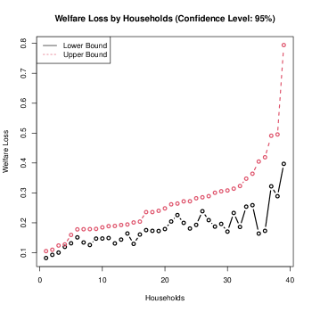
Figure 1: Household-Level Welfare Loss Bounds (Confidence Level $=0.95$)

We assume the prices are exogenous. To construct a $(1-\alpha)$ confidence set where $\alpha=0.05$, we first construct a $(1-\alpha/4)$ confidence set for each product by OLS. Specifically, we regress the inverse demand on price, and then construct a confidence interval for the inverse of the slope coefficient by the delta method. After intersecting this confidence interval with $[10^{-6},\infty)$ (assuming $\theta_{k}>0$, $k=1,2$), we do grid search with 5,000 grid nodes in this interval to obtain the intersection $CS^{\xi}_{k}(1-0.05/4)\cap CS^{LS}_{k}(1-0.05/4)$. Two out of 41 households have an empty confidence set.

For the welfare analysis for the 39 households with nonempty confidence sets, we compute the bounds in the same way as before. Figure 1 shows the lower and upper bounds on the welfare loss for the 39 households when both prices increase by 10%. The maximal welfare loss of the households are sorted in ascending order. Household heterogeneity is visible and the lower and upper bounds are relatively tight for most households.

6 Conclusion

In this paper, we propose a novel framework for individual-level welfare analysis. At any desired confidence level, our method can compute the bounds on the welfare loss under a price increase for every individual in a sample. The inferential method is computationally simple and scalable by solving a simple scalable optimization problem constrained by the confidence set for the parameters in the model. We also propose a new method to construct confidence sets under independence; the new method is easy to compute and robust to nonlinearity and weak instruments; it may be of independent interest.

Moving forward, it would be interesting to apply our framework to demand models such as Dubois, Griffith and Nevo (2014) and Allcott et al. (2019) to conduct individual-level welfare analysis.

Appendix A On the Shape and Size of the Confidence Set

In this appendix, we discuss how to learn the shape and size of our confidence set from two statistics: $\xi_{n}(P,Z)$ and $\xi_{n}(Y,Z)$. We first introduce the following lemma.

Lemma A.1.

Let $f$ be a strictly monotonic function. For two random variables $R^{(1)}$ and $R^{(2)}$, suppose we have an i.i.d. sample of them where there are no ties, then $\xi_{n}(f(R^{(1)}),R^{(2)})=\xi_{n}(R^{(1)},R^{(2)})$.

Proof.

Let $r_{i}^{0}$ and $r_{i}^{f}$ be the rankings of $R^{(2)}_{i}$ after the data are sorted by $R^{(1)}$ and $f(R^{(1)})$ in ascending order, respectively. If $f$ is strictly increasing, $r_{i}^{0}=r_{i}^{f}$ for all $i$; we are done. If $f$ is strictly decreasing, the order is reversed so $r_{i}^{f}=r_{n+1-i}^{0}$. Then by letting $n-i=j$,

$$\sum_{i=1}^{n-1}|r^{f}_{i+1}-r^{f}_{i}|= \sum_{i=1}^{n-1}|r^{0}_{n-i}-r^{0}_{n+1-i}|$$

$$= \sum_{j=n-1}^{1}|r^{0}_{j}-r^{0}_{j+1}|$$

$$= \sum_{i=1}^{n-1}|r^{0}_{i+1}-r^{0}_{i}|.$$

The desired result is obtained in view of equation (3.1). ∎

Remark A.1.

The conclusion in Lemma A.1 still holds when the $R^{(2)}_{i}$s have ties. It follows the same proof since the denominator in the formula of $\xi_{n}$ in footnote 1 is invariant to reordering.

Using our demand model with one product as an example, our inferential method focuses on the statistic $\xi_{n}(P-\theta/Y,Z)$ where $Z$ is a continuous instrument. Denote the true parameter by $\theta_{0}>0$. Our model says $P-\theta_{0}/Y=W$ so for an arbitrary $\theta$, $P-\theta/Y=(1-\theta/\theta_{0})P+(\theta/\theta_{0})W$. Then our $(1-\alpha)$ confidence set (3.3) is equal to

$$\left\{\theta\geq 0:\sqrt{n}\xi_{n}\left((1-\theta/\theta_{0})P+(\theta/\theta_{0})W,Z\right)\leq c_{1-\alpha}\right\}.$$

First, when $\theta=\theta_{0}$, the statistic becomes $\xi_{n}(W,Z)$. Under our independence assumption, $\sqrt{n}\xi_{n}(W,Z)\leq c_{1-\alpha}$ with probability approaching $(1-\alpha)$. Hence, our confidence set contains an interval around $\theta_{0}$ with probability approaching $(1-\alpha)$.

Now we proceed by verifying whether the confidence set contains regions near the boundaries of the parameter space $[0,\infty)$ (let the upper boundary be infinity).

When $\theta=0$, the statistic becomes $\xi_{n}(P,Z)$. If the instrument is relevant, i.e., $P\not\perp Z$, $\text{plim }\xi_{n}(P,Z)>0$ and thus $\sqrt{n}\xi_{n}(P,Z)\overset{p}{\to}\infty$. In finite samples, if $\sqrt{n}\xi_{n}(P,Z)>c_{1-\alpha}$, then there is an interval starting from 0 which is not contained in the confidence set.

When $\theta\to\infty$, let $f(x)=x/\theta$ which is strictly increasing in $x$ for any fixed $\theta>0$. Then by Lemma A.1, our statistic is equal to $\xi_{n}(P/\theta-(P-W)/\theta_{0},Z)$, which is in turn equal to $\xi_{n}(P/\theta-1/Y,Z)$ by the first order condition $P-W=\theta_{0}/Y$. By Theorem 1.1 in Chatterjee (2021), the probability limit of $\xi_{n}(P/\theta-1/Y,Z)$ and $\xi_{n}(-1/Y,Z)$ are $c\int\text{Var}(\mathbb{E}(1_{\{Z\geq t\}}|P/\theta-1/Y))d\mu(t)$ and $c\int\text{Var}(\mathbb{E}(1_{\{Z\geq t\}}|-1/Y))d\mu(t)$, respectively, where $c$ is some constant and $\mu$ is the law of $Z$. If $\int\text{Var}(\mathbb{E}(1_{\{Z\geq t\}}|P/\theta-1/Y))d\mu(t)$ is continuous in $\theta$, for sufficiently large $\theta$, $\xi_{n}(P/\theta-1/Y,Z)$ and $\xi_{n}(-1/Y,Z)$ are close with probability approaching 1 (w.p.a.1) by consistency. In the meantime, noting $Y>0$ and applying Lemma A.1 again, we have $\xi_{n}(-1/Y,Z)=\xi_{n}(Y,Z)$. As long as $Z\not\perp Y$, $\sqrt{n}\xi_{n}(Y,Z)>c_{1-\alpha}$ w.p.a.1. Therefore, there exists a $\bar{\theta}>\theta_{0}$ w.p.a.1 such that the confidence set does not contain $\theta>\bar{\theta}$, implying upper boundedness of the confidence set.

Figure 2 illustrates the shape of the function $\Xi_{n}(\theta)\coloneqq\sqrt{n}\xi_{n}(P-\theta/Y,Z)$ on $[0,\infty)$ following the analysis above. The four combinations $l_{1}$-$l_{3}$, $l_{1}$-$l_{4}$, $l_{2}$-$l_{3}$ and $l_{2}$-$l_{4}$ depict four graphs of the function depending on the magnitude of $\sqrt{n}\xi_{n}(P,Z)$ (the intersection point of the vertical axis and $l_{1}$ or $l_{2}$) and $\sqrt{n}\xi_{n}(Y,Z)$ (the asymptote of $l_{3}$ or $l_{4}$). The confidence set contains all $\theta$ at which the function is below the horizontal $c_{1-\alpha}$ line. Specifically, when $\sqrt{n}\xi_{n}(W,Z)<c_{1-\alpha}$, the four cases are as follows:

Case 1. $\sqrt{n}\xi_{n}(P,Z)>c_{1-\alpha}$ and $\sqrt{n}\xi_{n}(Y,Z)>c_{1-\alpha}$. Function $\Xi_{n}(\theta)$ is $l_{1}$-$l_{3}$. The confidence set is a bounded interval $[A,B]$.

Case 2. $\sqrt{n}\xi_{n}(P,Z)>c_{1-\alpha}$ and $\sqrt{n}\xi_{n}(Y,Z)\leq c_{1-\alpha}$. Function $\Xi_{n}(\theta)$ is $l_{1}$-$l_{4}$. The confidence set is $[A,\infty)$.

Case 3. $\sqrt{n}\xi_{n}(P,Z)\leq c_{1-\alpha}$ and $\sqrt{n}\xi_{n}(Y,Z)>c_{1-\alpha}$. Function $\Xi_{n}(\theta)$ is $l_{2}$-$l_{3}$. The confidence set is $[0,B]$.

Case 4. $\sqrt{n}\xi_{n}(P,Z)\leq c_{1-\alpha}$ and $\sqrt{n}\xi_{n}(Y,Z)\leq c_{1-\alpha}$. Function $\Xi_{n}(\theta)$ is $l_{2}$-$l_{4}$. The confidence set is the entire parameter space $[0,\infty)$.

To summarize, a large $\sqrt{n}\xi_{n}(P,Z)$ leads to a large lower bound for the confidence interval whereas a large $\sqrt{n}\xi_{n}(Y,Z)$ results in a small upper bound.

Figure 2: Function $\sqrt{n}\xi_{n}(P-\theta/Y,Z)$ and the Confidence Set

We can compute $\xi_{n}(P,Z)$ and $\xi_{n}(Y,Z)$ in our empirical applications. For instance, in the gasoline demand example, $\sqrt{n}\xi_{n}(P,Z)$ is quite large (59.74). Indeed, the lower bound of $CS^{\xi}$ in Table 3 is large; intersecting $CS^{\xi}$ with $CS^{LS}$ greatly improves the lower bound of the latter. For the upper bound, we compute $\sqrt{n}\xi_{n}(Y,Z)=-0.02$, smaller than the $0.95$th quantile of $N(0,0.4)$. Hence, $CS^{\xi}(0.95)$ is unbounded from above, so the intersecting approach improves its upper bound.

Appendix B Monotonicity, Concavity and Optimization

B.1 Monotonicity and Concavity of the Welfare Loss Function

In this section, we show that for any $c_{k}>0$, $k=1,\ldots,K$, function $\sum_{k=1}^{K}\theta_{k}\log(1+c_{k}/\theta_{k})$ is component-wise strictly increasing and strictly concave in $\bm{\theta}$ on $(0,\infty)^{K}$.

Monotonicity

For each $k$, there exists a $\zeta_{k}\in(0,c_{k}/\theta_{k})$ such that

$$\frac{d}{d\theta_{k}}\left[\theta_{k}\log(1+c_{k}/\theta_{k})\right]= \log\left(1+\frac{c_{k}}{\theta_{k}}\right)-\frac{c_{k}}{c_{k}+\theta_{k}}$$

$$= \frac{c_{k}}{\theta_{k}}\cdot\frac{1}{1+\zeta_{k}}-\frac{c_{k}}{c_{k}+\theta_{k}}$$

$$> \frac{c_{k}/\theta_{k}}{1+c_{k}/\theta_{k}}-\frac{c_{k}}{c_{k}+\theta_{k}}$$

$$= 0,$$

where the second equality is by the mean value theorem.

Concavity

For each $k$,

$$\frac{d^{2}}{d\theta_{k}^{2}}\left[\theta_{k}\log(1+c_{k}/\theta_{k})\right]=-\frac{c_{k}^{2}}{\theta_{k}(c_{k}+\theta_{k})^{2}}<0,\forall\theta_{k}>0.$$

Therefore, $\sum_{k=1}^{K}\theta_{k}\log(1+c_{k}/\theta_{k})$ is strictly concave on $(0,\infty)^{K}$.

B.2 Convex Optimization

Since the welfare loss function is concave in $\bm{\theta}$, we can maximize it by convex optimization algorithms when there are additional convex constraints. Many popular computer packages for convex optimization such as CVXR for R (Fu, Narasimhan and Boyd, 2020) and CVXPY for Python (Diamond and Boyd, 2016) use disciplined convex programming (DCP); DCP restricts the functions that can appear in the optimization problem and the way that the functions is composed. Specifically, such functions are called atomic functions and have known curvatures. Examples of such functions are $-\log(x)$ and $x^{2}$. The summands of our objective function (2.6) are not atomic functions. In this appendix, we introduce a technique to transform our problem to be DCP-solvable. It may be of independent interest.

The goal is to transform our objective function to be the sum of atomic functions kl_div, defined as $\text{kl\_div}(x_{1},x_{2})\coloneqq x_{1}\log(x_{1}/x_{2})-x_{1}+x_{2}$ for $x_{1}>0$ and $x_{2}>0$. To do so, we introduce an auxiliary variable $\bm{\gamma}\coloneqq(\gamma_{k})_{k}$ with an additional set of linear constraints $\tilde{\theta}_{k}-\gamma_{k}=-\Delta_{k}Y_{k}$ for all $k$. Since we only consider positive price change, $\gamma_{k}>0$ for all $k$. Then our objective function becomes

$$\sum_{k}\tilde{\theta}_{k}\log\left(1+\frac{\Delta_{k}Y_{k}}{\tilde{\theta}_{k}}\right)= -\sum_{k}\tilde{\theta}_{k}\log\left(\frac{\tilde{\theta}_{k}}{\tilde{\theta}_{k}+\Delta_{k}Y_{k}}\right)$$

$$= -\sum_{k}\left[\tilde{\theta}_{k}\log\left(\frac{\tilde{\theta}_{k}}{\tilde{\theta}_{k}+\Delta_{k}Y_{k}}\right)-\tilde{\theta}_{k}+(\tilde{\theta}_{k}+\Delta_{k}Y_{k})\right]+\sum_{k}\Delta_{k}Y_{k}$$

$$= -\sum_{k}\left[\tilde{\theta}_{k}\log\left(\frac{\tilde{\theta}_{k}}{\gamma_{k}}\right)-\tilde{\theta}_{k}+\gamma_{k}\right]+\sum_{k}\Delta_{k}Y_{k}$$

$$= -\sum_{k}\text{kl\_div}(\tilde{\theta}_{k},\gamma_{k})+\sum_{k}\Delta_{k}Y_{k}.$$

Since $\sum_{k}\Delta_{k}Y_{k}$ does not contain $(\bm{\tilde{\theta}},\bm{\gamma})$, we can solve the following minimization problem by DCP, obtain the minimizer, and compute the maximum of the original objective function:

$$\min_{\bm{\tilde{\theta}},\bm{\gamma}}\ \ \sum_{k}\text{kl\_div}(\tilde{\theta}_{k},\gamma_{k}),$$

$$s.t.\ \ \hat{L}_{k}(1-\alpha/K)\leq\tilde{\theta}_{k}\leq\hat{U}_{k}(1-\alpha/K),\ \forall k$$

$$\tilde{\theta}_{k}\geq 0,\ \forall k,$$

$$\tilde{\theta}_{k}-\gamma_{k}=-\Delta_{k}Y_{k},\ \forall k,$$

$$f_{j}(\tilde{\theta}_{1},\ldots,\tilde{\theta}_{K})\leq 0,\ j=1,\ldots,l,$$

$$g_{j}(\tilde{\theta}_{1},\ldots,\tilde{\theta}_{K})=0,\ j=1,\ldots,m,$$

where the convex functions $f_{1},\ldots,f_{l}$ and affine functions $g_{1},\ldots,g_{m}$ characterize additional constraints on the $\tilde{\theta}_{k}$s, for instance $\sum_{k=1}^{K}\tilde{\theta}_{k}=1$.

Appendix C Generalization of the Utility Function

One key step in our method is to express the welfare change as a known function of $(\bm{y}^{0},\bm{\theta},\bm{\Delta})$, by getting rid of the unobservable vector $\bm{W}$. In this section, we show that this is not driven by the choice of the log functions in the utility function (C). We derive a similar result under a general utility function.

Assume that a consumer with income level $I$ solves the following problem:

$$\max_{Y_{0},\bm{Y}} \ \ U(Y_{0},\bm{Y},\bm{W},\bm{\theta})\coloneqq Y_{0}+U_{0}(\bm{Y};\bm{\theta})+\bm{W}^{\prime}\bm{Y}$$

$$s.t. \ \ Y_{0}+\bm{P}^{\prime}\bm{Y}=I,$$

where $U_{0}(\cdot;\bm{\theta})$ is differentiable with the gradient denoted by $\nabla U_{0}(\cdot;\bm{\theta})$. We can solve for the optimal consumption $\bm{Y}^{*}$ as the solution to the following equation:

$$\nabla U_{0}(\bm{Y}^{*};\bm{\theta})=\bm{P}-\bm{W}.$$ (C.1)

Suppose at the true $\bm{\theta}$, function $\nabla U_{0}(\cdot;\bm{\theta})$ is one-to-one. Denoting its inverse by $D(\cdot;\bm{\theta})$, we then have

$$\bm{Y}^{*}(\bm{P},\bm{W};\bm{\theta})=D(\bm{P}-\bm{W};\bm{\theta}).$$ (C.2)

By $Y_{0}=I-\bm{P}^{\prime}\bm{Y}$ and suppressing the dependence of $\bm{Y}^{*}$ on $(\bm{P},\bm{W};\bm{\theta})$, we obtain the indirect utility as follows:

$$V(I,\bm{P},\bm{W},\bm{\theta})=I+U_{0}\left(\bm{Y}^{*};\bm{\theta}\right)-\left(\bm{P}-\bm{W}\right)^{\prime}\bm{Y}^{*}=I+U_{0}\left(\bm{Y}^{*};\bm{\theta}\right)-\nabla U_{0}(\bm{Y}^{*};\bm{\theta})^{\prime}\bm{Y}^{*},$$

where the second equality is by equation (C.1).

Now same as in Section 2, we consider the indirect utility function at price level $\bm{p}^{0}$ and $\bm{p}^{1}$ under $\bm{W}=\bar{\bm{w}}$. At $(\bm{p}^{1},\bar{\bm{w}})$, the counterfactual consumptions $\bm{y}^{1}\equiv\bm{Y}^{*}(\bm{p}^{1},\bar{\bm{w}};\bm{\theta})$ satisfy the following equation:

$$\bm{y}^{1}= D\left(\bm{p}^{1}-\bar{\bm{w}};\bm{\theta}\right)=D\left(\bm{p}^{0}-\bar{\bm{w}}+\bm{\Delta};\bm{\theta}\right)=D\left(\nabla U_{0}\left(\bm{y}^{0};\bm{\theta}\right)+\bm{\Delta};\bm{\theta}\right),$$

where the third equality is by $\bm{y}^{0}\equiv\bm{Y}^{*}(\bm{p}^{0},\bar{\bm{w}};\bm{\theta})$ and by equation (C.2). Therefore,

$$\text{WL}(\bm{\theta})$$

$$= V(I,\bm{p}^{0},\bar{\bm{w}},\bm{\theta})-V(I,\bm{p}^{1},\bar{\bm{w}},\bm{\theta})$$

$$= U_{0}\left(\bm{y}^{0};\bm{\theta}\right)-U_{0}\left(D\left(\nabla U_{0}\left(\bm{y}^{0};\bm{\theta}\right)+\bm{\Delta};\bm{\theta}\right);\bm{\theta}\right)$$

$$-\Big{[}\nabla U_{0}(\bm{y}^{0};\bm{\theta})^{\prime}\bm{y}^{0}-\nabla U_{0}(D\left(\nabla U_{0}\left(\bm{y}^{0};\bm{\theta}\right)+\bm{\Delta};\bm{\theta}\right);\bm{\theta})^{\prime}\cdot D\left(\nabla U_{0}\left(\bm{y}^{0};\bm{\theta}\right)+\bm{\Delta};\bm{\theta}\right)\Big{]}.$$

Although the expression is complicated, $U_{0}$, $\nabla U_{0}$ and $D$ are all known functions up to the unknown parameters $\bm{\theta}$. As $\bm{y}^{0}$ and $\bm{\Delta}$ are specified by the researcher, we can still optimize $\text{WL}(\bm{\theta})$ constrained by a confidence set of $\bm{\theta}$. In particular, one can verify that when $U_{0}(\bm{Y};\bm{\theta})=\sum_{k=1}^{K}\theta_{k}\log(Y_{k})$, the above expression for $\text{WL}(\bm{\theta})$ is equal to equation (2.6).

Remark C.1.

The function $\text{WL}(\bm{\theta})$ can still be optimized efficiently when it is concave. When that is no longer the case under the general $U_{0}$, one can optimize it by other nonconvex global optimization methods. Alternatively, if we assume $U_{0}(\bm{Y};\bm{\theta})=\sum_{k=1}^{K}U_{0,k}(Y_{k};\theta_{k})$ for some $U_{0,k}$s with known functional forms, then $\text{WL}(\bm{\theta})$ will become a sum of functions; each of these functions only depends on $(y^{0}_{k},\theta_{k},\Delta_{k})$ for one $k$; the specification adopted in the main text is one such example. Although these functions may not be globally concave, one may optimize each of them by grid search within the confidence set since there is only one unknown parameter. In this way, optimization can still be done efficiently and parallelly in $k$.

Appendix D Gasoline Demand: Smoothing the Instrument

In the gasoline demand example in Section 5.1, the instrumental variable only takes on 34 values ranging from 0.361 to 3.391. We treat this variable as continuous in the main text. In this appendix, we further smooth it by adding an independent $\text{Unif}[-0.1,0.1]$ noise term when applying the Chatterjee’s statistic. For 2SLS, we use the original instrument. The results are almost identical to those in Section 5.1; only the lower bound of the confidence interval using the intersection method and the corresponding lower bound on the welfare loss at the 0.9th quantile change to 1.436 and 0.803, respectively. The results are also robust to the magnitude of the uniform noise term.

References

- (1)
- Allcott et al. (2019) Allcott, Hunt, Rebecca Diamond, Jean-Pierre Dubé, Jessie Handbury, Ilya Rahkovsky, and Molly Schnell. 2019. “Food deserts and the causes of nutritional inequality.” Quarterly Journal of Economics, 134(4): 1793–1844.
- Bergsma and Dassios (2014) Bergsma, Wicher, and Angelos Dassios. 2014. “A Consistent Test of Independence Based on a Sign Covariance Related to Kendall’s tau.” Bernoulli, 20(2): 1006–1028.
- Blum, Kiefer and Rosenblatt (1961) Blum, JR, J Kiefer, and M Rosenblatt. 1961. “Distribution Free Tests of Independence Based on the Sample Distribution Function.” The Annals of Mathematical Statistics, 32(2): 485–498.
- Blundell, Horowitz and Parey (2017) Blundell, Richard, Joel Horowitz, and Matthias Parey. 2017. “Nonparametric estimation of a nonseparable demand function under the Slutsky inequality restriction.” Review of Economics and Statistics, 99(2): 291–304.
- Brown and Calsamiglia (2007) Brown, Donald J, and Caterina Calsamiglia. 2007. “The nonparametric approach to applied welfare analysis.” Economic Theory, 31(1): 183–188.
- Brown and Wegkamp (2002) Brown, Donald J, and Marten H Wegkamp. 2002. “Weighted minimum mean-square distance from independence estimation.” Econometrica, 70(5): 2035–2051.
- Brown, Deb and Wegkamp (2007) Brown, Donald J., Rahul Deb, and Marten H. Wegkamp. 2007. “Tests of independence in separable econometric models: Theory and application.” Cowles Foundation Discussion Paper 1395R2.
- Chatterjee (2021) Chatterjee, Sourav. 2021. “A New Coefficient of Correlation.” Journal of the American Statistical Association, 116(536): 2009–2022.
- Diamond and Boyd (2016) Diamond, Steven, and Stephen Boyd. 2016. “CVXPY: A Python-embedded modeling language for convex optimization.” Journal of Machine Learning Research, 17(83): 1–5.
- Dubé (2019) Dubé, Jean-Pierre. 2019. “Microeconometric models of consumer demand.” In Handbook of the Economics of Marketing. Vol. 1, 1–68. Elsevier.
- Dubois, Griffith and Nevo (2014) Dubois, Pierre, Rachel Griffith, and Aviv Nevo. 2014. “Do prices and attributes explain international differences in food purchases?” American Economic Review, 104(3): 832–867.
- Echenique, Lee and Shum (2011) Echenique, Federico, Sangmok Lee, and Matthew Shum. 2011. “The Money Pump as a Measure of Revealed Preference Violations.” Journal of Political Economy, 119(6): 1201–1223.
- Fu, Narasimhan and Boyd (2020) Fu, Anqi, Balasubramanian Narasimhan, and Stephen Boyd. 2020. “CVXR: An R Package for Disciplined Convex Optimization.” Journal of Statistical Software, 94(14): 1–34.
- Hoeffding (1948) Hoeffding, Wassily. 1948. “A Non-Parametric Test of Independence.” The Annals of Mathematical Statistics, 19(4): 546–557.
- Komunjer and Santos (2010) Komunjer, Ivana, and Andres Santos. 2010. “Semi-parametric estimation of non-separable models: a minimum distance from independence approach.” The Econometrics Journal, 13(3): S28–S55.
- Manski (1983) Manski, Charles F. 1983. “Closest empirical distribution estimation.” Econometrica, 51(2): 305–319.
- Nandy, Weihs and Drton (2016) Nandy, Preetam, Luca Weihs, and Mathias Drton. 2016. “Large-sample theory for the Bergsma-Dassios sign covariance.” Electronic Journal of Statistics, 10: 2287–2311.
- Poirier (2017) Poirier, Alexandre. 2017. “Efficient estimation in models with independence restrictions.” Journal of Econometrics, 196(1): 1–22.
- Shi, Drton and Han (2022) Shi, Hongjian, Mathias Drton, and Fang Han. 2022. “On the power of Chatterjee’s rank correlation.” Biometrika, 109(2): 317–333.
- Torgovitsky (2017) Torgovitsky, Alexander. 2017. “Minimum distance from independence estimation of nonseparable instrumental variables models.” Journal of Econometrics, 199(1): 35–48.
- Yanagimoto (1970) Yanagimoto, Takemi. 1970. “On measures of association and a related problem.” Annals of the Institute of Statistical Mathematics, 22(1): 57–63.