Torch-Choice: A PyTorch Package for Large-Scale Choice Modelling with Python

Abstract

The torch-choice is an open-source library for flexible, fast choice modeling with Python and PyTorch. torch-choice provides a ChoiceDataset data structure to manage databases flexibly and memory-efficiently. The paper demonstrates constructing a ChoiceDataset from databases of various formats and functionalities of ChoiceDataset. The package implements two widely used models, namely the multinomial logit and nested logit models, and supports regularization during model estimation. torch-choice incorporates the option to take advantage of GPUs for estimation, allowing it to scale to massive datasets while being computationally efficient. Models can be initialized using either R-style formula strings or Python dictionaries. We conclude with a comparison of the computational efficiencies of torch-choice and mlogit in R [1] as (1) the number of observations increases, (2) the number of covariates increases, and (3) the expansion of item sets. Finally, we demonstrate the scalability of torch-choice on large-scale datasets.

Keywords choice modelling  $\cdot$ Python  $\cdot$ PyTorch  $\cdot$ large scale dataset  $\cdot$ GPU acceleration

1 Introduction

Choice models are ubiquitous in economics, computer science, marketing, psychology, education and more fields. In consumer demand modeling, the researcher considers a setting where a consumer selects a product or brand from a set of alternatives, and the goal is to analyze how product characteristics affect consumer purchase decisions. These estimates can in turn be used to answer counterfactual questions about how purchases would change if, for example, prices or availability change. Choice models can be applied to aggregate market level demand data [2], cross-sectional individual choice data [3], and panel data where customer purchase events are tracked over time [4]. In transportation choice modeling, choice models are used to analyze intercity passenger travel mode choice [5, 6], and in spatial modeling to model location choice [7]. In labor economics, choice models are used to model labor supply and childcare decisions [8], and family labor supply [9]. In education, Item Response Theory (IRT) and related models are choice models [10, 11]. In psychology, choice models are used to model decision-making under uncertainty [12], and psychiatric treatment diagnoses [13]. In computer science, choice models are used to build recommendation systems [14] as well as for classification tasks such as spam filtering [15], image and character recognition [16], and many other applications.

Multinomial logistic regression and extensions are the most commonly used choice models. More recently, there has been work using choice models and their extensions (matrix-factorization, multilayer neural networks for choice modeling, Bayesian embeddings based choice models) to model restaurant choice [17], grocery shopping [18], inter-dependencies among choices when putting together a shopping basket [19], the welfare effects of recommendations [20], and to model labor market transitions [21]. For each of the models, either models based on multinomial logistic regression are used, or they are important baselines for further model development, creating a strong need for effective choice modeling software.

Recent years have seen the proliferation of various tools and software packages that go a long way in making it easy to estimate the parameters of choice models. While each of these have their particular strengths, there are important limitations of these packages when they are used with the goal of building flexible, fast choice models which scale to massive data.

In the discussion that follows, when we refer to R packages, we mean glm and mlogit. When we refer to Stata packages, we mean the entire suite of choice models offered in the packaged software. When we refer to flexible functional forms, we mean model specifications with user- and item-specific latent coefficients (latent variables). When we refer to regularization, we mean the ability to incorporate penalization or “shrinkage” of regression coefficients [22].

1. R packages allow the researcher to easily specify and learn models, and visualize the results, but they are not GPU-accelerated. Further, the estimation methods and data structures are not optimized for scalability (see Section 5). R also offers limited forms of latent variables in the specification of utility for multinomial and nested logit; specifically under random coefficients specifications, it does not allow for the retrieval of user-specific latent coefficients. R does not support regularization of model parameters.

2. Stata packages offer a similar user experience to R. They afford better computational efficiency by utilizing multiple CPU cores, although this is a paid feature, and can be prohibitively expensive for some users. However, these are still not GPU-accelerated features in Stata. Similar to R, while Stata supports user-specific latent coefficients in random coefficients models, the researcher must write additional code to access these coefficients, post estimation, while torch-choice provides these directly. Stata also does not support the regularization of model parameters.

3. Writing one’s own models in PyTorch has a steep learning curve for statisticians and econometricians, and setting up the training loop requires advanced programming expertise.

4. In python, the scikit-learn Logistic Regression [23] package is the go-to tool for computer scientists and allows for regularization, but it does not allow for specifying flexible functional forms, nor does it allow the availability of items to change across sessions. The pyBLP package [24] implements BLP-type random coefficients logit models in Python, and xlogit[25] implements choice models with a focus on the multinomial logit specification; torch-choice offers more flexible utility functional forms, leverages PyTorch and allows for using GPUs for faster estimation.

We propose torch-choice, a library for flexibly, fast choice modeling with PyTorch; it implements conditional and nested logit models, designed for both estimation and prediction. This package aims to address these limitations and fill the gap between tools used by econometricians/statisticians (R-style, end-to-end model training) and those computer scientists who are familiar with (PyTorch).

A limitation of torch-choice is that while it natively supports estimating user-specific coefficients in the setting of panel data, torch-choice estimates a constant coefficient (instead of distribution) for each user, and the same coefficient is applied across all sessions involving this user. It does not, however, learn the distribution over user-level parameters, and does not model that distribution. As such, it does not support random coefficients in cross-sectional data settings, where one can learn the parameters of distribution over user-level parameters in R, Stata, or xlogit in Python [25]. Please see section 4 for more details.

What are the advantages of using torch-choice?

1. It offers computational efficiency advantages because it is built on PyTorch, which allows for (optional) GPU acceleration. With PyTorch, our packages easily scale to large datasets of millions of choice records. In contrast, existing packages do not leverage GPUs, and use only one CPU core by default. Stata allows for the use of multiple cores, but this is a paid feature.

2. It uses a custom data structure that improves efficiency in memory and storage. The ChoiceDataset data structure avoids storing duplicate covariate information and offers an advantage in memory usage compared to traditional long and wide formats of choice datasets. Moreover, Pytorch allows for easy switching between different numeric precision (e.g., from float32 to float16); such a feature future reduces the memory requirement on large-scale datasets.

3. Model parameters are estimated using state-of-the-art first-order optimization algorithms such as Adam [26]; this makes it run in linear time (in the number of parameters) as compared to the quadratic, Hessian-based optimization routines used for optimizing choice models in R and Stata. Further, one can use any optimizer from the collection of state-of-the-art optimizers by in PyTorch, which have been tested by numerous modern machine learning practitioners. torch-choice supports second-order Quasi-Newton methods such as Limited-memory BFGS (LBFGS) for more precise optimization when computational resources permit[27].

4. torch-choice’s model estimation scheme is built upon PyTorch-Lightning[28], which facilitates rich model management such as learning rate decaying, early stopping, and parallel hyper-parameter tuning. These features are particularly useful when comparing multiple models over enormous datasets. Moreover, torch-choice complies TensorBoard logs during model estimation to illustrate the training progress, allowing for easy model diagnostics.

5. It natively reports user-level parameters if the functional form is so specified; while this can be accomplished using choice modeling software in R and Stata, it requires additional programming and expertise.

6. It allows the researcher to specify the functional form of utility (including specifying session-specific variables such as price), and to specify availability sets that may vary across sessions. This is not possible with scikit-learn and requires the researcher to write such functionality from scratch in standard PyTorch. Thus, torch-choice combines the benefits of scale obtained by using GPU acceleration with flexibility.

7. It supports nested logit; this is also not possible with scikit-learn and vanilla PyTorch.

8. It is open source, and can be easily customized and built upon. This is not so for choice models in Stata, though it is true for those in R and scikit-learn.

9. When using the multinomial logit with multiple categories, it allows sharing of parameters across categories [29], which is not supported in R, Stata, or Python.

The torch-choice library is publicly available on Github at: torch-choice github repository. Researchers can install our packages via pip following instructions at torch-choice on pip. We have prepared tutorials on the documentation website: torch-choice documentation website, where researchers can find the full documentation of APIs. Jupyter notebook [30] versions of these tutorials are available on Github at: torch-choice tutorial notebooks. Code demonstrated in this paper can be found in this Jupyter Notebook.

Section 2 outlines the choice problem torch-choice was built to model. Section 3 covers the data structures. Section 4 covers the models implemented in torch-choice. Section 5 shows performance benchmarks for torch-choice against another open source package, mlogit in R, and demonstrates its performance advantages. Finally, Section 6 concludes this paper.

2 The Choice Problem

We start by outlining the building blocks of the choice problem that will be processed with torch-choice. Models in torch-choice predict which item among all available items a user will choose given the context (where the context is referred to as a session). The paper refers to the basic unit of analysis as a choice record.

Definition 2.1 (Choice Records)

A choice record, also referred to as simply a record) is a triplet (user, item-chosen, session), where user is the identity of the user who made a choice, item chosen is the item the user chose, and an index for the session, where a session is characterized by contextual information such as the time-varying characteristics of the choice alternatives and the identities of available choice alternatives.

Figure 1 illustrates the layout of the ChoiceDataset data structure. Each row of the central dataframe in Figure 1 corresponds to a choice record.

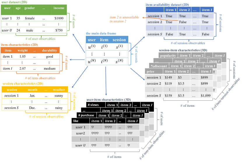
Figure 1: Illustration of ChoiceDataset Data Structure. The torch-choice supports user-session-item-specific observables as well, which is a 4D tensor. We are not drawing it in this illustration for succinctness.

Symbol	Definition
$N$	Number of choice records
$n$	Index of choice record, $n\in\{1,2,\dots,N\}$
$U,I,S,C$	Number of users/items/sessions/categories
$u^{(n)},i^{(n)},s^{(n)}$	User, item chosen, and session index of the $n^{th}$ choice record
$\mathcal{C}(i)$	Category of item $i$, $\mathcal{C}(i)\in\{1,2,\dots,C\}$
$I_{c}$	Items in category $c$, $I_{c}\subseteq\{1,2,\dots,I\}$
$I_{\mathcal{C}(i)}$	Items in the same category of item $i$
$\mathcal{D}$	The entire dataset $\{(u^{(n)},i^{(n)},s^{(n)})\}_{n=1}^{N}$
$\mathcal{D}^{(n)}$	The $n^{th}$ record in dataset $\mathcal{D}$, $(u^{(n)},i^{(n)},s^{(n)})$
$A$	The $S\times I$ binary matrices indicating the availability of items in each session
$A(s)$	The subset of items available in session $s$
$\mathcal{V}_{uis}$	The utility user $u$ gains from item $i$ in session $s$
$\mu_{uis}$	The deterministic part of utility $\mathcal{V}_{uis}=\mu_{uis}+\varepsilon_{uis}$
$\varepsilon_{uis}$	The stochastic part of utility $\mathcal{V}_{uis}=\mu_{uis}+\varepsilon_{uis}$
$P(i\mid u,s)$	The probability that user $u$ chooses item $i$ among items in $\mathcal{C}(i)$ in session $s$
$\hat{P}(i\mid u,s)$	The predicted probability that user $u$ chooses item $i$ among items in $\mathcal{C}(i)$ in session $s$

Table 1: Summary of Notations

2.1 Users, Items, and Sessions

Choice records are the fundamental unit of observation in choice modeling describing who (i.e., which user) chooses what (i.e., which item) under what context (i.e., in which session). Let $N$ denote the size of the dataset and $n\in\{1,2,\dots,N\}$ denote the index for records in the dataset. Let $\mathcal{D}$ denote the dataset and $\square^{(n)}$, the super-script with parentheses, denote the $n$-th record in the dataset, where $\square$ is a placeholder for the object of interest. Therefore, $\mathcal{D}^{(n)}=(u^{(n)},i^{(n)},s^{(n)})$ denotes the item chosen, the user involved, and the corresponding session index of the $n$-th record. Similarly, to represent subsets of a dataset, we can use superscripts. For instance, $\mathcal{D}^{(\text{train})}$ denotes the training set and $\mathcal{D}^{(\text{test})}$ denotes the test set.

The set of $U$ users is indexed by $u\in\{1,2,\dots,U\}$, while the set of $I$ items is indexed by $i\in\{1,2,\dots,I\}$. The set of sessions $S$ is indexed by $s\in\{1,2,\dots,S\}$. The set of items is partitioned into $C$ categories indexed by $c\in\{1,2,\dots,C\}$. Let $I_{c}$ denote the collection of items in category $c$, $I_{c}$’s are disjoint sets and $\bigcup_{c=1}^{C}I_{c}=\{1,2,\dots I\}$. Note that when we learn over multiple categories simultaneously, parameters that are not item-specific are the same across categories [29]. To learn per category parameters at the user and constant level, one needs to specify separate datasets and learn separate models over them. Let $\mathcal{C}(i)\in\{1,2,\dots,C\}$ denote the category of item $i$, $I_{\mathcal{C}(i)}$ represents items in the same category as item $i$.

The model assumes each user must choose exactly one item from each category (where one item may be defined to represent not selecting any items) and that choices are independent across categories and conditional on user preferences. The user $u$ chooses an item from each category to maximize their utility $\mathcal{V}_{uis}$ from item $i$ in the context of session $s$. We assume the utility can be decomposed into a deterministic utility $\mu_{uis}$ and an error term $\varepsilon_{uis}$ following the Gumbel distribution as in Equation (1).

$$\mathcal{V}_{uis}=\mu_{uis}+\varepsilon_{uis}$$ (1)

The same user will make choices from different categories in the same session, so that the dataset will contain multiple purchasing records with the same indices for user and session $(u,s)$ but different item indices $i$.

The utility $\mu_{uis}$ depends on the characteristics of users and items and other factors (e.g., the utility from iced coffee drops during winter time). We introduce the notion of session indexed by $s\in\{1,2,\dots,S\}$ to capture factors that vary by time and context.

The flexibility of sessions enables easier data management (e.g., observables and item availability) as we will see later.

2.2 Item Availability and Flexible Choice Sets

The session can be used to capture the fact that item availability may change over time. Our dataset admits a $S\times I$ binary matrix $A$ to indicate which items are available to be selected in each session. We use $A(s)$ to denote the set of available items in session $s$. All items are available all the time by default, i.e., $A(s)=\{1,2,\dots,I\}$ for all session $s$. Researchers should define the granularity of this matrix guided by the granularity with which item availability changes, along with the granularity of how users make decisions. For example, if the availability of items is the same in a day and a user faces at most one choice decision in a day, sessions may be defined at a day level; however, if users make more than one choice per day or if the availability of items is personalized to users, sessions will need to be more granular. Less granular session definitions encourage more efficient data management computationally. Note that in some applications, the prominence with which an item is displayed can also change over time; that can be captured as a time-varying item characteristic (i.e., an item-session observable).

2.3 Observable Tensors

The objective of our models is to predict utilities $\mu_{uis}$ as a function of user, item, and session characteristics called observable tensors.

$$\mu_{uis}=f_{\text{model}}(W_{u},X_{i},Z_{ui},T_{s},P_{is},M_{uis}).$$ (2)

The package supports all six types of observables with various dependencies on user $u$, item $i$, and session $s$. Observables are essentially high-dimensional arrays called tensors in machine learning literature. For example, an array $X$ of shape $U\times I\times 3$ can encapsulate three user-item-specific variables, indexing X[u,i,:] retrieves a vector in $\mathbb{R}^{3}$ for these observables corresponding to user u and item i. The following is a list of observable types supported and expected shapes of tensors/arrays encapsulating them.

1. User observable tensors $\in\mathbb{R}^{U\times K_{\text{user}}}$ vary only with the user identity, for example, time-invariant user demographics.

2. Item observable tensors $\in\mathbb{R}^{I\times K_{\text{item}}}$ vary only with the item index, for example, the length of a movie.

3. Session observable tensors $\in\mathbb{R}^{S\times K_{\text{session}}}$ vary only with the session identifier. For example, if the session is defined as the date, the daily weather could be a session observable.

4. User-item observable tensors $\in\mathbb{R}^{U\times I\times K_{\text{user-item}}}$ depend on both user and item. For example, a user-item session observable can capture users’ ratings of different items, assuming users cannot change their ratings. User-item observable tensors can also capture interaction effects between users and items.

5. Item-session observable tensors $\in\mathbb{R}^{S\times I\times K_{\text{item-session}}}$ are session-and-item-specific observables that vary with both session and item, for example, prices of items if sessions are defined as dates.

6. User-session-item observable tensors $\in\mathbb{R}^{U\times S\times I\times K_{\text{user-session-item}}}$ are specific to the combination of user, item, and session. For example, a user-session-item observable can store the number of times a user purchased an item prior to a specific date.

Performance note The user-session-item observable tensor can be extremely large and cause out-of-memory issues even at moderate levels of $U$, $I$, and $S$. For example, suppose we are modeling shopping data with customers as users and dates as sessions; there is a user-session-item-specific observable $x_{uis}$. Storing the complete $x_{uis}$ requires $U\times S\times I$ entries. Often, each customer only shops on a couple of dates, say three dates on average and $S\gg 3$. We can redefine sessions to be all existing pairs of (customer, date), and $X$ becomes a session-item-specific observable instead. Storing $X$ as a session-item-observable only requires $3\times S\times I$ entries, a factor of $U/3$ reduction.

Since torch-choice leverages PyTorch and GPU accelerations, all observables need to be numerical, and indices of users/items/sessions should be consecutive integers. Raw item names can be encoded easily with sklearn.preprocessing.LabelEncoder or OrdinalEncoder.

user_index	session_index	item_index
Amy	Sep-17-2021-Store-A	banana
Ben	Sep-17-2021-Store-B	apple
Ben	Sep-16-2021-Store-A	orange
Charlie	Sep-16-2021-Store-B	apple
Charlie	Sep-16-2021-Store-B	orange

Table 2: The Example Dataset

2.4 Model Prediction

We assume each user selects at most one item from each item category each session by maximizing his/her utility $\mathcal{V}_{uis}$ within each category. When users are choosing over items, we can write utility $\mathcal{V}_{uis}$ that user $u$ derives from item $i$ in session $s$ as:

$$\mathcal{V}_{uis}=\mu_{uis}+\varepsilon_{uis}$$ (3)

where $\varepsilon$ is an unobserved random error term. If we assume i.i.d. extreme value type I errors for $\varepsilon_{uis}$, which leads to the logistic probabilities of user $u$ choosing item $i$ among $I_{C(i)}$ (i.e., items in the same category as $i$) in session $s$, as shown by McFadden[31], and as often studied in Econometrics.

Given the distributional assumption on $\varepsilon_{uis}$, the probability that user $u$ chooses item $i$ in session $s$ is captured by the logistic function

$$P(i\mid us)=\frac{\exp\left(\mu_{uis}\right)}{\sum_{\ell\in A(s)\cap I_{C(i)}}\exp\left(\mu_{u\ell s}\right)}$$ (4)

where $A(s)$ is the set of items available in session $s$ (i.e., the choice set), and $I_{C(i)}$ is the set of items in the same category as item $i$. The probability in Equation (4) is normalized over available items only; therefore, probabilities of choosing unavailable item items are zero. The mean utility $\mu_{uis}$ for a user, item, and session is specified according to a functional form, and we consider different combinations of observable and latent variables, each of which corresponds to a distinct version of the model.

Equation (5) describes the general form of the utility function in conditional logit models. Greek letters with tilde and prime (e.g., $\alpha,\tilde{\alpha}_{i},\alpha_{u}^{\prime}$) are coefficients to be estimated; capital letters denote observables; subscripts of them denote their dependencies on user $u$, item $i$, and session $s$.

$$\begin{split}\mu_{uis}&=\underbrace{\alpha+\tilde{\alpha}_{i}+\alpha_{u}^{\prime}}_{\text{fixed effects}}+\underbrace{\beta W_{u}^{\text{I}}+\tilde{\beta}_{i}W_{u}^{\text{II}}+\beta_{u}^{\prime}W_{u}^{\text{III}}}_{\text{user observables}}+\underbrace{\gamma X_{i}^{\text{I}}+\tilde{\gamma}_{i}X_{i}^{\text{II}}+\gamma_{u}^{\prime}X_{i}^{\text{III}}}_{\text{item observables}}+\underbrace{\eta Z_{ui}^{\text{I}}+\tilde{\eta}_{i}Z_{ui}^{\text{II}}+\eta_{u}^{\prime}Z_{ui}^{\text{III}}}_{\text{user-item observables}}\\ &+\underbrace{\tau T_{s}^{\text{I}}+\tilde{\tau}_{i}T_{s}^{\text{II}}+\tau_{u}^{\prime}T_{s}^{\text{III}}}_{\text{session observables}}+\underbrace{\delta P_{is}^{\text{I}}+\tilde{\delta}_{i}P_{is}^{\text{II}}+\delta_{u}^{\prime}P_{is}^{\text{III}}}_{\text{item-session observables}}+\underbrace{\omega M_{uis}^{\text{I}}+\tilde{\omega}_{i}M_{uis}^{\text{II}}+\omega^{\prime}_{i}M_{uis}^{\text{III}}}_{\text{user-session-item observables}}\end{split}$$ (5)

For example, the specification in Equation (6) allows for user observables ($W_{u}$), item observables ($X_{i}$), and item-session observable ($P_{is}$), and intercepts that vary with the item:

$$\mu_{uis}=\alpha_{i}+\beta_{u}X_{i}+\gamma W_{u}+\delta_{i}P_{is}$$ (6)

The Greek letters $\alpha_{i}$, $\beta_{u}$, $\gamma$, and $\delta_{i}$ denote coefficients to be estimated. These coefficients can be interpreted as the individual user fixed effect, impacts of item characteristics, user characteristics, and (session, item)-specific characteristics on the mean utility for user $u$ for item $i$. Researchers can add user-item observable interactions by constructing the corresponding item-session specific observable. The torch-choice package offers flexible ways to estimate the mean utility $\mu_{uis}$ beyond this example; the model section will cover these aspects in detail.

Beyond the basic and widely implemented multinomial logit model, the torch-choice library provides two widely used classes of choice models, the conditional logit model (CLM) and the nested logit model (NLM) to model $\mu_{uis}$. The standard multinomial logit model is nested in the conditional logit model, and so is treated as a special case. The nested logit model relaxes the i.i.d. assumption on $\varepsilon_{uis}$.

In each of the conditional logit and nested logit models, researchers can specify the functional form they want to use for observables. Each model takes user and session information $(u^{(n)},s^{(n)})$ together with observables and outputs the predicted probability of purchasing each $\ell\in\{1,2,\dots,I\}$, denoted as $\hat{P}(\ell\mid u^{(n)},s^{(n)})$. In cases when not all items are available, the model sets the probability of unavailable items to zero and normalizes probabilities among available items. By default, model coefficients are estimated using the gradient descent algorithm to maximize log-likelihood in Equation (7). Since torch-choice is built upon PyTorch, any other optimization algorithms supported by PyTorch can be used as well. Please refer to our online documentation for details regarding applying alternative optimization algorithms.

$$\text{log-likelihood}=\sum_{n=1}^{N}\log\hat{P}(i^{(n)}\mid u^{(n)},s^{(n)})$$ (7)

The models implemented in torch-choice offer flexible ways to estimate the deterministic part $\mu_{uis}$. Given the Gumbel distribution of $\varepsilon_{uis}$ and the independence of irrelevant items assumption, the predicted probability for choosing item $i$ among all items in the same category $I_{\mathcal{C}(i)}$ is a function of utilities $\{\mu_{ui^{\prime}s}\}_{i^{\prime}\in I_{\mathcal{C}(i)}}$ from the model. The exact functional form differs by model, and we defer the discussion to the model section. The form of predicted probabilities for any given specificaton of $\mu$ is a normalized exponential function (“softmax”) function in Equation (8).

$$P(i|u,s)=\begin{cases}\frac{\exp\left(\mu_{uis}\right)}{\sum_{i^{\prime}\in I_{\mathcal{C}(i)}\cap A(s)}\exp\left(\mu_{ui^{\prime}s}\right)}&\text{if $i\in A(s)$, i.e., $i$ is available in session $s$.}\\ 0&\text{otherwise}\end{cases}$$ (8)

3 Data Structures

This section covers the ChoiceDataset class in the torch-choice library. ChoiceDataset is a specialized instantiation of PyTorch’s Dataset class. It inherits support for all of the functionality of PyTorch’s Dataset class, including subsetting, indexing, and random sampling. Most importantly, GPU memory is often much more scarce on modern machines, ChoiceDataset is manage information in a memory-efficient manner. Existing packages such as xlogit in Python [25] and mlogit [1] in R require the data to be in a long-format or wide-format, which store duplicate information. ChoiceDataset minimizes its memory footage via its specialized structure eliminating redundant information. Moreover, all information in ChoiceDataset is stored as PyTorch tensors, which allows researchers to leverage half-precision floats to further improve memory efficiency and seamless data transfer between CPU and GPU.

3.1 Constructing a Choice Dataset, Method 1: Easy Data Wrapper Class

The torch-choice provides two methods to build ChoiceDataset; the first method is to use the EasyDataWrapper class, which is a wrapper class that converts pandas DataFrame in long-format to ChoiceDataset.

The EasyDataWrapper only requires that the researcher (1) load dataframes to Python (for example, using pandas tools to load various types of data files including CSV, TSV, Stata database, and Excel spreadsheet) and (2) usage of pandas to pre-process the dataset.

We load the car-choice dataset to demonstrate torch-choioce’s data wrapper utility. The car-choice dataset is a synthetic dataset on consumers’ choices regarding the nationality of cars; the dataset was modified from Stata’s tutorial dataset.

⬇

1car_choice = pd.read_csv("https://raw.githubusercontent.com/gsbDBI/torch-choice/main/tutorials/public_datasets/car_choice.csv")

The dataset is in “long” format: multiple rows constitute a single choice record.

Table 3 presents the first 30 rows of the car-choice dataset, in which each user (consumer) only made one choice. The first four rows with record_id == 1 correspond to the first purchasing record. It means that consumer 1 was deciding on four types of cars (i.e., items) and chose American car (since the purchase == 1 in that row of American car). Not all cars were available all the time. For example, there is no row in the dataset with session_id == 4 & car == "Korean", which means only American, Japanese, and European cars were available in the fourth session.

Table 3: The first 30 rows of the car-choice dataset.

record_id	session_id	consumer_id	car	purchase	gender	income	speed	discount	price
1	1	1	American	1	1	46.699997	10	0.94	90
1	1	1	Japanese	0	1	46.699997	8	0.94	110
1	1	1	European	0	1	46.699997	7	0.94	50
1	1	1	Korean	0	1	46.699997	8	0.94	10
2	2	2	American	1	1	26.100000	10	0.95	100
2	2	2	Japanese	0	1	26.100000	8	0.95	70
2	2	2	European	0	1	26.100000	7	0.95	20
2	2	2	Korean	0	1	26.100000	8	0.95	10
3	3	3	American	0	1	32.700000	10	0.90	80
3	3	3	Japanese	1	1	32.700000	8	0.90	60
3	3	3	European	0	1	32.700000	7	0.90	20
4	4	4	American	1	0	49.199997	10	0.81	50
4	4	4	Japanese	0	0	49.199997	8	0.81	40
4	4	4	European	0	0	49.199997	7	0.81	30
5	5	5	American	0	1	24.300000	10	0.87	80
5	5	5	Japanese	0	1	24.300000	8	0.87	30
5	5	5	European	1	1	24.300000	7	0.87	30
6	6	6	American	1	0	39.000000	10	0.83	100
6	6	6	Japanese	0	0	39.000000	8	0.83	60
6	6	6	European	0	0	39.000000	7	0.83	10
7	7	7	American	0	1	33.000000	10	0.98	100
7	7	7	Japanese	0	1	33.000000	8	0.98	60
7	7	7	European	1	1	33.000000	7	0.98	40
7	7	7	Korean	0	1	33.000000	8	0.98	10
8	8	8	American	1	1	20.300000	10	0.88	60
8	8	8	Japanese	0	1	20.300000	8	0.88	50
8	8	8	European	0	1	20.300000	7	0.88	30
9	9	9	American	0	1	38.000000	10	0.93	90
9	9	9	Japanese	1	1	38.000000	8	0.93	90
9	9	9	European	0	1	38.000000	7	0.93	20

The EasyDataWrapper requires a long-format main dataset with the following columns:

1. purchase_record_column: a column identifies record (also called case in Stata syntax). In this tutorial, the record_id column is the identifier. For example, the first 4 rows of the dataset (see above) has record_id == 1, which implies that the first 4 rows together constitute the first record.

2. item_name_column: a column identifies names of items, which is car in the dataset above. This column provides information above the availability as well. As mentioned above, there is no column with car == "Korean" in the fourth session (session_id == 4), indicating that the Korean car was not available in that session.

3. choice_column: a column with values $\in\{0,1\}$ identifies the choice made by the consumer in each record, which is the purchase column in the car choice dataset. There should be exactly one row per record (i.e., rows with the same values in purchase_record_column) with value one, while the values are zeros for all other rows.

4. user_index_column: an optional column identifies the user making the choice, which is consumer_id in the car-choice dataset.

5. session_index_column: an optional column identifies the session of choice, which is session_id in the above dataframe.

3.1.1 Adding Observables

The next step is to identify observables to be incorporated in the model. In the car-choice dataset, we want to add (1) gender and income columns as user-specific observables; (2) speed as item-specific observable; (3) discount as session-specific observable; (4) price as (session, item)-specific observable.

3.1.2 Adding Observables, Method 1: Observables Derived from Columns of the Main Dataset

The above car-choice dataframe already includes observables we want to add. The first approach to adding observables is to simply identify these columns while initializing the EasyDatasetWrapper object. This is accomplished by supplying a list of column names to each of {user, item, session, itemsession}_observable_columns keyword arguments. For example, we assign

⬇

1user_observable_columns=["gender", "income"]

to specify user-specific observables from the gender and income columns of the main dataframe. The code snippet below shows how to initialize the EasyDatasetWrapper object.

⬇

1from torch_choice.utils.easy_data_wrapper import EasyDatasetWrapper

2data_wrapper_from_columns = EasyDatasetWrapper(

3 main_data=car_choice,

4 purchase_record_column=’record_id’,

5 choice_column=’purchase’,

6 item_name_column=’car’,

7 user_index_column=’consumer_id’,

8 session_index_column=’session_id’,

9 user_observable_columns=[’gender’, ’income’],

10 item_observable_columns=[’speed’],

11 session_observable_columns=[’discount’],

12 itemsession_observable_columns=[’price’])

13

14data_wrapper_from_columns.summary()

15dataset = data_wrapper_from_columns.choice_dataset

16# ChoiceDataset(label=[], item_index=[885], provided_num_items=[], user_index=[885], session_index=[885], item_availability=[885, 4], item_speed=[4, 1], user_gender=[885, 1], user_income=[885, 1], session_discount=[885, 1], itemsession_price=[885, 4, 1], device=cpu)

The data_wrapper.summary() method can be used to print out a summary of the dataset. The ChoiceDataset object can be accessed by the wrapper using data_wrapper.choice_dataset.

3.1.3 Adding Observables, Method 2: Added as Separated DataFrames

Researchers can also construct dataframes and use dataframes to supply different observables. This is useful in the case of longitudinal data or when users choose items from multiple categories, so that there are multiple choice records by the same user. Suppose there are $K$ choice records for each of the $U$ users. Using a single dataframe for all variables requires a lot of memory and repeated data, while using a separate dataframe mapping user index to user observables only requires $U$ entries for each observable. Similarly, storing item information or item-session information in long-format data leads to inefficient storage.

Dataframes for user-specific observables need to contain a column of user IDs (e.g., consumer_id), this column should have exactly the same name as the column containing user indices. Similarly, for item-specific observables, the dataframe should contain a column of item names (i.e., car in this car-choice example); session identifier column session_id needs to be present for session-specific observable dataframes, and both item and session identifiers need to be present for item-session-specific observable dataframes.

The following code snippet extracts dataframes for observables from the car-choice dataframe.

⬇

1# create dataframes for gender and income. The dataframe for user-specific observable needs to have the ‘consumer_id‘ column.

2gender = car_choice.groupby(’consumer_id’)[’gender’].first().reset_index()

3income = car_choice.groupby(’consumer_id’)[’income’].first().reset_index()

4# alternatively, put gender and income in the same dataframe.

5gender_and_income = car_choice.groupby(’consumer_id’)[[’gender’, ’income’]].first().reset_index()

6# speed as item observable, the dataframe requires a ‘car‘ column.

7speed = car_choice.groupby(’car’)[’speed’].first().reset_index()

8# discount as session observable. the dataframe requires a ‘session_id‘ column.

9discount = car_choice.groupby(’session_id’)[’discount’].first().reset_index()

10# create the price as itemsession observable, the dataframe requires both ‘car‘ and ‘session_id‘ columns.

11price = car_choice[[’car’, ’session_id’, ’price’]]

12# fill in NANs for (session, item) pairs that the item was not available in that session.

13price = price.pivot(’car’, ’session_id’, ’price’).melt(ignore_index=False).reset_index()

Then, researchers can initialize the EasyDatasetWrapper object with these dataframes via {user, item, session, itemsession}_observable_data keyword arguments.

⬇

1data_wrapper_from_dataframes = EasyDatasetWrapper(

2 main_data=car_choice,

3 purchase_record_column=’record_id’,

4 choice_column=’purchase’,

5 item_name_column=’car’,

6 user_index_column=’consumer_id’,

7 session_index_column=’session_id’,

8 user_observable_data={’gender’: gender, ’income’: income},

9 # alternatively, supply gender and income as a single dataframe.

10 # user_observable_data={’gender_and_income’: gender_and_income},

11 item_observable_data={’speed’: speed},

12 session_observable_data={’discount’: discount},

13 itemsession_observable_data={’price’: price})

14

15# the second method creates exactly the same ChoiceDataset as the previous method.

16assert data_wrapper_from_dataframes.choice_dataset == data_wrapper_from_columns.choice_dataset

The EasyDataWrapper also support the mixture of above methods: in the following example, we supply user, item, and session-specific observables (i.e., gender, income, speed, and discount) as dataframes but the item-session specific observable (i.e., price) using the corresponding column name.

⬇

1data_wrapper_mixed = EasyDatasetWrapper(

2 main_data=car_choice,

3 purchase_record_column=’record_id’,

4 choice_column=’purchase’,

5 item_name_column=’car’,

6 user_index_column=’consumer_id’,

7 session_index_column=’session_id’,

8 user_observable_data={’gender’: gender, ’income’: income},

9 item_observable_data={’speed’: speed},

10 session_observable_data={’discount’: discount},

11 itemsession_observable_columns=[’price’])

12

13# these methods create exactly the same choice dataset.

14assert data_wrapper_mixed.choice_dataset == data_wrapper_from_columns.choice_dataset == data_wrapper_from_dataframes.choice_dataset

3.2 Constructing a Choice Dataset, Method 2: Building from Tensors

As discussed above, storing data in a long format is not memory efficient due to repeated data. torch-choice enables storage of observables as separate tensors.

This section demonstrates an example of creating a dataset from observable and index tensors. We use a randomly generated dataset with $N=10,000$ records from $U=10$ users, $I=4$ items and $S=500$ sessions. We generate random observable tensors for user, item, session, and item-session observables from independent multivariate Gaussian distributions following Equation (9). For simplicity, we generate data where all items are available in all sessions.

$$\begin{aligned} W_{u}&\sim\mathcal{N}(\bm{0},I_{128\times 128})\quad\forall u\in\{1,2,\dots,U\}\\ X_{i}&\sim\mathcal{N}(\bm{0},I_{64\times 64})\quad\forall i\in\{1,2,\dots,I\}\\ Z_{ui}&\sim\mathcal{N}(\bm{0},I_{32\times 32})\quad\forall(u,i)\in\{1,2,\dots,U\}\times\{1,2,\dots,I\}\\ T_{s}&\sim\mathcal{N}(\bm{0},I_{10\times 10})\quad\forall s\in\{1,2,\dots,S\}\\ P_{is}&\sim\mathcal{N}(\bm{0},I_{12\times 12})\quad\forall(i,s)\in\{1,2,\dots,I\}\times\{1,2,\dots,S\}\\ M_{uis}&\sim\mathcal{N}(\bm{0},I_{8\times 8})\quad\forall(u,i,s)\in\{1,2,\dots,U\}\times\{1,2,\dots,I\}\times\{1,2,\dots,S\}\\ u^{(n)}&\sim\text{Unif}(\{1,2,\dots,U\})\quad\forall n\in\{1,2,\dots,N\}\\ i^{(n)}&\sim\text{Unif}(\{1,2,\dots,I\})\quad\forall n\in\{1,2,\dots,N\}\\ s^{(n)}&\sim\text{Unif}(\{1,2,\dots,S\})\quad\forall n\in\{1,2,\dots,N\}\end{aligned}$$ (9)

The code snippet below builds a ChoiceDataset object from randomly generated $(u^{(n)},i^{(n)},s^{(n)})$ and observable tensors. This construction assumes that all items are available in all sessions, since the item_availability argument is not specified.

⬇

1N = 10000

2numusers = 10

3num_items = 4

4num_sessions = 500

5

6

7user_obs = torch.randn(num_users, 128)

8item_obs = torch.randn(num_items, 64)

9useritem_obs = torch.randn(num_users, num_items, 32)

10session_obs = torch.randn(num_sessions, 10)

11itemsession_obs = torch.randn(num_sessions, num_items, 12)

12usersessionitem_obs = torch.randn(num_users, num_sessions, num_items, 8)

13

14item_index = torch.LongTensor(np.random.choice(num_items, size=N))

15user_index = torch.LongTensor(np.random.choice(num_users, size=N))

16session_index = torch.LongTensor(np.random.choice(num_sessions, size=N))

17item_availability = torch.ones(num_sessions, num_items).bool()

18

19dataset = ChoiceDataset(

20 item_index=item_index,

21 user_index=user_index, session_index=session_index, item_availability=item_availability,

22 # observable tensors are supplied as keyword arguments with special prefixes.

23 user_obs=user_obs, item_obs=item_obs, useritem_obs=useritem_obs, session_obs=session_obs, itemsession_obs=itemsession_obs, usersessionitem_obs=usersessionitem_obs)}

The ChoiceDataset is expecting the following arguments at its initialization.

1. item_index captures item chosen in each record $(i^{(n)})_{n=1}^{N}$.

2. user_index captures the user making decision in each record $(u^{(n)})_{n=1}^{N}$. user_index is optional. By default, the same user is making decisions repeatedly.

3. session_index captures the corresponding session of each record $(s^{(n)})_{n=1}^{N}$. session_index is optional. By default, each record has its own session.

4. item_availability is the binary availability matrix $A$ with shape $S\times I$. item_availability is optional. By default, all items are available in all sessions.

observable type	tensor shape	keyword argument prefix requirement
item-specific	($I$, number of observables)	item_<obs_name>
user-specific	($U$, number of observables)	user_<obs_name>
(user, item)-specific	($U$, $I$, number of observables)	useritem_<obs_name>
session-specific	($S$, number of observables)	session_<obs_name>
(item, session)-specific	($S$, $I$, number of observables)	itemsession_<obs_name>
(user, session, item)-specific	($U$, $S$, $I$, number of observables)	usersessionitem_<obs_name>

Table 4: Expected Shapes of Observable Tensors. Dimensions of tensors are always ordered as user dimension first, then session dimension, and then item dimension.

As mentioned previously, all observable tensors should meet shape requirements in Table 4.

Further, the data structure in torch-choice package utilizes variable name prefixes to keep track of observables’ variation. Observable tensors need to follow naming conventions for ChoiceDataset to build correctly. While constructing the ChoiceDataset with observable tensor keyword arguments, observable tensors are named with prefixes indicating how they depend on the user (with user_ prefix), item (with item_ prefix), session (with session_ prefix), and both of (item, session) (with itemsession_ prefix) .

For example, suppose we have a tensor X for user income of shape $(U,1)$. The income observable should be introduced as ChoiceDataset(..., user_income=X, ...), initializing the dataset with ChoiceDataset(..., income_of_user=X, ...) will introduce errors. Table 4 summarizes the naming requirement for different types of observable tensors.

When multiple observable tensors of the same level of variation are needed, researchers can include as many keyword arguments as needed, as long as they follow the prefix requirement. For example, ChoiceDataset(..., user_income=X, user_age=Z, user_education=E...) includes three different user-specific observable tensors. Such a feature is particularly useful when you want, for example, an item-specific effect on users’ income but a constant effect on users’ education levels.

3.3 Functionalities of the Choice Dataset

This section overviews the functionalities of the ChoiceDataset class. The command print(dataset) provides a quick overview of shapes of tensors included in the object as well as where the dataset is located (i.e., in CPU memory or GPU memory). The dataset.summary() method offers more detailed information about the dataset.

⬇

1print(dataset)

2# ChoiceDataset(label=[], item_index=[10000], user_index=[10000], session_index=[10000], item_availability=[500, 4], user_obs=[10, 128], item_obs=[4, 64], session_obs=[500, 10], price_obs=[500, 4, 12], device=cpu)

The dataset.num_{users, items, sessions} attribute can be used to obtain the number of users, items, and sessions, which are determined automatically from the {user, item, session}_obs tensors provided while initializing the dataset object. The len(dataset) reveals the number of records $N$ in the dataset.

⬇

1print(f’{dataset.num_users=:}’)

2# dataset.num_users=10

3print(f’{dataset.num_items=:}’)

4# dataset.num_items=4

5print(f’{dataset.num_sessions=:}’)

6# dataset.num_sessions=500

7print(f’{len(dataset)=:}’)

8# len(dataset)=10000

The ChoiceDataset offers a clone method to make a copy of the dataset; researchers can modify cloned dataset safely without changing the original dataset.

⬇

1# clone

2print(dataset.item_index[:10])

3# tensor([2, 2, 3, 1, 3, 2, 2, 1, 0, 1])

4dataset_cloned = dataset.clone()

5# modify the cloned dataset.

6dataset_cloned.item_index = 99 * torch.ones(num_sessions)

7print(dataset_cloned.item_index[:10])

8# the cloned dataset is changed.

9# tensor([99., 99., 99., 99., 99., 99., 99., 99., 99., 99.])

10print(dataset.item_index[:10])

11# the original dataset does not change.

12# tensor([2, 2, 3, 1, 3, 2, 2, 1, 0, 1])

ChoiceDataset objects can be moved between host memory (i.e., CPU memory) and device memory (i.e., GPU memory) using the dataset.to() method. The dataset.to() method moves all tensors in the ChoiceDataset to the target device. The following code runs only on a machine with a compatible GPU as well as a GPU-compatible version of PyTorch installed. The dataset._check_device_consistency() method checks if all tensors are on the same device. For example, an attempt to move the item_index tensor to CPU without moving other tensors will result in an error message.

⬇

1# move to device

2print(f’{dataset.device=:}’)

3# dataset.device=cpu

4print(f’{dataset.device=:}’)

5# dataset.device=cpu

6print(f’{dataset.user_index.device=:}’)

7# dataset.user_index.device=cpu

8print(f’{dataset.session_index.device=:}’)

9# dataset.session_index.device=cpu

10

11dataset = dataset.to(’cuda’)

12

13print(f’{dataset.device=:}’)

14# dataset.device=cuda:0

15print(f’{dataset.item_index.device=:}’)

16# dataset.item_index.device=cuda:0

17print(f’{dataset.user_index.device=:}’)

18# dataset.user_index.device=cuda:0

19print(f’{dataset.session_index.device=:}’)

20# dataset.session_index.device=cuda:0

⬇

1dataset.checkdevice_consistency()

⬇

1# NOTE: this cell will result errors, this is intentional.

2dataset.item_index = dataset.item_index.to(’cpu’)

3dataset.checkdevice_consistency()

4# ---------------------------------------------------------------------------

5

6# Exception Traceback (most recent call last)

7

8# <ipython-input-56-40d626c6d436> in <module>

9 # 1 # # NOTE: this cell will result errors, this is intentional.

10 # 2 dataset.item_index = dataset.item_index.to(’cpu’)

11# ----> 3 dataset._check_device_consistency()

12

13

14# ~/Development/torch-choice/torch_choice/data/choice_dataset.py in _check_device_consistency(self)

15 # 180 devices.append(val.device)

16 # 181 if len(set(devices)) > 1:

17# --> 182 raise Exception(f’Found tensors on different devices: {set(devices)}.’,

18 # 183 ’Use dataset.to() method to align devices.’)

19 # 184

20

21

22# Exception: ("Found tensors on different devices: {device(type=’cuda’, index=0), device(type=’cpu’)}.", ’Use dataset.to() method to align devices.’)

The ChoiceDataset.x_dict attribute reconstructs the long-format representation of the dataset, which is useful for data exploration, visualization, and designing customized models upon ChoiceDataset. dataset.x_dict is a dictionary mapping observable names to tensors with shape (N, num_items, *), where N is the length of dataset, num_items is the number of items, and * is the dimension of the corresponding observable. The helper function print_dict_shape prints the shapes of tensors in a dictionary.

⬇

1# collapse to a dictionary object.

2print_dict_shape(dataset.x_dict)

3# dict.user_obs.shape=torch.Size([10000, 4, 128])

4# dict.item_obs.shape=torch.Size([10000, 4, 64])

5# dict.useritem_obs.shape=torch.Size([10000, 4, 32])

6# dict.session_obs.shape=torch.Size([10000, 4, 10])

7# dict.itemsession_obs.shape=torch.Size([10000, 4, 12])

8# dict.usersessionitem_obs.shape=torch.Size([10000, 4, 8])

dataset[indices] can be applied with indices as an integer-valued tensor or array to retrieve the corresponding rows of the dataset. The subset ChoiceDataset contains item_index, user_index, and session_index corresponding to $(u^{(n)},i^{(n)},s^{(n)})_{n\in\text{selected indices}}$ and full copies of observable tensors. The sub-setting method allows researchers to easily split dataset into training, validation, and testing subsets.

The example code block below randomly queries five records from the dataset.

⬇

1# __getitem__ to get batch.

2# pick 5 random sessions as the mini-batch.

3dataset = dataset.to(’cpu’)

4indices = torch.Tensor(np.random.choice(len(dataset), size=5, replace=False)).long()

5print(indices)

6# tensor([1118, 976, 1956, 290, 8283])

7subset = dataset[indices]

8print(dataset)

9# ChoiceDataset(label=[], item_index=[10000], user_index=[10000], session_index=[10000], item_availability=[500, 4], user_obs=[10, 128], item_obs=[4, 64], session_obs=[500, 10], price_obs=[500, 4, 12], device=cpu)

10print(subset)

11# ChoiceDataset(label=[], item_index=[5], user_index=[5], session_index=[5], item_availability=[500, 4], user_obs=[10, 128], item_obs=[4, 64], session_obs=[500, 10], price_obs=[500, 4, 12], device=cpu)

It is worth noting that the subset method automatically creates a clone of the datasets so that any modification applied to the subset will not be reflected on the original dataset. The code block below demonstrates this feature.

⬇

1print(subset.item_index)

2# tensor([0, 1, 0, 0, 0])

3print(dataset.item_index[indices])

4# tensor([0, 1, 0, 0, 0])

5

6subset.item_index += 1 # modifying the batch does not change the original dataset.

7

8print(subset.item_index)

9# tensor([1, 2, 1, 1, 1])

10print(dataset.item_index[indices])

11# tensor([0, 1, 0, 0, 0])

⬇

1print(subset.item_obs[0, 0])

2# tensor(-1.5811)

3print(dataset.item_obs[0, 0])

4# tensor(-1.5811)

5

6subset.item_obs += 1

7print(subset.item_obs[0, 0])

8# tensor(-0.5811)

9print(dataset.item_obs[0, 0])

10# tensor(-1.5811)

⬇

1print(id(subset.item_index))

2# 140339656298640

3print(id(dataset.item_index[indices]))

4# 140339656150528

5# these two are different objects in memory.

3.4 Chaining Multiple Datasets with JointDataset

The nested logit model requires two separate datasets, one for the categorical level information and the other for the item level information. The JointDataset class offers a simple way to combine multiple ChoiceDataset objects. The following code snippet demonstrates how to create a joint dataset from two separate datasets, in which one dataset is named as item_level_dataset and the other one is named as cateogry_level_dataset. Researchers can name these datasets arbitrarily as long as names are distinct.

⬇

1item_level_dataset = dataset.clone()

2nest_level_dataset = dataset.clone()

3joint_dataset = JointDataset(

4 item=item_level_dataset,

5 nest=nest_level_dataset)

6

7print(joint_dataset)

8"""

9JointDataset with 2 sub-datasets: (

10 item: ChoiceDataset(label=[], item_index=[10000], user_index=[10000], session_index=[10000], item_availability=[500, 4], user_obs=[10, 128], item_obs=[4, 64], session_obs=[500, 10], price_obs=[500, 4, 12], device=cpu)

11 nest: ChoiceDataset(label=[], item_index=[10000], user_index=[10000], session_index=[10000], item_availability=[500, 4], user_obs=[10, 128], item_obs=[4, 64], session_obs=[500, 10], price_obs=[500, 4, 12], device=cpu)

12)

13"""

The joint dataset structure allows easy and consistent indexing on multiple datasets. The indexing method of JointDataset will return a dictionary of subsets of each dataset encompassed in the joint dataset structure. Specifically, joint_dataset[indices] returns a dictionary {"item_level_dataset": item_level_dataset[indices], "category_level_dataset": category_level_dataset[indices]}. The chaining functionality is particularly helpful when the researcher wishes to experiment with the model on multiple datasets.

3.5 Using Pytorch data loader for the training loop

The ChoiceDataset is a subclass of PyTorch’s dataset class and researchers with PyTorch expertise can use the PyTorch data loader to iterate over the dataset with customized batch size and shuffling options using PyTorch’s Sampler and DataLoader. This section is intended for researchers who wish to develop their model training pipeline; researchers who are interested in the standard training loop provided by torch-choice and bemb can skip this section.

For demonstration purposes, we turned off the shuffling option. We first create an index sampler and then use it to create a data loader.

⬇

1from torch.utils.data.sampler import BatchSampler, SequentialSampler, RandomSampler

2shuffle = False # for demonstration purpose.

3batch_size = 32

4

5# Create sampler.

6sampler = BatchSampler(

7 RandomSampler(dataset) if shuffle else SequentialSampler(dataset),

8 batch_size=batch_size,

9 drop_last=False)

10

11dataloader = torch.utils.data.DataLoader(dataset,

12 sampler=sampler,

13 collate_fn=lambda x: x[0],

14 pin_memory=(dataset.device == ’cpu’))

⬇

1print(f’{item_obs.shape=:}’)

2# item_obs.shape=torch.Size([4, 64])

3item_obs_all = item_obs.view(1, num_items, -1).expand(len(dataset), -1, -1)

4item_obs_all = item_obs_all.to(dataset.device)

5item_index_all = item_index.to(dataset.device)

6print(f’{item_obs_all.shape=:}’)

7# item_obs_all.shape=torch.Size([10000, 4, 64])

The following code snippet iterates through the dataloader to get the mini-batches.

⬇

1for i, batch in enumerate(dataloader):

2 first, last = i * batch_size, min(len(dataset), (i + 1) * batch_size)

3 idx = torch.arange(first, last)

4 assert torch.all(item_obs_all[idx, :, :] == batch.x_dict[’item_obs’])

5 assert torch.all(item_index_all[idx] == batch.item_index)

⬇

1batch.x_dict[’item_obs’].shape

2# torch.Size([16, 4, 64])

⬇

1print_dict_shape(dataset.x_dict)

2# dict.user_obs.shape=torch.Size([10000, 4, 128])

3# dict.item_obs.shape=torch.Size([10000, 4, 64])

4# dict.useritem_obs.shape=torch.Size([10000, 4, 32])

5# dict.session_obs.shape=torch.Size([10000, 4, 10])

6# dict.itemsession_obs.shape=torch.Size([10000, 4, 12])

7# dict.usersessionitem_obs.shape=torch.Size([10000, 4, 8])

⬇

1dataset.missinglen__()

2# 10000

4 Models in Torch-Choice Package

The torch-choice package implements two classes of models, namely the Conditional Logit Models (CLM) and Nested Logit Models (NLM). Researchers specify the utility as a function of coefficients and observables. There are multiple ways to handle user random coefficients in existing packages; for example in stata, one can model a distribution $\mathcal{D}$ and treat user-specific coefficients as samples from this distribution, $\theta_{u}\sim\mathcal{D}$, and stata then learns the paramaeters of the distribution $\mathcal{D}$. The torch-choice package estimates a real-valued coefficient for every user, $\bm{\theta}_{u}$, instead of a distribution of coefficients over all users. This is useful when learning user level coefficients in panel data settings, and an advantage of torch-choice is that in these settings, it directly reports per user coefficients. In contrast, since torch-choice does not support learning a distribution over user level parameters, it cannot be used to learn a random effects model with cross-sectional data, since user level parameters would not be well identified in this case with only one record per user. For example, suppose the researcher specifies a functional form $\mu_{uis}=\theta_{u}\times\text{Price}_{i}$, models in torch-choice will estimate $U$ scalar coefficients, one $\theta_{u}\in\mathbb{R}$ for each user $u$. The coefficient specific to user $u$ is estimated using all choice records from user $u$, and the coefficient is the same across all sessions in which user $u$ is involved. The researcher can use the model’s summary method to obtain coefficients estimated for all users.

4.1 Conditional Logit Model

The CLM admits a linear form of the utility function. Equation (10) demonstrates the general form of the utility function for the conditional logit model, in which each $\bm{\theta}_{p}$ is a latent coefficient of the model to be estimated, and $\bm{x}_{p}$ is an observable vector. The coefficient $\bm{\theta}_{p}$ can be fixed for all $(u,i,s)$, user-specific, or item-specific and the observable $\bm{x}_{p}$ can be user-specific, item-specific, session-specific, or (session, item)-specific. Please note that the researcher can set $\bm{x}_{1}=1\in\mathbb{R}$ to include an intercept term (including user-fixed effect and item-fixed effect) in the utility function.

$$\mu_{uis}=\sum_{p=1}^{P}\bm{\theta}_{p}^{\top}\bm{x}_{p}$$ (10)

The CLM assumes that all items are in the same category, and the probability for user $u$ to choose item $i$ under session $s$ is given by the logistic function in Equation (11).

$$P(i\mid u,s)=\frac{\exp(\mu_{uis})}{\sum_{\ell\in A(s)}\exp(\mu_{u\ell s})}$$ (11)

One notable property of the CLM is the independence of irrelevant alternatives (IIA). The IIA property states that the relative probability for choosing item $i$ and $j$ is independent from any other item, which is evident from Equation (12).

$$\frac{P(i\mid u,s)}{P(j\mid u,s)}=\frac{\exp(\mu_{uis})}{\exp(\mu_{ujs})}$$ (12)

This section demonstrates the usage of CLM model with the Mode-Canada transportation choice dataset [32] The transportation choice dataset contains 3,880 travelers’ choices of traveling method for the Montreal-Toronto corridor. The dataset includes the cost, frequency, in-vehicle and out-vehicle time (IVT and OVT) of four transportation methods (air, bus, car, and train), and individual income as observables.

We assign a separate session to each choice record for the transportation dataset. The cost, frequency, OVT, and IVT are session-item-specific observables. The income of travelers only depends on the session. We model the utility as the following.

$$\mu_{uis}=\lambda_{i}+\beta^{\top}X^{itemsession:(cost,freq,ovt)}_{is}+\gamma_{i}X^{session:income}_{s}+\delta_{i}X_{is}^{itemsession:ivt}+\varepsilon_{uis}$$ (13)

where $X^{itemsession:(cost,freq,ovt)}_{is}\in\mathbb{R}^{3}$ denotes the vector of cost, frequency, and in-vehicle time of transportation choice $i$ in session $s$. $X^{session:income}_{s}\in\mathbb{R}$ denotes the income of decision maker in session $s$, and $X_{is}^{itemsession:ivt}\in\mathbb{R}$ represents the in-vehicle time of choice $i$ in session $s$.

4.1.1 Initialize CLM with R-like Formula and Dataset

The torch-choice offers two methods for creating the model. Researchers can specify the model in Equation (13) with a formula similar to that used in the R programming language, as follows:

⬇

1# load Mode Canada transportation dataset

2from torch_choice.data import load_mode_canada_dataset

3dataset = load_mode_canada_dataset()

4model = ConditionalLogitModel(

5 formula=’(itemsession_cost_freq_ovt|constant) + (session_income|item) + (itemsession_ivt|item-full) + (intercept|item)’,

6 dataset=dataset,

7 num_items=4)

More generally, the formula string specifies the functional form of $\mu_{uis}$ as additive terms (observable|variation) as the following.

⬇

1formula = "(observable_1|variation_1) + (observable_2|variation_2) + (observable_3|variation_3i) + ..."

The observable_i is the observable name (i.e., name of $\bm{x}_{p}$ in ChoiceDataset), The variation_i specifies how the coefficient (i.e., $\bm{\theta}_{p}$) depends on the user, item, and session. The variation takes the following possible values. The coefficient can be (1) constant for all users and items; (2) user fits a different coefficient for each user; (3) item-full setting fits a different coefficient for each item (i.e., the item with index 0); or (4) item configuration is similar to the item-full setting, but the coefficient to the first item will be set to zero. The researcher needs to pass in the dataset so that model can infer dimensions of $\bm{x}_{p}$’s.

4.1.2 Initialize CLM with Dictionaries

Alternatively, the code snippet below shows how to create the ConditionalLogitModel class with Python dictionaries. The dictionary-based method is more suitable if researchers want to create multiple model configurations systematically.

⬇

1model = ConditionalLogitModel(

2 coef_variation_dict={’itemsession_cost_freq_ovt’: ’constant’,

3 ’session_income’: ’item’,

4 ’itemsession_ivt’: ’item-full’,

5 ’intercept’: ’item’},

6 num_param_dict={’itemsession_cost_freq_ovt’: 3,

7 ’session_income’: 1,

8 ’itemsession_ivt’: 1,

9 ’intercept’: 1},

10 num_items=4)

The researcher needs to specify three keyword arguments while initializing the ConditionalLogitModel class. To fit a CLM on ChoiceDataset, there should be an attribute of the choice dataset for every observable $\bm{x}_{p}$. For each observable, the user can specify the coefficient variation (i.e., the coefficient type) and the number of parameters for the observable, which is the same as the dimension of the observable due to the inner product.

1. coef_variation_dict maps each observable name to the variation of coefficient associated to the observable.

2. num_param_dict specifies the number of parameters for each coefficient, equivalently, the dimension of the observable.

3. num_items specifies the number of items.

4.1.3 Optimization and Regularization

Our estimation procedure maximizes the log-likelihood in Equation (14) by updating coefficients iteratively using algorithms such as stochastic gradient descent.

$$\text{log-likelihood}=\sum_{n=1}^{N}\log\hat{P}(i^{(n)}\mid u^{(n)},s^{(n)})=\sum_{n=1}^{N}\log\frac{\exp(\mu_{u^{(n)}i^{(n)}s^{(n)}})}{\sum_{\ell\in A(s^{(n)})}\exp(\mu_{u^{(n)}\ell s^{(n)}})}$$ (14)

The torch-choice package currently supports optimization algorithms in PyTorch, which covers first-order methods such as Adam and quasi-Newton methods like LBFGS. Since torch-choice is designed for large-scale datasets and models, second-order methods are not currently supported due to computational constraints.

Researchers often want to regularize magnitudes of coefficients, especially when the number of parameters is large. The torch-choice implements ConditionalLogitModel with the support for the commonly used $L^{1}$ and $L^{2}$ regularization [22]. With $L^{p}$ regularization and regularization weight $\lambda>0$, the objective function to be maximized changes from log-likelihood to

$$\text{regularized objective function}=\mathop{\mathrm{arg\,max}}_{\bm{\theta}}\underbrace{\sum_{n=1}^{N}\log\hat{P}(i^{(n)}\mid u^{(n)},s^{(n)})}_{\text{log-likelihood}}-\lambda\|\bm{\theta}\|_{p}$$ (15)

where $\bm{\theta}$ denotes the set of all coefficients of the model.

Researchers can add regularization terms by simply specifying regularization $\in$ {"L1", "L2"} and regularization_weight $\in\mathbb{R}_{+}$ in the model creation call. As usual, researchers may select the value of the regularization parameter using cross-validation. The following model initialization code adds $L^{1}$ regularization with $\lambda=0.5$ to the model estimation.

⬇

1model = ConditionalLogitModel(...,

2 regularization="L1", regularization_weight=0.5)

4.1.4 Model Estimation

The torch-choice package offers a model training pipeline. The following code snippet shows how to train a CLM with the run() function, in which batch_size=-1 means the gradient descent is performed on the entire dataset. We use the LBFGS optimizer in this example since we are working on a small dataset with only 2,779 choice records and 13 coefficients to be estimated. We recommend using the Adam optimizer (the default optimizer) instead for larger datasets and more complicated models.

⬇

1from torch_choice import run

2run(model, dataset, batch_size=-1, learning_rate=0.01, num_epochs=5000, model_optimizer="LBFGS")

The run(...) function reports the model provided, the estimation progress, the final log-likelihood, and the coefficient estimations table. Due to the limited space, we only present the coefficient estimation table in this paper; readers can refer to the supplementary Jupyter Notebook for the complete output.

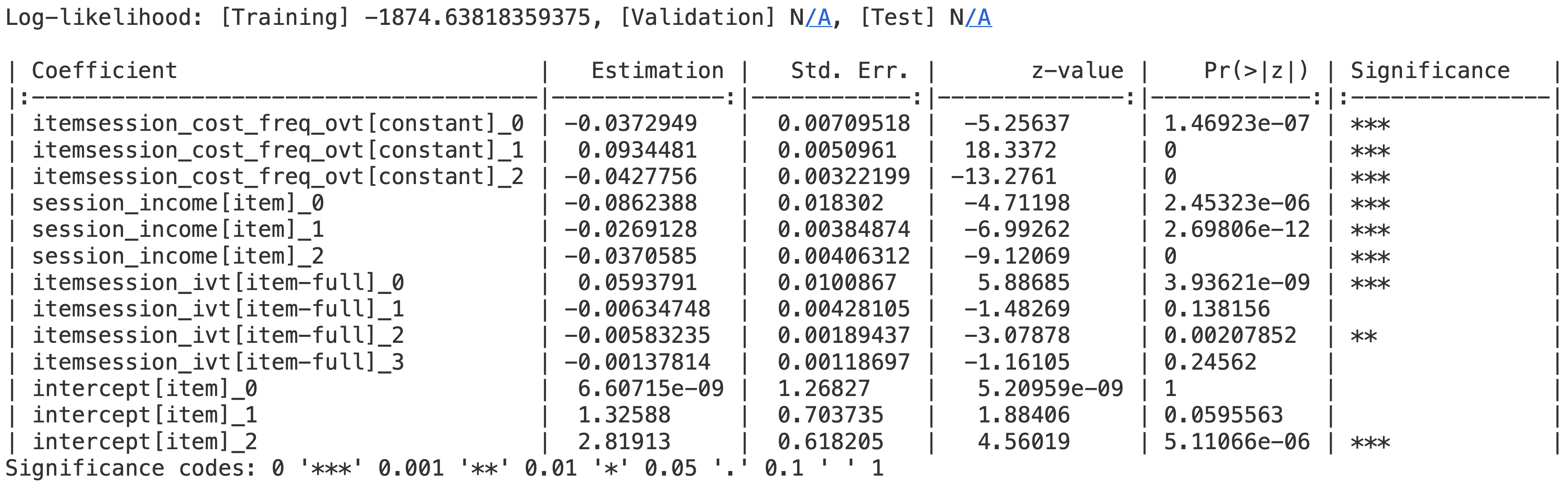
Figure 2: Coefficient Estimation Table from run() Function Call

After the model estimation begins, torch-choice creates a TensorBoard log to illustrate the training progress; researchers can start a TensorBoard using the following command to obtain training progress like in Figure 3.

⬇

1tensorboard --logdir ./lightning_logs --port 6006

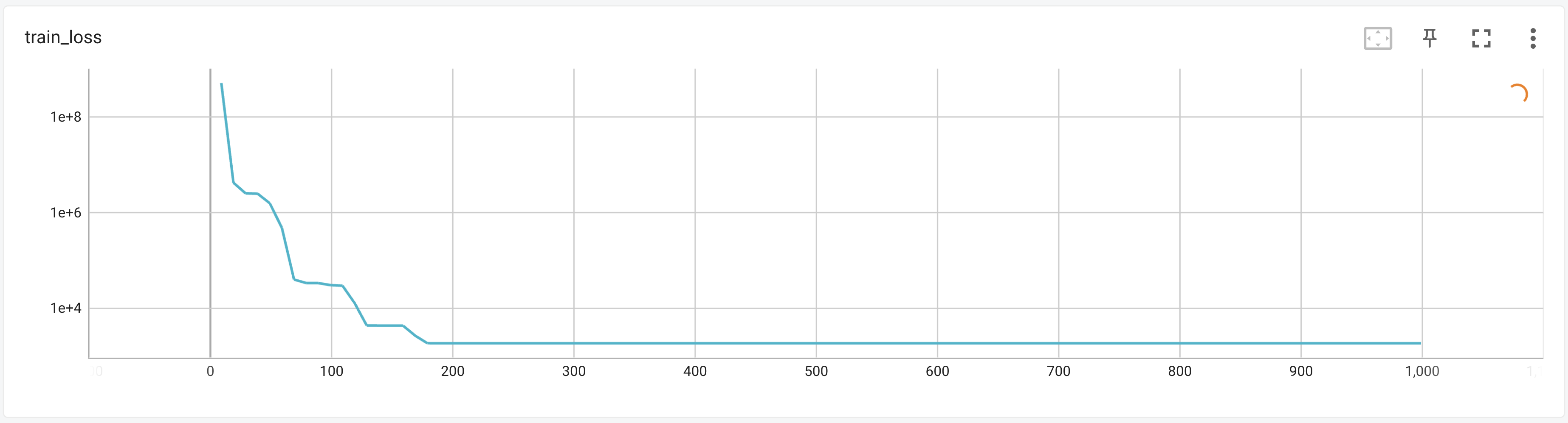
Figure 3: Training Progress Curve in TensorBoard

4.1.5 Post-Estimation

The torch-choice package provides utilities to help researchers easily retrieve estimated coefficients from fitted models. Consider the following stylized model configured with the code block.

$$\mu_{uis}=\alpha+\beta_{i}+\gamma_{u}+\delta_{i}^{\top}\textbf{x}^{(user)}_{u}+\eta^{\top}\textbf{y}^{(item)}_{i}+\theta_{u}^{\top}\textbf{z}^{(session)}_{s}+\kappa_{i}^{\top}\textbf{w}^{(itemsession)}_{is}+\iota_{u}^{\top}\textbf{w}^{(itemsession)}_{is}$$ (16)

⬇

1model = ConditionalLogitModel(

2 formula="(1|constant) + (1|item) + (1|user) + (user_obs|item) + (item_obs|constant) + (session_obs|user) + (itemsession_obs|item) + (itemsession_obs|user)",

3 dataset=dataset,

4 num_users=num_users,

5 num_items=num_items)

After the model estimation, the get_coefficient() method allows researchers to retrieve the coefficient values from the model using the general syntax model.get_coefficient(COEFFICIENT_NAME) with COEFFICIENT_NAME from the formula string. For example,

• model.get_coefficient("intercept[constant]") will return the estimated value of $\alpha$, which is a scalar.

• model.get_coefficient("intercept[user]") returns the array of $\gamma_{u}$’s, which is a 1D array of length num_users.

• model.get_coefficient("session_obs[user]") returns the corresponding coefficient $\theta_{u}$, which is a 2D array of shape (num_users, num_session_features). Each row of the returned tensor corresponds to the coefficient vector of a user.

Researchers can refer to our online documentation Tutorial: Conditional Logit Model on ModeCanada Dataset for a complete Jupyter Notebook tutorial.

4.2 Nested Logit Model

When items can naturally be clustered into nests, the nested logit model becomes a suitable option. The nested logit model assumes a weaker version of independence of irrelevant alternatives (IIA): the IIA assumption holds for each pair of items belonging to the same nest but not for pairs from different nests.

4.2.1 Model Specification

We implement a two level nested logit model, where at the higher nesting level the user chooses one of many nests, and at the lower level, the user chooses an item within a nest. Thus, the user selects exactly one item across all nests. In the current version of the software, the nested logit is available only in a setting where there is a single category. The nested logit model decomposes the utility of choosing item $i$ into the item-specific values and inclusive values for each nest as in Equation (18). This effectively allows correlation among the $\varepsilon_{uis}$ within the choices in a nest. Nests are indexed by $k\in\{1,2,\dots,K\}$, $\mathcal{K}(i)\in\{1,2,\dots,K\}$ denotes the nest of item $i$, and $I_{k}\subseteq\{1,2,\dots,I\}$ denotes the set of items in nest $k$. The NestedLogitModel constructor requires a nest_to_item dictionary mapping $k\mapsto I_{k}$, where keys of nest_to_item are nest indices $k$’s and nest_to_item[j] is a list consisting of item indices in $I_{k}$. Researchers do not need to supply a num_items argument to the NestedLogitModel class, the number of items is automatically inferred from the nest_to_item dictionary.

This section briefly discusses the derivation of the log-likelihood formula torch-choice maximizes. Researchers can refer to Discrete Choice Methods with Simulation by Kenneth Train for a more detailed treatment [33].

Let $\mathcal{V}_{uis}=\mu_{uis}+\varepsilon_{uis}$ denote the utility user $u$ gains from item $i$ in the context of session $s$. The NLM allows $\varepsilon_{uis}$ of items from the same nest to be correlated, but $\varepsilon_{uis}$ of items from different categories should be independent. The $\lambda_{k}$ denotes the degree of independence among $\varepsilon_{uis}$’s of items in nest $k$. Equation (17) illustrates the likelihood of item $i$ from the nested logit model.

$$P(i\mid u,s)=\frac{e^{\mu_{uis}/\lambda_{\mathcal{K}(i)}}\left(\sum_{j\in I_{\mathcal{K}(i)}}e^{\mu_{ujs}/\lambda_{\mathcal{K}(i)}}\right)^{\lambda_{\mathcal{K}(i)}-1}}{\sum_{k=1}^{K}\left(\sum_{j\in I_{k}}e^{\mu_{ujs}/\lambda_{k}}\right)^{\lambda_{k}}}$$ (17)

Without loss of generality, the utility $\mathcal{V}_{uis}$ can be decomposed into a nest-level component $W_{u\mathcal{K}(i)s}$ and an item-level component $T_{uis}$.

$$\mathcal{V}_{uis}=\mu_{uis}+\varepsilon_{uis}=W_{u\mathcal{K}(i)s}+T_{uis}+\varepsilon_{uis}$$ (18)

The likelihood in Equation (17) decomposes into a marginal probability of choosing nest $\mathcal{K}(i)$ and a conditional probability of choosing $i$ given nest $\mathcal{K}(i)$ is chosen.

$$P(i\mid u,s)=\underbrace{\frac{\exp\left(T_{uis}/\lambda_{\mathcal{K}(i)}\right)}{\sum_{j\in I_{\mathcal{K}(i)}}\exp\left(T_{ujs}/\lambda_{\mathcal{K}(i)}\right)}}_{\text{conditional prob. of item}}\underbrace{\frac{\exp\left(W_{u\mathcal{K}(i)s}+\lambda_{\mathcal{K}(i)}\mathcal{I}_{u\mathcal{K}(i)s}\right)}{\sum_{k=1}^{K}\exp\left(W_{uks}+\lambda_{k}\mathcal{I}_{uks}\right)}}_{\text{marginal prob. of nest}}$$ (19)

The inclusive value of nest $k$ (for user $u$ in session $s$), denoted as $\mathcal{I}_{uks}$, is defined as $\log\sum_{j\in I_{k}}\exp(T_{ujs}/\lambda_{k})$, which is the expected utility from choosing the best alternative from nest $k$ given Gumbel error term in utility.

The softmax form of marginal and conditional probabilities in Equation (19) suggests a way to model $\mathcal{V}$: estimate both $W_{u\mathcal{K}(i)s}$ and $T_{uis}$ using linear functional forms as in the conditional logit model with nest observables and item observables, respectively.

$$W_{uks} =\sum_{p=1}^{P}\bm{\theta}_{p}^{\top}\bm{x}_{p}$$ (20)

$$T_{uis} =\sum_{p=1}^{P^{\prime}}\bm{\gamma}_{p}^{\top}\bm{z}_{p}$$ (21)

where $\bm{\theta}_{p}$’s are coefficients of the nest-level model that can be (1) fixed for all items and users, (2) user-specific, and (3) item-specific (i.e., nest-specific since we are talking about the nest level model). $\bm{x}_{p}$’s are nest level observables. The nest-level model in NLM is similar to a CLM for choices over categories as items. The only difference between specifying the nest-level model and a CLM is that an item-specific coefficient or observable in the NLM nest-level model is indeed nest-specific. For example, by specifying nest_formula="(1|item)" for the nest-level model, the model specification in Equation (20) is $W_{uks}=\lambda_{c}$. $\bm{\gamma}_{p}$’s denote coefficients of item-level model and $\bm{z}_{p}$’s are item observables. Specification of the item-level model is exactly the same as in the CLM.

The configuration of NLM requires specifying both the item-level CLM and nest-level CLM. Similar to the CLM, researchers can configure models using Python dictionaries or R-like formulas. For example,

⬇

1nest_formula = ’(1|item) + (item_obs1|constant) + (session_obs1|user) + (user_obs1|item)’

2item_formula = ’(1|user) + (item_obs2|user) + (session_obs2|item) + (user_obs2|constant)’

specify the following model

$$W_{uks} =\tau_{k}+\beta^{\top}\bm{x}^{(\text{item obs 1})}_{k}+\gamma^{\top}_{u}\bm{x}^{(\text{session obs 1})}_{s}+\delta^{\top}_{k}\bm{x}^{(\text{user obs 1})}_{u}$$ (22)

$$T_{uis} =\alpha_{u}+\tau_{u}^{\top}\bm{x}^{(\text{item obs 2})}_{i}+\phi^{\top}_{i}\bm{x}^{(\text{session obs 2})}_{s}+\psi^{\top}\bm{x}^{(\text{user obs 2})}_{u}$$ (23)

It is worth mentioning that everything tagged with item in the nest_formula, such as item-specific intercepts/coefficients (i.e., (1|item) and (user_obs1|item)) and item-specific observables (i.e., (item_obs1|constant)) are indeed nest-specific with $k$ sub-script in Equation (22). For example, by specifying nest-level formula "(1|item)+(user_obs1|item)", it is interpreted as nest-specific fixed effect together with nest-specific random effect from user observable 1. Equivalently, $W_{uks}=\tau_{k}+\delta^{\top}_{k}\bm{x}^{(\text{user obs 1})}_{u}$.

Similar to specifying CLMs, researchers can use {nest, item}_coef_variation_dict and {nest, item}_num_param_dict to specify the functional form of $W_{uks}$ and $T_{uis}$ respectively.

Due to the decomposition in Equation (19), the log-likelihood for user $u$ to choose item $i$ in session $s$ can be written as Equation (24), and torch-choice jointly optimizes all coefficients to maximize Equation (24).

$$\log P(i\mid u,s) =\log P_{\text{item}}(i\mid u,s)+\log P_{\text{nest}}(\mathcal{K}(i)\mid u,s)$$ (24)

$$=\log\left(\frac{\exp(T_{uis}/\lambda_{k})}{\sum_{j\in I_{\mathcal{K}(i)}}\exp(T_{ujs}/\lambda_{k})}\right)+\log\left(\frac{\exp(W_{u\mathcal{K}(i)s}+\lambda_{\mathcal{K}(i)}\mathcal{I}_{u\mathcal{K}(i)s})}{\sum_{k=1}^{K}\exp(W_{uks}+\lambda_{k}\mathcal{I}_{uks})}\right)$$

torch-choice allows for empty nest-level models from an empty dictionary or empty formula string. In this case, $W_{uks}=\varepsilon_{uks}$ since the inclusive value term $\lambda_{k}I_{uks}$ will be used to model the choice over categories. In this special case, the model’s log-likelihood function reduces to Equation (25).

$$\log P(i\mid u,t)=\log\left(\frac{\exp(T_{uit}/\lambda_{k})}{\sum_{j\in B_{k}}\exp(T_{ujt}/\lambda_{k})}\right)+\log\left(\frac{\lambda_{k}\mathcal{I}_{ukt}}{\sum_{\ell=1}^{K}\lambda_{\ell}\mathcal{I}_{u\ell t}}\right)$$ (25)

However, by specifying an empty item-level model ($T_{uis}=\varepsilon_{uis}$), the nested logit model reduces to a conditional logit model of choices over categories. Hence, researchers should never use the NestedLogitModel class with an empty item-level model.

The $\lambda_{k}$’s capture the degree of independence among unobserved utilities $\varepsilon$ of items in nest $k$ [34]. torch-choice estimates $\lambda_{k}$’s jointly with other coefficients. By default, these paramaters differ over categories, indicating different levels of correlations among unobserved utilities of items in different categories. Researchers can specify shared_lambda=True to constrain $\lambda_{k}=\lambda$ for all categories, indicating the same level of correlations in all categories. Whether to add such a constraint is an empirical question depending on specific datasets; researchers can use hypothesis testing to determine the right configuration [33]. While working with large datasets, setting the same $\lambda$ for all categories helps reduce the number of parameters when the number of categories is potentially very large.

The following code snippets demonstrate the construction of nested logit models in torch-choice.

⬇

1# Creation of NestedLogitModel using formulas.

2model = NestedLogitModel(

3 nest_to_item=nest_to_item,

4 nest_formula=’(1|item) + (item_obs1|constant) + (session_obs1|user) + (user_obs1|item)’,

5 item_formula=’(1|user) + (item_obs2|user) + (session_obs2|item) + (user_obs2|constant)’,

6 dataset=dataset,

7 shared_lambda=True)

Similar to the CLMs, researchers can add $L^{1}$ or $L^{2}$ regularizations to NLMs by specifying regularization $\in$ {"L1", "L2"}and regularization_weight $\in\mathbb{R}_{+}$ keywords. For example, the following code creates a model that penalizes $\|\bm{\theta}\|_{2}$ during estimation.

⬇

1model = NestedLogitModel(regularization="L2", regularization_weight=1.5)

4.2.2 Dataset Preparation

The NestedLogitModel admits a JointDataset structure, which consists of separate ChoiceDataset objects holding observables for categories and items. Naming conventions for ChoiceDataset for item observables are exactly the same as before: researchers can specify item observables item_<obs_name>, user observables user_<obs_name>, session observables session_<obs_name>, and (item, session)-specific observables item_session_<obs_name>. For the dataset holding nest information, researchers need to add the item_index array $(i^{(n)})_{n=1}^{N}$, and all nest-specific observables should be named as item_<obs_name> because categories are considered as items in the nest-level model. Similarly, researchers can add (nest, session)-specific observables via the item_session_<obs_name> keyword. Lastly, the researcher can link two ChoiceDataset objects using the JointDataset class as in the following code block.

⬇

1# create the nest-level dataset.

2nest_dataset = ChoiceDataset(item_index=item_index, item_obs=..., use_obs=...)

3# create the item-level dataset.

4item_dataset = ChoiceDataset(item_index=item_index, item_obs=..., use_obs=...)

5# create the joint dataset.

6dataset = JointDataset(nest=nest_dataset, item=item_dataset)

4.2.3 Optimization and Model Estimation

For NLM estimation, torch-choice maximizes the likelihood defined in Equation (17) by updating all coefficients iteratively using optimization algorithms like stochastic gradient descent. To estimate NLM, researchers need to provide a joint dataset encompassing both nest and item-level datasets. The run() helper function works for NLM and joint datasets.

⬇

1from torch_choice import run

2# create the nest-level dataset.

3nest_dataset = ChoiceDataset(item_index=item_index.clone())

4# create the item-level dataset.

5item_dataset = ChoiceDataset(item_index=item_index, price_obs=price_obs)

6# create the joint dataset.

7dataset = JointDataset(nest=nest_dataset, item=item_dataset)

8# estimate the model.

9run(model, dataset, learning_rate=0.01, num_epochs=5000, model_optimizer="Adam")

Similar to the conditional logit model, researchers can specify regularization on coefficients by passing regularization and regularization_weight into the run() method.

Researchers can refer to our online documentation here - Random Utility Model (RUM) Part II: Nested Logit Model for complete tutorials on applying various NLM to the Heating and Cooling System Choice in Newly Built Houses in California dataset [33].

4.2.4 Post-Estimation

The nested logit model has a similar interface for coefficient extraction to the conditional logit model demonstrated above. Consider a nested logit model consisting of an item-level model in Equation (16) and a nest-level model incorporating user-fixed effect, category-fixed effect (i.e., specified by (1|item) in the nest_formula), and the user-specific coefficient on a 64-dimensional nest-specific observable (i.e., specified by (item_obs|user) in the nest_formula).

⬇

1nested_model = NestedLogitModel(

2 nest_to_item=nest_to_item,

3 nest_formula=’(1|user) + (1|item) + (item_obs|user)’,

4 item_formula=’(1|constant) + (1|item) + (1|user) + (user_obs|item) + (item_obs|constant) + (session_obs|user) + (itemsession_obs|item) + (itemsession_obs|user)’,

5 num_users=num_users,

6 dataset=joint_dataset,

7 shared_lambda=False)

Researchers need to retrieve the coefficients of the nested logit model using the get_coefficient() method with an additional level argument.

For example, researchers can use the following code snippet to retrieve the coefficient of the user-fixed effect in the nest-level model, which is a vector with num_users elements.

⬇

1nested_model.get_coefficient("intercept[user]", level="nest")

With level="item", the researcher can obtain the coefficient of user-specific fixed effect in the item level model (i.e., $\gamma_{u}$’s in Equation (16)), which is a vector with length num_users.

⬇

1nested_model.get_coefficient("intercept[user]", level="item")

Such API generalizes to all other coefficients listed above, such as itemsession_obs[item] and itemsession_obs[user]. One exception is the coefficients for inclusive values (often denoted as $\lambda$). Researchers can retrieve the coefficient of the inclusive value by using get_coefficient("lambda") without specifying the level argument. In fact, get_coefficient will disregard any level argument if the coefficient name is lambda. The returned value is a scalar if shared_lambda=True, and a 1D array of length num_nests if shared_lambda=False.

5 Performance

Leveraging parallel processors in modern graphical processing units (GPU), the torch-choice package is particularly efficient when we have many parameters. For example, estimating the item-specific slope $\beta_{i}^{(2)}$ in Equation (13) becomes computationally expensive when we have a large number of items. This section examines the computational efficiency of torch-choice as the dataset grows larger in different dimensions. For the analysis in this section, we simulate a retail choice dataset that aims to characterize a consumer choice in a supermarket. Our simulation script can be found here; a dataset like the one we used can be simulated using this script, please refer to our GitHub repository for more details. The simulated dataset includes 1,750,100 choice records from 500 users and 500 items; each user ($u$) and item ($i$) is associated with a 30-dimensional vector of characteristics generated randomly, denoted as $X_{u}\in\mathbb{R}^{30}$ and $Z_{i}\in\mathbb{R}^{30}$ respectively. There is no session-specific observable. We consider the models in Equations (26) to (28) to cover model specifications with and without random effects.

$$\mu_{uis} =\bm{\beta}^{\top}Z_{i}$$ (26)

$$\mu_{uis} =\bm{\alpha}_{i}^{\top}X_{u}$$ (27)

$$\mu_{uis} =\bm{\alpha}_{i}^{\top}X_{u}+\bm{\beta}^{\top}Z_{i}$$ (28)

As a convention, the coefficient of the first item $\bm{\alpha}_{0}$ is set to zero.

Experiments in this section demonstrate the scalability of torch-choice when researchers expand (1) the number of choice records (i.e., size of dataset), (2) the dimension of user/item covariates, and (3) the cardinality of the item set. For each of these, and for each specification above, two sets of experiments are conducted: (1) we compare the performance of torch-choice and an open source implementation, mlogit implemented in R, on datasets with small-to-medium sizes; (2) we examine the performance of torch-choice when we expand to even larger datasets. We run each of these benchmarks five times and compare average run times across five trials.

5.1 Scalability with Number of Records

The first set of experiments focuses on the performance of torch-choice as the number of records ($N$) grows while dimensions of user/item observables and the item set remain the same.

5.1.1 Comparison on Small Datasets

We sampled $30$ items and only used the first 10 dimensions in user and item characteristics through this experiment. The top panels in Figure 4 show the time cost of torch-choice as the number of records $N$ grows from 1,000 to 100,000. The vertical axis shows the ratio between the time taken at each level of $N$ and the baseline time cost at $N=1,000$. The R-implementation scales linearly as $N$ grows, and the runtime increases by 140x as the sample size rises by 100x for all three model configurations. Similar to mlogit, the runtime of torch-choice scales linearly as $N$ increases, but torch-choice is more computationally efficient as the cost rises by 1x$\sim$4x depending on model specification when the sample size increases by 100x.

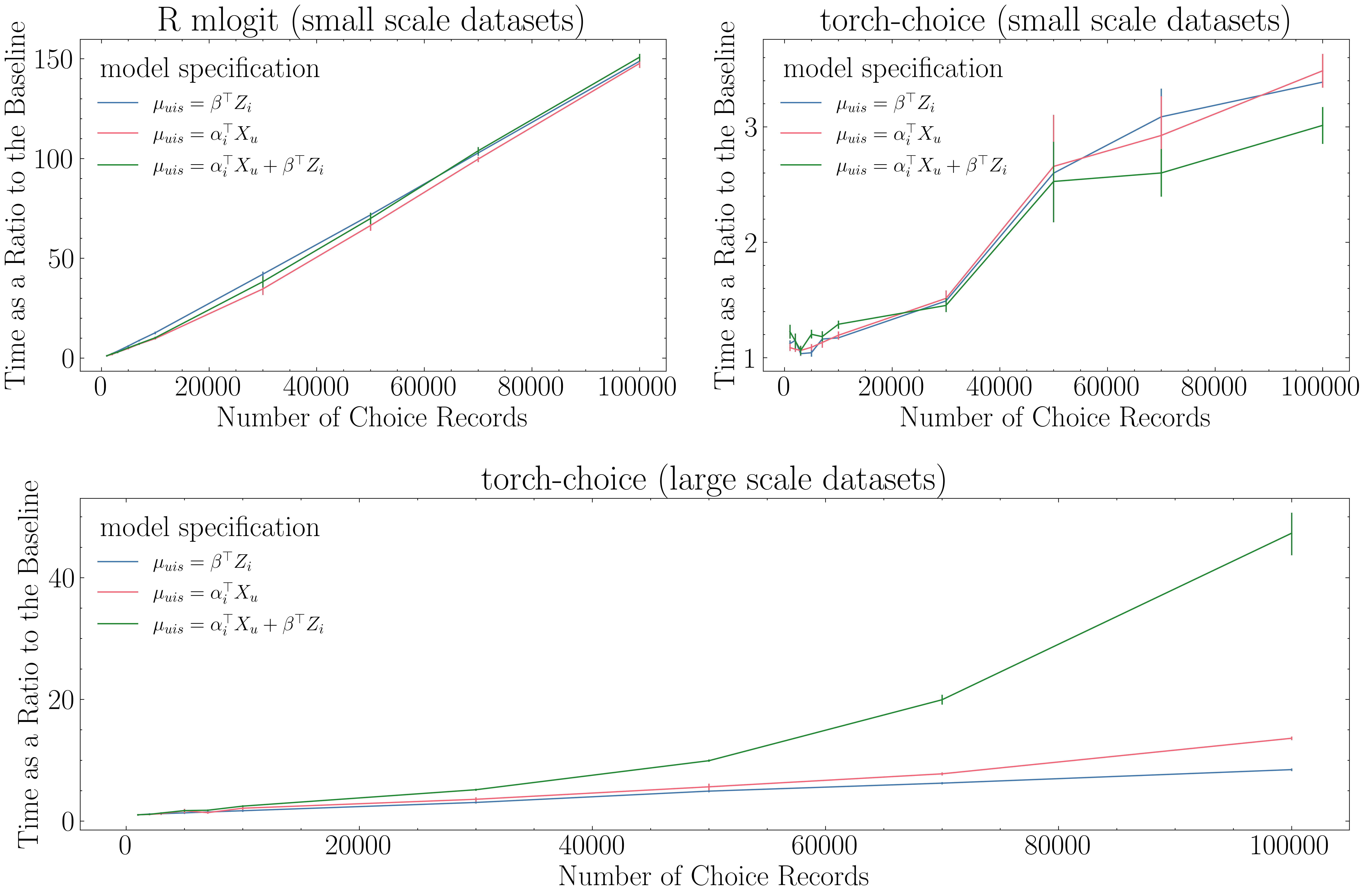
Figure 4: Time Cost Relative to Baseline Case as the Number of Records $N$ Rises

5.1.2 Performance on Larger Datasets

We then turn to the complete dataset with $500$ items and $30$-dimensional user/item characteristics. The bottom panel in Figure 4 illustrates the time taken relative to the baseline case ($N=1,000$) as $N$ increases from $1,000$ to $100,000$. The runtime of model (26) becomes vastly different from the other two because models with random effects now have 500x more parameters than model (26). The linear cost of torch-choice is preserved on the large-scale dataset, which provides evidence of scalability.

Finally, Figure 5 depicts the time cost in seconds of mlogit and torch-choice on different datasets. The Figure illustrates that in these datasets, torch-choice provided up to a 50x reduction in time.

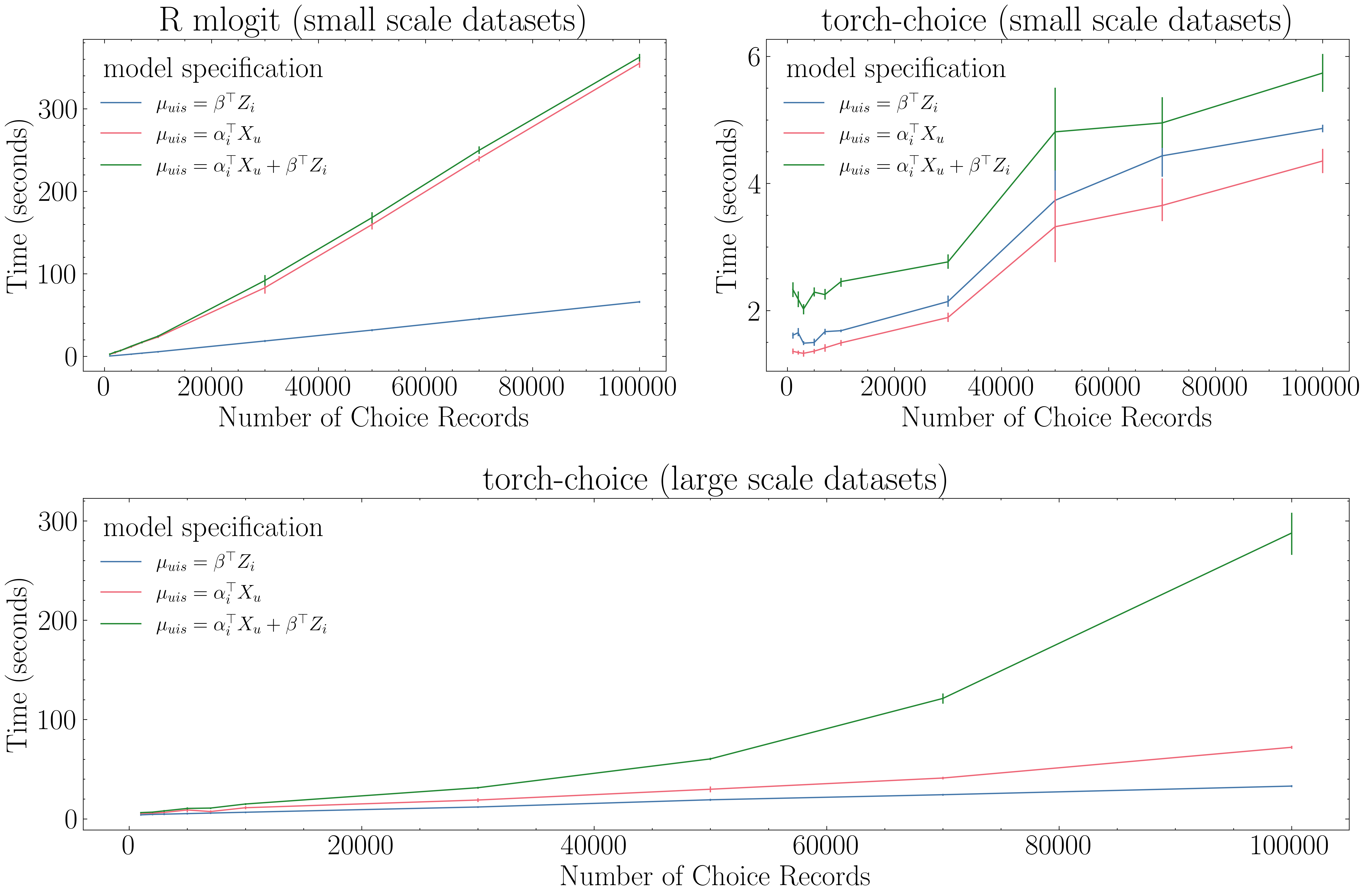
Figure 5: Time Cost (in Seconds) as the Number of Records $N$ Rises

5.2 Scalability with Number of Covariates

The number of parameters plays an important role in computational efficiency; as the number of parameters grows, the time cost of computing the gradient of the likelihood function also grows. In this section, we examine the performance of torch-choice as the number of covariates grows. We investigate the models in Equations (26) to (28) using only the first $P\in\{1,5,10,15,20,30\}$ dimensions of $X_{u}$ and $Z_{i}$.

5.2.1 Comparison on Small Datasets

The first part examines different packages’ time costs at each level of $P$ normalized by the baseline runtime ($P=1$) on a dataset with $N=10,000$ records and $I=50$ items. The top panels of Figure 6 compare computational efficiencies of R and torch-choice as the number of covariates grows. The time taken is more than 20x higher when $P=30$ compared to the baseline case while using the R-implementation; in contrast, the time cost is only doubled as $P$ increases with torch-choice.

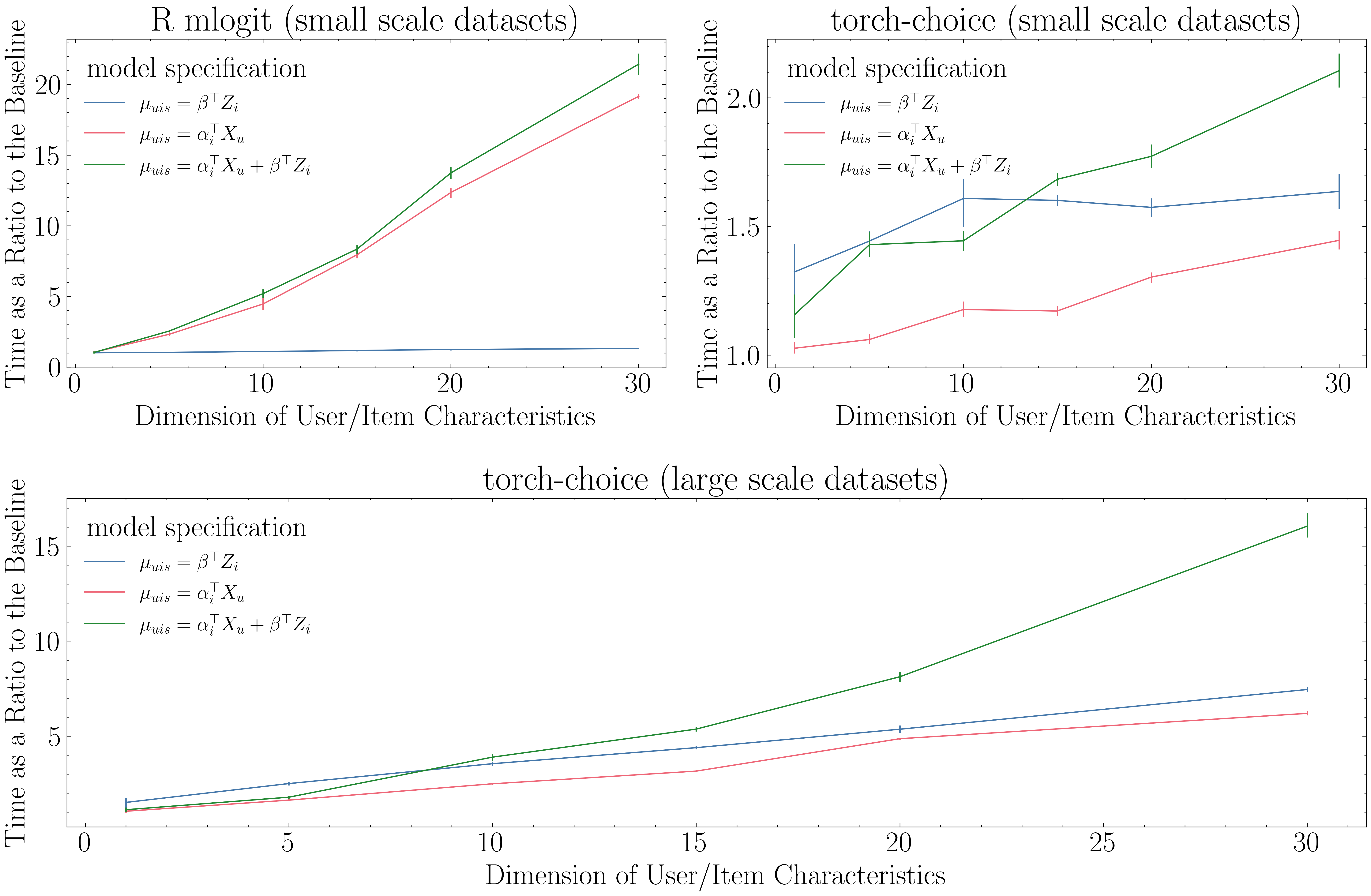
Figure 6: Time Cost Relative to Baseline Case as the Number of Covariates $P$ Rises

5.2.2 Performance on Larger Datasets

The bottom panel of Figure 6 illustrates the run time with different $P$’s on the large-scale dataset with $1,750,100$ records, $500$ users/items, and 30 user/item covariates. Model (28) with both random and common coefficients scaled worse than linear scaling, the run time increased by 15x when $P=30$. The scaling factor in time cost as $P$ expands depends on the number of items, which we will explore later, partly because the total number of parameters is $\mathcal{O}(P\times I)$. To summarize, torch-choice scales well when the number of items is moderate. Researchers should use caution while specifying item-specific random effects on high dimensional covariates when many items are present.

Finally, Figure 7 compares time cost in seconds of R and torch-choice in various scenarios, in which torch-choice delivers up to 100x speed-up compared to mlogit.

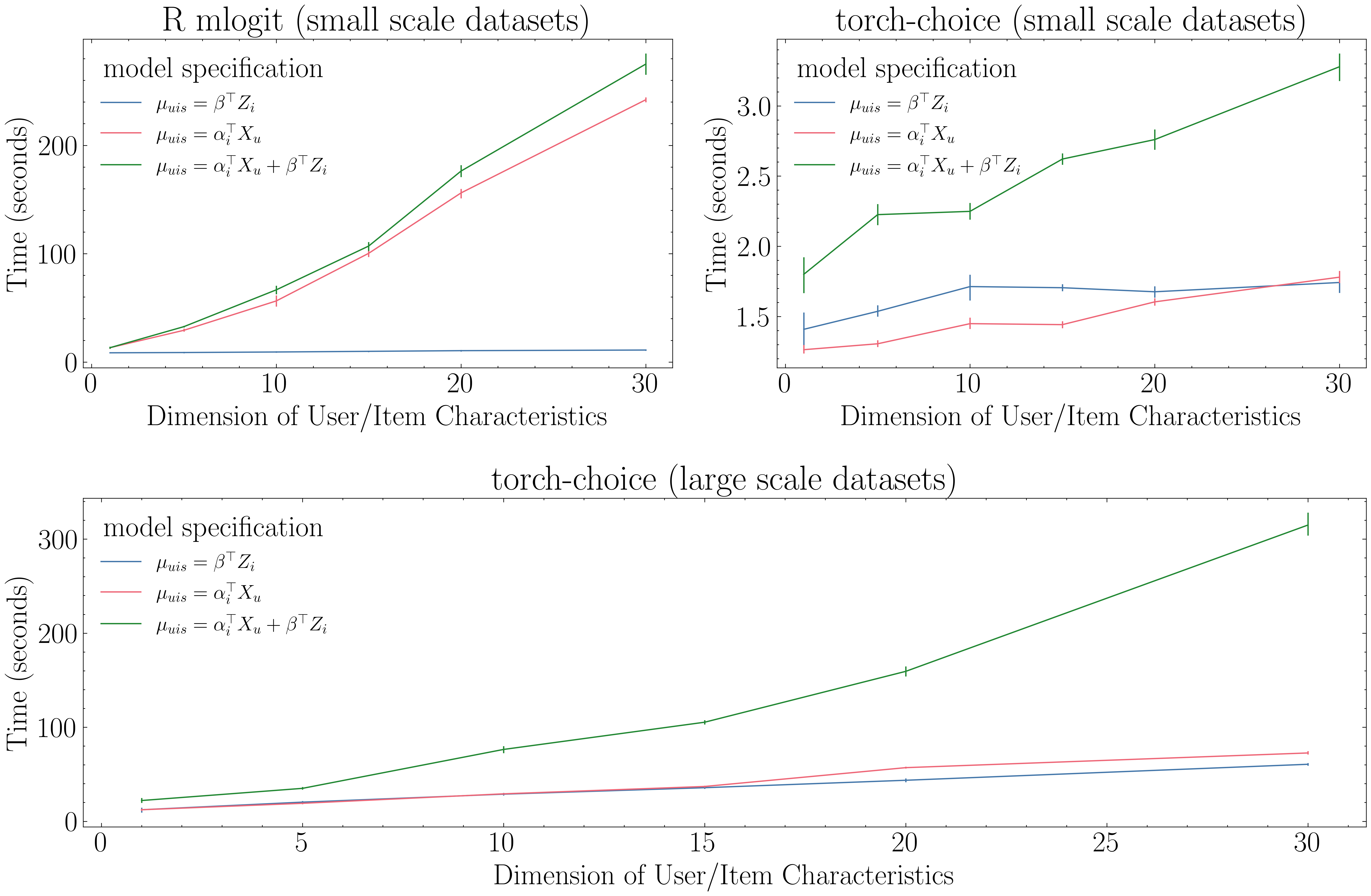
Figure 7: Time Cost (in Seconds) as the Number of Covariates $P$ Rises

5.3 Scalability with Number of Items

5.3.1 Comparison on Small Datasets

The number of parameters grows as the item set expands as well when item-specific coefficients are specified. In this section, we examine the performance of torch-choice as the number of items grows. We first compare performances, in terms of time cost relative to baseline case ($I=10$), of torch-choice and R-implementation as $I$ increases from $10$ to $200$ on a dataset with $N=30,000$ records and 30-dimensional user/item characteristics. We investigate the models in Equations (26) and (28), (27).

The top panels in Figure 8 show the time cost of torch-choice and mlogit as the number of items $I$ grows. Since the complexity of model (27) does not depend on the number of items, its cost grows slowly, only as a function of increased data size, and remains relatively constant as the number of items grows. torch-choice exhibits a linear runtime trend as $I$ grows, and costs of model (26) and model (28) are 2x and 6x higher when the number of items increases by 20x (from 10 to 200). In contrast, the curvatures in the left panel suggest an exponential growth trend in the time cost of mlogit; the computational cost required explodes by more than 300x when the number of items rises by 20x.

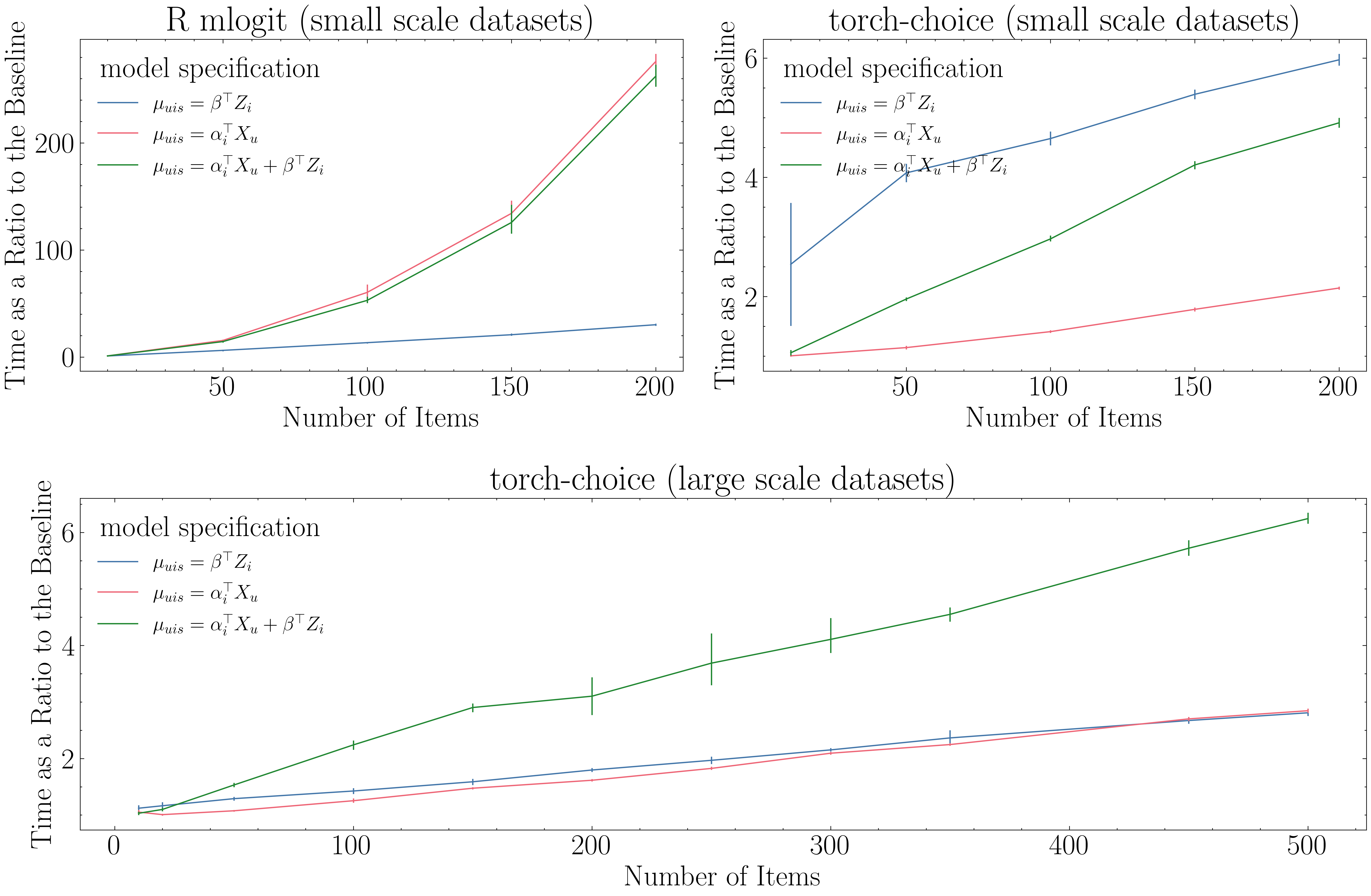
Figure 8: Time Cost Relative to Baseline Case as the Number of Items $I$ Rises

5.3.2 Performance on Larger Datasets

The bottom panel in Figure 8 demonstrates the runtime of torch-choice as $I$ increases up to 500. As we expected, the cost of estimating model (27) grows very slowly as we expand the item set. The computational costs at $I=500$ of both model (26) and model (28) rise by 2x and 6x, respectively, compared to $I=10$ (and are doubled compared to $I=200$). This provides further evidence that the computational cost using torch-choice obeys a linear trend with the expansion of the item set, which demonstrates torch-choice’s scalability.

Lastly, Figure 9 demonstrates the run time of torch-choice and mlogit in seconds through experiments considered in this section.

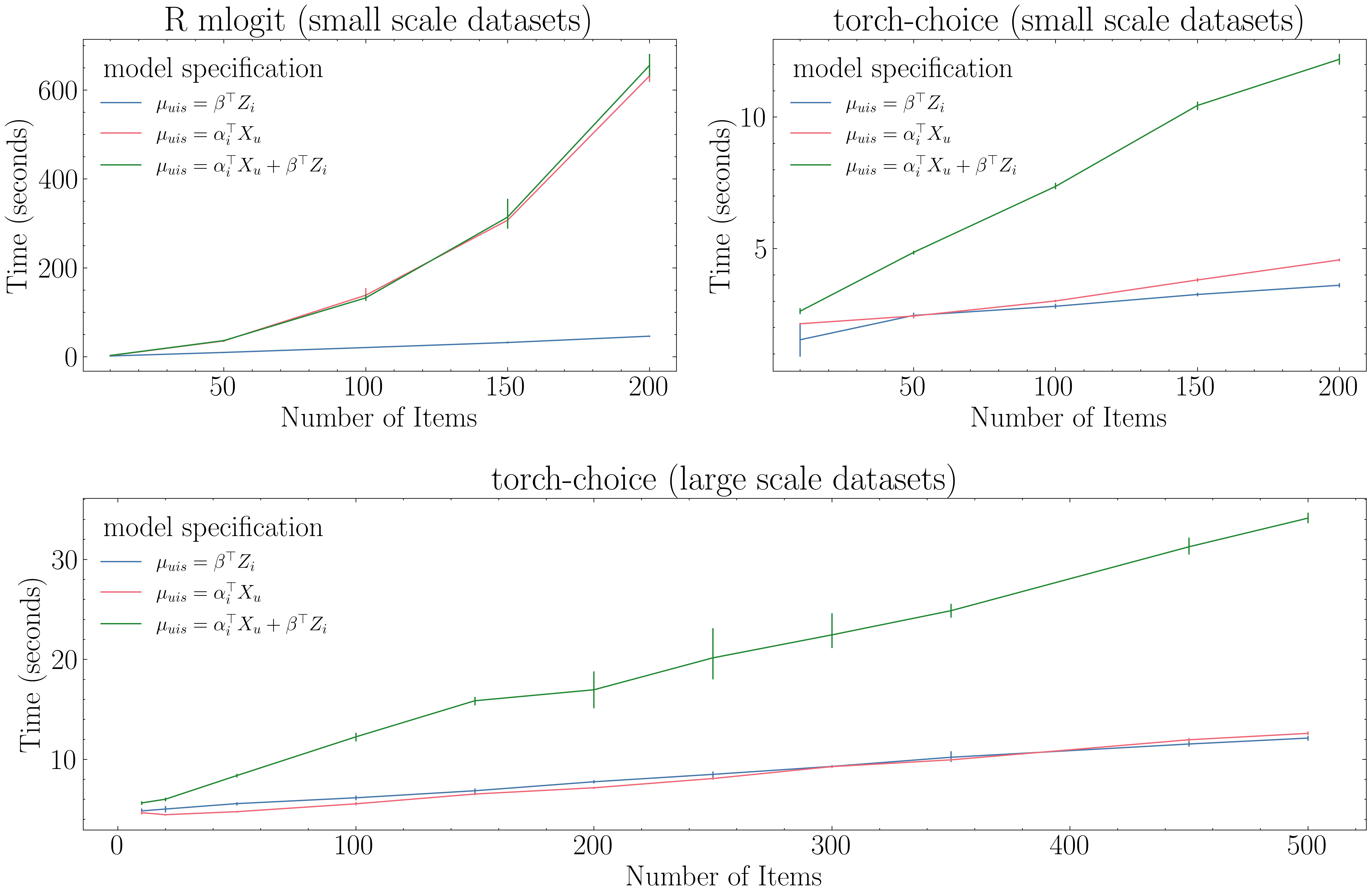
Figure 9: Time Cost (in Seconds) as the Number of Items $I$ Rises

6 Conclusion and Future Work

Choice modeling problems are ubiquitous in multiple disciplines, including Economics, Psychology, Education and Computer Science. As a result, access to effective choice modeling software is crucial for both researchers and practitioners. The torch-choice package aims to greatly improve this modeling landscape by providing a flexible and scalable choice modeling implementation.

In this paper, we proposed torch-choice, a PyTorch-based choice modeling package. The torch-choice package offers a memory-efficient data structure, ChoiceDataset for storing choice datasets. Towards this end, torch-choice also provides functionalities allowing researchers to build the ChoiceDataset, from databases in various formats. For the advanced user, the ChoiceDataset object is completely flexible and supports all functionalities in PyTorch’s dataset data structure.

The torch-choice package implements two widely-used classes of models, the ConditionalLogitModel and the NestedLogitModel using PyTorch. It allows researchers to fully specify flexible functional forms and changing item availability, which overcomes some of the difficulties when modeling with existing libraries. Models in torch-choice support regularization during model estimation, making it usable for engineering applications as well, a feature not provided in standard choice modeling libraries used by econometricians and statisticians. Such a feature vastly increases the scope of choice modeling options as compared to standard libraries used by engineers in terms of flexibility and scale.

The package has the advantage of scaling to massive datasets while being computationally efficient by using GPUs for estimation. We examined the scalability of mlogit in R and torch-choice while (1) increasing the number of observations, (2) increasing the number of covariates, and (3) expanding the item set with various model specifications. Experiment results show that torch-choice scales significantly better than R on small-to-medium-scale datasets. Then we test torch-choice on large-scale datasets that R cannot handle, on which torch-choice demonstrates its ability to scale up with computational efficiency.

Moving forward, we aim to maintain the reference implementation of torch-choice on the Python Package Index (PyPI) via Github, developing relatively few new features. We foresee the following important extensions to our models. First, torch-choice currently does not allow researchers to specify Bayesian priors over coefficients and learn posteriors instead of point estimates. With Bayesian coefficients, in addition to using item/user characteristics as observables, researchers can incorporate these characteristics into the coefficient prior and let them influence the coefficient posterior directly. Second, currently our nested logit model only supports two levels of nesting. Another direction is to implement multi-level nested logit models (i.e., nests within a nest), which are particularly useful when users make sequential decisions. In addition, allowing for modeling multiple categories with nested logit will be an important extension. We are actively developing these extensions and aim to release them soon.

References

- [1] Yves Croissant. Estimation of random utility models in r: The mlogit package. Journal of Statistical Software, 95(11):1–41, 2020.
- [2] Steven Berry, James Levinsohn, and Ariel Pakes. Automobile prices in market equilibrium. Econometrica: Journal of the Econometric Society, pages 841–890, 1995.
- [3] Steven Berry, James Levinsohn, and Ariel Pakes. Differentiated products demand systems from a combination of micro and macro data: The new car market. Journal of political Economy, 112(1):68–105, 2004.
- [4] Pradeep Chintagunta, Ekaterini Kyriazidou, and Josef Perktold. Panel data analysis of household brand choices. Journal of Econometrics, 103(1-2):111–153, 2001.
- [5] Daniel McFadden. The measurement of urban travel demand. Journal of public economics, 3(4):303–328, 1974.
- [6] Frank R Wilson, Sundar Damodaran, and J David Innes. Disaggregate mode choice models for intercity passenger travel in canada. Canadian Journal of Civil Engineering, 17(2):184–191, 1990.
- [7] Kazuaki Miyamoto, Varameth Vichiensan, Naoki Shimomura, and Antonio Páez. Discrete choice model with structuralized spatial effects for location analysis. Transportation Research Record, 1898(1):183–190, 2004.
- [8] Tom Kornstad and Thor O Thoresen. A discrete choice model for labor supply and childcare. Journal of Population Economics, 20(4):781–803, 2007.
- [9] Arthur Van Soest. Structural models of family labor supply: a discrete choice approach. Journal of human Resources, pages 63–88, 1995.
- [10] Frank B Baker. The basics of item response theory. ERIC, 2001.
- [11] Susan E Embretson and Steven P Reise. Item response theory. Psychology Press, 2013.
- [12] Thomas V Bonoma and Wesley J Johnston. Decision making under uncertainty: a direct measurement approach. Journal of Consumer Research, 6(2):177–191, 1979.
- [13] Joseph L Fleiss, Janet BW Williams, and Alan F Dubro. The logistic regression analysis of psychiatric data. Journal of Psychiatric Research, 20(3):195–209, 1986.
- [14] Tong Zhang and Vijay S Iyengar. Recommender systems using linear classifiers. The Journal of Machine Learning Research, 2:313–334, 2002.
- [15] Ming-wei Chang, Wen-tau Yih, and Christopher Meek. Partitioned logistic regression for spam filtering. In Proceedings of the 14th ACM SIGKDD international conference on Knowledge discovery and data mining, pages 97–105, 2008.
- [16] Li Deng. The mnist database of handwritten digit images for machine learning research [best of the web]. IEEE signal processing magazine, 29(6):141–142, 2012.
- [17] Susan Athey, David Blei, Robert Donnelly, Francisco Ruiz, and Tobias Schmidt. Estimating heterogeneous consumer preferences for restaurants and travel time using mobile location data. In AEA Papers and Proceedings, volume 108, pages 64–67, 2018.
- [18] Robert Donnelly, Francisco JR Ruiz, David Blei, and Susan Athey. Counterfactual inference for consumer choice across many product categories. Quantitative Marketing and Economics, 19(3):369–407, 2021.
- [19] Francisco JR Ruiz, Susan Athey, and David M Blei. Shopper: A probabilistic model of consumer choice with substitutes and complements. The Annals of Applied Statistics, 14(1):1–27, 2020.
- [20] Robert Donnelly, Ayush Kanodia, and Ilya Morozov. Welfare effects of personalized rankings. Available at SSRN 3649342, 2022.
- [21] Keyon Vafa, Emil Palikot, Tianyu Du, Ayush Kanodia, Susan Athey, and David M Blei. Learning transferrable representations of career trajectories for economic prediction. arXiv preprint arXiv:2202.08370, 2022.
- [22] Anders Krogh and John Hertz. A simple weight decay can improve generalization. Advances in neural information processing systems, 4, 1991.
- [23] F. Pedregosa, G. Varoquaux, A. Gramfort, V. Michel, B. Thirion, O. Grisel, M. Blondel, P. Prettenhofer, R. Weiss, V. Dubourg, J. Vanderplas, A. Passos, D. Cournapeau, M. Brucher, M. Perrot, and E. Duchesnay. Scikit-learn: Machine learning in Python. Journal of Machine Learning Research, 12:2825–2830, 2011.
- [24] Christopher Conlon and Jeff Gortmaker. Incorporating micro data into differentiated products demand estimation with PyBLP, 2023. Working paper.
- [25] Cristian Arteaga, JeeWoong Park, Prithvi Bhat Beeramoole, and Alexander Paz. xlogit: An open-source python package for gpu-accelerated estimation of mixed logit models. Journal of Choice Modelling, 42:100339, 2022.
- [26] Diederik P Kingma and Jimmy Ba. Adam: A method for stochastic optimization. arXiv preprint arXiv:1412.6980, 2014.
- [27] Dong C Liu and Jorge Nocedal. On the limited memory bfgs method for large scale optimization. Mathematical programming, 45(1-3):503–528, 1989.
- [28] William Falcon et al. Pytorch lightning. GitHub. Note: https://github. com/PyTorchLightning/pytorch-lightning, 3(6), 2019.
- [29] Maja Rudolph, Francisco Ruiz, Susan Athey, and David Blei. Structured embedding models for grouped data. Advances in neural information processing systems, 30, 2017.
- [30] Thomas Kluyver, Benjamin Ragan-Kelley, Fernando Pérez, Brian Granger, Matthias Bussonnier, Jonathan Frederic, Kyle Kelley, Jessica Hamrick, Jason Grout, Sylvain Corlay, Paul Ivanov, Damián Avila, Safia Abdalla, and Carol Willing. Jupyter notebooks – a publishing format for reproducible computational workflows. In F. Loizides and B. Schmidt, editors, Positioning and Power in Academic Publishing: Players, Agents and Agendas, pages 87 – 90. IOS Press, 2016.
- [31] Daniel McFadden et al. Conditional logit analysis of qualitative choice behavior. 1973.
- [32] Chandra R Bhat. A heteroscedastic extreme value model of intercity travel mode choice. Transportation Research Part B: Methodological, 29(6):471–483, 1995.
- [33] Kenneth E Train. Discrete choice methods with simulation. Cambridge university press, 2009.
- [34] Kenneth Train and Daniel McFadden. The goods/leisure tradeoff and disaggregate work trip mode choice models. Transportation research, 12(5):349–353, 1978.