Uncertainty Quantification for Recursive Estimation
in Adaptive Safety-Critical Control

Abstract

In this paper, we present a framework for online parameter estimation and uncertainty quantification in the context of adaptive safety-critical control. First, we demonstrate how incorporating a history stack of data into the classic recursive least squares algorithm facilitates parameter convergence under relaxed excitation conditions. Our key observation is that the estimate generated by this algorithm at any point in time is an affine transformation of the initial estimate. This property allows for parameterizing the uncertainty associated with such estimates using objects that are closed under affine transformation, such as zonotopes and Gaussian distributions, and enables the efficient propagation of such uncertainty metrics along the trajectory of the parameter estimates. We illustrate how such an approach facilitates the synthesis of safety-critical controllers for systems with parametric uncertainty using control barrier functions. Finally, we demonstrate the advantages of online adaptation and uncertainty quantification via numerical examples.

I Introduction

As autonomous systems are deployed in complex environments, it is essential for such systems to adapt to uncertainties that may be challenging to characterize until deployment. Recently, there has been a surge of interest in using data-driven and learning-based techniques to endow such systems with adaptive capabilities. This integration of learning and control, however, raises questions regarding the reliability and safety of such learning-enabled systems. In a control-theoretic context, simultaneous learning and control is the focus of adaptive control [1, 2] where the primary objective has been the stabilization of dynamical systems with parametric uncertainties. Such control designs are often carried out using Lyapunov-based tools, such as adaptive control Lyapunov functions [2], which guarantee stability by guiding parameter adaptation towards satisfaction of Lyapunov conditions. Although such approaches guarantee stability by construction, convergence of the parameter estimates to their true values (i.e., learning) is generally not achieved – classically, this is only guaranteed under persistence of excitation (PE) conditions that require the system trajectory to be sufficiently excited for all time [1].

Although adaptive control schemes with strong stability guarantees have existed for decades, there has been much less work on extending such ideas to address other important properties, such as safety. More recently, the fundamental property of safety – informally thought of as requiring a system to “never do anything bad” – has been formalized using the notion of set invariance [3]. In an analogous fashion to how Lyapunov functions are leveraged to certify the stability of equilibrium points without integrating a system’s vector fields, the concept of a barrier function [4] provides a methodology to certify set invariance without computing a system’s reachable set. Such ideas naturally extend to control systems via control barrier functions (CBFs) [3, 4] that allow for the design of controllers that enforce set invariance.

Given the duality between Lyapunov and barrier functions [3], and motivated by the need to develop certifiably correct learning-based control techniques, recent works have begun to transfer Lyapunov-based adaptive control techniques to a barrier function setting. For example, [5] introduced the notion of an adaptive CBF (aCBF) that allows for synthesizing controllers and parameter update laws enforcing set invariance conditions for nonlinear systems with uncertain parameters. A key insight of follow-up works [6, 7, 8, 9, 10, 11, 12] is that directly extending classical Lyapunov-based techniques to a barrier function setting can lead to overly conservative controllers and that such conservatism can be reduced by taking a robust adaptive control approach. Here, one often assumes known bounds on the system parameters, designs a robust controller enforcing safety for all possible realizations of the parameters, and then reduces the robustness of this controller as the uncertainty in the parameter estimates shrinks. Many of these approaches rely on various uncertainty quantification mechanisms associating an uncertainty metric to a given parameter estimate. In [6, 13] uncertainty quantification is achieved using set membership identification (SMID), which maintains a feasible set of parameter values consistent with the data observed up to the current time. Other works [7, 8] leverage techniques from concurrent learning – a data-driven adaptive control method [14, 15] – to provide verifiable bounds on the parameter estimation error. Other techniques such as Bayesian linear regression (BLR) [16] and Gaussian process regression [17, 18] have also been used for online adaptation and uncertainty quantification in a barrier setting. We note that although the focus of this paper is on barrier functions, similar online adaptation and uncertainty quantification techniques have been applied within other safety-critical control frameworks such as model predictive control [19, 20] and Hamilton-Jacobi reachability [21].

In this paper, we unite the aforementioned ideas to present a flexible framework for online parameter estimation and uncertainty quantification in the context of adaptive safety-critical control. Our starting point is the classic recursive least squares (RLS) algorithm for online parameter estimation. Inspired by [14], we demonstrate how incorporating a history stack of data into RLS facilitates parameter convergence under milder conditions than the traditional PE condition (Sec. III). The key property of RLS that we exploit for uncertainty quantification is that the optimal parameter estimate at any point in time is an affine transformation of the initial estimate (Sec. IV). This affine property allows for parameterizing the uncertainty using various objects that are closed under affine transformation – in this paper, we leverage zonotopes [22] (Sec. IV-A) and Gaussian distributions (Sec. IV-B). Using zonotopes, our method results in a recursive SMID technique whose computations only require performing affine transformations rather than solving optimization problems such as in [6, 13, 20]. Using Gaussians, our method results in a recursive BLR technique that avoids online matrix inversions, such as in [16], and relies on a relaxed version of the PE condition assumed in [19]. We demonstrate how both of these approaches facilitate the synthesis of safety-critical controllers for nonlinear systems with parametric uncertainties using CBFs (Sec. V). Finally, we demonstrate the benefits of online adaptation and uncertainty quantification via numerical examples (Sec. VI).

II Preliminaries and Problem Formulation

Notation: Given a matrix $A\in\mathbb{R}^{n\times n}$ the notation $A\geq 0$ ($A>0$) denotes that $A$ is positive semidefinite (positive definite). We use $I$ to denote an identity matrix of appropriate dimensions. Given matrices $A,B$ with the same number of rows, we use $[A,B]$ to denote their horizontal concatenation. Given a continuously differentiable function $h\,:\,\mathbb{R}^{n}\rightarrow\mathbb{R}$ and a vector field $f\,:\,\mathbb{R}^{n}\rightarrow\mathbb{R}^{n}$, we use $L_{f}h(x)\coloneqq\nabla h(x)^{\top}f(x)$ to denote the Lie derivative of $h$ along $f$. A continuous function $\alpha\,:\,\mathbb{R}\rightarrow\mathbb{R}$ is said to be an extended class $\mathcal{K}_{\infty}$ function, denoted by $\alpha\in\mathcal{K}_{\infty}^{e}$, if $\alpha(0)=0$, it is strictly increasing, $\lim_{r\rightarrow\infty}\alpha(r)=\infty$, and $\lim_{r\rightarrow-\infty}\alpha(r)=-\infty$. We use $\|\cdot\|$ and $\|\cdot\|_{\infty}$ to denote the Euclidean norm and infinity norm, respectively, and define $\|x\|_{A}\coloneqq x^{\top}Ax$ for a vector $x$ and matrix $A$ of appropriate dimensions. The notation $\mathcal{N}(\mu,\Sigma)$ represents a Gaussian distribution with mean $\mu$ and covariance $\Sigma$.

Barrier Functions: Consider the dynamical system

$$\dot{x}=f(x),$$ (1)

where $x\in\mathbb{R}^{n}$ is the system state and $f\,:\,\mathbb{R}^{n}\rightarrow\mathbb{R}^{n}$ is a locally Lipschitz vector field. Under this assumption, for any initial condition $x_{0}\in\mathbb{R}^{n}$, there exists a maximal interval of existence $\mathcal{I}=[0,\tau_{\max})$ and a unique continuously differentiable function $x\,:\,\mathcal{I}\rightarrow\mathbb{R}^{n}$ such that $x(\cdot)$ is a trajectory of (1) in the sense that it satisfies $x(0)=x_{0}$ and $\dot{x}(t)=f(x(t))$ for all $t\in\mathcal{I}$. The main property of (1) that we wish to certify is safety. Formally, (1) is said to be safe on a set $\mathcal{C}\subset\mathbb{R}^{n}$ if $\mathcal{C}$ is forward invariant, i.e., if $x(0)\in\mathcal{C}$, then $x(t)\in\mathcal{C}$ for all $t\in\mathcal{I}$. To provide convenient conditions for verifying safety properties of (1), we specialize the class of sets whose invariance we wish to certify to those that can be expressed as the zero superlevel set of a continuously differentiable function $h\,:\,\mathbb{R}^{n}\rightarrow\mathbb{R}$ as

$$\mathcal{C}=\{x\in\mathbb{R}^{n}\,:\,h(x)\geq 0\}.$$ (2)

Safety can be certified through the use of barrier functions.

Definition 1 ([4]).

A continuously differentiable function $h\,:\,\mathbb{R}^{n}\rightarrow\mathbb{R}$ is said to be a barrier function for (1) on a set $\mathcal{C}\subset\mathbb{R}^{n}$ as in (2) if $\nabla h(x)\neq 0$ for all $x\in\partial\mathcal{C}$ and there exists $\alpha\in\mathcal{K}_{\infty}^{e}$ such that for all $x\in\mathbb{R}^{n}$

$$\dot{h}(x)=\nabla h(x)^{\top}f(x)\eqqcolon L_{f}h(x)\geq-\alpha(h(x)).$$ (3)

The following theorem shows that the existence of a barrier function is sufficient to establish safety.

Theorem 1 ([4]).

If $h\,:\,\mathbb{R}^{n}\rightarrow\mathbb{R}$ is a barrier function for (1) on a set $\mathcal{C}\subset\mathbb{R}^{n}$ as in (2), then $\mathcal{C}$ is forward invariant.

The notion of a barrier function naturally extends to systems with inputs via control barrier functions (CBFs), which are, in essence, barrier function candidates that can be made to satisfy the criteria of Def. 1 via feedback control. A more formal definition of CBFs can be found in [3, 4].

Least Squares Regression: For much of this paper, we consider recursive least squares (RLS) techniques for regression in the context of estimating the parameters $\theta\in\mathbb{R}^{p}$ of a linear regression model of the form

$$y(t)=\Phi(t)\theta.$$ (4)

Here, $y\,:\,\mathbb{R}_{\geq 0}\rightarrow\mathbb{R}^{n}$ associates to each time a target vector and $\Phi\,:\,\mathbb{R}_{\geq 0}\rightarrow\mathbb{R}^{n\times p}$ associates to each time a regression matrix that encodes the relevant features for parameter estimation. In the context of this paper, the parameters in (4) will correspond to uncertain model parameters of a dynamical system that we wish to control; however, our approach applies to more general contexts as well.

III Recursive-Batch Least Squares Regression

In this section, we present a hybrid approach that combines aspects of batch and recursive least squares techniques for regression in the context of estimating the parameters $\theta\in\mathbb{R}^{p}$ of the regression model from (4). To develop such an approach we first introduce the idea of a history stack.

Definition 2.

A collection of tuples $\mathcal{H}(t)=\{(y_{j}(t),\Phi_{j}(t))\}_{j=1}^{M}$, where $y_{j}(\cdot)$, $\Phi_{j}(\cdot)$ are piecewise continuous, is said to be a history stack for (4) if $y_{j}(t)=\Phi_{j}(t)\theta$ for all $t\geq 0$ and all $j\in\{1,\dots,M\}$.

The notation $y_{j}(t)$ denotes the value of the target $y$ present in the $j$th slot of the history stack at time $t$, which may have been recorded as some previous instance $t_{k}\leq t$. That is, $y_{j}(t)=y(t_{k})$ for some $t_{k}\leq t$. The history stack may be initially empty, in which case we initialize all values to zero, or may be populated with data obtained from a previous experiment. The main idea behind our approach is to recursively estimate the parameters based upon the data present in $\mathcal{H}$, which is updated over time as more data is observed. As illustrated in this section, such an approach allows for efficiently estimating the parameters online while providing relatively mild conditions for parameter convergence. Our main objective is to compute an estimate of the parameters $\hat{\theta}$ that minimizes the following cost

$$J_{t}(\hat{\theta})=\frac{1}{2}\int_{0}^{t}\sum_{j=1}^{M}\|y_{j}(s)-\Phi_{j}(s)\hat{\theta}\|^{2}ds+\frac{1}{2}\|\hat{\theta}-\bar{\theta}_{0}\|_{\Sigma_{0}^{-1}}^{2},$$ (5)

parameterized by $t\in\mathbb{R}_{\geq 0}$, where $\bar{\theta}_{0}\in\mathbb{R}^{p}$ and $\Sigma_{0}\in\mathbb{R}^{p\times p}$ is a positive definite matrix. The first term in (5) attempts to minimize the total prediction error incurred up to time $t$, whereas the second accounts for prior knowledge of the parameters. For example, $\bar{\theta}_{0}$ and $\Sigma_{0}$ may represent the mean and covariance of a Gaussian prior placed on $\theta$ – such an idea will be made formal in proceeding sections. By taking the gradient of (5) and setting it equal to zero, one can show that the estimate $\hat{\theta}(t)$ minimizing (5) is given by

$$\hat{\theta}(t)=\Gamma(t)\bigg{[}\Sigma_{0}^{-1}\bar{\theta}_{0}+\int_{0}^{t}\sum_{j=1}^{M}\Phi_{j}(s)^{\top}y_{j}(s)ds\bigg{]},$$ (6a)

$$\Gamma(t)=\bigg{[}\Sigma_{0}^{-1}+\int_{0}^{t}\sum_{j=1}^{M}\Phi(s)^{\top}\Phi(s)ds\bigg{]}^{-1}.$$ (6b)

The form of (6) is somewhat inconvenient from an implementation standpoint as it requires computing various integrals and inverting a matrix for each $t$. The following lemma demonstrates that (6) can be efficiently computed by propagating forward a pair of differential equations.

Lemma 1.

The expressions for $\hat{\theta}$ and $\Gamma$ from (6a) and (6b), respectively, are the solutions to the initial value problems

$$\dot{\hat{\theta}}(t)=\Gamma(t)\sum_{j=1}^{M}\Phi_{j}(t)^{\top}\big{[}y_{j}(t)-\Phi_{j}(t)\hat{\theta}(t)\big{]},$$ (7a)

$$\dot{\Gamma}(t)=-\Gamma(t)\sum_{j=1}^{M}\Phi_{j}(t)^{\top}\Phi_{j}(t)\Gamma(t),$$ (7b)

with initial conditions $\hat{\theta}(0)=\bar{\theta}_{0}$ and $\Gamma(0)=\Sigma_{0}$.

Proof.

Follows the same steps outlined in [1, Ch. 4.3.6]. ∎

The following lemma shows that $\Gamma$ and the parameter estimation error $\tilde{\theta}\coloneqq\theta-\hat{\theta}$ are nonincreasing in time.

Lemma 2.

The update laws from (7) ensure that

• $\Gamma(t)$ is bounded as $0\leq\Gamma(t)\leq\Sigma_{0}$ for all $t\geq 0$;

• $\tilde{\theta}(t)$ is bounded as $\|\tilde{\theta}(t)\|\leq\|\tilde{\theta}(0)\|$ for all $t\geq 0$;

• $\tilde{\theta}(t)=\Gamma(t)\Sigma^{-1}_{0}\tilde{\theta}(0)$ for all $t\geq 0$.

Proof.

The update law from (7b) implies that $\dot{\Gamma}\leq 0$, which implies that $\Gamma(t)\leq\Gamma(0)=\Sigma_{0}$ for all $t\geq 0$. Since $\Sigma_{0}$ is positive definite it follows from (6b) that $\Gamma(t)^{-1}$ is positive definite for all finite $t\geq 0$, which implies $\Gamma(t)$ is positive definite for all finite $t\geq 0$. As $\Gamma(\cdot)$ is non-increasing and bounded from below, it has a limit $\Gamma_{\infty}\coloneqq\lim_{t\rightarrow\infty}\Gamma(t)$ as $t\rightarrow\infty$. Note that if $\lim_{t\rightarrow\infty}\int_{0}^{t}\sum_{j=1}^{M}\Phi_{j}(s)^{\top}\Phi_{j}(s)ds$ is unbounded then $\lim_{t\rightarrow\infty}\Gamma(t)^{-1}$ is unbounded as well and $\Gamma_{\infty}\in\mathbb{R}^{p\times p}$ may be positive semidefinite. To establish bounds on $\tilde{\theta}$, we note that

$$\frac{d}{dt}(\Gamma^{-1}\tilde{\theta})= \frac{d\Gamma^{-1}}{dt}\tilde{\theta}+\Gamma^{-1}\dot{\tilde{\theta}}$$ (8)

$$= \sum_{j=1}^{M}\Phi_{j}^{\top}\Phi_{j}\tilde{\theta}-\sum_{j=1}^{M}\Phi_{j}^{\top}[y_{j}-\Phi_{j}\hat{\theta}]$$

$$= \sum_{j=1}^{M}\Phi_{j}^{\top}\Phi_{j}\tilde{\theta}-\sum_{j=1}^{M}\Phi_{j}^{\top}\Phi_{j}\tilde{\theta}=0,$$

where the second equality follows from differentiating (6b), substituting in (7a), and using $\dot{\tilde{\theta}}=-\dot{\hat{\theta}}$. Integrating $\tfrac{d}{dt}(\Gamma^{-1}\tilde{\theta})$ over an interval $[0,t]$ yields $\Gamma^{-1}(t)\tilde{\theta}(t)=\Gamma^{-1}(0)\tilde{\theta}(0)=\Sigma^{-1}_{0}\tilde{\theta}(0)$, which implies

$$\tilde{\theta}(t)=\Gamma(t)\Sigma^{-1}_{0}\tilde{\theta}(0),$$ (9)

for all $t\geq 0$. Finally, using the fact that $\Gamma(t)\leq\Sigma_{0}$ for all $t\geq 0$, the above implies that

$$\|\tilde{\theta}(t)\|\leq\|\Gamma(t)\Sigma_{0}^{-1}\|\|\tilde{\theta}(0)\|\leq\|\Sigma_{0}\Sigma_{0}^{-1}\|\|\tilde{\theta}(0)\|= \|\tilde{\theta}(0)\|,$$

as desired. ∎

Although the preceding result establishes that the parameter estimation error is bounded and nonincreasing it does not establish under what conditions the estimates are guaranteed to converge to their true values. Classically, the condition required for convergence when using recursive estimation is the persistence of excitation (PE) condition [1], which is often impractical to achieve and is challenging to verify [14]. The following definition, based on the developments in [14], outlines a weaker condition for parameter convergence that depends on the data stored in a given history stack.

Definition 3.

A history stack is said to satisfy the finite excitation (FE) condition if there exists a $T\geq 0$ such that

$$\underline{\lambda}\coloneqq\inf_{t\geq T}\Bigg{[}\lambda_{\min}\bigg{(}\sum_{j=1}^{M}\Phi_{j}(t)^{\top}\Phi_{j}(t)\bigg{)}\Bigg{]}>0.$$ (10)

The preceding condition requires the existence of a time $T\geq 0$ such that $\sum_{j=1}^{M}\Phi_{j}(t)^{\top}\Phi_{j}(t)$ is positive definite for each $t\geq T$. Importantly, there exist algorithms for recording data so that $\lambda_{\min}(\sum_{j=1}^{M}\Phi_{j}(t)^{\top}\Phi_{j}(t))$ is non-increasing in time [15]; hence, if one can verify that the matrix is positive definite at a single instant in time, then one can verify the satisfaction of Def. 3. From a practical standpoint, Def. 3 can often be satisfied passively by storing diverse data in $\mathcal{H}$ over the normal course of system operation without having to take additional steps to excite the trajectory as is typical for the PE condition. The following theorem illustrates that Def. 3 is sufficient for parameter convergence.

Theorem 2.

Let $\mathcal{H}$ satisfy the FE condition. Then, the update laws in (7) guarantee that $\lim_{t\rightarrow\infty}\hat{\theta}(t)=\theta$.

Proof.

It follows from (9) that $\lim_{t\rightarrow\infty}\tilde{\theta}(t)=\Gamma_{\infty}\Sigma_{0}^{-1}\tilde{\theta}(0)$ where $\Gamma_{\infty}=\lim_{t\rightarrow\infty}\Gamma(t)$ was shown to exist in Lemma 2. It remains to show that $\Gamma_{\infty}=0$. Letting $t\geq T$, where $T\geq 0$ is from Def. 3, the expression for $\Gamma$ from (6b) implies

$$\Gamma(t)^{-1}= \Sigma_{0}^{-1}+\int_{0}^{T}\sum_{j=1}^{M}\Phi_{j}(s)^{\top}\Phi_{j}(s)ds$$

$$+\int_{T}^{t}\sum_{j=1}^{M}\Phi_{j}(s)^{\top}\Phi_{j}(s)ds,$$

which can be lower bounded as

$$\Gamma(t)^{-1}\geq \int_{T}^{t}\sum_{j=1}^{M}\Phi_{j}(s)^{\top}\Phi_{j}(s)ds$$

$$\geq \int_{T}^{t}\lambda_{\min}\bigg{(}\sum_{j=1}^{M}\Phi_{j}(s)^{\top}\Phi_{j}(s)\bigg{)}dsI$$

$$\geq \int_{T}^{t}\underline{\lambda}Ids=\underline{\lambda}(t-T)I,$$

where the first inequality follows from the fact that $\int_{0}^{T}\sum_{j=1}^{M}\Phi_{j}(s)^{\top}\Phi_{j}(s)ds$ is positive semidefinite and that $\Sigma_{0}^{-1}$ is positive definite and the third from the satisfaction of the FE condition. Hence,

$$\Gamma(t)\leq\tfrac{1}{\underline{\lambda}(t-T)}I,\quad\forall t\in[T,\infty).$$

As $t\rightarrow\infty$ the denominator in the above term also tends to infinity and thus $\lim_{t\rightarrow\infty}\Gamma(t)=\Gamma_{\infty}\leq 0$. Since $\Gamma_{\infty}\leq 0$ and $\Gamma_{\infty}\geq 0$ (by Lemma 2), we must have $\Gamma_{\infty}=0$, which implies that $\lim_{t\rightarrow\infty}\tilde{\theta}(t)=0$, as desired. ∎

IV RLS Uncertainty Quantification

In this section we demonstrate how the estimation scheme introduced in the previous section naturally extends to quantifying the uncertainty in the parameter estimate $\hat{\theta}$ through the matrix $\Gamma$. The motivation for taking such an approach stems from the use of the estimated parameters in safety-critical control, where we are generally not only interested in obtaining a point-wise estimate of the parameters but also in quantifying the uncertainty associated with such an estimate.

IV-A Robust Uncertainty Quantification

We begin by taking a purely robust approach where we assume with absolute certainty that the parameters lie in a known set. For reasons that will become clear shortly, we assume that such sets are represented as zonotopes, which are widely used for reachability analysis [22, 24].

Definition 4.

Given a center $c\in\mathbb{R}^{p}$ and generator $G\in\mathbb{R}^{p\times q}$, a zonotope is a set $\mathcal{Z}(c,G)\subset\mathbb{R}^{p}$ defined as

$$\mathcal{Z}(c,G)\coloneqq\left\{\theta\in\mathbb{R}^{p}\,:\,\theta=c+\sum_{i=1}^{q}\xi_{i}G_{i},\;\xi_{i}\in[-1,1],\;\forall i\right\},$$

where $\{G_{i}\}_{i=1}^{q}$ are the columns of $G$.

The main property of zonotopes we exploit is that they are closed under affine transformation [22]:

$$A\mathcal{Z}(c,G)+b=\mathcal{Z}(Ac+b,AG),$$ (11)

for a matrix $A$ and vector $b$ of appropriate dimensions. The primary observation that facilitates our extension of the previous estimation scheme to set-based estimates is that the point-wise estimate $\hat{\theta}(t)$ from (6a) at any given point in time is simply an affine transformation of the initial condition:

$$\hat{\theta}(t)= \underbrace{\Gamma(t)\Sigma_{0}^{-1}}_{A(t)}\bar{\theta}_{0}+\underbrace{\Gamma(t)\int_{0}^{t}\sum_{j=1}^{M}y_{j}(s)^{\top}\Phi_{j}(s)ds}_{b(t)}.$$ (12)

Replacing $\bar{\theta}_{0}$ with $\mathcal{Z}(\bar{\theta}_{0},\Sigma_{0})$ yields:

$$A(t)\mathcal{Z}(\bar{\theta}_{0},\Sigma_{0})+b(t)= \mathcal{Z}(A(t)\bar{\theta}_{0}+b(t),A(t)\Sigma_{0})$$ (13)

$$= \mathcal{Z}(\hat{\theta}(t),\Gamma(t)).$$

Further results are facilitated by the following lemma.

Lemma 3 ([25]).

Consider zonotopes $\mathcal{Z}(c_{1},G_{1})\subset\mathbb{R}^{p}$ and $\mathcal{Z}(c_{2},G_{2})\subset\mathbb{R}^{p}$ with centers $c_{1},c_{2}\in\mathbb{R}^{p}$ and generators $G_{1}\in\mathbb{R}^{p\times q}$, $G_{2}\in\mathbb{R}^{p\times r}$. Then, $\mathcal{Z}(c_{1},G_{1})\subseteq\mathcal{Z}(c_{2},G_{2})$ if there exists a pair $(z,P)\in\mathbb{R}^{p}\times\mathbb{R}^{r\times q}$ such that

$$G_{1}=G_{2}P$$ (14a)

$$c_{2}-c_{1}=G_{2}z$$ (14b)

$$\|[P,z]\|_{\infty}\leq 1.$$ (14c)

The following theorem provides conditions under which $\theta$ is guaranteed to remain in the zonotopes generated by (13).

Theorem 3.

Consider the pair $(\bar{\theta}_{0},\Sigma_{0})\in\mathbb{R}^{p}\times\mathbb{R}^{p\times p}$ from (5), let $\hat{\theta}(\cdot),\Gamma(\cdot)$ satisfy (6), and suppose that

$$\|\Sigma_{0}^{-1}(\bar{\theta}_{0}-\theta)\|_{\infty}\leq 1.$$ (15)

Then,

$$\theta\in\mathcal{Z}(\hat{\theta}(t),\Gamma(t)),\quad\forall t\geq 0.$$ (16)

Proof.

The proof leverages Lemma 3 to check that $\mathcal{Z}(\theta,0)\subseteq\mathcal{Z}(\hat{\theta}(t),\Gamma(t))$ for all $t\geq 0$. Starting with (14a) we have $0=\Gamma(t)P$, which implies $P=0$. Moving onto (14b) we have $\hat{\theta}(t)-\theta=\Gamma(t)z$, which implies $z=\Gamma(t)^{-1}(\hat{\theta}-\theta)$. It thus remains to show that $(z,P)$ satisfy (14c):

$$\|[P,z]\|_{\infty}= \|[0,\Gamma(t)^{-1}(\hat{\theta}(t)-\theta)]\|_{\infty}$$

$$= \|\Gamma(t)^{-1}(\hat{\theta}(t)-\theta)\|_{\infty}$$

$$= \|-\Gamma(t)^{-1}\tilde{\theta}(t)\|_{\infty}$$

$$= \|-\Gamma(t)^{-1}\Gamma(t)\Sigma_{0}^{-1}\tilde{\theta}(0)\|_{\infty}$$

$$= \|-\Sigma_{0}^{-1}\tilde{\theta}(0)\|_{\infty}$$

$$= \|\Sigma_{0}^{-1}(\bar{\theta}_{0}-\theta)\|_{\infty}\leq 1,$$

where the fourth equality follows from Lemma 2 and the final inequality follows from (15). Invoking Lemma 3 then implies $\mathcal{Z}(\theta,0)\subseteq\mathcal{Z}(\hat{\theta}(t),\Gamma(t))$ for all $t\geq 0$, which implies $\theta\in\mathcal{Z}(\hat{\theta}(t),\Gamma(t))$ for all $t\geq 0$, as desired. ∎

The preceding theorem provides the machinery to construct a zonotope at each instant in time that is guaranteed to contain the true parameters. Moreover, if the FE condition is satisfied, then $\hat{\theta}(t)\rightarrow\theta$ and $\Gamma(t)\rightarrow 0$ as $t\rightarrow\infty$ implying that, in such a situation, the zonotope $\mathcal{Z}(\hat{\theta}(t),\Gamma(t))$ converges to the singleton $\{\theta\}$. As discussed earlier, the pair $(\bar{\theta}_{0},\Sigma_{0})$ captures prior knowledge of the parameters in that $\bar{\theta}_{0}$ corresponds to the best initial guess of the parameters and $\Sigma_{0}$ represents an uncertainty metric associated with such a guess. The condition in (15) indicates that the uncertainty metric $\Sigma_{0}$ must be chosen large enough for a given level of initial parameter estimation error $\|\theta-\bar{\theta}_{0}\|_{\infty}$ so that $\mathcal{Z}(\bar{\theta}_{0},\Sigma_{0})$ contains $\theta$. Such a condition cannot be directly enforced via $\Sigma_{0}$ if the initial parameter estimation error is unknown; however, it can be conservatively enforced if a bound on $\|\theta-\bar{\theta}_{0}\|_{\infty}$ is known.

IV-B Bayesian Uncertainty Quantification

We now present a Bayesian alternative to the zonotope approach from the previous section. Here, we place a prior Gaussian distribution over the parameters $\theta\sim\mathcal{N}(\bar{\theta}_{0},\Sigma_{0})$, where $\bar{\theta}_{0}\in\mathbb{R}^{p}$ and $\Sigma_{0}\in\mathbb{R}^{p\times p}$ are from (5), and then update this distribution using the developed RLS algorithm. The property of Gaussians that will facilitate our approach is that they are closed under affine transformation [23]:

$$\theta\sim\mathcal{N}(\mu,\Sigma)\implies A\theta+b\sim\mathcal{N}(A\mu+b,A\Sigma A^{\top}).$$

This affine property of Gaussians allows for efficiently updating the prior distribution using $A(\cdot)$ and $b(\cdot)$ from (12) to obtain the posterior distribution at time $t$ as

$$\theta\sim \mathcal{N}(A(t)\bar{\theta}_{0}+b(t),A(t)\Sigma_{0}A(t)^{\top})$$ (17)

$$= \mathcal{N}(\hat{\theta}(t),\Gamma(t)\Sigma_{0}^{-1}\Gamma(t)^{\top}).$$

In the proceeding section, we demonstrate how the above distribution can be leveraged to develop robust controllers with probabilistic safety guarantees.

V Adaptive Safety-Critical Control

We now illustrate how the techniques from the previous section can be used to develop safety-critical controllers for systems with parametric uncertainty. We consider nonlinear control/parameter affine systems of the form

$$\dot{x}=f(x)+F(x)\theta+g(x)u,$$ (18)

where $x\in\mathbb{R}^{n}$ is the system state, $u\in\mathbb{R}^{m}$ is the control input, $\theta\in\mathbb{R}^{p}$ is a vector of uncertain parameters, and $f\,:\,\mathbb{R}^{n}\rightarrow\mathbb{R}^{n}$, $g\,:\,\mathbb{R}^{n}\rightarrow\mathbb{R}^{n\times m}$, $F\,:\,\mathbb{R}^{n}\rightarrow\mathbb{R}^{n\times p}$ are locally Lipschitz. As discussed in Sec. II, safety properties of (18) are captured via invariance properties of a set $\mathcal{C}\subset\mathbb{R}^{n}$ as in (2). To develop controllers enforcing safety in the presence of uncertain parameters we introduce the following definition.

Definition 5.

A continuously differentiable function $h\,:\,\mathbb{R}^{n}\rightarrow\mathbb{R}$ defining a set $\mathcal{C}\subset\mathbb{R}^{n}$ as in (2) is said to be a robust adaptive control barrier function (RaCBF) for (18) on $\mathcal{C}$ if $\nabla h(x)\neq 0$ for all $x\in\partial\mathcal{C}$ and there exists $\alpha\in\mathcal{K}_{\infty}^{e}$ such that for all $(x,\hat{\theta},\Gamma)\in\mathbb{R}^{n}\times\mathbb{R}^{p}\times\mathbb{R}^{p\times p}$

$$\sup_{u\in\mathbb{R}^{m}}\inf_{\theta\in\mathcal{Z}(\hat{\theta},\Gamma)}\dot{h}(x,u,\theta)>-\alpha(h(x)),$$ (19)

where $\dot{h}(x,u,\theta)=L_{f}h(x)+L_{F}h(x)\theta+L_{g}h(x)u$.

The above definition requires the existence of a controller that enforces the barrier condition (3) for all realizations of $\theta$. Such a requirement may seem restrictive at first glance; however, as demonstrated in the following definition and proposition, when (18) satisfies certain structural conditions the verification of this requirement is independent of $\theta$.

Definition 6.

The parameters in (18) are said to be matched if there exists a locally Lipschitz mapping $\varphi\,:\,\mathbb{R}^{n}\rightarrow\mathbb{R}^{m\times p}$ such that $F(x)=g(x)\varphi(x)$ for all $x\in\mathbb{R}^{n}$.

Proposition 1.

Consider system (18) and let $h\,:\,\mathbb{R}^{n}\rightarrow\mathbb{R}$ be a continuously differentiable function satisfying

$$L_{g}h(x)=0\implies L_{f}h(x)>-\alpha(h(x)).$$ (20)

If, in addition, $\nabla h(x)\neq 0$ for all $x\in\partial\mathcal{C}$, then $h$ is a RaCBF.

Proof.

The RaCBF condition requires that for all $(x,\hat{\theta},\Gamma)$

$$L_{g}h(x)=0\implies L_{f}h(x)+\inf_{\theta\in\mathcal{Z}(\hat{\theta},\Gamma)}L_{F}h(x)\theta>-\alpha(h(x)).$$

If the parameters in (18) are matched, then $L_{F}h(x)=L_{g}h(x)\varphi(x)$ and $L_{g}h(x)=0$ implies $L_{F}h(x)=0$. Hence, the RaCBF condition reduces to that in (20). ∎

Note that the conditions of the above proposition are satisfied if $h$ is a CBF [4] for the nominal dynamics $\dot{x}=f(x)+g(x)u$. The following proposition shows that any controller satisfying the criteria of Def. 5 renders $\mathcal{C}$ forward invariant for a fixed zonotope $\mathcal{Z}(\hat{\theta},\Gamma)$ containing $\theta$.

Proposition 2.

Consider system (18) and let $h$ be an RaCBF for (18) on a set $\mathcal{C}$ as in (2). Provided $\theta\in\mathcal{Z}(\hat{\theta},\Gamma)$, then any locally Lipschitz controller $u=k(x,\hat{\theta},\Gamma)$ satisfying

$$\inf_{\theta\in\mathcal{Z}(\hat{\theta},\Gamma)}\dot{h}(x,k(x,\hat{\theta},\Gamma),\theta)\geq-\alpha(h(x)),$$ (21)

for all $(x,\hat{\theta},\Gamma)\in\mathbb{R}^{n}\times\mathbb{R}^{p}\times\mathbb{R}^{p\times p}$ renders $\mathcal{C}$ forward invariant for the closed-loop system.

Proof.

Under the assumption that $\theta\in\mathcal{Z}(\hat{\theta},\Gamma)$, we have

$$L_{F}h(x)\theta\geq\inf_{\theta\in\mathcal{Z}(\hat{\theta},\Gamma)}L_{F}h(x)\theta,\quad\forall x\in\mathbb{R}^{n}.$$

Taking the time derivative of $h$ and lower bounding yields

$$\dot{h}= L_{f}h(x)+L_{F}h(x)\theta+L_{g}h(x)u$$ (22)

$$\geq L_{f}h(x)+\inf_{\theta\in\mathcal{Z}(\hat{\theta},\Gamma)}L_{F}h(x)\theta+L_{g}h(x)u.$$

Taking $u=k(x,\hat{\theta},\Gamma)$, the above can be further lower bounded as $\dot{h}\geq-\alpha(h(x))$. As $k$ is locally Lipschitz in its arguments, the closed-loop vector field is also locally Lipschitz, and since $\dot{h}\geq-\alpha(h(x))$ with $\nabla h(x)\neq 0$ for all $x\in\partial\mathcal{C}$, $h$ is a barrier function for the closed-loop system and the forward invariance of $\mathcal{C}$ follows from Theorem 1. ∎

The preceding proposition shows that the existence of a RaCBF is sufficient to render $\mathcal{C}$ forward invariant for a fixed zonotope containing the true parameters. The following theorem demonstrates that safety is preserved while updating such a zonotope using the developed RLS algorithm.

Theorem 4.

Consider system (18), let $h$ be a RaCBF, and suppose $t\mapsto\hat{\theta}(t),\Gamma(t)$ satisfy the conditions of Theorem 3. Then, any locally Lipschitz controller satisfying (21) renders $\mathcal{C}$ forward invariant for the closed-loop system.

Proof.

Assuming that $t\mapsto\hat{\theta}(t),\Gamma(t)$ satisfy the conditions of Theorem 3, then $\theta\in\mathcal{Z}(\hat{\theta}(t),\Gamma(t))$ for all $t\geq 0$ and

$$L_{F}h(x)\theta\geq\inf_{\theta\in\mathcal{Z}(\hat{\theta}(t),\Gamma(t))}L_{F}h(x)\theta,$$

for all $(x,t)\in\mathbb{R}^{n}\times\mathbb{R}_{\geq 0}$. As $u=k(x,\hat{\theta}(t),\Gamma(t))$ is locally Lipschitz and satisfies (21) for all $(x,\hat{\theta},\Gamma)\in\mathbb{R}^{n}\times\mathbb{R}^{p}\times\mathbb{R}^{p\times p}$ the remainder of the proof follows that of Proposition 2. ∎

Given an RaCBF $h$ and nominal controller $k_{0}\,:\,\mathbb{R}^{n}\rightarrow\mathbb{R}^{m}$, safety can be enforced using the safety filter

$$\min_{u\in\mathbb{R}^{m}} \tfrac{1}{2}\|u-k_{0}(x)\|^{2}$$ (23)

s.t. $$L_{f}h(x)+\inf_{\theta\in\hat{\Theta}}L_{F}h(x)\theta+L_{g}h(x)u\geq-\alpha(h(x)),$$

where $\hat{\Theta}\coloneqq\mathcal{Z}(\hat{\theta},\Gamma)$. Note that $\inf_{\theta\in\hat{\Theta}}L_{F}h(x)\theta$ is a linear program (LP) for any $(x,\hat{\theta},\Gamma)$ and (23) is a quadratic program (QP) for any $(x,\hat{\theta},\Gamma)$.

An analogous approach to that using zonotopes can be carried out using Gaussians to quantify the uncertainty in $\theta$ leading to probabilistic safety guarantees. Rather than working with the parameters, the affine transformation property of Gaussians allows for working directly with the Lie derivatives involved in the CBF conditions. That is, as $\theta\sim\mathcal{N}(\hat{\theta},\Gamma\Sigma_{0}\Gamma^{\top})$ is a Gaussian random vector and an affine transformation of a Gaussian is again Gaussian, we have

$$L_{F}h(x)\theta\sim\mathcal{N}(L_{F}h(x)\hat{\theta},L_{F}h(x)\Gamma^{\top}\Sigma_{0}^{-1}\Gamma L_{F}h(x)^{\top}).$$ (24)

We assume this distribution is well-calibrated so that for each $(\hat{\theta},\Gamma)$ it holds with a probability of at least $(1-\delta)$ that

$$L_{F}h(x)\hat{\theta}-c_{\delta}\sigma(x,\Gamma)\leq L_{F}h(x)\theta\leq L_{F}h(x)\hat{\theta}+c_{\delta}\sigma(x,\Gamma),$$

for some positive constant $c_{\delta}>0$, where

$$\sigma(x,\Gamma)=\sqrt{L_{F}h(x)\Gamma\Sigma_{0}^{-1}\Gamma^{\top}L_{F}h(x)^{\top}}.$$

These probabilistic bounds will be combined with the notion of a Gaussian RaCBF to enforce safety.

Definition 7.

A continuously differentiable function $h\,:\,\mathbb{R}^{n}\rightarrow\mathbb{R}$ defining a set $\mathcal{C}\subset\mathbb{R}^{n}$ as in (2) is said to be a Gaussian robust adaptive control barrier function (GRaCBF) for (18) on $\mathcal{C}$ if $\nabla h(x)\neq 0$ for all $x\in\partial\mathcal{C}$ and there exists $\alpha\in\mathcal{K}_{\infty}^{e}$ such that for all $(x,\hat{\theta},\Gamma)\in\mathbb{R}^{n}\times\mathbb{R}^{p}\times\mathbb{R}^{p\times p}$

$$\sup_{u\in\mathbb{R}^{m}}\dot{h}(x,u,\hat{\theta})>-\alpha(h(x))+c_{\delta}\sigma(x,\Gamma).$$ (25)

Similar to Def. 5, the verification of (25) is independent of the parameters when they satisfy the matching condition.

Proposition 3.

Let the conditions of Proposition 1 hold. Then, $h$ is a GRaCBF.

Proof.

Under the matching assumption, we have $L_{g}h(x)=0\implies L_{F}h(x)=0\implies\sigma(x,\Gamma)=0$, and the remainder of the proof follows that of Proposition 1. ∎

The following result shows that the existence of a GRaCBF is sufficient to enforce safety with high probability.

Theorem 5.

Consider system (18), let $h$ be a GRaCBF, and suppose that $\theta\sim\mathcal{N}(\hat{\theta},\Gamma\Sigma_{0}^{-1}\Gamma^{\top})$. Then, any locally Lipschitz controller $u=k(x,\hat{\theta},\Gamma)$ satisfying

$$\dot{h}(x,k(x,\hat{\theta},\Gamma),\hat{\theta})\geq-\alpha(h(x))+c_{\delta}\sigma(x,\Gamma)$$ (26)

for all $(x,\hat{\theta},\Gamma)\in\mathbb{R}^{n}\times\mathbb{R}^{p}\times\mathbb{R}^{p\times p}$ renders $\mathcal{C}$ forward invariant for the closed-loop system with a probability of at least $(1-\delta)$.

Proof.

Provided $\theta\sim\mathcal{N}(\hat{\theta},\Gamma\Sigma_{0}^{-1}\Gamma^{\top})$, then it holds with a probability of at least $(1-\delta)$ that

$$L_{F}h(x)\theta\geq L_{F}h(x)\hat{\theta}-c_{\delta}\sigma(x,\Gamma).$$ (27)

Hence, it holds with a probability of at least $(1-\delta)$ that the derivative of $h$ along the closed-loop system satisfies

$$\dot{h}= L_{f}h(x)+L_{F}h(x)\theta+L_{g}h(x)k(x,\hat{\theta},\Gamma)$$ (28)

$$\geq L_{f}h(x)+L_{F}h(x)\hat{\theta}-c_{\delta}\sigma(x,\Gamma)+L_{g}h(x)k(x,\hat{\theta},\Gamma)$$

$$\geq -\alpha(h(x)),$$

which, using similar reasoning to that in [26, Thm. 6], implies forward invariance of $\mathcal{C}$ with a probability of at least $(1-\delta)$. ∎

Given a GRaCBF $h$, control inputs satisfying the conditions of Theorem 5 can be computed by solving the QP

$$\min_{u\in\mathbb{R}^{m}} \tfrac{1}{2}\|u-k_{0}(x)\|^{2}$$ (29)

s.t. $$\dot{h}(x,u,\hat{\theta})\geq-\alpha(h(x))+c_{\delta}\sigma(x,\Gamma).$$

where $k_{0}$ is as in (23).

VI Numerical Examples

Figure 1: Resulting system trajectories under the influence of various controllers. From left to right the plots depict the trajectory under 1) the adaptive CLF controller that does not explicitly enforce safety, 2) the robust controller that accounts for the worst-case uncertainty (using zonotopes) but does not reduce such uncertainty online, 3) the robust controller that leverages zonotopes to reduce the uncertainty online, and 4) the robust controller that leverages Gaussians to learn the uncertainty online. In each plot, the gray disks denote the obstacles to be avoided.

To illustrate the efficacy of the methods developed in this paper, we consider an example similar to that in [12] where a quadrotor must track a desired trajectory while avoiding obstacles in the presence of uncertain wind conditions. We abstract the quadrotor as a planar two-dimensional double integrator acted upon by the aforementioned wind forces:

$$\dot{x}=\underbrace{\begin{bmatrix}\dot{q}\\ 0\end{bmatrix}}_{f(x)}+\underbrace{\begin{bmatrix}0\\ I\end{bmatrix}}_{g(x)}u+\begin{bmatrix}0\\ w(x)\end{bmatrix}$$ (30)

where the state $x=(q,\dot{q})\in\mathbb{R}^{4}$ consists of the planar position $q\in\mathbb{R}^{2}$ and velocity $\dot{q}\in\mathbb{R}^{2}$, and the control input $u\in\mathbb{R}^{2}$ represents the commanded acceleration. The term $w\,:\,\mathbb{R}^{4}\rightarrow\mathbb{R}^{2}$ represents spatially varying wind forces adapted from [27] defined as

$$w(x)=\begin{bmatrix}\tanh(q_{1}+q_{2})\dot{q}_{1}\\ -\tanh(q_{1}+q_{2})\dot{q}_{2}\end{bmatrix}.$$

We assume that a parameterized version of the above model is known in the form:

$$w(x)=\varphi(x)\theta=\begin{bmatrix}\tanh(q_{1}+q_{2})\dot{q}_{1}&\tanh(q_{1}+q_{2})\dot{q}_{2}\end{bmatrix}\theta,$$

where $\theta=[\theta_{1},\theta_{2}]^{\top}=[1,-1]^{\top}\in\mathbb{R}^{2}$ represent the unknown parameters. Defining $F(x)=g(x)\varphi(x)$ and taking $f$ and $g$ as in (30) allows the dynamics to be represented as a parameter/control affine system (18). The parameters of this model are learned online using the RLS algorithm developed in this paper using a history stack with $M=20$ entries, where we assume that (4) takes the form

$$\Phi(t)= F(x(t))$$

$$y(t)= \dot{x}(t)-f(x(t))-g(x(t))u(t)+\varepsilon(t),$$

where $\varepsilon(t)\sim\mathcal{N}(0,\Sigma_{\varepsilon})$ represents Gaussian white noise added to the target values. For all simulations, the history stack is initially empty and is populated with data using the algorithm developed in [15]. The initial parameter values are set to $\bar{\theta}_{0}=[-0.1,0.1]^{\top}$ and $\Sigma_{0}=2I$ with $\Sigma_{\varepsilon}=0.1I$.

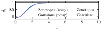
Figure 2: Evolution of the point-wise parameter estimate generated by the RLS algorithm developed in this paper. In each plot, the black line denotes the true value of the parameters.

The quadrotor is tasked with tracking the trajectory

$$q_{\mathrm{d}}(t)=\begin{bmatrix}4\sin(0.1\pi t)\\ 4\sin(0.1\pi t)\cos(0.1\pi t)\end{bmatrix},$$

which is accomplished using an adaptive control Lyapunov function (aCLF)-based controller [2, 5, 8] while avoiding a pair of circular obstacles in the workspace. The distance to each obstacle is expressed as

$$d_{i}(x)=\|q-q_{o,i}\|^{2}-r_{i}^{2},\quad i\in\{1,2\},$$

where $q_{o,i}\in\mathbb{R}^{2}$ is the obstacle’s center and $r_{i}\in\mathbb{R}_{>0}$ is its radius, which is extended to a relative degree one function using an approach similar to that of [28] to obtain the CBF:

$$h_{i}(x)=d_{i}(x)-\mu\min\{0,L_{f}d_{i}(x)\}L_{f}d_{i}(x),\quad i\in\{1,2\},$$

with $\mu\in\mathbb{R}_{>0}$. To enforce safety in the presence of uncertain parameters we leverage the robust and probabilistic approaches to safety using CBFs outlined in the previous section. We compare the performance of these two approaches to those that do not enforce safety (i.e., only attempt to track the desired trajectory) and those that robustly enforce safety (i.e., accounting for the worst-case uncertainty without attempting to reduce such uncertainty using data collected online).

The results of these simulations are provided in Fig. 1 - 3. Fig. 1 illustrates the trajectories of the quadrotor under each controller, Fig. 2 illustrates the evolution of the parameters produced by the RLS algorithm, and Fig. 3 illustrates the evolution of the zonotopes and Gaussian distribution resulting from the set-based estimation scheme. The orange curve in Fig. 1 represents the trajectory under the aCLF controller (from [8]) that only attempts to track the desired trajectory without accounting for safety. This controller achieves its trajectory tracking task but violates the safety requirement as the desired trajectory slightly overlaps with each obstacle. On the other extreme, the robust controller (green curve) – that enforces safety for all realizations of the parameters but does not perform online adaptation – achieves the safety requirement but exhibits poor tracking performance as the CBF is overly cautious and prohibits the quadrotor from navigating around the left obstacle. The controller for this simulation is obtained by filtering the aCLF controller through (23) using $\mathcal{Z}(\bar{\theta}_{0},\Sigma_{0})$. When combining this robust approach with the online RLS algorithm that continuously reduces the level of uncertainty, however, the quadrotor improves its tracking performance while guaranteeing safety, as illustrated by the blue and purple curves in Fig. 1. This improvement is facilitated by the convergence of both the point-wise and set-based estimates of the parameters as shown in Fig. 2 and Fig. 3. The point-wise estimates (which correspond to the center of the zonotope and mean of the Gaussian distribution used in the set-based estimates) of the parameters converge close to their true values after about 5 seconds in the presence of noise and converge exactly to their true values in the absence of noise as predicted by Theorem 2. Moreover, the uncertainty in these estimates decreases as such estimates improve. This is seen in Fig. 3 where the zonotopes shrink over time yet always contain the true parameters as guaranteed by Theorem 3, and the covariance of the Gaussian distribution decreases as the mean approaches the true values of the parameters.

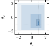
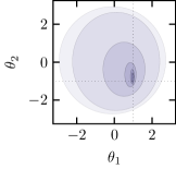
Figure 3: Evolution of the zonotopes (left) and Gaussian distributions with 95 % confidence ellipsoids (right) over the first four seconds of the simulations. The least opaque shape in each plot corresponds to the initial zonotope/Gaussian and darker shapes correspond to the estimates generated as time progresses. The intersection of the dotted lines represents the true value of the parameters.

VII Conclusions

In this paper, we presented a recursive least squares framework for online parameter estimation and uncertainty quantification in the context of adaptive safety-critical control. We demonstrated that such an approach allows for parameterizing the uncertainty using objects that are closed under affine transformation, which naturally led to uncertainty quantification of the parameter estimates using zonotopes and Gaussians. Such developments were motivated by their eventual integration with control barrier functions, which ultimately allowed for synthesizing controllers enforcing safety of nonlinear systems with parametric uncertainties. Future research will focus on extensions to systems with disturbances, measurement noise, and unmatched uncertainty.

References

- [1] P. A. Ioannou and J. Sun, Robust Adaptive Control. Dover, 2012.
- [2] M. Krstić, I. Kanellakopoulos, and P. Kokotović, Nonlinear and adaptive control design. John Wiley & Sons, 1995.
- [3] A. D. Ames, S. Coogan, M. Egerstedt, G. Notomista, K. Sreenath, and P. Tabuada, “Control barrier functions: theory and applications,” in Proc. Eur. Control Conf., pp. 3420–3431, 2019.
- [4] A. D. Ames, X. Xu, J. W. Grizzle, and P. Tabuada, “Control barrier function based quadratic programs for safety critical systems,” IEEE Trans. Autom. Control, vol. 62, no. 8, pp. 3861–3876, 2017.
- [5] A. J. Taylor and A. D. Ames, “Adaptive safety with control barrier functions,” in Proc. Amer. Control Conf., pp. 1399–1405, 2020.
- [6] B. T. Lopez, J. J. Slotine, and J. P. How, “Robust adaptive control barrier functions: An adaptive and data-driven approach to safety,” IEEE Contr. Syst. Lett., vol. 5, no. 3, pp. 1031–1036, 2021.
- [7] A. Isaly, O. S. Patil, R. G. Sanfelice, and W. E. Dixon, “Adaptive safety with multiple barrier functions using integral concurrent learning,” in Proc. Amer. Control Conf., pp. 3719 – 3724, 2021.
- [8] M. H. Cohen and C. Belta, “High order robust adaptive control barrier functions and exponentially stabilizing adaptive control lyapunov functions,” in Proc. Amer. Control Conf., pp. 2233–2238, 2022.
- [9] M. H. Cohen and C. Belta, “Modular adaptive safety-critical control,” arXiv preprint arXiv:2303.04241, 2023.
- [10] B. T. Lopez and J. J. Slotine, “Unmatched control barrier functions: Certainty equivalence adaptive safety,” arXiv preprint arXiv:2207.13873, 2022.
- [11] M. Black, E. Arabi, and D. Panagou, “A fixed-time stable adaptation law for safety-critical control under parametric uncertainty,” in Proc. Eur. Control Conf., pp. 1328–1333, 2021.
- [12] M. Black and D. Panagou, “Safe control design for unknown nonlinear systems with koopman-based fixed-time identification,” arXiv preprint arXiv:2212.00624, 2022.
- [13] M. H. Cohen, C. Belta, and R. Tron, “Robust control barrier functions for nonlinear control systems with uncertainty: A duality-based approach,” in Proc. Conf. Decis. Control, pp. 174–179, 2022.
- [14] G. Chowdhary, Concurrent learning for convergence in adaptive control without persistency of excitation. PhD thesis, Georgia Institute of Technology, Atlanta, GA, 2010.
- [15] G. Chowdhary and E. Johnson, “A singular value maximizing data recording algorithm for concurrent learning,” in Proc. Amer. Control Conf., pp. 3547–3552, 2011.
- [16] L. Brunke, S. Zhou, and A. P. Schoellig, “Barrier bayesian linear regression: Online learning of control barrier conditions for safety-critical control of uncertain systems,” in Proc. Conf. Learning for Dyn. and Control, pp. 881–892, 2022.
- [17] F. Castañeda, J. J. Choi, W. Jung, B. Zhang, C. J. Tomlin, and K. Sreenath, “Probabilistic safe online learning with control barrier functions,” arXiv preprint arXiv:2208.10733, 2022.
- [18] V. Dhiman, M. J. Khojasteh, M. Franceschetti, and N. Atanasov, “Control barriers in bayesian learning of system dynamics,” IEEE Trans. Autom. Control, vol. 68, no. 1, pp. 214–229, 2023.
- [19] R. Sinha, J. Harrison, S. M. Richards, and M. Pavone, “Adaptive robust model predictive control with matched and unmatched uncertainty,” in Proc. Amer. Control Conf., pp. 906–913, 2022.
- [20] B. T. Lopez, Adaptive robust model predictive control for nonlinear systems. PhD thesis, Massachusetts Institute of Technology, 2019.
- [21] J. F. Fisac, A. K. Akametalu, M. N. Zeilinger, S. Kaynama, J. Gillula, and C. J. Tomlin, “A general safety framework for learning-based control in uncertain robotic systems,” IEEE Trans. Autom. Control, vol. 64, no. 7, pp. 2737–2752, 2019.
- [22] A. Girard, “Reachability of uncertain linear systems using zonotopes,” in Proc. Int. Conf. Hybrid Syst. Comp. Control, pp. 291–305, 2005.
- [23] M. R. Deisenroth, A. A. Faisal, and C. S. Ong, Mathematics for Machine Learning. Cambridge University Press, 2020.
- [24] M. Althoff, G. Frehse, and A. Girard, “Set propagation techniques for reachability analysis,” Annu. Rev. Control Robot. Auton. Syst., vol. 4, pp. 369–395, 2021.
- [25] S. Sadraddini and R. Tedrake, “Linear encodings for polytope containment problems,” in Proc. Conf. Decis. Control, pp. 4367–4372, 2019.
- [26] R. Cheng, M. J. Khojasteh, A. D. Ames, and J. W. Burdick, “Safe multi-agent interaction through robust control barrier functions with learned uncertainties,” in Proc. Conf. Decis. Control, pp. 777–783, 2020.
- [27] N. M. T. Kokolakis and K. G. Vamvoudakis, “Safety-aware pursuit-evasion games in unknown environments using gaussian processes and finite-time convergent reinforcement learning,” IEEE Trans. Neural Net. Learning Syst., 2022.
- [28] J. Breeden and D. Panagou, “High relative degree control barrier functions under input constraints,” in Proc. Conf. Decis. Control, pp. 6119–6124, 2021.