InfluencerRank: Discovering Effective Influencers via Graph Convolutional Attentive Recurrent Neural Networks
Abstract
As influencers play considerable roles in social media marketing, companies increase the budget for influencer marketing. Hiring effective influencers is crucial in social influencer marketing, but it is challenging to find the right influencers among hundreds of millions of social media users. In this paper, we propose InfluencerRank that ranks influencers by their effectiveness based on their posting behaviors and social relations over time. To represent the posting behaviors and social relations, the graph convolutional neural networks are applied to model influencers with heterogeneous networks during different historical periods. By learning the network structure with the embedded node features, InfluencerRank can derive informative representations for influencers at each period. An attentive recurrent neural network finally distinguishes highly effective influencers from other influencers by capturing the knowledge of the dynamics of influencer representations over time. Extensive experiments have been conducted on an Instagram dataset that consists of 18,397 influencers with their 2,952,075 posts published within 12 months. The experimental results demonstrate that InfluencerRank outperforms existing baseline methods. An in-depth analysis further reveals that all of our proposed features and model components are beneficial to discover effective influencers.
Introduction
Influencers are known as individuals who influence a magnificent number of people on social media. This, in turn, has attracted great attention to marketers since influencers and their huge fan bases can be considered as marketing channels and audiences, respectively (De Veirman, Cauberghe, and Hudders 2017; Evans et al. 2017). More recently, companies have started hiring influencers to advertise products for targeted audiences and expand brand awareness.
Due to the rapid growth of social media and influencer marketing, discovering effective influencers on social media has become increasingly important (Riquelme and González-Cantergiani 2016; Kang et al. 2018; Kim et al. 2020). For measuring user influence on social media, well-known metrics, such as the numbers of followers, retweets, and mentions, have been widely applied (Bakshy et al. 2011; Segev, Avigdor, and Avigdor 2018). In addition, information propagation (Romero et al. 2011; Silva et al. 2013; Kempe, Kleinberg, and Tardos 2003), social connections (Li, Lai, and Chen 2011), network centrality (Chen and Teng 2017), transparency (Kim, Jiang, and Wang 2021), and multi-relational network (Ma, Liu, and Chi 2018) have been used to identify influencers on social media. Among the various measures, the effectiveness of influence (Liu et al. 2015), often measured by the engagement rate (De Veirman, Cauberghe, and Hudders 2017; Kim and Han 2020; Kim et al. 2021; Lou and Yuan 2019; Comcowich 2018), has been considered as crucial in identifying effective influencers especially in the marketing domain. The engagement rate can be calculated as the ratio of the average number of likes to the number of followers, which essentially shows how much audiences engage with the corresponding influencer.
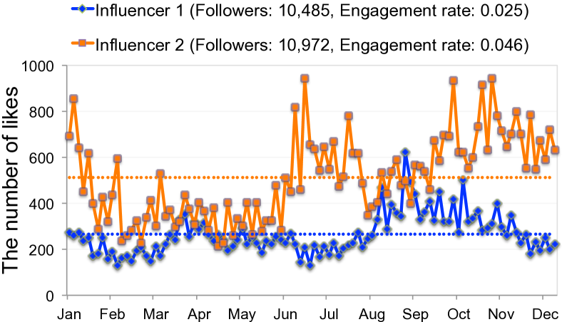
To discover the effective influencers (i.e., influencers with high engagement rates), previous work used posting behaviors of influencers or characteristics of their posts. For example, Romero et al. (2011), Liu et al. (2015), and Feng et al. (2018) utilized the social networks among influencers; Li, Lai, and Chen (2011) analyzed post contents to derive statistical features in identifying influencers. However, none of these studies jointly and comprehensively modeled posting behaviors, post characteristics, and social networking behaviors, which may result in a biased or partial representation of the effectiveness of influencer. For example, as shown in Figure 1, two influencers have similar numbers of followers hence they may be considered as having similar effectiveness, but their actual engagement rates are shown to be significantly different. Although some methods applied the PageRank algorithm on influencer-content graphs (Silva et al. 2013) and independently derived the features of influencers and posts (Liu et al. 2015), the PageRank algorithm can be biased to a certain type of nodes (Brezinski and Redivo-Zaglia 2006) when the relations between influencers and posts are ignored by independent features.
To address this issue, we propose to use a heterogeneous network to model the effectiveness of influencers with their posting behavior, social networking behavior, and post characteristics together. In addition, considering historical behavioral patterns can be further beneficial to discover effective influencers since posting behavior of an influencer can change dynamically over time. For instance, as shown in Figure 1, although an influencer does not receive many likes in the most recent time period, he/she may receive many number of likes in the future if he/she was used to get great attention in the past. Moreover, analyzing time-varying behavior patterns can provide more evidence on the robustness of an influencer. For example, the unstable performance (or effectiveness) of an influencer over time may not be desirable even if he/she satisfies the performance in the most recent time period. Hence, taking such time-varying behavior patterns into account for discovering effective influencers is essential. However, most of the prior studies only focused on the most recent information without considering the historical patterns of influencers.
In this paper, we propose InfluencerRank, a learning framework, that discovers effective influencers in social media by learning historical behavioral patterns of influencers. For comprehensively representing the effectiveness of an influencer, we build a heterogeneous information network that consists of influencers, hashtags, user tags, and image objects used by influencers for each historical time period (Yang et al. 2020; Zhang et al. 2019). To learn the complex posting behaviors, social networking, and post characteristics of each influencer, we apply graph convolutional networks (GCNs) (Kipf and Welling 2016) with well-designed influencer features, thereby deriving the influencer representation at a certain period. Based on the influencer representations over different historical time periods, the attentive recurrent neural network is proposed to learn the sequential and temporal behaviors to derive an ultimate representation. Finally, a learning-to-rank framework ranks a list of influencers to discover the ones who are more effective than others.
We summarize our contributions as follows:
-
•
To the best of our knowledge, this is the first attempt to rank influencers with their effectiveness by learning their historical behavioral patterns in social media marketing. We believe our model can be used for influencer recommendations that help companies to recruit a set of effective influencers to boost the advertising effect in social media.
-
•
The InfluencerRank uses the graph convolutional networks over general social media features to learn the posting behavior of the influencers as well as the characteristics of their posts, thus it can be applied to any social media to discover effective influencers. Besides, recurrent neural networks are also applied to model sequential and historical behaviors of influencers over time. We conduct experiments on a real-world dataset collected from Instagram (Kim et al. 2020), one of the most popular social media for influencer marketing (Nanji 2017). The results demonstrate that InfluencerRank outperforms other existing methods for identifying effective influencers.
-
•
Our analysis further reveals that the image object nodes have more impact on discovering effective influencers than other types of nodes since they can densely connect influencers thereby removing noises in the network. We also find that user reactions and visual perception of images are important features to find effective influencers.
-
•
We evaluate our proposed model over groups of influencers with different numbers of followers, and highlight that InfluencerRank shows effective and robust ranking performances across various groups of influencers.
Related Work
Influence Prediction in Social Networks
To find influencers in social networks, most studies rely on social media features to measure the influence. For example, the number of followers, posts, reposts, and mentions are well-known metrics to measure the influence of a user (Bakshy et al. 2011; Subbian and Melville 2011). Based on the measures, Bakshy et al. (2011) use the regression tree model and Subbian and Melville (2011) aggregate rank results to rank influencers, respectively. Romero et al. (2011) propose the passivity of nodes to measure how likely the information is propagated in the social networks, and then apply the PageRank to rank the users. Liu et al. (2015) consider the time domain over the user trust network in the proposed framework to classify influencers into one of three categories, emerging influencers, holding influencers, and vanishing influencers. In addition to social network features, some studies propose to use machine learning with statistical features. Li, Lai, and Chen (2011) extract network-based, content-based, and user activeness-based statistical features, e.g., the number of followers, and length of posts, to predict the influence of users. Segev, Avigdor, and Avigdor (2018) use simple statistics of posts and users, e.g., the number of likes, comments, followers, and posts, to measure the user influence using a regression model. Some previous works, on the other hand, exploit graphical information. Zhang et al. (2015) exploit the social influence locality to predict retweet behaviors. Qiu et al. (2018) utilize mini-batches of sub-graphs and apply the attention mechanism to predict the influence of users on social networks. Chen et al. (2019) propose recurrent convolutional networks to consider temporal effect on information cascade prediction. However, most previous works fail to consider temporal dynamics in the social relationships and characteristics of users.
Graph Convolutional Recurrent Networks
Graph convolutional networks (GCNs) (Kipf and Welling 2016) are the neural network architecture for graph-structured data. GCNs deploy spectral convolutional structures with localized first-order approximations so that the knowledge of both node features and graph structures can be leveraged. However, while real-world data that can be modeled as graphs dynamically changes over time, temporal information cannot be easily captured from GCNs. To learn the temporal dynamics of structural graphs, previous studies suggest to combine GCN and recurrent neural networks (RNNs). Seo et al. (2018) propose the models that (i) stack up graphs to make RNN inputs and (ii) consider convolutions in RNNs, which can learn a sequence of structural information. They find that each model outperforms the other models depending on applications such as video prediction and natural language modeling. Pareja et al. (2020) propose another approach to capture graph dynamics. Instead of using a sequence of graph embedding as inputs of RNN, they first use RNN to acquire the knowledge of network parameter dynamics. This approach can benefit in a case where a node dynamically appears and disappears. This paper proposes to apply attentive recurrent networks over the temporal node representations by taking a heterogeneous network that consists of influencers, image objects, hashtags, and user tags over time. Our model can effectively learn temporal graph representations by estimating the importance of hidden states for certain time periods.
Problem Statement
In this section, we formally define the effectiveness metric of an influencer and then formulate the problem of discovering effective influencers.
Definition 1.
Engagement rate is a widely-used metric in influencer marketing that shows how much audiences actively engage with an influencer (De Veirman, Cauberghe, and Hudders 2017; Kim et al. 2021; Kim and Han 2020; Lou and Yuan 2019; Comcowich 2018). Given an influencer , the engagement rate of the influencer at time is calculated as follows:
| (1) |
where is the number of followers who follow the influencer and is the average number of likes on content posted by the influencer at timestamp .
Based on the definition of influencer effectiveness, we introduce the influencer ranking problem. Let be the set of influencers. For each timestamp , we suppose that an influencer has published a set of posts . Given the set of influencers and their posts published until time , , the goal of this work is to discover influencers with high engagement rates at time by ranking all influencers so that is greater than if the influencer is ranked higher than the influencer .
Influencer Ranking Model Framework
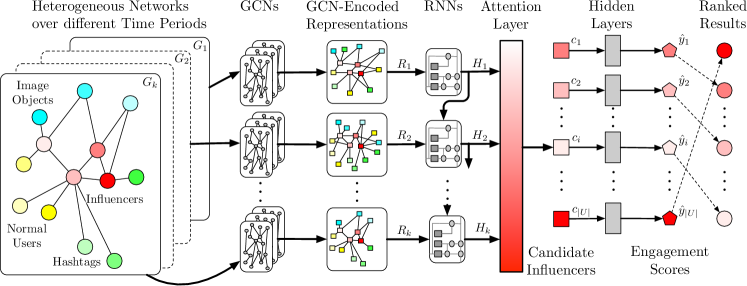
In this section, we propose InfluencerRank that learns the temporal dynamics of the engagement rates of influencers to automatically discover highly effective influencers. Figure 2 shows the overall framework of the proposed InfluencerRank. The framework takes a series of influencer social networks as input, where each network is composed of influencers and different entities, including but not limited to image objects, hashtags, and other users in social media. The graph convolutional networks (GCNs) are then applied to the input social networks to derive appropriate node representations that capture social relationships and posting characteristics of influencers at a certain time. The GCN-encoded representations across different times are then fed into a recurrent neural network to learn from the sequence of the node representations. The attention mechanism is then applied to the whole sequence of representations to finally derive the effectiveness scores of candidate influencers and rank them for discovering effective influencers.
| Notation | Description |
|---|---|
| the engagement rate of an influencer at time . | |
| the average number of engagements on contents posted by the influencer at time . | |
| the number of followers for an influencer at time . | |
| the set of influencers. | |
| the posts published by the influencer at time . | |
| the heterogeneous network for time with the node features and the adjacency matrix . | |
| Normalized adjacency matrix transformed from . | |
| the number of dimensions for embedded node features. | |
| the diagonal degree matrix of . | |
| the number of hidden dimensions in GCNs. | |
| the outputs of the -th GCN layer. | |
| the weight matrix between and . | |
| the GCN-encoded representation for time . | |
| the hidden states in the RNN for time . | |
| the list of hidden states in the RNN over time. | |
| the importance weight for . | |
| the fully-connected layer for deriving . | |
| the normalized importance weight for . | |
| the final representation of the influencer . | |
| the predicted engagement score for the influencer . | |
| the fully-connected layers for inferring . |
Heterogeneous Information Networks
To represent the dynamics of the engagement rates on a sequence of time, we build heterogeneous networks based on the influencers and other relevant entities. Hence, can further characterize the relationships of influencers and their posting behaviors at time .
Heterogeneous Nodes and Embedded Features
We build a heterogeneous network for time with four different types of nodes, including influencers, hashtags, image objects, and other users in social media. Given an influencer , we extract all of the hashtags and mentioned users (i.e., user tags) from posts , where and indicate the number of extracted hashtags and mentioned users, respectively. Note that the mentioned users can be either influencers, brands, or other normal users. In addition, the categories of objects shown in the posted images are also considered as nodes. Since each type of node has unique features, we denote the node features of influencers, mentioned users, hashtags, and object categories in images as , , , and , respectively. We then represent embedded features of each node as where is the total number of all four types of nodes and is the number of embedded node features.
Edge Construction and Adjacency Matrix
The edges in the heterogeneous network indicate the interactions between entities behind nodes. For example, if an influencer mentioned the hashtag #makeup and posted an image of cosmetic products, the influencer node will be connected to the node of the #makeup hashtag and the node of the cosmetic image object. Given a timestamp , we make a sparse adjacency matrix , where indicates a connection between the -th and -th nodes.
Finally, a set of heterogeneous networks with the sets of node features and adjacency matrices can be constructed as follows:
where indicates both the node embedded features and the heterogeneous network structure at time .
Graph Convolutional Networks
For the heterogeneous network of each time , our proposed InfluencerRank applies Graph Convolutional Networks (GCNs) (Kipf and Welling 2016) to generate node representations over time. GCNs first generate a normalized adjacency matrix by transforming the adjacency matrix with the diagonal degree matrix as GCNs then stack multiple GCN layers where each layer takes outputs of the previous layer and performs nonlinear transformation to propagate information through different layers. The -th layer in GCNs then outputs as follows:
where is the number of hidden dimensions in GCNs, is the outputs of the previous layer, is a matrix of trainable weights, and is a nonlinear activation function. We use for as the input of the first GCN layer. The final output of the GCNs at time can be represented as follows:
where is the number of layers in GCNs.
Finally, we can obtain a sequence of GCN-encoded node representations, , to implicitly represent the knowledge about influencers over time.
Attentive Recurrent Neural Networks
Learning Graph Dynamics
Based on the sequence of GCN-encoded node representations, , InfluencerRank applies Recurrent Neural Networks (RNNs) to the model framework. More specifically, we employ Gated Recurrent Units (GRUs) (Cho et al. 2014), which use update gate and reset gate inside the unit to carry information flow over many time periods, to capture long-term temporal dependencies from the heterogeneous networks. Each GRU takes hidden states from the previous unit and the GCN representations as input and then outputs hidden states of the current time. More formally, the hidden states at time , is computed as follows:
| (2) |
where is an update gate at time and is the candidate state at time . The candidate state is updated as follows:
| (3) |
where is an reset gate at time , is an element-wise multiplication, and is the GCN representations at time . Finally, InfluencerRank obtains the whole states of GRUs as follows:
Attention over Time
To acquire the final influencer representations, InfluencerRank applies the attention mechanism (Bahdanau, Cho, and Bengio 2014) to the whole state embeddings derived from GRUs . The attention mechanism allows InfluencerRank to learn the dynamics of the engagement rates by taking into account the importance of time periods.
For each timestep , InfluencerRank estimates the importance weight of the corresponding state embedding by applying a projection as:
| (4) |
where is a fully-connected layer; is the activation function. We then compute the weights of each timestep by using a softmax function as:
| (5) |
Finally, InfluencerRank derives the ultimate representation of candidate influencers by using the weighted sum as follows:
| (6) |
Engagement Score Estimation
For an influencer , InfluencerRank takes the corresponding ultimate representation as the input and then predicts an engagement score that is proportional to the engagement rate as follows:
| (7) |
where a non-linear transformation is carried out in a fully-connected layer with the ReLU activation function and the engagement rate is estimated in another fully-connected layer .
List-wise Ranking and Optimization
InfluencerRank treats the task as a ranking problem and optimizes the ranking performance with a list-wise learning-to-rank framework (Xia et al. 2008). Suppose is the set of features for influencers to be ranked; is the space of all possible rankings. During training, we sample labeled influencers from the whole training space as an i.i.d. candidate ranked list where is the unknown target joint probability distribution of and . Therefore, the corresponding loss can be considered as:
| (8) |
where is the 0-1 loss between and the rank in ; denotes the ground-truth ranking such that
| (9) |
Node Features
In this subsection, we describe node features in the heterogeneous network. To understand the relationship between the engagement rate of an influencer and the characteristics of the corresponding influencer, we introduce six types of node features, including node type, profile, image, text, posting, and reaction features.Note that most of the features are only applicable for influencer nodes while the remaining nodes (e.g., hashtags, image objects) hold zeros for the inapplicable features. For the feature engineering, we deploy the average, median, minimum, and maximum values for the features that need to be aggregated with statistics.
Here, we briefly introduce the six categories of features used in this paper as follows.
-
•
Node type features. The one-hot coded feature that indicates one of the four node types, including influencers, other users, hashtags, and image objects.
-
•
Profile features. For each influencer node, we exploit the numbers of followers, followees, and posts which are the most commonly used metrics to measure user influence in social networks (Riquelme and González-Cantergiani 2016). Additionally, we consider a category of influencers from eight influencer categories defined in the previous study (Kim et al. 2020).
-
•
Image features. The previous study (Gelli et al. 2015) showed that the characteristics of images on social media posts affect its popularity. In addition to the image objects which are considered as nodes in the heterogeneous network, we add the attributes of visual perception of the images to understand how influencers create images. We compute the brightness, colorfulness (Hasler and Suesstrunk 2003), and color temperature of the posted images based on their RGB values.
-
•
Text features. To understand how textual usage of influencers affects the engagement rate, we retrieve various text features. More specifically, we use the numbers of hashtags, user tags, and emojis that are widely used functions on social media, and the length of captions which can represent how much detailed information is in the caption (Hessel, Lee, and Mimno 2017). Moreover, we also calculate the sentiment scores of captions to learn how positive or negative emotions are carried through the captions by using VADER (Gilbert and Hutto 2014).
-
•
Posting features. The features in this category can provide information about how influencers use social media from various aspects. We first exploit the portion of the number of posts in one of the ten post categories (Kim et al. 2020) to the total number of posts to understand the posting behavior of influencers. In addition to the post category rate feature, we also examine the portion of the number of advertising posts to the total posts published by an influencer; posting too many paid advertisements can show negative impacts on the popularity (Evans et al. 2017; Yang, Kim, and Sun 2019). We also consider the feedback rate and posting interval, which are the measures of the interaction with their followers and activeness, respectively. The feedback rate is calculated as the ratio of the number of posts that contain the influencers’ responses to the user comments to the number of total posts. The posting interval is the average time gap between posts that are in chronological order.
-
•
Reaction features. We use the user comments to generate the user reaction feature. Specifically, we compute the sentiment scores of comments that are written by audiences of the influencers’ posts. Note that we do not consider the number of likes and comments as node features since it can directly imply the engagement rates of influencers.
Experiments
In this section, we conduct experiments to evaluate the performance of InfluencerRank compared with other baseline methods. We also analyze the experimental results to understand the importance of each feature to find influencers with high engagement rates.
Experimental Dataset
Dataset Construction
To evaluate the proposed InfluencerRank, we use the Instagram influencer dataset (Kim et al. 2020). The dataset includes profiles of influencers, and their posts, including both images and all meta-data. We only keep the posts that were published in the range of January 1st, 2017 and December 31st, 2017, to build temporal influencer networks. As a result, the dataset consists of 18,397 influencers and 2,952,075 posts. For the experiments, we split the dataset into the training dataset, which contains posts from January to November, and the testing dataset that contains posts published in December.
Heterogeneous Network Construction
To build the temporal heterogeneous networks, we first divide the whole dataset into 12 subsets by one-month intervals. Note that we conduct experiments to analyze ranking performances across different temporal window sizes, thereby having the proper time intervals. We then extract all hashtags and user tags from the post captions and detect objects from the images. As a consequence, 1,151,082 unique hashtag nodes, 532,468 other user nodes, and 1,000 image object nodes are found across the networks and connected to the corresponding influencer nodes. To further reduce noises in the dataset, we remove every auxiliary node (i.e., hashtags, other users, and image objects) with only a single edge while edges with normalized frequencies less than 0.01 are also discarded. After the pruning process, 18,397 influencers, 20,744 other users, 67,695 hashtags, and 996 image objects are in the networks (i.e., 107,832 nodes), and a total of 15,090,225 edges remain across the networks.
Experimental Settings
Evaluation Metrics
Based on the definition, we first compute the engagement rates for all influencers in across all timesteps as the ground truths. Note that the average engagement rate is 0.038 and the median engagement rate is 0.029. We utilize two metrics to evaluate the performance of ranking influencers.
-
•
Normalized Discounted Cumulative Gain (NDCG) (Järvelin and Kekäläinen 2017): First, we divide all of the influencers into six groups with different thresholds on the engagement rates and relevance levels from 0 to 5. Table 2 further shows the statistics of influencers in the dataset across different relevance levels and criteria for the engagement rates. We then treat the relevance levels as ground truths to evaluate the ranking performance with the metric of NDCG.
-
•
Rank-Biased Precision (RBP) (Moffat and Zobel 2008): To avoid losing valuable information while converting the engagement rates to the six relevance levels, we directly use the engagement rates with the metric of RBP. We set the probability as 0.95 to measure rank quality.
| Relevance | Engagement rate | Number of Influencers |
|---|---|---|
| 5 | 1,274 (6.92%) | |
| 4 | 1,678 (9.12%) | |
| 3 | 2,321 (12.62%) | |
| 2 | 4,509 (24.51%) | |
| 1 | 6,882 (37.41%) | |
| 0 | 1,734 (9.42%) |
Implementation Details
For the hyperparameter tuning, we use a validation set which contains posts published by the 18,397 influencers in January 2018. Since our model is optimized with the validation set, we can avoid potential information leakage from the testing set. In order to fine-tune the model, we train the proposed neural network with different sets of parameters, including the number of GCN layers and its dimensions, the size of influencer list for ranking, batch size, learning rate, and dropout probability. After tuning the model, we set the numbers of dimensions of the graph embeddings and GCN features as 128, and the number of GCN layers as 2. Each batch contains 1,024 lists of influencers, and each list includes 10 randomly selected influencers for list-wise learning. The learning rate and the dropout probability are set as 0.001 and 0.5, respectively.
| Method | RBP | NDCG@K | Time | ||||
| 1 | 10 | 50 | 100 | 200 | (sec) | ||
| UP | 0.025 | 0.800 | 0.436 | 0.413 | 0.406 | 0.368 | 347 |
| PP | 0.028 | 1.000 | 0.519 | 0.465 | 0.442 | 0.425 | 295 |
| UA | 0.024 | 0.800 | 0.518 | 0.494 | 0.438 | 0.436 | 330 |
| LN | 0.026 | 1.000 | 0.610 | 0.511 | 0.465 | 0.441 | 481 |
| LM | 0.031 | 1.000 | 0.648 | 0.546 | 0.493 | 0.477 | 563 |
| GCRN | 0.028 | 1.000 | 0.629 | 0.557 | 0.513 | 0.467 | 612 |
| DeepInf | 0.031 | 1.000 | 0.697 | 0.567 | 0.549 | 0.512 | 525 |
| CasCN | 0.033 | 1.000 | 0.751 | 0.645 | 0.572 | 0.543 | 1109 |
| EGCN | 0.038 | 1.000 | 0.812 | 0.679 | 0.616 | 0.577 | 1483 |
| InfluencerRank | 0.043 | 1.000 | 0.864 | 0.720 | 0.661 | 0.614 | 648 |
Baseline Methods
We compare the performance of InfluencerRank with nine baseline methods in three different categories, including User, Ranking, and Graph.
-
•
User baselines: The baseline methods in this category exploit information on social media to measure the popularity of users with certain features. Since user popularity is often to be considered as an important factor in influencer hiring (De Veirman, Cauberghe, and Hudders 2017; Lou and Yuan 2019; Casaló, Flavián, and Ibáñez-Sánchez 2018), we develop three baseline methods including user popularity (UP) (Bakshy et al. 2011), post popularity (PP) (Mazloom et al. 2016), user activity (UA) (Li, Lai, and Chen 2011).
- •
-
•
Model baselines: The baseline methods in this category implement graph neural networks (GNNs) based learning models. Note that the applied features of InfluencerRank and graph baselines are identical so that we can fairly evaluate the model novelty and capability for the ranking task. We develop GCRN (Seo et al. 2018), DeepInf (Qiu et al. 2018), CasCN (Chen et al. 2019), and EGCN (Pareja et al. 2020).
Experimental Results
Table 3 shows RBP, NDCG scores, and training time of InfluencerRank and the nine baseline methods for discovering influencers with high engagement rates. All of the three methods in the user baselines, which exploit the social media features, obtain low ranking results. This suggests that only considering social media features is insufficient to discover effective influencers. The ranking baseline methods, on the other hand, show better ranking performance compared to the user baseline methods since they use our proposed features. It demonstrates that our proposed features are very useful to capture the characteristics of influencers, thereby discovering effective influencers. Next, most of the graph baseline methods outperform the user baselines and ranking baselines. More specifically, among the graph baseline methods, GCRN (Seo et al. 2018) shows limited ranking performance improvement since it only resorts to temporal-spatial structures of graphs without taking into account the node features. DeepInf (Qiu et al. 2018) demonstrates better ranking performance than GCRN by exploiting the graph convolutional networks that take advantage of the network structures of different entities while the features in different aspects provide sufficient knowledge to describe both influencers and other entities in the graph. Both CasCN (Chen et al. 2019) and EGCN (Pareja et al. 2020) further improve performance by applying recurrent neural networks to adjacency matrices of temporal graphs. This suggests that the learning dynamics of graph structures with node features over time is beneficial in discovering effective influencers.
Finally, our proposed approach, InfluencerRank, outperforms all of the baseline methods. This is because our model derives informative influencer representations over time by using the graph convolutional networks and the attentive neural network, and effectively learns the dynamics of influencer characteristics and engagement rates. The results also show that InfluencerRank is able to learn the latent influencer representations in a reasonable amount of training time compared to the other baseline methods. CasCN and EGCN, on the other hand, have significantly longer training time than InfluencerRank. This is probably because the proposed framework successfully learns the importance of hidden states in the RNNs by applying attention while other baseline methods combine RNNs with GCNs without taking the importance of each temporal graph into account.
Analysis and Discussions
In this section, we conduct six analyses to understand the importance of (i) the temporal window size, (ii) the temporal information, (iii) the model components, (iv) the type of RNNs, (v) the heterogeneous networks, and (vi) the input features. We then evaluate the performance of InfluencerRank on various sets of influencers which are grouped by the size of audiences.
Analysis on Temporal Window Size
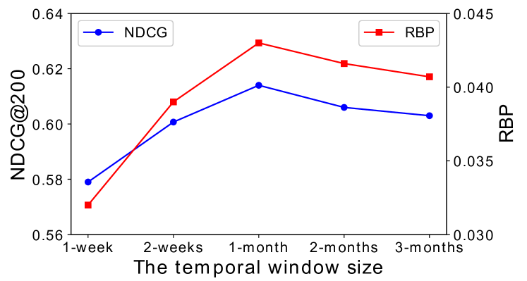
We first investigate the effect of different temporal window sizes for heterogeneous network construction. To that end, we split the training dataset which has posts in 11 months period into sub-datasets by five different temporal window sizes including 1 week, 2 weeks, 1 month, 2 months, and 3 months. Note that we use the same testing dataset across the five different window sizes for consistent performance comparison. The RBP and NDCG@200 scores of the InfluencerRank over the different temporal window sizes are shown in Figure 3. We find that the model trained with the networks divided by 1-month intervals shows the best ranking performance whereas the model trained with the 1-week temporal window has the lowest ranking scores. InfluencerRank loses 5.7% performance on NDCG when the model is trained with the 1-week window size compared to the model trained with the 1-month window size. This suggests that the heterogeneous networks of the models, which are trained with temporal window size shorter than 1-month, have insufficient information to learn the dynamics of engagement rates. We also observe that the ranking performance gradually decreases while we use the longer temporal window size. This implies that the model trained with a large window size fails to take into account the variance of engagements by using the average like counts of all posts in each sub-dataset. The analysis results also demonstrate that learning the temporal dynamics of the engagement rates is very important to find effective influencers.
Analysis on Temporal Information
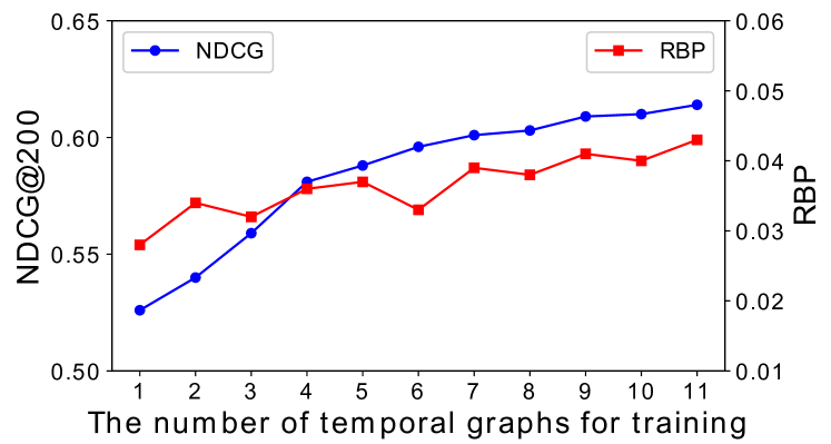
We next evaluate the ranking performance of the proposed model by using the different number of temporal input networks for training the model. Figure 4 shows RBP and NDCG@200 scores of the InfluencerRank over the number of temporal graphs. Note that the model uses the most recent temporal graphs. For example, a model trained with two temporal graphs learns two networks in October and November in our dataset. We observe that the performance significantly drops when InfluencerRank obtains insufficient historical information. InfluencerRank loses 15% performance on NDCG if the model uses only one graph compared to the model that considers all temporal graphs. The result confirms that only considering the most recent network degrades the performance since the engagement rates of influencers vary over time. We also find that as the number of temporal networks increases, the model has gradually less performance gain.
Analysis on Model Components
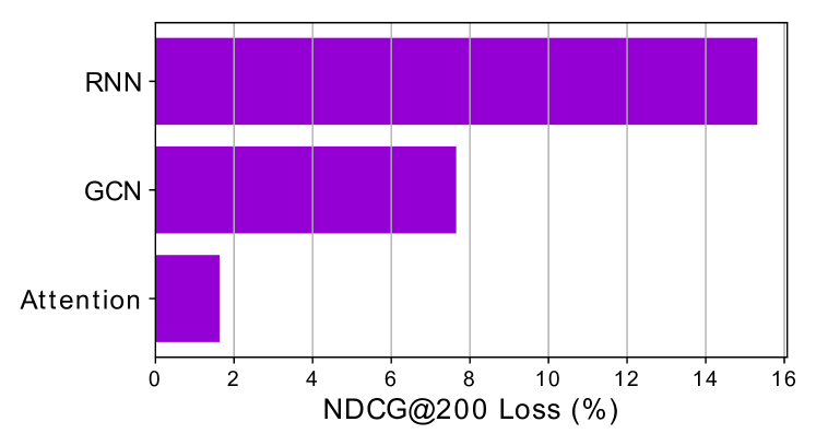
The proposed model consists of three major components, including the graph convolutional networks, the recurrent neural networks, and the attention network. We conduct an ablation study by excluding each component from the model framework to understand the importance of model components. Figure 5 shows the performance losses of NDCG@200 scores over the three model components. We find that the model which excludes the RNN component has significant performance loss compared to the full model. This suggests that disregarding to learn sequential temporal information leads to performance degradation since engagement rates of an influencer change over time. The model that discards the GCN component also shows large performance loss. This is because the model fails to learn structural information with embedded node features. This demonstrates that learning social relationships of influencers with other users, tags, and image objects plays an important role in discovering effective influencers. We observe that the attention component has relatively less impact on the performance than other model components whilst it still enhances the model by considering the importance of temporal graph embeddings.
Analysis on Recurrent Neural Networks
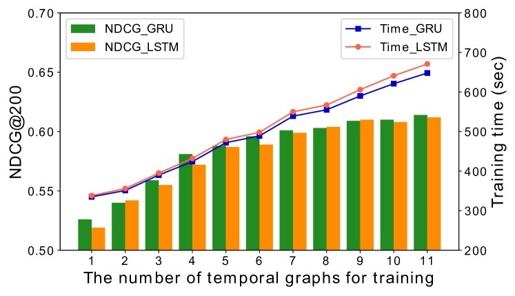
In the proposed InfluencerRank framework, we employ gated recurrent units (GRUs) (Cho et al. 2014) for the recurrent neural networks. However, the GRU can be replaced with a long short-term memory (LSTM) (Hochreiter and Schmidhuber 1997). To make a design decision which recurrent architecture to employ, we train InfluencerRank with GRU and LSTM. Figure 6 shows NDCG@200 scores and training times of InflurncerRank with two RNN architectures on different number of temporal graphs. We observe that no significant difference in the NDCG scores of models using GRU and LSTM, but the model with GRU tends to have slightly higher scores. The results also show that InfluencerRank with GRU has shorter training times than LSTM across the different number of temporal graphs. More specifically, the time difference gradually increases as the number of temporal graphs for training increases. Note that GRU is 1% faster than LSTM when the model only takes one temporal graph and 3.4% faster when the model uses 11 graphs for training. GRU shows better performance than LSTM in our task and that is probably because GRU has simpler network than LSTM and also benefits from the short input sequence length.
Analysis on Heterogeneous Networks
We study the importance of the proposed heterogeneous network to find effective influencers. To understand the importance of individual auxiliary node type, we train InfluencerRank with the network without the type of auxiliary node. Table 4 shows the RBP and the NDGC scores of InfluencerRank with different types of networks. The results show that the model trained with all types of nodes achieve higher RBP and NDCG scores than the other models that exclude a type of auxiliary nodes. This confirms that the graphical structure in InfluencerRank helps improve performance in finding effective influencers. We also observe that NDCG scores of the model without the image object nodes are lower than that of the model excluding hashtags and other user nodes. Note that excluding the image object nodes drops the performance of NDCG@200 by 4.1%, whereas excluding hashtag and other user nodes only drops the score by 2.8% and 1.9%. This is probably because each image object node can densely connect a large number of similar influencers together as it has a greater number of edges than a hashtag node and a user node.
| Node Type | RBP | NDCG@K | ||||
|---|---|---|---|---|---|---|
| 1 | 10 | 50 | 100 | 200 | ||
| All nodes | 0.043 | 1.000 | 0.864 | 0.720 | 0.661 | 0.614 |
| , , | 0.039 | 1.000 | 0.848 | 0.704 | 0.648 | 0.589 |
| , , | 0.040 | 1.000 | 0.863 | 0.716 | 0.654 | 0.602 |
| , , | 0.037 | 1.000 | 0.861 | 0.708 | 0.657 | 0.597 |
Analysis on Node Features
The benefit of using GCNs comes from considering network structure information with node features. To understand the importance of node features, we first evaluate the performance of the model that excludes all node categories. The model without the whole node features significantly drops the ranking quality; the loss of NDGC@200 of the model without node features is 21.99%.
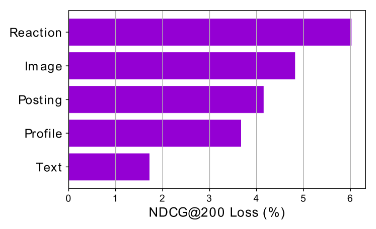
We then investigate the performance of InfluencerRank with variant sets of node features to study the importance of each category of the node features.Figure 7 shows the performance loss of NDCG scores of the models trained with the node features excluding one particular node category against the full model as the leave-one-out analysis. The results reveal that the reaction feature category, which contains the sentiment scores of user comments on the posts, is more important than other categories to identify effective influencers. This indicates that the audience may show distinct reactions to influencers with high engagement rates. The image category, which includes the visual perception of images (e.g., brightness, colorfulness), also has higher loss values than other node feature categories. This suggests that influencers with high engagement rates may have different visual characteristics from other influencers. On the other hand, the text category, including the number of hashtags, user tags, emojis in a caption, and the sentiment scores of the caption, have the least impact to discover effective influencers. Although the statistical features to represent textual characteristics of influencers’ posts have less impact than other features, InfluencerRank can improve the ranking performance by taking hashtags and user tags into account to the network structure.
Influencer Follower Size
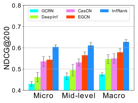
In the influencer marketing industry, influencers are often divided into subgroups by the number of followers since it directly refers to the size of potential customers and hiring cost (De Veirman, Cauberghe, and Hudders 2017). For example, companies with a sufficient marketing budget can hire influencers who are followed by millions of people while small retailers may collaborate with influencers with a small number of followers. Therefore, we evaluate the performance of InfluencerRank over groups of influencers with different sizes of followers. Although there are no standard criteria to classify influencers based on the number of followers, we utilize the following thresholds which are the generally accepted numbers to divide the influencers into three groups111http://www.mattr.co/pros-cons-micro-macro-mid-level-influencers/. Influencers who are followed by less than 20,000 followers are classified as the Micro influencers. The Mid-level influencers have followers between 20,000 and 100,000, and Macro influencers have more than 100,000 followers. In our dataset, around 30% of influencers are the micro-influencers, 45% of them are the mid-level influencers, and the remaining 25% influencers are the macro-influencers. To evaluate the performance under the same conditions, we randomly select multiple sets of 1,000 influencers from each category and run the experiment 10 times.
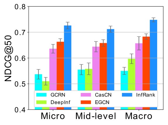
Figure 8 shows the average NDCG scores of InfluencerRank and four baseline methods, including GCRN (Seo et al. 2018), DeepInf (Qiu et al. 2018), CasCN (Chen et al. 2019), and EGCN (Pareja et al. 2020) over the micro, mid-level, and macro-influencers. The results show that the proposed model has robust performance to discover effective influencers in the groups of all ranges of followers compared to the baseline methods. More specifically, DeepInf (Qiu et al. 2018) fails to discover effective micro-influencers. This is probably because DeepInf disregards the temporal information which is critical to find micro-influencers who have relatively large variance on their features and engagement rates over time compared to macro-influencers who are matured. On the other hand, our proposed model can accurately find highly effective micro-influencers since their unique features are captured by sequential learning of temporal information.
Conclusion
In this paper, we propose a ranking model to discover influencers with high engagement rates by learning temporal dynamics of their posting behaviors. To represent the characteristics of influencers and their posting behaviors at each time period, we build a heterogeneous network that consists of influencers and social media elements as nodes, such as hashtags, user tags, and image objects. Moreover, each node can be associated with context features in six categories, including node type, profile, image, text, posting, and reaction features. Based on the GCN-encoded representations of influencers at each timestamp, our proposed model applies attentive RNNs to model historical behaviors of influencers, thereby accurately ranking influencers by their engagement rate scores. The results of the extensive experiments show that InfluencerRank outperforms existing baseline methods.
Broader Impact and Ethical Considerations
The utility of our proposed framework is expected to significantly increase given a decision of Instagram, one of the most popular influencer marketing platform, that considers to hide the number of likes on each post (Instagram 2021; Loren 2019) to help mental health issues of social media users (Royal Society for Public Health 2017). Unlike prior work, the number of likes is not used in discovering influencers in InfluencerRank, hence our proposed model can be particularly used by brands with relatively small business sizes, who may be suffering from the heavy expense of discovering effective influencers among millions of candidates (Instagram 2017) in a situation where the number of likes is hidden from other users. Additionally, our model is also capable of adopting additional node features and node types in the network for further improvements. As a result, we believe our model can be widely exploited in finding highly effective influencers for businesses from small retailers to global brands.
References
- Bahdanau, Cho, and Bengio (2014) Bahdanau, D.; Cho, K.; and Bengio, Y. 2014. Neural machine translation by jointly learning to align and translate. arXiv preprint arXiv:1409.0473.
- Bakshy et al. (2011) Bakshy, E.; Hofman, J. M.; Mason, W. A.; and Watts, D. J. 2011. Everyone’s an influencer: quantifying influence on twitter. In Proceedings of the fourth ACM international conference on Web search and data mining, 65–74.
- Brezinski and Redivo-Zaglia (2006) Brezinski, C.; and Redivo-Zaglia, M. 2006. The PageRank vector: properties, computation, approximation, and acceleration. SIAM Journal on Matrix Analysis and Applications, 28(2): 551–575.
- Burges, Ragno, and Le (2007) Burges, C. J.; Ragno, R.; and Le, Q. V. 2007. Learning to rank with nonsmooth cost functions. In Advances in neural information processing systems, 193–200.
- Cao et al. (2007) Cao, Z.; Qin, T.; Liu, T.-Y.; Tsai, M.-F.; and Li, H. 2007. Learning to rank: from pairwise approach to listwise approach. In Proceedings of the 24th international conference on Machine learning, 129–136.
- Casaló, Flavián, and Ibáñez-Sánchez (2018) Casaló, L. V.; Flavián, C.; and Ibáñez-Sánchez, S. 2018. Influencers on Instagram: Antecedents and consequences of opinion leadership. Journal of Business Research.
- Chen and Teng (2017) Chen, W.; and Teng, S.-H. 2017. Interplay between social influence and network centrality: a comparative study on shapley centrality and single-node-influence centrality. In Proceedings of the 26th international conference on world wide web, 967–976.
- Chen et al. (2019) Chen, X.; Zhou, F.; Zhang, K.; Trajcevski, G.; Zhong, T.; and Zhang, F. 2019. Information diffusion prediction via recurrent cascades convolution. In 2019 IEEE 35th International Conference on Data Engineering (ICDE), 770–781. IEEE.
- Cho et al. (2014) Cho, K.; Van Merriënboer, B.; Gulcehre, C.; Bahdanau, D.; Bougares, F.; Schwenk, H.; and Bengio, Y. 2014. Learning phrase representations using RNN encoder-decoder for statistical machine translation. arXiv preprint arXiv:1406.1078.
- Comcowich (2018) Comcowich, W. 2018. Macro-Engagement of Micro-influencers Yields Marketing Dividends. GleanInfo.
- De Veirman, Cauberghe, and Hudders (2017) De Veirman, M.; Cauberghe, V.; and Hudders, L. 2017. Marketing through Instagram influencers: the impact of number of followers and product divergence on brand attitude. International Journal of Advertising, 36(5): 798–828.
- Evans et al. (2017) Evans, N. J.; Phua, J.; Lim, J.; and Jun, H. 2017. Disclosing Instagram influencer advertising: The effects of disclosure language on advertising recognition, attitudes, and behavioral intent. Journal of Interactive Advertising, 17(2): 138–149.
- Feng et al. (2018) Feng, S.; Cong, G.; Khan, A.; Li, X.; Liu, Y.; and Chee, Y. M. 2018. Inf2vec: Latent representation model for social influence embedding. In 2018 IEEE 34th International Conference on Data Engineering (ICDE), 941–952. IEEE.
- Gelli et al. (2015) Gelli, F.; Uricchio, T.; Bertini, M.; Del Bimbo, A.; and Chang, S.-F. 2015. Image popularity prediction in social media using sentiment and context features. In Proceedings of the 23rd ACM international conference on Multimedia, 907–910.
- Gilbert and Hutto (2014) Gilbert, C.; and Hutto, E. 2014. Vader: A parsimonious rule-based model for sentiment analysis of social media text. In Eighth International Conference on Weblogs and Social Media (ICWSM-14), volume 81, 82.
- Hasler and Suesstrunk (2003) Hasler, D.; and Suesstrunk, S. E. 2003. Measuring colorfulness in natural images. In Human vision and electronic imaging VIII, volume 5007, 87–95. International Society for Optics and Photonics.
- Hessel, Lee, and Mimno (2017) Hessel, J.; Lee, L.; and Mimno, D. 2017. Cats and captions vs. creators and the clock: Comparing multimodal content to context in predicting relative popularity. In Proceedings of the 26th International Conference on World Wide Web, 927–936.
- Hochreiter and Schmidhuber (1997) Hochreiter, S.; and Schmidhuber, J. 1997. Long short-term memory. Neural computation, 9(8): 1735–1780.
- Instagram (2017) Instagram. 2017. 2M Monthly Advertisers on Instagram. Accessed: 2017-09-25.
- Instagram (2021) Instagram. 2021. Giving People More Control on Instagram and Facebook. Accessed: 2021-05-26.
- Järvelin and Kekäläinen (2017) Järvelin, K.; and Kekäläinen, J. 2017. IR evaluation methods for retrieving highly relevant documents. In ACM SIGIR Forum, volume 51, 243–250. ACM New York, NY, USA.
- Kang et al. (2018) Kang, J.; Choi, D.; Park, E.; and Han, J. 2018. Understanding Influential Comments in Online Conversations. In Companion of the 2018 ACM Conference on Computer Supported Cooperative Work and Social Computing, 197–200.
- Kempe, Kleinberg, and Tardos (2003) Kempe, D.; Kleinberg, J.; and Tardos, É. 2003. Maximizing the spread of influence through a social network. In Proceedings of the ninth ACM SIGKDD international conference on Knowledge discovery and data mining, 137–146.
- Kim et al. (2021) Kim, S.; Chen, X.; Jiang, J.-Y.; Han, J.; and Wang, W. 2021. Evaluating Audience Loyalty and Authenticity in Influencer Marketing via Multi-task Multi-relational Learning. In ICWSM, 278–289.
- Kim and Han (2020) Kim, S.; and Han, J. 2020. Detecting engagement bots on social influencer marketing. In International Conference on Social Informatics, 124–136. Springer.
- Kim et al. (2020) Kim, S.; Jiang, J.-Y.; Nakada, M.; Han, J.; and Wang, W. 2020. Multimodal Post Attentive Profiling for Influencer Marketing. In Proceedings of The Web Conference 2020, 2878–2884.
- Kim, Jiang, and Wang (2021) Kim, S.; Jiang, J.-Y.; and Wang, W. 2021. Discovering undisclosed paid partnership on social media via aspect-attentive sponsored post learning. In Proceedings of the 14th ACM International Conference on Web Search and Data Mining, 319–327.
- Kipf and Welling (2016) Kipf, T. N.; and Welling, M. 2016. Semi-supervised classification with graph convolutional networks. arXiv preprint arXiv:1609.02907.
- Li, Lai, and Chen (2011) Li, Y.-M.; Lai, C.-Y.; and Chen, C.-W. 2011. Discovering influencers for marketing in the blogosphere. Information Sciences, 181(23): 5143–5157.
- Liu et al. (2015) Liu, S.; Jiang, C.; Lin, Z.; Ding, Y.; Duan, R.; and Xu, Z. 2015. Identifying effective influencers based on trust for electronic word-of-mouth marketing: A domain-aware approach. Information sciences, 306: 34–52.
- Loren (2019) Loren, T. 2019. Instagram is Hiding Likes: Here’s Everything You Need to Know. https://later.com/blog/hidden-likes-instagram/. Accessed: 2021-05-20.
- Lou and Yuan (2019) Lou, C.; and Yuan, S. 2019. Influencer marketing: how message value and credibility affect consumer trust of branded content on social media. Journal of Interactive Advertising, 19(1): 58–73.
- Ma, Liu, and Chi (2018) Ma, N.; Liu, Y.; and Chi, Y. 2018. Influencer discovery algorithm in a multi-relational network. Physica A: Statistical Mechanics and its Applications, 510: 415–425.
- Mazloom et al. (2016) Mazloom, M.; Rietveld, R.; Rudinac, S.; Worring, M.; and Van Dolen, W. 2016. Multimodal popularity prediction of brand-related social media posts. In Proceedings of the 24th ACM international conference on Multimedia, 197–201.
- Moffat and Zobel (2008) Moffat, A.; and Zobel, J. 2008. Rank-biased precision for measurement of retrieval effectiveness. ACM Transactions on Information Systems (TOIS), 27(1): 1–27.
- Nanji (2017) Nanji, A. 2017. The Most Important Social Network for Influencers. MarketingProfs.
- Pareja et al. (2020) Pareja, A.; Domeniconi, G.; Chen, J.; Ma, T.; Suzumura, T.; Kanezashi, H.; Kaler, T.; Schardl, T. B.; and Leiserson, C. E. 2020. EvolveGCN: Evolving Graph Convolutional Networks for Dynamic Graphs. In AAAI, 5363–5370.
- Qiu et al. (2018) Qiu, J.; Tang, J.; Ma, H.; Dong, Y.; Wang, K.; and Tang, J. 2018. Deepinf: Social influence prediction with deep learning. In Proceedings of the 24th ACM SIGKDD International Conference on Knowledge Discovery & Data Mining, 2110–2119.
- Riquelme and González-Cantergiani (2016) Riquelme, F.; and González-Cantergiani, P. 2016. Measuring user influence on Twitter: A survey. Information processing & management, 52(5): 949–975.
- Romero et al. (2011) Romero, D. M.; Galuba, W.; Asur, S.; and Huberman, B. A. 2011. Influence and passivity in social media. In Joint European Conference on Machine Learning and Knowledge Discovery in Databases, 18–33. Springer.
- Royal Society for Public Health (2017) Royal Society for Public Health. 2017. The Impact of Cyberbullying on Social Media on Children and Young People’s Mental Health. www.rsph.org.uk/about-us/news/instagram-ranked-worst-for-young-people-s-mental-health.html. Accessed: 2017-05-19.
- Segev, Avigdor, and Avigdor (2018) Segev, N.; Avigdor, N.; and Avigdor, E. 2018. Measuring influence on Instagram: a network-oblivious approach. In The 41st International ACM SIGIR Conference on Research & Development in Information Retrieval, 1009–1012.
- Seo et al. (2018) Seo, Y.; Defferrard, M.; Vandergheynst, P.; and Bresson, X. 2018. Structured sequence modeling with graph convolutional recurrent networks. In International Conference on Neural Information Processing, 362–373. Springer.
- Silva et al. (2013) Silva, A.; Guimarães, S.; Meira Jr, W.; and Zaki, M. 2013. ProfileRank: finding relevant content and influential users based on information diffusion. In Proceedings of the 7th Workshop on Social Network Mining and Analysis, 1–9.
- Subbian and Melville (2011) Subbian, K.; and Melville, P. 2011. Supervised rank aggregation for predicting influencers in twitter. In 2011 IEEE Third International Conference on Privacy, Security, Risk and Trust and 2011 IEEE Third International Conference on Social Computing, 661–665. IEEE.
- Xia et al. (2008) Xia, F.; Liu, T.-Y.; Wang, J.; Zhang, W.; and Li, H. 2008. Listwise approach to learning to rank: theory and algorithm. In Proceedings of the 25th international conference on Machine learning, 1192–1199.
- Yang et al. (2020) Yang, C.; Xiao, Y.; Zhang, Y.; Sun, Y.; and Han, J. 2020. Heterogeneous Network Representation Learning: A Unified Framework with Survey and Benchmark. IEEE Transactions on Knowledge and Data Engineering.
- Yang, Kim, and Sun (2019) Yang, X.; Kim, S.; and Sun, Y. 2019. How do influencers mention brands in social media? sponsorship prediction of Instagram posts. In Proceedings of the 2019 IEEE/ACM International Conference on Advances in Social Networks Analysis and Mining, 101–104.
- Zhang et al. (2019) Zhang, C.; Song, D.; Huang, C.; Swami, A.; and Chawla, N. V. 2019. Heterogeneous graph neural network. In Proceedings of the 25th ACM SIGKDD International Conference on Knowledge Discovery & Data Mining, 793–803.
- Zhang et al. (2015) Zhang, J.; Tang, J.; Li, J.; Liu, Y.; and Xing, C. 2015. Who influenced you? predicting retweet via social influence locality. ACM Transactions on Knowledge Discovery from Data (TKDD), 9(3): 1–26.