Beam Alignment with an Intelligent Reflecting Surface for Integrated Sensing and Communication

Abstract

In a typical communication system, in order to maintain a desired signal-to-noise ratio (SNR) level, initial beam alignment (BA) must be established prior to data transmission. In a setup where a base station (BS) transmitter (Tx) sends data via a digitally modulated waveform, we propose an user equipment (UE) enhanced with an hybrid-intelligent reflective surface (HIRS) to aid beam alignment. A novel multi-slot estimation scheme is developed that alleviates the restrictions imposed by the hybrid digital-analog (HDA) architecture of the HIRS and the BS. To demonstrate the effectiveness of the proposed BA scheme, we derive the Cramér-Rao lower bound (CRLB) of the parameter estimation scheme and provide numerical results.

I Introduction

Integrated sensing and communication is emerging as a key component of beyond-5G and 6G wireless systems[1]. The increasing demand for higher data rates has led to considering millimeter wave (mmWave) communications with its large frequency bandwidths. These frequencies exhibit high isotropic path loss so that a large beamforming gain is required, which can be achieved by using large antenna arrays and aligning the directional beams of the UE and BS. However, sampling broadband signals of many antennas is in general expensive, which motivates the use of HDA architectures [2] at the BS and UE to reduce hardware cost. We propose to equip a UE with a hybrid-intelligent reflective surface (HIRS) to aid beam alignment (BA). In such a setup, the intelligent reflecting surface (IRS) array is physically mounted on the UE and enables integrated sensing and communication (ISAC). The majority of recent studies have focused on positioning intelligent surfaces between the BS and UE in a fixed manner, where they serve as configurable reflectors to modify the propagation environment. The main objective is to have the IRS either extend the range, increase the rank of the channel matrix [3], or enhance the (radar-) sensing capability [4]. UEs equipped with IRS have recently been studied in [5], where the authors suggest to install large IRS arrays on vehicles to improve the sensing of automotive users. The work of [6] has investigated the use of Simultaneously Transmitting and Reflecting IRS, where the incident wireless signal is divided into transmitted and reflected signals passing into both sides of the space surrounding the surface. The authors of [7] introduce the concept of HIRS, which enables metasurfaces to reflect the impinging signal in a controllable manner, while simultaneously sensing a portion of it. In this work we also adopt such an IRS architecture. Note that this architecture differs from that in [6] in that the former re-transmits a portion of the impinging wave via another set of antenna elements.

The main contribution of this work is to present a scheme where the BS and a mobile UE that is equipped with such HIRS, perform parameter estimation at each end. The HDA architecture has a limited number of RF chains at both entities which prohibits conventional multiple-input multiple-output (MIMO) processing and calls for design of RF domain reduction matrices. Taking this into account, we develop a multi-slot scheme where the reduction matrices achieve a trade-off between exploring the beam-space and high beamforming gain. The contributions of this work are summarized below:

• We propose to use an HIRS equipped UE to assist the initial BA procedure for highly directional beamforming applications.

• To meet the constraints of the HDA architecture of the arrays at both ends of the system, we propose a novel multi-slot sensing strategy for UE parameter estimation.

• We provide numerical results to demonstrate the effective gain resulting from increasing the physical size of the HIRS array.

Notation

We adopt the following standard notation. $(\cdot)^{*}$ and $(\cdot)^{\sf T}$ denote the complex conjugate and transpose operations, respectively. $(\cdot)^{\sf H}$ denotes the Hermitian (conjugate and transpose) operation. $\left|x\right|$ denotes the absolute value of $x$ if $x\in\mbox{\bb R}$, while $|{\cal X}|$ denotes the cardinality of a set ${\cal X}$. $\|{\bf x}\|_{2}$ denotes the $\ell_{2}$-norm of a complex or real vector ${\bf x}$. ${\bf I}_{m}$ denotes the $m\times m$ identity matrix and $[n]=\{1,\dots,n\}$ the set of positive integers.

II System Model

Consider a BS and a UE that is equipped with an HIRS [7], as depicted in Fig. 1. The BS has $N_{\rm a}$ antennas and $N_{\rm rf}$ radio frequency (RF) chains, while the HIRS at the UE side has $L_{\rm a}$ antennas, namely the $L_{\rm a}$ surface elements of the HIRS, and $L_{\rm rf}$ RF chains. The UE is connected to the IRS controller that performs BA. An HIRS can sense a portion of the incoming signal and reflect the remaining part in a controllable direction[8].

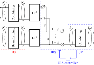
Figure 1: Schematic of the system model. The HIRS architecture adopts the model in [7].

For an incident signal ${\bf x}\in\mbox{\bb C}^{L_{\rm a}}$, the reflection and sensing signals are $\hbox{\boldmath$\Phi$}^{\sf H}{\bf x}$ and ${\bf D}^{\sf H}{\bf x}$, respectively, where

$$\Phi ={\hbox{diag}}\left(\beta_{1}e^{j\psi_{1}},\dots,\beta_{l}e^{j\psi_{l}},\dots,\beta_{L_{\rm a}}e^{j\psi_{L_{\rm a}}}\right)$$ (1)

$${\bf D} ={\hbox{diag}}\left(\bar{\beta}_{1}e^{j\rho_{1}},\dots,\bar{\beta}_{l}e^{j\rho_{l}},\dots,\bar{\beta}_{L_{\rm a}}e^{j\rho_{L_{\rm a}}}\right)$$ (2)

are $L_{\rm a}\times L_{\rm a}$ complex reflection and sensing matrices, and where for $l\in[L_{\rm a}]$ the parameter $\beta_{l}\in[0,1]$ is the amplitude of the reflection coefficients, $\psi_{l}\in[-\pi,\pi]$ is the tunable phase shift of the reflected signal, $\rho_{l}\in[-\pi,\pi]$ is the tunable phase shift for the sensed signal and $\bar{\beta}_{l}=1-\beta_{l}$.

We assume that the phase shifts can be compensated at the combining stage of the UE and thus we set $\rho_{l}=0\ \forall\ l$ in (2). For simplicity, we choose $\beta=\beta_{1}=\beta_{2}=\dots=\beta_{L_{\rm a}}$ so that

$$\hbox{\boldmath$\Phi$}(\beta,\psi) =\beta\;{\hbox{diag}}\left(e^{j\psi_{l}},\dots,e^{j\psi_{L_{\rm a}}}\right)\in\mbox{\bb C}^{L_{\rm a}\times L_{\rm a}}$$ (3)

$${\bf D}(\beta) =(1-\beta)\;{\bf I}_{L_{\rm a}}\in\mbox{\bb C}^{L_{\rm a}\times L_{\rm a}}$$ (4)

II-A Channel Model

Suppose the BS and the UE are equipped with uniform linear arrays with half-wavelength spacings (i.e. $\lambda_{c}/2$) between the antenna elements. The array response vectors at the BS and UE are denoted by

$$[{\bf a}(\theta)]_{m} =e^{j\pi(m-1)\sin(\theta)}\quad m\in[N_{\rm a}]$$ (5)

$$[{\bf b}(\phi)]_{l} =e^{j\pi(l-1)\sin(\phi)}\quad l\in[L_{\rm a}],$$ (6)

where $\theta\in[-\frac{\pi}{2},\frac{\pi}{2}]$ is the angle of arrival (AoA) or angle of departure (AoD) at the BS, and $\phi\in[-\frac{\pi}{2},\frac{\pi}{2}]$ is the AoA or AoD at the UE.

For the downlink (DL) and uplink (UL) transmission, a linear time-varying line-of-sight (LOS) channel is considered. In the delay-Doppler domain, the DL and UL channels are

$${\bf H}^{\rm dl}(\tau,\nu) =h^{\rm dl}{\bf b}(\phi){\bf a}^{\sf T}(\theta)\delta(\tau-\tau_{0}/2)\delta(\nu-\nu_{0}/2)\in\mbox{\bb C}^{L_{\rm a}\times N_{\rm a}}$$ (7)

$${\bf H}^{\rm ul}(\tau,\nu) =h^{\rm ul}{\bf a}(\theta){\bf b}^{\sf T}(\phi)\delta(\tau-\tau_{0}/2)\delta(\nu-\nu_{0}/2)\in\mbox{\bb C}^{N_{\rm a}\times L_{\rm a}}$$ (8)

where $h^{\rm dl}$ and $h^{\rm ul}$ are the attenuation coefficients, $\tau_{0}$ is the two-way delay and $\nu_{0}$ is the two-way Doppler shift.

The overall two-way channel ${\bf H}_{i}(\tau,\nu)\in\mbox{\bb C}^{N_{\rm a}\times N_{\rm a}}$ in the $i$-th slot can be written as a two-dimensional convolution as

$${\bf H}_{i}(\tau,\nu) ={\bf H}^{\rm ul}(\tau,\nu)\ast\hbox{\boldmath$\Phi$}^{\sf H}_{i}{\bf H}^{\rm dl}(\tau,\nu)$$

$$=h^{\rm dl}h^{\rm ul}{\bf a}(\theta){\bf b}^{\sf T}(\phi)\hbox{\boldmath$\Phi$}_{i}^{\sf H}{\bf b}(\phi){\bf a}^{\sf T}(\theta)\delta(\tau-\tau_{0})\delta(\nu-\nu_{0})$$

$$=h(\hbox{\boldmath$\Phi$}_{i}){\bf a}(\theta){\bf a}^{\sf T}(\theta)\delta(\tau-\tau_{0})\delta(\nu-\nu_{0}),$$ (9)

where $\hbox{\boldmath$\Phi$}_{i}$ is the reflection matrix of the IRS configured by the UE in the $i$-th slot and

$$h(\hbox{\boldmath$\Phi$}_{i})\coloneqq h^{\rm dl}h^{\rm ul}{\bf b}^{\sf T}(\phi)\hbox{\boldmath$\Phi$}^{\sf H}_{i}{\bf b}(\phi).$$ (10)

is the two-way channel coefficient.

II-B Orthogonal Frequency-Division Multiplexing Signaling

We consider multi carrier modulation with orthogonal frequency-division multiplexing (OFDM). To avoid inter-symbol interference (ISI) between OFDM symbols, each symbol is preceded by a cyclic prefix (CP) of duration $T_{\rm cp}$, resulting in an overall symbol duration of $T_{o}=T+T_{\rm cp}$. The OFDM modulated signal in the $i$-th slot is thus

$$s_{i}(t)=\sum_{n,m}x_{i}[n,m]{\sf rect}\left(\tfrac{t-nT_{o}}{T_{o}}\right)e^{j2\pi m\Delta f(t-T_{\rm cp}-nT_{o})}$$ (11)

with average power constraint

$$\mbox{\bb E}[|x_{i}[n,m]|^{2}]=P_{\rm t},\quad\forall(i,n,m)$$

We assume that pilot symbols are transmitted from the BS for the entire BA duration. For simplicity, we consider a single stream DL transmission such that we can express the beamformed transmitted signal as

$${\bf s}_{i}(t)={\bf f}\sum_{n,m}x_{i}[n,m]{\sf rect}\left(\tfrac{t-nT_{o}}{T_{o}}\right)e^{j2\pi m\Delta f(t-T_{\rm cp}-nT_{o})}$$ (12)

where ${\bf f}\in\mbox{\bb C}^{N_{\rm a}}$ is a generic beamforming (BF) vector of unit norm. We design ${\bf f}$ so that it covers a section of the beam-space with a constant gain in the main beam, and very low gain elsewhere (see [9] for details).

II-C Received Signal Model

The received signal at the UE after channel (7) is processed by the sensing matrix ${\bf D}_{i}$ and a combining matrix ${\bf U}_{i}\in\mbox{\bb C}^{L_{\rm a}\times L_{\rm rf}}$ resulting in the analog linear processing matrix ${\bf V}_{i}={\bf D}_{i}{\bf U}_{i}$. After removing the CP and applying standard OFDM processing, the sampled signal is (see e.g. [10])

$${\bf y}_{i} [n,m]=$$

$$g^{\textrm{dl}}{\bf V}_{i}^{\sf H}{\bf b}(\phi)x_{i}[n,m]e^{j2\pi(nT_{o}\frac{\nu_{0}}{2}-m\Delta f\frac{\tau_{0}}{2}})+{\bf w}_{i}[n,m],$$ (13)

where we have defined $g^{\textrm{dl}}\coloneqq h^{\rm dl}{\bf a}^{\sf T}(\theta){\bf f}$. Similarly, the received (back-scattered-) signal at the BS at the $i$-th slot is

$$\boldsymbol{r}_{i} [n,m]=$$

$$g_{i}^{\textrm{ul}}{\bf U}_{\rm BS,i}^{\sf H}{\bf b}(\theta)x_{i}[n,m]e^{j2\pi(nT_{o}\nu_{0}-m\Delta f\tau_{0})}+{\bf n}_{i}[n,m],$$ (14)

where ${\bf n}_{i}[n,m]=\frac{1}{M}\sum_{k=0}^{M-1}{\bf n}_{i}[n,k]e^{-j2\pi\frac{mk}{M}}$ is the noise after the discrete Fourier transform (DFT) with ${\bf n}_{i}[n,m]\sim{\cal N}_{{\cal C}}({\bf 0},\sigma^{2}{\bf I}_{N_{\rm rf}})$, and $g_{i}^{\textrm{ul}}\coloneqq h(\hbox{\boldmath$\Phi$}_{i}){\bf b}^{\scriptscriptstyle\mathsf{T}}(\phi){\bf f}$ the overall complex UL channel coefficient.

II-D Design of Receive Beamformers

As discussed in section II-C, the UE and BS apply a combining matrix to the signal received at their respective ULAs, due to the implemented hybrid BF architecture. To meet the page limit in this article, we provide only a brief overview of the design strategy for the sequence of combining matrices. The main concept here, is to design these matrices such that they probe different narrow angular sectors of the beam space across different slots. To this end, using a method based on solving a magnitude least-squares problem for designing BF vectors in [9, 11], we obtain a codebook of beamforming vectors $\mathcal{U}_{\text{UE}}=\{{\bf u}_{1},...,{\bf u}_{K}\}$, where each of the $k\in[K]$ codewords is a flat-top beam designed to cover a specific section on the desired field of view such that the codewords are not overlapping. In every slot $i$ of BA, the UE randomly samples $L_{\rm rf}$ BF vectors $\{\bar{{\bf u}}_{1},...,\bar{{\bf u}}_{L_{\rm rf}}\}$ from  $\mathcal{U}_{\text{UE}}$ and obtains its combining matrix, i.e. ${\bf U}_{i}=\frac{1}{\sqrt{L_{\rm rf}}}\{\bar{{\bf u}}_{1},...,\bar{{\bf u}}_{L_{\rm rf}}\}$ . A similar procedure takes place at the BS to obtain the BF vectors ${\bf U}_{\text{BS},i}$ indicated in (14).

III Beam Alignment

III-A Multi-Slot Maximum Likelihood Estimation

To solve the BA problem, both the BS and UE must estimate their AoAs. We derive a maximum likelihood (ML) scheme and, to increase the accuracy, we suppose that in a certain slot of BA all the observations up to the current slot are taken into account for the AoA estimation so that the accuracy improves over time. Since the overall complex UL channel coefficient $g_{i}^{\textrm{ul}}$ of the BS might vary in each slot due to the chosen IRS configuration, we additionally derive the multi-slot maximum likelihood estimation (MMLE) at the BS for the case of slot-wise varying complex channel coefficients. We thus first derive the multi-slot ML estimate at UE and we rewrite (13) as

$$\boldsymbol{y}_{i}[n,m]=g^{\textrm{dl}}{\bf V}_{i}^{\sf H}{\bf b}(\phi)x_{i}[n,m]t_{n,m}(\tau_{0},\nu_{0})+\boldsymbol{w}_{i}[n,m],$$ (15)

where $t_{n,m}(\tau_{0},\nu_{0})\coloneqq e^{-j\pi\left(m\Delta f\tau_{0}-nT_{o}\nu_{0}\right)}$. We can reformulate the expression of (15) by stacking the $NM$ observations into a column vector $\boldsymbol{y}_{i}\in\mbox{\bb C}^{NML_{\rm rf}}$ and, defining the expression ${\bf G}_{i}(\tau_{0},\nu_{0},\phi)\coloneqq\left({\bf T}(\tau_{0},\nu_{0})\otimes{\bf V}_{i}^{\sf H}{\bf b}(\phi)\right)$, the column vector can be defined as

$$\boldsymbol{y}_{i}=g^{\textrm{dl}}{\bf G}_{i}(\tau_{0},\nu_{0},\phi)\boldsymbol{x}_{i}+\boldsymbol{w}_{i}.$$ (16)

The likelihood-function of $\boldsymbol{y}_{i}$ is

$$L(\boldsymbol{y}_{i};(g^{\textrm{dl}},\tau_{0},\nu_{0},\phi))=\frac{1}{{\hbox{det}}(2\pi\sigma^{2}{\bf I}_{NML_{\rm rf}})^{1/2}}\cdot$$

$$\exp\left(-\frac{1}{2\sigma^{2}}\left((\boldsymbol{y}_{i}-g^{\textrm{dl}}{\bf G}_{i}\boldsymbol{x}_{i})^{\sf H}(\boldsymbol{y}_{i}-g^{\textrm{dl}}{\bf G}_{i}\boldsymbol{x}_{i})\right)\right).$$ (17)

After collecting all the previous observations up to the $i$-th slot $\boldsymbol{y}^{(i)}=[\boldsymbol{y}_{1},\dots,\boldsymbol{y}_{i}]$, the log-likelihood function is

$$\ell(\boldsymbol{y}^{(i)}; (g^{\rm dl},\tau_{0},\nu_{0},\phi))=\log\left(L(\boldsymbol{y}^{(i)};(g^{\textrm{dl}},\tau_{0},\nu_{0},\phi))\right)$$

$$=\sum_{s=1}^{i}\log\left(L(\boldsymbol{y}_{i};(g^{\textrm{dl}},\tau_{0},\nu_{0},\phi))\right).$$ (18)

Using the ML estimates for unknown parameters in [12] and

$${\bf V}_{(i)} =\sum_{s=1}^{i}\lVert\boldsymbol{x}_{s}\rVert_{2}^{2}{\bf V}_{s}{\bf V}_{s}^{\sf H}$$

$${\bf c}_{(i)}(\tau_{0},\nu_{0}) =\left[\sum_{s=1}^{i}\boldsymbol{x}_{s}^{\sf T}{\bf T}(\tau_{0},\nu_{0}){\bf Y}_{s}^{\sf H}{\bf V}_{s}^{\sf H}\right],$$

we can write the ML estimate as

$$\begin{split}(\hat{g}_{i}^{\textrm{dl}},\hat{\tau}_{i},\hat{\nu}_{i},\hat{\phi}_{i})=\operatorname*{arg\,max}_{g^{\textrm{dl}},\tau_{0},\nu_{0},\phi}{\rm Re}\left\{2g^{\textrm{dl}}{\bf c}^{\sf H}_{(i)}(\tau_{0},\nu_{0}){\bf b}(\phi)\right.\\ \left.-\big{|}g^{\textrm{dl}}\big{|}^{2}{\bf b}^{\sf H}(\phi){\bf V}_{(i)}{\bf b}(\phi)\right\}\end{split}$$ (19)

Optimizing (19) with the respect of ${\rm Re}(g^{\textrm{dl}})$ and ${\rm Im}(g^{\textrm{dl}})$, we obtain

$$g_{\textrm{opt}}^{\textrm{dl}}=\frac{{\bf b}^{\sf H}(\phi){\bf c}_{(i)}(\tau_{0},\nu_{0})}{{\bf b}^{\sf H}(\phi){\bf V}_{(i)}{\bf b}(\phi)},$$ (20)

and the ML estimates

$$(\hat{\tau}_{i},\hat{\nu}_{i},\hat{\phi}_{i})=\operatorname*{arg\,max}_{\tau_{0},\nu_{0},\phi}\frac{\left\lvert{\bf b}^{\sf H}(\phi){\bf c}_{(i)}(\tau_{0},\nu_{0})\right\rvert^{2}}{{\bf b}^{\sf H}(\phi){\bf V}_{(i)}{\bf b}(\phi)},$$ (21)

which are approximately found by evaluating the objective function in a finite set of points.

At the BS we use the same steps except that the channel coefficients in (14) depend on the slot index. We can thus rewrite the received signal (14) at the BS as

$$\boldsymbol{r}_{i}=\left(\tilde{{\bf T}}(\tau_{0},\nu_{0})\otimes g_{i}^{\rm ul}{\bf U}^{\sf H}_{\rm BS,i}{\bf a}(\theta)\right)\boldsymbol{x}_{i}+{\bf n}_{i}$$ (22)

Hence, the ML estimate $(\{\hat{g}^{\textrm{ul}}\}_{s=1}^{i},\hat{\tau}_{i},\hat{\nu}_{i},\hat{\theta}_{i})$ is

$$\begin{split}\operatorname*{arg\,min}_{\{g^{\textrm{ul}}\}_{s=1}^{i},\tau_{0},\nu_{0},\theta}{\rm Re}\left\{\sum_{s=1}^{i}\lvert g_{s}^{\rm ul}\lvert^{2}\lVert\boldsymbol{x}_{s}\lVert_{2}^{2}{\bf a}^{\sf H}(\theta){\bf U}_{\rm BS,s}{\bf U}^{\sf H}_{\rm BS,s}{\bf a}(\theta)\right.\\ \left.-2g_{s}^{\rm ul}\boldsymbol{x}^{\sf T}_{s}\tilde{{\bf T}}(\tau_{0},\nu_{0}){\bf R}_{s}^{\sf H}{\bf U}^{\sf H}_{\rm BS,s}{\bf a}(\theta)\right\},\end{split}$$ (23)

where ${\bf R}_{s}\in\mbox{\bb C}^{N_{\rm rf}\times NM}$ is the matrix of the observation at BS in the $s$-th slot. As for the UE, by defining

$$\tilde{{\bf U}}_{s} =\lVert\boldsymbol{x}_{s}\rVert_{2}^{2}{\bf U}_{\rm BS,s}{\bf U}^{\sf H}_{\rm BS,s}$$

$$\tilde{{\bf c}}_{s}(\tau_{0},\nu_{0}) =\left[\boldsymbol{x}_{s}^{\sf T}\tilde{{\bf T}}(\tau_{0},\nu_{0}){\bf R}_{s}^{\sf H}{\bf U}^{\sf H}_{\rm BS,s}\right]^{\sf H},$$ (24)

and optimizing (23) with the respect of ${\rm Re}(g_{s}^{\textrm{ul}})$ and ${\rm Im}(g_{s}^{\textrm{ul}})$, the optimal value of $g_{s}^{\textrm{ul}}$ is

$$g_{s,\textrm{opt}}^{\textrm{ul}}=\frac{{\bf a}^{\sf H}(\theta)\tilde{{\bf c}}_{s}(\tau_{0},\nu_{0})}{{\bf a}^{\sf H}(\theta)\tilde{{\bf U}}_{s}{\bf a}(\theta)},$$ (25)

which yields the ML estimates at the BS in the $i$-th slot as

$$(\hat{\tau}_{i},\hat{\nu}_{i},\hat{\theta}_{i})=\operatorname*{arg\,max}_{\tau_{0},\nu_{0},\theta}\sum_{s=1}^{i}\frac{\lvert{\bf a}^{\sf H}(\theta)\tilde{{\bf c}}_{s}(\tau_{0},\nu_{0})\lvert^{2}}{{\bf a}^{\sf H}(\theta)\tilde{{\bf U}}_{s}{\bf a}(\theta)},$$ (26)

which is approximately solved by evaluating the objective function on a finite set of points.

III-B Cramer Rao Lower Bound

We derive the CRLB as a benchmark. Let $g=|g^{\rm dl}|$ and $\psi_{g}=\angle(g^{\rm dl})$ be the amplitude and phase of $g^{\rm dl}$, respectively, and define the vector $\hbox{\boldmath$\xi$}=[g,\psi_{g},\phi,\tau^{\prime}_{0},\nu_{0}]$ with the unknown real parameters. We form the $5\times 5$ Fisher information matrix whose $(k,l)$-th element is

$$[ {\bf I}(\hbox{\boldmath$\xi$},{\bf X})]_{k,l}=$$

$$\frac{2}{\sigma^{2}}\sum_{s=1}^{i}\sum_{n,m}{\rm Re}\left\{\frac{\partial{\bf s}_{s}^{\sf H}[n,m;\hbox{\boldmath$\xi$}]}{\partial\xi_{k}}\frac{\partial{\bf s}_{s}[n,m;\hbox{\boldmath$\xi$}]}{\partial\xi_{l}}\right\},$$ (27)

where ${\bf X}=\{{\bf X}_{1},\dots,{\bf X}_{i}\}$ is the set of all pilot symbols sent up to the $i$-th slot, and ${\bf X}_{s}=\{x_{s}[n,m]\}\ \forall\ n,m$ the set of all pilot symbols sent in the $s$-th slot. The expression (27) can be manipulated to take the following structure:

$${\bf I}(\hbox{\boldmath$\xi$},{\bf X})=\frac{1}{\sigma^{2}}\begin{bmatrix}I_{gg}&0&I_{g\phi}&0&0\\ 0&I_{\psi_{g}\psi_{g}}&I_{\psi_{g}\phi}&I_{\psi_{g}\tau^{\prime}_{0}}&I_{\psi_{g}\nu_{0}}\\ I_{g\phi}&I_{\psi_{g}\phi}&I_{\phi\phi}&I_{\phi\tau^{\prime}_{0}}&I_{\phi\nu_{0}}\\ 0&I_{\psi_{g}\tau^{\prime}_{0}}&I_{\phi\tau^{\prime}_{0}}&I_{\tau^{\prime}_{0}\tau^{\prime}_{0}}&I_{\tau^{\prime}_{0}\nu_{0}}\\ 0&I_{\psi_{g}\nu_{0}}&I_{\phi\nu_{0}}&I_{\tau^{\prime}_{0}\nu_{0}}&I_{\nu_{0}\nu_{0}}\end{bmatrix},$$ (28)

Let $\hat{\phi}$ be an unbiased estimator of $\phi$. Since we consider only AoA estimation, it can be further simplified to yield the approximated CRLB in the $i$-th slot as (29), where we defined $\tilde{{\bf b}}(\phi)$ as $\tilde{{\bf b}}(\phi)={\hbox{diag}}(0,\dots,L_{\rm a}-1)\,{\bf b}(\phi)$.

$$\mathrm{Var}\{\hat{\phi}\}_{i} \geq\frac{C^{(i)}_{\phi}\sigma^{2}}{2MNP_{\rm av}g^{2}\pi^{2}\cos^{2}(\phi)\left(C^{(i)}_{\phi}\tilde{\tilde{C}}^{(i)}_{\phi}-\left({\rm Re}\left\{\tilde{C}^{(i)}_{\phi}\right\}\right)^{2}\left[3\cdot(1-\cos(\phi))^{2}+1\right]-\left({\rm Im}\left\{\tilde{C}^{(i)}_{\phi}\right\}\right)^{2}\right)}\,,~{}$$ (29)

$$\text{where}~{}~{}C^{(i)}_{\phi}\coloneqq\sum_{s=1}^{i}\|{\bf V}_{s}^{H}{\bf b}(\phi)\|_{2}^{2}~{},~{}\tilde{C}_{\phi}^{(i)}\coloneqq\sum_{s=1}^{i}\tilde{{\bf b}}^{H}(\phi){\bf V}_{s}{\bf V}_{s}^{H}{\bf b}(\phi)~{},~{}\tilde{\tilde{C}}_{\phi}^{(i)}\coloneqq\sum_{s=1}^{i}\left\lVert{\bf V}_{s}^{H}\tilde{{\bf b}}(\phi)\right\rVert_{2}^{2}.$$

III-C IRS parameter tuning

We present here a method to set the IRS parameters, namely $\beta$ and $\{\psi_{i}\}_{i=1}^{L_{\rm a}}$, in order to help the BS estimate its AoD. We define the moving standard deviation of the UE local estimate at time slot $i$ as

$$\sigma(\phi_{i-N_{\rm w}+1}^{i})\coloneqq\sqrt{\frac{1}{N_{\rm w}-1}\sum_{j=0}^{N_{\rm w}-1}\left(\hat{\phi}_{i-j}-\overline{\phi}_{i-N_{\rm w}+1}^{i}\right)^{2}},$$ (30)

where $\overline{\phi}_{i-N_{\rm w}+1}^{i}\coloneqq\frac{1}{N_{\rm w}}\sum_{j=0}^{N_{\rm w}-1}\hat{\phi}_{i-j}$ is the moving average of the estimate. Our method sets $\beta=0$ until the moving standard deviation drops below a predefined threshold, and $\beta=1$ thereafter. In particular, we select the threshold as the $3\text{\,}\mathrm{dB}$ beamwidth of an $L_{\rm a}$-antenna ULA, given by [13, Ch. 6]

$${\Theta}_{$3\text{\,}\mathrm{dB}$}=2\left[\frac{\pi}{2}-\arccos{\frac{2\cdot 1.391}{\pi L_{\rm a}}}\right].$$ (31)

Regarding the IRS phase shifts, it is trivial to observe that the magnitude of the two-way coefficient in (10) is maximized when we set $\psi_{i}=2\pi(i-1)\sin(\phi)$.

The resulting IRS configuration strategy is

$$\begin{cases}\begin{aligned} \hbox{\boldmath$\Phi$}_{i}(\beta,\psi)&={\bf 0}_{L_{\rm a}\times L_{\rm a}}\\ {\bf D}_{i}(\beta)&={\bf I}_{L_{\rm a}}\end{aligned}&{\rm if}\quad{\sigma(\phi_{i-N_{\rm w}+1}^{i}})>\Theta_{$3\text{\,}\mathrm{dB}$},\\[12.0pt] \begin{aligned} \hbox{\boldmath$\Phi$}_{i}(\beta,\psi)&={\hbox{diag}}({\bf b}(2\hat{\phi}_{i}))\\ {\bf D}_{i}(\beta)&={\bf 0}_{L_{\rm a}\times L_{\rm a}}\end{aligned}&{\rm if}\quad{\sigma(\phi_{i-N_{\rm w}+1}^{i}})<\Theta_{$3\text{\,}\mathrm{dB}$},\\ \end{cases}$$ (32)

where $\hat{\phi}_{i}$ is is the ML estimate obtained by the UE as described in section III-A.

III-D Radar Cross Section

To model the two-way channel between BS and UE, it is fundamental to consider the radar cross-section (RCS) of the IRS. In each slot $i$ of BA, the RCS of the IRS can be computed by

$$\sigma_{\rm RCS,i}\coloneqq\sigma_{\rm RCS,BBF}\cdot\cos(\phi)\cdot G_{\rm IRS}(\hbox{\boldmath$\Phi$}_{i})$$ (33)

where $\sigma_{\rm RCS,BBF}$ denotes the RCS of the IRS before BF. Given that the IRS is configured for reflection towards a certain direction, its RCS increases towards this direction by the achievable IRS gain which is defined in (10) as

$$G_{\rm IRS}(\hbox{\boldmath$\Phi$}_{i})\coloneqq|{\bf b}^{\sf T}(\phi)\hbox{\boldmath$\Phi$}^{\sf H}_{i}{\bf b}(\phi)|.$$ (34)

We propose a model for the RCS of the IRS based on [14]. This model is obtained by considering a realistic IRS array composed of conventional metallic patches. This model takes into account the physical array dimensions and the operating wavelength. The numerical value is given by

$$\sigma_{\rm RCS,BBF}=\frac{4\pi(\frac{\lambda_{c}}{2}L_{\rm a})^{2}(\frac{\lambda_{c}}{2})^{2}}{\lambda_{c}^{2}}.$$ (35)

For performance comparison purposes, we consider also a hypothetical value of RCS before BF. For this purpose, we assume the IRS fits within a conventional mobile phone. Measurements of the back of a human hand [15] or other similar-sized objects [16] show that one can obtain an average RCS between -20 dBsm and -15 dBsm. However, since such objects present curved shapes and less radar reflectivity than IRS, it is reasonable to assume that the monostatic RCS of the IRS should be higher than these values, yielding $\sigma_{\rm RCS,BBF}>-15$ dBsm. Recent work on drones’ RCS [17] found that a metallic object with an area of 128 mm $\times$ 53 mm (similar size to a mobile phone) results in a RCS value of $\sigma_{\rm RCS,MP}(\lambda_{c})=13$ dBsm at a carrier frequency $f_{c}=60$ GHz. We thus assume that $\sigma_{\rm RCS,ABF}$ after perfect BF is upper bounded as $\sigma_{\rm RCS,ABF}\leq\sigma_{\rm RCS,MP}(\lambda_{c})=13$ dBsm. To this end, we select the hypothetical value of $-5\text{\,}\mathrm{d}\mathrm{B}\mathrm{s}\mathrm{m}$ for this comparison. This value is justified since the IRS gain is upper bounded by

$$G_{\rm IRS}(\hbox{\boldmath$\Phi$}_{i})=\lvert{\bf b}^{\sf T}(\phi)\hbox{\boldmath$\Phi$}_{i}^{\sf H}{\bf b}(\phi)\lvert\leq L_{\rm a}=64\equiv$18\text{\,}\mathrm{dB}$,$$ (36)

which means $\sigma_{\rm RCS,i}$ can reach its upper bound of $13\text{\,}\mathrm{d}\mathrm{B}\mathrm{s}\mathrm{m}$ in case of $\phi=0$ and perfect reflection.

IV Numerical Results

We now provide numerical results to verify the effectiveness of the methods proposed in the previous section. In the remainder, we consider the parameters shown in Table I. The channel parameters in (7) and (8) are assumed to remain constant over $N_{\rm slot}$ slots, defined as the maximum number of slots expected to be necessary for BA. This is justified for moderate values of $N_{\rm slot}$ since the frame duration is approximately $50\text{\,}\mathrm{\SIUnitSymbolMicro s}$. Some of the results are given as a function of the SNR that would be obtained at the UE in case no beamforming would be used at the transmitter nor at the receiver. We refer to this magnitude as the SNR before beamforming (${\rm SNR}_{\rm UE,BBF}$), which is given by

$${\rm SNR}_{\rm UE,BBF}\coloneqq\frac{\lambda_{\rm c}^{2}}{(4\pi d)^{2}}\frac{P_{\rm t}}{\sigma^{2}}.$$ (37)

First, the AoA estimation accuracy at the UE side is investigated. Figure 2 shows the estimated AoA root mean square error (RMSE) as a function of SNR_UE,BBF. For evaluation of the RMSE, we run a large number of simulations over certain range of distances, where at each run, the AoA and AoD are chosen uniformly at random from the set $[-87^{\circ},87^{\circ}]$. Note that the discretization error of the ML estimation, i.e. the lowest achievable RMSE due to the discretized grid for the ML estimation in (21), is shown to evaluate the general quality of the MMLE results. It can be observed that the proposed estimation scheme improves significantly with larger number of slots for BA. We would like to further remark that, although the above simulation presents the ML estimate of the AoA, the ML estimation metrics in (21), and (26) at the UE and BS side respectively, can be used to obtain an estimate of the delay, Doppler and angle parameters simultaneously, where these parameters are defined over a 3-dimensional grid of parameters.

The following figures indicate performance in terms of the achievable spectral efficiency at the UE after obtaining angular estimates and using them to tune the beamformers. This is numerically computed by averaging

$$\log_{2}\left(1+{\rm SNR}_{\rm UE,BBF}|{\bf a}^{\sf T}(\theta){\bf a}^{*}(\hat{\theta}){\bf b}^{\sf H}(\hat{\phi}){\bf b}(\phi)|^{2}\right)$$ (38)

over multiple simulations over a range of distances, where $\hat{\phi}$ and $\hat{\theta}$ are ML estimates obtained as derived in Section III-A.

It is easy to verify that, by applying the values in Table I to (35), the RCS evaluates to approximately $-11\text{\,}\mathrm{dBsm}$. The achievable spectral efficiency after beamforming when the number of slots for BA is fixed to 32 is shown in Figure 3. There, we consider the analytic RCS, a hypothetical one, and a case where the IRS is replaced by a metallic plate of the same size. It can be observed that the communication performance after BA is close to optimal for both RCS values when the SNR is as low as $-5\text{\,}\mathrm{dB}$ to $0\text{\,}\mathrm{dB}$.

Inspired by the previous result, we now fix the ${\rm SNR}_{\rm UE,BBF}$ to $-4\text{\,}\mathrm{dB}$ (corresponding to a distance of $10\text{\,}\mathrm{m}$ for our system configuration, reasonable for indoor scenarios) and study performance in terms of achievable spectral efficiency as a function of the number of slots allocated for BA in Figure 4. The result shows that our IRS based BA method consistently improves spectral efficiency by at least $2\text{\,}\mathrm{bit}\mathrm{/}\mathrm{s}\mathrm{/}\mathrm{Hz}$. Note that in all of the above simulations we have used a relatively small transmit power of $1$mW. By using larger values, as would be the case with most BSs, the effective operational range of the scheme can be extended to meet requirements for larger cell sizes.

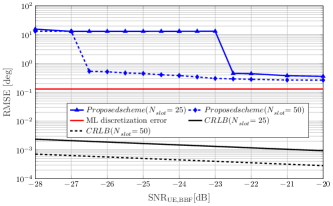
Figure 2: RMSE value of the AoA estimated at the user side.

Parameter	Value
Operating frequency	$f_{c}=$60\text{\,}\mathrm{GHz}$$ $\Leftrightarrow$ $\lambda_{\textrm{c}}=$5\text{\,}\mathrm{mm}$$
Bandwidth	$B\approx$1\text{\,}\mathrm{GHz}$$
Subcarriers	$M=2048$
Subcarrier-spacing	$\Delta f=$480\text{\,}\mathrm{kHz}$$
OFDM symbols per slot	$N=14$
CP duration	$T_{\rm cp}=0.07/{\Delta f}$
BS antennas	$N_{\rm a}=64$
IRS antennas/elements	$L_{\rm a}=64$
RF chains BS/UE	$N_{\rm rf}=L_{\rm rf}=4$
Transmit power	$P_{t}=$0\text{\,}\mathrm{d}\mathrm{B}\mathrm{m}$=$1\text{\,}\mathrm{mW}$$
Noise power	$\sigma^{2}=$-84\text{\,}\mathrm{d}\mathrm{B}\mathrm{m}$\approx$4\text{\times}{10}^{-12}\text{\,}\mathrm{W}$$
Pilot signals	similar to CSI-RS from [18]
RCS model of IRS	See (33) and (35)
ML grid size (angle, delay, Doppler)	$400\times 20\times 20$
No. of estimates for IRS activation	$N_{\textrm{w}}=5$

TABLE I: Overview of used system parameters.

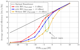
Figure 3: Averaged spectral efficiency as function of UE for different RCS values.

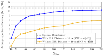
Figure 4: Achievable spectral efficiency as a function of number of estimation blocks for a fixed user at a distance of $10\text{\,}\mathrm{m}$.

V Conclusions

Motivated by the requirement for BA in mmWave communications with highly directional beamforming, we have proposed the use of an on-device-mounted HIRS to aid the BA procedure. In the proposed scheme, a multi-slot parameter estimation framework is developed to deal with the restriction imposed by the HDA architecture. Our numerical results demonstrate that with sufficiently large number of slots, the user device can reliably estimate the AoA of the incoming communication signal and maintain a significantly higher spectral efficiency.

VI Acknowledgment

The authors would like to thank Gerhard Kramer for his careful reading of the manuscript and his very useful feedback.

S. K. Dehkordi and F. Pedraza would like to acknowledge the financial support by the Federal Ministry of Education and Research of Germany in the program of “Souverän. Digital. Vernetzt.” Joint project 6G-RIC, project identification number: 16KISK030.

The research of Lorenzo Zaniboni is funded by Deutsche Forschungsgemeinschaft (DFG) through the grant KR 3517/12-1.

References

• [1] A. Liu, Z. Huang, M. Li, Y. Wan, W. Li, T. X. Han, C. Liu, R. Du, D. K. P. Tan, J. Lu, Y. Shen, F. Colone, and K. Chetty, “A survey on fundamental limits of integrated sensing and communication,” IEEE Communications Surveys & Tutorials, vol. 24, no. 2, pp. 994–1034, 2022.
• [2] F. Sohrabi and W. Yu, “Hybrid digital and analog beamforming design for large-scale antenna arrays,” IEEE Journal of Selected Topics in Signal Processing, vol. 10, no. 3, pp. 501–513, 2016.
• [3] Ö. Özdogan, E. Björnson, and E. G. Larsson, “Using intelligent reflecting surfaces for rank improvement in mimo communications,” 2020. [Online]. Available: https://arxiv.org/abs/2002.02182
• [4] Z. Esmaeilbeig, K. V. Mishra, and M. Soltanalian, “IRS-aided radar: Enhanced target parameter estimation via intelligent reflecting surfaces,” in 2022 IEEE 12th Sensor Array and Multichannel Signal Processing Workshop (SAM), 2022, pp. 286–290.
• [5] K. Meng, Q. Wu, W. Chen, and D. Li, “Intelligent surface enabled sensing-assisted communication,” 2022. [Online]. Available: https://arxiv.org/abs/2211.04200
• [6] X. Mu, Y. Liu, L. Guo, J. Lin, and R. Schober, “Simultaneously transmitting and reflecting (STAR) RIS aided wireless communications,” IEEE Transactions on Wireless Communications, vol. 21, no. 5, pp. 3083–3098, 2022.
• [7] G. C. Alexandropoulos, N. Shlezinger, I. Alamzadeh, M. F. Imani, H. Zhang, and Y. C. Eldar, “Hybrid reconfigurable intelligent metasurfaces: Enabling simultaneous tunable reflections and sensing for 6g wireless communications,” arXiv preprint arXiv:2104.04690, 2021.
• [8] I. Alamzadeh, G. C. Alexandropoulos, N. Shlezinger, and M. F. Imani, “A reconfigurable intelligent surface with integrated sensing capability,” Scientific Reports, vol. 11, no. 1, p. 20737, Oct 2021. [Online]. Available: https://doi.org/10.1038/s41598-021-99722-x
• [9] S. K. Dehkordi, L. Gaudio, M. Kobayashi, G. Caire, and G. Colavolpe, “Beam-space MIMO radar for joint communication and sensing with OTFS modulation,” IEEE Transactions on Wireless Communications, pp. 1–1, 2023.
• [10] C. Sturm and W. Wiesbeck, “Waveform design and signal processing aspects for fusion of wireless communications and radar sensing,” Proc. IEEE, vol. 99, no. 7, pp. 1236–1259, July 2011.
• [11] S. K. Dehkordi, L. Gaudio, M. Kobayashi, G. Colavolpe, and G. Caire, “Beam-space MIMO radar with OTFS modulation for integrated sensing and communications,” in 2022 IEEE International Conference on Communications Workshops (ICC Workshops), 2022, pp. 509–514.
• [12] L. L. Scharf and C. Demeure, Statistical signal processing: detection, estimation, and time series analysis.   Prentice Hall, 1991.
• [13] C. Balanis, Antenna Theory: Analysis and Design.   Wiley, 2012.
• [14] Z. Yu, C. Feng, Y. Zeng, T. Li, and S. Jin, “Wireless communication using metal reflectors: Reflection modelling and experimental verification,” 2022. [Online]. Available: https://arxiv.org/abs/2211.08626
• [15] P. Hügler, M. Geiger, and C. Waldschmidt, “RCS measurements of a human hand for radar-based gesture recognition at E-band,” in 2016 German Microwave Conference (GeMiC), 2016, pp. 259–262.
• [16] M. Shibao, K. Uchiyama, and A. Kajiwara, “RCS characteristics of road debris at 79GHz millimeter-wave radar,” in 2019 IEEE Radio and Wireless Symposium (RWS), 2019, pp. 1–4.
• [17] V. Semkin, J. Haarla, T. Pairon, C. Slezak, S. Rangan, V. Viikari, and C. Oestges, “Analyzing radar cross section signatures of diverse drone models at mmwave frequencies,” IEEE Access, vol. 8, pp. 48 958–48 969, 2020.
• [18] 5G; NR; Physical channels and modulation (3GPP TS 38.211 version 17.2.0 Release 17), 3rd Generation Partnership Project, Jun. 2022.