On the Nature of Bondi-Metzner-Sachs Transformations

Zahra Mirzaiyan$\,{}^{1}$ and Giampiero Esposito$\,{}^{2,1}$

$\,{}^{1}$ INFN Sezione di Napoli,
Complesso Universitario di Monte S. Angelo, Via Cintia Edificio 6, 80126 Napoli, Italy. $\,{}^{2}$Dipartimento di Fisica “Ettore Pancini”,
Complesso Universitario di Monte S. Angelo, Via Cintia Edificio 6, 80126 Napoli, Italy.

ABSTRACT

This paper investigates, as a first step, the four branches of BMS transformations, motivated by the classification into elliptic, parabolic, hyperbolic and loxodromic proposed a few years ago in the literature. We first prove that to each normal elliptic transformation of the complex variable $\zeta$ used in the metric for cuts of null infinity there corresponds a BMS supertranslation. We then study the conformal factor in the BMS transformation of the $u$ variable as a function of the squared modulus of $\zeta$. In the loxodromic and hyperbolic cases, this conformal factor is either monotonically increasing or monotonically decreasing as a function of the real variable given by the modulus of $\zeta$. The Killing vector field of the Bondi metric is also studied in correspondence with the four admissible families of BMS transformations. Eventually, all BMS transformations are re-expressed in the homogeneous coordinates suggested by projective geometry. It is then found that BMS transformations are the restriction to a pair of unit circles of a more general set of transformations. Within this broader framework, the geometry of such transformations is studied by means of its Segre manifold.

Type of the Paper: Article

zahra.mirzaiyan@na.infn.it, gesposito@na.infn.it.

1 Introduction

The recent developments on the applications of the Bondi-Metzner-Sachs (hereafter BMS) group, i.e., the asymptotic symmetry group of an asymptotically flat spacetime (see Eqs. (A.1)-(A.3) of the Appendix), have been motivated by black hole physics, quantum gravity and gauge theories, as is well described in many outstanding works (e.g. Refs. [1, 2, 3, 4, 5, 6, 7, 8, 9, 10, 11, 12, 13, 14, 15]. However, a purely classical investigation may still lead to a neater understanding of the mathematical operations frequently performed. Within this framework, at least four properties can be mentioned in our opinion: (i) The proof by F. Alessio and one of us [16] that the BMS group is the right semidirect product of the proper orthocronous Lorentz group ${\rm SO}^{+}(3,1)$ with supertranslations (cf. Appendix A). (ii) The division of BMS transformations into parabolic, elliptic, hyperbolic and loxodromic, since the first half of them consists of fractional linear maps which can be classified by studying their fixed points [17]. (iii) The investigation of fractional linear maps in general relativity and quantum mechanics performed in Ref. [18] (iv) The proof that the BMS group is not real analytic, and the related suggestion that it is not locally exponential [19]. (v) The recent discovery that groups of BMS type arise not only as macroscopic asymptotic symmetry groups in cosmology, but describe also a fundamental microscopic symmetry of pseudo-Riemannian geometry [20].

In the following sections, we aim at presenting a detailed investigation of the four branches of the BMS group and of yet other properties. For this purpose, Sec. $2$ defines our basic framework, Sec. $3$ obtains a new theorem on supertranslations, Sec. $4$ studies the conformal factor in the second half of BMS transformations, while Sec. $5$ studies Killing vector fields of the Bondi metric and their behaviour under BMS transformations, obtaining a novel classification. Eventually, BMS transformations in homogeneous coordinates are studied in Sec. $6$, concluding remarks are presented in Sec. $7$, while relevant details are provided in the Appendices. The reader is referred to Refs. [21, 22, 23] for the basic concepts of causal and asymptotic structure of a spacetime manifold.

2 Basic framework

The cuts of null infinity are spacelike $2$-surfaces orthogonal to the generators of null infinity. Lengths within a cut scale by a variable factor $K$ under holomorphic bijections of the $2$-sphere $S^{2}$ to itself (hereafter we use the complex variable $\zeta=e^{i\phi}\cot{\theta\over 2}$, $\phi$ and $\theta$ being the standard coordinates for $S^{2}$):

$$\zeta^{\prime}=f(\zeta)={(a\zeta+b)\over(c\zeta+d)}=f_{\Lambda}(\zeta),$$ (2.1)

where

$$\Lambda=\left(\begin{matrix}a&b\cr c&d\end{matrix}\right).$$

This is a fractional linear (or Möbius) map, and the matrix $\Lambda$ can be always taken to belong to ${\rm SL}(2,{\mathbb{C}})$, because the ratio is unaffected by rescalings of $a,b,c,d$ by the same factor, so that the passage from ${\rm GL}(2,{\mathbb{C}})$ to ${\rm SL}(2,{\mathbb{C}})$ is eventually achieved. In particular, $f_{\Lambda}(\zeta)=f_{-\Lambda}(\zeta)$, because

$${(a\zeta+b)\over(c\zeta+d)}={(-a\zeta-b)\over(-c\zeta-d)}.$$

Thus, two matrices of ${\rm SL}(2,{\mathbb{C}})$ yield the same fractional linear map if and only if the one is the opposite of the other. At this stage, we are actually dealing with the projective version of the ${\rm SL}(2,{\mathbb{C}})$ group, i.e.

$${\rm PSL}(2,{\mathbb{C}}) = \left\{(f,\Lambda)|\;f:\zeta\in{\mathbb{C}}\rightarrow f(\zeta)={(a\zeta+b)\over(c\zeta+d)},\;ad-bc=1\right\}$$ (2.2)

$$= {\rm SL}(2,{\mathbb{C}})/\delta,$$

where $\delta$ is the homeomorphism such that

$$\delta(a,b,c,d)=(-a,-b,-c,-d).$$ (2.3)

Our definition (2.2) of ${\rm PSL}(2,{\mathbb{C}})$ as a space of maps is formally analogous to the definition of ${\rm PSL}(2,{\mathbb{R}})$ by S. Katok [24], and it puts the emphasis on the fractional linear map associated to any matrix of ${\rm SL}(2,{\mathbb{C}})$. Such maps can be extended to the whole complex plane by defining [19]

$$f(\infty)={a\over c},\;f\left(-{d\over c}\right)=\infty.$$ (2.4)

By virtue of the above considerations, we can consider the equivalence relation

$$(f_{\Lambda},\Lambda)\sim(f_{\Lambda^{\prime}},\Lambda^{\prime})\Longleftrightarrow\Lambda^{\prime}=\pm\Lambda\Longrightarrow f_{\Lambda^{\prime}}(\zeta)=f_{\Lambda}(\zeta).$$

A cut remains the unit $2$-sphere under $f_{\Lambda}(\zeta)$ provided that its metric is subject to the conformal rescaling

$$K^{2}(\Lambda,\zeta)(d\theta\otimes d\theta+\sin^{2}\theta d\phi\otimes d\phi),$$ (2.5)

having defined

$$K(\Lambda,\zeta)=K_{\Lambda}(\zeta)={{1+|\zeta|^{2}}\over|a\zeta+b|^{2}+|c\zeta+d|^{2}},$$ (2.6)

where of course $|\gamma|^{2}=\gamma{\overline{\gamma}}$ for all $\gamma\in{\mathbb{C}}$. The asymptotic theory remains invariant under this rescaling provided that lengths along the generators of null infinity scale by the same amount, i.e.

$$du^{\prime}=K_{\Lambda}(\zeta)du,$$ (2.7)

which can be integrated to find

$$u^{\prime}=K_{\Lambda}(\zeta)\Bigr{[}u+\alpha(\zeta,{\overline{\zeta}})\Bigr{]},$$ (2.8)

where $\alpha$ is a suitably smooth function of $\zeta$ and of its complex conjugate ${\overline{\zeta}}$. The transformations (2.1) and (2.8) are related in such a way that they define the group of BMS transformations

$$T(\zeta)=f_{\Lambda}(\zeta)={(a\zeta+b)\over(c\zeta+d)},$$ (2.9)

$$T(u)=K_{\Lambda}(\zeta)\Bigr{[}u+\alpha(\zeta,{\overline{\zeta}})\Bigr{]}.$$ (2.10)

In a concise form, one can write [16]

$$T(\zeta,u)=(T(\zeta),T(u))=\Bigr{(}f_{\Lambda}(\zeta),K_{\Lambda}(\zeta)\Bigr{[}u+\alpha(\zeta,{\overline{\zeta}}\Bigr{]}\Bigr{)}.$$ (2.11)

As pointed out in Ref. [17], the transformations (2.9) can be classified according to their fixed points, for which $f(\zeta)=\zeta$. Hence only four families of fractional linear maps are found to exist (i) Parabolic. Only one fixed point exists, for which $(a+d)^{2}=4$, while

$$\Lambda=A_{P}=\left(\begin{matrix}\pm 1&\beta\cr 0&\pm 1\end{matrix}\right),$$ (2.12)

$$f_{\Lambda}(\zeta)=f_{P}(\zeta)=\zeta\pm\beta.$$ (2.13)

(ii) Elliptic. Two fixed points exist, for which $(a+d)^{2}<4$, while

$$\Lambda=A_{E}=\left(\begin{matrix}e^{i{\chi\over 2}}&0\cr 0&e^{-i{\chi\over 2}}\end{matrix}\right),$$ (2.14)

$$f_{\Lambda}(\zeta)=f_{E}(\zeta)=e^{i\chi}\zeta.$$ (2.15)

(iii) Hyperbolic. Two fixed points exist, for which $(a+d)^{2}>4$, while

$$\Lambda=A_{H}=\left(\begin{matrix}\sqrt{|\kappa|}&0\cr 0&{1\over\sqrt{|\kappa|}}\end{matrix}\right),$$ (2.16)

$$f_{\Lambda}(\zeta)=f_{H}(\zeta)=|\kappa|\zeta.$$ (2.17)

(iv) Loxodromic. Two fixed points exist, for which $(a+d)^{2}\in{\mathbb{C}}-{\mathbb{R}}$, and

$$(a+d)=\sqrt{k}+{1\over\sqrt{k}},\;k=\rho e^{i\sigma},\;\rho\not=1,$$

while

$$\Lambda=A_{L}=\left(\begin{matrix}\sqrt{\rho}e^{i{\sigma\over 2}}&0\cr 0&{1\over\sqrt{\rho}}e^{-i{\sigma\over 2}}\end{matrix}\right),$$ (2.18)

$$f_{\Lambda}(\zeta)=f_{L}(\zeta)=\rho e^{i\sigma}\zeta.$$ (2.19)

Note that our matrices (2.12), (2.14), (2.16) and (2.18) belong to ${\rm SL}(2,{\mathbb{C}})$, whereas in section $2$ of Ref. [17] only $A_{P}=M_{P}$ was in ${\rm SL}(2,{\mathbb{C}})$, whereas the matrices $M_{E},M_{H}$ and $M_{L}$ therein were elements of ${\rm GL}(2,{\mathbb{C}})$.

Since also the transformation $T(u)$ depends on the matrix $\Lambda$ through the conformal factor $K_{\Lambda}(\zeta)$, the work in Ref. [17] proposed the same nomenclature, from parabolic to loxodromic, for the whole group of BMS transformations in Eq. (2.11). By virtue of Eqs. (2.6) and (2.12), (2.14), (2.16) and (2.18) one finds therefore

$$K_{P}(\zeta)={{1+|\zeta|^{2}}\over\Bigr{(}1+|\pm\beta+\zeta|^{2}\Bigr{)}},$$ (2.20)

$$K_{E}(\zeta)=1,$$ (2.21)

$$K_{H}(\zeta)={|\kappa|(1+|\zeta|^{2})\over\Bigr{(}1+|\kappa|^{2}|\zeta|^{2}\Bigr{)}},$$ (2.22)

$$K_{L}(\zeta)={\rho(1+|\zeta|^{2})\over\Bigr{(}1+\rho^{2}|\zeta|^{2}\Bigr{)}},$$ (2.23)

in the parabolic, elliptic, hyperbolic and loxodromic cases, respectively. Once more, our Eqs. (2.22) and (2.23) differ by a multiplicative factor from the Eqs. in section $4$ of Ref. [17] because all our matrices are in ${\rm SL}(2,{\mathbb{C}})$.

3 A new theorem on supertranslations

At this stage, we can immediately prove the following theorem: T1. A normal elliptic transformation, where the phase factor $\chi$ in Eq. (2.15) is an integer multiple of $2\pi$, engenders a BMS supertranslation. Proof. If $\chi=2\pi l$, $l$ being a relative integer, one finds the BMS transformation

$$T(\zeta)=f_{E}(\zeta)=\zeta,$$

which implies that

$$T(\theta)=\theta,\;T(\phi)=\phi,$$ (3.1)

as well as (see Eqs. (2.10) and (2.21))

$$K_{E}(\zeta)=1\Longrightarrow T(u)=u+\alpha(\zeta,{\overline{\zeta}}).$$ (3.2)

Equations (3.1) and (3.2) are precisely the defining equations of the Abelian subgroup of supertranslations [16]. In other words, restriction to normal elliptic transformations, jointly with a choice of the function $\alpha$, engenders all supertranslations. Q.E.D.
As an explicit example, let us consider the most general metric in four dimensions in Bondi coordinates $(u,r,\zeta,{\overline{\zeta}})$:

$$g=-Udu\otimes du-e^{\beta}(du\otimes dr+dr\otimes du)+g_{AB}(dx^{A}+\frac{1}{2}U^{A}du)\otimes(dx^{B}+\frac{1}{2}U^{B}du),$$ (3.3)

where $x^{A}=(\zeta,{\overline{\zeta}})$. The local diffeomorphism invariance is fixed by the following conditions:

$$\partial_{r}\text{det}\Bigr{(}\frac{g_{AB}}{r^{2}}\Bigr{)}=0,\ \ \ \ g_{rr}=g_{rA}=0.$$ (3.4)

In order to eliminate six Lorentz generators and thereby eliminating boosts and rotations that grow with $r$ at infinity, we restrict ourselves to the diffeomorphisms generated by the vector field $\varepsilon$ whose components have the large-$r$ falloffs:

$${}^{(u)}\varepsilon,\;{}^{(r)}\varepsilon\sim\mathcal{O}(r^{0}),\ \ \ {}^{(\zeta)}\varepsilon,{}^{({\overline{\zeta}})}\varepsilon\sim\mathcal{O}(\frac{1}{r}).$$ (3.5)

By definition, the asymptotic symmetries must preserve the falloff conditions:

$$g_{uu}=-1+\frac{2m_{B}}{r}+\mathcal{O}(r^{-2}),$$

$$g_{ur}=-1+\mathcal{O}(r^{-2}),$$

$$g_{uA}=\frac{1}{2}D^{B}C_{BA}+\mathcal{O}(r^{-1}),$$

$$g_{AB}=r^{2}\gamma_{AB}+rC_{AB}+\mathcal{O}(r^{0}),$$ (3.6)

where $m_{B}$ is known as the Bondi mass aspect and $C_{\zeta\zeta}$ describes gravitational waves at large $r$. Moreover, $\gamma_{AB}$ is the metric on the 2-sphere described by

$$\gamma_{\zeta\overline{\zeta}}=\frac{2}{(1+\zeta\overline{\zeta})^{2}}.$$ (3.7)

By using the falloff conditions (3.5), one finds in Bondi gauge

$$(\mathcal{L}_{\varepsilon}g)_{rr}=2g_{ur}\partial_{r}{}^{(u)}\varepsilon,$$ (3.8)

which implies that ${}^{(u)}\varepsilon$ must be independent of $r$. In addition, to the leading order in the asymptotic expansion

$$(\mathcal{L}_{\varepsilon}g)_{ur}=g_{ur}\partial_{u}{}^{(u)}\varepsilon+\mathcal{O}(r^{-1}).$$ (3.9)

Hence, ${}^{(u)}\varepsilon(\zeta,\overline{\zeta})$ is a function on the 2-sphere which we fix as being equal to $\alpha(\zeta,\overline{\zeta})$. Then, requiring that the Bondi conditions (3.4) and the falloffs (3.6) are preserved implies that at large $r$

$$\varepsilon=\alpha(\zeta,\overline{\zeta})\ \partial_{u}+D^{\zeta}D_{\zeta}\ \alpha(\zeta,\overline{\zeta})\ \partial_{r}-\frac{1}{r}D^{\zeta}\ \alpha(\zeta,\overline{\zeta})\ \partial_{\zeta}+c.c+...,$$ (3.10)

where $\alpha(\zeta,\overline{\zeta})$ can be any function of $(\zeta,\overline{\zeta})$ on the 2-sphere. The function $\alpha(\zeta,{\overline{\zeta}})$ can be expanded in spherical harmonics on the 2-sphere. The modes $l=0$ and $l=1$ correspond to the standard global translations in Minkowski space-time. The vector field $\varepsilon(\alpha(\zeta,{\overline{\zeta}}))$ on the $l=0$ and $l=1$ spherical harmonics can be evaluated as

$$\varepsilon(Y_{0}^{0})=Y_{0}^{0}\ \partial_{u},$$

$$\varepsilon(Y_{1}^{m})=Y_{1}^{m}\ \partial_{u}+\frac{1}{2}D^{2}Y_{1}^{m}\partial_{r}-\frac{\gamma^{AB}\ \partial_{B}Y_{1}^{m}}{r}\ \partial_{A},$$ (3.11)

with the following normalization for spherical harmonics:

$$Y_{0}^{0}=1,\ \ Y_{1}^{1}=\frac{\zeta}{(1+\zeta{\overline{\zeta}})},\ \ Y_{1}^{0}=\frac{(1-\zeta{\overline{\zeta}})}{(1+\zeta{\overline{\zeta}})},\ \ Y_{1}^{-1}=\frac{\overline{\zeta}}{(1+\zeta{\overline{\zeta}})}.$$ (3.12)

Then the standard global translations in Minkowski space-time are defined as

$$\varepsilon(Y_{0}^{0})=\partial_{u},$$

$$\varepsilon(Y_{1}^{1})=\frac{\zeta}{(1+\zeta{\overline{\zeta}})}\ (\partial_{u}-\partial_{r})+\frac{\zeta^{2}}{2r}\partial_{\zeta}-\frac{1}{2r}\partial_{\overline{\zeta}},$$

$$\varepsilon(Y_{1}^{0})=\frac{(1-\zeta{\overline{\zeta}})}{(1+\zeta{\overline{\zeta}})}\ (\partial_{u}-\partial_{r})+\frac{\zeta}{r}\partial_{\zeta}-\frac{\overline{\zeta}}{r}\partial_{\overline{\zeta}},$$

$$\varepsilon(Y_{1}^{-1})=\frac{{\overline{\zeta}}}{(1+\zeta{\overline{\zeta}})}\ (\partial_{u}-\partial_{r})+\frac{1}{2r}\partial_{\zeta}-\frac{\overline{\zeta}^{2}}{2r}\partial_{\overline{\zeta}}.$$ (3.13)

Other choices of $l$ engender all supertranslations.

4 Behaviour of the conformal factor

The conformal factors (2.20), (2.22) and (2.23) have the limiting behaviours

$$\lim_{|\zeta|\to 0}K_{P}={1\over(1+|\beta|^{2})},\;\lim_{|\zeta|\to\infty}K_{P}=1,$$ (4.1)

$$\lim_{|\zeta|\to 0}K_{H}=|\kappa|,\;\lim_{|\zeta|\to\infty}K_{H}={1\over|\kappa|},$$ (4.2)

$$\lim_{|\zeta|\to 0}K_{L}=\rho,\;\lim_{|\zeta|\to\infty}={1\over\rho}.$$ (4.3)

Moreover, since the independent variable $x=|\zeta|$ is always $\geq 0$, both $K_{H}$ and $K_{L}$ can be studied by considering the function

$$F:x\in[0,\infty]\rightarrow F(x)={\xi(1+x^{2})\over(1+\xi^{2}x^{2})},$$ (4.4)

where $\xi=|\kappa|$ or $\xi=\rho$ in the hyperbolic and loxodromic cases, respectively. Since the first two derivatives of $F$ are given by

$$F^{\prime}(x)={2\xi(1-\xi^{2})x\over(1+\xi^{2}x^{2})^{2}},\;F^{\prime\prime}(x)={2\xi(1-\xi^{2})\over(1+\xi^{2}x^{2})^{3}}(1-3\xi^{2}x^{2}),$$ (4.5)

we find that, if $\xi\in]0,1[$, the function $F$ is monotonically increasing $\forall x\in[0,\infty]$, displays an upwards concavity and takes its absolute minimum at $x=0$. The figure below plots the graph of $F$ when $\xi$ is either less than $1$ or bigger than $1$.

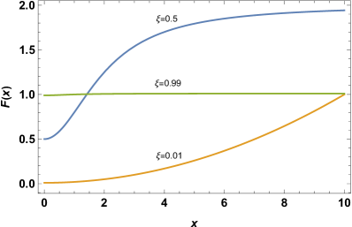
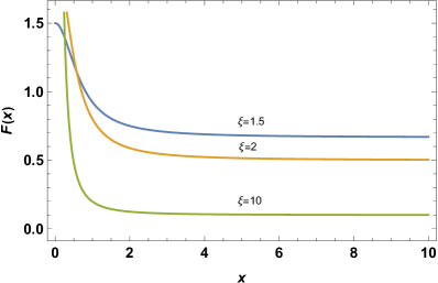
Figure 1: The conformal factor is monotonically increasing if $\xi\in]0,1[$ and monotonically decreasing if $\xi>1$ in the hyperbolic and loxodromic cases.

In the parabolic case, the conformal factor given in Eq. (2.20) can be re-expressed in the form

$$K_{P}(\zeta)={{1+|\zeta|^{2}}\over\left[1+|\beta|^{2}+\left(1\pm 2{\rm Re}\left({\beta\over\zeta}\right)\right)|\zeta|^{2}\right]},$$ (4.6)

and hence we cannot exploit the theory of functions of a real variable for the parabolic conformal factor. The figure below plots the graph of the conformal factor $K_{P}(\zeta)$ in the $(\zeta,\overline{\zeta})$ plane. Of course, using either Eq. (2.20) or Eq. (4.6) leads to the same plot ($K_{P+}$ and $K_{P-}$ are devoted to the plus-minus in the denominator of the conformal factor $K_{P}(\zeta)$).

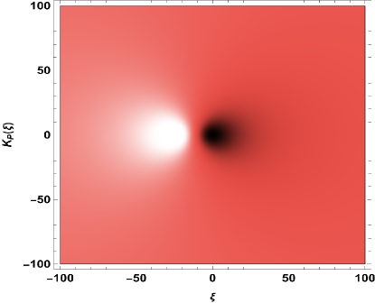
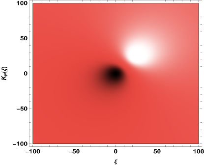
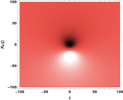
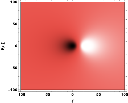
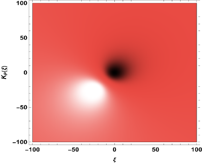
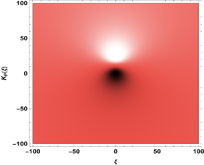
Figure 2: $K_{P}(\zeta)$ in the $(\zeta,\overline{\zeta})$ plane. First row from left to right: $K_{P+}$ with $\beta$ as a real parameter, $K_{P+}$ with $\beta$ as a complex parameter. Second row: $K_{P+}$ with $\beta$ as a purely imaginary parameter, $K_{P-}$ with $\beta$ as a real parameter. Third row: $K_{P-}$ with $\beta$ as a complex parameter, $K_{P-}$ with $\beta$ as a purely imaginary parameter.

5 Behaviour of Killing vector fields under BMS transformations

It is interesting to derive the most general form of the diffeomorphism associated with the four branches of the BMS group. We look for a diffeomorphism $\epsilon$ which satisfies the asymptotic falloff condition defined in Eq. (3.5) together with the asymptotic symmetries preserving the falloff conditions described in Eq. (3.6) in Bondi gauge. As already mentioned in Eqs. (2.9) and (2.10), the group of BMS transformations is defined as

$$T(\zeta)=f_{\Lambda}(\zeta)={(a\zeta+b)\over(c\zeta+d)}$$

$$T(u)=K_{\Lambda}(\zeta)\Bigr{[}u+\alpha(\zeta,{\overline{\zeta}})\Bigr{]}.$$ (5.1)

We recall that the first line of Eq. (5.1) can be always reduced to one of the forms (2.13), (2.15), (2.17) or (2.19), where $f_{\Lambda}(\zeta)$ reads eventually

$$f_{\Lambda}(\zeta)={\cal N}_{\gamma}\zeta+\gamma.$$

Moreover, we consider the asymptotic expansion of the vector field $\varepsilon$

$$\varepsilon={}^{(u)}\varepsilon\partial_{u}+\sum_{n=0}^{\infty}\frac{{}^{(r)}\varepsilon_{n}}{r^{n}}\partial_{r}+\sum_{n=1}^{\infty}\frac{{}^{(\zeta)}\varepsilon_{n}}{r^{n}}\partial_{\zeta}+\sum_{n=1}^{\infty}\frac{{}^{({\overline{\zeta}})}\varepsilon_{n}}{r^{n}}\partial_{\overline{\zeta}}.$$ (5.2)

The variation of the metric under a diffeomorphism is given by

$$(\mathcal{L}_{\varepsilon}g)_{\mu\nu}=\varepsilon^{\rho}\partial_{\rho}g_{\mu\nu}+g_{\mu\rho}\partial_{\nu}\varepsilon^{\rho}+g_{\nu\rho}\partial_{\mu}\varepsilon^{\rho}.$$ (5.3)

In Bondi gauge,

$$(\mathcal{L}_{\varepsilon}g)_{rr}=2g_{ur}\partial_{r}{}^{(u)}\varepsilon,$$ (5.4)

which implies that ${}^{(u)}\varepsilon$ must be independent of $r$:

$${}^{(u)}\varepsilon={}^{(u)}\varepsilon(u,\zeta,\overline{\zeta}).$$ (5.5)

By using Eq. (2.7) together with the falloff conditions for the metric, the leading order in the asymptotic expansion gives

$$(\mathcal{L}_{\varepsilon}g)_{ur}=-\partial_{u}{}^{(u)}\varepsilon=-(K_{\Lambda}(\zeta)-1),$$ (5.6)

where the last equality is obtained by evaluating the difference between the metric when $du$ is conformally rescaled according to (2.7) and the original metric with no rescaling of $du$. Equation (5.6) suggests the following form for ${}^{(u)}\varepsilon$

$${}^{(u)}\varepsilon=F(\zeta,\overline{\zeta})+u\ (K_{\Lambda}(\zeta)-1).$$ (5.7)

From $(\mathcal{L}_{\varepsilon}g)_{r\zeta}$ at order $\mathcal{O}(r^{0})$, one finds

$${}^{(\zeta)}\varepsilon_{1}=-{\cal N}_{\gamma}\ D^{\zeta}{}^{(u)}\varepsilon.$$ (5.8)

Moreover, $(\mathcal{L}_{\varepsilon}g)_{r\zeta}$ at order $\mathcal{O}(r^{-1})$ gives us

$${}^{(\zeta)}\varepsilon_{2}=\frac{{\cal N}_{\gamma}}{2}C^{\zeta\zeta}D_{\zeta}{}^{(u)}\varepsilon.$$ (5.9)

The leading order of $\mathcal{O}(r)$ term of $(\mathcal{L}_{\varepsilon}g)_{uu}$ requires

$${}^{(r)}\varepsilon_{0}=G(\zeta,\overline{\zeta})+{u\over 2}(K_{\Lambda}^{2}-1).$$ (5.10)

The function $G(\zeta,\overline{\zeta})$ can be defined from the traceless nature of the $\mathcal{O}(r)$ term of $(\mathcal{L}_{\varepsilon}g)_{\zeta\zeta}$ as

$${}^{(r)}\varepsilon_{0}=\frac{\mathcal{N}^{2}_{\gamma}}{2}D^{2}{}^{(u)}\varepsilon+{u\over 2}(K_{\Lambda}^{2}-1).$$ (5.11)

Thus, the Killing vector field of the Bondi metric in correspondence with the four branches of the BMS transformations reads as

$$\varepsilon=\big{(}F(\zeta,\overline{\zeta})+u(K_{\Lambda}(\zeta)-1)\big{)}\partial_{u}+\left(\frac{{\cal N}^{2}_{\gamma}}{2}D^{2}{}^{(u)}\varepsilon+{u\over 2}(K_{\Lambda}^{2}-1)\right)\partial_{r}$$

$$-\frac{1}{r}\big{(}{\cal N}_{\gamma}\ D^{\zeta}(F(\zeta,\overline{\zeta})+u\ (K_{\Lambda}(\zeta)-1))\big{)}\partial_{\zeta}+c.c+...$$ (5.12)

Hence four families of diffeomorphisms in correspondence with the BMS transformations exist:
(i) Parabolic. In the case of a parabolic fractional linear map for $\zeta$

$$K_{P}(\zeta)={{1+|\zeta|^{2}}\over\Bigr{(}1+|\pm\beta+\zeta|^{2}\Bigr{)}},$$ (5.13)

$${\cal N}_{\gamma}={\cal N}_{P}=\pm 1,\ \ \ \gamma=\gamma_{P}=\beta.$$ (5.14)

(ii) Elliptic. For an elliptic fractional linear map,

$$K_{E}(\zeta)=1,$$ (5.15)

$${\cal N}_{\gamma}={\cal N}_{E}=1,\ \ \ \gamma=\gamma_{E}=0.$$ (5.16)

Therefore, the Killing vector field (5.12) coincides with the form obtained in Eq. (3.10). (iii) Hyperbolic.

$$K_{H}(\zeta)={|\kappa|(1+|\zeta|^{2})\over\Bigr{(}1+|\kappa|^{2}|\zeta|^{2}\Bigr{)}},$$ (5.17)

$${\cal N}_{\gamma}={\cal N}_{H}=|k|,\ \ \ \gamma=\gamma_{H}=0.$$ (5.18)

(iv) Loxodromic.

$$K_{L}(\zeta)={\rho(1+|\zeta|^{2})\over\Bigr{(}1+\rho^{2}|\zeta|^{2}\Bigr{)}},$$ (5.19)

$${\cal N}_{\gamma}={\cal N}_{L}=\rho e^{i\sigma},\ \ \ \gamma=\gamma_{L}=0.$$ (5.20)

Thus, the Killing vector fields associated with the four branches of the BMS transformations have been here derived for the first time in the literature by substituting $K_{\Lambda}(\zeta)$, ${\cal N}_{\gamma}$ and $\gamma$ from Eqs. (5.13)-(5.20) into Eq. (5.12).

6 BMS transformations in homogeneous coordinates

The material at the beginning of Appendix B suggests expressing our complex variable $\zeta=e^{i\phi}\cot{\theta\over 2}$ in the form $\zeta={z_{0}\over\zeta_{1}}$. This is easily accomplished by defining

$$z_{0}\equiv e^{i{\phi\over 2}}\cos{\theta\over 2},\;z_{1}\equiv e^{-i{\phi\over 2}}\sin{\theta\over 2},$$ (6.1)

and hence writing the first half of BMS transformations, our Eq. (2.1), in the form (B.1):

$$\left(\begin{matrix}z_{0}^{\prime}\cr z_{1}^{\prime}\end{matrix}\right)=\left(\begin{matrix}a&b\cr c&d\end{matrix}\right)\left(\begin{matrix}z_{0}\cr z_{1}\end{matrix}\right),$$ (6.2)

where the ${\rm SL}(2,{\mathbb{C}})$ matrix can only be either (2.12), or (2.14), or (2.16), or (2.18).

The second half of BMS transformations, our Eq. (2.8), now reads as

$$u^{\prime}=K_{\Lambda}(z_{0},z_{1})\Bigr{[}u+\alpha(z_{0},z_{1};{\bar{z}}_{0},{\bar{z}}_{1})\Bigr{]},$$ (6.3)

where the conformal factor can only take one of the four forms (2.20)-(2.23), upon setting $\zeta={z_{0}\over z_{1}}$ therein.

In Eqs. (6.2) and (6.3), the complex variables are defined as in (6.1) and obey therefore the restrictions

$$|z_{0}|\leq 1,\;|z_{1}|\leq 1,$$

i.e. they correspond to a pair of unit circles $\Gamma_{0}$ and $\Gamma_{1}$. Thus, we may recognize that the BMS transformations are the restrictions to these circles of a more general set of transformations, i.e.

$$\left(\begin{matrix}w_{1}^{\prime}\cr w_{2}^{\prime}\end{matrix}\right)=\left(\begin{matrix}a&b\cr c&d\end{matrix}\right)\left(\begin{matrix}w_{1}\cr w_{2}\end{matrix}\right),$$ (6.4)

$$u^{\prime}=K_{\Lambda}(w_{1},w_{2})\Bigr{[}u+\alpha(w_{1},w_{2};{\bar{w}}_{1},{\bar{w}}_{2}\Bigr{]},$$ (6.5)

where both $w_{1}$ and $w_{2}$ belong to ${\mathbb{C}}\cup\left\{\infty\right\}$, and they are such that

$$w_{1}|_{\Gamma_{0}}=z_{0},\;w_{2}|_{\Gamma_{1}}=z_{1}.$$

Within this broader framework, one can consider two complex projective planes. Let $P$ be a point of the first plane with coordinates $(w_{0},w_{1},w_{2})$, and let $P^{\prime}$ be a point of the second plane, with coordinates $(u_{0},u_{1},u_{2})$. We can now take all nine products between a complex coordinate of $P$ and a complex coordinate of $P^{\prime}$, i.e.

$$Z_{hk}=w_{h}u_{k},\;h,k=0,1,2.$$ (6.6)

These nine complex quantities are defined up to a proportionality factor, since this is the case for both $w_{h}$ and $u_{k}$. They can be therefore interpreted as the coordinates of a point $Z$ of eight-dimensional complex projective space $S_{8}$. To the pair of points $P$ and $P^{\prime}$ there corresponds a point $Z$ of $S_{8}$ by means of Eq. (6.6). As $P$ and $P^{\prime}$ are varying in their own plane, the point $Z$ describes in $S_{8}$ a four-complex-dimensional manifold, since both $P$ and $P^{\prime}$ are varying on a plane, i.e. a two-complex-dimensional geometric object. Equations (6.6) represent therefore a four-complex-dimensional manifold $V_{4}$ in the complex projective space $S_{8}$. Such a manifold is the Segre manifold [25, 26].

If in the first plane we fix the point $P=(w_{0},w_{1},w_{2})$, Eqs. (6.6) become linear homogeneous in the $u_{k}$ coordinates and, as such, they represent a plane in $S_{8}$. Thus, to every point of the first plane there corresponds a plane on the Segre manifold $V_{4}$. The Segre manifold contains therefore a complex double infinitude of planes. In completely analogous way, another double infinitude of planes of $V_{4}$ corresponds to the double infinitude of points of the second plane. A plane of this second infinitude is obtained by fixing a point $P^{\prime}$ in the second plane and then letting $P$ vary in the first plane. Each of these $\infty^{1}$ systems of planes is an array, in light of the correspondence between elements of the system and points of a plane. Hence the Segre manifold contains two arrays of planes. Two planes of the same array do not have common points, whereas two planes belonging to different arrays have one and only one common point [25].

One can also fix the point $P$ and let the point $P^{\prime}$ vary not over the whole plane, but only on a line in such a plane. In correspondence one obtains on the Segre manifold $V_{4}$ a $V_{1}$ subset, i.e. a curve. If both $P$ and $P^{\prime}$ describe a line in their own plane, one obtains on the Segre manifold $V_{4}$ a $V_{2}$ subset, i.e. a quadric. Hence to every pair of lines there corresponds a quadric. Since there exist $\infty^{2}$ lines in a plane, the quadrics of a Segre manifold are $\infty^{4}$. In other words, the Segre manifold contains a complex fourfold infinity of quadrics.

At a deeper level, we can say that the Segre manifold is the projective image of the product of projective spaces, and it is a natural tool for studying the framework where we can accommodate the transformations that reduce to the BMS transformations upon restriction to the pair of unit circles $\Gamma_{0}$ and $\Gamma_{1}$.

7 Concluding remarks

Since asymptotic flatness is a limiting case of classical general relativity, in our opinion our work is relevant for the scope of this special issue on Extreme Regimes of Classical and Quantum Gravity Models, bearing also in mind the relevance of the BMS group for modern studies of black holes [1, 3, 4]. Moreover, we possibly fill a gap in the literature, because we have not found previous papers on the BMS group among those published in Symmetry. The original contributions of our paper are as follows. (i) Proof that to each normal elliptic transformation of the complex variable $\zeta$ used in the metric for cuts of null infinity there corresponds a BMS supertranslation. Although this might be seen as a corollary of the work initiated in Ref. [17], it has prepared the ground for the items below. (ii) Study of the conformal factor in the BMS transformation of the $u$ variable as a function of the squared modulus of $\zeta$. In the loxodromic and hyperbolic cases, such a conformal factor turns out to be either monotonically increasing or monotonically decreasing as a function of the real variable given by the absolute value of $\zeta$. In the parabolic case, the conformal factor is instead a real-valued function of complex variable, and one needs the plots of Figure $2$. (iii) A classification of Killing vector fields of the Bondi metric has been obtained in Sec. $5$. (iv) In Sec. $6$ we have found that BMS transformations are the restriction to a pair of unit circles of a more general set of transformations. Within this broader framework, the geometry of such transformations is studied by means of its Segre manifold. This provides an unforeseen bridge between the language of algebraic geometry and the analysis of BMS transformations in general relativity. (v) Our remarks at the end of Sec. $5$ might lead to a systematic application of projective geometry techniques for the definition of points at infinity in general relativity. (vi) Our results in Sec. $5$ suggest four sets of Killing fields associated with the four branches of BMS transformations. As discussed in Sec. $3$, the elliptic transformations (the case with $K_{\Lambda}(\zeta)=1$) define the Abelian subgroup of supertranslations. The linearized action of supertranslations in the Schwarzschild case is already studed in [3] which results in a black hole with linearized supertranslation hair. It would be interesting to study the action of parabolic, hyperbolic and loxodromic transformations defined by the Killing fields (5.12) on a black hole metric.

To sum up, we have addressed the physical problem of obtaining a more complete understanding of BMS diffeomorphisms of an asymptotically flat spacetime. The tools we have developed might therefore lead to new developments in black hole physics (see item (vi) above) and in the area of geometric methods in theories of gravity, especially in light of the original framework described in Sec. $6$.

Appendix A: composition of BMS transformations

It is helpful to derive, with the notation in our section $2$, the composition rule of two BMS transformations. For this purpose we note that, since a BMS transformation yields

$$T(\zeta,u)=(\zeta^{\prime},u^{\prime})=(T(\zeta),T(u)),$$ (A.1)

where

$$\zeta^{\prime}=T(\zeta)={(a\zeta+b)\over(c\zeta+d)}=f_{\Lambda}(\zeta),$$ (A.2)

$$u^{\prime}=T(u)=K_{\Lambda}(\zeta)\Bigr{[}u+\alpha(\zeta,{\overline{\zeta}})\Bigr{]},$$ (A.3)

the subsequent BMS map leads to

$$T(\zeta^{\prime},u^{\prime})=(\zeta^{\prime\prime},u^{\prime\prime})=(T(\zeta^{\prime}),T(u^{\prime})),$$ (A.4)

where, by virtue of Eq. (A2), one obtains

$$\zeta^{\prime\prime} = T(\zeta^{\prime})={(a^{\prime}\zeta^{\prime}+b^{\prime})\over(c^{\prime}\zeta^{\prime}+d^{\prime})}=f_{\Lambda^{\prime}}(\zeta^{\prime})$$ (A.5)

$$= {{(a^{\prime}a+b^{\prime}c)\zeta+(a^{\prime}b+b^{\prime}d)}\over{(c^{\prime}a+d^{\prime}c)\zeta+(c^{\prime}b+d^{\prime}d)}}={(A\zeta+B)\over(C\zeta+D)}=f_{\Lambda^{\prime\prime}}(\zeta),$$

having defined

$$\Lambda^{\prime\prime}=\left(\begin{matrix}A&B\cr C&D\end{matrix}\right)=\Lambda^{\prime}\Lambda,$$ (A.6)

which is the product of the ${\rm PSL}(2,{\mathbb{C}})$ matrices

$$\Lambda^{\prime}=\left(\begin{matrix}a^{\prime}&b^{\prime}\cr c^{\prime}&d^{\prime}\end{matrix}\right),\;\Lambda=\left(\begin{matrix}a&b\cr c&d\end{matrix}\right).$$

Moreover, one finds

$$u^{\prime\prime}=T(u^{\prime})=K_{\Lambda^{\prime}}(\zeta^{\prime})\Bigr{[}u^{\prime}+\alpha(\zeta^{\prime},{\overline{\zeta}}^{\prime})\Bigr{]}={\widetilde{K}}_{\Lambda^{\prime}\Lambda}\Bigr{[}u+{\widetilde{\alpha}}(\zeta,{\overline{\zeta}})\Bigr{]},$$ (A.7)

having defined

$${\widetilde{K}}_{\Lambda^{\prime}\Lambda}(\zeta)\equiv\Bigr{[}K_{\Lambda^{\prime}}(f_{\Lambda}(\zeta))\Bigr{]}K_{\Lambda}(\zeta),$$ (A.8)

$${\widetilde{\alpha}}(\zeta,{\overline{\zeta}})\equiv\alpha(\zeta,{\overline{\zeta}})+{\alpha\Bigr{(}f_{\Lambda}(\zeta),{\overline{f}}_{\Lambda}(\zeta)\Bigr{)}\over K_{\Lambda}(\zeta)}.$$ (A.9)

Appendix B: Origin and properties of fractional linear maps

Suppose that the pair of complex coordinates $(z_{0},z_{1})$ are mapped into the pair $(z_{0}^{\prime},z_{1}^{\prime})$ by the linear transformation

$$\left(\begin{matrix}z_{0}^{\prime}\cr z_{1}^{\prime}\end{matrix}\right)=\left(\begin{matrix}a&b\cr c&d\end{matrix}\right)\left(\begin{matrix}z_{0}\cr z_{1}\end{matrix}\right),\;ad-bc\not=0.$$ (B.1)

This means that the ratio $\zeta={z_{0}\over z_{1}}$ is mapped into

$$\zeta^{\prime}={z_{0}^{\prime}\over z_{1}^{\prime}}={(az_{0}+bz_{1})\over(cz_{0}+dz_{1})}={(a\zeta+b)\over(c\zeta+d)}.$$ (B.2)

Thus, a fractional linear map arises from a linear transformation acting on the homogeneous coordinates $z_{0},z_{1}$. For further insight, we refer the reader to the lecture notes in Ref. [27].

If the matrix on the right-hand side of Eq. (B1) pertains to ${\rm PSL}(2,{\mathbb{C}})$, the condition of unit determinant yields

$$b={(ad-1)\over c},$$ (B.3)

and hence one finds [28]

$$\zeta^{\prime}={(a\zeta+b)\over(c\zeta+d)}={{{a\over c}(c\zeta+d)-{1\over c}}\over(c\zeta+d)}={a\over c}-{1\over|c|^{2}}\left({|c|\over c}\right)^{2}{1\over\left(\zeta+{d\over c}\right)}.$$ (B.4)

Thus, half of the BMS transformations as in Eq. (A2) arise by composition of the following maps [28]:

$${\rm Translation}\;\;\zeta\rightarrow\zeta+{d\over c},$$ (B.5)

$${\rm Inversion}\;\;\zeta+{d\over c}\rightarrow{1\over\left(\zeta+{d\over c}\right)},$$ (B.6)

$${\rm Rotation}\;\;\zeta\rightarrow-\left({|c|\over c}\right)^{2}z,$$ (B.7)

$${\rm Dilation}\;\;\zeta\rightarrow{1\over|c|^{2}}\zeta,$$ (B.8)

and eventually a further translation

$$\zeta\rightarrow\zeta+{a\over c}.$$ (B.9)

The interplay of homogeneous and non-homogeneous coordinates has not been fully exploited in general relativity so far, to the best of our knowledge. For example, linear transformations among real homogeneous coordinates may be a powerful tool for studying points at infinity. In particular, one could imagine that the coordinates $x^{1},x^{2},x^{3},x^{4}$ used for a real four-dimensional Lorentzian spacetime manifold arise from five homogeneous coordinates $(y^{0},y^{1},y^{2},y^{3},y^{4})$ according to the rule

$$x^{1}={y^{1}\over y^{0}},\;x^{2}={y^{2}\over y^{0}},\;x^{3}={y^{3}\over y^{0}},\;x^{4}={y^{4}\over y^{0}},$$ (B.10)

the $y$’s being subject to the linear transformations

$${y^{\prime}}^{\mu}=\sum_{\nu=0}^{4}A_{\;\nu}^{\mu}\;y^{\nu},\;{\rm det}\left(A_{\;\nu}^{\mu}\right)\not=0,$$ (B.11)

which imply the following transformation rules for spacetime coordinates:

$${x^{\prime}}^{\mu}={\sum_{\lambda=0}^{4}A_{\;\lambda}^{\mu}\;y^{\lambda}\over\sum_{\nu=0}^{4}A_{\;\nu}^{0}\;y^{\nu}}\;\forall\mu=1,2,3,4.$$ (B.12)

The equations (B12) might provide a fully projective way of studying the concept of infinity (cf. Ref. [29]).

References

- [1] S.W. Hawking, M.J. Perry, A. Strominger, Soft hair on black holes, Phys. Rev. Lett. 116 (2016) 231301.
- [2] G. Barnich, C. Troessaert, Finite BMS transformations, JHEP 03 (2016) 167.
- [3] S.W. Hawking, M.J. Perry, A. Strominger, Superrotation charge and supertranslation hair on black holes, JHEP 05 (2017) 161.
- [4] S. Haco, S.W. Hawking, M.J. Perry, A. Strominger, Black hole entropy and soft hair, JHEP 12 (2018) 098.
- [5] A. Strominger, Lectures on the infrared structure of gravity and gauge theory (Princeton University Press, Princeton, 2018).
- [6] M. Henneaux, C. Troessaert, BMS group at spatial infinity: the Hamiltonian (ADM) approach, JHEP 03 (2018) 147.
- [7] S. Pasterski, Implications of superrotations, Phys. Rep. 829 (2019) 1.
- [8] O. Fuentealba, M. Henneaux, S. Majumdar, J. Matulich, T. Neogi, Local supersymmetry and the square roots of Bondi-Metzner-Sachs supertranslations, Phys. Rev. D 104 (2021) L121702.
- [9] E. Himwich, Z. Mirzaiyan, S. Pasterski, A note on the subleading soft graviton, JHEP 04 (2021) 172.
- [10] O. Fuentealba, M. Henneaux, J. Matulich, C. Troessaert, Bondi-Metzner-Sachs group in five spacetime dimensions, Phys. Rev. Lett. 128 (2022) 051103.
- [11] G. Barnich, K. Nguyen, R. Ruzicconi, Geometric action for extended Bondi-Metzner-Sachs group in four dimensions, JHEP 12 (2022) 154.
- [12] L. Donnay, BMS flux algebra in celestial holography, JHEP 11 (2021) 040.
- [13] C. Chowdhury, A.H. Anupam, A. Kundu, Generalized BMS algebra in higher even dimensions, Phys. Rev. D 106 (2022) 126025.
- [14] A. Bagchi, R. Kaushik, S. Pal, M. Riegler, BMS field theories with symmetry, arXiv:2209.06832 [gr-qc].
- [15] G. Compère, S.E. Gralla, An asymptotic framework for gravitational scattering, arXiv:2303.17124 [gr-qc].
- [16] F. Alessio, G. Esposito, On the structure and applications of the Bondi-Metzner-Sachs group, Int. J. Geom. Methods Mod. Phys. 15 (2018) 1830002.
- [17] G. Esposito, F. Alessio, From parabolic to loxodromic BMS transformations, Gen. Relativ. Gravit. 50 (2018) 141.
- [18] V.F. Bellino, G. Esposito, Fractional linear maps in general relativity and quantum mechanics, Int. J. Geom. Methods Mod. Phys. 18 (2021) 2150157; Erratum ibid. 18 (2021) 2192003.
- [19] D. Prinz, A. Schmeding, Lie theory for asymptotic symmetries in general relativity: The BMS group, Class. Quantum Grav. 39 (2022) 065004.
- [20] D.A. Weiss, A microscopic analogue of the BMS group, arXiv:2302.03111 [gr-qc].
- [21] S.W. Hawking, G.F.R. Ellis, The large scale structure of space-time (Cambridge University Press, Cambridge, 1973).
- [22] R. Penrose, W. Rindler, Spinors and space-time: Vol. 1, Two-spinor calculus and relativistic fields (Cambridge University Press, Cambridge, 1984).
- [23] J. Stewart, Advanced general relativity (Cambridge University Press, Cambridge, 1990).
- [24] S. Katok, Fuchsian groups (Chicago University Press, Chicago, 1992).
- [25] R. Caccioppoli, Teoria delle funzioni di più variabili complesse, edited by L. Carbone, G. Esposito, L. Dell’Aglio, G. Tomassini, Memorie dell’Accademia di Scienze Fisiche e Matematiche, Napoli, 10 (2022).
- [26] M.C. Beltrametti, E. Carletti, D. Gallarati, G. Monti Bragadin, Letture su curve, superfici e varietà proiettive speciali. Introduzione alla geometria algebrica (Bollati Boringhieri, Torino, 2003).
- [27] B. Oblak, From the Lorentz group to the celestial sphere, arXiv:1508.00920 [math-ph].
- [28] B. Maskit, Kleinian groups (Springer, Berlin, 1988).
- [29] D. Eardley, R.K. Sachs, Space-times with a future projective infinity, J. Math. Phys. 14 (1973) 209.