Braid and Phantom

Abstract.

Let $N$ be the moduli space of stable rank $2$ vector bundles on a smooth projective curve of genus $g\geq 2$ with fixed odd determinant. In [TT], we previously found a semi-orthogonal decomposition of the bounded derived category of $N$ into bounded derived categories of symmetric powers of the curve and, possibly, a phantom block. In this work, we employ the theory of weaving patterns to eliminate the possibility of a phantom, completing the proof of the decomposition conjectured by Narasimhan and, independently, by Belmans–Galkin–Mukhopadhyay.

1. Introduction

Let $N$ be the moduli space of stable rank $2$ vector bundles on a smooth projective curve of genus $g\geq 2$ with a fixed odd determinant. Let $\theta$ be an ample generator of $\operatorname{Pic}N=\mathbb{Z}$ and let $\operatorname{\mathcal{E}}$ be the Poincaré vector bundle on $C\times N$ normalized so that $\det\operatorname{\mathcal{E}}|_{\{p\}\times N}=\theta$ for every $p\in C$. The tensor vector bundles $\operatorname{\mathcal{E}}^{\boxtimes k}$ on $\operatorname{Sym}^{k}C\times N$ of rank $2^{k}$ were previously studied in [TT], where it was proved that the Fourier–Mukai functor $\operatorname{\mathcal{P}}_{\operatorname{\mathcal{E}}^{\boxtimes k}}:\,D^{b}(\operatorname{Sym}^{k}C)\to D^{b}(N)$ is fully faithful for $k\leq g-1$. In general, the image of a fully faithful Fourier–Mukai functor $\operatorname{\mathcal{P}}_{\operatorname{\mathcal{A}}}:\,D^{b}(X)\to D^{b}(Y)$ between derived categories of smooth projective varieties with kernel $\operatorname{\mathcal{A}}\in D^{b}(X\times Y)$, is an admissible subcategory of $D^{b}(Y)$, which we denote by $\langle\operatorname{\mathcal{A}}\rangle$. For example, the Beilinson semi-orthogonal decomposition can be written as $D^{b}(\operatorname{{\mathbb{P}}}^{n})=\langle\operatorname{\mathcal{O}},\ldots,\operatorname{\mathcal{O}}(n)\rangle$. With this notation, our goal is to finish the proof of the following theorem.

Theorem 1.1.

$D^{b}(N)$ has a semi-orthogonal decomposition into $D^{b}(\operatorname{Sym}^{k}C)$ (two blocks for $0\leq k\leq g-2$ and one block for $k=g-1$), arranged into four mega-blocks, and embedded by the following Fourier–Mukai functors:

$$\Bigl{\langle}\bigl{\langle}{\theta}^{1-g+k}\otimes\operatorname{\mathcal{E}}^{\boxtimes g-2-2k}\bigr{\rangle}_{0\leq k\leq\lfloor{g-2\over 2}\rfloor},\quad\bigl{\langle}{\theta}^{2-g+k}\otimes\operatorname{\mathcal{E}}^{\boxtimes g-3-2k}\bigr{\rangle}_{0\leq k\leq\lfloor{g-3\over 2}\rfloor},\quad{}$$

$${}\quad\bigl{\langle}{\theta}^{2-g+k}\otimes\operatorname{\mathcal{E}}^{\boxtimes g-2-2k}\bigr{\rangle}_{0\leq k\leq\lfloor{g-2\over 2}\rfloor},\quad\bigl{\langle}{\theta}^{2-g+k}\otimes\operatorname{\mathcal{E}}^{\boxtimes g-1-2k}\bigr{\rangle}_{0\leq k\leq\lfloor{g-1\over 2}\rfloor}\Bigr{\rangle}.$$

Within the mega-blocks, the blocks are arranged in decreasing order of $k$.

We refer to [TT] for the history of the problem and the proof of semi-orthogonality. For a slightly different decomposition used there, see Theorem 6.14. As in [TT], we work on another Fano variety, the moduli space $M$ of stable pairs $(F,s)$. Here $F$ is a stable rank $2$ vector bundle with a fixed odd determinant $\Lambda$ of degree $2g-1$, and $s\in H^{0}(C,F)$ is a non-zero section.

We play the two ray game. The variety $M$ admits a forgetful birational morphism $\zeta:\,M\to N$, $\zeta(F,s)=F$, and a birational map $\psi:\,M\dashrightarrow\operatorname{{\mathbb{P}}}^{3g-3}$, which sends a general stable pair $(F,s)\in M$ to the point of $\operatorname{{\mathbb{P}}}(\operatorname{Ext}^{1}(\Lambda,\operatorname{\mathcal{O}}))$ representing the unique extension $0\to\operatorname{\mathcal{O}}\to F\to\Lambda\to 0$ with $s\in H^{0}(C,\operatorname{\mathcal{O}})$. The map $\psi$ is factored into flips followed by a divisorial contraction [thaddeus]:

(1.1) $$M=M_{g-1}\dashrightarrow M_{g-2}\dashrightarrow\ldots\dashrightarrow M_{1}\to M_{0}=\operatorname{{\mathbb{P}}}^{3g-3}.$$

On each step $M_{k}\dashrightarrow M_{k-1}$, one projective bundle over $\operatorname{Sym}^{k}C$ is flipped into another, of smaller rank. By [TT, Proposition 3.18], this gives a semi-orthogonal decomposition of $D^{b}(M)$ with $3g-2-3k$ blocks isomorphic to $D^{b}(\operatorname{Sym}^{k}C)$ for $k=0,\ldots g-1$ and supported on the exceptional locus of the contraction $\psi:\,M\dashrightarrow\operatorname{{\mathbb{P}}}^{3g-3}$. The goal of this paper is to construct an element of the braid group on ${g(3g-1)\over 2}$ strands that mutates this semi-orthogonal decomposition into the decomposition compatible with the morphism $\zeta:\,M\to N$, which contracts a divisor $Z\subset M$ to the Brill–Noether locus $B=\{F\,|\,h^{0}(C,F)>1\}\subset N$. Some blocks go into the blocks of Theorem 1.1 (pulled back to $M$), and the rest go into the blocks of the perpendicular subcategory $\{X\,|\,R\zeta_{*}(X)=0\}\subset D^{b}(M)$, proving Theorem 1.1.

To construct the mutation, we combine vanishing theorems from [TT] with an analysis of “weaving patterns” related to various geometric constructions. The result is illustrated in Figure 1 (for genus 5). We use the term “weaving” as opposed to “braiding” to emphasize the importance of invisible wefts, which break the mutation into a sequence of standard steps. In contrast to real-world weaving, vertical warps are not parallel. When they interlace, the warp that stays above connects an admissible subcategory to itself, while the warp that goes under connects it to a differently embedded (but equivalent) subcategory. Crossing strands correspond to mutually perpendicular subcategories that both remain the same after the mutation.

Notational quirks

In complicated formulas, we follow [thaddeus] and drop the tensor product symbol, for example between line bundles. We often mix notation for line bundles and Cartier divisors, derived and underived functors (when they are the same), and denote pull-backs of vector bundles by the same letters. For example, we denote $\zeta^{*}\theta$ simply by $\theta$. Standard facts about Fourier–Mukai functors from [huybrechts] are used without much ado.

Acknowledgments

This project would have been impossible without our collaboration with Sebastián Torres [TT]. I am grateful to Alex Perry for helpful discussions and to Elias Sink for helping to fix a mistake in the earlier version of the paper. Ideas have been borrowed from the papers [myself] on Bott vanishing on GIT quotients, [castravet1, castravet2] on derived category of $\overline{M}_{0,n}$, and [toda, kosekitoda] on d-critical flips of stable pair moduli spaces. The paper was written during a visit to Imperial College in January 2023, and I thank Paolo Cascini, Alessio Corti, and Yanki Lekili for sharing an inspirational environment. The research was partially supported by the NSF grant DMS-2101726. Graphics were created by www.plainformstudio.com.

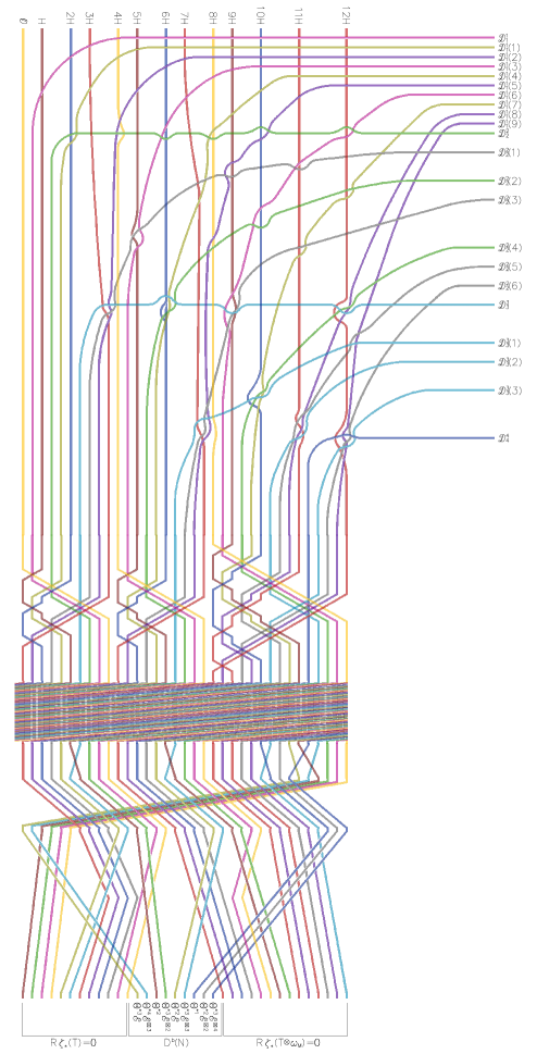
Figure 1. All weaving patterns in genus $5$          

2. Farey Twill

The Farey Twill, illustrated in Figure 2, produces an improved version of the semi-orthogonal decomposition of $D^{b}(M)$ given in [TT, Prop. 3.18]. Its blocks are isomorphic to $D^{b}(\operatorname{Sym}^{k}C)$ for $k=0,\ldots,g-1$ and are supported on the exceptional locus of the contraction $\psi:\,M\dashrightarrow\operatorname{{\mathbb{P}}}^{3g-3}$.

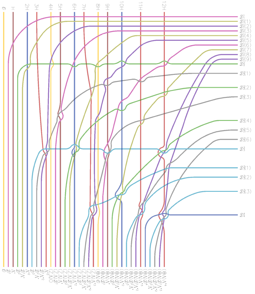
Figure 2. Farey Twill in genus $5$

The goal of this section is to prove Theorem 2.2 below, except for several lemmas, which will be proved in Section 3. We first introduce some notation, mostly from [TT] and [thaddeus], that will be used throughout the paper.

Notation 2.1.

Let $(\operatorname{\mathcal{F}},\Sigma)$ be the universal stable pair on $C\times M$. Then

$$\operatorname{\mathcal{F}}=\operatorname{\mathcal{E}}(-Z),\quad\det\operatorname{\mathcal{F}}=\Lambda\boxtimes\operatorname{{\boldsymbol{\Lambda}}},\quad\hbox{\rm and}\quad\theta=\operatorname{{\boldsymbol{\Lambda}}}(2Z),$$

where $Z$ is the exceptional divisor of the contraction $M\to N$. Let $\operatorname{\mathcal{D}}^{k}$ be the structure sheaf of a reduced subscheme

$$D^{k}=\{(D,F,s):\,s|_{D}=0\}\subset\operatorname{Sym}^{k}C\times M,$$

where we view $D\in\operatorname{Sym}^{k}C$ as a closed subscheme of $C$.

Theorem 2.2.

The Fourier–Mukai functor $\operatorname{\mathcal{P}}_{\operatorname{\mathcal{D}}^{k}}:\,D^{b}(\operatorname{Sym}^{k}C)\to D^{b}(M)$ is fully faithful for $k\leq g-1$ and $D^{b}(M)$ has a semi-orthogonal decomposition into admissible subcategories arranged into three mega-blocks, as follows:

$$\Bigl{\langle}\bigl{\langle}{\operatorname{{\boldsymbol{\Lambda}}}^{*}}^{j}\otimes\operatorname{\mathcal{D}}^{k}\bigr{\rangle}_{j+k\leq g-2\atop j,k\geq 0},\ \bigl{\langle}(Z\operatorname{{\boldsymbol{\Lambda}}}){\operatorname{{\boldsymbol{\Lambda}}}^{*}}^{j}\otimes\operatorname{\mathcal{D}}^{k}\bigr{\rangle}_{j+k\leq g-2\atop j,k\geq 0},\ \bigl{\langle}(\theta\operatorname{{\boldsymbol{\Lambda}}}){\operatorname{{\boldsymbol{\Lambda}}}^{*}}^{j}\otimes\otimes\operatorname{\mathcal{D}}^{k}\bigr{\rangle}_{j+k\leq g-1\atop j,k\geq 0}\Bigr{\rangle}.$$

Within each of the three mega-blocks, the blocks are first arranged by $j+k$ (in the increasing order) and, for a fixed $j+k$, by $j$ (in the increasing order).

Notation 2.3.

Let $E$ be the exceptional divisor of the birational morphism $M_{1}\to M_{0}=\operatorname{{\mathbb{P}}}^{3g-3}$ and let $H$ be the pullback of the hyperplane divisor. The varieties $M_{1},\ldots,M_{g-1}=M$ appearing in the sequence of flips (1.1) are isomorphic in codimension $1$. This allows us to use the same notation for their line bundles, including an important line bundle [thaddeus]

$$\operatorname{\mathcal{O}}(m,n):=(m+n)H-nE.$$

We use throughout that $M_{i}$ is the moduli space of stable pairs (for varying stability parameter) as in [thaddeus]. Mnemonically, if $(F,s)\in M_{i}$ then the scheme of zeros of $s$ in $C$ has degree at most $i$. For $0\leq k\leq i$, let $\operatorname{\mathcal{D}}_{i}^{k}$ be the structure sheaf of a reduced subscheme

$$D_{i}^{k}=\{(D,F,s):\,s|_{D}=0\}\subset\operatorname{Sym}^{k}C\times M_{i}.$$

This agrees with the definition of $D^{k}$ and $\operatorname{\mathcal{D}}^{k}$ above when $i=g-1$.

The following lemma, as well as several others, will be proved in Section 3.

Lemma 2.4.

The Fourier–Mukai functor $\operatorname{\mathcal{P}}_{\operatorname{\mathcal{D}}_{i}^{k}}:\,D^{b}(\operatorname{Sym}^{k}C)\to D^{b}(M_{i})$ is fully faithful for $0\leq k\leq i\leq g-1$.

Definition 2.5.

We introduce admissible (by Lemma 2.4) subcategories

$$\langle\operatorname{\mathcal{D}}^{k,s}_{t}\rangle\subset D^{b}(M_{\lfloor t\rfloor})$$

for integer parameters $0\leq k\leq g-1$, $0\leq s\leq 3g-3-3k$, and a real parameter $k<t<g$. Namely, $\langle\operatorname{\mathcal{D}}^{k,s}_{t}\rangle$ is the image of $\operatorname{Sym}^{k}C$ under the Fourier–Mukai functor with the kernel $\operatorname{\mathcal{D}}^{k,s}_{t}=\operatorname{\mathcal{D}}^{k}_{\lfloor t\rfloor}\otimes L^{k,s}_{t}$, where

(2.1) $$L^{k,s}_{t}=\begin{cases}\operatorname{\mathcal{O}}\left(\left\lfloor{s\over t-k}\right\rfloor,s+\left\lfloor{s\over t-k}\right\rfloor(k-1)\right)&\hbox{\rm if}\quad{\lfloor t\rfloor}>k,\cr\operatorname{\mathcal{O}}(s,sk)&\hbox{\rm if}\quad{\lfloor t\rfloor}=k.\cr\end{cases}$$

Here $\lfloor x\rfloor$ denotes the round-down of a real number $x$.

We interpret the variable $t$ as time. In the Farey Twill, named after the Farey fractions, the admissible subcategory $\langle\operatorname{\mathcal{D}}^{k,s}_{t}\rangle$ “moves” in the $(x,t)$-plane along the trajectory

(2.2) $$x_{k,s}(t)={s\over t-k},$$

with the $t$-axis pointing down and the $x$-axis to the right. On the level $t$, the blocks $\langle\operatorname{\mathcal{D}}^{k,s}_{t}\rangle\subset D^{b}(M_{{\lfloor t\rfloor}})$ are ordered by the value of the function $x_{k,s}(t)$. When the trajectories cross, the blocks mutate as will be described below. The paths of the blocks with $s=0$ have to be modified to allow them to participate in the mutations on the integer levels $t={\lfloor t\rfloor}$. The paths (2.2) (and modified paths of blocks with $s=0$) are plotted in Figure 3 in genus $5$.

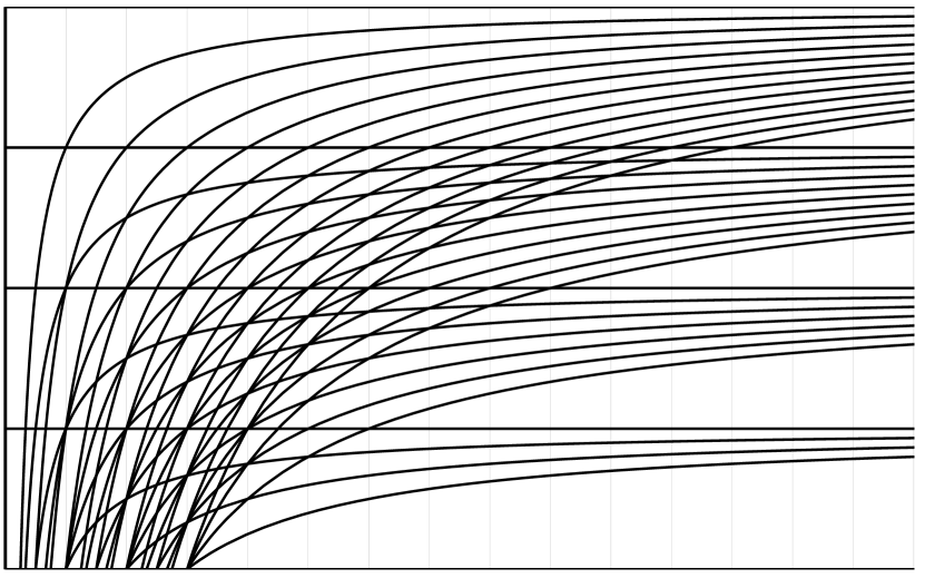
Figure 3. Genuine paths of blocks in the Farey Twill (genus $5$)

Example 2.6.

We analyze the Farey Twill for small values of $t$, see Figure 4. In this and other illustrations, we apply an $(x,t)$-plane transformation to better visualize intersections of trajectories. For examples, paths of the line bundles $H,2H,3H,\ldots$ should come from infinity (see the top of Figure 3), but in Figures 1, 2, and 4 we draw them as parallel and vertical.

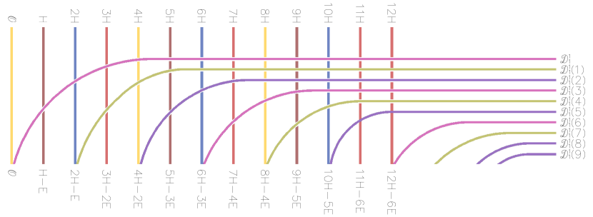
Figure 4. Starting the Farey Twill in genus $5$

$0<t<1$. $\operatorname{\mathcal{D}}^{0,s}_{t}=\operatorname{\mathcal{O}}(sH)$ and we start with the Beilinson decomposition:

$$D^{b}(M_{0})=D^{b}(\operatorname{{\mathbb{P}}}^{3g-3})=\langle\operatorname{\mathcal{O}},H,\ldots,(3g-3)H\rangle.$$

$t=1$. $\operatorname{\mathcal{D}}^{0,s}_{1}=\operatorname{\mathcal{O}}(s,0)=\operatorname{\mathcal{O}}(sH)$ but pulled back to $M_{1}$. This gives an admissible subcategory $\psi^{*}D^{b}(\operatorname{{\mathbb{P}}}^{3g-3})=\langle\operatorname{\mathcal{O}},H,\ldots,(3g-3)H\rangle\subset D^{b}(M_{1})$.

$1<t<2$. By [thaddeus], $M_{1}\simeq\operatorname{Bl}_{C}\operatorname{{\mathbb{P}}}^{3g-3}$ (where the curve $C$ is embedded in $\operatorname{{\mathbb{P}}}^{3g-3}$ by the linear system $|K_{C}+\Lambda|$) and the locus

$$D^{1}_{1}=\{(p,x)\,|\,\psi(x)=p\}\subset C\times M_{1}$$

is a projective bundle over $C$ isomorphic to the exceptional divisor $E\subset M_{1}$ via the second projection. The line bundles $\operatorname{\mathcal{O}}(s,s)$ restrict to $\operatorname{\mathcal{O}}(s)$ on the fibers $\operatorname{{\mathbb{P}}}^{3g-5}$ of the projective bundle. So the sheaves $\operatorname{\mathcal{D}}^{1,s}_{t}=\operatorname{\mathcal{D}}^{1}_{1}(s,s)$ are the Fourier–Mukai kernels that appear in the Orlov decomposition [orlov]

(2.3) $$D^{b}(M_{1})=D^{b}(\operatorname{Bl}_{C}\operatorname{{\mathbb{P}}}^{3g-3})=\langle\operatorname{\mathcal{O}},H,\ldots,(3g-3)H,\operatorname{\mathcal{D}}^{1,0}_{t},\ldots,\operatorname{\mathcal{D}}^{1,3g-6}_{t}\rangle.$$

The paths (2.2) of the new blocks $\operatorname{\mathcal{D}}^{1,s}_{t}$ come from infinity, corresponding to the fact that these blocks appear on the right in (2.3).

The sheaves $\operatorname{\mathcal{D}}^{1,s}_{t}$ don’t change when $1<t<2$ but the line bundles in (2.3) will undergo mutations as $t$ increases from $1$ to $2$. Note that $\operatorname{\mathcal{D}}^{0,s}_{1+\epsilon}=\operatorname{\mathcal{O}}(s-1,1)=\operatorname{\mathcal{O}}(sH-E)$ for $0<\epsilon\ll 1$, so these blocks have already changed compared to $t=1$. The corresponding mutations are encoded in the convention that paths of blocks with $s=0$ have to be modified to give the asymptotes of the hyperbolas (2.2). Namely, we add the horizontal line $t=1$ to the trajectory of the block $\operatorname{\mathcal{D}}^{1,0}_{t}$ and get a sequence of mutations on level $t=1$ induced by the standard short exact sequences (for $s>0$),

(2.4) $$0\to\operatorname{\mathcal{O}}(sH-E)\to\operatorname{\mathcal{O}}(sH)\to\operatorname{\mathcal{O}}_{E}(sH)\to 0.$$

This gives a semi-orthogonal decomposition of $D^{b}(M_{1})$ on the level $t=1+\epsilon$:

$$\langle\operatorname{\mathcal{O}},\operatorname{\mathcal{D}}^{1,0}_{t},H-E,2H-E,\ldots,(3g-3)H-E,\operatorname{\mathcal{D}}^{1,1}_{t},\ldots,\operatorname{\mathcal{D}}^{1,3g-6}_{t}\rangle.$$

Note that we keep the block $\operatorname{\mathcal{D}}^{1,0}_{t}$ to the right of $\operatorname{\mathcal{O}}$. Formally speaking, we modify the vertical part of its path as well (make it $x=\epsilon$ for $0<\epsilon\ll 1$).

The next block to start crossing paths in the Farey Twill is $\operatorname{\mathcal{D}}^{1,1}_{t}$, then $\operatorname{\mathcal{D}}^{1,2}_{t}$, etc. Mutations are given by the line bundle twists of (2.4), eventually giving a semi-orthogonal decomposition of $D^{b}(M_{1})$ on the level $t=2-\epsilon$:

(2.5) $$\langle\operatorname{\mathcal{O}},\operatorname{\mathcal{D}}^{1,0}_{t},H-E,2H-E,\operatorname{\mathcal{D}}^{1,1}_{t},3H-2E,4H-2E,\operatorname{\mathcal{D}}^{1,2}_{t},\ldots,\operatorname{\mathcal{D}}^{1,3g-6}_{t}\rangle.$$

with many blocks $\operatorname{\mathcal{D}}^{1,s}_{t}$ left at the end of the decomposition.

What is the advantage of (2.5) compared to (2.3)? By [TT, Section 3], we have a “windows” embedding $\iota:\,D^{b}(M_{1})\hookrightarrow D^{b}(M_{2})$ that factors as $D^{b}(M_{1})\cong\mathbb{G}_{w}\subset D^{b}(\operatorname{\mathcal{M}})\mathop{\to}\limits^{r}D^{b}(M_{2})$, where $\operatorname{\mathcal{M}}$ is an appropriate quotient stack that contains $M_{1}$ and $M_{2}$ as open substacks, $r$ is the restriction, and the windows subcategory $\mathbb{G}_{w}\subset D^{b}(\operatorname{\mathcal{M}})$ consists of complexes in equivariant derived category with cohomology sheaves having weights in the range $[0,1]$ for the wall crossing from $M_{1}$ to $M_{2}$ (see [TT, Proposition 3.18]).

The line bundles $\operatorname{\mathcal{O}},H-E,2H-E,3H-2E,4H-2E,\ldots$ appearing in (2.5) have weights $0,1,0,1,0,\ldots$ (we refer to [TT, Section 3] for the calculation of weights of all standard vector bundles), and so the windows embedding $\iota$ maps them to the same line bundles on $M_{2}$. Furthermore, $\iota$ takes the decomposition (2.5) into the following admissible subcategory:

$t=2$.

$$\langle\operatorname{\mathcal{O}},\operatorname{\mathcal{D}}^{1,0}_{2},H-E,2H-E,\operatorname{\mathcal{D}}^{1,1}_{2},3H-2E,4H-2E,\operatorname{\mathcal{D}}^{1,2}_{2},\ldots,\operatorname{\mathcal{D}}^{1,3g-6}_{2}\rangle\subset D^{b}(M_{2}).$$

$2<t<3$. We complete this admissible subcategory of $D^{b}(M_{2})$ to a semi-orthogonal decomposition of $D^{b}(M_{2})$ by adding blocks $\operatorname{\mathcal{D}}^{2,0}_{2+\epsilon},\ldots,\operatorname{\mathcal{D}}^{2,3g-9}_{2+\epsilon}$ at the end and continue with mutations encoded in intersections of paths.

To realize this program in general, we consider the “windows” embedding from [TT, Proposition 3.18],

(2.6) $$\iota:\,D^{b}(M_{i-1})\cong\mathbb{G}_{w}\subset D^{b}(\operatorname{\mathcal{M}})\mathop{\to}\limits^{r}D^{b}(M_{i}),$$

where $\operatorname{\mathcal{M}}$ is an appropriate quotient stack that contains $M_{i-1}$ and $M_{i}$ as open substacks, $r$ is the restriction, and $\mathbb{G}_{w}\subset D^{b}(\operatorname{\mathcal{M}})$ is a full subcategory of complexes in the equivariant derived category with cohomology sheaves having weights in the range $[0,i-1]$ for the wall crossing $M_{i-1}\dashrightarrow M_{i}$.

Lemma 2.7.

For $0\leq k<i$, $\operatorname{\mathcal{P}}_{\operatorname{\mathcal{D}}^{k}_{i}}=\iota\circ\operatorname{\mathcal{P}}_{\operatorname{\mathcal{D}}^{k}_{i-1}}$. Furthermore, objects in the subcategory $\langle\operatorname{\mathcal{D}}^{k}_{i-1}\rangle\subset D^{b}(M_{i-1})\cong\mathbb{G}_{w}$ have weights in the range $[0,\ldots,k]$.

Given Lemma 2.7, we claim that all subcategories $\langle\operatorname{\mathcal{D}}^{k,s}_{i-\epsilon}\rangle\subset D^{b}(M_{i-1})$ for $0<\epsilon\ll 1$ and $k<i$ map to the subcategories $\langle\operatorname{\mathcal{D}}^{k,s}_{i}\rangle\subset D^{b}(M_{i})$ under the windows embedding. More precisely, we have $\operatorname{\mathcal{P}}_{\operatorname{\mathcal{D}}^{k,s}_{i}}=\iota\circ\operatorname{\mathcal{P}}_{\operatorname{\mathcal{D}}^{k,s}_{i-\epsilon}}$. Indeed, $\operatorname{\mathcal{D}}^{k,s}_{i-\epsilon}=\operatorname{\mathcal{D}}^{k}_{i-1}\otimes L^{k,s}_{i}$ and $\operatorname{\mathcal{D}}^{k,s}_{i}=\operatorname{\mathcal{D}}^{k}_{i}\otimes L^{k,s}_{i}$, where

$$L^{k,s}_{i}=\begin{cases}\operatorname{\mathcal{O}}\left(\left\lfloor{s\over i-k}\right\rfloor,s+\left\lfloor{s\over i-k}\right\rfloor(k-1)\right)&\hbox{\rm if}\quad i-1>k,\cr\operatorname{\mathcal{O}}(s,s(i-1))&\hbox{\rm if}\quad i-1=k.\cr\end{cases}$$

The weight of $L^{k,s}_{i}$ is equal to $s\mod(i-k)$ if $i-k>1$ and 0 otherwise. In either case, the weight is less than $i-k$. So we have

$$\operatorname{\mathcal{P}}_{\operatorname{\mathcal{D}}^{k,s}_{i}}=\operatorname{\mathcal{P}}_{\operatorname{\mathcal{D}}^{k}_{i}}\otimes L^{k,s}_{i}=(\iota\circ\operatorname{\mathcal{P}}_{\operatorname{\mathcal{D}}^{k}_{i-1}})\otimes L^{k,s}_{i}=\iota\circ(\operatorname{\mathcal{P}}_{\operatorname{\mathcal{D}}^{k}_{i-1}}\otimes L^{k,s}_{i})=\iota\circ\operatorname{\mathcal{P}}_{\operatorname{\mathcal{D}}^{k,s}_{i-\epsilon}}.$$

This analysis shows that the Farey Twill is compatible with the windows embeddings $\iota:\,D^{b}(M_{i-1})\hookrightarrow D^{b}(M_{i})$.

Next, we analyze what happens when the blocks $\langle\operatorname{\mathcal{D}}^{k,s}_{t}\rangle$ and $\langle\operatorname{\mathcal{D}}^{k^{\prime},s^{\prime}}_{t}\rangle$ cross trajectories at level $t$. This happens when ${s\over t-k}={s^{\prime}\over t-k^{\prime}}$ with one exception: as explained above, we have to modify the paths of blocks $\langle\operatorname{\mathcal{D}}^{k,0}_{t}\rangle$ to be the horizontal line $t=k$ followed by the vertical line $x=k\epsilon$, $t>k$ for $0<\epsilon\ll 1$.

Lemma 2.8.

If ${s\over t-k}={s^{\prime}\over t-k^{\prime}}\not\in\operatorname{{\mathbb{Z}}}$ then $\langle\operatorname{\mathcal{D}}^{k,s}_{t}\rangle$ and $\langle\operatorname{\mathcal{D}}^{k^{\prime},s^{\prime}}_{t}\rangle$ are mutually orthogonal. Therefore, the Farey Twill at level $t$ only reorders these blocks.

Next we analyze the crossings for integer values of $x_{k,s}={s\over t-k}=n\in\operatorname{{\mathbb{Z}}}$. We have

(2.7) $$n={s\over t-k}={s-n\over t-(k+1)}={s-2n\over t-(k+2)}=\ldots={s-({\lfloor t\rfloor}-k)n\over t-{\lfloor t\rfloor}}.$$

So all the blocks $\operatorname{\mathcal{D}}^{k,s}_{t},\operatorname{\mathcal{D}}^{k+1,s-n}_{t},\operatorname{\mathcal{D}}^{k+2,s-2n}_{t},\operatorname{\mathcal{D}}^{{\lfloor t\rfloor},s-({\lfloor t\rfloor}-k)n}_{t}$ are crossing paths. If $k\geq 1$ and $s+n\leq 3g-3-3(k-1)$ then we also have $n={s+n\over t-(k-1)}$. So, without loss of generality, we may assume that (2.7) starts with the smallest possible $k$. It follows that, on the level $t$, the blocks of the subcategory

(2.8) $$\langle\operatorname{\mathcal{D}}^{k,s}_{t},\operatorname{\mathcal{D}}^{k+1,s-n}_{t},\operatorname{\mathcal{D}}^{k+2,s-2n}_{t},\ldots,\operatorname{\mathcal{D}}^{{\lfloor t\rfloor},s-({\lfloor t\rfloor}-k)n}_{t}\rangle$$

will undergo mutation that will result in the blocks

(2.9) $$\langle\operatorname{\mathcal{D}}^{{\lfloor t\rfloor},s-({\lfloor t\rfloor}-k)n}_{t+\epsilon},\ldots,\operatorname{\mathcal{D}}^{k+2,s-2n}_{t+\epsilon},\operatorname{\mathcal{D}}^{k+1,s-n}_{t+\epsilon},\operatorname{\mathcal{D}}^{k,s}_{t+\epsilon}\rangle.$$

Note the blocks are arranged in the opposite order (according to the slopes of the paths (2.2)). The twisting line bundle $\operatorname{\mathcal{O}}\left(\left\lfloor{s\over t-k}\right\rfloor,s+\left\lfloor{s\over t-k}\right\rfloor(k-1)\right)$ changes precisely when ${s\over t-k}$ decreases and passes through an integer value $n$. However, the twisting line bundle of the last block $\operatorname{\mathcal{D}}^{{\lfloor t\rfloor},s-({\lfloor t\rfloor}-k)n}_{t}$ is $\operatorname{\mathcal{O}}(s,sk)$, which is the same $\operatorname{\mathcal{D}}^{{\lfloor t\rfloor},s-({\lfloor t\rfloor}-k)n}_{t+\epsilon}$. So this block doesn’t change.

Lemma 2.9.

The mutation in $D^{b}(M_{{\lfloor t\rfloor}})$ from the semi-orthogonal decomposition (2.8) to the decomposition (2.9) is given by the following Figure 5:

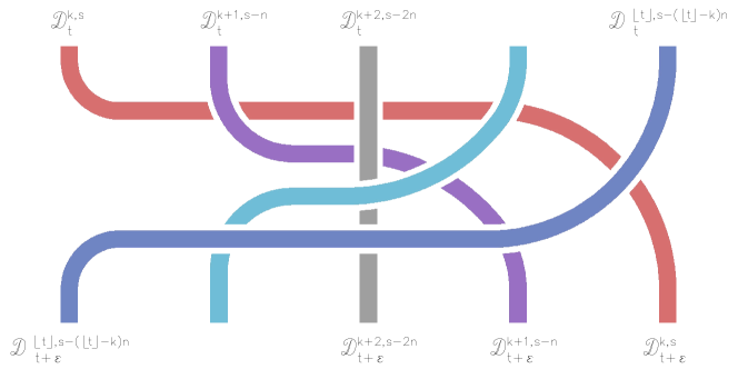
Figure 5. Basic Farey Twill Mutation

In this analysis, the case $t\in\operatorname{{\mathbb{Z}}}$ is special: the last fraction in (2.7) is $0\over 0$. Nevertheless, we still include the block $\operatorname{\mathcal{D}}^{{\lfloor t\rfloor},s-({\lfloor t\rfloor}-k)n}_{t}=\operatorname{\mathcal{D}}^{t,0}_{t}$ in the mutation according to our convention that the path of this block contains the horizontal line $t=k$. On the integer levels $t=k$, several mutations happen. Blocks participating in these mutations form several subsequences (2.8) that are disjoint, except for the last block $\operatorname{\mathcal{D}}^{k,0}_{k}$ that participates in all these mutations consecutively, starting with the rightmost subsequence of the blocks.

With these results, we can continue the Farey Twill to the level $t=g-\epsilon$ for $0<\epsilon\ll 1$, proving the following semi-orthogonal decomposition:

Corollary 2.10.

$D^{b}(M_{g-1})$ admits a semi-orthogonal decomposition

$$\left\langle\operatorname{\mathcal{D}}^{k}_{g-1}\left(\left\lfloor{s\over g-k}\right\rfloor,s+\left\lfloor{s\over g-k}\right\rfloor(k-1)\right)\right\rangle_{0\leq k\leq g-1\atop 0\leq s\leq 3g-3-3k}.$$

The blocks are arranged in the increasing order by the function ${s\over g-\epsilon-k}$.The blocks with $s=0$ are additionally ordered by $k$.

This decomposition is different from the decomposition of Theorem 2.2. To finish the proof of Theorem 2.2, we have to “undo” some of the mutations of the Farey Twill. Equivalently, we have to stop it earlier (at times that depend on the blocks). To explain the algorithm, we first employ the Farey Twill until the level $t=g-1$ (and not $t=g-\epsilon$ as in Corollary 2.10). This gives a semi-orthogonal decomposition of $D^{b}(M_{g-1})$ with blocks $\langle\operatorname{\mathcal{D}}^{k}_{g-1}\otimes L^{k,s}_{g-1}\rangle$ for $0\leq k\leq g-1$, $0\leq s\leq 3g-3-3k$, where the line bundle

$$L^{k,s}_{g-1}=\begin{cases}\operatorname{\mathcal{O}}\left(\left\lfloor{s\over g-1-k}\right\rfloor,s+\left\lfloor{s\over g-1-k}\right\rfloor(k-1)\right)&\hbox{\rm if}\quad k<g-1,\cr\operatorname{\mathcal{O}}&\hbox{\rm if}\quad k=g-1.\cr\end{cases}$$

Note that the block $\operatorname{\mathcal{D}}^{g-1,0}_{g-1}$ has not participated in the Farey Twill yet. On the level $t=g-1$, we do a single additional chain mutation of Lemma 2.9, from the sequence of blocks $\langle\operatorname{\mathcal{D}}^{0,3g-3}_{g-1},\operatorname{\mathcal{D}}^{1,3g-6}_{g-1},\ldots,\operatorname{\mathcal{D}}^{g-2,3}_{g-1},\operatorname{\mathcal{D}}^{g-1,0}_{g-1}\rangle$ to the sequence of blocks $\langle\operatorname{\mathcal{D}}^{g-1,0}_{g-1},\operatorname{\mathcal{D}}^{g-2,3}_{g-1+\epsilon},\ldots,\operatorname{\mathcal{D}}^{1,3g-6}_{g-1+\epsilon},\operatorname{\mathcal{D}}^{0,3g-3}_{g-1+\epsilon}\rangle$. This gives precisely the very last blocks $\bigl{\langle}\operatorname{\mathcal{D}}^{k}(2,2g-4+j)\bigr{\rangle}_{j+k=g-1\atop j,k\geq 0}$ of the third mega-block of Theorem 2.2, in the correct order.

It remains to explain how to obtain the remaining blocks in Theorem 2.2. These blocks are arranged into three mega-blocks

$$\Bigl{\langle}\bigl{\langle}\operatorname{\mathcal{D}}^{k}(0,j)\bigr{\rangle},\quad\bigl{\langle}\operatorname{\mathcal{D}}^{k}(1,g-2+j\bigr{\rangle},\quad\bigl{\langle}\operatorname{\mathcal{D}}^{k}(2,2g-4+j)\bigr{\rangle}\Bigr{\rangle}$$

that appear on the left of the semi-orthogonal decomposition. In each of the three mega-blocks, $j,k\geq 0$, $j+k\leq g-2$, and the blocks are first arranged by $j+k$ and then by $j$ (both in the increasing order).

These blocks will come from the blocks $\langle\operatorname{\mathcal{D}}^{k,s}_{g-1}\rangle$ of the Farey Twill with $0\leq k\leq g-2$, $0\leq s\leq 3g-4-3k$. The idea is to stop the Farey Twill for the block $\langle\operatorname{\mathcal{D}}^{k,s}_{g-1}\rangle$ shortly after $\left\lfloor{s\over g-1-k}\right\rfloor$ reaches its minimum, since afterwards this block no longer changes. We will also ensure that it will no longer participate in mutations of other blocks. Concretely, we choose the stopping time $t=t(s,k)$ as follows:

$${s\over t-k}=\left\lfloor{s\over g-1-k}\right\rfloor+{j+k\over g-1},\quad\hbox{\rm where}\quad j=s-\left\lfloor{s\over g-1-k}\right\rfloor(g-1-k).$$

After this time $t(s,k)$, the Farey Twill path is contained in the vertical strip ${s\over t-k}\in[0,1)$, $[1,2)$, or $[2,3)$, depending on the value of $\left\lfloor{s\over g-1-k}\right\rfloor=0,1$, or $2$. So the blocks no longer mutate in the Farey Twill, only permute. Instead of doing these permutations, we just order the blocks by the value of ${s\over t(s,k)-k}$, or equivalently by $j+k$, within each of the three mega-blocks. When $j+k$ is the same, the values of the stopping time $t(s,k)$ are different, with the larger value of $j$ corresponding to the larger value of $t$. It follows that the blocks with the same $j+k$ are ordered by $j$ in the increasing order.

3. Cross Warp

In this section we will study a rather striking weaving pattern in $D^{b}(M)$, which is illustrated in Figure 6 (in genus $5$). We call it the Cross Warp.

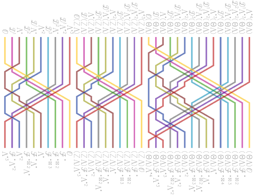
Figure 6. Cross Warp in genus $5$

Theorem 3.1 below provides a semi-orthogonal decomposition of $D^{b}(M)$ with blocks embedded by Fourier–Mukai functors with the kernels given by the tensor vector bundles $\operatorname{\mathcal{F}}^{*\boxtimes k}$ on $\operatorname{Sym}^{k}C\times M$ (twisted by line bundles). We refer to [TT, Section 2] for basic properties of tensor vector bundles. The semi-orthogonal decompositions of Theorem 2.2 and Theorem 3.1 are connected by the Cross Warp pattern illustrated in Figure 6 (in genus $5$).

Theorem 3.1.

$D^{b}(M)$ has a semi-orthogonal decomposition into admissible subcategories arranged into three mega-blocks, as follows:

$$\Bigl{\langle}\bigl{\langle}{\operatorname{{\boldsymbol{\Lambda}}}^{*}}^{k}{\operatorname{\mathcal{F}}^{*\boxtimes j}}\bigr{\rangle}_{j+k\leq g-2\atop j,k\geq 0},\ \bigl{\langle}{(Z\operatorname{{\boldsymbol{\Lambda}}})\operatorname{{\boldsymbol{\Lambda}}}^{*}}^{k}{\operatorname{\mathcal{F}}^{*\boxtimes j}}\bigr{\rangle}_{j+k\leq g-2\atop j,k\geq 0},\ \bigl{\langle}{(\theta\operatorname{{\boldsymbol{\Lambda}}})\operatorname{{\boldsymbol{\Lambda}}}^{*}}^{k}{\operatorname{\mathcal{F}}^{*\boxtimes j}}\bigr{\rangle}_{j+k\leq g-1\atop j,k\geq 0}\Bigr{\rangle}.$$

Within each of the three mega-blocks, the blocks are arranged first by $k$ (in the decreasing order) and then, for a fixed $k$, by $j$ (in the decreasing order).

The proof is a simple corollary of the following theorem, which will also imply several lemmas that were needed in Section 2.

Theorem 3.2.

The Fourier–Mukai functors $\operatorname{\mathcal{P}}_{\operatorname{\mathcal{D}}_{i}^{k}}:\,D^{b}(\operatorname{Sym}^{k}C)\to D^{b}(M_{i})$ introduced in Section 2 have the following properties:

1. $\operatorname{\mathcal{P}}_{\operatorname{\mathcal{D}}_{i}^{k}}$ is fully faithful for $0\leq k\leq i\leq g-1$.

2. For $k\leq i-1$, $\iota\circ\operatorname{\mathcal{P}}_{\operatorname{\mathcal{D}}_{i-1}^{k}}=\operatorname{\mathcal{P}}_{\operatorname{\mathcal{D}}_{i}^{k}}$, where $\iota$ is the embedding (2.6).

3. The Fourier–Mukai functors $\operatorname{\mathcal{P}}_{\operatorname{\mathcal{D}}_{i}^{k}},\ \operatorname{\mathcal{P}}_{\operatorname{\mathcal{F}}^{*\boxtimes k}}:\,D^{b}(\operatorname{Sym}^{k}C)\to D^{b}(M_{i})$ are related via the Cross Warp mutation illustrated in Figure 7.

   

   Figure 7. Basic Cross Warp Mutation

We will first prove various corollaries of Theorem 3.2 and introduce additional notation, before proving the theorem itself in the next section.

Proof of Theorem 3.1.

Each of the three mega-blocks of the semi-orthogonal decomposition of Theorem 2.2 mutates into the corresponding mega-block of the decomposition of Theorem 3.1, without any interaction between the mega-blocks. Furthermore, the second (resp., third) mega-block differ from the first one by a twist with the line bundle $Z\otimes\operatorname{{\boldsymbol{\Lambda}}}$ (resp., $\theta\otimes\operatorname{{\boldsymbol{\Lambda}}}$). In addition, the third mega-block is larger (it includes the kernel with $\operatorname{\mathcal{D}}^{g-1}$ whereas the first two mega-blocks continue only up to $\operatorname{\mathcal{D}}^{g-2}$). So it is enough to describe the mutation for the first mega-block, which is illustrated in Figure 8.

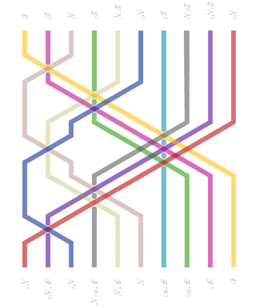
Figure 8. First mega-block of the Cross Warp in genus $5$

The Cross Warp mutation of Theorem 3.2 (c) is designed so that these mutations stack on top of each other. More precisely, the mutation with $\operatorname{\mathcal{D}}^{k}$ at the top in the middle connects to the mutation with $\operatorname{\mathcal{D}}^{k-1}$ on the top left and with the mutation with $\operatorname{\mathcal{D}}^{k-1}\otimes\operatorname{{\boldsymbol{\Lambda}}}^{*}$ on the bottom left. This gives the Cross Warp pattern, where we indicate the top middles of each block:

$$\begin{matrix}\operatorname{\mathcal{O}}\cr&\ldots&\cr\ldots&&\operatorname{\mathcal{D}}^{g-5}&&&\cr&\ldots&&\operatorname{\mathcal{D}}^{g-4}&&\cr\ldots&&\operatorname{\mathcal{D}}^{g-5}\operatorname{{\boldsymbol{\Lambda}}}^{*}&&\operatorname{\mathcal{D}}^{g-3}&\cr&\ldots&&\operatorname{\mathcal{D}}^{g-4}\operatorname{{\boldsymbol{\Lambda}}}^{*}&&\operatorname{\mathcal{D}}^{g-2}\cr\ldots&&\operatorname{\mathcal{D}}^{g-5}{\operatorname{{\boldsymbol{\Lambda}}}^{*}}^{2}&&\operatorname{\mathcal{D}}^{g-3}\operatorname{{\boldsymbol{\Lambda}}}^{*}&\cr&\ldots&&\operatorname{\mathcal{D}}^{g-4}{\operatorname{{\boldsymbol{\Lambda}}}^{*}}^{2}&&\cr\ldots&&\operatorname{\mathcal{D}}^{g-5}{\operatorname{{\boldsymbol{\Lambda}}}^{*}}^{3}&&&\cr&\ldots&\cr{\operatorname{{\boldsymbol{\Lambda}}}^{*}}^{g-2}\cr\end{matrix}$$

Altogether this gives the mutation from the semi-orthogonal decomposition

$$\langle\operatorname{\mathcal{O}}\rangle,\langle\operatorname{\mathcal{D}}^{1},\operatorname{{\boldsymbol{\Lambda}}}^{*}\rangle,\langle\operatorname{\mathcal{D}}^{2},\operatorname{\mathcal{D}}^{1}\operatorname{{\boldsymbol{\Lambda}}}^{*},{\operatorname{{\boldsymbol{\Lambda}}}^{*}}^{2}\rangle,\ldots,\langle\operatorname{\mathcal{D}}^{g-2},\operatorname{\mathcal{D}}^{g-3}{\operatorname{{\boldsymbol{\Lambda}}}^{*}},\ldots,\operatorname{\mathcal{D}}^{1}{\operatorname{{\boldsymbol{\Lambda}}}^{*}}^{g-3},{\operatorname{{\boldsymbol{\Lambda}}}^{*}}^{g-2}\rangle$$

of Theorem 2.2 to the semi-orthogonal decomposition

$$\langle{\operatorname{{\boldsymbol{\Lambda}}}^{*}}^{g-2}\rangle,\langle\operatorname{\mathcal{F}}^{*}{\operatorname{{\boldsymbol{\Lambda}}}^{*}}^{g-3},{\operatorname{{\boldsymbol{\Lambda}}}^{*}}^{g-3}\rangle,,\ldots,\langle{\operatorname{\mathcal{F}}^{*\boxtimes g-2}},{\operatorname{\mathcal{F}}^{*\boxtimes g-3}},\ldots,\operatorname{\mathcal{F}}^{*},\operatorname{\mathcal{O}}\rangle$$

of Theorem 3.1. The other two mega-blocks differ by line bundle twists. ∎

Proof of Lemma 2.4.

This is a reformulation of Theorem 3.2 (a). ∎

Proof of Lemma 2.7.

The first part is a reformulation of Theorem 3.2 (b). The second part follows from Theorem 3.2 (c) and induction on $k$, since the weights of the vector bundles $\operatorname{\mathcal{F}}^{*\boxtimes j}$ are in $[0,j]$ by [TT, Section 2]. ∎

Notation 3.3.

In addition to $\operatorname{Sym}^{k}C$, we work on $C^{k}$. The $S_{k}$-quotient

$$\tau:\,C^{k}\times M_{i}\to\operatorname{Sym}^{k}C\times M_{i}$$

commutes with arbitrary base change [TT, Section 2]. To avoid confusing objects on $\operatorname{Sym}^{k}C\times M_{i}$ and $C^{k}\times M_{i}$, we adorn the latter with the hat.For example, $\hat{\operatorname{\mathcal{F}}}^{*\boxtimes k}=\pi_{1}^{*}\operatorname{\mathcal{F}}^{*}\otimes\ldots\otimes\pi_{k}^{*}\operatorname{\mathcal{F}}^{*}$ and $\operatorname{\mathcal{F}}^{*\boxtimes k}=\tau^{S_{k}}_{*}\left(\hat{\operatorname{\mathcal{F}}}^{{}^{*}\boxtimes k}\right)$. Let

$$\bar{\operatorname{\mathcal{F}}}^{\boxtimes k}:=\tau^{S_{k}}_{*}\bigl{(}({\hat{\operatorname{\mathcal{F}}}}^{\boxtimes k})\otimes\operatorname{sgn}\bigr{)},$$

where $\operatorname{sgn}$ is the sign representation of $S_{k}$

Lemma 3.4.

We have the following formulas:

$$\operatorname{\mathcal{F}}^{*\boxtimes k}\simeq(\Lambda^{*\boxtimes k}\boxtimes\operatorname{{\boldsymbol{\Lambda}}}^{*k})\otimes\operatorname{\mathcal{F}}^{\boxtimes k},$$

$$(\operatorname{\mathcal{F}}^{*\boxtimes k})^{*}\simeq\bar{\operatorname{\mathcal{F}}}^{\boxtimes k}(\Delta/2),$$

where $\operatorname{\mathcal{O}}(-\Delta/2)=\tau_{*}^{S_{k}}(\operatorname{\mathcal{O}}\otimes\operatorname{sgn})$ is a line bundle on $\operatorname{Sym}^{k}C$ such that $\operatorname{\mathcal{O}}(-\Delta/2)^{\otimes 2}\simeq\operatorname{\mathcal{O}}(-\Delta)$, where $\Delta\subset\operatorname{Sym}^{k}C$ is the diagonal divisor.

Proof.

By [DN, Theorem 2.3], $\Lambda^{*\boxtimes k}$ is a descent of $\hat{\Lambda}^{*\boxtimes k}$. So we have $\operatorname{\mathcal{F}}^{*\boxtimes k}=\tau^{S_{k}}_{*}\left((\hat{\Lambda}^{*\boxtimes k}\boxtimes\operatorname{{\boldsymbol{\Lambda}}}^{*k})\otimes\hat{\operatorname{\mathcal{F}}}^{\boxtimes k}\right)\simeq(\Lambda^{*\boxtimes k}\boxtimes\operatorname{{\boldsymbol{\Lambda}}}^{*k})\otimes\tau^{S_{k}}_{*}\left(\hat{\operatorname{\mathcal{F}}}\right)^{\boxtimes k}$ by projection formula. The latter expression is equal to $(\Lambda^{*\boxtimes k}\boxtimes\operatorname{{\boldsymbol{\Lambda}}}^{*k})\otimes\operatorname{\mathcal{F}}^{\boxtimes k}$.

The morphism $\tau$ is ramified along $B=\tau^{-1}(\Delta)$ generically of order $2$. So $\operatorname{\mathcal{O}}(B)$ is a relative dualizing sheaf for $\tau$. The equivariant structure on $\operatorname{\mathcal{O}}(B)$ is dual to the equivariant structure of the ideal sheaf $\operatorname{\mathcal{O}}(-B)\subset\operatorname{\mathcal{O}}$. Since the local equation of $B$ is anti-invariant, $\operatorname{\mathcal{O}}(B)\simeq\tau^{*}\operatorname{\mathcal{O}}(\Delta/2)\otimes\operatorname{sgn}$. By duality,

$$(\operatorname{\mathcal{F}}^{*\boxtimes k})^{*}\simeq\tau^{S_{k}}_{*}\left(\hat{\operatorname{\mathcal{F}}}^{\boxtimes k}(B)\right)\simeq\tau^{S_{k}}_{*}\left(\hat{\operatorname{\mathcal{F}}}^{\boxtimes k}\otimes\operatorname{sgn}\right)(\Delta/2)\simeq\bar{\operatorname{\mathcal{F}}}^{\boxtimes k}(\Delta/2).$$

This proves the lemma. ∎

Remark 3.5.

It is worth mentioning that $\operatorname{\mathcal{F}}^{\boxtimes k}$ is not a descent of $\hat{\operatorname{\mathcal{F}}}^{\boxtimes k}$. Indeed, the stabilizer of a general point $(p,p,\ldots)$ of the diagonal in $C^{k}$ does not act trivially on the fiber $\operatorname{\mathcal{F}}_{p}\otimes\operatorname{\mathcal{F}}_{p}\otimes\ldots$ of $\hat{\operatorname{\mathcal{F}}}^{\boxtimes k}$ at that point.

Corollary 3.6.

The Fourier–Mukai functors $D^{b}(\operatorname{Sym}^{k}C)\to D^{b}(M)$ with kernels $(\operatorname{\mathcal{F}}^{*\boxtimes k})^{*}$ and $(\bar{\operatorname{\mathcal{F}}}^{\boxtimes k})$ differ by an autoequivalence of $D^{b}(\operatorname{Sym}^{k}C)$ given by tensoring with a line bundle on $\operatorname{Sym}^{k}C$. In particular, we have the following isomorphisms of evaluation vector bundles on $M$:

$$(\operatorname{\mathcal{F}}_{D}^{*\boxtimes k})^{*}\simeq(\bar{\operatorname{\mathcal{F}}}_{D}^{\boxtimes k})\quad\hbox{\rm for every $D\in\operatorname{Sym}^{k}C$.}$$

Notation 3.7.

To analyze loci $D_{i}^{k}$ inductively, we need moduli spaces $M_{i}(\Lambda^{\prime})$ of stable pairs with determinant $\Lambda^{\prime}$ of degree $1\leq d\leq 2g-1$. We denote them by $M_{i}(d)$ when $\Lambda^{\prime}$ is not important. We refer to [thaddeus, TT] for the detailed treatment. As in degree $2g-1$ studied so far, there is a sequence of flips followed by a divisorial contraction

$$M_{\lfloor{d-1\over 2}\rfloor}(d)\dashrightarrow\ldots\dashrightarrow M_{1}(d)\to M_{0}(d)=\operatorname{{\mathbb{P}}}^{d+g-2}.$$

We may drop the subscript in $M_{\lfloor{d-1\over 2}\rfloor}(\Lambda^{\prime})$ and denote it simply by $M(\Lambda^{\prime})$. The projection morphism $D_{i}^{k}\hookrightarrow\operatorname{Sym}^{k}C\times M_{i}\to\operatorname{Sym}^{k}C$ is smooth, with the fiber over $D\in\operatorname{Sym}^{k}C$ embedded in $M_{i}$ and isomorphic to $M_{i-k}(\Lambda(-2D))$. For example, $D_{k}^{k}$ is a projective bundle over $\operatorname{Sym}^{k}C$. The line bundle $\operatorname{\mathcal{O}}(m,n)$ on $M_{i}$ restricts to the line bundle $\operatorname{\mathcal{O}}(m,n-km)$ on $M_{i-k}(\Lambda(-2D))$, where we use the same notation for line bundles on $M_{i}(d)$ as we did for $M_{i}$.

We use vanishing theorems for tensor vector bundles from [TT], which we state here for ease of reference.

Theorem 3.8 ([TT, Theorem 7.1]).

Suppose $2<d\leq 2g+1$, and $1\leq j\leq\lfloor{d-1\over 2}\rfloor$. Let $D\in\operatorname{Sym}^{a}C$ and $D^{\prime}\in\operatorname{Sym}^{b}C$ with $a,\ b\leq d+g-2j-1$, and let $t$ be an integer satisfying

$$a-j-1<t<d+g-2j-1-b.$$

Suppose, further, that $t\notin[0,a]$. Then we have

(3.1) $$R\Gamma_{M_{j}(d)}({{\bar{\operatorname{\mathcal{F}}}^{\boxtimes a}_{D}}}{}^{*}\otimes\bar{\operatorname{\mathcal{F}}}^{\boxtimes b}_{D^{\prime}}\otimes\operatorname{{\boldsymbol{\Lambda}}}^{t})=0$$

and, if $D=\sum\alpha_{i}x_{i}$,

(3.2) $$R\Gamma_{M_{j}(d)}(\bigotimes_{i}{\operatorname{\mathcal{F}}^{*}_{x_{i}}}^{\otimes\alpha_{i}}\otimes\bar{\operatorname{\mathcal{F}}}^{\boxtimes b}_{D^{\prime}}\otimes\operatorname{{\boldsymbol{\Lambda}}}^{t})=0.$$

Theorem 3.9 ([TT, Lemma 7.3, Theorem 7.4]).

Let $d>2$ and $1\leq j\leq\lfloor{d-1\over 2}\rfloor$. Let $D\in\operatorname{Sym}^{a}C$ and $D^{\prime}\in\operatorname{Sym}^{b}C$, and let $t$ be an integer satisfying

$$a<t<d+g-2j-1-b.$$

Then

(3.3) $$R\Gamma_{M_{j}(d)}({\bar{\operatorname{\mathcal{F}}}^{\boxtimes a}_{D}}{}^{*}\otimes{\bar{\operatorname{\mathcal{F}}}^{\boxtimes b}_{D^{\prime}}}\otimes\operatorname{{\boldsymbol{\Lambda}}}^{t})=R\Gamma_{M_{j}(d)}({\operatorname{\mathcal{F}}^{\boxtimes a}_{D}}^{*}\otimes\operatorname{\mathcal{F}}^{\boxtimes b}_{D^{\prime}}\otimes\operatorname{{\boldsymbol{\Lambda}}}^{t})=0.$$

Moreover, the same vanishing holds for $d>0$ and $j=0$.

Theorem 3.10 ([TT, Theorem 9.6]).

Suppose $2<d\leq 2g+1$ and $1\leq j\leq\lfloor{d-1\over 2}\rfloor$. Let $D\in\operatorname{Sym}^{a}C$ and $D^{\prime}\in\operatorname{Sym}^{b}C$ with $a\leq j$, $b<d+g-2j-1$. Suppose $D\not\leq D^{\prime}$ (for example, $a>b$). Then

(3.4) $$R\Gamma_{M_{j}(d)}({\bar{\operatorname{\mathcal{F}}}^{\boxtimes a}_{D}}{}^{*}\otimes{\bar{\operatorname{\mathcal{F}}}^{\boxtimes b}_{D^{\prime}}})=0.$$

Proof of Lemma 2.8.

Let $r={s\over t-k}={s^{\prime}\over t-k^{\prime}}\not\in\operatorname{{\mathbb{Z}}}$ and $k^{\prime}>k$. Clearly, $k^{\prime}\geq k+2$. Let $i={\lfloor t\rfloor}$. Then $\operatorname{\mathcal{D}}^{k,s}_{t}=\operatorname{\mathcal{D}}^{k}_{i}\left({\lfloor r\rfloor},s+{\lfloor r\rfloor}(k-1)\right)$ and $\operatorname{\mathcal{D}}^{k^{\prime},s^{\prime}}_{t}=\operatorname{\mathcal{D}}^{k^{\prime}}_{i}\otimes L$, where

$$L=\begin{cases}\operatorname{\mathcal{O}}\left({\lfloor r\rfloor},s^{\prime}+{\lfloor r\rfloor}(k^{\prime}-1)\right)&\hbox{\rm if}\quad k^{\prime}<i,\cr\operatorname{\mathcal{O}}(s^{\prime},s^{\prime}k^{\prime})&\hbox{\rm if}\quad k^{\prime}=i.\cr\end{cases}$$

We claim that $\operatorname{RHom}(\operatorname{\mathcal{P}}_{\operatorname{\mathcal{D}}^{k,s}_{t}}(X),\operatorname{\mathcal{P}}_{\operatorname{\mathcal{D}}^{k^{\prime},s^{\prime}}_{t}}(X^{\prime}))=0$ for any $X\in D^{b}(\operatorname{Sym}^{k}C)$, $X^{\prime}\in D^{b}(\operatorname{Sym}^{k^{\prime}}C)$. By Theorem 3.2 (c), it suffices to show that

$$\operatorname{RHom}(\operatorname{\mathcal{P}}_{{\operatorname{{\boldsymbol{\Lambda}}}^{*}}^{l}{\operatorname{\mathcal{F}}^{*\boxtimes m}}}(X)\left({\lfloor r\rfloor},s+{\lfloor r\rfloor}(k-1)\right),\operatorname{\mathcal{P}}_{\operatorname{\mathcal{D}}^{k^{\prime},s^{\prime}}_{t}}(X^{\prime}))=0,$$

where $X\in D^{b}(\operatorname{Sym}^{m}C)$, $X^{\prime}\in D^{b}(\operatorname{Sym}^{k^{\prime}}C)$ and $l+m\leq k$, $l,m\geq 0$. Furthermore, we can assume that $X$ (resp., $X^{\prime}$) is the skyscraper sheaf of a point $D\in\operatorname{Sym}^{m}C$ (resp., $D^{\prime}\in\operatorname{Sym}^{k^{\prime}}C$), and so we need to check that

$$\operatorname{RHom}({\operatorname{{\boldsymbol{\Lambda}}}^{*}}^{l}{\operatorname{\mathcal{F}}_{D}^{*\boxtimes m}}\left({\lfloor r\rfloor},s+{\lfloor r\rfloor}(k-1)\right),\operatorname{\mathcal{O}}_{M_{i-k^{\prime}}(\Lambda(-2D^{\prime}))}\otimes L)=0.$$

We first consider the case when $k^{\prime}=i$, so that $M_{i-k^{\prime}}(\Lambda(-2D^{\prime}))=\operatorname{{\mathbb{P}}}^{3g-3-2k^{\prime}}$ and we need to show that

(3.5) $$R\Gamma(\operatorname{{\mathbb{P}}}^{3g-3-2k^{\prime}},\ {\operatorname{{\boldsymbol{\Lambda}}}}^{l}({\operatorname{\mathcal{F}}_{D}^{*\boxtimes m}})^{*}\operatorname{\mathcal{O}}(s^{\prime}-s-{\lfloor r\rfloor}k+{\lfloor r\rfloor}k^{\prime}))=$$

$$R\Gamma(\operatorname{{\mathbb{P}}}^{3g-3-2k^{\prime}},\ {({\operatorname{\mathcal{F}}_{D}^{\boxtimes m}})^{*}\operatorname{{\boldsymbol{\Lambda}}}}^{l+m-(s^{\prime}-s-{\lfloor r\rfloor}k+{\lfloor r\rfloor}k^{\prime})})=0.$$

But $s^{\prime}-s-{\lfloor r\rfloor}k+{\lfloor r\rfloor}k^{\prime}=\{r\}(k-k^{\prime})<0$ since $r$ is not an integer. On the other hand, $l+m+\{r\}(k^{\prime}-k)\leq k^{\prime}\leq 3g-3-2k^{\prime}$. So we have (3.5) by Theorem 3.9 with $j=0$, $d=2g-1-2k^{\prime}$, $a=m$, $b=0$, $t=l+m+\{r\}(k^{\prime}-k)$.

Now suppose $k^{\prime}<i$. Arguing as above, we need to show that

$$R\Gamma(M_{i-k^{\prime}}(\Lambda(-2D^{\prime})),\ {\operatorname{\mathcal{F}}_{D}^{\boxtimes m}}^{*}{\operatorname{{\boldsymbol{\Lambda}}}}^{t})=0,$$

where $t=l+m+\{r\}(k^{\prime}-k)$. This follows from Theorem 3.9 with parameters $a=m$, $b=0$, $j=i-k^{\prime}$, $d=2g-1-2k^{\prime}$, $t=l+m+\{r\}(k^{\prime}-k)$. ∎

Proof of Lemma 2.9.

We consider the following divisor in $D_{i}^{k}$:

$$E_{i}^{k,1}=\{(D,F,s)\in D_{i}^{k}\,|\,\deg Z(s)\geq k+1\}.$$

Let $\operatorname{\mathcal{E}}_{i}^{k,1}$ be its structure sheaf. Over $D\in\operatorname{Sym}^{k}C$, the fiber of $D_{i}^{k}$ is $M_{i-k}(\Lambda(-2D))$ and the fiber of $E_{i}^{k,1}$ is the divisor $E\subset M_{i-k}(\Lambda(-2D))$. So we have a short exact sequence of sheaves on $\operatorname{Sym}^{k}C\times M$

$$0\to\operatorname{\mathcal{D}}_{i}^{k}(-1,-(k-1))\to\operatorname{\mathcal{D}}_{i}^{k}\to\operatorname{\mathcal{E}}_{i}^{k,1}\to 0$$

and, for every $X\in D^{b}(\operatorname{Sym}^{k}C)$, an exact triangle in $D^{b}(M_{i})$,

(3.6) $$\operatorname{\mathcal{P}}_{\operatorname{\mathcal{D}}_{i}^{k}}(X)(-1,-(k-1))\to\operatorname{\mathcal{P}}_{\operatorname{\mathcal{D}}_{i}^{k}}(X)\to\operatorname{\mathcal{P}}_{\operatorname{\mathcal{E}}_{i}^{k,1}}(X)\to.$$

Claim 3.11.

$\operatorname{\mathcal{P}}_{\operatorname{\mathcal{E}}_{i}^{k,1}}(X)\in\langle\operatorname{\mathcal{D}}_{i}^{k+1},\ldots,\operatorname{\mathcal{D}}_{i}^{i}\rangle$.

We will prove Claim 3.11 by induction.

Definition 3.12.

For inductive purposes, we define

$$D_{i}^{k_{1},\ldots,k_{r}}=\{(D_{1},\ldots,D_{r},F,s)\ |\ s_{D_{1}+\ldots+D_{r}}=0\}\subset\qquad\qquad\qquad\qquad\qquad\qquad$$

$$\qquad\qquad\qquad\qquad\qquad\qquad\subset\operatorname{Sym}^{k_{1}}C\times\ldots\times\operatorname{Sym}^{k_{r}}C\times M_{i},$$

$$E_{i}^{k_{1},\ldots,k_{r}}=\{(D_{1},\ldots,D_{r-1},F,s)\in D_{i}^{k_{1},\ldots,k_{r-1}}\ |\ \deg Z(s)\geq k_{1}+\ldots+k_{r}\}.$$

Let $\operatorname{\mathcal{D}}_{i}^{k_{1},\ldots,k_{r}}$, $\operatorname{\mathcal{E}}_{i}^{k_{1},\ldots,k_{r}}$ be the structure sheaves of these loci.

The locus $D_{i}^{k_{1},\ldots,k_{r}}$ is smooth and

(3.7) $$\nu:\,D_{i}^{k_{1},\ldots,k_{r}}\to E_{i}^{k_{1},\ldots,k_{r}},\quad(D_{1},\ldots,D_{r},F,s)\mapsto(D_{1},\ldots,D_{r-1},F,s)$$

is a normalization morphism. Furthermore, by [TT, Lemma 6.5] (applied relatively over $\operatorname{Sym}^{k_{1}}C\times\ldots\times\operatorname{Sym}^{k_{r-1}}C$), we have a commutative diagram

(3.8)

where $\mathcal{I}_{E_{i}^{k_{1},\ldots,k_{r-1},k_{r}+1}}\simeq\nu_{*}\operatorname{\mathcal{D}}_{i}^{k_{1},\ldots,k_{r}}(-E_{i}^{k_{1},\ldots,k_{r},1})$ is the conductor sheaf of the normalization (3.7) and $E_{i}^{k_{1},\ldots,k_{r},1}$ (resp. $E_{i}^{k_{1},\ldots,k_{r-1},k_{r}+1}$) is a conductor subscheme in $D_{i}^{k_{1},\ldots,k_{r}}$ (resp. $E_{i}^{k_{1},\ldots,k_{r}}$).

Instead of Claim 3.11, we will prove a slightly stronger

Claim 3.13.

For every $X\in D^{b}(\operatorname{Sym}^{k_{1}}C\times\ldots\times\operatorname{Sym}^{k_{r-1}}C)$, we have

$$\operatorname{\mathcal{P}}_{\operatorname{\mathcal{E}}_{i}^{k_{1},\ldots,k_{r}}}(X)\in\langle\operatorname{\mathcal{D}}_{i}^{k_{1}+\ldots+k_{r}},\ldots,\operatorname{\mathcal{D}}_{i}^{i}\rangle.$$

Proof of the claim.

We argue by downward induction on $k_{1}+\ldots+k_{r}$. By inductive assumption and (3.8), it suffices to prove the same statement for the Fourier–Mukai functors with kernels $\nu_{*}\operatorname{\mathcal{D}}_{i}^{k_{1},\ldots,k_{r}}$ and $\nu_{*}\operatorname{\mathcal{E}}_{i}^{k_{1},\ldots,k_{r},1}$. By projection formula and inductive assumption, it suffices to prove that $\operatorname{\mathcal{P}}_{\operatorname{\mathcal{D}}_{i}^{k_{1},\ldots,k_{r}}}(X)\in\langle\operatorname{\mathcal{D}}_{i}^{k_{1}+\ldots+k_{r}},\ldots,\operatorname{\mathcal{D}}_{i}^{i}\rangle$ for $X\in D^{b}(\operatorname{Sym}^{k_{1}}C\times\ldots\times\operatorname{Sym}^{k_{r}}C)$.

In fact, consider projections $\pi_{1}:\,D_{i}^{k_{1},\ldots,k_{r}}\to\operatorname{Sym}^{k_{1}}C\times\ldots\times\operatorname{Sym}^{k_{r}}C$ and $\pi_{2}:\,D_{i}^{k_{1},\ldots,k_{r}}\to M_{i}$. It suffices to show that $R{\pi_{2}}_{*}(L\pi_{1}^{*}X)\in\langle\operatorname{\mathcal{D}}_{i}^{k_{1}+\ldots+k_{r}}\rangle$. We have a Cartesian diagram

where $\mu$ is the addition map $(D_{1},\ldots,D_{r})\mapsto D_{1}+\ldots+D_{r}$. Furthermore, $R{\pi_{2}}_{*}(L\pi_{1}^{*}X)=R{\pi_{2}}_{*}(R\mu_{*}L\pi_{1}^{*}X)=R{\pi_{2}}_{*}(L\pi_{1}^{*}(R\mu_{*}X))$ by cohomology and base change. But the latter is contained in $\langle\operatorname{\mathcal{D}}_{i}^{k_{1}+\ldots+k_{r}}\rangle$ by definition. ∎

To finish the proof that $\langle\operatorname{\mathcal{D}}_{i}^{k}(-1,-(k-1))\rangle$ is the mutation of $\langle\operatorname{\mathcal{D}}_{i}^{k}\rangle$, we need to show that $\langle\operatorname{\mathcal{D}}_{i}^{k}(-1,-(k-1))\rangle\subset{}^{\perp}\langle\operatorname{\mathcal{D}}_{i}^{k+1},\ldots,\operatorname{\mathcal{D}}_{i}^{i}\rangle$. It suffices to show that, for $X\in D^{b}(\operatorname{Sym}^{k}C)$, $X^{\prime}\in D^{b}(\operatorname{Sym}^{\alpha}C)$, $k<\alpha\leq i$, we have $\operatorname{RHom}(\operatorname{\mathcal{P}}_{\operatorname{\mathcal{D}}_{i}^{k}}(X)(-1,-(k-1)),\operatorname{\mathcal{P}}_{\operatorname{\mathcal{D}}_{i}^{\alpha}}(X^{\prime}))=0$. By (3.6) and (3.11) (both applied to $k=\alpha$) and the downward induction on $\alpha$, it suffices to prove that $\operatorname{RHom}(\operatorname{\mathcal{P}}_{\operatorname{\mathcal{D}}_{i}^{k}}(X)(-1,-(k-1)),\operatorname{\mathcal{P}}_{\operatorname{\mathcal{D}}_{i}^{\alpha}}(X^{\prime})(-1,-(\alpha-1)))=0$.

By Theorem 3.2 (c), we can prove instead that

$$\operatorname{RHom}(\operatorname{\mathcal{P}}_{{\operatorname{{\boldsymbol{\Lambda}}}^{*}}^{l}{\operatorname{\mathcal{F}}^{*\boxtimes m}}}(X)(-1,-(k-1)),\operatorname{\mathcal{P}}_{\operatorname{\mathcal{D}}_{i}^{\alpha}}(X^{\prime})(-1,-(\alpha-1)))=0$$

for $l+m\leq k$, $l,m\geq 0$. Furthermore, we can assume that $X$ (resp., $X^{\prime}$) is a skyscraper sheaf of a point $D\in\operatorname{Sym}^{m}C$ (resp., $D^{\prime}\in\operatorname{Sym}^{\alpha}C$). This is equivalent to proving that $R\Gamma(M_{i-\alpha}(\Lambda(-2D^{\prime})),\ {\operatorname{{\boldsymbol{\Lambda}}}}^{l}{(\operatorname{\mathcal{F}}_{D}^{*\boxtimes m})^{*}}(0,k-i))=$$R\Gamma(M_{i-\alpha}(\Lambda(-2D^{\prime})),\ {{(\operatorname{\mathcal{F}}_{D}^{\boxtimes m})^{*}}\operatorname{{\boldsymbol{\Lambda}}}}^{l+m+i-k})=0$, which follows from Theorem 3.9 with $j=i-\alpha$, $d=2g-1-2\alpha$, $a=m$, $b=0$, $t=l+m+i-k$: If $i-\alpha>0$, then $d\geq 2g-1-2(g-2)=3$. Since $i>k$ and $l\geq 0$, we have $a=m<t$. Since $l+m\leq k$ and $i\leq g-1$, we have $t\leq i<3g-2-2i=d+g-1-2j-b$. ∎

4. Analysis of the basic Cross Warp mutation

The goal of this section is to prove Theorem 3.2. We continue to use notation of the previous section and begin with establishing semi-orthogonality of subcategories appearing in the basic Cross Warp mutation (see Figure 7) given by Fourier–Mukai functors with the kernels given by vector bundles.

Lemma 4.1.

For $1\leq k\leq i$, $D^{b}(M_{i})$ admits admissible subcategories

$$\langle{\operatorname{\mathcal{F}}^{*\boxtimes k-1}},\ldots,{\operatorname{\mathcal{F}}}^{*},\operatorname{\mathcal{O}},{\operatorname{{\boldsymbol{\Lambda}}}^{*}}^{k}\rangle\quad\hbox{\rm and}\quad\langle{\operatorname{{\boldsymbol{\Lambda}}}^{*}}^{k},{\operatorname{\mathcal{F}}^{*\boxtimes k}},{\operatorname{\mathcal{F}}^{*\boxtimes k-1}},\ldots,{\operatorname{\mathcal{F}}}^{*},\operatorname{\mathcal{O}}\rangle.$$

Proof.

Fourier–Mukai functors $\operatorname{\mathcal{P}}_{{\operatorname{\mathcal{F}}^{*\boxtimes k}}}$are fully faithful [TT, Theorem 9.2]. Semi-orthogonality follows from the vanishing theorems in Section 3.We have $R\Gamma({\operatorname{\mathcal{F}}_{D}^{*\boxtimes a}}\otimes({\operatorname{\mathcal{F}}_{D^{\prime}}^{*\boxtimes b}})^{*})=R\Gamma(\bar{\operatorname{\mathcal{F}}}_{D}^{\boxtimes a*}\otimes{\bar{\operatorname{\mathcal{F}}}_{D^{\prime}}^{\boxtimes b}})=0$ for $b<a<k$ by Theorem 3.10. Next, $R\Gamma({\operatorname{\mathcal{F}}_{D}^{*\boxtimes l}}^{*}\otimes{\operatorname{{\boldsymbol{\Lambda}}}^{*}}^{k})=R\Gamma({\bar{\operatorname{\mathcal{F}}}_{D}^{\boxtimes l}}\otimes{\operatorname{{\boldsymbol{\Lambda}}}}^{-k})=0$ for $l<k$ by Theorem 3.8 with $j=i$, $d=2g-1$, $a=0$, $b=l$, $t=-k$, as we have $0,l<i<3g-2-2i$ and $-i-1<-k<-l<3g-2-2i-l$. Finally, $R\Gamma({\operatorname{\mathcal{F}}_{D}^{*\boxtimes l}}\otimes{\operatorname{{\boldsymbol{\Lambda}}}}^{k})=0$ by Theorem 3.9 with $j=i$, $d=2g-1$, $a=l$, $b=0$, $t=k$, as $l<k<i<3g-2-2i$. ∎

We prove Theorem 3.2 by induction on $k$. We can start with an obvious case $k=0$, but, to introduce notation and a few ideas, we begin with $k=1$.

The universal section $\Sigma$ of the universal stable pair $(\operatorname{\mathcal{F}},\Sigma)$ on $C\times M_{i}$ vanishes on the locus $D_{i}^{1}$, which has codimension $2$. It follows that we have an exact Koszul complex on $C\times M_{i}$,

(4.1) $$0\to\Lambda^{*}\boxtimes\operatorname{{\boldsymbol{\Lambda}}}^{*}\to\operatorname{\mathcal{F}}^{*}\mathop{\longrightarrow}\limits^{\Sigma}\operatorname{\mathcal{O}}\to\operatorname{\mathcal{D}}_{i}^{1}\to 0.$$

Definition 4.2.

We define the complex $\operatorname{\mathcal{F}}^{\bullet}=[\operatorname{\mathcal{F}}^{*}\mathop{\longrightarrow}\limits^{\Sigma}\operatorname{\mathcal{O}}]$ in $D^{b}(C\times M_{i})$, normalized so that $\operatorname{\mathcal{O}}$ is placed in cohomological degree $0$.

By exactness of (4.1), we compute

(4.2) $$\operatorname{\mathcal{H}}^{0}(\operatorname{\mathcal{F}}^{\bullet})=\operatorname{\mathcal{D}}_{i}^{1}\quad\hbox{\rm and}\quad\operatorname{\mathcal{H}}^{-1}(\operatorname{\mathcal{F}}^{\bullet})=\Lambda^{*}\boxtimes\operatorname{{\boldsymbol{\Lambda}}}^{*}.$$

This gives two exact triangles in $D^{b}(C\times M_{i})$,

(4.3) $$\Lambda^{*}\boxtimes\operatorname{{\boldsymbol{\Lambda}}}^{*}[1]\to\operatorname{\mathcal{F}}^{\bullet}\to\operatorname{\mathcal{D}}_{i}^{1}\to\qquad\hbox{\rm and}\qquad\operatorname{\mathcal{O}}\to\operatorname{\mathcal{F}}^{\bullet}\to\operatorname{\mathcal{F}}^{*}[1]\to.$$

Applying the Fourier–Mukai functors to any $X\in D^{b}(C)$ gives exact triangles

(4.4) $$\operatorname{\mathcal{P}}_{\Lambda^{*}\boxtimes\operatorname{{\boldsymbol{\Lambda}}}^{*}}(X)[1]\to\operatorname{\mathcal{P}}_{\operatorname{\mathcal{F}}^{\bullet}}(X)\to\operatorname{\mathcal{P}}_{\operatorname{\mathcal{D}}_{i}^{1}}(X)\to$$

and

(4.5) $$\operatorname{\mathcal{P}}_{\operatorname{\mathcal{O}}}(X)\to\operatorname{\mathcal{P}}_{\operatorname{\mathcal{F}}^{\bullet}}(X)\to\operatorname{\mathcal{P}}_{\operatorname{\mathcal{F}}^{*}}(X)[1]\to.$$

Lemma 4.3.

The Fourier–Mukai functor $\operatorname{\mathcal{P}}_{\operatorname{\mathcal{F}}^{\bullet}}$ is fully faithful. Furthermore, there is a mutation of admissible subcategories $\langle\operatorname{\mathcal{F}}^{*},\operatorname{\mathcal{O}}\rangle\to\langle\operatorname{\mathcal{O}},\operatorname{\mathcal{F}}^{\bullet}\rangle$.

Proof.

We first claim that

(4.6) $$\operatorname{RHom}(\operatorname{\mathcal{P}}_{\operatorname{\mathcal{F}}^{\bullet}}(X),\operatorname{\mathcal{P}}_{\operatorname{\mathcal{O}}}(Y))=0\quad\hbox{\rm for all}\quad X,Y\in D^{b}(C).$$

By (4.4), it suffices to demonstrate that

$$\operatorname{RHom}(\operatorname{\mathcal{P}}_{\Lambda^{*}\boxtimes\operatorname{{\boldsymbol{\Lambda}}}^{*}}(X),\operatorname{\mathcal{O}})=\operatorname{RHom}(\operatorname{\mathcal{P}}_{\operatorname{\mathcal{D}}_{i}^{1}}(X),\operatorname{\mathcal{O}})=0.$$

For brevity, in the following formulas we omit the shift in the Serre duality:

$$\operatorname{RHom}(\operatorname{\mathcal{P}}_{\Lambda^{*}\boxtimes\operatorname{{\boldsymbol{\Lambda}}}^{*}}(X),\operatorname{\mathcal{O}})^{*}[\ldots]=R\Gamma(M_{i},\operatorname{\mathcal{P}}_{\Lambda^{*}\boxtimes\operatorname{{\boldsymbol{\Lambda}}}^{*}}(X)\otimes\omega_{M_{i}})=$$

$$R\Gamma(C\times M_{i},(X\otimes\Lambda^{*})\boxtimes(\operatorname{{\boldsymbol{\Lambda}}}^{*}\otimes\omega_{M_{i}}))=R\Gamma(C,X\otimes\Lambda^{*}\otimes^{L}{R\pi_{1}}_{*}(\operatorname{{\boldsymbol{\Lambda}}}^{*}\otimes\omega_{M_{i}}))=0.$$

Indeed, by cohomology and base change it suffices to demonstrate that $R\Gamma(M_{i},\operatorname{{\boldsymbol{\Lambda}}}^{*}\otimes\omega_{M_{i}})=0$, but this follows from Serre duality and Theorem 3.9 applied with $j=i$, $d=2g-1$, $t=1$, $a=b=0$, as $0<1<3g-2-2i$. Likewise, we have

$$\operatorname{RHom}(\operatorname{\mathcal{P}}_{\operatorname{\mathcal{D}}_{i}^{1}}(X),\operatorname{\mathcal{O}})^{*}[\ldots]=R\Gamma(M_{i},\operatorname{\mathcal{P}}_{\operatorname{\mathcal{D}}_{i}^{1}}(X)\otimes\omega_{M_{i}})=$$

$$R\Gamma(C\times M_{i},X\otimes^{L}\operatorname{\mathcal{D}}_{i}^{1}\otimes\omega_{M_{i}})=R\Gamma(C,X\otimes^{L}R{\pi_{1}}_{*}(\operatorname{\mathcal{D}}_{i}^{1}\otimes\omega_{M_{i}}))=0.$$

Indeed, by cohomology and base change it suffices to prove that, for $p\in C$,

$$R\Gamma(M_{i-1}(\Lambda(-2p)),\omega_{M_{i}}|_{M_{i-1}(\Lambda(-2p))})=0.$$

Since $\omega_{M_{i}(d)}=\operatorname{\mathcal{O}}(-3,-(d+g-4))$, see [TT, Section 3], the latter is equal to $R\Gamma(M_{i-1}(\Lambda(-2p)),\omega_{M_{i-1}(\Lambda(-2p))}\otimes\operatorname{{\boldsymbol{\Lambda}}}^{*})$, which is equal to $0$ by Serre duality and Theorem 3.9 with $j=i-1$, $d=2g-3$, $t=1$, $a=b=0$.

The formula (4.6) follows. We also have $\operatorname{RHom}(\operatorname{\mathcal{P}}_{\operatorname{\mathcal{O}}}(X),\operatorname{\mathcal{P}}_{\operatorname{\mathcal{F}}^{*}}(Y))=0$ by Lemma 4.1. From (4.5), it follows that

$$\operatorname{RHom}(\operatorname{\mathcal{P}}_{\operatorname{\mathcal{F}}^{\bullet}}(X),\operatorname{\mathcal{P}}_{\operatorname{\mathcal{F}}^{\bullet}}(Y))=\operatorname{RHom}(\operatorname{\mathcal{P}}_{\operatorname{\mathcal{F}}^{\bullet}}(X),\operatorname{\mathcal{P}}_{\operatorname{\mathcal{F}}^{*}}(Y)[1])$$

$$=\operatorname{RHom}(\operatorname{\mathcal{P}}_{\operatorname{\mathcal{F}}^{*}}(X),\operatorname{\mathcal{P}}_{\operatorname{\mathcal{F}}^{*}}(Y))=\operatorname{RHom}(X,Y)$$

by Lemma 4.1, which shows that $\operatorname{\mathcal{P}}_{\operatorname{\mathcal{F}}^{*}}$ is fully faithful. ∎

Lemma 4.4.

$\operatorname{\mathcal{P}}_{\operatorname{\mathcal{D}}_{i}^{1}}$ is fully faithful. There is a mutation $\langle\operatorname{{\boldsymbol{\Lambda}}}^{*},\operatorname{\mathcal{F}}^{\bullet}\rangle\to\langle\operatorname{\mathcal{D}}_{i}^{1},\operatorname{{\boldsymbol{\Lambda}}}^{*}\rangle$.

Proof.

Note that we, obviously, have $\langle\operatorname{{\boldsymbol{\Lambda}}}^{*}\rangle=\langle\Lambda^{*}\otimes\operatorname{{\boldsymbol{\Lambda}}}^{*}\rangle$. We first claim that

(4.7) $$\operatorname{RHom}(\operatorname{\mathcal{P}}_{\operatorname{\mathcal{F}}^{\bullet}}(X),\operatorname{\mathcal{P}}_{\Lambda^{*}\otimes\operatorname{{\boldsymbol{\Lambda}}}^{*}}(Y))=0\quad\hbox{\rm for all}\quad X,Y\in D^{b}(C).$$

By (4.5), this follows from

$$\operatorname{RHom}(\operatorname{\mathcal{P}}_{\operatorname{\mathcal{O}}}(X),\operatorname{{\boldsymbol{\Lambda}}}^{*})=R\Gamma(C,X)\otimes R\Gamma(M_{i},\operatorname{{\boldsymbol{\Lambda}}})=0$$

(Theorem 3.9 with $j=i$, $d=2g-1$, $t=1$, $a=b=0$) and

$$\operatorname{RHom}(\operatorname{\mathcal{P}}_{\operatorname{\mathcal{F}}^{*}}(X),\operatorname{{\boldsymbol{\Lambda}}}^{*})^{*}[\ldots]=\operatorname{RHom}(\operatorname{{\boldsymbol{\Lambda}}}^{*},\operatorname{\mathcal{P}}_{\operatorname{\mathcal{F}}^{*}}(X)\otimes\omega_{M_{i}})=$$

$$R\Gamma(C\times M_{i},(X\boxtimes(\operatorname{{\boldsymbol{\Lambda}}}\otimes\omega_{M_{i}}))\otimes\operatorname{\mathcal{F}}^{*})=R\Gamma(C,X\otimes^{L}{R\pi_{1}}_{*}(\operatorname{\mathcal{F}}^{*}\otimes\operatorname{{\boldsymbol{\Lambda}}}\otimes\omega_{M_{i}}))=0$$

by cohomology and base change and Serre duality. Indeed, for any $p\in C$, $R\Gamma(M_{i},\operatorname{\mathcal{F}}_{p}\otimes\operatorname{{\boldsymbol{\Lambda}}}^{*})=0$: since $\operatorname{\mathcal{F}}_{p}\simeq\bar{\operatorname{\mathcal{F}}}_{p}$ and $-i-1<-1<3g-3-2i$, this follows from Theorem 3.8 with $j=i$, $d=2g-1$, $t=-1$, $a=0$, $b=1$. In addition to (4.7), we also have

(4.8) $$\operatorname{RHom}(\operatorname{\mathcal{P}}_{\Lambda^{*}\otimes\operatorname{{\boldsymbol{\Lambda}}}^{*}}(X),\operatorname{\mathcal{P}}_{\operatorname{\mathcal{D}}_{i}^{1}}(Y))=0\quad\hbox{\rm for all}\quad X,Y\in D^{b}(C).$$

Indeed, it suffice to show that $\operatorname{RHom}(\operatorname{{\boldsymbol{\Lambda}}}^{*},\operatorname{\mathcal{P}}_{\operatorname{\mathcal{D}}_{i}^{1}}(Y))=0$. But this is equal to

$$R\Gamma(M_{i},\operatorname{{\boldsymbol{\Lambda}}}\otimes\operatorname{\mathcal{P}}_{\operatorname{\mathcal{D}}_{i}^{1}}(Y))=R\Gamma(M_{i},\operatorname{{\boldsymbol{\Lambda}}}\otimes{R\pi_{2}}_{*}(L\pi_{1}^{*}(Y)\otimes^{L}\operatorname{\mathcal{D}}_{i}^{1}))=$$

$$R\Gamma(C\times M_{i},(\pi_{1}^{*}(Y)\boxtimes\operatorname{{\boldsymbol{\Lambda}}})\otimes^{L}\operatorname{\mathcal{D}}_{i}^{1})=R\Gamma(C,Y\otimes^{L}{R\pi_{1}}_{*}(\operatorname{\mathcal{D}}_{i}^{1}\otimes\operatorname{{\boldsymbol{\Lambda}}}))=0$$

by cohomology and base change. Indeed, $R\Gamma(M_{i-1}(\Lambda(-2p)),\operatorname{{\boldsymbol{\Lambda}}})=0$ for any $p\in C$ by Theorem 3.9 with $j=i-1$, $d=2g-3$, $t=1$, $a=b=0$.

Using (4.4), (4.7) and (4.8), we compute

$$\operatorname{RHom}(\operatorname{\mathcal{P}}_{\operatorname{\mathcal{D}}_{i}^{1}}(X),\operatorname{\mathcal{P}}_{\operatorname{\mathcal{D}}_{i}^{1}}(Y))=\operatorname{RHom}(\operatorname{\mathcal{P}}_{\operatorname{\mathcal{F}}^{\bullet}}(X),\operatorname{\mathcal{P}}_{\operatorname{\mathcal{D}}_{i}^{1}}(Y))=$$

$$\operatorname{RHom}(\operatorname{\mathcal{P}}_{\operatorname{\mathcal{F}}^{\bullet}}(X),\operatorname{\mathcal{P}}_{\operatorname{\mathcal{F}}^{\bullet}}(Y))=\operatorname{RHom}(X,Y)$$

by Lemma 4.3. This proves the lemma. ∎

Proof of Theorem 3.2 for $k=1$.

Part (a) was proved in Lemma 4.4. Furthermore, part (c) follows from Lemmas 4.1, 4.3, 4.4. Finally, part (b) follows from part (c). Indeed, we can perform the basic Cross Warp mutation $\langle\operatorname{\mathcal{O}},\operatorname{\mathcal{D}}_{i}^{1},\Lambda^{*}\rangle\to\langle\Lambda^{*},\operatorname{\mathcal{F}}^{*},\operatorname{\mathcal{O}}\rangle$ in $D^{b}(M_{i-1})$, then embed $\langle\Lambda^{*},\operatorname{\mathcal{F}}^{*},\operatorname{\mathcal{O}}\rangle$ by the windows embedding into itself [TT, Section 3] in $D^{b}(M_{i})$, then undo the basic Cross Warp mutation $\langle\Lambda^{*},\operatorname{\mathcal{F}}^{*},\operatorname{\mathcal{O}}\rangle\to\langle\operatorname{\mathcal{O}},\operatorname{\mathcal{D}}_{i}^{1},\Lambda^{*}\rangle$ in $D^{b}(M_{i})$. ∎

To scale up our method to handle $k>1$, we introduce further notation.

Definition 4.5.

We define

$$\hat{D}_{i}^{k}=\{(p_{1},\ldots,p_{k},F,s)\,|\,s_{p_{1}+\ldots+p_{k}}=0\}\subset C^{k}\times M_{i}$$

and let $\hat{\operatorname{\mathcal{D}}}_{i}^{k}$ be its structure sheaf. This is the same as $D_{i}^{1,\ldots,1}$ and $\operatorname{\mathcal{D}}_{i}^{1,\ldots,1}$ (with $k$ ones in the superscript) in the notation of Definition 3.12.

Like $D_{i}^{k}=\tau(\hat{D}_{i}^{k})$, the scheme $\hat{D}_{i}^{k}$ is regular, of codimension $2k$. It is the main component of the intersection scheme $\pi_{1}^{-1}D_{i}^{1}\cap\ldots\cap\pi_{k}^{-1}D_{i}^{1}$, which contains other irreducible components, of smaller codimension. So, while the intersection scheme is the zero locus of the section $(\pi_{1}^{*}\Sigma,\ldots\pi_{k}^{*}\Sigma)$ of the tautological bundle $\pi_{1}^{*}\operatorname{\mathcal{F}}\oplus\ldots\oplus\pi_{k}^{*}\operatorname{\mathcal{F}}$, its Koszul complex is not exact. We will analyze cohomology sheaves of a related but simpler complex.

Definition 4.6.

We define

$${\operatorname{\mathcal{F}}^{\bullet\boxtimes k}}=\tau_{*}^{S_{k}}\left({\hat{\operatorname{\mathcal{F}}}^{\bullet\boxtimes k}}\otimes\operatorname{sgn}\right),\quad\hbox{\rm where}\quad{\hat{\operatorname{\mathcal{F}}}^{\bullet\boxtimes k}}=L\pi_{1}^{*}\operatorname{\mathcal{F}}^{\bullet}\otimes^{L}\ldots\otimes^{L}L\pi_{k}^{*}\operatorname{\mathcal{F}}^{\bullet}.$$

Recall that the symmetric group acts on ${\hat{\operatorname{\mathcal{F}}}^{\bullet\boxtimes k}}$ in such a way that an adjacent transposition $(t,t+1)$, in addition to permuting the corresponding factors of a homogeneous tensor $g_{1}\otimes\ldots\otimes g_{k}$, also multiplies it by $(-1)^{\deg(g_{t})\deg(g_{t+1})}$.

The following Lemmas 4.7, 4.9, and 4.12 will be proved along with Theorem 3.2, by the same induction on $k$. In their proofs, we assume that they hold for smaller values of $k$. In Lemma 4.7, we analyze naive truncations of the complex ${\operatorname{\mathcal{F}}^{\bullet\boxtimes k}}$, while in Lemma 4.9, we study its cohomology sheaves.

Lemma 4.7.

We have the following exact triangle in $D^{b}(\operatorname{Sym}^{k}C\times M_{i})$:

(4.9) $$G_{k}\to{\operatorname{\mathcal{F}}^{\bullet\boxtimes k}}\to{\operatorname{\mathcal{F}}^{*\boxtimes k}}[k]\to$$

with $\operatorname{\mathcal{P}}_{G_{k}}(X)\in\langle{\operatorname{\mathcal{F}}^{*\boxtimes k-1}},\ldots,\operatorname{\mathcal{F}}^{*},\operatorname{\mathcal{O}}\rangle$ for every $X\in D^{b}(\operatorname{Sym}^{k}C)$.

Proof.

Since the action of $S_{k}$ on ${\hat{\operatorname{\mathcal{F}}}^{\bullet\boxtimes k}}$ is signed, the term of the complex ${\operatorname{\mathcal{F}}^{\bullet\boxtimes k}}=\tau^{S_{k}}_{*}({\hat{\operatorname{\mathcal{F}}}^{\bullet\boxtimes k}}\otimes\operatorname{sgn})$ in degree $-k$ is given by $\tau^{S_{k}}_{*}\bigl{(}({\hat{\operatorname{\mathcal{F}}}}^{*\boxtimes k})\otimes\operatorname{sgn}\otimes\operatorname{sgn}\bigr{)}=\tau^{S_{k}}_{*}\bigl{(}({\hat{\operatorname{\mathcal{F}}}}^{*\boxtimes k})\bigr{)}=(\operatorname{\mathcal{F}}^{*\boxtimes k})$, which gives the truncation triangle (4.9).

Claim 4.8.

For $l<k$, the degree $-l$ term of the complex ${\operatorname{\mathcal{F}}^{\bullet\boxtimes k}}$ is given by

$${R(\pi_{\operatorname{Sym}^{k}C\times M_{i}}})_{*}\left(L\pi_{\operatorname{Sym}^{k}C\times\operatorname{Sym}^{l}C}^{*}\operatorname{\mathcal{O}}_{W}(-B/2)\otimes L\pi_{\operatorname{Sym}^{l}C\times M_{i}}^{*}{\operatorname{\mathcal{F}}^{*\boxtimes l}}\right),$$

where projections are from the triple product $\operatorname{Sym}^{k}C\times\operatorname{Sym}^{l}C\times M_{i}$,$W$ is the correspondence $\{(D,D^{\prime})\,|\,D\geq D^{\prime}\}\subset\operatorname{Sym}^{k}C\times\operatorname{Sym}^{l}C$, and $B$ is the pullback of the diagonal in $\operatorname{Sym}^{k-l}C$ with respect to the subtraction map $W\to\operatorname{Sym}^{k-l}C$, $(D,D^{\prime})\mapsto D-D^{\prime}$.

Proof of the claim.

The degree $-l$ term of ${\hat{\operatorname{\mathcal{F}}}^{\bullet\boxtimes k}}\otimes\operatorname{sgn}$ is given by

$$K=\bigoplus\limits_{1\leq i_{1}<\ldots<i_{l}\leq k}\pi_{i_{1}}^{*}\operatorname{\mathcal{F}}^{*}\otimes\ldots\pi_{i_{l}}^{*}\operatorname{\mathcal{F}}^{*}.$$

The action of the symmetric group $S_{k}$ is induced from the action of $S_{l}\times S_{k-l}$ on $\pi_{i_{1}}^{*}\operatorname{\mathcal{F}}^{*}\otimes\ldots\pi_{i_{l}}^{*}\operatorname{\mathcal{F}}^{*}$, where $S_{l}$ acts by permuting tensor factors (and the corresponding factors of $C^{k}$), while $S_{k-l}$ acts by permuting the remaining factors of $C^{k}$ and tensored with the sign representation. Consider the triple product $C^{k}\times C^{l}\times M_{i}$, where, in addition to the action of the symmetric group $S_{k}$ on $C^{k}$, we also have the action of $S_{l}$ on $C^{l}$. For a sequence $i_{1},\ldots,i_{l}$ of different (but not necessarily increasing) elements of the set $\{1,\ldots,k\}$, let $\operatorname{\mathcal{O}}_{i_{1},\ldots,i_{l}}$ be the structure sheaf of the graph of the morphism $C^{k}\times M_{i}\to C^{l}$ that sends $(p_{1},\ldots,p_{k},F,s)$ to $(p_{i_{1}},\ldots,p_{i_{l}})$. Then

$$K=R({\pi_{C^{k}\times M_{i}}})^{S_{l}}_{*}\Bigl{(}\bigoplus_{i_{1},\ldots,i_{l}}\operatorname{\mathcal{O}}_{i_{1},\ldots,i_{l}}\otimes L\pi^{*}_{{C^{l}\times M_{i}}}\Bigl{(}\pi_{1}^{*}\operatorname{\mathcal{F}}^{*}\otimes\ldots\otimes\pi_{l}^{*}\operatorname{\mathcal{F}}^{*}\Bigr{)}\Bigr{)}.$$

Here $\pi_{1}^{*}\operatorname{\mathcal{F}}^{*}\otimes\ldots\pi_{l}^{*}\operatorname{\mathcal{F}}^{*}$ is a sheaf on $C^{l}\times M_{i}$, $S_{l}$ acts on it by permuting factors of the tensor product (and $C^{l}$), while the action of $S_{k}$ on the sheaf $\bigoplus_{i_{1},\ldots,i_{l}}\operatorname{\mathcal{O}}_{i_{1},\ldots,i_{l}}$ is induced from the action of $S_{k-l}$ on $\operatorname{\mathcal{O}}_{i_{1},\ldots,i_{l}}$ tensored with the sign representation. Interchanging commuting $\tau_{*}^{S_{k}}$ and $R{\pi^{S_{l}}_{13}}_{*}$ gives

$$\tau_{*}^{S_{k}}K=R({\pi_{\operatorname{Sym}^{k}C\times M_{i}}})^{S_{l}}_{*}\left(\operatorname{\mathcal{O}}_{\hat{W}}(-\hat{B}/2)\otimes L\pi^{*}_{{C^{l}\times M_{i}}}\left(\pi_{1}^{*}\operatorname{\mathcal{F}}^{*}\otimes\ldots\otimes\pi_{l}^{*}\operatorname{\mathcal{F}}^{*}\right)\right),$$

where $\hat{W}=\{(D,p_{1},\ldots,p_{l})\,|\,D\geq p_{1}+\ldots+p_{l}\}\subset\operatorname{Sym}^{k}C\times C^{l}$ and $\hat{B}$ is the pullback of the diagonal in $\operatorname{Sym}^{k-l}C$ with respect to the subtraction map $\hat{W}\to\operatorname{Sym}^{k-l}C$, $(D,p_{1},\ldots,p_{l})\mapsto D-p_{1}-\ldots-p_{l}$. The projection $\pi_{\operatorname{Sym}^{k}C\times M_{i}}$ is the composition of the $S_{l}$-quotient morphism $\operatorname{Sym}^{k}C\times C^{l}\times M_{i}\to\operatorname{Sym}^{k}C\times\operatorname{Sym}^{l}C\times M_{i}$ and the projection $\pi_{\operatorname{Sym}^{k}C\times M_{i}}$. This gives $\tau_{*}^{S_{k}}K=R{\pi_{\operatorname{Sym}^{k}C\times M_{i}}}_{*}\left(\operatorname{\mathcal{O}}_{W}(-B/2)\otimes{\operatorname{\mathcal{F}}^{*\boxtimes l}}\right),$ as claimed. ∎

By Claim 4.8, the Fourier–Mukai functor with the kernel given by the degree $-l$ term of the complex ${\operatorname{\mathcal{F}}^{\bullet\boxtimes k}}$ is the composition of the Fourier–Mukai functors $\operatorname{\mathcal{P}}_{{\operatorname{\mathcal{F}}^{*\boxtimes l}}}\circ\operatorname{\mathcal{P}}_{\operatorname{\mathcal{O}}_{W}(-B/2)}$. So its image belongs to the subcategory $\langle{\operatorname{\mathcal{F}}^{*\boxtimes l}}\rangle$. It follows that $\operatorname{\mathcal{P}}_{G_{k}}(X)\in\langle{\operatorname{\mathcal{F}}^{*\boxtimes k-1}},\ldots,\operatorname{\mathcal{F}}^{*},\operatorname{\mathcal{O}}\rangle$ for $X\in D^{b}(\operatorname{Sym}^{k}C)$. ∎

Lemma 4.9.

The Fourier–Mukai functor $D^{b}(\operatorname{Sym}^{k}C)\to D^{b}(M_{i})$ with the kernel $\operatorname{\mathcal{H}}^{-l}(\operatorname{\mathcal{F}}^{\bullet\boxtimes k})$ is a composition of the Fourier–Mukai functor

$$\operatorname{\mathcal{P}}_{\operatorname{\mathcal{O}}_{W}(-B/2)\otimes(\Lambda^{*\boxtimes k}\boxtimes\Lambda^{\boxtimes k-l})}:\,D^{b}(\operatorname{Sym}^{k}C)\to D^{b}(\operatorname{Sym}^{k-l}C)$$

and the Fourier–Mukai functor

$$\operatorname{\mathcal{P}}_{{\operatorname{\mathcal{D}}^{k-l}_{i}}\otimes{\operatorname{{\boldsymbol{\Lambda}}}^{*}}^{l}}:\,D^{b}(\operatorname{Sym}^{k-l}C)\to D^{b}(M_{i}).$$

Here $W=\{(D,D^{\prime})\,|\,D\geq D^{\prime}\}\subset\operatorname{Sym}^{k}C\times\operatorname{Sym}^{k-l}C$ and $B\subset\operatorname{Sym}^{k-l}C$ is the diagonal.

Proof.

The complex $\operatorname{\mathcal{F}}^{\bullet\boxtimes k}$ is the direct summand of $S_{k}$-anti-invariants of the complex $\tau_{*}\hat{\operatorname{\mathcal{F}}}^{\bullet\boxtimes k}$, where $\tau:\,C^{k}\times M_{i}\to\operatorname{Sym}^{k}C\times M_{i}$ is the $S_{k}$-quotient morphism. Via the $S_{k}$-equivariant projection $\tau_{*}\hat{\operatorname{\mathcal{F}}}^{\bullet\boxtimes k}\to\operatorname{\mathcal{F}}^{\bullet\boxtimes k}$, the complex $\operatorname{\mathcal{F}}^{\bullet\boxtimes k}$ is also isomorphic to the complex of $S_{k}$-anti-coinvariants, namely the quotient complex of $\tau_{*}\hat{\operatorname{\mathcal{F}}}^{\bullet\boxtimes k}$ by a subcomplex generated by local sections of the form $a+\operatorname{sgn}(\sigma)\sigma(a)$ for $\sigma\in S_{k}$. Since $\tau$ is a finite morphism, the same properties hold for the cohomology sheaf $\operatorname{\mathcal{H}}^{-l}(\operatorname{\mathcal{F}}^{\bullet\boxtimes k})$: it is the direct summand of $S_{k}$-anti-invariants of the sheaf $\tau_{*}\operatorname{\mathcal{H}}^{-l}(\hat{\operatorname{\mathcal{F}}}^{\bullet\boxtimes k})$ and it is canonically isomorphic to the quotient sheaf of $S_{k}$-anti-coinvariants of $\tau_{*}\operatorname{\mathcal{H}}^{-l}(\hat{\operatorname{\mathcal{F}}}^{\bullet\boxtimes k})$.

To prove Lemma 4.9, we are going to prove that

$$\operatorname{\mathcal{H}}^{-l}(\operatorname{\mathcal{F}}^{\bullet\boxtimes k})\simeq\tau_{*}^{S_{k}}\Bigl{(}\bigoplus_{L\subset\{1,\ldots,k\}\atop|L|=k-l}\Bigl{(}\pi^{*}_{L}\hat{\operatorname{\mathcal{D}}}^{k-l}_{i}\otimes\bigotimes_{j\not\in L}\pi_{j}^{*}\Lambda^{*}\otimes\operatorname{sgn}^{\prime}\Bigr{)}\Bigr{)}\boxtimes{\operatorname{{\boldsymbol{\Lambda}}}^{*}}^{l},$$

where the action of $S_{k}$ is induced from the permutation action of $S_{l}\times S_{k-l}$ and $\operatorname{sgn}^{\prime}$ is the sign representation of $S_{k-l}$.

We write $\operatorname{\mathcal{H}}^{-l}(\hat{\operatorname{\mathcal{F}}}^{\bullet\boxtimes k})=\operatorname{Ker}^{-l}(\hat{\operatorname{\mathcal{F}}}^{\bullet\boxtimes k})/\operatorname{Im}^{-l}(\hat{\operatorname{\mathcal{F}}}^{\bullet\boxtimes k})$. By (4.2), the degree $-l$ component of $\hat{\operatorname{\mathcal{F}}}^{\bullet\boxtimes k}$, the sheaf $\bigoplus\limits_{L\subset\{1,\ldots,k\}\atop|L|=k-l}\bigotimes\limits_{j\not\in L}\pi_{j}^{*}\operatorname{\mathcal{F}}^{*}$, contains a subsheaf $\bigoplus\limits_{L\subset\{1,\ldots,k\}\atop|L|=k-l}\bigotimes\limits_{j\not\in L}\pi_{j}^{*}\Lambda^{*}\boxtimes{\operatorname{{\boldsymbol{\Lambda}}}^{*}}^{l}$, which in fact is contained in the sheaf $\operatorname{Ker}^{-l}(\hat{\operatorname{\mathcal{F}}}^{\bullet\boxtimes k})$. This induces an $S_{k}$-equivariant injection

$$\phi:\,\operatorname{\mathcal{B}}^{-l}:=\bigoplus_{L\subset\{1,\ldots,k\}\atop|L|=k-l}\bigotimes_{j\not\in L}\pi_{j}^{*}\Lambda^{*}\boxtimes{\operatorname{{\boldsymbol{\Lambda}}}^{*}}^{l}\Big{/}\phi^{-1}(\operatorname{Im}^{-l}(\hat{\operatorname{\mathcal{F}}}^{\bullet\boxtimes k}))\hookrightarrow\operatorname{\mathcal{H}}^{-l}(\hat{\operatorname{\mathcal{F}}}^{\bullet\boxtimes k}).$$

On the other hand, also by (4.2), we have an $S_{k}$-equivariant surjection

(4.10) $$\psi:\,\operatorname{\mathcal{B}}^{-l}\twoheadrightarrow\operatorname{\mathcal{C}}^{-l}:=\bigoplus_{L\subset\{1,\ldots,k\}\atop|L|=k-l}\pi^{*}_{L}\hat{\operatorname{\mathcal{D}}}^{k-l}_{i}\otimes\bigotimes_{j\not\in L}\pi_{j}^{*}\Lambda^{*}\boxtimes{\operatorname{{\boldsymbol{\Lambda}}}^{*}}^{l}.$$

In other words, $\operatorname{\mathcal{C}}^{-l}$ is a quotient-sub-sheaf of $\operatorname{\mathcal{H}}^{-l}(\hat{\operatorname{\mathcal{F}}}^{\bullet\boxtimes k})$.

The plan is to show that both morphisms $\phi$ and $\psi$ become isomorphisms after applying the functor $\tau^{S_{k}}(\bullet\otimes\operatorname{sgn})$, where the action of $S_{k}$ is induced from the permutation action of $S_{l}\times S_{k-l}$ tensored with the sign representation of $S_{k-l}$. In addition to our claim about cohomology sheaves $\operatorname{\mathcal{H}}^{-l}(\operatorname{\mathcal{F}}^{\bullet\boxtimes k})$ of the complex $\operatorname{\mathcal{F}}^{\bullet\boxtimes k}$, this claim also proves the following statement about the kernel of its differential, which will be used in the last section:

Corollary 4.10.

We have

$$\operatorname{Ker}^{-l}(\operatorname{\mathcal{F}}^{\bullet\boxtimes k})\simeq\tau_{*}^{S_{k}}\Bigl{(}\bigoplus_{L\subset\{1,\ldots,k\}\atop|L|=k-l}\Bigl{(}\bigotimes_{j\not\in L}\pi_{j}^{*}\Lambda^{*}\otimes\operatorname{sgn}^{\prime}\Bigr{)}\Bigr{)}\boxtimes{\operatorname{{\boldsymbol{\Lambda}}}^{*}}^{l}.$$

In particular, the image of the Fourier-Mukai functor $D^{b}(\operatorname{Sym}^{k}C)\to D^{b}(M)$ with this kernel belongs to the subcategory $\langle{\operatorname{{\boldsymbol{\Lambda}}}^{*}}^{l}\rangle$.

To proceed with the plan, we notice that, for every $\alpha\in\{1,\ldots,k\}$, the $2$-step decreasing filtration on the $2$-term complex $\pi_{\alpha}^{*}\operatorname{\mathcal{F}}^{\bullet}$ induces a $2$-step decreasing filtration on $\hat{\operatorname{\mathcal{F}}}^{\bullet k}$ and $\operatorname{\mathcal{H}}^{-l}(\hat{\operatorname{\mathcal{F}}}^{\bullet\boxtimes k})$. These filtrations are permuted by the action of $S_{k}$ and are compatible with the morphisms $\phi$ and $\psi$. We have injections $G_{\alpha}^{p}(\operatorname{\mathcal{B}}^{-l})\hookrightarrow G_{\alpha}^{p}(\operatorname{\mathcal{H}}^{-l})$ and surjections $G_{\alpha}^{p}(\operatorname{\mathcal{B}}^{-l})\twoheadrightarrow G_{\alpha}^{p}(\operatorname{\mathcal{C}}^{-l})$ for $p=0,-1$, where we denote associated graded sheaves by $G_{\alpha}^{0}$ and $G_{\alpha}^{-1}$. Furthermore, $\operatorname{\mathcal{C}}^{-l}$ is a direct sum $G_{\alpha}^{0}(\operatorname{\mathcal{C}}^{-l})\oplus G_{\alpha}^{-1}(\operatorname{\mathcal{C}}^{-l})$. Namely, the terms in $G_{\alpha}^{0}(\operatorname{\mathcal{C}}^{-l})$ are direct summands in (4.10) with $\alpha\in L$, while the terms in $G_{\alpha}^{-1}(\operatorname{\mathcal{C}}^{-l})$ are the ones with $\alpha\not\in L$.

We first apply the functor $\tau_{*}^{S_{k-1}}(\bullet\otimes\operatorname{sgn})$, where $S_{k-1}$ is the stabilizer of  $\alpha\in\{1,\ldots,k\}$. We  can decompose $\tau$ as follows:

$$C^{k}\times M_{i}\mathop{\longrightarrow}\limits^{\eta}\operatorname{Sym}^{k-1}C\times C\times M_{i}\mathop{\longrightarrow}\limits^{\rho}\operatorname{Sym}^{k}C\times M_{i},$$

where $\eta$ is the quotient by $S_{k-1}$-action. The complex $\tau_{*}^{S_{k-1}}(\hat{\operatorname{\mathcal{F}}}^{\bullet\boxtimes k}\otimes\operatorname{sgn})$ is equal to $\rho_{*}\left(\eta_{*}^{S_{k-1}}(\hat{\operatorname{\mathcal{F}}}^{\bullet\boxtimes k-1}\otimes\operatorname{sgn})\otimes\pi_{\alpha}^{*}\operatorname{\mathcal{F}}^{\bullet}\right)=\rho_{*}\left(\operatorname{\mathcal{F}}^{\bullet\boxtimes k-1}\otimes\pi_{\alpha}^{*}\operatorname{\mathcal{F}}^{\bullet}\right)$. Thus,

$$\tau_{*}^{S_{k-1}}\left(\operatorname{\mathcal{H}}^{-l}(\hat{\operatorname{\mathcal{F}}}^{\bullet\boxtimes k})\otimes\operatorname{sgn}\right)=\rho_{*}\operatorname{\mathcal{H}}^{-l}\left(\operatorname{\mathcal{F}}^{\bullet\boxtimes k-1}\otimes\pi_{\alpha}^{*}\operatorname{\mathcal{F}}^{\bullet}\right).$$

The associated graded components of $\tau_{*}^{S_{k-1}}\left(\operatorname{\mathcal{H}}^{-l}(\hat{\operatorname{\mathcal{F}}}^{\bullet\boxtimes k})\otimes\operatorname{sgn}\right)$ can be computed using the $2$-row spectral sequence. By the inductive assumption on cohomology of $\operatorname{\mathcal{F}}^{\bullet\boxtimes k-1}$, the $E_{1}$ term has the $(-l)$-th column given by

$$\tau_{*}^{S_{k-1}}\Bigl{(}\bigoplus\limits_{L\subset\{1,\ldots,k\}\atop|L|=k-l,\ \alpha\in L}K_{L}\otimes\bigotimes\limits_{j\not\in L}\pi_{j}^{*}\Lambda^{*}\boxtimes{\operatorname{{\boldsymbol{\Lambda}}}^{*}}^{l}\otimes\operatorname{sgn}^{\prime}\Bigr{)},$$

where $K_{L}$ is the complex $\Bigl{[}\pi^{*}_{L\setminus\alpha}\hat{\operatorname{\mathcal{D}}}^{k-1-l}_{i}\otimes\pi_{\alpha}^{*}\operatorname{\mathcal{F}}^{*}\mathop{\longrightarrow}\limits^{\pi_{\alpha}^{*}\Sigma}\pi^{*}_{L\setminus\alpha}\hat{\operatorname{\mathcal{D}}}^{k-1-l}_{i}\Bigr{]}$. We consider the locus $Y_{L}=\pi_{L\setminus\alpha}^{-1}(\hat{D}^{k-1-l}_{i})$ and rewrite this complex as

$$K_{L}=\left[\pi_{\alpha}^{*}\operatorname{\mathcal{F}}^{*}|_{Y_{L}}\mathop{\longrightarrow}\limits^{\pi_{\alpha}^{*}\Sigma}\operatorname{\mathcal{O}}_{Y_{L}}\right].$$

Claim 4.11.

We have the following isomorphisms:

$$\operatorname{\mathcal{H}}^{-1}(K_{L})\simeq\pi_{\alpha}^{*}\Lambda^{*}|_{Y_{L}}(\Delta_{L})\boxtimes\operatorname{{\boldsymbol{\Lambda}}}^{*},\quad\operatorname{\mathcal{H}}^{0}(K_{L})\simeq\operatorname{\mathcal{O}}_{\Delta_{L}\cup W_{L}},\quad\hbox{\rm where}$$

$$\Delta_{L}=\{(p_{1},\ldots,p_{k},F,s)\in Y_{L}\ |\ p_{j}=p_{\alpha}\quad\hbox{\rm for some}\quad j\in L\setminus\{\alpha\}\}$$

is a divisor in $Y_{L}$ and $W_{L}=\pi_{L}^{-1}(\hat{D}^{k-l}_{i})$ has codimension $2$ in $Y_{L}$. The loci $\Delta_{L}$ and $W_{L}$ intersect transversally in $Y_{L}$.

Proof of the claim.

The section $\pi_{\alpha}^{*}\Sigma$ of the vector bundle $\pi_{\alpha}^{*}\operatorname{\mathcal{F}}|_{Y_{L}}$ vanishes along the union of subvarieties $\Delta_{L}\cup W_{L}\subset Y_{L}$, which intersect transversally. It follows that the induced section of $\pi_{\alpha}^{*}\operatorname{\mathcal{F}}|_{Y_{L}}(-\Delta_{L})$ vanishes along $W_{L}$ and that the Koszul complex $\Bigl{[}\pi_{\alpha}^{*}\Lambda^{*}(2\Delta_{L})|_{Y_{L}}\boxtimes\operatorname{{\boldsymbol{\Lambda}}}^{*}\to\pi_{\alpha}^{*}\operatorname{\mathcal{F}}^{*}|_{Y_{L}}(\Delta_{L})\to\operatorname{\mathcal{O}}_{Y_{L}}\Bigr{]}$ resolves $\operatorname{\mathcal{O}}_{W_{L}}$. We twist the Koszul complex by $\operatorname{\mathcal{O}}_{Y_{L}}(-\Delta_{L})$ and truncate it to the complex $K_{L}^{\prime}=\Bigl{[}\pi_{\alpha}^{*}\operatorname{\mathcal{F}}^{*}|_{Y_{L}}\mathop{\longrightarrow}\limits\operatorname{\mathcal{O}}_{Y_{L}}(-\Delta_{L})\Bigr{]}$, which is a subcomplex of $K_{L}$. The isomorphisms of the Claim follow by Snake Lemma by comparing cohomology sheaves of these two complexes, since cohomology sheaves of $K_{L}^{\prime}$ are given by $\operatorname{\mathcal{H}}^{-1}=\pi_{\alpha}^{*}\Lambda^{*}(\Delta_{L})|_{Y_{L}}\boxtimes\operatorname{{\boldsymbol{\Lambda}}}^{*}$ and $\operatorname{\mathcal{H}}^{0}=\operatorname{\mathcal{O}}_{W_{L}}(-\Delta_{L})$. ∎

By Claim 4.11 and our spectral sequence, $\tau_{*}^{S_{k-1}}G^{0}_{\alpha}(\operatorname{\mathcal{H}}^{-l}(\hat{\operatorname{\mathcal{F}}}^{\bullet\boxtimes k})\otimes\operatorname{sgn})$ is isomorphic to

$$\tau_{*}^{S_{k-1}}\Bigl{(}\!\!\bigoplus\limits_{L\subset\{1,\ldots,k\}\atop|L|=k-l,\ \alpha\in L}\operatorname{\mathcal{O}}_{\Delta_{L}\cup W_{L}}\bigotimes\limits_{j\not\in L}\pi_{j}^{*}\Lambda^{*}\boxtimes{\operatorname{{\boldsymbol{\Lambda}}}^{*}}^{l}\otimes\operatorname{sgn}^{\prime}\Bigr{)},$$

which we claim has the same image in the quotient-sheaf of $S_{k}$-anti-co-invariants as its quotient-subsheaf $\tau_{*}^{S_{k-1}}G^{0}_{\alpha}(\operatorname{\mathcal{C}}^{-l}\otimes\operatorname{sgn})$, which is given by

$$\tau_{*}^{S_{k-1}}\Bigl{(}\!\!\bigoplus\limits_{L\subset\{1,\ldots,k\}\atop|L|=k-l,\ \alpha\in L}\operatorname{\mathcal{O}}_{W_{L}}\bigotimes\limits_{j\not\in L}\pi_{j}^{*}\Lambda^{*}\boxtimes{\operatorname{{\boldsymbol{\Lambda}}}^{*}}^{l}\otimes\operatorname{sgn}^{\prime}\Bigr{)}.$$

Indeed, $\Delta_{L}$ has irreducible components given by diagonals $\Delta_{j\alpha}$ for $j\in L$. Local sections of the sheaf $\operatorname{\mathcal{O}}_{\Delta_{j\alpha}}$ are invariant under the transposition $(j\alpha)$, and therefore go to $0$ in the quotient sheaf of $S_{k}$-anti-coinvariants.

Now let $l\geq 1$. The sheaf $\tau_{*}^{S_{k-1}}G^{-1}_{\alpha}(\operatorname{\mathcal{H}}^{-l}(\hat{\operatorname{\mathcal{F}}}^{\bullet\boxtimes k})\otimes\operatorname{sgn})$ is given by

(4.11) $$\tau_{*}^{S_{k-1}}\Bigl{(}\!\!\bigoplus\limits_{L\subset\{1,\ldots,k\}\atop|L|=k-l,\ \alpha\not\in L}\pi_{L}^{*}\hat{\operatorname{\mathcal{D}}}_{i}^{k-l}(\Delta_{L})\bigotimes\limits_{j\not\in L}\pi_{j}^{*}\Lambda^{*}\boxtimes{\operatorname{{\boldsymbol{\Lambda}}}^{*}}^{l}\otimes\operatorname{sgn}^{\prime}\Bigr{)},$$

which we claim has the same image in the quotient-sheaf of $S_{k}$-anti-co-invariants as its quotient-subsheaf $\tau_{*}^{S_{k-1}}G^{-1}_{\alpha}(\operatorname{\mathcal{C}}^{-l}\otimes\operatorname{sgn})$, which is given by

(4.12) $$\tau_{*}^{S_{k-1}}\Bigl{(}\!\!\bigoplus\limits_{L\subset\{1,\ldots,k\}\atop|L|=k-l,\ \alpha\not\in L}\pi_{L}^{*}\hat{\operatorname{\mathcal{D}}}_{i}^{k-l}\bigotimes\limits_{j\not\in L}\pi_{j}^{*}\Lambda^{*}\boxtimes{\operatorname{{\boldsymbol{\Lambda}}}^{*}}^{l}\otimes\operatorname{sgn}^{\prime}\Bigr{)}.$$

As in the proof of the Claim 4.8, we compute (4.11) as the pushforward by $({\pi_{\operatorname{Sym}^{k-1}C\times C\times M_{i}}})_{*}$ of the sheaf

$$\pi^{*}_{\operatorname{Sym}^{k-1}C\times C\times M_{i}}(\operatorname{\mathcal{O}}_{W}(\Delta_{p})\boxtimes\Lambda^{*\boxtimes k}\boxtimes{\operatorname{{\boldsymbol{\Lambda}}}^{*}}^{l})\otimes\pi^{*}_{\operatorname{Sym}^{k-l}C\times M_{i}}(\operatorname{\mathcal{D}}_{i}^{k-l}(-B/2)\otimes\Lambda^{\boxtimes k-l})$$

from the product $\operatorname{Sym}^{k-1}C\times C\times\operatorname{Sym}^{k-l}C\times M_{i}$. Here we use the following notation: $W=\{(D,D^{\prime})\ |\ D\geq D^{\prime}\}\subset\operatorname{Sym}^{k-1}C\times\operatorname{Sym}^{k-l}C$, $B\subset\operatorname{Sym}^{k-l}$ is the diagonal, and $\Delta_{p}\subset\operatorname{Sym}^{k-1}C\times C$ is the locus $\{(D,p)\ |\ p\in D\}$. For (4.12), the formula is the same except that it has $\operatorname{\mathcal{O}}_{W}$ instead of $\operatorname{\mathcal{O}}_{W}(\Delta_{p})$.

Next, apply the morphism $\rho:\,\operatorname{Sym}^{k-1}C\times C\times M_{i}\to\operatorname{Sym}^{k}C\times M_{i}$. Interchanging $\rho_{*}$ and $({\pi_{\operatorname{Sym}^{k-1}C\times C\times M_{i}}})_{*}$, we need to prove that $\bar{\rho}_{*}(\operatorname{\mathcal{O}}_{W}(\Delta_{p}))$ and $\bar{\rho}_{*}(\operatorname{\mathcal{O}}_{W})$ have the same image in the quotient-sheaf of $S_{k}$-co-invariants. where $\bar{\rho}$ is a morphism $\bar{\rho}:\,\operatorname{Sym}^{k-1}\times C\times\operatorname{Sym}^{k-l}C\to\operatorname{Sym}^{k}C\times\operatorname{Sym}^{k-l}C$.

We claim that this image is the structure sheaf of the correspondence $\overline{W}=\bar{\rho}(W)=\{(D,D^{\prime}))\ |\ D\geq D^{\prime}\}$ in $\operatorname{Sym}^{k}C\times\operatorname{Sym}^{k-l}C$. Indeed, the $S_{k}$-orbit of the preimage of $W$ in $C^{k}\times\operatorname{Sym}^{k-l}C$ is the locus

$$\hat{W}=\{(p_{1},\ldots,p_{k},D^{\prime}))\ |\ p_{1}+\ldots+p_{k}\geq D^{\prime}\}\subset C^{k}\times\operatorname{Sym}^{k-l}C.$$

The morphism $R:\,\hat{W}\to\overline{W}$ is the categorical quotient, so $R^{S_{k}}_{*}(\operatorname{\mathcal{O}}_{\hat{W}})\simeq\operatorname{\mathcal{O}}_{\overline{W}}$. On the other hand, by duality, $R^{S_{k}}_{*}(\operatorname{\mathcal{O}}_{\hat{W}}(\Delta))\simeq(R^{S_{k}}_{*}(\operatorname{\mathcal{O}}_{\hat{W}}))^{*}\simeq\operatorname{\mathcal{O}}_{\overline{W}}^{*}\simeq\operatorname{\mathcal{O}}_{\overline{W}}$ because $\operatorname{\mathcal{O}}_{\hat{W}}(\Delta)$ is the relative dualizing sheaf for $R_{*}$. ∎

Lemma 4.12.

We have the following exact triangle in $D^{b}(\operatorname{Sym}^{k}C\times M_{i})$:

(4.13) $$H_{k}\to{\operatorname{\mathcal{F}}^{\bullet\boxtimes k}}\to\operatorname{\mathcal{D}}_{i}^{k}(-B/2)\to$$

with $\operatorname{\mathcal{P}}_{H_{k}}(X)\in\langle\operatorname{\mathcal{D}}_{i}^{k-1}\operatorname{{\boldsymbol{\Lambda}}}^{*},\ldots,\operatorname{\mathcal{D}}_{i}^{1}{\operatorname{{\boldsymbol{\Lambda}}}^{*}}^{k-1},{\operatorname{{\boldsymbol{\Lambda}}}^{*}}^{k}\rangle$ for every $X\in D^{b}(\operatorname{Sym}^{k}C)$, where $B\subset\operatorname{Sym}^{k}C$ is the diagonal.

Proof.

By Lemma 4.9, $\operatorname{\mathcal{H}}^{0}(\operatorname{\mathcal{F}}^{\bullet\boxtimes k})\simeq\operatorname{\mathcal{D}}_{i}^{k}(-B/2)$. So we have a morphism ${\operatorname{\mathcal{F}}^{\bullet\boxtimes k}}\to\operatorname{\mathcal{D}}_{i}^{k}(-B/2)$ in $D^{b}(\operatorname{Sym}^{k}C\times M_{i})$, which gives the exact triangle (4.13). Continuing with the smart truncations of the complex ${\operatorname{\mathcal{F}}^{\bullet\boxtimes k}}$ and using Lemma 4.9 gives the remaining statements. ∎

Corollary 4.13.

Applying the Fourier–Mukai functors to the exact triangles (4.9) and (4.13) gives exact triangles

(4.14) $$\operatorname{\mathcal{P}}_{G_{k}}(X)\to\operatorname{\mathcal{P}}_{{\operatorname{\mathcal{F}}^{\bullet\boxtimes k}}}(X)\to\operatorname{\mathcal{P}}_{{\operatorname{\mathcal{F}}^{*\boxtimes k}}}(X)[k]\to$$

and

(4.15) $$\operatorname{\mathcal{P}}_{H_{k}}(X)\to\operatorname{\mathcal{P}}_{{\operatorname{\mathcal{F}}^{\bullet\boxtimes k}}}(X)\to\operatorname{\mathcal{P}}_{\operatorname{\mathcal{D}}_{i}^{k}}(X(-B/2))\to$$

for every $X\in D^{b}(\operatorname{Sym}^{k}C)$. Here $\operatorname{\mathcal{P}}_{G_{k}}(X)\in\langle{\operatorname{\mathcal{F}}^{*\boxtimes k-1}},\ldots,\operatorname{\mathcal{F}}^{*},\operatorname{\mathcal{O}}\rangle$ and $\operatorname{\mathcal{P}}_{H_{k}}(X)\in\langle\operatorname{\mathcal{D}}_{i}^{k-1}\operatorname{{\boldsymbol{\Lambda}}}^{*},\ldots,\operatorname{\mathcal{D}}_{i}^{1}{\operatorname{{\boldsymbol{\Lambda}}}^{*}}^{k-1},{\operatorname{{\boldsymbol{\Lambda}}}^{*}}^{k}\rangle$.

To finish the proof of Theorem 3.2], we need Lemma 4.14 and Lemma 4.15, which break the required mutation in two steps, as illustrated in Figure 9.

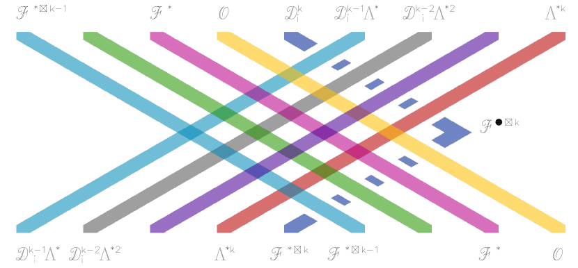
Figure 9. A fleeting glimpse of the subcategory $\langle\operatorname{\mathcal{F}}^{\bullet\boxtimes k}\rangle$.

Lemma 4.14.

$\operatorname{\mathcal{P}}_{{\operatorname{\mathcal{F}}^{\bullet\boxtimes k}}}$ is fully faithful and there is a mutation

$$\langle{\operatorname{\mathcal{F}}^{*\boxtimes k}},\operatorname{\mathcal{F}}^{*\boxtimes k-1},\ldots,\operatorname{\mathcal{O}}\rangle\to\langle\operatorname{\mathcal{F}}^{*\boxtimes k-1},\ldots,\operatorname{\mathcal{O}},{\operatorname{\mathcal{F}}^{\bullet\boxtimes k}}\rangle.$$

Proof.

We first claim that

(4.16) $$\operatorname{RHom}(\operatorname{\mathcal{P}}_{{\operatorname{\mathcal{F}}^{\bullet\boxtimes k}}}(X),\operatorname{\mathcal{P}}_{{\operatorname{\mathcal{F}}^{*\boxtimes m}}}(Y))=0$$

for $X\in D^{b}(\operatorname{Sym}^{k}C)$, $Y\in D^{b}(\operatorname{Sym}^{m}C)$, $m<k$. By (4.15), it suffices to show $\operatorname{RHom}(\operatorname{\mathcal{P}}_{\operatorname{\mathcal{D}}_{i}^{l}{\operatorname{{\boldsymbol{\Lambda}}}^{*}}^{k-l}}(X),\operatorname{\mathcal{P}}_{{\operatorname{\mathcal{F}}^{*\boxtimes m}}}(Y))=0$ for $l\leq k$. By Serre duality, it suffices to prove that $R\Gamma(M_{i},\operatorname{\mathcal{P}}_{\operatorname{\mathcal{D}}_{i}^{l}{\operatorname{{\boldsymbol{\Lambda}}}^{*}}^{k-l}}(X)\otimes^{L}(\operatorname{\mathcal{P}}_{{\operatorname{\mathcal{F}}^{*\boxtimes{m}}}}(Y))^{*}\otimes\omega_{M_{i}})=0$. Without loss of generality, we take $X$ and $Y$ to be skyscraper sheaves. Then $R\Gamma_{M_{i}}(\operatorname{\mathcal{O}}_{M_{i-l}(\Lambda(-2D))}\otimes{\operatorname{{\boldsymbol{\Lambda}}}^{*}}^{k-l}(\operatorname{\mathcal{F}}^{*\boxtimes m}_{D^{\prime}})^{*}\omega_{M_{i}})=R\Gamma_{M_{i-l}(\Lambda(-2D))}({\operatorname{{\boldsymbol{\Lambda}}}^{*}}^{k-l}\bar{\operatorname{\mathcal{F}}}^{\boxtimes m}_{D^{\prime}}\otimes\omega_{M_{i-l}(\Lambda(-2D))}\otimes{\operatorname{{\boldsymbol{\Lambda}}}^{*}}^{l})=R\Gamma(M_{i-l}(\Lambda(-2D)),{\operatorname{{\boldsymbol{\Lambda}}}}^{k}\otimes\bar{\operatorname{\mathcal{F}}}^{\boxtimes m*}_{D^{\prime}})^{*}[\ldots]=0$ by Theorem 3.9 with $j=i-l$, $d=2g-1-2l$, $t=k$, $a=m$, $b=0$ (we have $2g-1-2l>2$ if $l<i$, and $m<k\leq i<2g-3-2i$).

The formula (4.16) follows. Combining with Lemma 4.1 and (4.14), it follows that $\operatorname{RHom}(\operatorname{\mathcal{P}}_{{\operatorname{\mathcal{F}}^{\bullet\boxtimes k}}}(X),\operatorname{\mathcal{P}}_{{\operatorname{\mathcal{F}}^{\bullet\boxtimes k}}}(Y))=\operatorname{RHom}(\operatorname{\mathcal{P}}_{{\operatorname{\mathcal{F}}^{\bullet\boxtimes k}}}(X),\operatorname{\mathcal{P}}_{{\operatorname{\mathcal{F}}^{*\boxtimes k}}}(Y)[k])=\operatorname{RHom}(\operatorname{\mathcal{P}}_{{\operatorname{\mathcal{F}}^{*\boxtimes k}}}(X),\operatorname{\mathcal{P}}_{{\operatorname{\mathcal{F}}^{*\boxtimes k}}}(Y))=\operatorname{RHom}(X,Y)$ by Lemma 4.1, which shows that $\operatorname{\mathcal{P}}_{{\operatorname{\mathcal{F}}^{*\boxtimes k}}}$ is fully faithful and we have a required mutation. ∎

Lemma 4.15.

$\operatorname{\mathcal{P}}_{\operatorname{\mathcal{D}}_{i}^{k}}$ is fully faithful. There is a mutation

$$\langle\operatorname{\mathcal{D}}_{i}^{k-1}\otimes\operatorname{{\boldsymbol{\Lambda}}}^{*},\ldots,{\operatorname{{\boldsymbol{\Lambda}}}^{*}}^{k},\operatorname{\mathcal{F}}^{\bullet\boxtimes k}\rangle\to\langle\operatorname{\mathcal{D}}_{i}^{k},\operatorname{\mathcal{D}}_{i}^{k-1}\otimes\operatorname{{\boldsymbol{\Lambda}}}^{*},\ldots,{\operatorname{{\boldsymbol{\Lambda}}}^{*}}^{k}\rangle.$$

Proof.

We first claim that

(4.17) $$\operatorname{RHom}(\operatorname{\mathcal{P}}_{{\operatorname{\mathcal{F}}^{\bullet\boxtimes k}}}(X),\operatorname{\mathcal{P}}_{\operatorname{\mathcal{D}}_{i}^{l}\otimes{\operatorname{{\boldsymbol{\Lambda}}}^{*}}^{k-l}}(Y))=0$$

for all $X\in D^{b}(\operatorname{Sym}^{k}C)$, $Y\in D^{b}(\operatorname{Sym}^{l}C)$, $l<k$. By (4.14), it suffices to prove that $\operatorname{RHom}(\operatorname{\mathcal{P}}_{{\operatorname{\mathcal{F}}^{*\boxtimes m}}}(X),\operatorname{\mathcal{P}}_{\operatorname{\mathcal{D}}_{i}^{l}\otimes{\operatorname{{\boldsymbol{\Lambda}}}^{*}}^{k-l}}(Y))=0$ for $m\leq k$. Without loss of generality, we take $X$ and $Y$ to be skyscraper sheaves. Then $\operatorname{RHom}({{\operatorname{\mathcal{F}}_{D}^{*\boxtimes m}},\operatorname{\mathcal{O}}_{M_{i-l}(\Lambda(-2D^{\prime}))}\otimes{\operatorname{{\boldsymbol{\Lambda}}}^{*}}^{k-l}})=R\Gamma_{M_{i-l}(\Lambda(-2D^{\prime}))}({{(\operatorname{\mathcal{F}}_{D}^{*\boxtimes m})^{*}}{\operatorname{{\boldsymbol{\Lambda}}}}^{l-k}})=R\Gamma_{M_{i-l}(\Lambda(-2D^{\prime}))}({{\bar{\operatorname{\mathcal{F}}}_{D}^{\boxtimes m}}{\operatorname{{\boldsymbol{\Lambda}}}}^{l-k}})=0$ by Theorem 3.8 with $j=i-l$, $d=2g-1-2l$, $t=l+m-k$, $a=m$, $b=0$ (since $0<l<k\leq i\leq g-1$, we have $1\leq i-l\leq g-1$ and $2<2g-1-2l\leq 2g+1$; also, $m-(i-l)-1<l+m-k<i<2g-3-2i$ and $l+m-k>m$). In addition to (4.17), we have

(4.18) $$\operatorname{RHom}(\operatorname{\mathcal{P}}_{\operatorname{\mathcal{D}}_{i}^{l}\otimes{\operatorname{{\boldsymbol{\Lambda}}}^{*}}^{k-l}}(X),\operatorname{\mathcal{P}}_{\operatorname{\mathcal{D}}_{i}^{k}}(Y))=0$$

for $X\in D^{b}(\operatorname{Sym}^{l}C)$, $Y\in D^{b}(\operatorname{Sym}^{k}C)$, $l<k$. Indeed, by inductive assumption in Theorem 3.2, it suffices to check instead that, for $l<k$, $l+m\leq k$, $m>0$, we have $\operatorname{RHom}(\operatorname{\mathcal{P}}_{{\operatorname{\mathcal{F}}^{*\boxtimes l}}\otimes{\operatorname{{\boldsymbol{\Lambda}}}^{*}}^{m}}(X),\operatorname{\mathcal{P}}_{\operatorname{\mathcal{D}}_{i}^{k}}(Y))=0$. Without loss of generality, we take $X$ and $Y$ to be skyscraper sheaves. Then we compute $\operatorname{RHom}({\operatorname{\mathcal{F}}_{D}^{*\boxtimes l}}\otimes{\operatorname{{\boldsymbol{\Lambda}}}^{*}}^{m},\operatorname{\mathcal{O}}_{M_{i-k}(\Lambda(-2D^{\prime}))})=R\Gamma(M_{i-k}(\Lambda(-2D^{\prime})),{(\operatorname{\mathcal{F}}_{D}^{*\boxtimes l})^{*}}\otimes{\operatorname{{\boldsymbol{\Lambda}}}}^{m})=R\Gamma_{M_{i-k}(\Lambda(-2D^{\prime}))}({{\bar{\operatorname{\mathcal{F}}}_{D}^{\boxtimes l}}{\operatorname{{\boldsymbol{\Lambda}}}}^{m}})=0$ by Theorem 3.9 with $j=i-k$, $d=2g-1-2k$, $t=m$, $a=0$, $b=l$ (we have $d>2$ if $j>0$, and $0<m\leq i<3g-2-2i$).

Combining (4.15), (4.17), (4.18), we see that $\operatorname{RHom}(\operatorname{\mathcal{P}}_{\operatorname{\mathcal{D}}_{i}^{k}}(X),\operatorname{\mathcal{P}}_{\operatorname{\mathcal{D}}_{i}^{k}}(Y))\simeq\operatorname{RHom}(\operatorname{\mathcal{P}}_{{\operatorname{\mathcal{F}}^{\bullet\boxtimes k}}}(X({B\over 2})),\operatorname{\mathcal{P}}_{\operatorname{\mathcal{D}}_{i}^{k}}(Y))\simeq\operatorname{RHom}(\operatorname{\mathcal{P}}_{{\operatorname{\mathcal{F}}^{\bullet\boxtimes k}}}(X({B\over 2})),\operatorname{\mathcal{P}}_{{\operatorname{\mathcal{F}}^{\bullet\boxtimes k}}}(Y({B\over 2})))\simeq\operatorname{RHom}(X({B\over 2}),Y({B\over 2}))$ for $X,Y\in D^{b}(\operatorname{Sym}^{k}C)$ by Lemma 4.14. But the latter group is isomorphic to $\operatorname{RHom}(X,Y)$. This proves the lemma. ∎

Proof of Theorem 3.2.

Part (a) is a part of Lemma 4.15, Part (b) follows from part (c) and induction. Indeed, we can perform the basic Cross Warp mutation Theorem 3.2 (c) in $D^{b}(M_{i-1})$. By inductive assumption and [TT, Section 3], the resulting admissible subcategory maps into itself in $D^{b}(M_{i})$ by the windows embedding $\iota$. It remains to perform the inverse of the basic Cross Warp mutation Theorem 3.2 (c) in $D^{b}(M_{i})$.

Finally, part (c) is a combination of Lemmas 4.1, 4.14, 4.15, and inductive assumption, as illustrated in Figure 9. ∎

5. Broken Loom

In this section we perform a transition from the semi-orthogonal decompositions of $M=M_{g-1}$ with three mega-blocks associated with the birational contraction $\psi:\,M\dashrightarrow\operatorname{{\mathbb{P}}}^{3g-3}$ studied in the previous sections to decompositions with four mega-blocks associated with the birational contraction $\zeta:\,M\to N$. Recall that this morphism is the forgetful map $(F,s)\mapsto F$.

Lemma 5.1.

$D^{b}(M)$ has a semi-orthogonal decomposition into admissible subcategories arranged into three mega-blocks, as follows:

$$\Bigl{\langle}\bigl{\langle}Z^{3+j+2k-g}{\theta^{*}}^{k+j+1}{\operatorname{\mathcal{E}}^{\boxtimes j}}\bigr{\rangle}_{j+k\leq g-2\atop j,k\geq 0},\qquad\qquad\qquad\qquad\qquad$$

(5.1) $$\bigl{\langle}Z^{2+j+2k-g}{\theta^{*}}^{k+j}{\operatorname{\mathcal{E}}^{\boxtimes j}}\bigr{\rangle}_{j+k\leq g-2\atop j,k\geq 0},\$$

$$\qquad\qquad\qquad\qquad\qquad\bigl{\langle}Z^{1+j+2k-g}{\theta^{*}}^{k+j-1}{\operatorname{\mathcal{E}}^{\boxtimes j}}\bigr{\rangle}_{j+k\leq g-1\atop j,k\geq 0}\Bigr{\rangle}.$$

Within each of the three mega-blocks, the blocks are arranged first by $k$ (in the decreasing order) and then, for a fixed $k$, by $j$ (in the decreasing order).

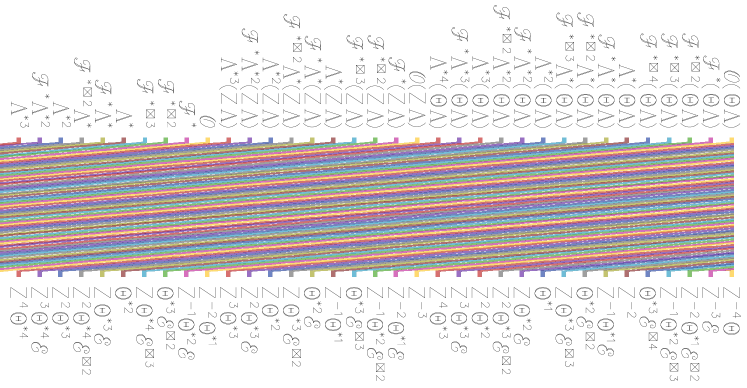
Figure 10. Repeated helix mutation in genus $5$

Proof.

We tensor the semi-orthogonal decomposition of Theorem 3.1 with the line bundle $\omega_{M}^{3-g}=Z^{g-3}\theta^{g-3}\operatorname{{\boldsymbol{\Lambda}}}^{g-3}$, which corresponds to the full rotation of the helix mutation repeated $g-3$ times, see Figure 10 for $g=5$.

We use the formulas $\operatorname{\mathcal{F}}^{*\boxtimes j}\simeq\operatorname{\mathcal{F}}^{\boxtimes j}\otimes(\Lambda^{*\boxtimes j}\boxtimes\operatorname{{\boldsymbol{\Lambda}}}^{*j})\simeq\operatorname{\mathcal{E}}^{\boxtimes j}\otimes(\Lambda^{*\boxtimes j}\boxtimes Z^{-j}\operatorname{{\boldsymbol{\Lambda}}}^{*j})$ to rewrite the decomposition using Fourier–Mukai functors associated with tensor bundles of $\operatorname{\mathcal{E}}$ rather than $\operatorname{\mathcal{F}}$. We use the formula $\operatorname{{\boldsymbol{\Lambda}}}=\theta Z^{-2}$ to eliminate $\operatorname{{\boldsymbol{\Lambda}}}$. Finally, we twist with the line bundle ${\theta^{*}}^{2g-5}$. ∎

Remark 5.2.

The twist by the line bundle $\omega_{M}^{3-g}$ is required to create blocks of the semi-orthogonal decomposition compatible with the contraction $\zeta$. In contrast, the twist by the line bundle ${\theta^{*}}^{2g-5}$, which is pulled back from $N$, is not necessary and we only do it to simplify the formulas. In the illustrations of the braid, we ignore this twist even though we still use it to label the blocks, for consistency.

The next step is crucial. As it turns out, the blocks within each mega-block of (5.1) can be reordered differently. This is illustrated in Figure 11.

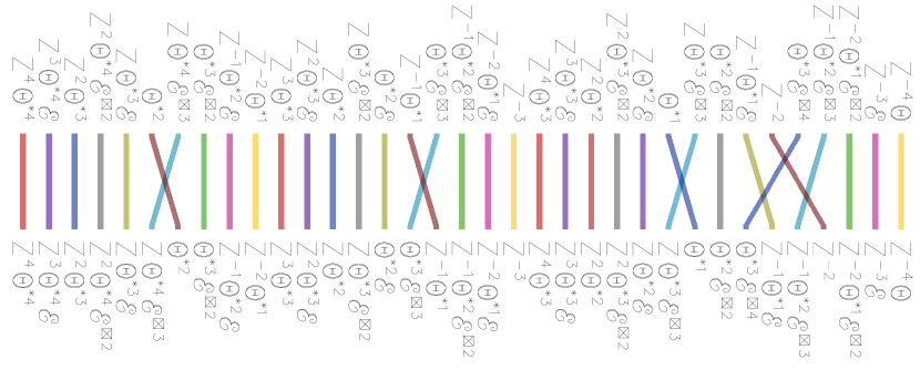
Figure 11. Reordering of the blocks in genus $5$

Theorem 5.3.

$D^{b}(M)$ has a semi-orthogonal decomposition into admissible subcategories arranged into three mega-blocks, as follows:

$$\Bigl{\langle}\bigl{\langle}Z^{3+\lambda-g}{\theta^{*}}^{\lambda-k+1}{\operatorname{\mathcal{E}}^{\boxtimes\lambda-2k}}\bigr{\rangle}_{\lambda-k\leq g-2\atop\lambda-2k,k\geq 0},\qquad\qquad\qquad\qquad\qquad$$

(5.2) $$\bigl{\langle}Z^{2+\lambda-g}{\theta^{*}}^{\lambda-k}{\operatorname{\mathcal{E}}^{\boxtimes\lambda-2k}}\bigr{\rangle}_{\lambda-k\leq g-2\atop\lambda-2k,k\geq 0},\$$

$$\qquad\qquad\qquad\qquad\qquad\bigl{\langle}Z^{1+\lambda-g}{\theta^{*}}^{\lambda-k-1}{\operatorname{\mathcal{E}}^{\boxtimes\lambda-2k}}\bigr{\rangle}_{\lambda-k\leq g-1\atop\lambda-2k,k\geq 0}\Bigr{\rangle}.$$

Within each of the three mega-blocks, the blocks are arranged in decreasing order of $\lambda$. Blocks with the same $\lambda$ are arranged in decreasing order of $k$.

We start with a lemma.

Lemma 5.4.

Suppose $2<d\leq 2g+1$ and $1\leq j\leq\lfloor{d-1\over 2}\rfloor$. Let $D\in\operatorname{Sym}^{a}C$ and $D^{\prime}\in\operatorname{Sym}^{b}C$ with $a,\ b\leq\min(d+g-2j-1,j)$, and let $t$ be an integer satisfying

$$a-j-1<t<d+g-2j-1-b.$$

Suppose, further, that $2t<a-b$. Then

(5.3) $$R\Gamma_{M_{j}(d)}({\operatorname{\mathcal{F}}^{\boxtimes a}_{D}}^{*}\otimes\operatorname{\mathcal{F}}^{\boxtimes b}_{D^{\prime}}\otimes\operatorname{{\boldsymbol{\Lambda}}}^{t})=0$$

Proof.

We write $D=\sum\alpha_{i}x_{i}$ and $D^{\prime}=\sum\beta_{i}y_{i}$, where $\sum\alpha_{i}=a$, $\sum\beta_{i}=b$, and $x_{i}\neq x_{j}$, $y_{i}\neq y_{j}$ for $i\neq j$. It suffices to prove that, under the assumptions of the Lemma,

(5.4) $$R\Gamma_{M_{j}(d)}\left(\bigotimes_{i}{\operatorname{\mathcal{F}}^{*}_{x_{i}}}^{\otimes\alpha_{i}}\otimes\bigotimes_{i}\operatorname{\mathcal{F}}_{y_{i}}^{\otimes\beta_{i}}\otimes\operatorname{{\boldsymbol{\Lambda}}}^{t}\right)=0.$$

Indeed, (5.4) implies (5.3) (see also Remark 5.7) since vector bundles in (5.3) are deformations of vector bundles in (5.4) over $\operatorname{{\mathbb{A}}}^{1}$ by [TT, Corollary 2.9].

Claim 5.5.

It suffices to prove that, under the assumptions of the Lemma,

(5.5) $$R\Gamma_{M_{j}(d)}\left(\bigotimes_{i}\operatorname{Sym}^{\alpha_{i}}{\operatorname{\mathcal{F}}^{*}_{x_{i}}}\otimes\bigotimes_{i}\operatorname{Sym}^{\beta_{i}}\operatorname{\mathcal{F}}_{y_{i}}\otimes\operatorname{{\boldsymbol{\Lambda}}}^{t}\right)=0.$$

Indeed, for every $i$, we have a direct sum decomposition,

(5.6) $$\operatorname{\mathcal{F}}_{y_{i}}^{\otimes\beta_{i}}=\operatorname{Sym}^{\beta_{i}}\operatorname{\mathcal{F}}_{y_{i}}\oplus[\operatorname{{\boldsymbol{\Lambda}}}\otimes\operatorname{Sym}^{\beta_{i}-2}\operatorname{\mathcal{F}}_{y_{i}}]^{\oplus\ldots}\oplus[\operatorname{{\boldsymbol{\Lambda}}}^{2}\otimes\operatorname{Sym}^{\beta_{i}-4}\operatorname{\mathcal{F}}_{y_{i}}]^{\oplus\ldots}\oplus\ldots,$$

which is valid for any rank $2$ vector bundle on any scheme, where the number of copies of each summand is not important for us. We also have the same decompositions for $\operatorname{\mathcal{F}}_{x_{i}}^{\otimes\alpha_{i}}$. Tensored together, these decompositions give a direct sum decomposition of $\bigotimes_{i}{\operatorname{\mathcal{F}}^{*}_{x_{i}}}^{\otimes\alpha_{i}}\otimes\bigotimes_{i}\operatorname{\mathcal{F}}_{y_{i}}^{\otimes\beta_{i}}\otimes\operatorname{{\boldsymbol{\Lambda}}}^{t}$, where all summands have form (5.5) but for different parameters $\alpha_{i}$, $\beta_{i}$, $t$. Concretely, we have to change $a\to a-2u$, $b\to b-2v$, $t\to t-u+v$ for some $u,v\geq 0$. On the other hand, all inequalities in Lemma 5.4 remain valid under this change of parameters. Therefore, if (5.5) is valid for the range of inequalities in the lemma then (5.4) is valid as well. This proves Claim 5.5.

Furthermore, we can assume, without loss of generality, that $b\geq a$ since otherwise we can swap the bundles: $\bigotimes_{i}\operatorname{Sym}^{\alpha_{i}}{\operatorname{\mathcal{F}}^{*}_{x_{i}}}\otimes\bigotimes_{i}\operatorname{Sym}^{\beta_{i}}\operatorname{\mathcal{F}}_{y_{i}}\otimes\operatorname{{\boldsymbol{\Lambda}}}^{t}\simeq\bigotimes_{i}\operatorname{Sym}^{\alpha_{i}}{\operatorname{\mathcal{F}}_{x_{i}}}\otimes\bigotimes_{i}\operatorname{Sym}^{\beta_{i}}\operatorname{\mathcal{F}}^{*}_{y_{i}}\otimes\operatorname{{\boldsymbol{\Lambda}}}^{t-a+b}$ and inequalities in the statement of the lemma still hold: $2(t-a+b)<b-a$, $b-j-1<t-a+b<d+g-2j-1-a$. Note that if $b\geq a$ then $t<0$ by our assumptions and we have vanishing (3.2) by Theorem 3.8. We will reduce (5.5) (for $b\geq a$) to (3.2).

We prove (5.5) by induction on $a+b$. The base case $a=b=0$ is (3.2) for $a=b=0$. As above, we can assume that $b\geq a$ (and so $t<0$).

Claim 5.6.

We have a short exact sequence

(5.7) $$0\to\bigotimes_{i}\operatorname{Sym}^{\beta_{i}}\operatorname{\mathcal{F}}_{y_{i}}\to\bar{\operatorname{\mathcal{F}}}^{\boxtimes b}_{D^{\prime}}\to Q\to 0.$$

Under the induction assumption, $R\Gamma_{M_{j}(d)}\left(\bigotimes_{i}\operatorname{Sym}^{\alpha_{i}}{\operatorname{\mathcal{F}}^{*}_{x_{i}}}\otimes Q\otimes\operatorname{{\boldsymbol{\Lambda}}}^{t}\right)=0$.

Given the claim, we note that $R\Gamma_{M_{j}(d)}\left(\bigotimes_{i}\operatorname{Sym}^{\alpha_{i}}{\operatorname{\mathcal{F}}^{*}_{x_{i}}}\otimes\bar{\operatorname{\mathcal{F}}}^{\boxtimes b}_{D^{\prime}}\otimes\operatorname{{\boldsymbol{\Lambda}}}^{t}\right)$ vanishes as a direct summand of $R\Gamma_{M_{j}(d)}\left(\bigotimes_{i}{\operatorname{\mathcal{F}}^{*}_{x_{i}}}^{\otimes\alpha_{i}}\otimes\bar{\operatorname{\mathcal{F}}}^{\boxtimes b}_{D^{\prime}}\otimes\operatorname{{\boldsymbol{\Lambda}}}^{t}\right),$ which is equal to $0$ by (3.2). Therefore, (5.5) follows from the claim.

It remains to prove Claim 5.6. We use technique and notation from the proof of [TT, Lemma 7.7]. Let $D_{\beta}=\mathbb{C}[t]/(t^{\beta})$ and $B_{\beta}=\frac{\mathbb{C}[t_{1},\ldots,t_{\beta}]}{(\sigma_{1},\ldots,\sigma_{\beta})}$, where $\sigma_{1},\ldots,\sigma_{\beta}$ are elementary symmetric polynomials. Let $\operatorname{{\mathbb{D}}}_{\beta}=\operatorname{Spec}D_{\beta}$ and $\operatorname{{\mathbb{B}}}_{\beta}=\operatorname{Spec}B_{\beta}$. Write the indexing set $\{1,\ldots,b\}$ as a disjoint union of sets $X_{k}$ of cardinality $\beta_{k}$ for $k=1,\ldots,s$, and denote $B=B_{\beta_{1}}\otimes\ldots\otimes B_{\beta_{s}}$. Let $M=M_{j}(d)$. For every $j\in X_{k}$, we have a commutative diagram [TT, (7.6)]

(5.8)

We have $\bar{\operatorname{\mathcal{F}}}^{\boxtimes b}_{D^{\prime}}=\tau_{*}^{S_{\beta_{1}}\times\ldots\times S_{\beta_{s}}}\left(\bigotimes_{j\in X_{k}}\pi_{j}^{*}\operatorname{\mathcal{F}}_{k}\otimes\operatorname{sgn}\right)$, where $\operatorname{\mathcal{F}}_{k}=q_{k}^{*}{\operatorname{\mathcal{F}}}$.

The vector bundle $\tau_{*}\left(\bigotimes\pi_{j}^{*}\operatorname{\mathcal{F}}_{k}\right)$ has a filtration by vector subbundles $\tau_{*}\left(B_{\geq d}\bigotimes\pi_{j}^{*}\operatorname{\mathcal{F}}_{k}\right)$, where $B_{\geq d}\subset B$ is the ideal of monomials of degree $\geq d$. In particular, $\tau_{*}\left(\bigotimes\pi_{j}^{*}\operatorname{\mathcal{F}}_{k}\right)$ has a vector subbundle $\tau_{*}\left(\Delta_{\beta_{1}}\ldots\Delta_{\beta_{s}}\bigotimes\pi_{j}^{*}\operatorname{\mathcal{F}}_{k}\right)$, where $\Delta_{\beta}\in B_{\beta}$ is the top degree monomial (the Vandermonde determinant). The associated graded bundle is $\bigotimes_{k}\operatorname{\mathcal{F}}_{x_{k}}^{\otimes\beta_{k}}\otimes_{\mathcal{O}_{M}}B$. For example, the subbundle $\tau_{*}\left(\Delta_{\beta_{1}}\ldots\Delta_{\beta_{s}}\bigotimes\pi_{j}^{*}\operatorname{\mathcal{F}}_{k}\right)\subset\tau_{*}\left(\bigotimes\pi_{j}^{*}\operatorname{\mathcal{F}}_{k}\right)$ is isomorphic to $\bigotimes_{k}\operatorname{\mathcal{F}}_{x_{k}}^{\otimes\beta_{k}}$.

The group $S_{\beta_{1}}\times\ldots\times S_{\beta_{s}}$ acts on $\bigotimes_{k}\operatorname{\mathcal{F}}_{x_{k}}^{\otimes\beta_{k}}$ by permuting tensor factors within each subset $X_{k}$. The action on $B$ is by the regular representation. The direct sum decomposition of $\bigotimes_{k}\operatorname{\mathcal{F}}_{x_{k}}^{\otimes\beta_{k}}$ induced by (5.6) is equivariant under $S_{\beta_{1}}\times\ldots\times S_{\beta_{s}}$. By Frobenius reciprocity, the vector bundle $\bigotimes_{i}\operatorname{Sym}^{\beta_{i}}\operatorname{\mathcal{F}}_{y_{i}}$ appears in $\left(\bigotimes_{k}\operatorname{\mathcal{F}}_{x_{k}}^{\otimes\beta_{k}}\otimes_{\mathcal{O}_{M}}B\otimes\operatorname{sgn}\right)^{S_{\beta_{1}}\times\ldots\times S_{\beta_{s}}}$ only once and corresponds to the subbundle $\tau_{*}\left(\Delta_{\beta_{1}}\ldots\Delta_{\beta_{s}}\bigotimes_{i}\operatorname{Sym}^{\beta_{i}}\operatorname{\mathcal{F}}_{y_{i}}\right)\subset\tau_{*}\left(\Delta_{\beta_{1}}\ldots\Delta_{\beta_{s}}\bigotimes\pi_{j}^{*}\operatorname{\mathcal{F}}_{k}\right)\subset\tau_{*}(\bigotimes\pi_{j}^{*}\operatorname{\mathcal{F}}_{k})$. It follows that we have a short exact sequence (5.7), where the quotient bundle $Q$ is a direct summand (of skew-invariants) in the bundle $\tilde{Q}=\tau_{*}\left(\bigotimes\pi_{j}^{*}\operatorname{\mathcal{F}}_{k}\right)/\tau_{*}\left(\Delta_{\beta_{1}}\ldots\Delta_{\beta_{s}}\bigotimes\pi_{j}^{*}\operatorname{\mathcal{F}}_{k}\right)$. By the above, $\tilde{Q}$ has a $(S_{\beta_{1}}\times\ldots\times S_{\beta_{s}})$-equivariant filtration by vector bundles with subquotients given by direct sums of vector bundles of the form $\operatorname{{\boldsymbol{\Lambda}}}^{\sum v_{i}}\bigotimes_{i}\operatorname{Sym}^{\beta_{i}-2v_{i}}\operatorname{\mathcal{F}}_{y_{i}}$ with $\sum v_{i}\geq 0$. Furthermore, vector bundles with $\sum v_{i}=0$ have a trivial component of skew-invariants. It follows that $R\Gamma_{M_{j}(d)}\left(\bigotimes_{i}\operatorname{Sym}^{\alpha_{i}}{\operatorname{\mathcal{F}}^{*}_{x_{i}}}\otimes Q\otimes\operatorname{{\boldsymbol{\Lambda}}}^{t}\right)=0$ by the induction assumption. ∎

Remark 5.7.

The proof of Lemma 5.4 also shows that (5.3) holds with $\operatorname{\mathcal{F}}^{\boxtimes a}_{D}$ replaced with $\bar{\operatorname{\mathcal{F}}}^{\boxtimes a}_{D}$ and with $\operatorname{\mathcal{F}}^{\boxtimes b}_{D^{\prime}}$ replaced with $\bar{\operatorname{\mathcal{F}}}^{\boxtimes b}_{D^{\prime}}$.

Proof of Theorem 5.3.

The mega-blocks are the same as in Lemma 5.1, we just do the change of variables $\lambda=2k+j$. The three mega-blocks differ by line bundle twists, in addition, the last mega-block is larger. So it suffices to prove the statement for the last mega-block. We need to check that, whenever $\lambda_{1}<\lambda_{2}$ or $\lambda_{1}=\lambda_{2},k_{1}<k_{2}$,

$$\operatorname{RHom}(Z^{1+\lambda_{1}-g}{\theta^{*}}^{\lambda_{1}-k_{1}-1}{\operatorname{\mathcal{E}}_{D}^{\boxtimes\lambda_{1}-2k_{1}}},Z^{1+\lambda_{2}-g}{\theta^{*}}^{\lambda_{2}-k_{2}-1}{\operatorname{\mathcal{E}}_{D^{\prime}}^{\boxtimes\lambda_{2}-2k_{2}}})=0$$

for every $D\in\operatorname{Sym}^{\lambda_{1}-2k_{1}}C$, $D^{\prime}\in\operatorname{Sym}^{\lambda_{1}-2k_{1}}C$. This $\operatorname{RHom}$ is equal to $R\Gamma\Bigl{(}\Lambda^{t}\otimes(\operatorname{\mathcal{F}}_{D}^{\boxtimes j_{1}})^{*}\otimes\operatorname{\mathcal{F}}^{\boxtimes j_{2}}_{D^{\prime}}\Bigr{)}$, where $t=(k_{1}+j_{1})-(k_{2}+j_{2})$ and, for $i=1,2$, $j_{i}=\lambda_{i}-2k_{i}$. Suppose first that $\lambda_{1}<\lambda_{2}$. We have $j_{1},j_{2}\leq\min(g,g-1)$, so by Lemma 5.4, it suffices to check two numerical conditions:

(5.9) $$j_{1}-g<t<g-j_{2},$$

(5.10) $$2t<j_{1}-j_{2}.$$

Inequalities (5.9) hold for all blocks within the mega-block because, for $i=1,2$, we have that $j_{i}\leq j_{i}+k_{i}$ and $j_{i}+k_{i}\leq g-1<g$. When $\lambda_{1}<\lambda_{2}$, we have

$$2t=2(\lambda_{1}-\lambda_{2})-2(k_{1}-k_{2})<(\lambda_{1}-\lambda_{2})-2(k_{1}-k_{2})=j_{1}-j_{2},$$

so (5.10) holds. On the other hand, when $\lambda_{1}=\lambda_{2}$ and $k_{1}<k_{2}$, we have

$$t=k_{2}-k_{1}<2(k_{2}-k_{1})=j_{1}-j_{2},$$

so the result follows from Theorem 3.8 (3.2) since

$$\Lambda^{t}\otimes(\operatorname{\mathcal{F}}_{D}^{\boxtimes j_{1}})^{*}\otimes\operatorname{\mathcal{F}}^{\boxtimes j_{2}}_{D^{\prime}}\cong\Lambda^{t+j_{2}-j_{1}}\otimes(\bar{\operatorname{\mathcal{F}}}_{D}^{\boxtimes j_{1}})\otimes{\operatorname{\mathcal{F}}^{*\boxtimes j_{2}}_{D^{\prime}}}$$

by Lemma 3.4. ∎

Finally, we prove the following theorem:

Theorem 5.8.

$D^{b}(M)$ has a semi-orthogonal decomposition with semi-orthogonal blocks arranged into the following four mega-blocks:

$$\bigl{\langle}Z^{\lambda+2-g}{\theta^{*}}^{\lambda-k+1}\operatorname{\mathcal{E}}^{\boxtimes\lambda-2k}\bigr{\rangle}_{0\leq\lambda\leq g-2\atop 0\leq k\leq\lfloor{\lambda\over 2}\rfloor},\bigl{\langle}Z^{\lambda+3-g}{\theta^{*}}^{\lambda-k+1}\operatorname{\mathcal{E}}^{\boxtimes\lambda-2k}\bigr{\rangle}_{0\leq\lambda\leq 2(g-2)\atop 0\leq k\leq\lfloor{\lambda\over 2}\rfloor,\lambda-k\leq g-2},$$

$$\bigl{\langle}Z^{\lambda+2-g}{\theta^{*}}^{\lambda-k}\operatorname{\mathcal{E}}^{\boxtimes\lambda-2k}\bigr{\rangle}\!\!\!{}_{0\leq\lambda\leq 2(g-2)\atop 0\leq k\leq\lfloor{\lambda\over 2}\rfloor,\lambda-k\leq g-2}\!\!\!\!,\bigl{\langle}Z^{\lambda+1-g}{\theta^{*}}^{\lambda-k-1}\operatorname{\mathcal{E}}^{\boxtimes\lambda-2k}\bigr{\rangle}\!\!\!\!{}_{g-1\leq\lambda\leq 2(g-1)\atop 0\leq k\leq\lfloor{\lambda\over 2}\rfloor,\lambda-k\leq g-1}\!\!\!\!.$$

Within each mega-block, the blocks are arranged in decreasing order of $\lambda$ and those with identical $\lambda$ are further arranged by decreasing $k$.

Proof.

We split the last mega-block of the semi-orthogonal decomposition of Theorem 5.3 in half: we keep the blocks with $g-1\leq\lambda\leq 2(g-1)$ and tensor the blocks with $0\leq\lambda\leq g-2$ by $\omega_{M}=Z\otimes\theta^{-2}$, which corresponds to mutating them in front of the decomposition as in Figure 12. ∎

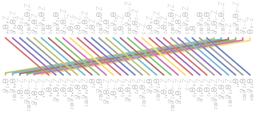
Figure 12. Creation of the fourth mega-block in genus $5$

6. Plain Weave

In the last section we prove Theorem 1.1. We start with the semi-orthogonal decomposition of Theorem 5.8 and observe that the blocks with the trivial power of $Z$ (they correspond to $\lambda=g-2$, $g-3$, $g-2$, and $g-1$ for mega-blocks I, II, III, and IV, respectively,) are pulled-back from the semi-orthogonal blocks of $D^{b}(N)$ of Theorem 1.1. The Plain Weave pattern, illustrated in Figure 13, moves the remaining blocks out of the way.

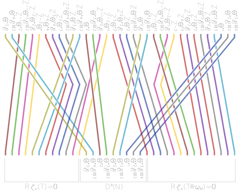
Figure 13. Plain Weave in genus $5$

Notation 6.1.

In view of the semi-orthogonal decomposition

$$D^{b}(M)=\langle\operatorname{\mathcal{A}},\ L\zeta^{*}D^{b}(N)\rangle,\quad\hbox{\rm where}\ \operatorname{\mathcal{A}}=\{T\ :\ R\zeta_{*}(T)=0\}\subset D^{b}(M),$$

it suffices to prove that the blocks from Theorem 5.8 that are not pulled back from $N$ can be mutated into the subcategory $\operatorname{\mathcal{A}}$. To preserve symmetry, we actually mutate some of the blocks that are not pulled back from $N$ to the left of the subcategory generated by the pulled back blocks, and prove that they go into the subcategory $\operatorname{\mathcal{A}}$, and mutate the remaining blocks that are not pulled back from $N$ to the right of the subcategory generated by the pulled back blocks, and prove that they end up in the subcategory $\operatorname{\mathcal{A}}^{\prime}=\{T\ :\ R\zeta_{*}(T\otimes\omega_{M})=0\}$. This is illustrated in Figure 13. Once this is done, we can tensor the blocks contained in $\operatorname{\mathcal{A}}^{\prime}$ with $\omega_{M}$, which mutates them to the left of the semi-orthogonal decomposition and into the subcategory  $\operatorname{\mathcal{A}}$. This will prove Theorem 1.1.

Remark 6.2.

In contrast to the previous sections of the paper, we don’t have to study the kernels of the Fourier–Mukai functors that embed the left-over blocks into the subcategory $\operatorname{\mathcal{A}}$. By the main result of [kosekitoda], the category $\operatorname{\mathcal{A}}$ is isomorphic to the derived category of the moduli space of stable pairs with fixed determinant $K_{C}\otimes\Lambda^{*}$ of degree $2g-3$. The latter category has a semi-orthogonal decomposition obtained using the tower of flips similar to Theorem 2.2. There likely exists a mutation that connects blocks of this semi-orthogonal decomposition to our left-over blocks in $D^{b}(M)$.

We need the following theorem, proved later in this section. Recall that $\operatorname{\mathcal{D}}^{l}$ is the structure sheaf of $D^{l}=\{(D,F,s):\,s|_{D}=0\}\subset\operatorname{Sym}^{l}C\times M$.

Theorem 6.3.

Let $0\leq 2l\leq k\leq g-1$. Let $\Phi:\,D^{b}(M)\to{}^{\perp}\langle\operatorname{\mathcal{E}}^{\boxtimes k}\rangle$ be the projection functor. Then $\Phi(Z^{k}\otimes\langle(\operatorname{\mathcal{D}}^{l})^{\vee}\rangle)\subset\operatorname{\mathcal{A}}^{\prime}$.

We will first finish the proof of Theorem 1.1.

Proof of Theorem 1.1.

We process blocks of the semi-orthogonal decomposition of Theorem 5.8, mega-block by mega-block. We also split mega-blocks II and III into half-mega-blocks, II=IIa+IIb and III=IIIa+IIIb. Recall that, within each mega-block, the blocks are arranged by $\lambda$ in the decreasing order. The reader may wish to inspect Figure 13 as we go along.

On the right side of Figure 13, Mega-block IV contains the blocks

(6.1) $$\bigl{\langle}Z^{\lambda+1-g}{\theta^{*}}^{\lambda-m-1}\operatorname{\mathcal{E}}^{\boxtimes\lambda-2m}\bigr{\rangle}_{g-1\leq\lambda\leq 2(g-1)\atop 0\leq m\leq\lfloor{\lambda\over 2}\rfloor,\lambda-m\leq g-1}$$

and ends with the blocks with $\lambda=g-1$,

(6.2) $$\bigl{\langle}{\theta^{*}}^{(g-1)-k-1}\operatorname{\mathcal{E}}^{\boxtimes(g-1)-2k}\bigr{\rangle}_{0\leq k\leq\lfloor{g-1\over 2}\rfloor},$$

which are pulled back from $N$ and are ordered by $k$, in decreasing order. We process the remaining blocks in the increasing order of $\lambda$. Take one of the blocks $\operatorname{\mathcal{C}}$ from (6.1) with $\lambda\geq g$. We will take some blocks (one or two) from (6.2), temporarily move them in front of all other blocks in (6.2), and call the subcategory generated by them $\operatorname{\mathcal{B}}$. Some of the remaining blocks in (6.1) will mutate in the process but will remain in the subcategory pulled back from $N$. We then mutate the block $\operatorname{\mathcal{C}}$ to the right of $\operatorname{\mathcal{B}}$ (into the subcategory ${}^{\perp}\operatorname{\mathcal{B}}$) and show that the mutated block $\operatorname{\mathcal{C}}^{\prime}$ is contained in the subcategory $\operatorname{\mathcal{A}}^{\prime}$. Therefore, the mutated block $\operatorname{\mathcal{C}}^{\prime}$ becomes orthogonal to the remaining blocks in (6.2), some of them mutated, since all of them are pulled back from $N$. So we can move the mutated block $\operatorname{\mathcal{C}}^{\prime}$, unchanged, to the right of all the blocks in (6.2). Finally, we move the blocks from $\operatorname{\mathcal{B}}$ back into their position in the sequence (6.2). To realize this program, we need the following lemma:

Lemma 6.4.

Suppose $g\leq\lambda\leq 2(g-1)$, $0\leq m\leq\lfloor{\lambda\over 2}\rfloor$, and $\lambda-m\leq g-1$. The orthogonal projector onto ${}^{\perp}\operatorname{\mathcal{B}}$ takes the block $\bigl{\langle}Z^{\lambda+1-g}{\theta^{*}}^{\lambda-m-1}\operatorname{\mathcal{E}}^{\boxtimes\lambda-2m}\bigr{\rangle}$ into $\operatorname{\mathcal{A}}^{\prime}$, where $\operatorname{\mathcal{B}}$ is given by two blocks from (6.2), namely one block with $k=g-1-\lambda+m$ and another with $k=g-\lambda+m$, unless $\lambda=2m$, in which case we take only one block, namely the block with $k=g-1-\lambda+m$.

Proof.

We rewrite the kernel vector bundle as

$$Z^{\lambda+1-g}{\theta^{*}}^{\lambda-m-1}\operatorname{\mathcal{E}}^{\boxtimes\lambda-2m}\simeq Z^{2m+1-g}{\theta^{*}}^{m-1}\operatorname{\mathcal{F}}^{*\boxtimes\lambda-2m}.$$

Take the complex $Z^{2m+1-g}{\theta^{*}}^{m-1}\operatorname{\mathcal{F}}^{\bullet\lambda-2m}$ from Definition 4.6. If $\lambda\neq 2m$, let $Z^{2m+1-g}{\theta^{*}}^{m-1}\otimes[\operatorname{\mathcal{F}}^{*\boxtimes\lambda-2m}\to\operatorname{Ker}^{1-(\lambda-2m)}]$ be its $2$-step smart truncation. By Lemma 4.9 and Corollary 4.10, it suffices to prove that the subcategory $\langle Z^{2m+1-g}{\theta^{*}}^{m-1}\operatorname{{\boldsymbol{\Lambda}}}^{*\lambda-2m}\rangle$, and subcategories $\langle Z^{2m+1-g}{\theta^{*}}^{m-1}\operatorname{{\boldsymbol{\Lambda}}}^{*\lambda-2m-1}\rangle$ and $\langle Z^{2m+1-g}{\theta^{*}}^{m-1}\operatorname{{\boldsymbol{\Lambda}}}^{*\lambda-2m}[\operatorname{\mathcal{D}}^{1}]^{\vee}\rangle$, which are necessary only if $\lambda\neq 2m$, are moved into $\operatorname{\mathcal{A}}^{\prime}$ by the projector onto ${}^{\perp}\operatorname{\mathcal{B}}$ from the lemma. But these subcategories are the same as $\langle Z^{1-g+2\lambda-2m}{\theta^{*}}^{\lambda-m-1}\rangle$, $\langle Z^{-1-g+2\lambda-2m}{\theta^{*}}^{\lambda-m-2}\rangle$, and $\langle Z^{1-g+2\lambda-2m}{\theta^{*}}^{\lambda-m-1}[\operatorname{\mathcal{D}}^{1}]^{\vee}\rangle$, so the claim follows from Theorem 6.3.

We only need to check that the block with $k=g-1-\lambda+m$ (and also with $k=g-\lambda+m$ if $\lambda\neq 2m$) is among the blocks in (6.2), i.e. that $0\leq k\leq\lfloor{g-1\over 2}\rfloor$. The first inequality follows from the inequality $\lambda-m\leq g-1$. To show that $g-\lambda+m\leq\lfloor{g-1\over 2}\rfloor$, or equivalently that $\lambda-m\geq\lceil{g+1\over 2}\rceil$ we use that $\lambda-m\geq\lambda-\lfloor{\lambda\over 2}\rfloor=\lceil{\lambda\over 2}\rceil\geq\lceil{g\over 2}\rceil$. This shows that $\lambda-m\geq\lceil{g+1\over 2}\rceil$ unless $\lambda=2m$, in which case a weaker inequality $\lambda-m\geq\lceil{g-1\over 2}\rceil$ still holds. ∎

At the end of the process, the blocks from (6.2) move to the left side of the mega-block IV unchanged and all other blocks from (6.1) mutate to the right side and into the subcategory $\operatorname{\mathcal{A}}^{\prime}$.

On the left side of Figure 13, Mega-block I contains the blocks

(6.3) $$\bigl{\langle}Z^{\lambda-(g-2)}{\theta^{*}}^{\lambda-m+1}\operatorname{\mathcal{E}}^{\boxtimes\lambda-2m}\bigr{\rangle}_{0\leq\lambda\leq g-2\atop 0\leq m\leq\lfloor{\lambda\over 2}\rfloor}$$

and starts with the blocks with $\lambda=g-2$,

(6.4) $$\bigl{\langle}{\theta^{*}}^{(g-2)-k+1}\operatorname{\mathcal{E}}^{\boxtimes(g-2)-2k}\bigr{\rangle}_{0\leq k\leq\lfloor{g-2\over 2}\rfloor},$$

which are pulled back from $N$ and are ordered by decreasing $k$. We process the remaining blocks in (6.3) inductively, in the decreasing order of $\lambda$. The processed blocks will mutate to the left of the blocks (6.4) and into the subcategory $\operatorname{\mathcal{A}}$. Equivalently, we can mutate the blocks dual to (6.3),

(6.5) $$\bigl{\langle}Z^{-\lambda+(g-2)}{\theta^{*}}^{-m-1}\operatorname{\mathcal{E}}^{\boxtimes\lambda-2m}\bigr{\rangle}_{0\leq\lambda\leq g-2\atop 0\leq m\leq\lfloor{\lambda\over 2}\rfloor},$$

into $\operatorname{\mathcal{A}}^{\prime}$ under the blocks dual to (6.4), namely

(6.6) $$\bigl{\langle}{\theta^{*}}^{-k-1}\operatorname{\mathcal{E}}^{\boxtimes(g-2)-2k}\bigr{\rangle}_{0\leq k\leq\lfloor{g-2\over 2}\rfloor}.$$

Take the next block to process from (6.5). Arguing as in the case of mega-block IV, it suffices to prove the following lemma:

Lemma 6.5.

Suppose $0\leq\lambda\leq g-2$, $0\leq m\leq\lfloor{\lambda\over 2}\rfloor$. The orthogonal projector onto ${}^{\perp}\operatorname{\mathcal{B}}$ takes the block $\bigl{\langle}Z^{-\lambda+(g-2)}{\theta^{*}}^{-m-1}\operatorname{\mathcal{E}}^{\boxtimes\lambda-2m}\bigr{\rangle}$ into $\operatorname{\mathcal{A}}^{\prime}$, where $\operatorname{\mathcal{B}}$ is given by two blocks from (6.4) with $k=m$ and $m+1$, unless $\lambda=2m$, in which case we take only one block, namely the block with $k=m$.

Proof.

We rewrite the kernel vector bundle as

$$Z^{-\lambda+(g-2)}{\theta^{*}}^{-m-1}\operatorname{\mathcal{E}}^{\boxtimes\lambda-2m}\simeq Z^{(g-2)+2m-2\lambda}{\theta^{*}}^{-\lambda+m-1}\operatorname{\mathcal{F}}^{*\boxtimes\lambda-2m}.$$

Take the complex $Z^{(g-2)+2m-2\lambda}{\theta^{*}}^{-\lambda+m-1}\operatorname{\mathcal{F}}^{\bullet\lambda-2m}$ from Definition 4.6.If $\lambda\neq 2m$, let $Z^{(g-2)+2m-2\lambda}{\theta^{*}}^{-\lambda+m-1}\otimes[\operatorname{\mathcal{F}}^{*\boxtimes\lambda-2m}\to\operatorname{Ker}^{1-(\lambda-2m)}]$ be its $2$-step smart truncation. By Lemma 4.9 and Corollary 4.10, it suffices to prove that the subcategory $\langle Z^{(g-2)+2m-2\lambda}{\theta^{*}}^{-\lambda+m-1}\operatorname{{\boldsymbol{\Lambda}}}^{*\lambda-2m}\rangle$, and subcategories $\langle Z^{(g-2)+2m-2\lambda}{\theta^{*}}^{-\lambda+m-1}\operatorname{{\boldsymbol{\Lambda}}}^{*\lambda-2m-1}\rangle$, $\langle Z^{(g-2)+2m-2\lambda}{\theta^{*}}^{-\lambda+m-1}\operatorname{{\boldsymbol{\Lambda}}}^{*\lambda-2m}[\operatorname{\mathcal{D}}^{1}]^{\vee}\rangle$ if $\lambda\neq 2m$, are moved into $\operatorname{\mathcal{A}}^{\prime}$ by the projector from the lemma. These subcategories are the same as $\langle Z^{(g-2)-2m}{\theta^{*}}^{-m-1}\rangle$, $\langle Z^{(g-2)-2m-2}{\theta^{*}}^{-m-2}\rangle$, $\langle Z^{(g-2)-2m}{\theta^{*}}^{-m-1}[\operatorname{\mathcal{D}}^{1}]^{\vee}\rangle$. So the claim follows from Theorem 6.3. ∎

Mega-block IIa contains the blocks

(6.7) $$\bigl{\langle}Z^{\lambda-(g-3)}{\theta^{*}}^{\lambda-m+1}\operatorname{\mathcal{E}}^{\boxtimes\lambda-2m}\bigr{\rangle}_{g-2\leq\lambda\leq 2(g-2)\atop 0\leq m\leq\lfloor{\lambda\over 2}\rfloor,\lambda-m\leq g-2}$$

and ends with the blocks with $\lambda=g-2$,

(6.8) $$\bigl{\langle}Z{\theta^{*}}^{(g-2)-k+1}\operatorname{\mathcal{E}}^{\boxtimes(g-2)-2k}\bigr{\rangle}_{0\leq k\leq\lfloor{g-2\over 2}\rfloor}.$$

These blocks are not pulled back from $N$ but they are fairly close: they are exactly the same blocks as (6.4) but tensored with $Z$. We start by keeping the blocks (6.8) and processing the remaining blocks in (6.7) inductively, in the increasing order of $\lambda$. As with mega-block IV, for each block $\operatorname{\mathcal{C}}$ from (6.7) we take one or two blocks from (6.8) (call the subcategory they generate $\operatorname{\mathcal{B}}$) and temporarily move them to the left of the other blocks in (6.8); these other blocks may mutate, but they remain in $Z\zeta^{*}(D^{b}(N))$. We then mutate $\operatorname{\mathcal{C}}$ as in mega-block IV, but because of the tensoring with $Z$, $\operatorname{\mathcal{C}}$ will mutate to right of the block $\operatorname{\mathcal{B}}$ and into the subcategory $\operatorname{\mathcal{A}}$ instead of the category $\operatorname{\mathcal{A}}^{\prime}$. The processed block $\operatorname{\mathcal{C}}^{\prime}$ is then orthogonal to other blocks in (6.8) (some mutated) by projection formula and Serre duality. So we can move $\operatorname{\mathcal{C}}^{\prime}$ to the right of all the blocks in (6.8) and to the left of the previously processed blocks from the mega-block IIa. We then return $\operatorname{\mathcal{B}}$ to its position in (6.8) and continue with the next block from (6.7). At the end of the process, the blocks from (6.8) move to the left side of the mega-block IIa and all other blocks from it mutate to the right side of the mega-block IIa and into the subcategory $\operatorname{\mathcal{A}}$.

At this point, the blocks in (6.4) directly precede the blocks in (6.8). We use the standard short exact sequence

$$0\to\operatorname{\mathcal{O}}_{M}\to\operatorname{\mathcal{O}}_{M}(Z)\to\operatorname{\mathcal{O}}_{Z}(Z)\to 0.$$

Let $T={\theta^{*}}^{(g-2)-k+1}\operatorname{\mathcal{E}}^{\boxtimes(g-2)-2k}$. For every $k$ in increasing order, we move the block $\operatorname{\mathcal{B}}=\bigl{\langle}T\bigl{\rangle}$ in (6.4) to the right of the other blocks in (6.4), which may mutate within $\zeta^{*}(D^{b}(N))$. We then mutate the block $\operatorname{\mathcal{C}}=\bigl{\langle}ZT\bigl{\rangle}$ from (6.8) to the left of $\operatorname{\mathcal{B}}$, producing a block $\operatorname{\mathcal{C}}^{\prime}$ embedded by the composition of the Fourier–Mukai functor $\operatorname{\mathcal{P}}_{ZT}$ and derived restriction to $Z$. Since $R\zeta_{*}(\operatorname{\mathcal{O}}_{Z}(Z))=0$ and by projection formula, the block $\operatorname{\mathcal{C}}^{\prime}$ is contained in the subcategory $\operatorname{\mathcal{A}}$, and so orthogonal to the blocks (6.4) (some mutated). So we move $\operatorname{\mathcal{C}}^{\prime}$ to the left of the blocks (6.4) and return $\operatorname{\mathcal{B}}$ to its position, undoing any mutation of (6.4). We continue to mutate all blocks from (6.8) to the left of the blocks in (6.4) and into the subcategory $\operatorname{\mathcal{A}}$. After this mutation, the blocks in (6.4) precede the processed blocks from mega-block IIa with $\lambda>g-2$. These blocks are all contained in the subcategory $\operatorname{\mathcal{A}}$, and so are orthogonal to all blocks in (6.4). So we can move all these blocks to the left of all the blocks in (6.4).

At the end, the blocks from (6.4) move to the right side of both the mega-block I and the mega-block IIa and all other blocks from these mega-blocks mutate to the left side and into the subcategory $\operatorname{\mathcal{A}}$.

Mega-block IIb contains the blocks

$$\bigl{\langle}Z^{\lambda+3-g}{\theta^{*}}^{\lambda-m+1}\operatorname{\mathcal{E}}^{\boxtimes\lambda-2m}\bigr{\rangle}_{0\leq\lambda\leq g-3\atop 0\leq m\leq\lfloor{\lambda\over 2}\rfloor}$$

and starts with the blocks with $\lambda=g-3$,

(6.9) $$\bigl{\langle}{\theta^{*}}^{(g-3)-k+1}\operatorname{\mathcal{E}}^{\boxtimes(g-3)-2k}\bigr{\rangle}_{0\leq k\leq\lfloor{g-3\over 2}\rfloor},$$

which are pulled back from $N$ and are ordered by decreasing $k$. We argue in the same way as for the mega-block I: blocks in (6.9) can be moved to the right, and the remaining blocks of the mega-block mutated to the left and into the subcategory  $\operatorname{\mathcal{A}}$. In particular, they become orthogonal to the blocks in (6.4) by projection formula and can be moved to the left of them.

At this point of our algorithm, the blocks from (6.4) and (6.9) move unchanged to the right of all of the blocks in mega-blocks I and II and all the other blocks in these mega-blocks mutate to the left and into the subcategory $\operatorname{\mathcal{A}}$. Note that Figure 13 contains two connected components and we have finished analysis of the left connected component as well as the mega-block IV from the right connected component. Analysis of the remaining mega-blocks is similar.

Mega-block IIIb contains the blocks

$$\bigl{\langle}Z^{\lambda+2-g}{\theta^{*}}^{\lambda-m}\operatorname{\mathcal{E}}^{\boxtimes\lambda-2m}\bigr{\rangle}_{g-3\leq\lambda\leq 2(g-2)\atop 0\leq m\leq\lfloor{\lambda\over 2}\rfloor,\lambda-m\leq g-2}$$

and starts with the blocks with $\lambda=g-3$,

(6.10) $$\bigl{\langle}Z^{-1}{\theta^{*}}^{(g-3)-k}\operatorname{\mathcal{E}}^{\boxtimes(g-3)-2k}\bigr{\rangle}_{0\leq k\leq\lfloor{(g-3)\over 2}\rfloor}.$$

We argue in the same way as for the mega-block IIb: the blocks in (6.10) can be moved unchanged to the right of the mega-block, and the remaining blocks mutated to the left and into the subcategory $\operatorname{\mathcal{A}}$.

At this point, the blocks in (6.10) precede the blocks in (6.2) (with $k\geq 1$). Let $T={\theta^{*}}^{(g-3)-k}\operatorname{\mathcal{E}}^{\boxtimes(g-3)-2k}$. For every $k$ with $1\leq k\leq\lfloor{(g-3)\over 2}\rfloor$, we pull the block $\operatorname{\mathcal{B}}=\bigl{\langle}T\bigl{\rangle}$ to the left side of (6.2). We use the short exact sequence

$$0\to\operatorname{\mathcal{O}}_{M}(-Z)\to\operatorname{\mathcal{O}}_{M}\to\operatorname{\mathcal{O}}_{Z}\to 0.$$

and mutate the block $\operatorname{\mathcal{C}}=\bigl{\langle}Z^{-1}T\bigl{\rangle}$ to the right of $\operatorname{\mathcal{B}}$, producing the block $\operatorname{\mathcal{C}}^{\prime}$ embedded by the composition of the Fourier–Mukai functor $\operatorname{\mathcal{P}}_{T}$ and the derived restriction to $Z$. Since $R\zeta_{*}(\operatorname{\mathcal{O}}_{Z}(\omega_{M}))=0$, the block $\operatorname{\mathcal{C}}^{\prime}$ is contained in the subcategory $\operatorname{\mathcal{A}}^{\prime}$, and so is orthogonal to all the blocks in (6.2). So we can move $\operatorname{\mathcal{C}}^{\prime}$ to the right of all the blocks in (6.2) and move $\operatorname{\mathcal{B}}$ back into position. At this point, the blocks in (6.2) follow the processed blocks from mega-block IIIb. Since the processed blocks are all contained in the subcategory $\operatorname{\mathcal{A}}^{\prime}$, they are orthogonal to the blocks in (6.2). So we can move all the processed blocks to the right of all the blocks in (6.4). At this point, the blocks from (6.2) are to the left of all the other blocks from mega-blocks IIIb and IV and all other blocks from these mega-blocks mutated to the right side and into the subcategory $\operatorname{\mathcal{A}}^{\prime}$.

Mega-block IIIa contains the blocks

$$\bigl{\langle}Z^{\lambda+2-g}{\theta^{*}}^{\lambda-m}\operatorname{\mathcal{E}}^{\boxtimes\lambda-2m}\bigr{\rangle}_{g-2\leq\lambda\leq 2(g-2)\atop 0\leq m\leq\lfloor{\lambda\over 2}\rfloor,\lambda-m\leq g-2}$$

and ends with the blocks with $\lambda=g-2$,

(6.11) $$\bigl{\langle}{\theta^{*}}^{(g-2)-k}\operatorname{\mathcal{E}}^{\boxtimes(g-2)-2k}\bigr{\rangle}_{0\leq k\leq\lfloor{g-2\over 2}\rfloor},$$

which are pulled back from $N$ and are orthogonal to each other. The analysis of this mega-block is entirely analogous to the mega-block IV: the blocks from (6.11) can be moved to the left side of the mega-block unchanged and the remaining blocks mutated to the right side and into the subcategory $\operatorname{\mathcal{A}}^{\prime}$. After that, they become orthogonal to the blocks in (6.2) and can be moved to the right of all of them.

Our semi-orthogonal decomposition now looks as follows: the blocks (6.4), (6.9), (6.11), and (6.2) pulled back from $N$ are moved unchanged to be together in the middle, the remaining blocks from mega-blocks I and II are mutated to the left and into the subcategory $\operatorname{\mathcal{A}}=\{T\,:\,R\zeta_{*}(T)=0\}$, while the remaining blocks from mega-blocks III and IV are mutated to the right and into the subcategory $\operatorname{\mathcal{A}}^{\prime}=\{T\,:\,R\zeta_{*}(T\otimes\omega_{M})=0\}$. This is illustrated in Figure 13. After that, we can further tensor the blocks in $\{T\,:\,R\zeta_{*}(T\otimes\omega_{M})=0\}$ with $\omega_{M}$, which mutates them to the left of the semi-orthogonal decomposition and into $\{T\,:\,R\zeta_{*}(T)=0\}=D^{b}(N)^{\perp}$. This proves Theorem 1.1. ∎

Next, we are going to prove Theorem 6.3.

Since the projector $\Phi:\,D^{b}(M)\to{}^{\perp}\langle\operatorname{\mathcal{E}}^{\boxtimes k}\rangle$ is a Fourier–Mukai functor given by some object in $D^{b}(M\times M)$, the same is true for the functor

(6.12) $$\operatorname{\mathcal{Z}}^{1}\circ\Phi\circ\operatorname{\mathcal{P}}_{Z^{k}\otimes(\operatorname{\mathcal{D}}^{l})^{\vee}}:\,D^{b}(\operatorname{Sym}^{l}C)\to D^{b}(N),$$

where we let $\operatorname{\mathcal{Z}}^{s}:\,D^{b}(M)\to D^{b}(N)$ be the functor given by $R\zeta_{*}(\bullet\otimes Z^{s}))$. Theorem 6.3 asserts that (6.12) is a $0$ functor, i.e. its kernel is equal to $0$. By Nakayama’s lemma, it suffices to prove that $\operatorname{\mathcal{Z}}^{1}\circ\Phi\circ\operatorname{\mathcal{P}}_{Z^{k}\otimes(\operatorname{\mathcal{D}}^{l})^{\vee}}(\operatorname{\mathcal{O}}_{\{D\}})=0$ for all points $D\in\operatorname{Sym}^{l}C$, where $\operatorname{\mathcal{O}}_{\{D\}}$ is the skyscraper sheaf. Equivalently,

(6.13) $$\operatorname{\mathcal{Z}}^{1}\circ\Phi(Z^{k}\otimes\operatorname{\mathcal{O}}^{\vee}_{M(-D)})=0,$$

where we denote by $M(-D)\subset M$ the locus of stable pairs such that the universal section $\Sigma$ vanishes at $D$.

Notation 6.6.

For a Fourier–Mukai functor $\operatorname{\mathcal{P}}_{K}:\,D^{b}(X)\to D^{b}(Y)$, let $\operatorname{\mathcal{P}}^{*}_{K}$ be its left adjoint functor. It is a Fourier–Mukai functor with the kernel $K^{\vee}\otimes\omega_{Y}^{\bullet}$, where $\omega_{Y}^{\bullet}$ is the dualizing complex and $K^{\vee}$ is the derived dual.

Lemma 6.7.

Consider the diagram

(6.14)

where double arrows are natural transformations of functors. The one in the middle is the unit of adjunction $\operatorname{Id}\to\operatorname{\mathcal{P}}_{\operatorname{\mathcal{E}}^{\boxtimes k}}\circ\operatorname{\mathcal{P}}^{*}_{\operatorname{\mathcal{E}}^{\boxtimes k}}$. Then (6.13) is equivalent to the statement that the following morphism (given by the bottom natural transformation in (6.14)) is an isomorphism:

(6.15) $$\operatorname{\mathcal{Z}}^{1}(Z^{k}\otimes\operatorname{\mathcal{O}}^{\vee}_{M(-D)})\to\operatorname{\mathcal{Z}}^{1}\circ\operatorname{\mathcal{P}}_{\operatorname{\mathcal{E}}^{\boxtimes k}}\circ\operatorname{\mathcal{P}}^{*}_{\operatorname{\mathcal{E}}^{\boxtimes k}}(Z^{k}\otimes\operatorname{\mathcal{O}}^{\vee}_{M(-D)}).$$

Proof.

For an admissible subcategory $\operatorname{\mathcal{B}}\subset D^{b}(X)$, the semi-orthogonal projector $D^{b}(X)\to{}^{\perp}\operatorname{\mathcal{B}}$ is given by the cone (shifted by $-1$) of the unit of adjunction $\operatorname{Id}\to i_{\operatorname{\mathcal{B}}}\circ i^{*}_{\operatorname{\mathcal{B}}}$, where $i_{\operatorname{\mathcal{B}}}$ is the inclusion of $\operatorname{\mathcal{B}}$ and $i^{*}_{\operatorname{\mathcal{B}}}$ is its left adjoint [bondal-orlov]. In our set-up, $\operatorname{\mathcal{B}}=\langle\operatorname{\mathcal{E}}^{\boxtimes k}\rangle$ and (6.13) asserts that the cone becomes zero after tensoring with $Z$ and pushing forward to $N$, which is equivalent to the statement of the lemma. ∎

Next, we compute both sides in (6.15).

Notation 6.8.

Recall that $M(-D)\subset M$ is isomorphic to the moduli space of stable pairs with determinant $\Lambda^{\prime}=\Lambda(-2D)$ of degree $2g-1-2l$.We denote this moduli space by $M^{\prime}$. It is smooth, of dimension $3g-3-2l$. There is a forgetful morphism $\zeta^{\prime}:\,M^{\prime}\to N^{\prime}$, where $N^{\prime}\simeq N$ is the moduli space of rank $2$ vector bundles with determinant $\Lambda^{\prime}$. Let $\operatorname{\mathcal{E}}^{\prime}$ be the universal bundle on $C\times N^{\prime}$. Let $(\operatorname{\mathcal{F}}^{\prime},\Sigma^{\prime})$ be the universal stable pair of $M^{\prime}$. We have

(6.16) $$\operatorname{\mathcal{F}}^{\prime}\simeq\operatorname{\mathcal{F}}(-D)|_{C\times M(-D)}.$$

Lemma 6.9.

In the notation of Lemma 6.7,

$$\operatorname{\mathcal{P}}^{*}_{\operatorname{\mathcal{E}}^{\boxtimes k}}(Z^{k}\otimes\operatorname{\mathcal{O}}^{\vee}_{M(-D)})\simeq\operatorname{\mathcal{O}}(-D)^{\boxtimes k}.$$

Proof.

Indeed, $\operatorname{\mathcal{P}}^{*}_{\operatorname{\mathcal{E}}^{\boxtimes k}}(Z^{k}\otimes\operatorname{\mathcal{O}}^{\vee}_{M(-D)})=R{\pi_{\operatorname{Sym}^{k}C*}}(\operatorname{\mathcal{O}}^{\vee}_{M(-D)}\otimes{\operatorname{\mathcal{F}}^{\boxtimes k}}^{*}\otimes\omega_{M}^{\bullet})\simeq\left[R{\pi_{\operatorname{Sym}^{k}C*}}(\operatorname{\mathcal{F}}^{\boxtimes k}|_{\operatorname{Sym}^{k}C\times M(-D)})\right]^{\vee}\simeq\left[R{\pi_{\operatorname{Sym}^{k}C*}}(\left(\operatorname{\mathcal{F}}^{\prime}(D)\right)^{\boxtimes k})\right]^{\vee}$. By projection formula, this is isomorphic to $\left[R{\pi_{\operatorname{Sym}^{k}C*}}(\operatorname{\mathcal{F}}^{\prime\boxtimes k})\right]^{\vee}\otimes\operatorname{\mathcal{O}}(-D)^{\boxtimes k}$, which in turn is isomorphic to $\operatorname{\mathcal{O}}(-D)^{\boxtimes k}$ by [TT, Proposition 7.2]. ∎

Next, $\operatorname{\mathcal{P}}_{\operatorname{\mathcal{E}}^{\boxtimes k}}(\operatorname{\mathcal{O}}(-D)^{\boxtimes k})=R\pi_{M*}(\operatorname{\mathcal{E}}^{\boxtimes k}\otimes\operatorname{\mathcal{O}}(-D)^{\boxtimes k})\simeq R\pi_{M*}(\operatorname{\mathcal{E}}(-D)^{\boxtimes k})$. The morphism $Z^{k}\otimes\operatorname{\mathcal{O}}^{\vee}_{M(-D)}\to R\pi_{M*}(\operatorname{\mathcal{E}}(-D)^{\boxtimes k})$ given by the middle row in (6.14) is adjoint to a morphism $L\pi_{M}^{*}(Z^{k}\otimes\operatorname{\mathcal{O}}^{\vee}_{M(-D)})\to\operatorname{\mathcal{E}}(-D)^{\boxtimes k}$, which is dual to a morphism $\operatorname{\mathcal{E}}^{*}(D)^{\boxtimes k}\to L\pi_{M}^{*}(Z^{-k}\otimes\operatorname{\mathcal{O}}_{M(-D)})$.

Remark 6.10.

In fact, the morphism $\operatorname{\mathcal{E}}^{*}(D)^{\boxtimes k}\to L\pi^{*}(Z^{-k}\otimes\operatorname{\mathcal{O}}_{M(-D)})$ is unique up to a scalar. Indeed, $\operatorname{Hom}_{M\times\operatorname{Sym}^{k}C}(\operatorname{\mathcal{E}}^{*}(D)^{\boxtimes k},L\pi^{*}(Z^{-k}\otimes\operatorname{\mathcal{O}}_{M(-D)}))$ $\simeq$ (by clearing powers of $Z$) $\simeq\operatorname{Hom}_{M\times\operatorname{Sym}^{k}C}(\operatorname{\mathcal{F}}^{*}(D)^{\boxtimes k},L\pi^{*}(\operatorname{\mathcal{O}}_{M(-D)}))$, which can be computed as $H^{0}(M(-D)\times\operatorname{Sym}^{k}C,\operatorname{\mathcal{F}}(-D)^{\boxtimes k}|_{M(-D)\times\operatorname{Sym}^{k}C}))$ $\simeq$ (by (6.16)) $\simeq H^{0}(M(-D)\times\operatorname{Sym}^{k}C,\operatorname{\mathcal{F}}^{\prime\boxtimes k})\simeq$ (by [TT, Proposition 7.2] and via the universal section of $\operatorname{\mathcal{F}}^{\prime\boxtimes k}$) $\simeq H^{0}(\operatorname{Sym}^{k}C,\operatorname{\mathcal{O}})\simeq\mathbb{C}$.

We need to show that the morphism $Z^{k}\otimes\operatorname{\mathcal{O}}^{\vee}_{M(-D)}\to R\pi_{M*}(\operatorname{\mathcal{E}}(-D)^{\boxtimes k})$ becomes an isomorphism after tensoring with $Z$ and pushing forward to $N$. Since $\operatorname{\mathcal{O}}(Z)$ is a relative dualizing sheaf for $\zeta$, this is equivalent to the following: the morphism $[R\pi_{M*}(\operatorname{\mathcal{E}}(-D)^{\boxtimes k})]^{\vee}\to Z^{-k}\otimes\operatorname{\mathcal{O}}_{M(-D)}$ becomes an isomorphism after pushing forward to $N$:

(6.17) $$R\zeta_{*}\left[[R\pi_{M*}(\operatorname{\mathcal{E}}(-D)^{\boxtimes k})]^{\vee}\right]\simeq R\zeta_{*}(Z^{-k}\otimes\operatorname{\mathcal{O}}_{M(-D)}).$$

Next, we compute both sides in (6.17). We have $R\zeta_{*}\left[[R\pi_{M*}(\operatorname{\mathcal{E}}(-D)^{\boxtimes k})]^{\vee}\right]\simeq\left[R\zeta_{*}[R\pi_{M*}[(\operatorname{\mathcal{E}}^{*}(D)^{\boxtimes k})\otimes\operatorname{\mathcal{O}}(Z)]\right]^{\vee}\simeq\left[R\pi_{N*}(\operatorname{\mathcal{E}}(-D)^{\boxtimes k})\right]^{\vee}\simeq\left[R\pi_{N^{\prime}*}(\operatorname{\mathcal{E}}^{\prime\boxtimes k})\right]^{\vee}$.

On the other hand, $R\zeta_{*}(Z^{-k}\otimes\operatorname{\mathcal{O}}_{M(-D)})\simeq R\zeta^{\prime}_{*}(Z^{\prime-k})$. To summarize, we are left with proving the following proposition.

Proposition 6.11.

Let $0\leq 2l\leq k\leq g-1$. Then

$$\left[R\pi_{N^{\prime}*}(\operatorname{\mathcal{E}}^{\prime\boxtimes k})\right]^{\vee}\simeq R\zeta^{\prime}_{*}(Z^{\prime-k}).$$

Definition 6.12.

We write the complex $R\pi_{N^{\prime}*}\operatorname{\mathcal{E}}^{\prime}$ in $D^{b}(N^{\prime})$ as a complex

$$R\pi_{N^{\prime}*}\operatorname{\mathcal{E}}^{\prime}\simeq[\operatorname{\mathcal{A}}\mathop{\longrightarrow}\limits^{u}\operatorname{\mathcal{B}}]$$

of two vector bundles, with $\operatorname{\mathcal{A}}$ in cohomological degree $0$. The ranks $a=\operatorname{rk}\operatorname{\mathcal{A}}$ and $b=\operatorname{rk}\operatorname{\mathcal{B}}$ are related by $a=b+1-2l$ (because $\chi(E^{\prime})=1-2l$ every $E^{\prime}\in N^{\prime}$). The vector bundles have weight $1$ if viewed equivariantly with respect to the group action of $\operatorname{Aut}(E^{\prime})=\mathbb{G}_{m}$ for every $E^{\prime}\in N^{\prime}$.

We have a projective bundle $\bar{\zeta}^{\prime}:\,\operatorname{{\mathbb{P}}}(\operatorname{\mathcal{A}})\to N^{\prime}$, the tautological vector bundle $\bar{\zeta}^{\prime*}\operatorname{\mathcal{A}}$ on $\operatorname{{\mathbb{P}}}(\operatorname{\mathcal{A}})$, and a morphism of vector bundles $\bar{\zeta}^{\prime*}u:\,\bar{\zeta}^{\prime*}\operatorname{\mathcal{A}}\to\bar{\zeta}^{\prime*}\operatorname{\mathcal{B}}$. The composition $\operatorname{\mathcal{O}}_{\operatorname{{\mathbb{P}}}(\operatorname{\mathcal{A}})}(-1)\to\bar{\zeta}^{\prime*}\operatorname{\mathcal{A}}\mathop{\longrightarrow}\limits^{\bar{\zeta}^{\prime*}u}\bar{\zeta}^{\prime*}\operatorname{\mathcal{B}}$ gives a section $\bar{u}$ of $\bar{\zeta}^{\prime*}\operatorname{\mathcal{B}}(1)$.

As in [kosekitoda], the zero locus of $\bar{u}$ in $\operatorname{{\mathbb{P}}}(\operatorname{\mathcal{A}})$ is isomorphic to the moduli space of stable pairs $M^{\prime}$. We view $M^{\prime}$ as embedded in $\operatorname{{\mathbb{P}}}(\operatorname{\mathcal{A}})$ in this way. The forgetful morphism $\zeta^{\prime}:\,M^{\prime}\to N^{\prime}$ is the restriction of the morphism $\bar{\zeta}^{\prime}:\,\operatorname{{\mathbb{P}}}(\operatorname{\mathcal{A}})\to N^{\prime}$. Furthermore, $\operatorname{\mathcal{O}}_{\operatorname{{\mathbb{P}}}(\operatorname{\mathcal{A}})}(-1)|_{M^{\prime}}=\operatorname{\mathcal{O}}_{M^{\prime}}(Z^{\prime})$, see [thaddeus, 5.5].

Lemma 6.13.

We have $R\pi_{N^{\prime}*}\operatorname{\mathcal{E}}^{\prime\boxtimes k}\simeq\operatorname{Sym}^{k}[\operatorname{\mathcal{A}}\to\operatorname{\mathcal{B}}]$.

Proof.

Let $\tau:\,C^{k}\to\operatorname{Sym}^{k}C$ be the $S_{k}$-quotient. Then

$$R\pi_{N^{\prime}*}\operatorname{\mathcal{E}}^{\prime\boxtimes k}=R\pi_{N^{\prime}*}^{S_{k}}\left(p_{1}^{*}\operatorname{\mathcal{E}}^{\prime}\boxtimes\ldots\boxtimes p_{k}^{*}\operatorname{\mathcal{E}}^{\prime}\right)\simeq\left([\operatorname{\mathcal{A}}\to\operatorname{\mathcal{B}}]\otimes^{L}\ldots\otimes^{L}[\operatorname{\mathcal{A}}\to\operatorname{\mathcal{B}}]\right)^{S_{k}},$$

which is isomorphic to $\operatorname{Sym}^{k}[\operatorname{\mathcal{A}}\to\operatorname{\mathcal{B}}]$. ∎

Proof of Proposition 6.11.

Since $\operatorname{codim}_{\operatorname{{\mathbb{P}}}(\operatorname{\mathcal{A}})}M^{\prime}=b=\operatorname{rk}\zeta^{*}\operatorname{\mathcal{B}}(1)$, we have a resolution of $\operatorname{\mathcal{O}}_{M^{\prime}}$ by the Koszul complex of $\bar{\zeta}^{\prime*}\operatorname{\mathcal{B}}(1)$,

$$\operatorname{\mathcal{O}}_{M^{\prime}}\simeq[\bar{\zeta}^{\prime*}\Lambda^{b}\operatorname{\mathcal{B}}^{*}(-b)\to\ldots\to\bar{\zeta}^{\prime*}\Lambda^{2}\operatorname{\mathcal{B}}^{*}(-2)\to\bar{\zeta}^{\prime*}\operatorname{\mathcal{B}}^{*}(-1)\to\operatorname{\mathcal{O}}_{\operatorname{{\mathbb{P}}}(\operatorname{\mathcal{A}})}].$$

It follows that

$$R\zeta^{\prime}_{*}(Z^{\prime-k})\simeq R\bar{\zeta}^{\prime}_{*}[\bar{\zeta}^{\prime*}\Lambda^{b}\operatorname{\mathcal{B}}^{*}(-b+k)\to\ldots\to\bar{\zeta}^{\prime*}\operatorname{\mathcal{B}}^{*}(-1+k)\to\operatorname{\mathcal{O}}_{\operatorname{{\mathbb{P}}}(\operatorname{\mathcal{A}})}(k)].$$

Since $k\geq 2l$, we have $-b+k=1-a-2l+k\geq 1-a$. Since $\bar{\zeta}$ is a $\operatorname{{\mathbb{P}}}^{a-1}$-bundle, we have $R\bar{\zeta}^{\prime}_{*}\operatorname{\mathcal{O}}(-b+k)=\ldots=R\bar{\zeta}^{\prime}_{*}\operatorname{\mathcal{O}}(-1)=0$, and, by truncation,

$$R\zeta^{\prime}_{*}(Z^{\prime-k})\simeq R\bar{\zeta}^{\prime}_{*}[\bar{\zeta}^{\prime*}\Lambda^{k}\operatorname{\mathcal{B}}^{*}\to\ldots\to\bar{\zeta}^{\prime*}\operatorname{\mathcal{B}}^{*}(k-1)\to\operatorname{\mathcal{O}}_{\operatorname{{\mathbb{P}}}(\operatorname{\mathcal{A}})}(k)]\simeq$$

$$\simeq[\Lambda^{k}\operatorname{\mathcal{B}}^{*}\to\ldots\to\operatorname{\mathcal{B}}^{*}\otimes\operatorname{Sym}^{k-1}\operatorname{\mathcal{A}}^{*}\to\operatorname{Sym}^{k}\operatorname{\mathcal{A}}^{*}]\simeq\operatorname{Sym}^{k}[\operatorname{\mathcal{A}}\to\operatorname{\mathcal{B}}]^{\vee}.$$

This shows that $R\zeta^{\prime}_{*}(Z^{\prime-k})\simeq\left[R\pi_{N^{\prime}*}(\operatorname{\mathcal{E}}^{\prime\boxtimes k})\right]^{\vee}$. ∎

We finish this section by introducing a different semi-orthogonal decomposition of $D^{b}(N)$, which has blocks given by tensor bundles $\bar{\operatorname{\mathcal{E}}}^{\boxtimes p}$.

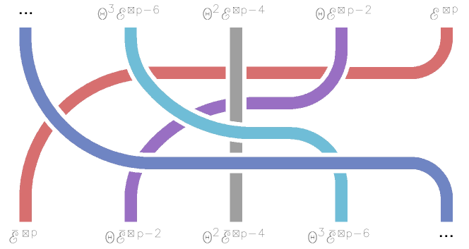
Figure 14.

Theorem 6.14.

Each of the four mega-blocks of Theorem 1.1 can be alternatively (and independently of the other mega-blocks) decomposed as follows:

$$\Bigl{\langle}\bigl{\langle}{\theta}^{1-g+k}\otimes\bar{\operatorname{\mathcal{E}}}^{\boxtimes g-2-2k}\bigr{\rangle}_{0\leq k\leq\lfloor{g-2\over 2}\rfloor},\quad\bigl{\langle}{\theta}^{2-g+k}\otimes\bar{\operatorname{\mathcal{E}}}^{\boxtimes g-3-2k}\bigr{\rangle}_{0\leq k\leq\lfloor{g-3\over 2}\rfloor},\quad{}$$

$${}\quad\bigl{\langle}{\theta}^{2-g+k}\otimes\bar{\operatorname{\mathcal{E}}}^{\boxtimes g-2-2k}\bigr{\rangle}_{0\leq k\leq\lfloor{g-2\over 2}\rfloor},\quad\bigl{\langle}{\theta}^{2-g+k}\otimes\bar{\operatorname{\mathcal{E}}}^{\boxtimes g-1-2k}\bigr{\rangle}_{0\leq k\leq\lfloor{g-1\over 2}\rfloor}\Bigr{\rangle}.$$

Within the mega-blocks with $\bar{\operatorname{\mathcal{E}}}$, the blocks are arranged in increasing order of $k$ (instead of decreasing order of $k$ for the mega-blocks with $\operatorname{\mathcal{E}}$ as in Theorem 1.1). Up to a twist by a tensor power of $\theta$, the decomposition of each mega-block from Theorems 1.1 and 6.14 are related by the mutation of Figure 14. Here the first block in the top row (and the last block in the bottom row) is given by $\theta^{l}$ if $p=2l$ and by $\theta^{l}\otimes\operatorname{\mathcal{E}}=\theta^{l}\otimes\bar{\operatorname{\mathcal{E}}}$ if $p=2l+1$.

Proof.

We start with a semi-orthogonal decomposition of Theorem 1.1 with mega-blocks that we denote by $\operatorname{\mathcal{A}},\operatorname{\mathcal{B}},\operatorname{\mathcal{C}},\operatorname{\mathcal{D}}$. For each Fourier–Mukai functor $\operatorname{\mathcal{P}}_{\operatorname{\mathcal{G}}}:\,D^{b}(\operatorname{Sym}^{k}C)\to D^{b}(N)$ used in it, we consider a fully faithful functor $D^{b}(\operatorname{Sym}^{k}C)\to D^{b}(N)$ given by $T\mapsto(\operatorname{\mathcal{P}}_{\operatorname{\mathcal{G}}}(T^{*}))^{*}$. By coherent duality, the image of this functor agrees with the image of the Fourier–Mukai functor $\operatorname{\mathcal{P}}_{\operatorname{\mathcal{G}}^{*}}:\,D^{b}(\operatorname{Sym}^{k}C)\to D^{b}(N)$ [huybrechts]*Remark 5.8. This gives a semi-orthogonal decomposition with mega-blocks $\operatorname{\mathcal{D}}^{\prime},\operatorname{\mathcal{C}}^{\prime},\operatorname{\mathcal{B}}^{\prime},\operatorname{\mathcal{A}}^{\prime}$ with blocks within mega-blocks arranged in the opposite order to ordering in $\operatorname{\mathcal{A}},\operatorname{\mathcal{B}},\operatorname{\mathcal{C}},\operatorname{\mathcal{D}}$.

We move the mega-block $\operatorname{\mathcal{D}}^{\prime}$ to the right of this decomposition by tensoring it with $\omega_{N}^{*}=\theta^{2}$. Further tensoring with $\theta^{1-g}$ and using that (up to line bundles pulled back from $\operatorname{Sym}^{\alpha}C$) we have $(\operatorname{\mathcal{E}}^{\boxtimes\alpha})^{*}\simeq Z^{-\alpha}(\operatorname{\mathcal{F}}^{\boxtimes\alpha})^{*}\simeq Z^{-\alpha}\operatorname{{\boldsymbol{\Lambda}}}^{-\alpha}\bar{\operatorname{\mathcal{F}}}^{\boxtimes\alpha}\simeq\theta^{-\alpha}\bar{\operatorname{\mathcal{E}}}^{\boxtimes\alpha}$ (see Lemma 3.4), we obtain the semi-orthogonal decomposition of Theorem 6.14 with mega-blocks $\bar{\operatorname{\mathcal{A}}},\bar{\operatorname{\mathcal{B}}},\bar{\operatorname{\mathcal{C}}},\bar{\operatorname{\mathcal{D}}}$.

We claim that $\operatorname{\mathcal{A}}=\bar{\operatorname{\mathcal{A}}}$, $\operatorname{\mathcal{B}}=\bar{\operatorname{\mathcal{B}}}$, $\operatorname{\mathcal{C}}=\bar{\operatorname{\mathcal{C}}}$, and $\operatorname{\mathcal{D}}=\bar{\operatorname{\mathcal{D}}}$. Since both decompositions are full, it suffices to show that each block $X$ from the megablocks $\bar{\operatorname{\mathcal{A}}},\bar{\operatorname{\mathcal{B}}},\bar{\operatorname{\mathcal{C}}},\bar{\operatorname{\mathcal{D}}}$ (resp., $\operatorname{\mathcal{A}},\operatorname{\mathcal{B}},\operatorname{\mathcal{C}},\operatorname{\mathcal{D}}$) is semi-orthogonal (in the correct direction) to each block $Y$ from the megablocks $\operatorname{\mathcal{A}},\operatorname{\mathcal{B}},\operatorname{\mathcal{C}},\operatorname{\mathcal{D}}$ (resp., $\bar{\operatorname{\mathcal{A}}},\bar{\operatorname{\mathcal{B}}},\bar{\operatorname{\mathcal{C}}},\bar{\operatorname{\mathcal{D}}}$) except for the mega-block containing $X$.

Regarding $D^{b}(N)$ as an admissible subcategory of $D^{b}(M)$, we rewrite the kernels in terms of $Z$, $\operatorname{{\boldsymbol{\Lambda}}}$, and $\operatorname{\mathcal{F}}$ using $\operatorname{\mathcal{E}}=Z\operatorname{\mathcal{F}}$ and $\theta=Z^{2}\operatorname{{\boldsymbol{\Lambda}}}$:

$$\operatorname{\mathcal{A}}=\bigl{\langle}Z^{-g}{\operatorname{{\boldsymbol{\Lambda}}}}^{1-g+k}\operatorname{\mathcal{F}}^{\boxtimes g-2-2k}\bigr{\rangle}_{0\leq k\leq\lfloor{g-2\over 2}\rfloor}$$

$$\operatorname{\mathcal{B}}=\bigl{\langle}Z^{-g+1}{\operatorname{{\boldsymbol{\Lambda}}}}^{2-g+k}\operatorname{\mathcal{F}}^{\boxtimes g-3-2k}\bigr{\rangle}_{0\leq k\leq\lfloor{g-3\over 2}\rfloor}$$

$$\operatorname{\mathcal{C}}=\bigl{\langle}Z^{-g+2}{\operatorname{{\boldsymbol{\Lambda}}}}^{2-g+k}\operatorname{\mathcal{F}}^{\boxtimes g-2-2k}\bigr{\rangle}_{0\leq k\leq\lfloor{g-2\over 2}\rfloor}$$

$$\operatorname{\mathcal{D}}=\bigl{\langle}Z^{-g-3}{\operatorname{{\boldsymbol{\Lambda}}}}^{2-g+k}\operatorname{\mathcal{F}}^{\boxtimes g-1-2k}\bigr{\rangle}_{0\leq k\leq\lfloor{g-1\over 2}\rfloor}.$$

$\bar{\operatorname{\mathcal{A}}},\bar{\operatorname{\mathcal{B}}},\bar{\operatorname{\mathcal{C}}},\bar{\operatorname{\mathcal{D}}}$ are the same with $\operatorname{\mathcal{F}}$ replaced by $\bar{\operatorname{\mathcal{F}}}$. As usual, it suffices to check semi-orthogonality at closed points; in what follows, we let $D,D^{\prime}$ be effective divisors on $C$ of appropriate degree. First we show $\operatorname{\mathcal{A}}\subset\bar{\operatorname{\mathcal{B}}}^{\perp}\cap\bar{\operatorname{\mathcal{C}}}^{\perp}\cap\bar{\operatorname{\mathcal{D}}}^{\perp}$. We have

$$R\Gamma(Z^{-1}\operatorname{{\boldsymbol{\Lambda}}}^{l-k-1}(\bar{\operatorname{\mathcal{F}}}^{\boxtimes g-3-2k}_{D})^{*}\otimes\operatorname{\mathcal{F}}^{\boxtimes g-2-2l}_{D^{\prime}})=0$$

by [TT]*Theorem 4.1, so $\operatorname{\mathcal{A}}\subset\bar{\operatorname{\mathcal{B}}}^{\perp}$ (note that $-3-2k<l-k-1<2l+1$). Recalling that $\omega_{M}=Z^{-1}\theta^{-1}\operatorname{{\boldsymbol{\Lambda}}}^{-1}=Z^{-3}\operatorname{{\boldsymbol{\Lambda}}}^{-2}$, we have

$$R\Gamma (Z^{-2}\operatorname{{\boldsymbol{\Lambda}}}^{l-k-1}(\bar{\operatorname{\mathcal{F}}}^{\boxtimes g-2-2k}_{D})^{*}\otimes\operatorname{\mathcal{F}}^{\boxtimes g-2-2l}_{D^{\prime}})$$

$$=R\Gamma (Z^{-1}\operatorname{{\boldsymbol{\Lambda}}}^{k-l-1}({\operatorname{\mathcal{F}}}^{\boxtimes g-2-2l}_{D^{\prime}})^{*}\otimes\bar{\operatorname{\mathcal{F}}}^{\boxtimes g-2-2k}_{D})[3g-3]=0$$

by Serre duality and [TT]*Theorem 4.1 (we have $-2-2l<k-l-1<2k+1$). Hence $A\subset\bar{\operatorname{\mathcal{C}}}^{\perp}$. Finally, Serre duality and $(\operatorname{\mathcal{F}}^{\boxtimes\alpha}_{D})^{*}=\operatorname{{\boldsymbol{\Lambda}}}^{-\alpha}\bar{\operatorname{\mathcal{F}}}^{\boxtimes\alpha}_{D}$ gives

$$R\Gamma (Z^{-3}\operatorname{{\boldsymbol{\Lambda}}}^{l-k-1}(\bar{\operatorname{\mathcal{F}}}^{\boxtimes g-1-2k}_{D})^{*}\otimes\operatorname{\mathcal{F}}^{\boxtimes g-2-2l}_{D^{\prime}})$$

$$=R\Gamma (\operatorname{{\boldsymbol{\Lambda}}}^{k-l-1}({\operatorname{\mathcal{F}}}^{\boxtimes g-2-2l}_{D^{\prime}})^{*}\otimes\bar{\operatorname{\mathcal{F}}}^{\boxtimes g-1-2k}_{D})[3g-3]$$

$$=R\Gamma (\operatorname{{\boldsymbol{\Lambda}}}^{l-k}({\operatorname{\mathcal{F}}}^{\boxtimes g-1-2k}_{D})^{*}\otimes\bar{\operatorname{\mathcal{F}}}^{\boxtimes g-2-2l}_{D^{\prime}})[3g-3].$$

Since $-2-2l<k-l-1<2k+1$, $-1-2k<l-k<2l+2$, and either $k-l-1<0$ or $l-k<0$, this vanishes by Theorem 3.8, giving $A\subset\bar{\operatorname{\mathcal{D}}}^{\perp}$.

Next, we show that $\bar{\operatorname{\mathcal{A}}}\subset\operatorname{\mathcal{B}}^{\perp}\cap\operatorname{\mathcal{C}}^{\perp}\cap\operatorname{\mathcal{D}}^{\perp}$. That $\bar{\operatorname{\mathcal{A}}}\subset\operatorname{\mathcal{B}}^{\perp}$ and $\bar{\operatorname{\mathcal{A}}}\subset\operatorname{\mathcal{C}}^{\perp}$ follows from [TT]*Theorem 4.1 just as above with $\operatorname{\mathcal{F}}$ and $\bar{\operatorname{\mathcal{F}}}$ exchanged. For $\bar{\operatorname{\mathcal{A}}}\subset\operatorname{\mathcal{D}}^{\perp}$, we need to show that

$$R\Gamma(\operatorname{{\boldsymbol{\Lambda}}}^{k-l-1}(\bar{\operatorname{\mathcal{F}}}^{\boxtimes g-2-2l}_{D^{\prime}})^{*}\otimes\operatorname{\mathcal{F}}^{\boxtimes g-1-2k}_{D})[3g-3]=0,$$

which follows from Lemma 5.4 and Remark 5.7: we have $-2-2l<k-l-1<2k+1$ and $2(k-l-1)<2k-2l-1.$

It remains to show that $\operatorname{\mathcal{B}}\subset\bar{\operatorname{\mathcal{C}}}^{\perp}\cap\bar{\operatorname{\mathcal{D}}}^{\perp}$, $\operatorname{\mathcal{C}}\subset\bar{\operatorname{\mathcal{D}}}^{\perp}$, $\bar{\operatorname{\mathcal{B}}}\subset\operatorname{\mathcal{C}}^{\perp}\cap\operatorname{\mathcal{D}}^{\perp}$, and $\bar{\operatorname{\mathcal{C}}}\subset\operatorname{\mathcal{D}}^{\perp}$. These follow from [TT]*Theorem 4.1: We have

$$R\Gamma(Z^{-1}\operatorname{{\boldsymbol{\Lambda}}}^{l-k}(\bar{\operatorname{\mathcal{F}}}^{\boxtimes g-2-2k}_{D})^{*}\otimes\operatorname{\mathcal{F}}^{\boxtimes g-3-2l}_{D^{\prime}})=0,$$

since $-2-2k<l-k<2l+2$, so $\operatorname{\mathcal{B}}\subset\bar{\operatorname{\mathcal{C}}}^{\perp}$. Then

$$R\Gamma (Z^{-2}\Lambda^{l-k}(\bar{\operatorname{\mathcal{F}}}^{\boxtimes g-1-2k}_{D})^{*}\otimes\operatorname{\mathcal{F}}^{\boxtimes g-3-2l}_{D^{\prime}})$$

$$=R\Gamma (Z^{-1}\Lambda^{k-l-2}(\operatorname{\mathcal{F}}^{\boxtimes g-3-2l}_{D^{\prime}})^{*}\otimes\bar{\operatorname{\mathcal{F}}}^{\boxtimes g-1-2k}_{D})=0,$$

since $-3-2l<k-l-2<2k$, so $\operatorname{\mathcal{B}}\subset\bar{\operatorname{\mathcal{D}}}^{\perp}$. Finally,

$$R\Gamma(Z^{-1}\Lambda^{l-k}(\bar{\operatorname{\mathcal{F}}}^{\boxtimes g-1-2k}_{D})^{*}\otimes\operatorname{\mathcal{F}}^{\boxtimes g-2-2l}_{D^{\prime}})=0,$$

since $-1-2k<l-k<2l+1$, so $\operatorname{\mathcal{C}}\subset\bar{\operatorname{\mathcal{D}}}^{\perp}$. Exchanging $\operatorname{\mathcal{F}}$ and $\bar{\operatorname{\mathcal{F}}}$ above yields $\bar{\operatorname{\mathcal{B}}}\subset\operatorname{\mathcal{C}}^{\perp}\cap\operatorname{\mathcal{D}}^{\perp}$, and $\bar{\operatorname{\mathcal{C}}}\subset\operatorname{\mathcal{D}}^{\perp}$, as desired.

Now that we know that megablocks in Theorems 1.1 and 6.14 are the same, we proceed with proving that blocks within them are related by the mutation from Figure 14. We argue by induction on $p$. By the inductive assumption, we can mutate all blocks except $\operatorname{\mathcal{E}}^{\boxtimes p}$ in the top row of Figure 14 into the corresponding blocks of the bottom row, as indicated. It remains to show that the block $\operatorname{\mathcal{E}}^{\boxtimes p}$ mutates into the block $\bar{\operatorname{\mathcal{E}}}^{\boxtimes p}$. Since the bottom row of the mutation of Figure 14 is a semi-orthogonal decomposition, this is clear. ∎

References

[1]
Semiorthogonal decomposition for algebraic varietiesBondalA.OrlovD.1995https://arxiv.org/abs/alg-geom/9506012@article{bondal-orlov,
title = {Semiorthogonal decomposition for algebraic varieties},
author = {Bondal, A.},
author = {Orlov, D.},
date = {1995},
eprint = {https://arxiv.org/abs/alg-geom/9506012}}
[3]
CastravetAna-MariaTevelevJeniaDerived category of moduli of pointed curves – iAlgebr. Geom.720206722–757ISSN 2313-1691@article{castravet1,
author = {Castravet, Ana-Maria},
author = {Tevelev, Jenia},
title = {Derived category of moduli of pointed curves~–~I},
journal = {Algebr. Geom.},
volume = {7},
date = {2020},
number = {6},
pages = {722–757},
issn = {2313-1691}}
[5]
CastravetAna-MariaTevelevJeniaDerived category of moduli of pointed curves – iihttps://arxiv.org/abs/2002.028892020@article{castravet2,
author = {Castravet, Ana-Maria},
author = {Tevelev, Jenia},
title = {Derived category of moduli of pointed curves~–~II},
eprint = {https://arxiv.org/abs/2002.02889},
date = {2020}}
[7]
DrezetJ.-M.NarasimhanM.S.Invent. math.153–94Groupe de picard des variétés de modules de fibrés semi-stables sur les courbes algébriques971989@article{DN,
author = { Drezet, J.-M.},
author = {Narasimhan, M.S.},
journal = {Invent. math.},
number = {1},
pages = {53–94},
title = {Groupe de Picard des vari\'et\'es de modules de fibr\'es semi-stables sur les courbes alg\'ebriques},
volume = {97},
year = {1989}}
[9]
HuybrechtsD.Fourier-mukai transforms in algebraic geometryOxford Mathematical MonographsThe Clarendon Press, Oxford University Press, Oxford2006viii+307ISBN 978-0-19-929686-6ISBN 0-19-929686-3@book{huybrechts,
author = {Huybrechts, D.},
title = {Fourier-Mukai transforms in algebraic geometry},
series = {Oxford Mathematical Monographs},
publisher = {The Clarendon Press, Oxford University Press, Oxford},
date = {2006},
pages = {viii+307},
isbn = {978-0-19-929686-6},
isbn = {0-19-929686-3}}
[11]
Derived categories of thaddeus pair moduli spaces via d-critical flipsAdvances in Mathematics3911079652021ISSN 0001-8708KosekiNaokiTodaYukinobu@article{kosekitoda,
title = {Derived categories of Thaddeus pair moduli spaces via d-critical flips},
journal = {Advances in Mathematics},
volume = {391},
pages = {107965},
year = {2021},
issn = {0001-8708},
author = {Koseki, Naoki},
author = {Toda, Yukinobu}}
[13]
OrlovD. O.Projective bundles, monoidal transformations, and derived categories of coherent sheavesIzv. Ross. Akad. Nauk Ser. Mat.5619924852–862ISSN 1607-0046@article{orlov,
author = {Orlov, D. O.},
title = {Projective bundles, monoidal transformations, and derived
categories of coherent sheaves},
journal = {Izv. Ross. Akad. Nauk Ser. Mat.},
volume = {56},
date = {1992},
number = {4},
pages = {852–862},
issn = {1607-0046}}
[15]
TevelevJeniaTorresSebástianBGMN conjecture via stable pairshttps://arxiv.org/abs/2108.119512021@article{TT,
author = {Tevelev, Jenia},
author = {Torres, Seb\'astian},
title = {BGMN conjecture via stable pairs},
eprint = {https://arxiv.org/abs/2108.11951},
date = {2021}}
[17]
ThaddeusMichaelStable pairs, linear systems and the verlinde formulaInvent. Math.11719942317–353ISSN 0020-9910@article{thaddeus,
author = {Thaddeus, Michael},
title = {Stable pairs, linear systems and the Verlinde formula},
journal = {Invent. Math.},
volume = {117},
date = {1994},
number = {2},
pages = {317–353},
issn = {0020-9910}}
[19]
TodaYukinobuSemiorthogonal decompositions of stable pair moduli spaces via d-critical flipsJ. Eur. Math. Soc.2320211675–1725@article{toda,
author = {Toda, Yukinobu},
title = {Semiorthogonal decompositions of stable pair moduli spaces via d-critical flips},
journal = {J. Eur. Math. Soc.},
volume = {23},
year = {2021},
pages = {1675–1725}}
[21]
TorresSebastiánBott vanishing using git and quantizationMichigan Math. J., to appearhttps://arxiv.org/abs/2003.106172020@article{myself,
author = {Torres, Sebasti\'an},
title = {Bott vanishing using GIT and quantization},
journal = {Michigan Math. J., to appear},
eprint = {https://arxiv.org/abs/2003.10617},
date = {2020}}