$\gamma Z$-Exchange Contributions in Low-Energy Parity-Violating $ep$ Scattering

Abstract

In this work, the $\gamma Z$-exchange contributions in the low-energy elastic parity-violating $ep$ scattering are discussed with the approximation $m_{e}=0$. By expanding the $\gamma pp$ and $Zpp$ interactions on the momentum of photon and considering both the leading-order and the next-to-leading order interactions, we calculate the amplitudes of the $\gamma Z$-exchange diagrams. After performing the loop integral, we expand the results in the low energy limit, and obtain the analytic expressions for the amplitudes. Numerical comparisons show that the analytic expressions are very close to the full results over a large region. We investigate the power behaviors of the these contributions and find that some are enhanced by a kinematic factor in the low energy limit. Additional, in some cases, the imaginary parts of the contributions from the next-to-leading-order interactions are at the same order as those from the leading-order interactions. Furthermore, the corresponding contributions to the physical observable quantity $A_{PV}$ are also discussed. Combining all the properties together, we conclude that, these analytic expressions describe the leading-order contributions of all $\gamma Z$-exchange helicity amplitudes in the region with $\alpha_{e}\ll Q/M_{N}\sim\delta/M_{N}^{2}\ll 1$, where $\alpha_{e}$ is the fine structure constant, $M_{N}$ is the mass of proton, $Q$ and $\delta$ are the small quantities related to the momentum transfer and the center-of-mass energy.

I Introduction

The parity-violating effects in the elastic $ep$ scattering provide the way to extract the weak charge of proton $Q_{W}$ and the weak form factors of the proton $F_{1,2,3}^{(Zpp)}$. Usually, the measurement of the parity-violating asymmetry $A_{PV}\equiv(\sigma^{+}-\sigma^{-})/(\sigma^{+}+\sigma^{-})$ is used to extract these quantities Kaplan1988 ; SAMPLE ; HAPPEX ; A4 ; G0 ; Qweak ; P2 . To extract these physical quantities precisely, the virtual radiative and the real radiative corrections should be estimated carefully. Among all the virtual radiative corrections, the contributions from the $\gamma Z$-exchange are the most special one since their effects can not be absorbed by some constants even when the momentum transfer is fixed. In literatures, a few methods have been used to estimated the $\gamma Z$-exchange contributions to $A_{PV}$, such as the traditional calculation with zero energy approximation ep-ep-gammaZ-zero-energy , the hadronic model ep-ep-gammaZ-hadronic-model-method , the general partonic distributions (GPDs) ep-ep-gammaZ-GPD-method and the dispersion relations (DRs) method ep-ep-gammaZ-dispersion-relation-1 ; ep-ep-gammaZ-dispersion-relation-2 .

In this work, we discuss the $\gamma Z$-exchange contributions from a different perspective. We use the low-energy $\gamma pp$ and $Zpp$ interactions, which are expanded on the momentum to the leading-order (LO) and the next-to-leading-order (NLO), to calculate the $\gamma Z$-exchange amplitudes. The similar method has been used to discuss the two-photon-exchange (TPE) contributions in the elastic $ep$ and $\mu p$ scattering lp-lp-TPE-chiral . In this work, we present the analytic expressions for the $\gamma Z$-exchange contributions at the amplitude level in the low energy limit. These expressions show several interesting properties, which are not readily apparent in the direct numerical results or the conventional estimation of the $\gamma Z$-exchange contributions to $A_{PV}$.

The paper is organized as following, in section II, at first we take the $\gamma pp$ and $Zpp$ interactions in the low energy limit as examples to write down the $\gamma Z$-exchange amplitudes and express the amplitudes as linear sums of some general invariant amplitudes. Then we discuss our approach to calculate the corresponding coefficients of the invariant amplitudes in dimension regularization. The relations between the invariant amplitudes and the helicity amplitudes in the center-of-mass frame are also given. In sections III, we give the analytic expressions for the $\gamma Z$-exchange contributions to the coefficients and the helicity amplitudes in the low energy limit. For comparison, the corresponding contributions to the physical quantity $A_{PV}$ are also given. In section IV, we present the numeric comparison between the analytic results and the full numeric results. In section V, we discuss the properties of these contributions. Also some properties of the results with other interactions as inputs are discussed.

II Basic formulas

II.1 $\gamma Z$-exchange contributions in $ep\rightarrow ep$ at low energy

For the elastic $ep$ scattering, the parity-conserving diagram in the LO of the coupling constant is shown as Fig. 1($a$) where we label the momenta of the incoming electron, the incoming proton, the outgoing electron and the outgoing proton as $p_{1,2,3,4}$, respectively. The parity-violating contribution in the LO of coupling constant is from the one-$Z$-exchange diagram, as shown in Fig. 1($b$).

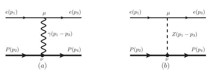
Figure 1: The tree diagrams for $ep\rightarrow ep$: ($a$) is the one-photon-exchange diagram and ($b$) is the one-$Z$-exchange diagram.

When one goes beyond the tree level, the radiative corrections should be considered. Among all the virtual radiative corrections, the contributions from $\gamma Z$-exchange and $WW$-exchange play special roles since their contributions are not only dependent on the momentum transfer but also dependent on the center-of-mass energy. The contributions from $WW$-exchange ep-ep-gammaZ-zero-energy can be well estimated since their contributions are dominated in the region where the two $W$ bosons’ momenta are large, while the contributions from $\gamma Z$-exchange are much different. In this work, we limit our discussion in the low energy limit where the momentum transfer goes to zero and the center-of-mass energy goes to the minimum physical value at fixed momentum transfer. In this limit, a naive picture is that only the interactions with the LO and the NLO of the momenta give the main contributions. This argument has been used to estimate the TPE contributions in $ep,\mu p$ scattering lp-lp-TPE-chiral . In this work, we take the similar assumption to discuss the low energy behaviors of the $\gamma Z$-exchange contributions at first, and then go back check its validity.

Naively, for the $\gamma Z$-exchange contributions in the low energy limit, only the elastic intermediate state gives the contributions, which can be described by the diagrams shown in Fig. (2).

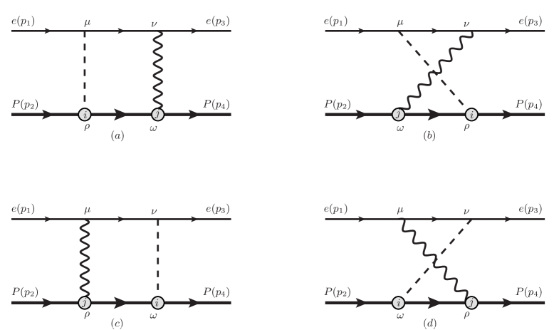
Figure 2: The $\gamma$Z-exchange diagrams of $ep\rightarrow ep$: ($a,c$) are the box diagrams and ($b,d$) are the crossed-box diagrams.

Generally, the interactions between the vector bosons and the proton are dependent on the momentum transfer. In literatures, the form factors are usually introduced to describe the structure of proton. At the low energy scale, the form factors can be expanded on the momentum transfer order by order, the LO and the NLO interactions are expressed as

$$\Gamma^{\mu}_{\gamma ee} = -ie\gamma^{\mu},~{}~{}~{}~{}\Gamma^{\mu}_{Zee}=-i[g_{e}^{V}\gamma^{\mu}+g_{e}^{A}\gamma^{\mu}\gamma_{5}],$$

$$\Gamma^{\mu}_{\gamma pp,0} = ieF_{1}\gamma^{\mu},~{}~{}~{}~{}\Gamma^{\mu}_{\gamma pp,1}=ieF_{2}\frac{i\sigma^{\mu\nu}}{2M_{N}}q_{\nu},$$

$$\Gamma^{\mu}_{Zpp,0} = -i[g_{1}\gamma^{\mu}+g_{3}\gamma^{\mu}\gamma^{5}],~{}~{}~{}~{}\Gamma^{\mu}_{Zpp,1}=-ig_{2}\frac{i\sigma^{\mu\nu}}{2M_{N}}q_{\nu},$$ (1)

where $g_{e}^{V,A}$ are the coupling constants of the $Zee$ interactions, $F_{1,2}$ are the coupling constants of the $\gamma pp$ interactions in the low energy limit, and $g_{1,2,3}$ are the coupling constants of $Zpp$ interactions in the low energy limit, $q$ is the momentum of the incoming boson, the label $0$ refers to the LO interactions which are not dependent on the boson’s momentum, and the label 1 refers to the NLO interactions which are proportion to the boson’s momentum.

By these interactions, the corresponding $\gamma Z$-exchange amplitudes can be expressed as

$${\cal M}^{(a)}_{ij} = -i\bar{\mu}^{2\epsilon}\int\frac{\textrm{d}^{d}l}{(2\pi)^{d}}\bar{u}_{3}\Gamma^{\nu}_{\gamma ee}S_{e}(p_{3}+l)\Gamma^{\mu}_{Zee}u_{1}\bar{u}_{4}\Gamma^{\omega}_{\gamma pp,j}(p_{4},p_{4}-l)S_{p}(p_{4}-l)\Gamma^{\rho}_{Zpp,i}(p_{4}-l,p_{2})u_{2}$$

$$\times D_{\nu\omega}^{\gamma}(l)D_{\mu\rho}^{Z}(p_{1}-p_{3}-l),$$

$${\cal M}^{(b)}_{ij} = -i\bar{\mu}^{2\epsilon}\int\frac{\textrm{d}^{d}l}{(2\pi)^{d}}\bar{u}_{3}\Gamma^{\nu}_{\gamma ee}S_{e}(p_{3}+l)\Gamma^{\mu}_{Zee}u_{1}\bar{u}_{4}\Gamma^{\rho}_{Zpp,i}(p_{4},p_{2}+l)S_{p}(p_{2}+l)\Gamma^{\omega}_{\gamma pp,j}(p_{2}+l,p_{2})u_{2}$$

$$\times D_{\nu\omega}^{\gamma}(l)D_{\mu\rho}^{Z}(p_{1}-p_{3}-l),$$

$${\cal M}^{(c)}_{ij} = -i\bar{\mu}^{2\epsilon}\int\frac{\textrm{d}^{d}l}{(2\pi)^{d}}\bar{u}_{3}\Gamma^{\nu}_{Zee}S_{e}(p_{1}-l)\Gamma^{\mu}_{\gamma ee}u_{1}\bar{u}_{4}\Gamma^{\omega}_{Zpp,i}(p_{4},p_{2}+l)S_{p}(p_{2}+l)\Gamma^{\rho}_{\gamma pp,j}(p_{2}+l,p_{2})u_{2}$$

$$\times D_{\nu\omega}^{\gamma}(l)D_{\mu\rho}^{Z}(p_{1}-p_{3}-l),$$

$${\cal M}^{(d)}_{ij} = -i\bar{\mu}^{2\epsilon}\int\frac{d^{d}l}{(2\pi)^{d}}\bar{u}_{3}\Gamma^{\nu}_{Zee}S_{e}(p_{1}-l)\Gamma^{\mu}_{\gamma ee}u_{1}\bar{u}_{4}\Gamma^{\rho}_{\gamma pp,j}(p_{4},p_{4}-l)S_{p}(p_{4}-l)\Gamma^{\omega}_{Zpp,i}(p_{4}-l,p_{2})u_{2}$$

$$\times D_{\nu\omega}^{\gamma}(l)D_{\mu\rho}^{Z}(p_{1}-p_{3}-l),$$ (2)

where $\bar{u}_{i},u_{i}$ are the short writing of the spinors $\bar{u}(p_{i},s_{i}),u(p_{i},s_{i})$ with corresponding masses, $l$ is the momentum of photon, $i$ and $j$ refer to the order of the momentum in the vertices $\Gamma_{\gamma pp}$ and $\Gamma_{Zpp}$, $\bar{\mu}$ is the renormalization scale and $\epsilon=4-d$ with $d$ the dimension. In the naive picture, the label $ij=00$ is corresponding to the LO contribution, $ij=01,10$ are corresponding to the NLO contributions, and $ij=22$ is corresponding to the next-to-next-leading-order (NNLO) contribution. In the practical calculation, we keep all these contributions for comparison.

In the practical calculation, the package FeynCalc10.0 FenyCalc is used to deal with Dirac matrix, the Package PackageX3.0 PacakgeX is used to do the loop integration and the the package LoopTools LoopTools is used for double check.

II.2 The scheme to deal with $\gamma_{5}$ in $d$-dimension and the general invariant amplitudes

To calculate the amplitudes ${\cal M}^{(a,b,c,d)}_{ij}$ in the dimension regularization, one should choose a scheme to deal with the Dirac matrix $\gamma_{5}$ in $d$-dimension. This is a little different from the similar calculation in the parity-conserving $ep$ scattering since , in principle, this is no $\gamma_{5}$ at the amplitude level in the latter case. In the practical calculation, we choose the NDR scheme in FeynCalc FenyCalc to deal with $\gamma_{5}$.

In the NDR scheme, there is ambiguous definition for the trace of a matrix with odd $\gamma_{5}$. To avoid such ambiguous definition in the calculation, we separate the full amplitude into a parity conserved (PC) part and a parity violated (PV) part, and then separate the PV part as following:

$${\cal M}^{(a+b+c+d)}_{\gamma Z} \equiv {\cal M}^{\textrm{PC}}_{\gamma Z}+{\cal M}^{\textrm{PV}}_{\gamma Z},$$

$${\cal M}^{\textrm{PV}}_{\gamma Z} \equiv g_{e}^{A}{\cal M}^{V}_{\gamma Z}+g_{e}^{V}{\cal M}^{A}_{\gamma Z}.$$ (3)

Since we focus on the PV part of the amplitude, we only discuss the amplitudes ${\cal M}^{V}_{\gamma Z}$ and ${\cal M}^{A}_{\gamma Z}$ in the following. After taking the approximation $m_{e}=0$ with $m_{e}$ the mass of electron, the amplitudes ${\cal M}^{V,A}_{\gamma Z}$ can be written as

$${\cal M}^{V}_{\gamma Z} \equiv \sum_{i=1}^{3}{\cal F}_{\gamma Z,i}^{V}{\cal P}_{i}^{V}\equiv\sum\limits_{i=1}^{3}\sum\limits_{j=1}^{2}\sum\limits_{k=1}^{2}{\cal C}_{\gamma Z,ijk}^{V}F_{j}g_{k}{\cal P}_{i}^{V},$$

$${\cal M}^{A}_{\gamma Z} \equiv \sum_{i=1}^{3}{\cal F}_{\gamma Z,i}^{A}\mathcal{P}_{i}^{A}\equiv\sum\limits_{i=1}^{3}\sum\limits_{j=1}^{2}{\cal C}_{\gamma Z,ij3}^{A}F_{j}g_{3}{\cal P}_{i}^{A},$$ (4)

where the general invariant amplitudes ${\cal P}_{i}^{V}$ and ${\cal P}_{i}^{A}$ are chosen as

$${\cal P}_{1}^{V} \equiv \left[\bar{u}_{3}\gamma_{\mu}\gamma_{5}u_{1}\right]\left[\bar{u}_{4}\gamma^{\mu}u_{2}\right],$$

$${\cal P}_{2}^{V} \equiv \frac{1}{Q}\left[\bar{u}_{3}\gamma_{\mu}\gamma_{5}u_{1}\right]\left[\bar{u}_{4}i\sigma^{\mu\nu}q_{\nu}u_{2}\right],$$

$${\cal P}_{3}^{V} \equiv \frac{1}{M_{N}Q}\left[\bar{u}_{3}P\!\!\!\!/\gamma_{5}u_{1}\right]\left[\bar{u}_{4}K\!\!\!\!/u_{2}\right],$$

$${\cal P}_{1}^{A} \equiv \left[\bar{u}_{3}\gamma^{\mu}u_{1}\right]\left[\bar{u}_{4}\gamma_{\mu}\gamma_{5}u_{2}\right],$$

$${\cal P}_{2}^{A} \equiv \frac{1}{Q}\left[\bar{u}_{3}\gamma^{\mu}u_{1}\right]\left[\bar{u}_{4}\gamma_{\mu}K\!\!\!\!/\gamma_{5}u_{2}\right],$$

$${\cal P}_{3}^{A} \equiv \frac{1}{M_{N}Q}\left[\bar{u}_{3}P\!\!\!\!/u_{1}\right]\left[\bar{u}_{4}K\!\!\!\!/\gamma_{5}u_{2}\right],$$ (5)

with $P=p_{2}+p_{4}$, $K=p_{1}+p_{3}$, $Q^{2}=-q^{2}$, $q=p_{4}-p_{2}=p_{1}-p_{3}$, and $M_{N}$ the mass of proton.

Such separation is a little different from the form used in the references where usually only three invariant amplitudes are chosen ep-ep-gammaZ-dispersion-relation-1 . As we argued above, the reason of such separation is to avoid the ambiguous definition of $\gamma_{5}$ in $d$-dimension. By these definitions, now there is only even $\gamma_{5}$ in the following calculation of the coefficients $C_{\gamma Z,ijk}^{V}$ and $C_{\gamma Z,ij3}^{A}$.

Similarly, we separate the one-$Z$-exchange amplitude ${\cal M}_{Z}$ as

$${\cal M}_{Z} \equiv {\cal M}^{\textrm{PC}}_{Z}+{\cal M}^{\textrm{PV}}_{Z},$$

$${\cal M}^{\textrm{PV}}_{Z} \equiv g_{e}^{A}{\cal M}^{V}_{Z}+g_{e}^{V}{\cal M}^{A}_{Z},$$

$${\cal M}_{Z}^{X} \equiv \sum_{i=1}^{3}{\cal F}_{Z,i}^{X}{\cal P}_{i}^{X},$$ (6)

with $X=V$ or $A$, respectively.

II.3 Calculation of $C_{\gamma Z,ijk}^{V}$ and $C_{\gamma Z,ijk}^{A}$

To calculate the coefficients $C_{\gamma Z,ijk}^{V}$ and $C_{\gamma Z,ijk}^{A}$, one can solve the following algebraic equations in $d-$dimension

$$\sum_{helicity}{\cal M}^{V}_{\gamma Z}{\cal T}_{n}^{V*} = \sum_{helicity}\sum_{i=1}^{3}{\cal F}_{\gamma Z,i}^{V}{\cal P}_{i}^{V}{\cal T}_{n}^{V*}=\sum_{helicity}\sum\limits_{i=1}^{3}\sum\limits_{j=1}^{2}\sum\limits_{k=1}^{2}{\cal C}_{\gamma Z,ijk}^{V}F_{j}g_{k}{\cal M}_{i}^{V}{\cal T}_{n}^{V*},$$

$$\sum_{helicity}{\cal M}^{A}_{\gamma Z}{\cal T}_{n}^{V*} = \sum_{helicity}\sum_{i=1}^{3}{\cal F}_{\gamma Z,i}^{A}{\cal P}_{i}^{A}{\cal T}_{n}^{A*}=\sum_{helicity}\sum\limits_{i=1}^{3}\sum\limits_{j=1}^{2}{\cal C}_{\gamma Z,ij3}^{A}F_{j}g_{3}{\cal M}_{i}^{A}{\cal T}_{n}^{A*},$$ (7)

where ${\cal T}_{n}^{V}$ or ${\cal T}_{n}^{A}$ can be chosen as ${\cal P}_{n}^{V}$ or ${\cal P}_{n}^{A}$ directly.

After calculating the following matrix in $d$-dimension,

$$\mathcal{D}_{ij}^{X} \equiv \sum_{helicity}{\cal P}_{i}^{X}{\cal P}_{j}^{X*},$$ (8)

the coefficients ${\cal F}^{X}_{\gamma Z,i}$ can be written as

$${\cal F}^{X}_{\gamma Z,i} = \sum_{j}[(\mathcal{D}^{X})^{-1}]_{ij}\sum_{helicity}{\cal M}^{X}_{\gamma Z}{\cal P}_{j}^{*}.$$ (9)

When ${\cal F}^{X}_{\gamma Z,i}$ are known, the corresponding coefficients $C_{\gamma Z,ijk}^{X}$ can be obtained directly.

The expressions of $\mathcal{D}_{ij}^{X}$ in $d$-dimension is a little complex, so we do not list them here.

II.4 From general invariant amplitudes to helicity amplitudes

In some cases, the physical meaning of the general invariant amplitudes and their coefficients are not clear since the behaviors of the coefficients $C_{\gamma Z,ijk}^{X}$ may include some kinematic effects. While, the physical meaning of the helicity amplitudes is much clear.

After some simple calculations, one can find the following properties in the center-of-mass frame

$${\cal M}_{Y}^{+-\pm\pm,\textrm{PV}}={\cal M}_{Y}^{-+\pm\pm,\textrm{PV}}=0,$$

$${\cal M}_{Y}^{++++,\textrm{PV},}=-{\cal M}_{Y}^{----,\textrm{PV}},$$

$${\cal M}_{Y}^{+++-,\textrm{PV}}=-{\cal M}_{Y}^{++-+,\textrm{PV}}=-{\cal M}_{Y}^{--+-,\textrm{PV}}={\cal M}_{Y}^{---+,\textrm{PV}},$$

$${\cal M}_{Y}^{++--,\textrm{PV}}=-{\cal M}_{Y}^{--++,\textrm{PV}},$$ (10)

where the index $Y$ refers to $Z$ or $\gamma Z$, the indexes such as ++++ are corresponding to the helicities of the incoming electron, the outgoing electron, the incoming proton and the outgoing proton, respectively.

The helicity amplitudes can be expressed as

$${\cal M}_{Y}^{\pm\pm\pm\pm,X} = \sum_{i}{\cal F}^{X}_{Y,i}{\cal P}_{i}^{\pm\pm\pm\pm,X}.$$ (11)

In Tab. 1, we present the expressions for ${\cal P}_{i}^{\pm\pm\pm\pm,X}$ in the center-of-mass frame where the momenta are chosen as

$$p_{1}^{\mu} = (E_{c},0,0,E_{c}),$$

$$p_{2}^{\mu} = (\sqrt{M_{N}^{2}+E_{c}^{2}},0,0,-E_{c}),$$

$$p_{3}^{\mu} = (E_{c},E_{c}\sin\theta_{c},0,E_{c}\cos\theta_{c}),$$ (12)

and some variables are defined as

$$s \equiv (p_{1}+p_{2})^{2},$$

$$\nu \equiv 2s-2M_{N}^{2}-Q^{2},$$

$$a \equiv \nu+Q^{2}+2M_{N}Q,$$

$$b \equiv \nu+Q^{2}-2M_{N}Q,$$

$$c \equiv \sqrt{\nu^{2}-4M_{N}^{2}Q^{2}-Q^{4}}.$$ (13)

$i$	$1$	$2$	$3$
${\cal P}^{++++,V}_{i}$	$-\frac{ab}{\nu+Q^{2}}$	$-4M_{N}Q$	$-\frac{c^{2}}{M_{N}Q}$
${\cal P}^{+++-,V}_{i}$	$\frac{2cM_{N}Q}{\nu+Q^{2}}$	$-c$	$2c$
${\cal P}^{++--,V}_{i}$	$-\frac{c^{2}}{\nu+Q^{2}}$	$0$	$-\frac{c^{2}}{M_{N}Q}$
${\cal P}^{++++,A}_{i}$	$-\frac{ab+8M_{N}^{2}Q^{2}}{\nu+Q^{2}}$	$0$	$-\frac{c^{2}}{M_{N}Q}$
${\cal M}^{+++-,A}_{i}$	$-\frac{2cM_{N}Q}{\nu+Q^{2}}$	$-c$	0
${\cal M}^{++--,A}_{i}$	$\frac{c^{2}}{\nu+Q^{2}}$	$0$	$\frac{c^{2}}{M_{N}Q}$

Table 1: The expressions for the invariant amplitudes with special helicities ${\cal P}_{i}^{\pm\pm\pm\pm,X}$ in the center-of-mass frame.

From these expressions, the helicity amplitudes ${\cal M}_{\gamma Z}^{\pm\pm\pm\pm,X}$ can be written as the linear sums of the coefficients $C_{\gamma Z,ijk}^{X}$ directly. For example, one has

$${\cal M}^{++++,V}_{\gamma Z} = -\frac{ab}{\nu+Q^{2}}{\cal F}_{\gamma Z,1}^{V}-4M_{N}Q{\cal F}_{\gamma Z,2}^{V}-\frac{c^{2}}{M_{N}Q}{\cal F}_{\gamma Z,3}^{V},$$ (14)

$$= -\sum\limits_{j=1}^{2}\sum\limits_{k=1}^{2}\Big{[}\frac{ab}{\nu+Q^{2}}C_{\gamma Z,1jk}^{V}+4M_{N}QC_{\gamma Z,2jk}^{V}+\frac{c^{2}}{M_{N}Q}C_{\gamma Z,3jk}^{V}\Big{]}F_{j}g_{k}.$$

III Expressions in the Low energy limit

III.1 $C_{\gamma Z,ijk}^{X}$ when $Q^{2}\rightarrow 0$ and $\nu\rightarrow\nu_{min}$

Before discussing the properties of the coefficients $C_{\gamma Z,ijk}^{X}$ in the low energy limit, for comparison, we list the expressions of ${\cal F}_{Z,i}^{X}$ as following

$$\textrm{Re}[{\cal F}_{Z,1}^{V}] = -\frac{g_{1}}{M_{Z}^{2}},~{}~{}~{}~{}\textrm{Re}[{\cal F}_{Z,2}^{V}]=-\frac{g_{2}}{M_{Z}^{2}}\frac{Q}{2M_{N}},~{}~{}~{}~{}\textrm{Re}[{\cal F}_{Z,3}^{V}]=0,$$

$$\textrm{Re}[{\cal F}_{Z,1}^{A}] = -\frac{g_{3}}{M_{Z}^{2}},~{}~{}~{}~{}\textrm{Re}[{\cal F}_{Z,2}^{A}]=0,~{}~{}~{}~{}~{}~{}~{}~{}~{}~{}~{}~{}~{}~{}~{}~{}~{}~{}\textrm{Re}[{\cal F}_{Z,3}^{A}]=0.$$ (15)

Physically, when $Q^{2}$ is fixed, the physical $\nu$ has a minimum value as

$$\nu_{phs}\geq\nu_{min}=Q\sqrt{4M_{N}^{2}+2Q^{2}+2Q\sqrt{4M_{N}^{2}+Q^{2}}}-Q^{2}.$$ (16)

To calculate $C_{\gamma Z,ijk}^{X}$ in the low energy limit, we expand them at $Q\rightarrow 0$ and $\delta\equiv\nu-\nu_{min}\rightarrow 0$ independently after the loop integration. This is a little different from the usual discussion where $Q\rightarrow 0$ and $E_{e}\rightarrow 0$ are used, with $E_{e}$ the energy of initial electron in the Lab frame. The reason that we do not expand the results on $Q$ and $E_{e}$ is, when $Q$ is fixed, actually $E_{e}$ also has a minimum value, which means that $Q\rightarrow 0$ and $E_{e}\rightarrow 0$ are not completely independent for the physical process.

In the practical calculation, the expansion of $C_{\gamma Z,ijk}^{X}$ on $Q$ and $\delta$ should be done independently, which means the expansion is valid for any $\delta/Q$. The final expressions for the non-zero LO contributions $C_{\gamma Z,ijk}^{X,\textrm{LO}}$ are presented in Appendix A.

We would like to mention that, the contributions which are only dependent on $Q$ but not dependent on $\delta$, have the similar behaviors with the radiative corrections to the vertexes $\Gamma^{\mu}_{\gamma pp}$ and $\Gamma^{\mu}_{Zpp}$. This means that, these contributions can be absorbed into some constants at fixed $Q$. The most important property of the $\gamma Z$-exchange contributions is their $\delta$ dependence at fixed $Q$.

III.2 Helicity amplitudes when $Q^{2}\rightarrow 0$ and $\nu\rightarrow\nu_{min}$

Since the physical meaning of the helicity amplitudes is much definite than the coefficients’, we give the expressions for the helicity amplitudes in the low energy limit in this subsection.

At the tree level, the helicity amplitudes due to the one-$Z$-exchange can be separated as

$${\cal M}_{Z}^{\pm\pm\pm\pm,V} \equiv \sum_{k=1}^{2}{\cal M}_{Z,k}^{\pm\pm\pm\pm,V}g_{k}g_{e}^{A},$$

$${\cal M}_{Z}^{\pm\pm\pm\pm,A} \equiv {\cal M}_{Z,3}^{\pm\pm\pm\pm,A}g_{3}g_{e}^{V}.$$ (17)

After expanding ${\cal M}^{\pm\pm\pm\pm,X}_{Z,k}$ on $Q$ and $\delta$ independently, the non-zero LO contributions ${\cal M}^{\pm\pm\pm\pm,X,\textrm{LO}}_{Z,k}$ are expressed as Tab. 2 with

$$h = \frac{1}{M_{Z}^{2}(2M_{N}Q+\delta)},$$

$$z = \sqrt{(4M_{N}Q+\delta)\delta}.$$ (18)

Hs	$++++$	$+++-$	$++--$
${\cal M}^{\textrm{Hs},V,\textrm{LO}}_{Z,1}$	$hz^{2}$	$-2hzM_{N}Q$	$hz^{2}$
${\cal M}^{\textrm{Hs},V,\textrm{LO}}_{Z,2}$	$2h(2M_{N}Q+\delta)Q^{2}$	$-hz\frac{(2M_{N}Q+\delta)Q}{2M_{N}}$	$0$
${\cal M}^{\textrm{Hs},A,\textrm{LO}}_{Z,3}$	$h(8M_{N}^{2}Q^{2}+z^{2})$	$2hzM_{N}Q$	$-hz^{2}$

Table 2: The expressions for ${\cal M}^{\pm\pm\pm\pm,X,\textrm{LO}}_{Z,k}$ in the center-of-mass frame.

Similarly, the helicity amplitudes due to the $\gamma Z$-exchange can be separated as

$${\cal M}_{\gamma Z}^{\pm\pm\pm\pm,V} \equiv \sum_{jk}{\cal M}_{\gamma Z,jk}^{\pm\pm\pm\pm,V}F_{j}g_{k}g_{e}^{A},$$

$${\cal M}_{\gamma Z}^{\pm\pm\pm\pm,A} \equiv \sum_{j}{\cal M}_{\gamma Z,j3}^{\pm\pm\pm\pm,A}F_{j}g_{3}g_{e}^{V}.$$ (19)

We would like to mention, to obtain the correct expressions for the non-zero LO contributions ${\cal M}_{\gamma Z,jk}^{\pm\pm\pm\pm,X,\textrm{LO}}$, one should not directly substitute $C_{\gamma Z,ijk}^{X,\textrm{LO}}$ into Eq. (11). The reason is that, there are cancellations between the contributions from different $C_{\gamma Z,ijk}^{X,\textrm{LO}}$ in the LO in some specific cases. So to obtain the correct expressions for the non-zero LO contributions ${\cal M}_{\gamma Z,jk}^{\pm\pm\pm\pm,X,\textrm{LO}}$, one should substitute $C_{\gamma Z,ijk}^{X}$ into Eq. (11), then expand ${\cal M}_{\gamma Z,jk}^{\pm\pm\pm\pm,X}$ at $Q\rightarrow 0$ and $\delta\rightarrow 0$. The existence of the cancellations also hints that the helicity amplitudes reflect the physical properties in a more definite way.

The final expressions for the non-zero LO contributions ${\cal M}_{\gamma Z,jk}^{\pm\pm\pm\pm,X,\textrm{LO}}$ are presented in Appendix B.

III.3 $A_{PV}$ when $Q^{2}\rightarrow 0$ and $\nu\rightarrow\nu_{min}$

After the coefficients $C_{\gamma Z,ijk}^{X}$ or ${\cal M}_{\gamma Z,jk}^{\pm\pm\pm\pm,X}$ are gotten, in principle, the $\gamma Z$-exchange contributions to all the related physical quantities can be gotten. In this subsection, we discuss the $\gamma Z$-exchange contributions to the physical measurement $A_{PV}$ which is defined as

$$A_{PV} \equiv \frac{\sum\limits_{helicity}({\cal M}^{+}{\cal M}^{+*}-{\cal M}^{-}{\cal M}^{-*})}{\sum\limits_{helicity}({\cal M}^{+}{\cal M}^{+*}+{\cal M}^{-}{\cal M}^{-*})},$$ (20)

where ${\cal M}^{+,-}$ are the helicity amplitudes in the Lab frame with the incoming electron’s helicity $\pm$, respectively.

At the tree level, where only the contributions from the one-photon exchange and the one-$Z$ exchange diagrams are considered, the corresponding $A_{PV}^{\gamma\otimes Z}$ can be expressed as

$$A_{PV}^{\gamma\otimes Z} = \frac{1}{\sigma}\Big{[}\sum_{i=1}^{2}\sum_{k=1}^{2}{\cal A}_{Z,ik}^{V}F_{i}g_{k}g_{e}^{A}+\sum_{i=1}^{2}{\cal A}_{Z,i3}^{A}F_{i}g_{3}g_{e}^{V}\Big{]},$$ (21)

where

$$\sigma = e^{2}\Big{[}4F_{1}^{2}M_{N}^{2}(4M_{N}^{2}Q^{2}-Q^{4}-\nu^{2})-16F_{1}F_{2}M_{N}^{2}Q^{4}-F_{2}^{2}Q^{2}(4M_{N}^{2}Q^{2}-Q^{4}+\nu^{2})\Big{]}$$ (22)

$$\rightarrow -4e^{2}F_{1}^{2}M_{N}^{2}z^{2},$$

and

$${\cal A}_{Z,11}^{V} = \frac{8}{M_{Z}^{2}}M_{N}^{2}Q^{2}(\nu^{2}-4M_{N}^{2}Q^{2}+Q^{4})\rightarrow\frac{4}{M_{Z}^{2}}M_{N}Q^{2}(4M_{N}Q+\delta)(2M_{N}\delta+Q^{3}),$$

$${\cal A}_{Z,12}^{V} = \frac{16}{M_{Z}^{2}}M_{N}^{2}Q^{6},$$

$${\cal A}_{Z,21}^{V} = \frac{16}{M_{Z}^{2}}M_{N}^{2}Q^{6},$$

$${\cal A}_{Z,22}^{V} = \frac{2}{M_{Z}^{2}}Q^{4}(\nu^{2}+4M_{N}^{2}Q^{2}-Q^{4})\rightarrow\frac{2}{M_{Z}^{2}}Q^{4}(8M_{N}^{2}Q^{2}+z^{2}),$$

$${\cal A}_{Z,13}^{A} = \frac{16}{M_{Z}^{2}}M_{N}^{2}Q^{4}\nu\rightarrow\frac{16}{M_{Z}^{2}}M_{N}^{2}Q^{4}(2M_{N}Q+\delta),$$

$${\cal A}_{Z,23}^{A} = \frac{16}{M_{Z}^{2}}M_{N}^{2}Q^{4}\nu\rightarrow\frac{16}{M_{Z}^{2}}M_{N}^{2}Q^{4}(2M_{N}Q+\delta).$$ (23)

When the interference between the one-photon exchange diagram and $\gamma Z$-exchange diagrams is considered, the corresponding $A_{PV}^{\gamma\otimes\gamma Z}$ is expressed as

$$A_{PV}^{\gamma\otimes\gamma Z} = \sum_{i=1}^{3}{\cal N}_{i}^{V}\textrm{Re}[{\cal F}_{\gamma Z,i}^{V}]g_{e}^{A}+\sum_{i=1}^{3}{\cal N}_{i}^{A}\textrm{Re}[{\cal F}_{\gamma Z,i}^{A}]g_{e}^{V}$$ (24)

$$= \sum_{i=1}^{3}\sum_{j=1}^{2}\sum_{k=1}^{2}{\cal N}_{i}^{V}\textrm{Re}[C_{\gamma Z,ijk}^{V}]F_{j}^{\gamma Z}g_{k}g_{e}^{A}+\sum_{i=1}^{3}\sum_{j=1}^{2}{\cal N}_{i}^{A}\textrm{Re}[C_{\gamma Z,ij3}^{A}]F_{j}^{\gamma Z}g_{3}g_{e}^{V},$$

with

$${\cal N}_{1}^{V} = \frac{8M_{N}^{2}Q^{2}}{\sigma}\Big{[}(4M_{N}^{2}Q^{2}-Q^{4}-\nu^{2})F_{1}^{\gamma}-2Q^{4}F_{2}^{\gamma}\Big{]},$$

$${\cal N}_{2}^{V} = -\frac{4M_{N}Q}{\sigma}\Big{[}8M_{N}^{2}Q^{4}F_{1}^{\gamma}+Q^{2}(4M_{N}^{2}Q^{2}-Q^{4}+\nu^{2})F_{2}^{\gamma}\Big{]},$$

$${\cal N}_{3}^{V} = \frac{8M_{N}Q\nu}{\sigma}(4M_{N}^{2}Q^{2}+Q^{4}-\nu^{2})F_{1}^{\gamma},$$

$${\cal N}_{1}^{A} = -\frac{16M_{N}^{2}Q^{4}\nu}{\sigma}(F_{1}^{\gamma}+F_{2}^{\gamma}),$$

$${\cal N}_{2}^{A} = -\frac{4M_{N}Q^{3}}{\sigma}(8M_{N}^{2}Q^{2}F_{1}^{\gamma}+(4M_{N}^{2}Q^{2}-Q^{4}+\nu^{2})F_{2}^{\gamma}),$$

$${\cal N}_{3}^{A} = \frac{8M_{N}Q^{3}}{\sigma}(4M_{N}^{2}Q^{2}+Q^{4}-\nu^{2})(F_{1}^{\gamma}+F_{2}^{\gamma}),$$ (25)

where we have used the indexes $\gamma$ and $\gamma Z$ in $F_{i}$ to represent which diagrams the coupling constants come from, although they are equal numerically. For example, $F_{1}^{\gamma}$ means it comes from the one-photon exchange diagram and $F_{1}^{\gamma Z}$ means it comes from the $\gamma Z$-exchange diagram.

After substituting $C_{\gamma Z,ijk}^{X}$ into the expression, one can write $A_{PV}^{\gamma\otimes\gamma Z}$ as

$$A_{PV}^{\gamma\otimes\gamma Z} \equiv \frac{1}{\sigma}\Big{\{}\sum_{i=1}^{2}\sum_{j=1}^{2}\sum_{k=1}^{2}\textrm{Re}[{\cal A}_{\gamma Z,ijk}^{V}]F_{i}^{\gamma}F_{j}^{\gamma Z}g_{k}g_{e}^{A}+\sum_{i=1}^{2}\sum_{j=1}^{2}\textrm{Re}[{\cal A}_{\gamma Z,ij3}^{A}]F_{i}^{\gamma}F_{j}^{\gamma Z}g_{3}g_{e}^{V}\Big{\}}$$ (26)

$$\equiv \textrm{Re}[\Box_{\gamma Z}^{V}]+\textrm{Re}[\Box_{\gamma Z}^{A}].$$

Similarly to ${\cal M}_{\gamma Z,jk}^{\pm\pm\pm\pm,X}$, to obtain the non-zero LO contributions ${\cal A}_{\gamma Z,ijk}^{X,\textrm{LO}}$, one should subsitute $C_{\gamma Z,ijk}^{X}$ into the expressions, and then expand them on $Q$ and $\delta$ around 0. The final expressions for the non-zero LO contributions ${\cal A}_{\gamma Z,ijk}^{X,\textrm{LO}}$ are presented in Appendix C.

IV Numerical Properties

Before going to discuss the analytic properties, we perform a numerical comparison of the non-zero LO contributions and the full contributions for different values of $Q$ in the range $(0.05,0.1,0.2,0.5)$ GeV and for different values of $\delta$ in the range $[0,1]$ GeV². We find that the two results are very similar across all these regions. In Fig. 3 and Fig. 4, we take $\textrm{Re}[{\cal M}_{\gamma Z,11}^{++++,V,\textrm{LO}}]$ and $\textrm{Re}[{\cal M}_{\gamma Z,13}^{++++,V,\textrm{LO}}]$ as examples to show the numerical comparison. The comparisons clearly show that the analytic non-zero LO expressions provide a reliable approximation of the full result at the low energy scale.

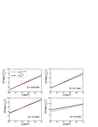
Figure 3: Comparison between $\textrm{Re}[{\cal M}^{++++,V,\textrm{LO}}_{\gamma Z,11}]$ and $\textrm{Re}[{\cal M}^{++++,V}_{\gamma Z,11}]$ at $Q=0.05,0.1,0.2$ and $0.5$ GeV, respectively.

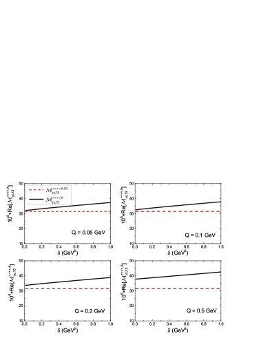
Figure 4: Comparison between $\textrm{Re}[{\cal M}^{++++,A,\textrm{LO}}_{\gamma Z,13}]$ and $\textrm{Re}[{\cal M}^{++++,A}_{\gamma Z,13}]$ at $Q=0.05,0.1,0.2$ and $0.5$ GeV, respectively.

V Power behaviors in the low energy limit

V.1 Power behaviors of $C_{\gamma Z,ijk}^{X}$ in the low energy limit

The analytic expressions for $C_{\gamma Z,ijk}^{X,\textrm{LO}}$ show some very interesting properties. The most important property is about their power behaviors on the variables $Q$ and $\delta$.

To indicate the physical meaning of these power behaviors in a clear way, we take two cases to compare the behaviors. In the first case, we compare the power behaviors of the one-$Z$-exchange contributions and the $\gamma Z$-exchange contributions, where only the LO interactions are considered. In the second case, we compare the power behaviors of the imaginary parts of the $\gamma Z$-exchange contributions from the LO interactions and those from the NLO interactions.

When only the LO interactions are considered, the couplings $F_{2},g_{2}$ are zero and $F_{1}$, $g_{1,3}$ are non-zero. In this case, all the interactions are well defined in the standard model. At the tree level, there are two non-zero PV contributions $\textrm{Re}[{\cal F}_{Z,1}^{V}]$ and $\textrm{Re}[{\cal F}_{Z,1}^{A}]$, and both are not dependent on $Q$ and $\delta$. For the $\gamma Z$-exchange contributions, now there are six non-zero contributions such as $C_{\gamma Z,i11}^{V}$ and $C_{\gamma Z,i13}^{A}$. From the analytic expressions Eqs. (A.1,A.2,A.4,A.5), one can directly obtain the low energy power behaviors of these contributions.

	power behavior		power behavior
$\textrm{Re}[{\cal F}_{Z,1}^{V}]$	$1$	$\textrm{Re}[C_{\gamma Z,111}^{V}]$	$\alpha_{e}\frac{2M_{N}Q+\delta}{Q^{2}}$
$\textrm{Re}[{\cal F}_{Z,2}^{V}]$	no contribution	$\textrm{Re}[C_{\gamma Z,211}^{V}]$	$\alpha_{e}\frac{Q(2M_{N}Q+\delta)}{M_{N}^{3}}\log\frac{4M_{N}^{4}}{\nu^{2}-Q^{4}}$
$\textrm{Re}[{\cal F}_{Z,3}^{V}]$	no contribution	$\textrm{Re}[C_{\gamma Z,311}^{V}]$	$\alpha_{e}\frac{M_{N}}{Q}$
$\textrm{Re}[{\cal F}_{Z,1}^{A}]$	$1$	$\textrm{Re}[C_{\gamma Z,113}^{A}]$	$\alpha_{e}\frac{2M_{N}Q+\delta}{Q^{2}}$
$\textrm{Re}[{\cal F}_{Z,2}^{A}]$	no contribution	$\textrm{Re}[C_{\gamma Z,213}^{A}]$	$\alpha_{e}\frac{M_{N}}{Q}$
$\textrm{Re}[{\cal F}_{Z,3}^{A}]$	no contribution	$\textrm{Re}[C_{\gamma Z,313}^{A}]$	$\alpha_{e}\frac{M_{N}}{Q}$

Table 3: The power behaviors of the contributions $\textrm{Re}[{\cal F}_{Z,i}^{V}]$, $\textrm{Re}[{\cal F}_{Z,i}^{A}]$, $\textrm{Re}[C_{\gamma Z,i11}^{V}]$ and $\textrm{Re}[C_{\gamma Z,i13}^{A}]$ where only the contributions from the LO interactions are considered, and the contributions from $\textrm{R}_{\textrm{IR}}$ have been neglected.

For convenient, we list the power behaviors of $\textrm{Re}[{\cal F}_{Z,i}^{V}]$, $\textrm{Re}[{\cal F}_{Z,i}^{A}]$, $\textrm{Re}[C_{\gamma Z,i11}^{V}]$ and $\textrm{Re}[C_{\gamma Z,i13}^{A}]$ together in Tab. 3. The comparisons directly show that, for any $\delta$, there is always an enhanced factor $M_{N}/Q$ in the coefficients from the $\gamma Z$-exchange contributions except $\textrm{Re}[C_{\gamma Z,211}^{V}]$. This means that, when $Q/M_{N}\approx\alpha_{e}$, the $\gamma Z$-exchange may give the same order contributions with the one-$Z$-exchange.

This enhancement is not surprised. The similar property happens in the pure electromagnetic system around the threshold where the contributions due to the multiple-photon exchange should be summed. For the bound states due to the pure electromagnetic interaction, usually only the ladder diagrams are summed.

The detailed calculations show that, the enhanced factor $M_{N}/Q$ appears not only in the sum of box diagrams Fig. 2 $(a+c)$, but also in the sum of the crossed box diagrams Fig. 2$(b+d)$. This is very different from the pure electromagnetic interaction case.

	power behavior		power behavior
$\textrm{Im}[{\cal F}_{Z,1}^{V}]$	no contribution	$\textrm{Im}[C_{\gamma Z,111}^{V}]$	$\alpha_{e}\textrm{Max}\{\frac{z^{2}}{M_{N}^{2}Q^{2}},1\}$
$\textrm{Im}[{\cal F}_{Z,2}^{V}]$	no contribution	$\textrm{Im}[C_{\gamma Z,211}^{V}]$	$\alpha_{e}\frac{Q}{M_{N}}$
$\textrm{Im}[{\cal F}_{Z,3}^{V}]$	no contribution	$\textrm{Im}[C_{\gamma Z,311}^{V}]$	$\alpha_{e}\frac{2M_{N}Q+\delta}{M_{N}Q}$
$\textrm{Im}[{\cal F}_{Z,1}^{A}]$	no contribution	$\textrm{Im}[C_{\gamma Z,113}^{A}]$	$\alpha_{e}\textrm{Max}\{\frac{z^{2}}{M_{N}^{2}Q^{2}},1\}$
$\textrm{Im}[{\cal F}_{Z,2}^{A}]$	no contribution	$\textrm{Im}[C_{\gamma Z,213}^{A}]$	$\alpha_{e}\frac{2M_{N}Q+\delta}{M_{N}Q}$
$\textrm{Im}[{\cal F}_{Z,3}^{A}]$	no contribution	$\textrm{Im}[C_{\gamma Z,313}^{A}]$	$\alpha_{e}\frac{2M_{N}Q+\delta}{M_{N}Q}$

Table 4: The power behaviors of the contributions $\textrm{Im}[{\cal F}_{Z,i}^{V}]$, $\textrm{Im}[{\cal F}_{Z,i}^{A}]$, $\textrm{Im}[C_{\gamma Z,i11}^{V}]$ and $\textrm{Im}[C_{\gamma Z,i13}^{A}]$ where only the contributions from the LO interactions are considered, and the contributions from $\textrm{I}_{\textrm{IR}}$ have been neglected.

In Tab. 4, we list the power behaviors of $\textrm{Im}[C_{\gamma Z,i11}^{V}]$ and $\textrm{Im}[C_{\gamma Z,i13}^{A}]$. The results clearly show that, in the region $\delta\gg M_{N}Q$, there is enhancement for all coefficients except $\textrm{Im}[C_{\gamma Z,211}^{V}]$, and there is no enhancement in other regions. This is different from the case of the real parts. In literatures, the imaginary parts are usually used as the inputs in the DRs to estimate the real parts of the $\gamma Z$-exchange contributions. Our results show that, even when only the LO interactions are considered, the imaginary parts of $C_{\gamma Z,ijk}^{V}$ and $C_{\gamma Z,ijk}^{A}$ should be considered carefully in the region with $\alpha_{e}\delta/M_{N}Q\sim 1$.

When one goes beyond the LO interactions, the effective interactions with non-zero $F_{2},g_{2}$ play the roles. In this case, at the low energy scale, the corresponding radiative contributions should be combined with the four-fermion contact interactions to give the final physical contributions. An important property is that, at the one-loop level, the contact interactions will not change the imaginary parts of the $\gamma Z$-exchange contributions. This means that, the low energy behaviors of the imaginary parts are physical and they can be used to verify the power counting rules in a unique way.

In Tab. 5 and Tab. 6, we list the power behaviors of the ratios $\textrm{Im}[C_{\gamma Z,ijk}^{V}]/\textrm{Im}[C_{\gamma Z,i11}^{V}]$ and $\textrm{Im}[C_{\gamma Z,i23}^{A}]/\textrm{Im}[C_{\gamma Z,i13}^{A}]$ in different regions. The results show that, the naive NNLO contributions $\textrm{Im}[C_{\gamma Z,i22}^{V}]$ are at higher order, while the naive NLO contributions are actually at the same order with the LO contributions. These properties hint that the naive power counting rules are not kept in some cases.

power behavior	$\delta\ll M_{N}Q$	$\delta\approx M_{N}Q$	$\delta\gg M_{N}Q$
$\textrm{Im}[C_{\gamma Z,112}^{V}]/\textrm{Im}[C_{\gamma Z,111}^{V}]$	$1$	$1$	$1$
$\textrm{Im}[C_{\gamma Z,121}^{V}]/\textrm{Im}[C_{\gamma Z,111}^{V}]$	$1$	$1$	$1$
$\textrm{Im}[C_{\gamma Z,122}^{V}]/\textrm{Im}[C_{\gamma Z,111}^{V}]$	$\frac{Q}{M_{N}}$	$\frac{Q}{M_{N}}$	$\frac{\delta^{2}}{M_{N}^{2}}$
$\textrm{Im}[C_{\gamma Z,212}^{V}]/\textrm{Im}[C_{\gamma Z,211}^{V}]$	$1$	$1$	$1$
$\textrm{Im}[C_{\gamma Z,212}^{V}]/\textrm{Im}[C_{\gamma Z,211}^{V}]$	$1$	$1$	$1$
$\textrm{Im}[C_{\gamma Z,222}^{V}]/\textrm{Im}[C_{\gamma Z,211}^{V}]$	$O(M_{Z}^{-2})$	$O(M_{Z}^{-2})$	$O(M_{Z}^{-2})$
$\textrm{Im}[C_{\gamma Z,312}^{V}]/\textrm{Im}[C_{\gamma Z,311}^{V}]$	$1$	$1$	$1$
$\textrm{Im}[C_{\gamma Z,321}^{V}]/\textrm{Im}[C_{\gamma Z,311}^{V}]$	$1$	$1$	$1$
$\textrm{Im}[C_{\gamma Z,322}^{V}]/\textrm{Im}[C_{\gamma Z,311}^{V}]$	$\frac{Q}{M_{N}}$	$\frac{Q}{M_{N}}$	$\frac{\delta}{M_{N}^{2}}$

Table 5: The power behaviors of the ratios $\textrm{Im}[C_{\gamma Z,ijk}^{V}]/\textrm{Im}[C_{\gamma Z,i11}^{V}]$.

power behavior	$\delta\ll M_{N}Q$	$\delta\approx M_{N}Q$	$\delta\gg M_{N}Q$
$\textrm{Im}[C_{\gamma Z,123}^{A}]/\textrm{Im}[C_{\gamma Z,113}^{A}]$	$1$	$1$	$1$
$\textrm{Im}[C_{\gamma Z,223}^{A}]/\textrm{Im}[C_{\gamma Z,213}^{A}]$	$1$	$1$	$1$
$\textrm{Im}[C_{\gamma Z,323}^{A}]/\textrm{Im}[C_{\gamma Z,313}^{A}]$	$1$	$1$	$1$

Table 6: The power behaviors of the contributions $\textrm{Im}[C_{\gamma Z,i23}^{A}]/\textrm{Im}[C_{\gamma Z,i13}^{A}]$.

V.2 Power behaviors of the helicity amplitudes

Since the helicity amplitudes are directly corresponding to the physical observable quantities, their properties may reflect the physical meaning in a more definite way than that of the coefficients $C_{\gamma Z,ijk}^{X}$, in this section, we present the power behaviors of the helicity amplitudes based on the expressions listed in Appendix B.

	power behavior		power behavior
$\textrm{Re}[{\cal M}_{Z,1}^{++++,V}]$	$hz^{2}$	$\textrm{Re}[{\cal M}_{\gamma Z,11}^{++++,V}]$	$\alpha_{e}h\textrm{Max}\{M_{N}^{2}Q^{2},z^{2}\}$
$\textrm{Re}[{\cal M}_{Z,3}^{++++,A}]$	$h(8M_{N}^{2}Q^{2}+z^{2})$	$\textrm{Re}[{\cal M}_{\gamma Z,13}^{++++,A}]$	$\alpha_{e}hM_{N}^{2}(2M_{N}Q+\delta)$
$\textrm{Re}[{\cal M}_{Z,1}^{+++-,V}]$	$hzM_{N}Q$	$\textrm{Re}[{\cal M}_{\gamma Z,11}^{+++-,V}]$	$\alpha_{e}hzM_{N}Q$
$\textrm{Re}[{\cal M}_{Z,3}^{+++-,A}]$	$hzM_{N}Q$	$\textrm{Re}[{\cal M}_{\gamma Z,13}^{+++-,A}]$	$\alpha_{e}hz\frac{M_{N}(2M_{N}Q+\delta)}{Q}$
$\textrm{Re}[{\cal M}_{Z,1}^{++--,V}]$	$hz^{2}$	$\textrm{Re}[{\cal M}_{\gamma Z,11}^{++--,V}]$	$\alpha_{e}hz^{2}$
$\textrm{Re}[{\cal M}_{Z,3}^{++--,A}]$	$hz^{2}$	$\textrm{Re}[{\cal M}_{\gamma Z,13}^{++--,A}]$	$\alpha_{e}hz^{2}$

Table 7: The power behaviors of $\textrm{Re}[{\cal M}_{Z,1}^{\pm\pm\pm\pm,V}]$, $\textrm{Re}[{\cal M}_{Z,3}^{\pm\pm\pm\pm,A}]$, $\textrm{Re}[{\cal M}_{\gamma Z,11}^{\pm\pm\pm\pm,V}]$, and $\textrm{Re}[{\cal M}_{\gamma Z,13}^{\pm\pm\pm\pm,V}]$ where only the LO interactions are considered and the contributions from $\textrm{R}_{\textrm{IR}}$ have been neglected.

	power behavior		power behavior
$\textrm{Im}[{\cal M}_{Z,1}^{++++,V}]$	no contribution	$\textrm{Im}[{\cal M}_{\gamma Z,11}^{++++,V}]$	$\alpha_{e}hz^{2}$
$\textrm{Im}[{\cal M}_{Z,3}^{++++,A}]$	no contribution	$\textrm{Im}[{\cal M}_{\gamma Z,13}^{++++,A}]$	$\alpha_{e}h(8M_{N}^{2}Q^{2}+3z^{2})$
$\textrm{Im}[{\cal M}_{Z,1}^{+++-,V}]$	no contribution	$\textrm{Im}[{\cal M}_{\gamma Z,11}^{+++-,V}]$	$\alpha_{e}hzM_{N}Q$
$\textrm{Im}[{\cal M}_{Z,3}^{+++-,A}]$	no contribution	$\textrm{Im}[{\cal M}_{\gamma Z,13}^{+++-,A}]$	$\alpha_{e}hz\frac{(3M_{N}Q+\delta)(M_{N}Q+\delta)}{M_{N}Q}$
$\textrm{Im}[{\cal M}_{Z,1}^{++--,V}]$	no contribution	$\textrm{Im}[{\cal M}_{\gamma Z,11}^{++--,V}]$	$\alpha_{e}hz^{2}$
$\textrm{Im}[{\cal M}_{Z,3}^{++--,A}]$	no contribution	$\textrm{Im}[{\cal M}_{\gamma Z,13}^{++--,A}]$	$\alpha_{e}hz^{2}$

Table 8: The power behaviors of $\textrm{Im}[{\cal M}_{Z,1}^{\pm\pm\pm\pm,V}]$, $\textrm{Im}[{\cal M}_{Z,3}^{\pm\pm\pm\pm,A}]$, $\textrm{Im}[{\cal M}_{\gamma Z,11}^{\pm\pm\pm\pm,V}]$, and $\textrm{Im}[{\cal M}_{\gamma Z,13}^{\pm\pm\pm\pm,V}]$ where only the LO interactions are considered.

power behaviors in different regions	$\delta\ll M_{N}Q$	$\delta\approx M_{N}Q$	$\delta\gg M_{N}Q$
$\textrm{Re}[{\cal M}_{\gamma Z,11}^{++++,V}]/\textrm{Re}[{\cal M}_{Z,1}^{++++,V}]$	$\alpha_{e}\uwave{\frac{M_{N}Q}{\delta}}$	$\alpha_{e}$	$\alpha_{e}$
$\textrm{Re}[{\cal M}_{\gamma Z,13}^{++++,A}]/\textrm{Re}[{\cal M}_{Z,3}^{++++,A}]$	$\alpha_{e}\uwave{\frac{M_{N}}{Q}}$	$\alpha_{e}\uwave{\frac{M_{N}}{Q}}$	$\alpha_{e}\uwave{\frac{M_{N}^{2}}{\delta}}$
$\textrm{Re}[{\cal M}_{\gamma Z,11}^{+++-,V}]/\textrm{Re}[{\cal M}_{Z,1}^{+++-,V}]$	$\alpha_{e}$	$\alpha_{e}$	$\alpha_{e}$
$\textrm{Re}[{\cal M}_{\gamma Z,13}^{A,+++-}]/\textrm{Re}[{\cal M}_{Z,3}^{A,+++-}]$	$\alpha_{e}\uwave{\frac{M_{N}}{Q}}$	$\alpha_{e}\uwave{\frac{M_{N}}{Q}}$	$\alpha_{e}\uwave{\frac{\delta}{Q^{2}}}$
$\textrm{Re}[{\cal M}_{\gamma Z,11}^{++--,V}]/\textrm{Re}[{\cal M}_{Z,1}^{++--,V}]$	$\alpha_{e}$	$\alpha_{e}$	$\alpha_{e}$
$\textrm{Re}[{\cal M}_{\gamma Z,13}^{A,++--}]/\textrm{Re}[{\cal M}_{Z,3}^{A,++--}]$	$\alpha_{e}$	$\alpha_{e}$	$\alpha_{e}$

Table 9: The power behaviors of $\textrm{Re}[{\cal M}_{\gamma Z,1k}^{\pm\pm\pm\pm,X}]/\textrm{Re}[{\cal M}_{Z,k}^{\pm\pm\pm\pm,X}]$ in different regions where only the LO interactions are considered. The terms with enhanced factors are labelled by a wavy line.

In Tab. 7 and Tab. 8, we list the power behaviors of the helicity amplitudes from one-$Z$-exchange and $\gamma Z$-exchange, where only the LO interactions are considered. In Tab. 9, we list the power behaviors of the ratios $\textrm{Re}[{\cal M}_{\gamma Z,1k}^{\pm\pm\pm\pm,X}]/\textrm{Re}[{\cal M}_{Z,k}^{\pm\pm\pm\pm,X}]$ in different regions, where the enhanced factors are labelled out by a wavy line. These enhancements hint that, even when only the LO interactions are considered, the diagrams with higher orders of $\alpha_{e}$ should be considered and be summed to give the correct contributions in some specific regions. The direct estimation of the $\gamma Z$-exchange contributions to the helicity aamplitudes via the loop integrals or the DRs is only available outside these region. The results in Tab. 9 clearly reveal that in which regions the specific $\gamma Z$-exchange helicity amplitudes are available. Combing all these regions, we find that, only in the region with $\alpha_{e}\ll Q/M_{N}\sim\delta/M_{N}^{2}\ll 1$, all the $\gamma Z$-exchange helicity amplitudes are available. Outside this region, the higher order radiative corrections should be considered.

The full physical helicity amplitudes of $ep$ scattering are the linear sum of the $V$ parts and $A$ parts. This means, when only the LO interactions are considered, the corresponding full physical ratios are written as

$$\frac{\textrm{Re}[{\cal M}_{\gamma Z,11}^{\pm\pm\pm\pm,V}]F_{1}g_{1}g_{e}^{A}+\textrm{Re}[{\cal M}_{\gamma Z,13}^{\pm\pm\pm\pm,A}]F_{1}g_{3}g_{e}^{V}}{\textrm{Re}[{\cal M}_{Z,1}^{\pm\pm\pm\pm,V}]g_{1}g_{e}^{A}+\textrm{Re}[{\cal M}_{Z,3}^{\pm\pm\pm\pm,A}]g_{3}g_{e}^{V}}.$$

Combining the power behaviors listed in Tab. 7 and Tab. 9, one can find that there are still enhancements for the full physical helicity amplitudes in the $++++$ and $+++-$ cases, when assuming $g_{1}g_{e}^{A}$ and $g_{3}g_{e}^{V}$ at the same order.

power behaviors in different regions	$\delta\ll M_{N}Q$	$\delta\approx M_{N}Q$	$\delta\gg M_{N}Q$
$\textrm{Im}[{\cal M}_{\gamma Z,12}^{++++,V}]/\textrm{Im}[{\cal M}_{\gamma Z,11}^{++++,V}]$	$\uwave{\frac{Q^{2}}{\delta}}$	$\frac{Q}{M_{N}}$	$\frac{\delta}{M_{N}^{2}}$
$\textrm{Im}[{\cal M}_{\gamma Z,21}^{++++,V}]/\textrm{Im}[{\cal M}_{\gamma Z,11}^{++++,V}]$	$\uwave{\frac{Q^{2}}{\delta}}$	$\frac{Q}{M_{N}}$	$\frac{\delta}{M_{N}^{2}}$
$\textrm{Im}[{\cal M}_{\gamma Z,22}^{++++,V}]/\textrm{Im}[{\cal M}_{\gamma Z,11}^{++++,V}]$	$\frac{Q^{3}}{M_{N}\delta}$	$\frac{Q^{2}}{M_{N}^{2}}$	$\frac{\delta^{2}}{M_{N}^{4}}$
$\textrm{Im}[{\cal M}_{\gamma Z,23}^{++++,A}]/\textrm{Im}[{\cal M}_{\gamma Z,13}^{++++,A}]$	$\uwave{1}$	$\uwave{1}$	$\uwave{1}$
$\textrm{Im}[{\cal M}_{\gamma Z,12}^{+++-,V}]/\textrm{Im}[{\cal M}_{Z,11}^{+++-,V}]$	$\frac{Q}{M_{N}}$	$\frac{Q}{M_{N}}$	$\frac{\delta}{M_{N}^{2}}$
$\textrm{Im}[{\cal M}_{\gamma Z,21}^{+++-,V}]/\textrm{Im}[{\cal M}_{Z,11}^{+++-,V}]$	$\frac{Q}{M_{N}}$	$\frac{Q}{M_{N}}$	$\frac{\delta}{M_{N}^{2}}$
$\textrm{Im}[{\cal M}_{\gamma Z,22}^{+++-,V}]/\textrm{Im}[{\cal M}_{Z,11}^{+++-,V}]$	$\frac{Q^{2}}{M_{N}^{2}}$	$\frac{Q^{2}}{M_{N}^{2}}$	$\frac{\delta^{2}}{M_{N}^{4}}$
$\textrm{Im}[{\cal M}_{\gamma Z,23}^{A,+++-}]/\textrm{Im}[{\cal M}_{Z,13}^{A,+++-}]$	$\uwave{1}$	$\uwave{1}$	$\uwave{1}$
$\textrm{Im}[{\cal M}_{\gamma Z,12}^{++--,V}]/\textrm{Im}[{\cal M}_{Z,11}^{++--,V}]$	$\frac{Q}{M_{N}}$	$\frac{Q}{M_{N}}$	$\frac{\delta}{M_{N}^{2}}$
$\textrm{Im}[{\cal M}_{\gamma Z,12}^{++--,V}]/\textrm{Im}[{\cal M}_{Z,11}^{++--,V}]$	$\frac{Q}{M_{N}}$	$\frac{Q}{M_{N}}$	$\frac{\delta}{M_{N}^{2}}$
$\textrm{Im}[{\cal M}_{\gamma Z,22}^{++--,V}]/\textrm{Im}[{\cal M}_{Z,11}^{++--,V}]$	$\frac{Q^{2}}{M_{N}^{2}}$	$\frac{Q^{2}}{M_{N}^{2}}$	$\frac{Q^{2}}{M_{N}^{2}}$
$\textrm{Im}[{\cal M}_{\gamma Z,23}^{A,++--}]/\textrm{Im}[{\cal M}_{Z,13}^{A,++--}]$	$\frac{Q}{M_{N}}$	$\frac{Q}{M_{N}}$	$\frac{\delta}{M_{N}^{2}}$

Table 10: The power behaviors of $\textrm{Im}[{\cal M}_{\gamma Z,jk}^{\pm\pm\pm\pm,X}]/\textrm{Re}[{\cal M}_{\gamma Z,1n}^{\pm\pm\pm\pm,X}]$ in different regions, where the contributions at the same order are labelled by a wavy line.

In Tab. 10, we list the power behaviors of the ratios $\textrm{Im}[{\cal M}_{\gamma Z,ij}^{\pm\pm\pm\pm,V}]/\textrm{Im}[{\cal M}_{\gamma Z,11}^{\pm\pm\pm\pm,V}]$ and $\textrm{Im}[{\cal M}_{\gamma Z,ij}^{\pm\pm\pm\pm,A}]/\textrm{Im}[{\cal M}_{\gamma Z,13}^{\pm\pm\pm\pm,A}]$ in different regions. These results show that, in the region $\delta\leq Q^{2}\ll M_{N}Q$, the contributions from the NLO interactions $\textrm{Im}[{\cal M}_{\gamma Z,12}^{++++,V}]$ and $\textrm{Im}[{\cal M}_{\gamma Z,21}^{++++,V}]$ are even larger than the contribution from the LO interactions $\textrm{Im}[{\cal M}_{\gamma Z,11}^{++++,V}]$. Furthermore, for any $\delta$, the contributions from the NLO interactions $\textrm{Im}[{\cal M}_{\gamma Z,23}^{++++,A}]$ or $\textrm{Im}[{\cal M}_{\gamma Z,23}^{+++-,A}]$ are at the same order with the contributions from the LO interactions $\textrm{Im}[{\cal M}_{\gamma Z,13}^{++++,A}]$ or $\textrm{Im}[{\cal M}_{\gamma Z,23}^{++++,A}]$, respectively. Since the imaginary parts of the contributions can not be cancelled by the contact interactions, these properties means that, the naive power counting rules are broken in the above cases. On another hand, the contributions with more higher interactions such as $\textrm{Im}[{\cal M}_{\gamma Z,22}^{\pm\pm\pm\pm,V}]$ are much smaller, and obeys the naive power counting rules.

In the practical calculation, we also took the interactions with higher order momentum such as $F_{1}q_{\gamma}^{2}$ (with $q_{\gamma}$ the momentum of incoming photon) as inputs to check the behaviors, and we find the imaginary parts of the corresponding contributions are at higher orders. This hints that, although some NLO contributions break the naive power counting rules, the imaginary parts of contributions ${\cal M}_{ij}^{(a+b+c+d)}$ with $i+j>3$ (such as the NNLO interactions) can be safely neglected in the low energy limit. These important properties suggests that, although the naive power counting rules for the imaginary parts are not kept, while there are still some regular power rules for the imaginary parts of the contributions.

Due to these power behaviors, we conclude that, in the low energy regions where the radiative corrections are not enhanced strongly, the imaginary parts are reliable when both the LO and the NLO interactions are included. This also means that the corresponding real parts are reliable, since the real and imaginary parts obtained in our calculation obey the DRs. The power behaviors of the imaginary parts also suggest a systematic way to estimates the $\gamma Z$-exchange contributions to higher orders of the low energy: one can take the effective interactions with higher order momentum as inputs to obtain the corresponding imaginary parts of the amplitudes, and then use the DRs to obtain the corresponding real parts. Such method can avoid the breakdown of the power counting rules that occurs in the real parts. Naturally, the cost is that some unknown constants maybe are introduced to absorb the contributions from the high energy.

V.3 Power behaviors of ${\cal A}_{\gamma Z,ijk}^{V}$ and ${\cal A}_{\gamma Z,ijk}^{A}$

In Tab. 11, we list the power behaviors of $\textrm{Re}[{\cal A}_{Z,11}^{V}]$, $\textrm{Re}[{\cal A}_{Z,13}^{A}]$, $\textrm{Re}[{\cal A}_{\gamma Z,111}^{V}]$ and $\textrm{Re}[{\cal A}_{\gamma Z,113}^{A}]$, where only the LO interactions are considered. The results clearly show that, the $\gamma Z$-exchange contribution $\textrm{Re}[{\cal A}_{\gamma Z,111}^{V}]$ is always smaller than the one-$Z$-exchange contribution $\textrm{Re}[{\cal A}_{Z,11}^{V}]$. In the region with $\delta\approx M_{N}Q$ or $\delta\gg M_{N}Q$, the $\gamma Z$-exchange contribution $\textrm{Re}[{\cal A}_{\gamma Z,113}^{A}]$ is as large as the one-$Z$-exchange contribution $\textrm{Re}[{\cal A}_{Z,13}^{A}]$, but it is still much smaller than the one-$Z$-exchange contribution $\textrm{Re}[{\cal A}_{Z,11}^{V}]$ in these two regions. Combing these properties, one can conclude that there is no additional enhancement in the $\gamma Z$-exchange contributions to the full $A_{PV}$. This is very different from the properties of the helicity amplitudes or the coefficients.

power behavior	$\delta\ll Q^{3}/M_{N}$	$Q^{3}/M_{N}\ll\delta\ll M_{N}Q$	$\delta\approx M_{N}Q$	$\delta\gg M_{N}Q$
${\textrm{Re}[\cal A}_{Z,11}^{V}]$	$M_{N}^{2}Q^{6}$	$M_{N}^{3}Q^{3}\delta$	$M_{N}^{4}Q^{4}$	$M_{N}^{2}Q^{2}\delta^{2}$
$\textrm{Re}[{\cal A}_{\gamma Z,111}^{V}]$	$\alpha_{e}M_{N}^{3}Q^{3}\delta$	$\alpha_{e}M_{N}^{3}Q^{3}\delta$	$\alpha_{e}M_{N}^{4}Q^{4}$	$\alpha_{e}M_{N}^{2}Q^{2}\delta^{2}$
$\textrm{Re}[{\cal A}_{Z,13}^{A}]$	$M_{N}^{3}Q^{5}$	$M_{N}^{3}Q^{5}$	$M_{N}^{3}Q^{5}$	$M_{N}^{2}Q^{4}\delta$
$\textrm{Re}[{\cal A}_{\gamma Z,113}^{A}]$	$\alpha_{e}M_{N}^{3}Q^{5}$	$\alpha_{e}M_{N}^{3}Q^{5}$	$\alpha_{e}\uwave{M_{N}^{4}Q^{4}}$	$\alpha_{e}\uwave{M_{N}^{2}Q^{2}\delta^{2}}$

Table 11: The power behaviors of $\textrm{Re}[{\cal A}_{Z,11}^{V}]$, $\textrm{Re}[{\cal A}_{Z,13}^{A}]$, $\textrm{Re}[{\cal A}_{\gamma Z,111}^{V}]$ and $\textrm{Re}[{\cal A}_{\gamma Z,113}^{A}]$, where only the LO interactions are considered. The relative enhanced terms are labelled by a wavy line.

power behaviors	$\delta\ll M_{N}Q$	$\delta\approx M_{N}Q$	$\delta\gg M_{N}Q$
$\textrm{Im}[{\cal A}_{\gamma Z,112}^{V}]/\textrm{Im}[{\cal A}_{\gamma Z,111}^{V}]$	$\frac{Q^{3}}{M_{N}\delta}$	$\frac{Q^{2}}{M_{N}^{2}}$	$\frac{\delta^{2}}{M_{N}^{4}}$
$\textrm{Im}[{\cal A}_{\gamma Z,121}^{V}]/\textrm{Im}[{\cal A}_{\gamma Z,111}^{V}]$	$\frac{Q^{3}}{M_{N}\delta}$	$\frac{Q^{2}}{M_{N}^{2}}$	$\frac{\delta^{2}}{M_{N}^{4}}$
$\textrm{Im}[{\cal A}_{\gamma Z,122}^{V}]/\textrm{Im}[{\cal A}_{\gamma Z,111}^{V}]$	$\frac{Q^{2}}{M_{N}^{2}}$	$\frac{Q^{2}}{M_{N}^{2}}$	$\frac{\delta^{2}}{M_{N}^{4}}$
$\textrm{Im}[{\cal A}_{\gamma Z,211}^{V}]/\textrm{Im}[{\cal A}_{\gamma Z,111}^{V}]$	$\frac{Q^{3}}{M_{N}\delta}$	$\frac{Q^{2}}{M_{N}^{2}}$	$\frac{Q^{2}}{M_{N}^{2}}$
$\textrm{Im}[{\cal A}_{\gamma Z,212}^{V}]/\textrm{Im}[{\cal A}_{\gamma Z,111}^{V}]$	$\frac{Q^{3}}{M_{N}\delta}$	$\frac{Q^{2}}{M_{N}^{2}}$	$\frac{Q^{2}}{M_{N}^{2}}$
$\textrm{Im}[{\cal A}_{\gamma Z,221}^{V}]/\textrm{Im}[{\cal A}_{\gamma Z,111}^{V}]$	$\frac{Q^{3}}{M_{N}\delta}$	$\frac{Q^{2}}{M_{N}^{2}}$	$\frac{Q^{2}}{M_{N}^{2}}$
$\textrm{Im}[{\cal A}_{\gamma Z,222}^{V}]/\textrm{Im}[{\cal A}_{\gamma Z,111}^{V}]$	$\frac{Q^{4}}{M_{N}^{2}\delta}$	$\frac{Q^{3}}{M_{N}^{3}}$	$\frac{Q^{2}\delta}{M_{N}^{4}}$
$\textrm{Im}[{\cal A}_{\gamma Z,123}^{A}]/\textrm{Im}[{\cal A}_{\gamma Z,113}^{A}]$	$\frac{\delta}{M_{N}Q}$	$1$	$1$
$\textrm{Im}[{\cal A}_{\gamma Z,213}^{A}]/\textrm{Im}[{\cal A}_{\gamma Z,113}^{A}]$	$1$	$1$	$\frac{M_{N}^{2}Q^{2}}{\delta^{2}}$
$\textrm{Im}[{\cal A}_{\gamma Z,223}^{A}]/\textrm{Im}[{\cal A}_{\gamma Z,113}^{A}]$	$\frac{Q}{M_{N}}$	$\frac{Q}{M_{N}}$	$\frac{Q^{2}}{\delta}$

Table 12: The power behaviors of $\textrm{Im}[{\cal A}_{\gamma Z,ijk}^{V}]/\textrm{Im}[{\cal A}_{\gamma Z,111}^{V}]$ and $\textrm{Im}[{\cal A}_{\gamma Z,ijk}^{A}]/\textrm{Im}[{\cal A}_{\gamma Z,113}^{A}]$ in different regions.

In Tab. 12, we list the power behaviors of the ratios $\textrm{Im}[{\cal A}_{\gamma Z,ijk}^{V}]/\textrm{Im}[{\cal A}_{\gamma Z,111}^{V}]$ and $\textrm{Im}[{\cal A}_{\gamma Z,ijk}^{A}]/\textrm{Im}[{\cal A}_{\gamma Z,113}^{A}]$. The results show that, only the contributions $\textrm{Im}[{\cal A}_{\gamma Z,123}^{A}]$ and $\textrm{Im}[{\cal A}_{\gamma Z,213}^{A}]$ are at the same order with the contribution $\textrm{Im}[{\cal A}_{\gamma Z,113}^{A}]$, and other contributions from the NLO interactions are always smaller than those from the LO interactions. This means that the naive power counting rules for $A_{PV}$ are broken in some cases and the contributions from the NLO interactions should be considered.

In summary, the full results reveal many interesting and important properties of the $\gamma Z$-exchange contributions to the amplitude level, which are not evident in the contributions to the physical quantity $A_{PV}$. Our findings suggest that when $Q$ and $\delta$ approach 0 independently, it is important to carefully consider the $\gamma Z$-exchange contributions. Specifically, to estimate the $\gamma Z$-exchange contributions, both the LO and NLO interactions should be included, which goes beyond the naive power counting rules. Additionally, in the region with $\alpha_{e}\ll Q/M_{N}\sim\delta/M_{N}^{2}\ll 1$, our results can be applied to estimate the $\gamma Z$-exchange contributions to any related physical quantities. However, outside this region, for some helicity amplitudes, the higher order radiative contributions should be considered and summed. For the full physical quantity $A_{PV}$, the expressions can be applied in a wider region with $(Q/M_{N}\ll 1)\cap(\delta/M_{N}^{2}\ll 1)$. Finally, for the imaginary parts, while some contributions from the NLO interactions are not suppressed by the factor $Q/M_{N}$, the contributions with more higher order interactions are suppressed. As a result, the corresponding real parts can be estimated order by order at the low energy scale via the DRs and the imaginary parts by the effective interactions.

VI Acknowledgments

HQZ would like to thank Shin-Nan Yang and Zhi-Hui Guo for their helpful suggestions and discussions. This work is funded in part by the National Natural Science Foundations of China under Grant Nos. 12075058, 12047503 and 11975075.

VII Appendix

VII.1 Expressions for $C_{\gamma Z,ijk}^{X,\textrm{LO}}$

The non-zero LO contributions $\textrm{Re}[C_{\gamma Z,ijk}^{V,\textrm{LO}}]$ and $\textrm{Re}[C_{\gamma Z,ijk}^{A,\textrm{LO}}]$ are expressed as

$$\textrm{Re}[C_{\gamma Z,111}^{V,\textrm{LO}}] = -\frac{\alpha_{e}}{\pi M_{Z}^{2}}\frac{2M_{N}Q+\delta}{Q^{2}}\Big{[}\frac{5}{4}+3\log\frac{M_{Z}}{M_{N}}+\frac{Q^{2}}{2M_{N}Q+\delta}\textrm{R}_{\textrm{IR}}\Big{]},$$

$$\textrm{Re}[C_{\gamma Z,112}^{V,\textrm{LO}}] = -\frac{\alpha_{e}}{\pi M_{Z}^{2}}\frac{2M_{N}Q+\delta}{Q^{2}}\Big{[}\frac{1}{2}+2\log\frac{M_{Z}}{M_{N}}\Big{]},$$

$$\textrm{Re}[C_{\gamma Z,121}^{V,\textrm{LO}}] = \textrm{Re}[C_{\gamma Z,112}^{V,\textrm{LO}}],$$

$$\textrm{Re}[C_{\gamma Z,122}^{V,\textrm{LO}}] = \frac{\alpha_{e}}{\pi M_{Z}^{2}}\frac{2M_{N}Q+\delta}{Q^{2}}\Big{[}\frac{1}{4}+\frac{9M_{Z}^{2}}{16M_{N}^{2}}-\log\frac{M_{Z}}{M_{N}}+\frac{3M_{Z}^{2}}{8M_{N}^{2}}\textrm{R}_{\textrm{UV}}\Big{]},$$

$$\textrm{Re}[C_{\gamma Z,211}^{V,\textrm{LO}}] = -\frac{\alpha_{e}}{\pi M_{Z}^{2}}\frac{Q}{M_{N}}\Big{[}\frac{1}{4}\log\frac{\nu+Q^{2}}{\nu-Q^{2}}+\frac{2M_{N}Q+\delta}{8M_{N}^{2}}\log\frac{4M_{N}^{4}}{\nu^{2}-Q^{4}}\Big{]},$$

$${\color[rgb]{0,0,0}\textrm{Re}[C_{\gamma Z,212}^{V,\textrm{LO}}]} = \color[rgb]{0,0,0}-\frac{\alpha_{e}}{\pi M_{Z}^{2}}\frac{Q}{M_{N}}\Big{[}\frac{1}{2}\pi^{2}+\frac{7}{8}\log\frac{\nu+Q^{2}}{\nu-Q^{2}}+\frac{1}{2}\textrm{R}_{\textrm{IR}}\Big{]},$$

$$\textrm{Re}[C_{\gamma Z,221}^{V,\textrm{LO}}] = \frac{\alpha_{e}}{\pi M_{Z}^{2}}\frac{Q}{M_{N}}\Big{[}\frac{1}{8}\log\frac{\nu+Q^{2}}{\nu-Q^{2}}-\frac{2M_{N}Q+\delta}{16M_{N}^{2}}\log\frac{4M_{N}^{4}}{\nu^{2}-Q^{4}}\Big{]},$$

$$\textrm{Re}[C_{\gamma Z,222}^{V,\textrm{LO}}] = \frac{\alpha_{e}}{\pi M_{Z}^{4}}\frac{Q(2M_{N}Q+\delta)}{144M_{N}}\Big{[}7-12\log\frac{M_{Z}}{M_{N}}\Big{]},$$

$$\textrm{Re}[C_{\gamma Z,311}^{V,\textrm{LO}}] = \frac{\alpha_{e}}{\pi M_{Z}^{2}}\frac{M_{N}}{Q}\Big{[}\frac{5}{4}+3\log\frac{M_{Z}}{M_{N}}\Big{]},$$

$$\textrm{Re}[C_{\gamma Z,312}^{V,\textrm{LO}}] = \frac{\alpha_{e}}{\pi M_{Z}^{2}}\frac{M_{N}}{Q}\Big{[}\frac{1}{2}+2\log\frac{M_{Z}}{M_{N}}\Big{]},$$

$$\textrm{Re}[C_{\gamma Z,321}^{V,\textrm{LO}}] = \textrm{Re}[C_{\gamma Z,312}^{V,\textrm{LO}}],$$

$$\textrm{Re}[C_{\gamma Z,322}^{V,\textrm{LO}}] = -\frac{\alpha_{e}}{\pi M_{Z}^{2}}\frac{M_{N}}{Q}\Big{[}\frac{1}{4}+\frac{9M_{Z}^{2}}{16M_{N}^{2}}-\log\frac{M_{Z}}{M_{N}}+\frac{3M_{Z}^{2}}{8M_{N}^{2}}\textrm{R}_{\textrm{UV}}\Big{]},$$ (A.1)

and

$$\textrm{Re}[C_{\gamma Z,113}^{A,\textrm{LO}}] = -\frac{\alpha_{e}}{\pi M_{Z}^{2}}\frac{2M_{N}Q+\delta}{Q^{2}}\Big{[}\frac{9}{4}+3\log\frac{M_{Z}}{M_{N}}+\frac{Q^{2}}{2M_{N}Q+\delta}\textrm{R}_{\textrm{IR}}\Big{]},$$

$$\textrm{Re}[C_{\gamma Z,123}^{A,\textrm{LO}}] = -\frac{\alpha_{e}}{\pi M_{Z}^{2}}\frac{2M_{N}Q+\delta}{Q^{2}}\Big{[}\frac{9}{4}+3\log\frac{M_{Z}}{M_{N}}\Big{]},$$

$$\textrm{Re}[C_{\gamma Z,213}^{A,\textrm{LO}}] = \frac{\alpha_{e}}{\pi M_{Z}^{2}}\frac{M_{N}}{Q}\Big{[}\frac{9}{2}+6\log\frac{M_{Z}}{M_{N}}\Big{]},$$

$$\textrm{Re}[C_{\gamma Z,223}^{A,\textrm{LO}}] = \textrm{Re}[C_{\gamma Z,213}^{A,\textrm{LO}}],$$

$$\textrm{Re}[C_{\gamma Z,313}^{A,\textrm{LO}}] = \frac{\alpha_{e}}{\pi M_{Z}^{2}}\frac{M_{N}}{Q}\Big{[}\frac{9}{4}+3\log\frac{M_{Z}}{M_{N}}\Big{]},$$

$$\textrm{Re}[C_{\gamma Z,323}^{A,\textrm{LO}}] = \textrm{Re}[C_{\gamma Z,313}^{A,\textrm{LO}}],$$ (A.2)

where $\alpha_{e}$ is the fine structure constant and

$$\textrm{R}_{\textrm{IR}} = \log\frac{\nu+Q^{2}}{\nu-Q^{2}}\Big{(}\log\frac{4M_{N}^{2}\bar{\mu}_{\textrm{IR}}^{2}}{\nu^{2}-Q^{4}}+\frac{1}{\widetilde{\epsilon}_{\textrm{IR}}}\Big{)},$$

$$\textrm{R}_{\textrm{UV}} = \log\frac{\bar{\mu}_{\textrm{UV}}^{2}}{M_{Z}^{2}}+\frac{1}{\widetilde{\epsilon}_{\textrm{UV}}},$$

$$\frac{1}{\widetilde{\epsilon}_{\textrm{IR},\textrm{UV}}} = \frac{1}{\epsilon_{\textrm{IR},\textrm{UV}}}-\gamma_{E}+\ln 4\pi.$$ (A.3)

We would like to mention that the non-zero NLO contributions are also kept in $\textrm{Re}[C_{\gamma Z,211}^{V,\textrm{LO}}]$ and $\textrm{Re}[C_{\gamma Z,221}^{V,\textrm{LO}}]$ due to the small factor $\log\frac{\nu+Q^{2}}{\nu-Q^{2}}$ in the LO contributions. At first glance, the form of $\textrm{Re}[C_{\gamma Z,212}^{V,\textrm{LO}}]$ is much different from other terms. In the practical calculation, we have checked this form with the independent numerical result by the package LoopTools, and we find the two results are consistent.

The non-zero LO contributions $\textrm{Im}[C_{\gamma Z,ijk}^{V,\textrm{LO}}]$ and $\textrm{Im}[C_{\gamma Z,ijk}^{A,\textrm{LO}}]$ are expressed as

$$\textrm{Im}[C_{\gamma Z,111}^{V,\textrm{LO}}] = -\frac{\alpha_{e}}{M_{Z}^{2}}\Big{[}\frac{(4M_{N}Q+\delta)\delta}{4M_{N}^{2}Q^{2}}-\textrm{I}_{\textrm{IR}}\Big{]},$$

$$\textrm{Im}[C_{\gamma Z,112}^{V,\textrm{LO}}] = -\frac{\alpha_{e}}{M_{Z}^{2}}\frac{(2M_{N}Q+\delta)^{2}}{8M_{N}^{2}Q^{2}},$$

$$\textrm{Im}[C_{\gamma Z,121}^{V,\textrm{LO}}] = \textrm{Im}[C_{\gamma Z,112}^{V,\textrm{LO}}],$$

$$\textrm{Im}[C_{\gamma Z,122}^{V,\textrm{LO}}] = -\frac{\alpha_{e}}{M_{Z}^{2}}\frac{(M_{N}Q+\delta)(2M_{N}Q+\delta)(3M_{N}Q+\delta)}{16M_{N}^{4}Q^{2}},$$

$$\textrm{Im}[C_{\gamma Z,211}^{V,\textrm{LO}}] = \frac{\alpha_{e}}{M_{Z}^{2}}\frac{Q}{4M_{N}},$$

$$\textrm{Im}[C_{\gamma Z,212}^{V,\textrm{LO}}] = \frac{\alpha_{e}}{M_{Z}^{2}}\frac{Q}{8M_{N}}\Big{[}7+4\textrm{I}_{\textrm{IR}}\Big{]},$$

$$\textrm{Im}[C_{\gamma Z,221}^{V,\textrm{LO}}] = -\frac{\alpha_{e}}{M_{Z}^{2}}\frac{Q}{8M_{N}},$$

$$\textrm{Im}[C_{\gamma Z,222}^{V,\textrm{LO}}] = -\frac{\alpha_{e}}{M_{Z}^{4}}\frac{Q(2M_{N}Q+\delta)^{3}}{192M_{N}^{5}},$$

$$\textrm{Im}[C_{\gamma Z,311}^{V,\textrm{LO}}] = \frac{\alpha_{e}}{M_{Z}^{2}}\frac{2M_{N}Q+\delta}{4M_{N}Q},$$

$$\textrm{Im}[C_{\gamma Z,312}^{V,\textrm{LO}}] = \frac{\alpha_{e}}{M_{Z}^{2}}\frac{2M_{N}Q+\delta}{8M_{N}Q},$$

$$\textrm{Im}[C_{\gamma Z,321}^{V,\textrm{LO}}] = \textrm{Im}[C_{\gamma Z,312}^{V,\textrm{LO}}],$$

$$\textrm{Im}[C_{\gamma Z,322}^{V,\textrm{LO}}] = \frac{\alpha_{e}}{M_{Z}^{2}}\frac{(M_{N}Q+\delta)(3M_{N}Q+\delta)}{16M_{N}^{3}Q},$$ (A.4)

and

$$\textrm{Im}[C_{\gamma Z,113}^{A,\textrm{LO}}] = \frac{\alpha_{e}}{M_{Z}^{2}}\Big{[}-\frac{2M_{N}^{2}Q^{2}+4M_{N}Q\delta+\delta^{2}}{2M_{N}^{2}Q^{2}}+\textrm{I}_{\textrm{IR}}\Big{]},$$

$$\textrm{Im}[C_{\gamma Z,123}^{A,\textrm{LO}}] = -\frac{\alpha_{e}}{M_{Z}^{2}}\frac{(2M_{N}Q+\delta)^{2}}{2M_{N}^{2}Q^{2}},$$

$$\textrm{Im}[C_{\gamma Z,213}^{A,\textrm{LO}}] = \frac{\alpha_{e}}{M_{Z}^{2}}\frac{2M_{N}Q+\delta}{M_{N}Q},$$

$$\textrm{Im}[C_{\gamma Z,223}^{A,\textrm{LO}}] = \textrm{Im}[C_{\gamma Z,213}^{A,\textrm{LO}}],$$

$$\textrm{Im}[C_{\gamma Z,313}^{A,\textrm{LO}}] = \frac{\alpha_{e}}{M_{Z}^{2}}\frac{2M_{N}Q+\delta}{2M_{N}Q},$$

$$\textrm{Im}[C_{\gamma Z,323}^{A,\textrm{LO}}] = \textrm{Im}[C_{\gamma Z,313}^{A,\textrm{LO}}],$$ (A.5)

with

$$\textrm{I}_{\textrm{IR}} \equiv 2\log\frac{2M_{N}\bar{\mu}_{\textrm{IR}}}{\nu+Q^{2}}+\frac{1}{\widetilde{\epsilon}_{\textrm{IR}}}.$$ (A.6)

VII.2 Expressions for ${\cal M}_{\gamma Z,jk}^{\pm\pm\pm\pm,X,\textrm{LO}}$

The non-zero LO contributions ${\cal M}_{\gamma Z,jk}^{++++,V,\textrm{LO}}$ and ${\cal M}_{\gamma Z,j3}^{++++,A,\textrm{LO}}$ are expressed as

$$\textrm{Re}[{\cal M}_{\gamma Z,11}^{++++,V,\textrm{LO}}] = \frac{\alpha_{e}h}{4\pi}\Big{[}(8M_{N}^{2}Q^{2}+z^{2})(5+12\log\frac{M_{Z}}{M_{N}})+4z^{2}(\pi^{2}+\log\frac{\nu+Q^{2}}{\nu-Q^{2}}+\textrm{R}_{\textrm{IR}})\Big{]},$$

$$\textrm{Re}[{\cal M}_{\gamma Z,12}^{++++,V,\textrm{LO}}] = \frac{\alpha_{e}h}{2\pi}\Big{[}(8M_{N}^{2}Q^{2}+z^{2})(1+4\log\frac{M_{Z}}{M_{N}})+4(2M_{N}Q+\delta)Q^{2}\textrm{R}_{\textrm{IR}}\Big{]},$$

$$\textrm{Re}[{\cal M}_{\gamma Z,21}^{++++,V,\textrm{LO}}] = \frac{\alpha_{e}h}{2\pi}(8M_{N}^{2}Q^{2}+z^{2})(1+4\log\frac{M_{Z}}{M_{N}}),$$

$$\textrm{Re}[{\cal M}_{\gamma Z,22}^{++++,V,\textrm{LO}}] = -\frac{\alpha_{e}h}{16\pi}(8M_{N}^{2}Q^{2}+z^{2})\Big{[}4+\frac{9M_{Z}^{2}}{M_{N}^{2}}-16\log\frac{M_{Z}}{M_{N}}+\frac{6M_{Z}^{2}}{M_{N}^{2}}\textrm{R}_{\textrm{UV}}\Big{]},$$

$$\textrm{Re}[{\cal M}_{\gamma Z,13}^{++++,A,\textrm{LO}}] = \frac{\alpha_{e}h}{\pi}\Big{[}6M_{N}^{2}(2M_{N}Q+\delta)(3+4\log\frac{M_{Z}}{M_{N}})+(8M_{N}^{2}Q^{2}+z^{2})\textrm{R}_{\textrm{IR}}\Big{]},$$

$$\textrm{Re}[{\cal M}_{\gamma Z,23}^{++++,A,\textrm{LO}}] = \frac{6\alpha_{e}h}{\pi}M_{N}^{2}(2M_{N}Q+\delta)(3+4\log\frac{M_{Z}}{M_{N}}),$$ (B.1)

and

$$\textrm{Im}[{\cal M}_{\gamma Z,11}^{++++,V,\textrm{LO}}] = -\alpha_{e}hz^{2}\Big{[}1+\textrm{I}_{\textrm{IR}}\Big{]},$$

$$\textrm{Im}[{\cal M}_{\gamma Z,12}^{++++,V,\textrm{LO}}] = -\alpha_{e}h\frac{2M_{N}Q+\delta}{8M_{N}^{2}}\Big{[}(20M_{N}^{2}Q^{2}-z^{2})+16M_{N}^{2}Q^{2}\textrm{I}_{\textrm{IR}}\Big{]},$$

$$\textrm{Im}[{\cal M}_{\gamma Z,21}^{++++,V,\textrm{LO}}] = \alpha_{e}h\frac{2M_{N}Q+\delta}{8M_{N}^{2}}(12M_{N}^{2}Q^{2}+z^{2}),$$

$$\textrm{Im}[{\cal M}_{\gamma Z,22}^{++++,V,\textrm{LO}}] = \alpha_{e}h\frac{(2M_{N}Q+\delta)^{2}}{32M_{N}^{4}}(12M_{N}^{2}Q^{2}+5z^{2}),$$

$$\textrm{Im}[{\cal M}_{\gamma Z,13}^{++++,A,\textrm{LO}}] = \alpha_{e}h\Big{[}(8M_{N}^{2}Q^{2}+3z^{2})-(8M_{N}^{2}Q^{2}+z^{2})\textrm{I}_{\textrm{IR}}\Big{]},$$

$$\textrm{Im}[{\cal M}_{\gamma Z,23}^{++++,A,\textrm{LO}}] = 4\alpha_{e}h(2M_{N}Q+\delta)^{2}.$$ (B.2)

The non-zero LO contributions ${\cal M}_{\gamma Z,jk}^{+++-,V,\textrm{LO}}$ and ${\cal M}_{\gamma Z,j3}^{+++-,A,\textrm{LO}}$ are expressed as

$$\textrm{Re}[{\cal M}_{\gamma Z,11}^{+++-,V,\textrm{LO}}] = -\frac{\alpha_{e}hz}{2\pi}M_{N}Q\Big{[}4\pi^{2}-5+4\log\frac{M_{N}^{3}(\nu+Q^{2})}{M_{Z}^{3}(\nu-Q^{2})}+4\textrm{R}_{\textrm{IR}}\Big{]}$$

$$\textrm{Re}[{\cal M}_{\gamma Z,12}^{+++-,V,\textrm{LO}}] = \frac{\alpha_{e}hz}{\pi}M_{N}Q\Big{[}1+4\log\frac{M_{Z}}{M_{N}}+\frac{2M_{N}Q+\delta}{2M_{N}}\textrm{R}_{\textrm{IR}}\Big{]},$$

$$\textrm{Re}[{\cal M}_{\gamma Z,21}^{+++-,V,\textrm{LO}}] = \frac{\alpha_{e}hz}{\pi}M_{N}Q\Big{[}1+4\log\frac{M_{Z}}{M_{N}}\Big{]},$$

$$\textrm{Re}[{\cal M}_{\gamma Z,22}^{+++-,V,\textrm{LO}}] = -\frac{\alpha_{e}hz}{8\pi}M_{N}Q\Big{[}4+\frac{9M_{Z}^{2}}{M_{N}^{2}}-16\log\frac{M_{Z}}{M_{N}}+\frac{6M_{Z}^{2}}{M_{N}^{2}}\textrm{R}_{\textrm{UV}}\Big{]},$$

$$\textrm{Re}[{\cal M}_{\gamma Z,13}^{+++-,A,\textrm{LO}}] = -\frac{3\alpha_{e}hz}{\pi}\frac{M_{N}(2M_{N}Q+\delta)}{Q}\Big{[}3+4\log\frac{M_{Z}}{M_{N}}+\frac{2}{3}\frac{Q^{2}}{2M_{N}Q+\delta}\textrm{R}_{\textrm{IR}}\Big{]},$$

$$\textrm{Re}[{\cal M}_{\gamma Z,23}^{+++-,A,\textrm{LO}}] = -\frac{3\alpha_{e}hz}{\pi}\frac{M_{N}(2M_{N}Q+\delta)}{Q}\Big{[}3+4\log\frac{M_{Z}}{M_{N}}\Big{]},$$ (B.3)

and

$$\textrm{Im}[{\cal M}_{\gamma Z,11}^{+++-,V,\textrm{LO}}] = 2\alpha_{e}hzM_{N}Q\Big{[}1+\textrm{I}_{\textrm{IR}}],$$

$$\textrm{Im}[{\cal M}_{\gamma Z,12}^{+++-,V,\textrm{LO}}] = -\alpha_{e}hz\frac{(2M_{N}Q+\delta)Q}{8M_{N}}\Big{[}5+4\textrm{I}_{\textrm{IR}}\Big{]},$$

$$\textrm{Im}[{\cal M}_{\gamma Z,21}^{+++-,V,\textrm{LO}}] = 3\alpha_{e}hz\frac{(2M_{N}Q+\delta)Q}{8M_{N}},$$

$$\textrm{Im}[{\cal M}_{\gamma Z,22}^{+++-,V,\textrm{LO}}] = -\alpha_{e}hz\frac{(2M_{N}Q+\delta)^{2}Q}{16M_{N}^{3}},$$

$$\textrm{Im}[{\cal M}_{\gamma Z,13}^{+++-,A,\textrm{LO}}] = -2\alpha_{e}hz\frac{(3M_{N}Q+\delta)(M_{N}Q+\delta)}{M_{N}Q}\Big{[}1-\frac{M_{N}^{2}Q^{2}}{(3M_{N}Q+\delta)(M_{N}Q+\delta)}\textrm{I}_{\textrm{IR}}\Big{]},$$

$$\textrm{Im}[{\cal M}_{\gamma Z,23}^{+++-,A,\textrm{LO}}] = -2\alpha_{e}hz\frac{(2M_{N}Q+\delta)^{2}}{M_{N}Q}.$$ (B.4)

The non-zero LO contributions ${\cal M}_{\gamma Z,jk}^{++--,V,\textrm{LO}}$ and ${\cal M}_{\gamma Z,j3}^{++--,A,\textrm{LO}}$ are expressed as

$$\textrm{Re}[{\cal M}_{\gamma Z,11}^{++--,V,\textrm{LO}}] = \frac{\alpha_{e}}{4\pi}hz^{2}\Big{[}4\pi^{2}-5+4\log\frac{M_{N}^{3}(\nu+Q^{2})}{M_{Z}^{3}(\nu-Q^{2})}+4\textrm{R}_{\textrm{IR}}\Big{]}$$

$$\textrm{Re}[{\cal M}_{\gamma Z,12}^{++--,V,\textrm{LO}}] = -\frac{\alpha_{e}}{2\pi}hz^{2}\Big{[}1+4\log\frac{M_{Z}}{M_{N}}\Big{]},$$

$$\textrm{Re}[{\cal M}_{\gamma Z,21}^{++--,V,\textrm{LO}}] = \textrm{Re}[{\cal M}_{\gamma Z,12}^{++--,V,\textrm{LO}}],$$

$$\textrm{Re}[{\cal M}_{\gamma Z,22}^{++--,V,\textrm{LO}}] = \frac{\alpha_{e}}{16\pi}hz^{2}\Big{[}4+\frac{9M_{Z}^{2}}{M_{N}^{2}}-16\log\frac{M_{Z}}{M_{N}}+\frac{6M_{Z}^{2}}{M_{N}^{2}}\textrm{R}_{\textrm{UV}}\Big{]},$$

$$\textrm{Re}[{\cal M}_{\gamma Z,13}^{++--,A,\textrm{LO}}] = -\frac{\alpha_{e}}{4\pi}hz^{2}\Big{[}4\pi^{2}-9+4\log\frac{M_{N}^{3}(\nu+Q^{2})}{M_{Z}^{3}(\nu-Q^{2})}+4\textrm{R}_{\textrm{IR}}\Big{]},$$

$$\textrm{Re}[{\cal M}_{\gamma Z,23}^{++--,A,\textrm{LO}}] = \frac{3\alpha_{e}}{4\pi}hz^{2}\Big{[}3+4\log\frac{M_{Z}}{M_{N}}\Big{]},$$ (B.5)

and

$$\textrm{Im}[{\cal M}_{\gamma Z,11}^{++--,V,\textrm{LO}}] = -\alpha_{e}hz^{2}\Big{[}1+\textrm{I}_{\textrm{IR}}\Big{]},$$

$$\textrm{Im}[{\cal M}_{\gamma Z,12}^{++--,V,\textrm{LO}}] = -\alpha_{e}hz^{2}\frac{(2M_{N}Q+\delta)}{8M_{N}^{2}},$$

$$\textrm{Im}[{\cal M}_{\gamma Z,21}^{++--,V,\textrm{LO}}] = \textrm{Im}[{\cal M}_{\gamma Z,12}^{++--,V,\textrm{LO}}],$$

$$\textrm{Im}[{\cal M}_{\gamma Z,22}^{++--,V,\textrm{LO}}] = \alpha_{e}hz^{2}\frac{(2M_{N}Q+\delta)^{2}}{32M_{N}^{4}},$$

$$\textrm{Im}[{\cal M}_{\gamma Z,13}^{++--,A,\textrm{LO}}] = -\textrm{Im}[{\cal M}_{\gamma Z,11}^{++--,V,\textrm{LO}}],$$

$$\textrm{Im}[{\cal M}_{\gamma Z,23}^{++--,A,\textrm{LO}}] = -\textrm{Im}[{\cal M}_{\gamma Z,12}^{++--,V,\textrm{LO}}].$$ (B.6)

VII.3 Expressions for ${\cal A}_{\gamma Z,ijk}^{X,\textrm{LO}}$

The non-zero LO contributions $\textrm{Re}[{\cal A}_{\gamma Z,ijk}^{X,\textrm{LO}}]$ are expressed as

$$\textrm{Re}[{\cal A}_{\gamma Z,111}^{V,\textrm{LO}}] = \frac{8\alpha_{e}}{\pi M_{Z}^{2}}M_{N}^{2}Q^{2}z^{2}\Big{[}\pi^{2}+\log\frac{\nu+Q^{2}}{\nu-Q^{2}}+\textrm{R}_{\textrm{IR}}\Big{]},$$

$$\textrm{Re}[{\cal A}_{\gamma Z,112}^{V,\textrm{LO}}] = \frac{2\alpha_{e}}{\pi M_{Z}^{2}}Q^{2}\Big{[}(2M_{N}Q+\delta)^{3}+16M_{N}^{2}Q^{2}(2M_{N}Q+\delta)\log\frac{M_{Z}}{M_{N}}+8M_{N}^{2}Q^{4}\textrm{R}_{\textrm{IR}}\Big{]},$$

$$\textrm{Re}[{\cal A}_{\gamma Z,121}^{V,\textrm{LO}}] = \frac{2\alpha_{e}}{\pi M_{Z}^{2}}Q^{2}(2M_{N}Q+\delta)\Big{[}(2M_{N}Q+\delta)^{2}+16M_{N}^{2}Q^{2}\log\frac{M_{Z}}{M_{N}}\Big{]},$$

$$\textrm{Re}[{\cal A}_{\gamma Z,122}^{V,\textrm{LO}}] = -\frac{\alpha_{e}}{2\pi M_{Z}^{2}}Q^{2}(2M_{N}Q+\delta)\Big{[}2(4M_{N}^{2}+9M_{Z}^{2})Q^{2}-7z^{2}$$

$$~{}~{}-4(8M_{N}^{2}Q^{2}+z^{2})\log\frac{M_{Z}}{M_{N}}+12M_{Z}^{2}Q^{2}R_{\textrm{UV}}\Big{]},$$

$$\textrm{Re}[{\cal A}_{\gamma Z,211}^{V,\textrm{LO}}] = \frac{4\alpha_{e}}{\pi M_{Z}^{2}}M_{N}^{2}Q^{4}(2M_{N}Q+\delta)\Big{[}5+12\log\frac{M_{Z}}{M_{N}}+\frac{4Q^{2}}{2M_{N}Q+\delta}\textrm{R}_{\textrm{IR}}\Big{]},$$

$$\textrm{Re}[{\cal A}_{\gamma Z,212}^{V,\textrm{LO}}] = \frac{2\alpha_{e}}{\pi M_{Z}^{2}}Q^{4}\Big{[}4M_{N}^{2}(2M_{N}Q+\delta)(1+4\log\frac{M_{Z}}{M_{N}})+(8M_{N}^{2}Q^{2}+z^{2})\textrm{R}_{\textrm{IR}}\Big{]},$$

$$\textrm{Re}[{\cal A}_{\gamma Z,221}^{V,\textrm{LO}}] = \frac{8\alpha_{e}}{\pi M_{Z}^{2}}M_{N}^{2}Q^{4}(2M_{N}Q+\delta)(1+4\log\frac{M_{Z}}{M_{N}}),$$

$$\textrm{Re}[{\cal A}_{\gamma Z,222}^{V,\textrm{LO}}] = -\frac{\alpha_{e}}{\pi M_{Z}^{2}}Q^{4}(2M_{N}Q+\delta)\Big{[}4M_{N}^{2}+9M_{Z}^{2}-16M_{N}^{2}\log\frac{M_{Z}}{M_{N}}+6M_{Z}^{2}\textrm{R}_{\textrm{UV}}\Big{]},$$

$$\textrm{Re}[{\cal A}_{\gamma Z,113}^{A,\textrm{LO}}] = \frac{2\alpha_{e}}{\pi M_{Z}^{2}}M_{N}^{2}Q^{2}\Big{[}3z^{2}(3+4\log\frac{M_{Z}}{M_{N}})+8Q^{2}(2M_{N}Q+\delta)\textrm{R}_{\textrm{IR}}\Big{]},$$

$$\textrm{Re}[{\cal A}_{\gamma Z,123}^{A,\textrm{LO}}] = \frac{6\alpha_{e}}{\pi M_{Z}^{2}}M_{N}^{2}Q^{2}z^{2}(3+4\log\frac{M_{Z}}{M_{N}}),$$

$$\textrm{Re}[{\cal A}_{\gamma Z,213}^{A,\textrm{LO}}] = \frac{16\alpha_{e}}{\pi M_{Z}^{2}}M_{N}^{2}Q^{4}(2M_{N}Q+\delta)\Big{[}\pi^{2}+\log\frac{\nu+Q^{2}}{\nu-Q^{2}}+\textrm{R}_{\textrm{IR}}\Big{]},$$

$$\textrm{Re}[{\cal A}_{\gamma Z,223}^{A,\textrm{LO}}] = \frac{\alpha_{e}}{2\pi M_{Z}^{2}}Q^{4}\Big{[}8M_{N}^{2}Q^{2}(3+10\log 2)+2z^{2}(-5+11\log 2)$$ (C.1)

$$~{}~{}~{}~{}~{}~{}~{}~{}+8(4M_{N}^{2}Q^{2}-z^{2})\log\frac{M_{Z}}{M_{N}}+(40M_{N}^{2}Q^{2}+11z^{2})\log\frac{M_{N}^{4}}{\nu^{2}-Q^{4}}\Big{]}.$$

Since the imaginary parts of $\Box_{\gamma Z}^{V}$ and $\Box_{\gamma Z}^{A}$ are usually used as the inputs in the DRs to estimate the real parts, we also present the expressions for the imaginary parts of ${\cal A}_{\gamma Z,ijk}^{X,\textrm{LO}}$, which are written as

$$\textrm{Im}[{\cal A}_{\gamma Z,111}^{V,\textrm{LO}}] = -\frac{8\alpha_{e}}{M_{Z}^{2}}M_{N}^{2}Q^{2}z^{2}\Big{[}1+\textrm{I}_{\textrm{IR}}\Big{]},$$

$$\textrm{Im}[{\cal A}_{\gamma Z,112}^{V,\textrm{LO}}] = -\frac{\alpha_{e}}{2M_{Z}^{2}}Q^{2}\Big{[}40M_{N}^{2}Q^{4}-10Q^{2}z^{2}-\frac{z^{4}}{M_{N}^{2}}+32M_{N}^{2}Q^{4}\textrm{I}_{\textrm{IR}}\Big{]},$$

$$\textrm{Im}[{\cal A}_{\gamma Z,121}^{V,\textrm{LO}}] = \frac{\alpha_{e}}{2M_{Z}^{2}}Q^{2}\Big{[}24M_{N}^{2}Q^{4}+8Q^{2}z^{2}+\frac{z^{4}}{M_{N}^{2}}\Big{]},$$

$$\textrm{Im}[{\cal A}_{\gamma Z,122}^{V,\textrm{LO}}] = \frac{\alpha_{e}}{4M_{Z}^{2}}Q^{2}z^{2}\Big{[}10Q^{2}+\frac{3z^{2}}{M_{N}^{2}}\Big{]},$$

$$\textrm{Im}[{\cal A}_{\gamma Z,211}^{V,\textrm{LO}}] = -\frac{\alpha_{e}}{M_{Z}^{2}}Q^{4}\Big{[}8M_{N}^{2}Q^{2}-3z^{2}-16M_{N}^{2}Q^{2}\textrm{I}_{\textrm{IR}}\Big{]},$$

$$\textrm{Im}[{\cal A}_{\gamma Z,212}^{V,\textrm{LO}}] = -\frac{\alpha_{e}}{2M_{Z}^{2}}Q^{4}\Big{[}40M_{N}^{2}Q^{2}+3z^{2}+4(8M_{N}^{2}Q^{2}+z^{2})\textrm{I}_{\textrm{IR}}\Big{]},$$

$$\textrm{Im}[{\cal A}_{\gamma Z,221}^{V,\textrm{LO}}] = \frac{\alpha_{e}}{2M_{Z}^{2}}Q^{4}\Big{[}24M_{N}^{2}Q^{2}+5z^{2}\Big{]},$$

$$\textrm{Im}[{\cal A}_{\gamma Z,222}^{V,\textrm{LO}}] = \frac{\alpha_{e}}{M_{Z}^{2}}\frac{Q^{4}(M_{N}Q+\delta)(2M_{N}Q+\delta)(3M_{N}Q+\delta)}{M_{N}^{2}},$$

$$\textrm{Im}[{\cal A}_{\gamma Z,113}^{A,\textrm{LO}}] = -\frac{4\alpha_{e}}{M_{Z}^{2}}Q^{2}(2M_{N}Q+\delta)\Big{[}4M_{N}^{2}Q^{2}-z^{2}+4M_{N}^{2}Q^{2}\textrm{I}_{\textrm{IR}}\Big{]},$$

$$\textrm{Im}[{\cal A}_{\gamma Z,123}^{A,\textrm{LO}}] = \frac{4\alpha_{e}}{M_{Z}^{2}}Q^{2}(2M_{N}Q+\delta)z^{2},$$

$$\textrm{Im}[{\cal A}_{\gamma Z,213}^{A,\textrm{LO}}] = -\frac{16\alpha_{e}}{M_{Z}^{2}}M_{N}^{2}Q^{4}(2M_{N}Q+\delta)\Big{[}1+\textrm{I}_{\textrm{IR}}\Big{]},$$

$$\textrm{Im}[{\cal A}_{\gamma Z,223}^{A,\textrm{LO}}] = \frac{\alpha_{e}}{2M_{Z}^{2}}Q^{4}\Big{[}40M_{N}^{2}Q^{2}+11z^{2}\Big{]}.$$ (C.2)

References

- (1) D. Kaplan, A. Manohar, Nucl. Phys. B 310, 527 (1988).
- (2) B. Mueller et al., Phys. Rev. Lett. 78, 3824 (1997); R. Hasty et al., Science 290, 2117 (2000); D.T. Spayde et al., Phys. Lett. B 583, 79 (2004).
- (3) K.A. Aniol et al. (HAPPEX), Phys. Rev. C 69, 065501 (2004), Phys. Lett. B 635, 275 (2006); A. Acha et al. (HAPPEX), Phys. Rev. Lett. 98, 032301 (2007).
- (4) F.E. Maas et al. (A4), Phys. Rev. Lett. 93, 022002 (2004); Phys. Rev. Lett. 94, 152001 (2005); B. Glaser (for the A4 collaboration) Eur. Phys. J. A 24, S2,141(2005).
- (5) D.S. Armstrong et al. (G0), Phys. Rev. Lett. 95, 092001 (2005); C. Furget for the G0 collaboration, Nucl. Phys. Proc. Suppl. 159, 121 (2006).
- (6) D. Androić et al. [Qweak], Nature 557, no.7704, 207-211 (2018).
- (7) D. Becker, R. Bucoveanu, C. Grzesik, K. Imai, R. Kempf, K. Imai, M. Molitor, A. Tyukin, M. Zimmermann and D. Armstrong, et al. Eur. Phys. J. A 54, no.11, 208 (2018).
- (8) W. J. Marciano and A. Sirlin, Phys. Rev. D 27, 552 (1983); W. J. Marciano and A. Sirlin, Phys. Rev. D 29, 75 (1984). J. Erler, A. Kurylov and M. J. Ramsey-Musolf, Phys. Rev. D 68, 016006 (2003)
- (9) H.Q. Zhou, C.-W. Kao and S.N. Yang, Phys. Rev. Lett 99, 262001 (2007); ibid. 100, 059903(E) (2008); K. Nagata, H. Q. Zhou, C. W. Kao and S. N. Yang, Phys. Rev. C 79, 062501 (2009); J. A. Tjon and W. Melnitchouk, Phys. Rev. Lett. 100, 082003 (2008); J. A. Tjon, P. G. Blunden and W. Melnitchouk, Phys. Rev. C 79, 055201 (2009).
- (10) Y. C. Chen, C. W. Kao and M. Vanderhaeghen, [arXiv:0903.1098 [nucl-th]].
- (11) M. Gorchtein and C. J. Horowitz, Phys. Rev. Lett. 102,091806(2009); M. Gorchtein, C. J. Horowitz and M. J. Ramsey-Musolf, Phys. Rev. C 84, 015502 (2011).
- (12) A. Sibirtsev, P. G. Blunden, W. Melnitchouk and A. W. Thomas, Phys. Rev. D 82, 013011 (2010); P. G. Blunden, W. Melnitchouk and A. W. Thomas, Phys. Rev. Lett. 107, 081801 (2011); P. G. Blunden, W. Melnitchouk, and A. W. Thomas, Phys. Rev. Lett. 109, 262301 (2012); J. Erler, M. Gorchtein, O. Koshchii, C. Y. Seng and H. Spiesberger, Phys. Rev. D 100, 053007 (2019).
- (13) P. Talukdar, V. C. Shastry, U. Raha and F. Myhrer, Phys. Rev. D 101, 013008 (2020); P. Talukdar, V. C. Shastry, U. Raha and F. Myhrer, Phys. Rev. D 104, 053001 (2021); X. H. Cao, Q. Z. Li and H. Q. Zheng, Phys. Rev. D 105, 094008 (2022).
- (14) R. Mertig, M. Bohm and A. Denner, Comput. Phys. Commun. 64, 345 (1991); V. Shtabovenko, R. Mertig and F. Orellana, Comput. Phys. Commun. 207, 432 (2016).
- (15) H. H. Patel, Comput. Phys. Commun. 197, 276-290 (2015); H. H. Patel, Comput. Phys. Commun. 218, 66-70 (2017).
- (16) T. Hahn, M. Perez-Victoria, Comput. Phys. Commun. 118, 153 (1999).