A differentiable programming framework for spin models

Abstract

Spin systems are a powerful tool for modeling a wide range of physical systems. In this paper, we propose a novel framework for modeling spin systems using differentiable programming. Our approach enables us to efficiently simulate spin systems, making it possible to model complex systems at scale. Specifically, we demonstrate the effectiveness of our technique by applying it to three different spin systems: the Ising model, the Potts model, and the Cellular Potts model. Our simulations show that our framework offers significant speedup compared to traditional simulation methods, thanks to its ability to execute code efficiently across different hardware architectures, including Graphical Processing Units and Tensor Processing Units.

I Introduction

The rapid advancements in machine learning development have revolutionized software engineering and made significant contributions to various fields such as computer vision Khan et al. (2018), robotics Bing et al. (2018), and protein folding Jumper et al. (2021). Specifically, the advent of artificial neural networks required a new programming paradigm, one that could leverage automatic differentiation Gaunt et al. (2017). Neural networks are typically trained using the backpropagation algorithm Rumelhart et al. (1986), which requires a differentiable computational graph. Automatic differentiation enables the chain rule from differential calculus to train arbitrary neural networks end-to-end, as long as their building blocks comprise functions with well-defined derivatives.

Numerous frameworks have emerged over the years, with PyTorch Paszke et al. (2019), TensorFlow Abadi et al. (2016), and Jax Bradbury et al. (2018) being some of the most popular. These frameworks offer all the necessary components to implement any differentiable program and can take advantage of modern hardware such as graphics processing units (GPUs) and tensor processing units (TPUs) Jouppi et al. (2017). Furthermore, they are being adapted to run on novel hardware such as neuromorphic computers Eshraghian et al. (2021) (also called AI accelerators) and quantum computers Bergholm et al. (2022). An ecosystem has developed around these frameworks, enabling them to scale across multiple devices and increase their speed and memory bandwidth.

As software and hardware continue to evolve, machine learning frameworks have paved the way for a new programming paradigm known as differentiable programming (DP) Baydin et al. (2018). In DP, a program can be constructed by composing differentiable building blocks, allowing this paradigm to extend beyond the implementation of machine learning algorithms and impact other scientific and engineering fields, including physics simulations.

Spin models BRUSH (1967) are a type of model used to describe the behavior of a system of interacting spins. Spins are mathematical representations of physical quantities, such as the orientation of magnetic moments of atoms, that can assume specific values according to the model of interest. The interaction between spins in a spin model is governed by a Hamiltonian associated with the system’s energy. By analyzing the statistical distribution of spins in a model, one can predict the system’s macroscopic properties, such as magnetization and specific heat. Spin models are used to study a wide variety of physical phenomena, including phase transitions MIYASHITA (2010), cell behavior Rens and Edelstein-Keshet (2019), and neural networks Kinzel (1985). Therefore, it is desirable to accelerate their simulation on modern hardware, if possible.

The Ising model Ising (1925) is one of the simplest spin models, consisting of only two possible spins, usually referred to as spin up and spin down, that interact via a coupling value. This model has been extensively studied and provides the foundation for understanding the behavior of magnetic materials. Since its introduction in 1920, other models have been developed as extensions or modifications of the Ising model. One example is the Potts model Wu (1982a), which differs from the Ising model by the number of degrees of freedom a spin can have.

Spin models have applications beyond simulating magnetic systems. Cellular models, which aim to simulate the behavior of biological cells, have also benefitted from the mathematics of spin models Szabó and Merks (2013). The Cellular Potts model, also known as the Glazier-Graner-Hogeweg model, is an example of such a model that can simulate various cellular dynamics, such as morphogenesis Hirashima et al. (2017); Chen et al. (2007), cell sorting Szabó and Merks (2013); Durand (2021), and cancer spreading Szabó and Merks (2013); Metzcar et al. (2019), making it a useful tool for studying a range of biological phenomena related to cell behavior.

However, simulating spin models can be computationally expensive. They are typically simulated using Monte Carlo methods Katzgraber (2009), which require many simulation steps to obtain desired measurements from the system. These models can also suffer from scale problems due to critical slowing down Schneider and Stoll (1974); Kotze (2008); Gould and Tobochnik (1989); Acharyya (1997), resulting in low probabilities of state change at certain temperature regimes. In addition, calculations of desired observables can only be performed after the system has reached equilibrium, which is achieved through thermalization Shekaari and Jafari (2021), whereby a certain number of Monte Carlo steps are taken before statistical values are measured.

For most systems of interest, exact solutions to the Ising model are only known for a few special cases, and numerical simulations are required to study their properties. Therefore, Monte Carlo methods are essential for simulating spin models because they enable the sampling of the space of possible configurations of the model and estimation of the thermodynamic properties of the system, which would otherwise be difficult to obtain.

In this paper, we propose using differentiable programming to simulate spin and cell models, leveraging the framework’s capabilities to scale on modern hardware. The rest of this paper is organized as follows: In Sec. II, we discuss related works. In Sec. III, we present the methods we use, including the adaptations of Monte Carlo methods to the new paradigm, as well as descriptions of the systems we study in this article. In Sec. IV, we present the results obtained, and in Sec. V, we give our final remarks.

II Related Work

Differentiable programming has been applied to scientific computing tools, such as finite element methods and numerical optimization, with the aim of improving the efficiency and accuracy of these techniques. One example of this is the use of automatic differentiation to compute gradients in finite element simulations, which can be used to optimize the parameters of the simulation or to perform inverse problems. This has led to the development of several differentiable finite element libraries, such as FEniCS Scroggs et al. (2022) and Firedrake Rathgeber et al. (2016), which enable the efficient implementation of complex models.

Another area of interest is the integration of differentiable programming with numerical optimization techniques, such as gradient descent and conjugate gradient methods. This has been shown to be particularly useful for solving control problems Jin et al. (2020) and inverse problems Hu et al. (2021); Grinis (2022); Rackauckas et al. (2021); Thuerey et al. (2021); Hu et al. (2020), where the goal is to infer the parameters of a physical system from observed data. By using differentiable programming to efficiently compute gradients, it is possible to perform gradient-based optimization of these parameters, which can improve the accuracy and speed of the solution.

Recent work has also focused on the use of differentiable programming in the context of computational fluid dynamics Takahashi et al. (2021); Fan and Wang (2023); Bezgin et al. (2023), where it has been shown to be effective in improving the efficiency of simulations, and can significantly reduce the computational cost of simulations while maintaining accuracy.

With respect to machine learning applied to the Ising model, some works propose a neural network to classify a lattice of spins by the thermodynamic phase. Ref. Efthymiou et al. (2019) proposes a super-resolution method to increase the size of a network without the need of simulations on large scale. Neural networks could be also used to approximate the simulation of a model. For instance, Generative Adverserial Networks can be trained to generate a sample of a lattice given a temperature Liu et al. (2017).

It is worthwhile mentioning that many works were done on accelerating cellular and tissue modeling on GPUs Yu and Yang (2014); Christley et al. (2010); Tomeu and Salguero (2020); Berghoff et al. (2020); Ghaemi and Shahrokhi (2006). Among the Monte Carlo methods that can be used to simulate spin models, we can use Gibbs sampling Geman and Geman (1984), Wolff Cluster Wolff (1989) and Metropolis-Hastings algorithm Hastings (1970). This latter being the most friendly to make use of parallel computation. In the Metropolis-Hastings algorithm, applied to a spin model, a random initial state is chosen, and then the system is updated iteratively by randomly flipping one spin and calculating the change in energy. If the change in energy is negative, the new state is accepted. Else, if the change in energy is positive, the new state is accepted with a certain probability that depends on the control parameters, such as the equilibrium temperature.

The checkerboard method Preis et al. (2009) is a technique that is used to parallelise the Metropolis-Hastings method. The algorithm proceeds in two steps. First, a subset of the spins is chosen, which consists of all the spins located on the black squares of a checkerboard pattern, as shown in Fig. 1. The energy change resulting from a flip of each spin is calculated, and the spins are flipped with a probability given by the Metropolis algorithm. In the second step, another subset of spins is chosen, which consists of all the spins located on the white squares of the checkerboard pattern. The energy change resulting from a flip of each spin is again calculated, and the spins are flipped with a probability given by the Metropolis algorithm. The energy of the system is updated if the move is accepted. The checkerboard method is repeated for many iterations, and the spins eventually reach a state of equilibrium.

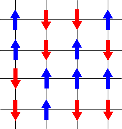
(a)

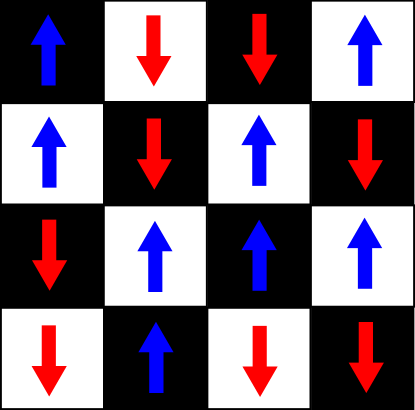
(b)

Figure 1: The checkerboard method marks each spin of a lattice (a) with a color from a checkerboard pattern (b). All spins marked with the same color are updated in parallel.

It is important to note that the order of the neighborhood of interacting spins is an important aspect of the spin models because it determines the nature of the interactions between spins. In the original Ising model, the interactions between spins are limited to the nearest neighbors, for which the checkerboard method is the most efficient. However, this method is not limited only to this type of neighborhood, and can be used at any order of spins interaction, as long as the central site is marked with one color and its neighbors are marked with another color.

III Methods

One of main challenges of implementing differentiable programming is translating an algorithm in a way that DP could be advantageous. The Metropolis-Hastings algorithm is typically implemented using either functional or object-oriented programming paradigms. Translating this algorithm to differentiable programming requires some modifications to how the algorithm is formulated and implemented.

In traditional functional or object-oriented programming, the Metropolis algorithm is typically implemented using a sequence of discrete steps. These steps involve updating the spin variables, computing the energy of the system, and then accepting or rejecting the proposed configuration based on the Metropolis acceptance criterion.

Within the modern differentiable programming frameworks, we can express an array of elements as a batched tensor with sizes up to five dimensions. For instance, deep learning applied in computer vision usually uses an array of images that can be represented as a tensor with size $[B,C,H,W]$, with $B$ the batch dimension, $C$ the channel dimension and $H,W$ the height and width of the images respectively.

Since the 4-dimensional format of $[B,C,H,W]$ is compatible with many modern deep learning frameworks, it makes easy to apply deep learning techniques to two-dimensional spin lattices. This can be particularly advantageous when using differentiable programming to simulate spin models, as it allows for seamless integration with existing deep learning tools and techniques. Additionally, the use of a batch dimension allows for efficient processing of multiple spin lattices simultaneously. This can be useful when simulating large-scale spin models, as it enables parallel processing of multiple samples or multiple temperatures at the same time.

III.1 Ising model

The Ising model consists of two states, called spins, which physically represent the magnetic moment of materials. They can be in a up state $(\sigma=+1)$ or down state $(\sigma=-1)$. This model has a phase transition in certain lattice geometries, where a change on the behavior of physical quantities, such as the collective magnetic field, occurs. For example, on a 2D square lattice with $J<0$, the Ising model predicts a change from a paramagnetic phase, characterized by a random mixture of spins, to a ferromagnetic phase, characterized by a alignment of the spins. The Hamiltonian describes the energy of the system is:

$$\mathcal{H}=\sum_{i,j}J_{ij}\sigma_{i}\sigma_{j}+\sum_{i}B_{i}\sigma_{i},$$ (1)

with $J_{i,j}$ being the interaction strength between spins $\sigma_{i}$ and $\sigma_{j}$, and $B_{i}$ an external magnetic field on spin $\sigma_{i}$.

The modified Monte Carlo simulation of the Ising model using the Metropolis-Hastings algorithm requires a convolution operation to calculate the system’s Hamiltonian. This convolution depends on two topological conditions of the system: its dimension and connectivity. The dimension of the system directly determines the dimension of the convolution, with a 1D convolution used for one-dimensional spin networks, 2D convolution for square or triangular networks, and 3D convolution for cubic networks, and so on. The connectivity of the system, which describes how the sites are connected, determines the shape of the convolution kernel.

For example, consider a square network with first-neighbor interactions. Each site is connected to its four nearest neighbors, which are located above, below, to the right and to the left of it. In this case, the kernel used in the convolution would have a size of $3\times 3$, with values of $1$ in the positions corresponding to the neighboring sites and $0$ everywhere else, including the center (to prevent the value of the site itself from being counted).

By using this modified algorithm, it becomes possible to efficiently simulate the behavior of the Ising model for systems with large numbers of particles. The convolution operation provides an efficient way to calculate the system’s Hamiltonian, which is a crucial step in the Metropolis-Hastings algorithm.

The kernel of the convolution states the geometry of the lattice. For the square lattice, the kernel is:

$$K=\begin{bmatrix}0&1&0\\ 1&0&1\\ 0&1&0\end{bmatrix}$$ (2)

Thus, for each spin, the energy is obtained by the top, down,left and right neighbors, which corresponds to the square lattice interaction. Note that the kernel shape doesn’t necessarily have to be square, as long as it accounts for the geometric shape of the network. The shape of the kernel is important because it determines the specific features that are extracted from the network. For example, if the kernel is square, it may extract different features compared to a triangular or hexagonal kernel. However, as long as the kernel accounts for the geometric shape of the network, it can be any shape that is suitable for the particular analysis.

For lattices with other connectivity, for instance, the triangular lattice, a transformation is necessary to convert the triangular lattice into a square lattice so that a square kernel can be used. This transformation involves adding null spins to the left and right of the central spin, which effectively creates a rectangular shape for the kernel:

$$K=\begin{bmatrix}0&1&0&1&0\\ 1&0&0&0&1\\ 0&1&0&1&0\end{bmatrix},\hskip 10.0pt K=\begin{bmatrix}1&0&1\\ 0&0&0\\ 0&1&0\end{bmatrix}.$$ (3)

By applying the convolution operation to the lattice using this rectangular kernel, the algorithm produces a map that is associated with the sum of the first neighbors’ spins for each site. This map can be used to obtain the Hamiltonian of each site.

The output of the convolution operation applied to the network is a map that is associated with the sum of the first neighbors’ spins. This map provides information about the local interactions between spins in the lattice and is an important input for further analysis. By multiplying the map produced by the convolution operation with the spin network itself, the Hamiltonian of each site in the lattice can be obtained, as described in algorithm 1.

Algorithm 1 Differentiable programming Metropolis-Hasting

1:initialize 2D square lattice $\mathbf{state}=\mathbf{(B,1,N,N)}$ from a random distribution

2:while $\mbox{MC step}\leq T$ do

3:     Propose new random states $\mathbf{state^{\prime}}$ for the lattice;

4:     Apply 2D convolution with kernel selected from the model and connectivity in both states;

5:     Multiply the result of the convolution to its respective state;

6:     Apply checkerboard algorithm;

7:     Evaluate the variation in energy $\Delta E$ for each site with same checkerboard color;

8:     if $\Delta E\leq 0$ then

9:         Accept the change

10:     else

11:         Accept the change with probability $p=e^{-\beta\Delta\mathcal{H}}$

12:     end if

13:end while

III.2 Potts model

The Potts model Wu (1982b) is a lattice model that describes the behavior of a system of interacting spins, which can take on more than two possible states. Unlike the Ising model, which has spins that can only take on two states (up or down), the Potts model allows spins to take on $q$ different states, with $q$ being any integer greater than or equal to $2$. Each spin is represented by an integer variable $\sigma_{i}$ that can take on values from 0 to $q-1$.

The Hamiltonian for the Potts model is given by

$$\mathcal{H}=\sum_{i,j}J_{i,j}\delta(\sigma_{i},\sigma_{j})+\sum_{i}B_{i}\sigma_{i},$$ (4)

where the first term represents the interactions between neighboring spins and the second term represents the effect of an external magnetic field on each spin. The coupling between spins $J_{i,j}$ is a constant that depends on the interaction between spins $i$ and $j$. The Kronecker delta function $\delta(\sigma_{i},\sigma_{j})$ equals $1$ if $\sigma_{i}=\sigma_{j}$ and $0$ otherwise.

The Potts model has applications in various fields, such as statistical physics, materials science, and computer science. It can be used to model phase transitions Tanaka et al. (2011), magnetic ordering Chang and Shrock (2023), and coloring of graphs Davies (2018). The model has also been used in image processing and computer vision, where it can be used to cluster pixels based on their colors or textures Portela et al. (2013).

To simulate the Potts model, the Metropolis-Hastings algorithm can be used, similarly to is done for the Ising model. The simulation involves selecting a random spin and attempting to change its state to a new value using a trial move. If the energy change resulting from the trial move is negative, the move is accepted. If the energy change is positive, the move is accepted with a probability given by a acceptance probability. In the Potts model, a spin flip is not well-defined since the spin can take on more than two states. Instead, a random spin is chosen to undergo a state change, with the new state being chosen from the $q-1$ possible values that are different from the current state.

The differentiable programming Metropolis-Hastings algorithm in the Potts model follows a structure similar to that used for the Ising model, by utilizing convolution. However, the main difference between the two models lies in the Potts model’s convolution, which employs more than one convolutional filter, each with its own kernel. The number of kernels is determined by the geometric properties of the system of interest, and each kernel accounts for a central site neighbor.

For instance, in the case of a square lattice with first neighbor interaction, four kernels are required, as shown below:

$$K=\begin{bmatrix}0&1&0\\ 0&0&0\\ 0&0&0\end{bmatrix},\ K=\begin{bmatrix}0&0&0\\ 1&0&0\\ 0&0&0\end{bmatrix},\ K=\begin{bmatrix}0&0&0\\ 0&0&1\\ 0&0&0\end{bmatrix},\ K=\begin{bmatrix}0&0&0\\ 0&0&0\\ 0&1&0\end{bmatrix}.$$ (5)

The separation of the kernels into four distinct filters is due to the Kronecker delta, which requires that each interaction with a neighbor to be accounted for separately. This contrasts with the Ising model, where the sum of neighboring spins multiplied by the central spin is sufficient.

After applying convolution with the four filters, four maps are generated for each site. To obtain the Hamiltonian of the system, the difference between each map and the spin configuration is computed. If the spins are equal, the map’s value at that position is set to zero; otherwise, the value of 1 is assigned. The resulting four maps are summed to generate a single map, which, multiplied by the spin configuration of the lattice, represents the Hamiltonian of the system, which can then be used to compute various variables of interest.

III.3 Cellular Potts model

Cells arrange themselves spatially during morphogenesis, wound healing, or regeneration to build new tissues or restore damaged ones. There are a number of intercellular methods of interaction that are used to carry out these functions. Cell-cell adhesion is a key process that can direct cell motion in a manner similar to the separation of immiscible liquids due to interfacial tensions, where the liquid phases are associated with various cell types (e.g. cells of retina, liver, etc). A well known phenomenon is the spontaneous separation of randomly mixed cell types which is known as cell sorting Foty and Steinberg (2013). The Cellular Potts Model (CPM), developed by Graner and Glazier, takes into account cellular adhesion to explain cell sorting and is frequently used to describe cellular processes Glazier and Graner (1993).

In the two dimensional CPM, cells are represented as identical spin domains on a lattice. Each spin $\sigma$ has a position $\vec{x}$ and a type index $\tau\left(\sigma\right)$ (a second quantum number). The hamiltonian (6), which represents cell-cell adhesion and interaction with cell culture media (a source of nutrients), describes the dynamics. Cell area is controlled by a second quadratic energy constraint. The medium around the cell aggregate is represented mathematically as a (big) cell with unconstrained area. The hamiltonian is written as follows

$$\mathcal{H}=\frac{1}{2}\sum_{\vec{x}}\sum_{\vec{y}}^{N_{max}}J_{\tau(\sigma(\vec{x})),\tau(\sigma(\vec{y}))}\left(1-\delta_{\sigma(\vec{x}),\sigma(\vec{y})}\right)+\lambda\sum_{\sigma}(a_{\sigma}-A_{\sigma})^{2}\,\,\,,$$ (6)

where $J_{\tau(\sigma(\vec{x})),\tau(\sigma(\vec{y}))}$ are the cell-cell or cell-medium adhesion energies that depend on the cell type $\tau$, $\delta$ is the Kronecker’s delta function, $\lambda$ a Lagrange multiplier that controls cell area compressibility, $a_{\sigma}$ the cell area and $A_{\sigma}$ the cell target area. By specifying energy only at the cell-cell contact, the Hamiltonian’s first term (6) mimics cellular adhesion.

The CPM simulates cell motion driven by the cytoskeleton by performing attempts to change the value in a given lattice position for another in its vicinity, what causes domain boundary motion representing cellular membrane motion. By selecting a target spin ($\sigma(\vec{x})$) and a neighbor spin ($\sigma(\vec{y})$) at random from the cell lattice, the system dynamic occurs. The change in the target spin value for its neighbor’s spin value is then decided utilizing the aforementioned algorithm 1.

When implementing the cellular Potts model, using simple convolutions like in previous models is not sufficient because the interaction between spins, denoted by $J$, is no longer constant. Instead, it depends on the spin value and the type of cell. To address this, differentiable programming techniques are used, and one operation that is particularly useful for implementing convolutions is called unfolding Lista (2017).

Unfolding involves dividing a set of elements, such as a vector, matrix, or other multidimensional set, into smaller, equally sized parts called “patches”. The size of these patches depends on the parameters of the convolution, such as the stride and padding. For example, if we apply unfolding with padding 0, stride 4, and a kernel of size $4\times 4$ to an 8x8 pixel image, we would obtain four parts of the image, each with a size of $4\times 4$ pixels.

The cellular Potts model involves interactions between neighboring cells, and the properties of the unfolding depend on the nature of these interactions. Typically, an odd number is used to account for the central cell. For instance, if first-neighbor interactions are considered, the kernel size will be $3\times D$, where $D$ is the dimension of the system. The stride will be set to 1 to compute the energy value for each cell, while the padding will depend on the boundary conditions specified, as in the Ising and Potts models. If second-neighbor interactions are considered, the kernel will be larger, with a size of $5\times 5$ to account for more distant cells.

Once the unfolding operation and padding are applied, the next step is to copy the central spin value of each patch to the same size as the patches. This allows us to obtain a consistent representation of the spin values across the entire grid. Finally, once the central sites have been copied, each patch is compared to its corresponding copy of the central sites, element by element. During this comparison, the interaction values are assigned based on the spin value and cell type. After the comparison, the energy map per site of the system is generated by summing the values of each compared patch.

IV Results

The differentiable programming Ising-Hastings algorithm was employed to simulate all models discussed above. The simulations were carried out using a computing system comprising an Intel Core i7-11800H CPU, a Nvidia GeForce RTX 3060 GPU, and a TPU which was utilized through Google Colab Bisong (2019). For the Ising and Potts models, we simulate lattices with different sizes, with $J=-1$ and first-order neighbor interactions.

The cellular Potts model considers the simulation of cell behavior. In this simulation, three cell types were chosen: light cells, dark cells, and the medium, following the original work of 1993 Glazier and Graner (1993). Additionally, 37 different spin values were chosen, with a value of 0 representing the medium, where each spin value leads to the formation of a unique cell. The chosen interaction energies are presented in table 1, and these interactions are symmetric (the interaction value is the same if site A interacts with site B or B with A). The interaction uses the Moore neighborhood with second neighbors. The temperature was set to $k_{B}T=8$.

Interaction	$J_{\tau,\tau^{\prime}}$
Medium-Medium	$0$
Medium-Dark	$16$
Medium-Light	$16$
Light-Light	$2$
Dark-Dark	$14$
Light-Dark	$11$

Table 1: The interaction values $J$ depends on the cell type, for the cellular Potts model.

IV.1 Ising model

Figure 2 shows snapshots of the square lattice Ising model for three different temperatures. The temperature of the system determines the probability of the spins flipping between up and down states. At low temperatures, the spins tend to align with their neighbors, forming large clusters that grow in size as the temperature decreases. This is due to the reduction in thermal energy, which favors the alignment of neighboring spins. These large clusters are known as domains, and they play an important role in the behavior of the system.

As the critical temperature is approached, the influence of long-range interactions between spins becomes more pronounced, leading to a change in the collective behavior of the system. At this temperature, the system undergoes a phase transition, characterized by the emergence of long-range correlations and critical fluctuations. This is a critical point where the properties of the system change abruptly.

Above the critical temperature, at hight temperatures, the domains disappear, and the system becomes disordered, with no long-range correlations. Thermal fluctuations dominate the behavior of the lattice, leading to random changes in the spin values. As the temperature increases, the magnetic spins become increasingly disordered, leading to a loss of magnetization in the system.

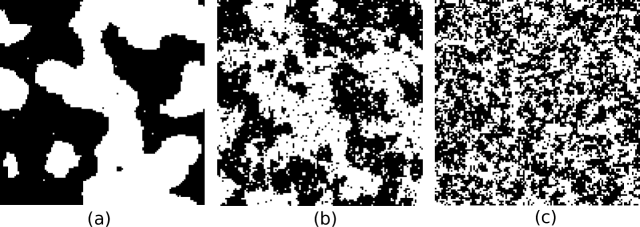
Figure 2: Lattice configurations for three different temperatures of the Ising model. (a) $T<Tc$, (b) $T\approx Tc$, (c) $T>Tc$.

The results for three different hardware are presented in Figure 3. Simulations run on CPU show consistent runtimes across varying batch and lattice sizes. On the other hand, GPU simulations outperform CPU by nearly 100 times in terms of speed. Notably, TPU simulations demonstrate a significant advantage in runtime as the lattice size and batch size increases, with a speedup of 10x compared to GPU simulations.

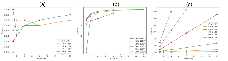
Figure 3: Flips per nanosecond for different lattice and batch sizes. (a) Simulation on CPU, (b) GPU and (c) TPU.

IV.2 Potts model

In the case of the Potts model, the spins can take on several different states, resulting in a more complex system with a richer set of behaviors. As the temperature is lowered, the spins tend to align themselves to form distinct clusters, as shown in figure 4. This behavior is reminiscent of ferromagnetism, in which the magnetic moments of individual atoms align themselves in the same direction.

On the other hand, at higher temperatures, the spins in the Potts model become more disordered and exhibit more frequent state changes, resulting in a more random and unpredictable system. This behavior is similar to what is observed in the Ising model, where at high temperatures, the magnetic moments of individual atoms become more disordered and fluctuate rapidly.

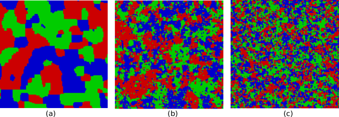
Figure 4: Lattice configurations for three different temperature of the Potts model with $q=3$. Each color represents a spin state. (a) $T<Tc$, (b) $T\approx Tc$, (c) $T>Tc$.

The Potts model has the same computational complexity as the Ising model, thus, the time required to flip the spins is similar for both models. This is because flipping the spin of a single site in the Potts model requires the calculation of the energy difference between the current and proposed spin states, just as in the Ising model. However, in the Potts model, the energy difference depends on the number of neighboring spins that have different states, which leads to a more complex calculation than in the Ising model.

Despite this additional complexity, the computational cost of flipping the spins in the Potts model is still comparable to that of the Ising model. The number of neighboring spins is typically small compared to the total number of spins in the system. As a result, simulations of the Potts model can be performed with similar computational resources and time requirements as those for the Ising model.

IV.3 Cellular Potts model

The evolution of a cell aggregate can be observed in Figure 5, where snapshots of the system’s states are shown with increasing Monte Carlo steps. Starting from an arbitrary aggregate of square-shaped cells, the system undergoes a process that aims to minimize the number of energy-costly boundaries, resulting in the sorting of the two cell types.

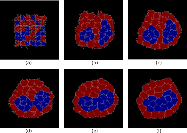
Figure 5: Cellular Potts Model simulation. Each figure is snapshot from different steps of the simulation. The cells spontaneously reorder themselves into clusters of same type as the the number of Monte Carlo steps increases.

The boundary length between each cell type can be observed in Figure 6, showing the evolution of the system. As the simulation progresses, we observe the interface between the blue cells and the medium vanishing, while the boundary length between red cells with medium and red cells with blue cells approaches a minimum value.

The simulation’s results suggest that the energy constraints in the system drive the behavior of the cell aggregate towards a more stable configuration, where the number of energy-costly boundaries is minimized. The decreasing boundary length between the different cell types indicates that the cells are actively interacting with each other, eventually sorting themselves into more cohesive groups.

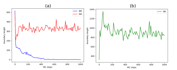
Figure 6: Boundary length between different cells types. (a) Blue cells and medium (blue line) and red cells and medium (red line). (b) Blue and red cells: we observe that the boundary length between blue cells and the medium goes to zero as the red cells surround the blue cells.

The phenomenon of cell sorting is a well-known example of self-organization in biological systems. It has been studied extensively both experimentally and theoretically, and its underlying mechanisms are thought to involve a complex interplay of various physical and biochemical processes Durand (2021); Nakajima and Ishihara (2011).

One of the key factors that influence cell sorting is the interaction between cells and their surrounding environment. Some studies have shown that the CPM can be used to model not only cell sorting but also other cellular behaviors such as movement Guisoni et al. (2018) and migration Scianna and Preziosi (2021). By varying the values of interaction $J$ between cells, it is possible to simulate different scenarios and study their effects on cellular behavior. Since the difference among these different phenomena are only in the interaction values, the computational cost of simulating the model with differentiable programming remains the same.

V Conclusions

In this paper, we have presented a novel approach for simulating three different spin models using differentiable programming. Our method applies convolution on the spins, similar to how convolution is applied to images in computer vision, which allows us to calculate the Hamiltonian of the system with high accuracy and efficiency. In addition, we made use of the checkerboard algorithm to parallelize the calculation of the energy of each spin. This algorithm involves dividing the spins into two sets, with each set updating alternately, such that neighboring spins are updated on different iterations. By doing so, we can parallelize the calculation of the energy of each spin, further improving the efficiency of our approach.

The use of the checkerboard algorithm in conjunction with our approach provides a significant boost in performance, enabling us to simulate spin models with high speed due to the parallelization. We believe that this approach could be widely applicable in many scientific applications that require fast and accurate simulations of complex physical systems.

The use of differentiable programming in this context is particularly useful, as it enables us to leverage the strengths of deep learning techniques for scientific simulations. We demonstrated the effectiveness of our approach by implementing it in PyTorch, which provides easy adaptability to run on GPUs and TPUs. Our experiments show that our method provides a significant speed-up in simulating spin models, without sacrificing accuracy. Moreover, by making use of the batch dimension, we were able to parallelize the simulation even further, leading to an additional increase in performance.

One important point to note is that our method is not fully differentiable, and we do not use the derivatives for computation. However, this does not detract from the value of our approach. In fact, our method is designed to maximize performance and speed, rather than optimizing for the use of derivatives. Therefore, we gain the advantage of a significant speed-up in simulating spin models, which can be critical in many scientific applications.

Our work provides a promising direction for future research in this field, as it opens up new opportunities for accelerating simulations and improving our understanding of complex physical phenomena. We anticipate that our method could have a wide range of applications in the future, especially in cases where speed and scalability are essential. By leveraging the power of differentiable programming, we can enable faster simulations and deeper insights into the behavior of physical systems.

Data availability. The data and code that support the findings of this study are available at https://github.com/tiago939/dp_monte_carlo.

References

- Khan et al. (2018) S. Khan, H. Rahmani, S. A. A. Shah, and M. Bennamoun, Synthesis Lectures on Computer Vision 8, 1–207 (2018).
- Bing et al. (2018) Z. Bing, C. Meschede, F. Röhrbein, K. Huang, and A. C. Knoll, Frontiers in Neurorobotics 12 (2018), ISSN 1662-5218, URL https://www.frontiersin.org/articles/10.3389/fnbot.2018.00035.
- Jumper et al. (2021) J. Jumper, R. Evans, A. Pritzel, T. Green, M. Figurnov, O. Ronneberger, K. Tunyasuvunakool, R. Bates, A. Žídek, A. Potapenko, et al., Nature 596, 583 (2021), ISSN 1476-4687, URL https://www.nature.com/articles/s41586-021-03819-2.
- Gaunt et al. (2017) A. L. Gaunt, M. Brockschmidt, N. Kushman, and D. Tarlow, in Proceedings of the 34th International Conference on Machine Learning, edited by D. Precup and Y. W. Teh (PMLR, 2017), vol. 70 of Proceedings of Machine Learning Research, pp. 1213–1222, URL https://proceedings.mlr.press/v70/gaunt17a.html.
- Rumelhart et al. (1986) D. E. Rumelhart, G. E. Hinton, and R. J. Williams, Nature 323, 533–536 (1986).
- Paszke et al. (2019) A. Paszke, S. Gross, F. Massa, A. Lerer, J. Bradbury, G. Chanan, T. Killeen, Z. Lin, N. Gimelshein, L. Antiga, et al., in Advances in Neural Information Processing Systems 32 (Curran Associates, Inc., 2019), pp. 8024–8035, URL http://papers.neurips.cc/paper/9015-pytorch-an-imperative-style-high-performance-deep-learning-library.pdf.
- Abadi et al. (2016) M. Abadi, P. Barham, J. Chen, Z. Chen, A. Davis, J. Dean, M. Devin, S. Ghemawat, G. Irving, M. Isard, et al., in 12th USENIX Symposium on Operating Systems Design and Implementation (OSDI 16) (2016), pp. 265–283.
- Bradbury et al. (2018) J. Bradbury, R. Frostig, P. Hawkins, M. J. Johnson, C. Leary, D. Maclaurin, G. Necula, A. Paszke, J. VanderPlas, S. Wanderman-Milne, et al., JAX: composable transformations of Python+NumPy programs (2018), URL http://github.com/google/jax.
- Jouppi et al. (2017) N. P. Jouppi, C. Young, N. Patil, D. Patterson, G. Agrawal, R. Bajwa, S. Bates, S. Bhatia, N. Boden, A. Borchers, et al. (2017), URL https://arxiv.org/pdf/1704.04760.pdf.
- Eshraghian et al. (2021) J. K. Eshraghian, M. Ward, E. Neftci, X. Wang, G. Lenz, G. Dwivedi, M. Bennamoun, D. S. Jeong, and W. D. Lu, arXiv preprint arXiv:2109.12894 (2021).
- Bergholm et al. (2022) V. Bergholm, J. Izaac, M. Schuld, C. Gogolin, S. Ahmed, V. Ajith, M. S. Alam, G. Alonso-Linaje, B. AkashNarayanan, A. Asadi, et al., PennyLane: Automatic differentiation of hybrid quantum-classical computations (2022), arXiv:1811.04968 [physics, physics:quant-ph], URL http://arxiv.org/abs/1811.04968.
- Baydin et al. (2018) A. G. Baydin, B. A. Pearlmutter, A. A. Radul, and J. M. Siskind, The Journal of Machine Learning Research 18, 1 (2018).
- BRUSH (1967) S. G. BRUSH, Rev. Mod. Phys. 39, 883 (1967), URL https://link.aps.org/doi/10.1103/RevModPhys.39.883.
- MIYASHITA (2010) S. MIYASHITA, Proceedings of the Japan Academy. Series B, Physical and Biological Sciences 86, 643 (2010), ISSN 0386-2208, URL https://www.ncbi.nlm.nih.gov/pmc/articles/PMC3066537/.
- Rens and Edelstein-Keshet (2019) E. G. Rens and L. Edelstein-Keshet, PLoS Computational Biology 15, e1007459 (2019), ISSN 1553-734X, URL https://www.ncbi.nlm.nih.gov/pmc/articles/PMC6927661/.
- Kinzel (1985) W. Kinzel, in Complex Systems — Operational Approaches in Neurobiology, Physics, and Computers, edited by H. Haken (Springer, Berlin, Heidelberg, 1985), Springer Series in Synergetics, pp. 107–115, ISBN 9783642707957.
- Ising (1925) E. Ising, Z. Physik 31, 253 (1925).
- Wu (1982a) F. Y. Wu, Rev. Mod. Phys. 54, 235–268 (1982a).
- Szabó and Merks (2013) A. Szabó and R. M. Merks, Frontiers in Oncology 3, 87 (2013).
- Hirashima et al. (2017) T. Hirashima, E. G. Rens, and R. M. H. Merks, Development, Growth & Differentiation 59, 329 (2017), ISSN 0012-1592, 1440-169X, URL https://onlinelibrary.wiley.com/doi/10.1111/dgd.12358.
- Chen et al. (2007) N. Chen, J. A. Glazier, J. A. Izaguirre, and M. S. Alber, Computer Physics Communications 176, 670 (2007), ISSN 0010-4655, URL https://www.sciencedirect.com/science/article/pii/S0010465507002044.
- Durand (2021) M. Durand, PLoS Computational Biology 17, e1008576 (2021), ISSN 1553-734X, URL https://www.ncbi.nlm.nih.gov/pmc/articles/PMC8389523/.
- Szabó and Merks (2013) A. Szabó and R. M. H. Merks, Frontiers in Oncology 3, 87 (2013), ISSN 2234-943X, URL https://www.ncbi.nlm.nih.gov/pmc/articles/PMC3627127/.
- Metzcar et al. (2019) J. Metzcar, Y. Wang, R. Heiland, and P. Macklin, JCO Clinical Cancer Informatics pp. 1–13 (2019), pMID: 30715927, eprint https://doi.org/10.1200/CCI.18.00069, URL https://doi.org/10.1200/CCI.18.00069.
- Katzgraber (2009) H. G. Katzgraber, arXiv.0905.1629 (2009).
- Schneider and Stoll (1974) T. Schneider and E. Stoll, Phys. Rev. B 10, 959 (1974), URL https://link.aps.org/doi/10.1103/PhysRevB.10.959.
- Kotze (2008) J. Kotze, Introduction to monte carlo methods for an ising model of a ferromagnet (2008), URL https://arxiv.org/abs/0803.0217.
- Gould and Tobochnik (1989) H. Gould and J. Tobochnik, Computers in Physics 3, 82 (1989), ISSN 0894-1866, URL https://aip.scitation.org/doi/abs/10.1063/1.4822858.
- Acharyya (1997) M. Acharyya, Phys. Rev. E 56, 2407 (1997), URL https://link.aps.org/doi/10.1103/PhysRevE.56.2407.
- Shekaari and Jafari (2021) A. Shekaari and M. Jafari, Theory and simulation of the ising model (2021), URL https://arxiv.org/abs/2105.00841.
- Scroggs et al. (2022) M. W. Scroggs, J. S. Dokken, C. N. Richardson, and G. N. Wells, ACM Transactions on Mathematical Software (2022), to appear.
- Rathgeber et al. (2016) F. Rathgeber, D. A. Ham, L. Mitchell, M. Lange, F. Luporini, A. T. T. Mcrae, G.-T. Bercea, G. R. Markall, and P. H. J. Kelly, ACM Transactions on Mathematical Software 43, 24:1 (2016), ISSN 0098-3500, URL https://dl.acm.org/doi/10.1145/2998441.
- Jin et al. (2020) W. Jin, Z. Wang, Z. Yang, and S. Mou, in Advances in Neural Information Processing Systems, edited by H. Larochelle, M. Ranzato, R. Hadsell, M. Balcan, and H. Lin (Curran Associates, Inc., 2020), vol. 33, pp. 7979–7992, URL https://proceedings.neurips.cc/paper_files/paper/2020/file/5a7b238ba0f6502e5d6be14424b20ded-Paper.pdf.
- Hu et al. (2021) Y. Hu, Y. Jin, X. Wu, and J. Chen, in 2021 International Conference on Electromagnetics in Advanced Applications (ICEAA) (2021), pp. 216–221.
- Grinis (2022) R. Grinis, Journal of Experimental and Theoretical Physics 134, 150 (2022), URL https://doi.org/10.1134%2Fs1063776122020042.
- Rackauckas et al. (2021) C. Rackauckas, A. Edelman, K. Fischer, M. Innes, E. Saba, V. Shah, and W. Tebbutt (2021).
- Thuerey et al. (2021) N. Thuerey, P. Holl, M. Mueller, P. Schnell, F. Trost, and K. Um, Physics-based Deep Learning (WWW, 2021), URL https://physicsbaseddeeplearning.org.
- Hu et al. (2020) Y. Hu, L. Anderson, T.-M. Li, Q. Sun, N. Carr, J. Ragan-Kelley, and F. Durand, ICLR (2020).
- Takahashi et al. (2021) T. Takahashi, J. Liang, Y.-L. Qiao, and M. C. Lin, in AAAI (2021).
- Fan and Wang (2023) X. Fan and J.-X. Wang, Differentiable hybrid neural modeling for fluid-structure interaction (2023), eprint 2303.12971.
- Bezgin et al. (2023) D. A. Bezgin, A. B. Buhendwa, and N. A. Adams, Computer Physics Communications 282, 108527 (2023), ISSN 0010-4655, URL https://www.sciencedirect.com/science/article/pii/S0010465522002466.
- Efthymiou et al. (2019) S. Efthymiou, M. J. S. Beach, and R. G. Melko, Physical Review B 99, 075113 (2019), ISSN 2469-9950, 2469-9969, arXiv:1810.02372 [cond-mat], URL http://arxiv.org/abs/1810.02372.
- Liu et al. (2017) Z. Liu, S. P. Rodrigues, and W. Cai, Simulating the Ising Model with a Deep Convolutional Generative Adversarial Network (2017), arXiv:1710.04987 [cond-mat], URL http://arxiv.org/abs/1710.04987.
- Yu and Yang (2014) C. Yu and B. Yang, in 2014 11th International Joint Conference on Computer Science and Software Engineering (JCSSE) (2014), pp. 117–122.
- Christley et al. (2010) S. Christley, B. Lee, X. Dai, and Q. Nie, BMC Systems Biology 4, 107 (2010), ISSN 1752-0509, URL https://www.ncbi.nlm.nih.gov/pmc/articles/PMC2936904/.
- Tomeu and Salguero (2020) A. J. Tomeu and A. G. Salguero, Journal of Integrative Bioinformatics 17, 20190070 (2020), URL https://doi.org/10.1515/jib-2019-0070.
- Berghoff et al. (2020) M. Berghoff, J. Rosenbauer, F. Hoffmann, and A. Schug, BMC Bioinformatics 21, 436 (2020), ISSN 1471-2105, URL https://doi.org/10.1186/s12859-020-03728-7.
- Ghaemi and Shahrokhi (2006) M. Ghaemi and A. Shahrokhi, Combination of The Cellular Potts Model and Lattice Gas Cellular Automata For Simulating The Avascular Cancer Growth (2006), arXiv:nlin/0611025, URL http://arxiv.org/abs/nlin/0611025.
- Geman and Geman (1984) S. Geman and D. Geman, IEEE Transactions on Pattern Analysis and Machine Intelligence PAMI-6, 721 (1984).
- Wolff (1989) U. Wolff, Phys. Rev. Lett. 62, 361 (1989), URL https://link.aps.org/doi/10.1103/PhysRevLett.62.361.
- Hastings (1970) W. K. Hastings, Biometrika 57, 97 (1970), ISSN 00063444.
- Preis et al. (2009) T. Preis, P. Virnau, W. Paul, and J. Schneider, Journal of Computational Physics 228, 4468 (2009).
- Wu (1982b) F. Y. Wu, Rev. Mod. Phys. 54, 235 (1982b), URL https://link.aps.org/doi/10.1103/RevModPhys.54.235.
- Tanaka et al. (2011) S. Tanaka, R. Tamura, and N. Kawashima, Journal of Physics: Conference Series 297, 012022 (2011), URL https://dx.doi.org/10.1088/1742-6596/297/1/012022.
- Chang and Shrock (2023) S.-C. Chang and R. Shrock, Physica A: Statistical Mechanics and its Applications 613, 128532 (2023), ISSN 0378-4371, URL https://www.sciencedirect.com/science/article/pii/S0378437123000870.
- Davies (2018) E. Davies, The Electronic Journal of Combinatorics 25 (2018), URL https://doi.org/10.37236%2F7743.
- Portela et al. (2013) N. M. Portela, G. D. Cavalcanti, and T. I. Ren, in 2013 IEEE 25th International Conference on Tools with Artificial Intelligence (2013), pp. 256–261.
- Foty and Steinberg (2013) R. Foty and M. S. Steinberg, Differential adhesion in model systems 2, 631 (2013).
- Glazier and Graner (1993) J. Glazier and F. Graner, Physical Review E 47, 2128–2154 (1993).
- Lista (2017) L. Lista, Convolution and Unfolding (2017), pp. 155–174, ISBN 978-3-319-62839-4.
- Bisong (2019) E. Bisong, Google Colaboratory (Apress, Berkeley, CA, 2019), pp. 59–64, ISBN 978-1-4842-4470-8, URL https://doi.org/10.1007/978-1-4842-4470-8_7.
- Nakajima and Ishihara (2011) A. Nakajima and S. Ishihara, New Journal of Physics 13, 033035 (2011), ISSN 1367-2630, URL https://dx.doi.org/10.1088/1367-2630/13/3/033035.
- Guisoni et al. (2018) N. Guisoni, K. I. Mazzitello, and L. Diambra, Frontiers in Physics 6 (2018), ISSN 2296-424X, URL https://www.frontiersin.org/articles/10.3389/fphy.2018.00061.
- Scianna and Preziosi (2021) M. Scianna and L. Preziosi, Axioms 10 (2021), ISSN 2075-1680, URL https://www.mdpi.com/2075-1680/10/1/32.