Minimizing Running Buffers for Tabletop Object Rearrangement: Complexity, Fast Algorithms, and Applications

Abstract

For rearranging objects on tabletops with overhand grasps, temporarily relocating objects to some buffer space may be necessary. This raises the natural question of how many simultaneous storage spaces, or “running buffers”, are required so that certain classes of tabletop rearrangement problems are feasible. In this work, we examine the problem for both labeled and unlabeled settings. On the structural side, we observe that finding the minimum number of running buffers (MRB) can be carried out on a dependency graph abstracted from a problem instance, and show that computing MRB is NP-hard. We then prove that under both labeled and unlabeled settings, even for uniform cylindrical objects, the number of required running buffers may grow unbounded as the number of objects to be rearranged increases. We further show that the bound for the unlabeled case is tight. On the algorithmic side, we develop effective exact algorithms for finding MRB for both labeled and unlabeled tabletop rearrangement problems, scalable to over a hundred objects under very high object density. More importantly, our algorithms also compute a sequence witnessing the computed MRB that can be used for solving object rearrangement tasks. Employing these algorithms, empirical evaluations reveal that random labeled and unlabeled instances, which more closely mimics real-world setups, generally have fairly small MRBs. Using real robot experiments, we demonstrate that the running buffer abstraction leads to state-of-the-art solutions for in-place rearrangement of many objects in tight, bounded workspace.

1 Introduction

In nearly all aspects of our daily lives, be it work-related, at home, or for play, objects are to be grasped and rearranged, e.g., tidying up a messy desk, cleaning the table after dinner, or solving a jigsaw puzzle. Similarly, many industrial and logistics applications require repetitive rearrangements of many objects, e.g., the sorting and packaging of products on conveyors with robots, and doing so efficiently is of critical importance to boost the competitiveness of the stakeholders.

However, even without the challenge of grasping, deciding the object manipulation order for optimizing a rearrangement task is non-trivial. To that end, [1] examined the problem of tabletop object rearrangement with overhand grasps (TORO), where objects may be picked up, moved around, and then placed at poses that are not in collision with other objects. An object that is picked up but cannot be directly placed at its goal is temporarily stored at a buffer. For example, for the setup given in Fig. 1, using a single manipulator, either the Coke or the Pepsi must be moved to a buffer before the task can be completed. They show that computing a pick-n-place sequence that minimizes the use of the total number of buffers is NP-hard and provide methods for computing that solution for low tens of objects.

\begin{overpic}[width=260.17464pt]{figures/toro-ex-2-eps-converted-to.pdf} \end{overpic}

Figure 1: A TORO instance where the three soda cans are to be rearranged from the left configuration to the right configuration.

In this study, we examine an arguably more practical objective function that minimizes the number of running buffers (RB) in solving a TORO instance. In other words, we seek rearrangement plans that minimize the maximum number of objects stored at buffers at any given moment, assuming that each object is moved to a temporary location at most once. We denote this quantity as MRB (minimum # of running buffers). The MRB objective is important because if the required MRB for solving a TORO instance exceeds the available buffer storage, which is limited in practice, then the instance is infeasible. It is also shown that the objective is conducive to computing high-quality solutions for solving TORO tasks. Therefore, the structural results and the algorithms that we present may be used not only for computing feasible and high-quality rearrangement plans but are also invaluable as a verification tool, e.g., to verify that a certain rearrangement setup will be able to solve most tasks for which it is designed to tackle.

Surrounding the goal of studying TORO under the MRB objective, this work brings the following contributions:

• We propose and carry out an initial study of solving TORO tasks with a focus on minimizing the number of running buffers (MRB). The MRB objective is a natural alternative to minimizing the total number of buffers [1], whereas both objectives may serve as proxies for the computation of high-quality tabletop rearrangement plans.

• On the structural side, in terms of computational complexity, we show that computing MRB is NP-hard on arbitrary dependency graphs, which encodes the combinatorial information of TORO instances. We then further show that the NP-hardness of MRB computation extends to actual TORO instances.

• Continuing on the structural analysis of the MRB objective, we establish that for an $n$-object TORO instance where all objects are uniform cylinders, its MRB can be lower bounded by $\Omega(\sqrt{n})$, even when all objects are unlabeled. This implies that the same is true for the labeled setting. We then provide a matching algorithmic upper bound of $O(\sqrt{n})$ for the unlabeled setting.

• On the algorithmic side, we have developed multiple effective methods for solving various TORO tasks optimizing MRB, including a dynamic programming method for the labeled setting, a priority queue-based algorithm for the unlabeled setting, and a novel depth-first-search dynamic programming routine that readily scales to instances with over a hundred objects for both settings. Furthermore, we provide methods for computing plans with the minimum number of total buffers subject to the MRB constraints. These algorithms not only provide the optimal number of buffers but also provide a rearrangement plan that witnesses the optimal solution.

• Through extensive numerical evaluations and experimental validations, we confirm the effectiveness of MRB as a proper metric/proxy to optimize in computing high-quality solutions for TORO tasks. Specifically, MRB-based methods significantly outperform the previous state-of-the-art methods in many highly challenging TORO setups.

This paper builds on the conference version [2], with major additions; two of the most important ones are: (1) Many additional theoretical and algorithmic results are added; for both existing and new theorems, complete and expanded proofs are included, and (2) An application of MRB to carry out in-place tabletop rearrangement in a bounded workspace, with real robot experiment, is added. Part of this addition is based on [3] and with new and improved experiments (e.g., Fig. 2).

Figure 2: An in-place tabletop rearrangement instance with letter-shaped objects in a bounded workspace. The blue dominoes work as boundaries and do not fall during the execution.

Paper organization. The rest of the paper is organized as follows. We provide an overview of related literature in Sec. 2. In Sec. 3, we describe the MRB focused rearrangement problems and discuss the associated dependency graph structure. In Sec. 4, we establish some basic structural properties and show that computing MRB is computationally intractable. We proceed to establish lower and upper bounds on MRB for selected settings in Sec. 5 and describe our proposed algorithmic solutions in Sec. 6. In Sec. 7, we present an application of the MRB algorithms used in the extended scenario which allows internal running buffer s. Evaluation of simulations follows in Sec. 8. In Sec. 9, we set up a hardware platform to execute the rearrangement plans computed by our proposed algorithms. We discuss and conclude with Sec. 10.

2 Related Work

As a high utility capability, manipulation of objects in a bounded workspace has been extensively studied, with works devoted to perception/scene understanding [4, 5, 6, 7], task/rearrangement planning [8, 9, 10, 11, 12, 1, 13], manipulation [14, 15, 16, 17, 18, 19, 20, 21], as well as integrated, holistic approaches [22, 23, 24, 25, 26]. As object rearrangement problems often embed within them multi-robot motion planning problems, rearrangement inherits the PSPACE-hard complexity [27]. These problems remain NP-hard even without complex geometric constraints [28]. Considering rearrangement plan quality, e.g, minimizing the number of pick-n-places or the end-effector travel, is also computationally intractable [1].

For rearrangement tasks using mainly prehensile actions, the algorithmic studies of Navigation Among Movable Obstacles [8, 29] result in backtracking search methods that can effectively deal with monotone instances which restrict the robot to move each obstacle at most once. Via carefully calling monotone solvers, difficult non-monotone cases can be solved as well [11, 30]. [1] relates tabletop rearrangement problems to the Traveling Salesperson Problem [31] and the Feedback Vertex Set problem [32], both of which are NP-hard. Nevertheless, integer programming models could quickly compute high-quality solutions for practical sized ($\sim 20$ objects) problems. Focusing mainly on the unlabeled setting, bounds on the number of pick-n-places are provided for disk objects in [33]. In [13], a complete algorithm is developed that reasons about object retrieval, rearranging other objects as needed, with later work [34] considering plan optimality and sensor occlusion. While objectives in most problems focus on the number of motions, [35] seeks to minimize the space needed to carry out a rearrangement task for discs moving inside the workspace.

Non-prehensile rearrangement has also been extensively studied[36, 37], with object singulation as an early focus [38, 39, 40]. In this problem, a robot is tasked to separate a target object from surrounding obstacles with non-prehensile actions, e.g., pushing and poking, in order to provide room for performing grasping actions. An iterative search was employed in [37] for accomplishing a multitude of rearrangement tasks spanning singulating, separation, and sorting of identically shaped cubes. [41] combines Monte Carlo Tree Search with a deep policy network for separating many objects into coherent clusters within a bounded workspace, supporting non-convex objects. More recently, a bi-level planner is proposed [42], engaging both (non-prehensile) pushing and (prehensile) overhand grasping for sorting a large number of objects. Synergies between non-prehensile and prehensile actions have been explored for solving clutter removal tasks [43, 44] and more challenging object retrieval tasks [45, 46] using a minimum number of pushing and grasping actions.

On the structural side, a central object that we study is the dependency graph structure. Similar dependency structures were first introduced to multi-robot path planning problems to deal with path conflicts between agents [47, 48]. Subsequently, the structure was employed for reasoning about and solving challenging rearrangement problems [11, 49, 50, 51, 52]. The full labeled dependency graph, as induced by a rearrangement instance, is first introduced and studied in [1]. This current work introduces the unlabeled dependency graph. We observe that, in the labeled setting, through the dependency graph, the running buffer problems naturally connect to graph layout problems [53, 54, 55, 56, 57, 58], where an optimal linear ordering of graph vertices is sought. Graph layout problems find a vast number of important applications including VLSI design, scheduling [59], and so on. For the unlabeled setting, the dependency graph becomes a planar one for uniform objects with a round base. Rearrangement can be tackled through partitioning of the dependency graph using a vertex separator [60, 61, 62, 63]. For a survey on these topics, see [53].

3 Preliminaries

For TORO tasks where objects assume similar geometry, there are two natural practical settings depending on whether the objects are distinguishable, i.e., whether they are labeled or unlabeled. We describe external buffer formulations under these two distinct settings, and discuss the important dependency graph structure for both.

3.1 Labeled TORO with External Buffers

Consider a bounded workspace $\mathcal{W}\subset\mathbb{R}^{2}$ with a set of $n$ objects $\mathcal{O}=\{o_{1},\ldots,o_{n}\}$ placed inside it. All objects are assumed to be generalized cylinders with the same height. A feasible arrangement of these objects is a set of poses $\mathcal{A}=\{x_{1},\ldots,x_{n}\},x_{i}\in SE(2)$ in which no two objects collide. Let $\mathcal{A}_{1}=\{x_{1}^{s},\ldots,x_{n}^{s}\}$ and $\mathcal{A}_{2}=\{x_{1}^{g},\ldots,x_{n}^{g}\}$ be two feasible arrangements, a tabletop object rearrangement problem [1] seeks a plan using pick-n-place operations that move the objects from $\mathcal{A}_{1}$ to $\mathcal{A}_{2}$ (see Fig. 3(a) for an example with 7 uniform cylinders). In each pick-n-place operation, an object is grasped by a robot arm, lifted above all other objects, transferred to and lowered at a new pose $p\in SE(2)$ where the object will not be in collision with other objects, and then released. A pick-n-place operation can be formally represented as a 3-tuple $a=(i,x^{\prime},x^{\prime\prime})$, denoting that object $o_{i}$ is moved from pose $x^{\prime}$ to pose $x^{\prime\prime}$. A full rearrangement plan $P=(a_{1},a_{2},\ldots)$ is then an ordered sequence of pick-n-place operations.

\begin{overpic}[width=260.17464pt]{figures/problem_exp-eps-converted-to.pdf} \put(13.0,-4.0){{\small(a)}} \put(48.0,-4.0){{\small(b)}} \put(80.0,-4.0){{\small(c)}} \end{overpic}

Figure 3: A 7-object labeled instance with uniform cylinders; we will use this instance as a running example. (a) The unshaded discs (as projections of cylinders) represent the start arrangement $\mathcal{A}_{1}$ and the shaded discs represent the goal arrangement $\mathcal{A}_{2}$. (b) The corresponding labeled dependency graph. (c) The corresponding unlabeled dependency graph, which is bipartite and planar.

Depending on $\mathcal{A}_{1}$ and $\mathcal{A}_{2}$, it may not always be possible to directly transfer an object $o_{i}$ from $x_{i}^{s}$ to $x_{i}^{g}$ in a single pick-n-place operation, because $x_{i}^{g}$ may be occupied by other objects. This creates dependencies between objects. If object $o_{i}$ at pose $x^{g}_{i}$ intersects objects $o_{j}$ at pose $x^{s}_{j}$, we say $o_{i}$ depends on $o_{j}$. This suggests that object $o_{j}$ must be moved first before $o_{i}$ can be placed at its goal pose $x^{g}_{i}$.

It is possible to have circular dependencies. As an example, for the instance given in Fig. 3(a), objects $3$ and $5$ have dependencies on each other. In such cases, some object(s) must be temporarily moved to an intermediate pose to solve the rearrangement problem. Similar to [1], for most of this paper, we assume that external buffers outside of the workspace are used for intermediate poses, which avoids time-consuming geometric computations if the intermediate poses are to be placed within $\mathcal{W}$. During the execution of a rearrangement plan, there can be multiple objects that are stored at buffer locations. We call the buffers that are currently in use running buffers (RB). With the introduction of buffers, there are three types of pick-n-place operations: 1) pick an object at its start pose and place it at a buffer, 2) pick an object at its start pose and place it at its goal pose, and 3) pick an object from a buffer and place it at its goal pose. Notice that buffer poses are not important. Naturally, it is desirable to be able to solve a rearrangement problem with the least number of running buffers, giving rise to the labeled running buffer minimization problem.

Problem 1 (Labeled Running Buffer Minimization (LRBM)).

Given feasible arrangements $\mathcal{A}_{1}$ and $\mathcal{A}_{2}$, find a rearrangement plan $P$ that minimizes the maximum number of running buffers in use at any given time as the plan is executed.

In an LRBM instance, the set of all dependencies induced by $\mathcal{A}_{1}$ and $\mathcal{A}_{2}$ can be represented using a directed graph $G^{\,\ell}=(V,A)$, where each $v_{i}\in V$ corresponds to object $o_{i}$ and there is an arc $v_{i}\to v_{j}$ for $1\leq i,j\leq n,i\neq j$ if object $o_{i}$ depends on object $o_{j}$. We call $G^{\,\ell}$ a labeled dependency graph. The labeled dependency graph for Fig. 3(a) is given in Fig. 3(b). Based on the dependency graph $G^{\,\ell}$, we can immediately identify multiple circular dependencies in the graph, e.g., between objects $3$ and $5$, or among objects $7,2,6$ and $5$. The cycles form strongly connected components of $G^{\,\ell}$, which can be effectively computed [64]. Since moving objects to external buffers does not create additional dependencies, we have

Proposition 1.

$G^{\,\ell}$ fully captures the information needed to solve the tabletop rearrangement problem with external buffers moving objects from $\mathcal{A}_{1}$ to $\mathcal{A}_{2}$.

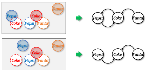
We use two examples to illustrate the relationships between TORO, its dependency graph, and external buffer-based solutions. First, for the example given in Fig. 1, the corresponding start/goal configurations are given in Fig. 4[top left]. The labeled dependency graph is given in Fig. 4[top right]. Because of the existence of cyclic dependencies between Coke and Pepsi, one of these two must be temporarily moved to a buffer. Suppose that Pepsi is moved to buffer. This changes the configuration and dependency graph as shown in the second row of Fig. 4. The TORO instance can then be readily solved. The complete solution sequence is $\langle Pepsi\to b,Coke\to g,Pepsi\to g,Fanta\to g\rangle$, where $b$ refers to a buffer and $g$ refers to the goal of the corresponding object.

Figure 4: Two configurations of the setup given in Fig. 1 and the corresponding dependency graphs.

For the example given in Fig. 3[a], its labeled dependency graph Fig. 3[b] shows two cycles ($2\leftrightarrow 7$ and $3\leftrightarrow 5$). One planning sequence for solving this can be derived that moves $2$ and $3$ to buffer: $\langle 1\to g,2\to b,3\to b,7\to g,4\to g,5\to g,6\to g,2\to g,3\to g\rangle$.

3.2 Unlabeled TORO with External Buffers

In the unlabeled setting, objects are interchangeable. That is, it does not matter which object goes to which goal. For example, in Fig. 3, object $5$ can move to the goal for object $6$. We call this version the unlabeled running buffer minimization (URBM) problem, which is intuitively easier. The plan for the unlabeled problem can be represented similarly as the labeled setting; we continue to use labels so that plans can be clearly represented but do not require matching labels for start and goal poses.

For the unlabeled setting, the dependency structure remains but appears in a different form. It is now an undirected bipartite graph. That is, $G^{\,u}=(V_{1}\cup V_{2},E)$ where each $v\in V_{1}$ (resp., $v\in V_{2}$) corresponds to a start (resp., goal) pose $p\in\mathcal{A}_{1}$ (resp., $p\in\mathcal{A}_{2}$). We denote the vertices representing the start and goal poses as start vertices and goal vertices, respectively. There is an edge between $v_{1}\in V_{1}$ and $v_{2}\in V_{2}$ if the objects at the corresponding poses overlap. The unlabeled dependency graph for Fig. 3(a) is illustrated in Fig. 3(c).

In practice, many TORO instances have objects with footprints that are uniform regular polygons (e.g., squares) or discs. In such settings, we can say something additional about the resulting unlabeled dependency graphs (the proofs of the two propositions below can be found in the appendix).

Proposition 2.

For unlabeled TORO where footprints of objects are uniform regular polygons, the maximum degree of the unlabeled dependency graph is upper bounded by 19.

Proposition 3.

For unlabeled TORO where footprints of objects are uniform discs, the dependency graph is a planar bipartite graph with a maximum degree of 5.

For either LRBM or URBM, the minimum required the number of running buffers is denoted as MRB, which can be computed based on the corresponding dependency graph.

4 Structural Analysis and NP-Hardness

The introduction of running buffers to tabletop rearrangement problems induces unique and interesting structures. We highlight some important structural properties of LRBM, including the comparison to minimizing the total number of buffers [1], the solutions of LRBM and linear arrangement [65] or linear ordering [66] of its dependency graph, and the hardness of computing MRB for TORO.

As will be established in this section, computing MRB solutions for TORO is intimately connected to finding a certain optimal linear ordering of vertices in the associated dependency graph. Because finding an optimal linear ordering is hard, it renders computing MRB solutions hard as well. This in turns limits the algorithmic solutions that one can secure for computing MRB solutions for TORO tasks.

4.1 Running Buffer versus Total Buffer

In solving TORO, running buffers are related to but different from the total number of buffers, as studied in [1]. It is shown the minimum number of total buffers for solving TORO is the same as the size of the minimum feedback vertex set (FVS) of the underlying dependency graph. An FVS is a set of vertices the removal of which leaves a graph acyclic. A TORO with an acyclic dependency graph can be solved without using any buffer because there are no cyclic dependencies between any pairs of objects. We denote the size of the minimum FVS as MFVS.

As a labeled TORO problem, the example from Fig. 1 has $\textsc{MFVS}=\textsc{MRB}=1$. For the example from Fig. 3(a)(b), $\textsc{MFVS}=2$ (an FVS set is $\{2,3\}$) and $\textsc{MRB}=2$.

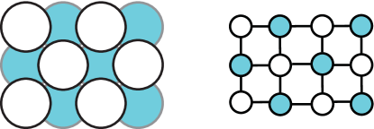
As an extreme example illustrating the difference between MRB and MFVS, consider a labeled dependency graph that is formed by $n$ copies of $2$-cycles, e.g., Fig. 5. The MFVS of the instance is $n$ because one vertex must be removed from each of the $n$ cycles to make the graph acyclic. On the other hand, the MRB is just $1$ because each cyclic dependency can be resolved independently from other cycles using a single external buffer. Therefore, whereas the total number of buffers used has more bearing on global solution optimality, MRB sheds more light on feasibility. Knowing the MRB tells us whether a certain number of external buffers will be sufficient for solving a class of rearrangement problems. This is critical for practical applications where the number of external buffers is generally limited to be a small constant. For example, in solving everyday rearrangement tasks, e.g., sorting things or retrieving items in the fridge, a human may attempt to temporarily hold multiple items, sometimes awkwardly. There is clearly a limit to the number of items that can be held simultaneously this way.

Figure 5: An instance with the labeled dependency graph formed by 3 copies of $2$-cycles. The MFVS is 3. On the other hand, the MRB is just $1$ for the problem. The example scales to have arbitrarily large MFVS with MRB remaining at $1$.

We give an example where the MRB and MFVS cannot always be optimized simultaneously, i.e., they form a Pareto front. For the setup in Fig. 6, the MFVS $\{7,9,10\}$ has size $3$ - it can be readily checked that deleting $\{7,9,10\}$ leaves the dependency graph acyclic. Using our algorithms, the MRB can be computed to be $2$ with the witness sequence being $1,10,8,4,5,3,6,7,2,9$, corresponding to the plan of $\langle 1\to g,10\to b,8\to g,4\to b,5\to g,3\to g,10\to g,6\to b,7\to g,6\to g,2\to b,9\to g,4\to g,2\to g\rangle$, where $b$ refers to a buffer and $g$ refers to the goal of the corresponding object. The RB reaches the maximum $2$ when $4$ and $6$ are moved to the buffer. However, in this case, the total number of buffers used is $4$: $2,4,6$, and $10$ are moved to buffers. This turns out to be the best we can do for this example, that is, if we are constrained by solutions with $\textsc{MRB}=2$, the total number of buffers that must be used is at least $4$ instead of the MFVS size of $3$.

We note that it is rarely the case that MFVS will be larger when the solution space is constrained to MRB solutions; for uniform cylinders, for example, the total number of buffers needed after first minimizing the running buffer is almost always the same as the MFVS size.

\begin{overpic}[height=108.405pt]{figures/MRB_FVS_comparison-eps-converted-to.pdf} \end{overpic}

Figure 6: An LRBM instance with uniform thin cuboids (left) and its labeled dependency graph, where the total number of buffers needed is more than the size of the MFVS when the number of running buffer is minimized.

4.2 Running Buffers and Linear Vertex Ordering

Given a graph with vertex set $V$, a linear ordering of $V$ is a bijective function $\varphi:\{1,\ldots,|V|\}\to V$. Given a labeled dependency graph $G^{\,\ell}(V,A)$ for an LRBM problem, and a linear ordering $\varphi$ for $V$, we may turn $\varphi$ into a plan $P$ for the LRBM problem by sequentially picking up objects corresponding to vertices $\varphi(1),\varphi(2),\ldots$ For each object that is picked up, it is moved to its goal pose if it has no further dependencies; otherwise, it is stored in the buffer. Objects already in the buffer will be moved to their goal pose at the earliest possible opportunity.

For example, given the linear ordering $1,5,6,3,4,2,7$ for the dependency graph from Fig. 3(b), first, $1$ can be directly moved to its goal. Then, $5$ is moved to the buffer because it has dependencies on $3$ and $7$ (but no longer on $1$). Then, $6$ can be directly moved to its goal because $5$ is now at a buffer location. Similarly, $3$ can be moved to its goal next. Then, $4$ and $2$ must be moved to the buffer, after which $7$ can be moved to its goal directly. Finally, $2,4$, and $5$ can be moved to their respective goals from the buffer. This leads to a maximum running buffer size of $3$. This is not optimal; an optimal sequence is $5,6,2,7,4,3,1$, with $\textsc{MRB}=2$. Both sequences are illustrated in Fig. 7.

\begin{overpic}[width=260.17464pt]{figures/layouts-eps-converted-to.pdf} \put(22.0,-3.5){{\small(a)}} \put(74.0,-3.5){{\small(b)}} \end{overpic}

Figure 7: Two linear orderings of vertices of the labeled dependency graph from Fig. 3(b) (i.e., these are different representations of the same graph). The right one minimizes MRB.

The discussion suggests that we may effectively view the number of running buffers as a function of a dependency graph $G^{\,\ell}$ and a linear ordering $\varphi$. We thus define $\textsc{RB}(G^{\,\ell},\varphi)$ as the number of running buffers needed for rearranging $G^{\,\ell}$ following the order given by $\varphi$. It is straightforward to see that $\textsc{MRB}(G^{\,\ell})=\min_{\varphi}\textsc{RB}(G^{\,\ell},\varphi)$.

4.3 Intractability of Computing MRB

Since computing MFVS is NP-hard [1], one would expect that computing MRB for a labeled dependency graph, which can be any directed graph, is also hard. We show that this is indeed the case, by examining the interesting relationship between MRB and the vertex separation problem (VSP), which is equivalent to path width, gate matrix layout, and search number problems as described in Theorem 3.1 in [53], resulting from a series of studies [67, 68, 69]. Unless $P=NP$, there cannot be an absolute approximation algorithm for any of these problems [58]. First, we describe the vertex separation problem. Intuitively, given an undirected graph $G=(V,E)$, VSP seeks a linear ordering $\varphi$ of $V$ such that, for a vertex with order $i$, the number of vertices that come no later than $i$ in the ordering, with edges to vertices that come after $i$, is minimized.

Vertex Separation (VSP)
Instance: Graph $G(V,E)$ and an integer $K$.
Question: Is there a bijective function $\varphi:\{1,\dots,n\}\to V$, such that for any integer $1\leq i\leq n$, $|\{u\in V\mid\exists(u,v)\in E\ and\ \varphi(u)\leq i<\varphi(v)\}|\leq K$?

As an example, in Fig. 8(a), with the given linear ordering, at the second vertex, both the first and the second vertices have edges crossing the vertical separator, yielding a crossing number of $2$. Given a graph $G$ and a linear ordering $\varphi$, we define $\textsc{VS}(G,\varphi):=\max_{i}|\{u\in V\mid\exists(u,v)\in E\ and\ \varphi(u)\leq i<\varphi(v)\}|$, VSP seeks $\varphi$ that minimizes $\textsc{VS}(G,\varphi)$. Let $\textsc{MinVS}(G)$, the vertex separation number of graph $G$, be the minimum $K$ for which a VSP instance has a yes answer, then $\textsc{MinVS}(G)=\min_{\varphi}\textsc{VS}(G,\varphi)$. Now, given an undirected graph $G$ and a labeled dependency graph $G^{\,\ell}$ obtained from $G$ by replacing each edge of $G$ with two directed edges in opposite directions, we observe that there are clear similarities between $\textsc{VS}(G,\varphi)$ and $\textsc{RB}(G^{\,\ell},\varphi)$, which is characterized by the following lemma.

Lemma 1.

$\textsc{VS}(G,\varphi)\leq\textsc{RB}(G^{\,\ell},\varphi)\leq\textsc{VS}(G,\varphi)+1$.

Proof.

Fixing a linear ordering $\varphi$, it is clear that $\textsc{VS}(G,\varphi)\leq\textsc{RB}(G^{\,\ell},\varphi)$, since the vertices on the left side of a separator with edges crossing the separator for $G$ correspond to the objects that must be stored at buffer locations. For example, in Fig. 8(a), past the second vertex from the left, both the first and the second vertices have edges crossing the vertical “separator”. In the corresponding dependency graph shown in Fig. 8(b), objects corresponding to both vertices must be moved to the external buffer. On the other hand, we have $\textsc{RB}(G^{\,\ell},\varphi)\leq\textsc{VS}(G,\varphi)+1$ because as we move across a vertex in the linear ordering, the corresponding object may need to be moved to a buffer location temporarily. For example, as the third vertex from the left in Fig. 8(a) is passed, the vertex separator drops from $2$ to $1$, but for dealing with the corresponding dependency graph in Fig. 8(b), the object corresponding to the third vertex from the left must be moved to the buffer before the first and the second objects stored in the buffer can be placed at their goals. ∎

\begin{overpic}[width=260.17464pt]{figures/hardness-eps-converted-to.pdf} \put(19.0,-3.0){{\small(a)}} \put(72.0,-3.0){{\small(b)}} \end{overpic}

Figure 8: (a) An undirected graph and a linear ordering of its vertices. (b) A corresponding labeled dependency graph with the same vertex ordering.

Theorem 1.

Computing MRB, even with an absolute approximation, for a labeled dependency graph is NP-hard.

Proof.

Given an undirected graph $G$, we reduce from approximating VSP within a constant to approximating MRB within a constant for a dependency graph $G^{\,\ell}$ from $G$ constructed as stated before, replacing each edge in $G$ as a bidirectional dependency.

Unless $P=NP$, VSP does not have absolute approximation in polynomial time. Henceforth, if $\textsc{MRB}(G^{\,\ell},\varphi)$ can be approximated within $\alpha$ in polynomial time, which means for graph $G$, we can find a $\varphi^{*}$ in polynomial time such that $\textsc{RB}(G^{\,\ell},\varphi^{*})\leq\textsc{MRB}(G^{\,\ell})+\alpha$, we then have $\textsc{VS}(G,\varphi^{*})\leq\textsc{RB}(G^{\,\ell},\varphi^{*})\leq\alpha+\textsc{MRB}(G^{\,\ell})\leq\textsc{MinVS}(G)+\alpha+1$, which shows vertex separation can have an absolute approximation, implying $P=NP$. ∎

With some additional effort, we can show that computing MRB solutions for certain TORO instances is NP-hard.

Theorem 2.

Computing MRB for TORO is NP-hard.

Proof.

By [70], VSP remains NP-complete for planar graphs with a maximum degree of three. From Lemma 1 and Theorem 1 and the corresponding proofs, if we can show that we can convert an arbitrary planar graph with maximum degree three into a corresponding TORO instance, then we are done. That is, all we need to show is that, if Fig. 8(a) is a planar graph with maximum degree three, we can construct a TORO instance for which the dependency graph is Fig. 8(b).
We proceed to show something stronger: instead of showing the above for planar graphs with a maximum degree of three, we will do so for all planar graphs. By [71], all planar graphs can be drawn in the plane without edge crossings using only straight-line edges. Given an arbitrary planar graph and one of its straight-line-edge non-crossing embedding in the plane, we show how we can convert the embedding to a corresponding TORO instance.

\begin{overpic}[width=260.17464pt]{figures/hardness-toro-mrb.pdf} \put(14.0,-3.0){{\small(a)}} \put(45.0,-3.0){{\small(b)}} \put(82.0,-3.0){{\small(c)}} \end{overpic}

Figure 9: (a) An undirected planar graph with five vertices (b) “Object gadgets” for two of the vertices. (c) The corresponding TORO instance.

The construction process is explained using Fig. 9 as an illustration, where Fig. 9(a) shows a straight-line-edge non-crossing embedding of planar graph. We construct object gadgets based on the embedding’s geometric structure as follows. For each node of the graph, we take the node and a bit more than half of each of the edges coming out of it. For example, for nodes $1$ and $3$, the corresponding objects are given in Fig. 9(b). We now construct a TORO instance with a dependency graph corresponding to replacing edges of Fig. 9(a) with bidirectional edges. To do so, we place each object gadget as they appear in Fig. 9(a). For the goal configuration, we rotate each object counterclockwise by some small angle $\varepsilon$ around the center of the corresponding node. For the start configuration, we perform a similar rotation but in the clockwise direction. The process yields Fig. 9(c) for Fig. 9(a). It is straightforward to check that the construction converts each edge $(i,j)$ in the planar graph into a mutual dependency between two objects $i$ and $j$. For example, there is a cyclic dependency between object gadgets $1$ and $3$ in Fig. 9(c). ∎

5 Lower and Upper Bounds on MRB

After connecting computing MRB to vertex linear ordering and proving the computational intractability, we proceed to establish quantitative bounds on MRB, i.e., what is the lowest possible MRB for LRBM and URBM, and what is the best that we can do to lower MRB?

5.1 Intrinsic MRB Lower Bounds

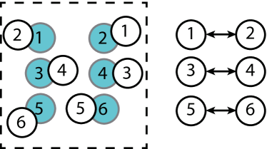
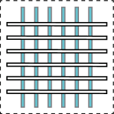
When there is no restriction on object geometry, MRB can easily reach the maximum possible $n-1$ for an $n$ object instance, even in the URBM case. An example of when this happens is given in Fig. 10, where $n=6$ thin cuboids are aligned horizontally in $\mathcal{A}_{1}$, one above the other. The cuboids are vertically aligned in $\mathcal{A}_{2}$. Every pair of start pose and goal pose then induce a (unique) dependency. Clearly, this yields a bidirectional $K_{6}$ labeled dependency graph in the LRBM case and a $K_{6,6}$ unlabeled dependency graph in the URBM case. For both, $n-1=5$ objects must be moved to buffers before the problem can be resolved. The example readily generalizes to an arbitrary number of objects.

Proposition 4.

MRB lower bound is $n-1$ for $n$ objects for both LRBM and URBM, which is the maximum possible, even for uniform convex objects.

Figure 10: An instance with 6 cuboids where horizontal and vertical sets represent start and goal poses, respectively. An arbitrary labeling of the objects may be given in the labeled setting.

The lower bound on MRB being $\Omega(n)$ is undesirable, but it seems to depend on having objects that are thin; everyday objects are not often like that. An ensuing question of high practical value is then: what happens when the footprint of the objects is “fat”? Next, we establish that, the lower bound drops to $\Omega(\sqrt{n})$ for uniform cylinders, which approximate many real-world objects/products. Furthermore, we show that this lower bound is tight for URBM (in Section 5.2).

For convenience, assume $n$ is a perfect square, i.e., $n=m^{2}$ for some integer $m$. To establish the $\Omega(\sqrt{n})$ lower bound, a grid-like unlabeled dependency graph is used, which we call a dependency grid, where $\mathcal{A}_{1}$ and $\mathcal{A}_{2}$ have similar patterns with $\mathcal{A}_{2}$ offset from $\mathcal{A}_{1}$ to the left (or right/above/below) by the length of one grid edge. An illustration of a portion of such a setup is given in Fig. 11. We use $\mathcal{D}(w,h)$ to denote a dependency grid with $w$ columns and $h$ rows.

Lemma 2.

Given a URBM instance with $n=m^{2}$ objects and whose dependency graph is $\mathcal{D}(m,2m)$, its MRB is lower bounded by $\Omega(m)=\Omega(\sqrt{n})$

Because the proof has limited relevance to the delivery of the main contributions of the paper, we highlight the main idea and refer the readers to the appendix for the complete proof. What we show is that, for certain unlabeled TORO instance with $n$ objects with such a dependency graph, at least $\Omega(\sqrt{n})$ objects must be moved to buffers simultaneous to solve the TORO instance.

Figure 11: A URBM instance (left) and its unlabeled dependency graph (right), a $4\times 3$ dependency grid. Unshaded (resp., shaded) discs/vertices indicate start poses (resp., goal poses).

Because URBM  instances always have lower or equal MRB than the LRBM  instances with the same objects and goal placements, the conclusion of Lemma 2 directly applies to LRBM. Therefore, we have

Theorem 3.

For both URBM and LRBM with $n$ uniform cylinders, MRB is lower bounded by $\Omega(\sqrt{n})$.

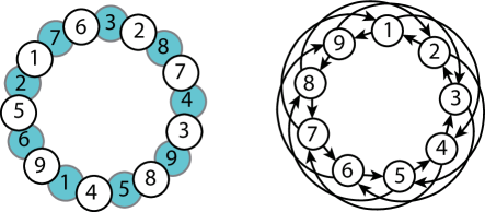
For uniform cylinders, while the lower bound on URBM is tight (as shown in Section 5.2), we do not know whether the lower bound on LRBM is tight; our conjecture is that $\Omega(\sqrt{n})$ is not a tight lower bound for LRBM. Indeed, the $\Omega(\sqrt{n})$ lower bound can be realized when uniform cylinders are simply arranged on a cycle, an illustration of which is given in Fig. 12. For a general construction, for each object $o_{i}$, let $o_{i}$ depend on $o_{(i-1\mod n)}$ and $o_{(i+\sqrt{n}\mod n)}$, where $n$ is the number of objects in the instance. From the labeled dependency graph, we can construct the actual LRBM instance where start and goal arrangements both form a cycle. It can be shown that when $n/2$ objects are at the goal poses, $\Omega(\sqrt{n})$ objects are at the buffer. We omit the proof, which is similar in spirit to that for Lemma 2.

Figure 12: An example of a 9-object LRBM yielding $\Omega(\sqrt{n})$ MRB (left) and the corresponding dependency graph (right).

5.2 Upper Bounds on MRB  for URBM

We now establish, regardless of how $n$ uniform cylinders are to be rearranged, the corresponding URBM instance admits a solution using $\textsc{MRB}=O(\sqrt{n})$. Lower and upper bounds on URBM agree; therefore, the $O(\sqrt{n})$ bound is tight.

To prove the upper bound, We propose an $O(n\log(n))$-time algorithm SepPlan for the setting based on a vertex separator of $G^{\,u}$. SepPlan computes a sequence of goal vertices to be removed from the dependency graph. Given a sequence of goal vertices to be removed, the running buffer size at each moment equals $\max(0,\|N(g,G^{\,u})\|-\|g\|)$, where $g$ is the set of removed goal vertices at this moment, and $N(g,G^{\,u})$ is the set of neighbors of $g$ in $G^{\,u}$. We prove that SepPlan can find a rearrangement plan with $O(\sqrt{n})$ running buffers.

Input : $G^{\,u}(V,E)$: unlabeled dependency graph

Output : $\pi$: goal sequence

1 $\pi,V,E\leftarrow$ RemovalTrivialGoals($G^{\,u}(V,E)$)

2 if $V$ is $\emptyset$ then  return $\pi$ ;

3 $A,B,C\leftarrow$ Separator($G^{\,u}(V,E)$)

4 $\pi\leftarrow\pi+g(C)$

5 $A^{\prime}\leftarrow A-N(g(C),G^{\,u}(V,E))$

6 $B^{\prime}\leftarrow$ $B$$-N(g(C),G^{\,u}(V,E))$

7 $\pi_{A^{\prime}}\leftarrow$ SepPlan ($G^{\,u}(A^{\prime},E(A^{\prime}))$)

8 $\pi_{B^{\prime}}\leftarrow$ SepPlan ($G^{\,u}(B^{\prime},E(B^{\prime}))$)

9 if  $\delta(A^{\prime})\geq\delta(B^{\prime})$ then  $\pi\leftarrow\pi+\pi_{A^{\prime}}+\pi_{B^{\prime}}$ ;

10 else  $\pi\leftarrow\pi+\pi_{B^{\prime}}+\pi_{A^{\prime}}$ ;

11 return $\pi$

Algorithm 1 SepPlan

The algorithm is presented in Algo. 1. SepPlan consumes a graph $G^{\,u}(V,E)$, which is a subgraph of $G^{\,u}$ induced by vertex set $V$. To start with, the isolated goal vertices or those with only one dependency in $G^{\,u}(V,E)$ can be removed without using buffers (Line 1). After that, $V$ can be partitioned into three disjointed subsets $A$, $B$ and $C$ [60] (Line 3), such that there is no edge connecting vertices in $A$ and $B$, $|A|,|B|\leq 2|V|/3$, and $|C|\leq 2\sqrt{2|V|}$ (Fig. 13(a)). For the start vertices in $C$ and the neighbors of the goal vertices in $C$, we remove them from $G^{\,u}$. Since there are at most $5$ neighbors for each goal vertex, there are at most $10\sqrt{2|V|}$ objects moved to the buffer in this operation. After that, we remove the goal vertices in $C$, which should be isolated now (Line 4). Function $g(\cdot)$ obtains the goal vertices in a given vertex set. Let $A^{\prime}$, $B^{\prime}$ be the remaining vertices in $A$ and $B$ (Line 5-6). And correspondingly, let $C^{\prime}$ be the removed vertices, i.e., $C^{\prime}:=(A\bigcup B\bigcup C)\backslash(A^{\prime}\bigcup B^{\prime})$. Function $N(\cdot,\cdot)$ obtains the neighbors of a vertex set in a given dependency subgraph. With the removal of $C^{\prime}$ from $G^{\,u}$, $A^{\prime}$ and $B^{\prime}$ form two independent subgraphs (Fig. 13(b)). We can deal with the subgraphs one after the other by recursively calling SepPlan (Fig. 13(c)) (Line 7-8). Let $\delta(V^{\prime}):=|g(V^{\prime})|-|s(V^{\prime})|$ where $g(V^{\prime})$ and $s(V^{\prime})$ are the goal and start vertices in a vertex set $V^{\prime}$ respectively. Between vertex subsets $A^{\prime}$ and $B^{\prime}$, we prioritize the one with larger $\delta(\cdot)$ value(Line 9-10). That is because, after solving a rearrangement subproblem induced by a vertex set $V^{\prime}$, there is $\delta(V^{\prime})$ fewer objects in buffers or $\delta(V^{\prime})$ more available goal poses.

\begin{overpic}[width=260.17464pt]{figures/separator-eps-converted-to.pdf} \put(12.0,-5.0){(a)} \put(46.0,-5.0){(b)} \put(82.0,-5.0){(c)} \end{overpic}

Figure 13: The recursive solver SepPlan for URBM. (a) A $O(\sqrt{|V|})$ vertex separator for the planar dependency graph. (b) By removing the start vertices in $C$ and the neighbors of the goal vertices in $C$, the remaining graph consists of two independent subgraphs and isolated goal poses in $C$. (c) The problem can be solved by recursively calling SepPlan.

As shown in detail in the appendix, SepPlan guarantees an MRB upper bound of $\dfrac{20}{1-\sqrt{2/3}}\sqrt{n}$.

Theorem 4.

For URBM with $n$ uniform cylinders, a polynomial time algorithm can compute a plan with $O(\sqrt{n})$ RB, which implies that MRB is bounded by $O(\sqrt{n})$.

6 Algorithms

In this section, several algorithms for computing solutions for TORO tasks under various MRB objectives are described. The hardness result (Theorem 2) suggests that the challenge in computing MRB solutions for TORO resides with filtering through an exponential number of vertex linear orderings of the dependency graph. This leads to our algorithms being largely search-based, which are enhanced with many effective heuristics.

We first describe a dynamic programming-based method for LRBM (Sec. 6.1). Then, we propose a priority queue-based method in Sec. 6.2 for URBM. Furthermore, a significantly faster depth-first modification of DP for computing MRB is provided in Sec. 6.3. Finally, we also developed an integer programming model, denoted $\textsc{TB}_{\textsc{MRB}}$, for computing the minimum total number of buffers needed subject to the MRB constraint, which is compared with the algorithm that computes the minimum total buffer without the MRB constraint, denoted as $\textsc{TB}_{\textsc{FVS}}$, from [1]. A brief description of $\textsc{TB}_{\textsc{MRB}}$ is given in Sec. 6.4.

6.1 Dynamic Programming (DP) for LRBM

As established in Sec. 4.2, a rearrangement plan in LRBM can be represented as a linear ordering of object labels. That is, given an ordering of objects, $\pi$, we start with $o_{\pi(1)}$. If $x^{g}_{\pi(1)}$ is not occupied, then $o_{\pi(1)}$ is directly moved there. Otherwise, it is moved to a buffer location. We then continue with the second object in the order, and so on. After we work with each object in the given order, we always check whether objects in buffers can be moved to their goals, and do so if an opportunity is present. We now describe a dynamic programming (DP) algorithm for computing such a linear ordering that yields the MRB.

The pseudo-code of the algorithm is given in Algo. 2. The algorithm maintains a search tree $T$, each node of which represents an arrangement where a set of objects $S$ have left the corresponding start poses. We record the objects currently at the buffer ($T[S]$.b) and the minimum running buffer from the start arrangement $\mathcal{A}_{1}$ to the current arrangement ($T[S].\textsc{MRB}$). The DP starts with an empty $T$. We let the root node represent $\mathcal{A}_{1}$ (Line 1). At this moment, there is no object in the buffer and the MRB is 0(Line 2-3). And then we enumerate all the arrangements with $|S|=$ 1, 2, $\cdots$ and finally $n$(Line 4-5). For arbitrary $S$, the objects at the buffer are the objects in $S$ whose goal poses are still occupied by other objects (Line 6), i.e., $\{o\in S|\exists o^{\prime}\in\mathcal{O}\backslash S,(o,o^{\prime})\in A\}$, where $A$ is the set of arcs in $G^{\,\ell}$. $T[S].\textsc{MRB}$, the minimum running buffer from the root node $T[\emptyset]$ to $T[S]$, depends on the last object $o_{i}$ added into $S$ and can be computed by enumerating $o_{i}$ (Line 7-20):

$$\begin{array}[]{l}T[S].\textsc{MRB}=\displaystyle\min_{o_{i}\in S}\max(T[S\backslash\{o_{i}\}].\textsc{MRB},\\ \qquad\qquad\qquad\qquad\qquad|T[S\backslash\{o_{i}\}].b|\ +\text{TC}(S\backslash\{o_{i}\},S)),\end{array}$$

where the transition cost TC is given as

$$\text{TC}(S\backslash\{o_{i}\},S)=\begin{cases}1,\ o_{i}\in T[S].b,\\ 0,\ otherwise,\end{cases}$$

with $x^{g}_{i}$ currently occupied (Line 10), the transition cost is due to objects dependent on $o_{i}$ cannot be moved out of the buffer before moving $o_{i}$ to the buffer (Line 11). Specifically, $T[S\backslash\{o_{i}\}].\textsc{MRB}$ is the previous MRB and $|T[S\backslash\{o_{i}\}].b|\ +\text{TC}(S\backslash\{o_{i}\},S)$ is the running buffer size in the new transition. If $T[S].\textsc{MRB}$ is minimized with $o_{i}$ being the last object in $S$ from the starts, then $T[S\backslash\{o_{i}\}]$ is the parent node of $T[S]$ in $T$ (Line 16-19). Once $T[\mathcal{O}]$ is added into $T$, $T[\mathcal{O}].\textsc{MRB}$ is the MRB of the instance (Line 23) and the path in $T$ from $T[\emptyset]$ to $T[\mathcal{O}]$ is the corresponding solution to the instance.

Input : $G^{\,\ell}(\mathcal{O},A)$: labeled dependency graph

Output : MRB: the minimum number of running buffers

1 $T.root\leftarrow\emptyset$

$T[\emptyset].b\leftarrow\emptyset$ % objects currently at the buffer

$T[\emptyset].\textsc{MRB}\leftarrow 0$ % current minimum running buffer

2 for $1\leq k\leq|\mathcal{O}|$ do

       % enumerate cases where $k$ objects have left the start poses

3       for $S\in\text{k-combinations of }\mathcal{O}$ do

4             $T[S].b\leftarrow\{o\in S\mid\exists o^{\prime}\in\mathcal{O}\backslash S,(o,o^{\prime})\in A\}$

             % Find the MRB from $T[\emptyset]$ to $T[S]$

5             $T[S].\textsc{MRB}\leftarrow\infty$

6             for $o_{i}\in S$ do

7                   $parent=S\backslash\{o_{i}\}$

8                   if $o_{i}\in T[S].b$ then

9                         $RB\leftarrow\max(T[parent].\textsc{MRB}$, $|T[parent].b|+1$)

10                   end if

11                  else

12                         $RB\leftarrow T[parent].\textsc{MRB}$

13                   end if

14                  if RB$<T[S].\textsc{MRB}$ then

15                         $T[S].\textsc{MRB}\leftarrow RB$

16                         $T[S].parent\leftarrow$ $parent$

17                   end if

18                  

19             end for

20            

21       end for

22      

23 end for

24 return $T[\mathcal{O}]$.MRB

Algorithm 2 Dynamic Programming for LRBM

For the LRBM instance in Fig. 3, Tab. 1 shows $T[S].\textsc{MRB}$ with different last-object options when $S=\{o_{2},o_{5},o_{6}\}$. If the last object $o_{i}$ is $o_{5}$, then we need to move $o_{5}$ into the buffer before moving $o_{6}$ out of the buffer. Therefore, even though the buffer size of the parent node and the current node are both 2, there is a moment when all of the three objects are at the buffer. However, when we choose $o_{2}$ or $o_{6}$ as the last object to add, the $T[S].\textsc{MRB}$ becomes 2.

Table 1: $T[S].\textsc{MRB}$ for different last objects ($[p]=[parent]$)

Last object	$T[p].\textsc{MRB}$	$T[p].b$	$T[S].b$	$T[S].\textsc{MRB}$
$o_{2}$	1	{$o_{5}$}	{$o_{2}$, $o_{5}$}	2
$o_{5}$	2	{$o_{2}$, $o_{6}$}	{$o_{2}$, $o_{5}$}	3
$o_{6}$	2	{$o_{2}$, $o_{5}$}	{$o_{2}$, $o_{5}$}	2

6.2 A Priority Queue-Based Method for URBM

Similar to LRBM, rearrangement plans for URBM can be represented by a linear ordering of goal vertices in $G^{\,u}$. We can compute the ordering that yields MRB by maintaining a search tree as we have done in Algo. 2. Each node $T[g]$ in the tree represents an arrangement where a set of goal vertices $g$ have been removed from $G^{\,u}$. The remaining dependencies of $T[g]$ is an induced graph of $G^{\,u}$, formed from $V(G^{\,u})\backslash(g\cup N(g,G^{\,u}))$ where $V(G^{\,u})$ is the vertex set of $G^{\,u}$, $N(g,G^{\,u})$ is the neighbors of $g$ in $G^{\,u}$. When the goal vertices $g$ are removed from $G^{\,u}$, the running buffer size is $max(0,|N(g)|-|g|)$, i.e., the number of objects cleared away minus the number of available goal poses. Specifically, when $|N(g)|>|g|$, some objects are in buffers; when $|N(g)|<|g|$, some goal poses are available; when $|N(g)|=|g|$, the cleared objects happen to fill all the available goal poses. Given an induced graph $I(g)$, denote the goal vertices with no more than one neighbor in $I(g)$ as free goals. We make two observations. First, given an induced graph $I(g)$, we can always prioritize the removal of free goals without optimality loss. Second, multiple free goals may appear after a goal vertex is removed. For example, in the instance shown in Fig. 3(a), when the vertex representing $x^{5}_{g}$ is removed, $x^{2}_{g}$, $x^{3}_{g}$, and $x^{4}_{g}$ become free goals and can be added to the linear ordering in an arbitrary order. Denote nodes without free goals in the induced graph as key nodes. In conclusion, the key nodes in the search tree may be sparse and enumerating all possible nodes with DP carries much overhead.

As such, instead of exploring the search tree layer by layer like DP, we maintain a sparse tree with a priority queue $Q$. While each node still represents an arrangement, each edge in the tree represents actions to clear out the next goal pose $x_{i}^{g}$. The corresponding child node of the edge represents the arrangement where $x_{i}^{g}$ and free goals are removed from the induced graph. Similar to A*, we always pop out the key node with the smallest MRB in $Q$. We denote this priority queue-based search method PQS.

6.3 Depth-First Dynamic Programming

Both LRBM and URBM can be viewed as solving a series of decision problems, i.e., asking whether we can find a rearrangement plan with $k=1,2,\ldots$ running buffers. As dynamic programming is applied to solve such decision problems, instead of performing the more standard breadth-first exploration of the search tree, we identified that a depth-first exploration is much more effective. We call this variation of dynamic programming DFDP, which is a fairly straightforward alteration of a standard DP procedure. The high-level structure of DFDP is described in Algo. 3. It consumes a dependency graph and returns the minimum running buffer size for the corresponding instance. Essentially, DFDP fixes the running buffer size RB and checks whether there is a plan requiring no more than RB running buffers. As the search tree (see Sec. 6.1) is explored, depth-first exploration is used instead of breadth-first (Line 4).

Input : $G^{\,\ell}$: labeled dependency graph

Output : RB: the minimum number of running buffers

1 RB$\leftarrow 0$

2 while not time exceeded do

3       $T$.root $\leftarrow\emptyset$

4       $T\leftarrow$ Depth-First-Search($T$,$\emptyset$, RB, $G^{\,\ell}$)

5       if  $\mathcal{O}\in T$ then return RB;

6       else RB+=1;

7      

8 end while

Algorithm 3 Dynamic Programming with Depth-First Exploration

The details of the depth-first exploration are shown in Algo. 4. Similar to DP, each node in the tree represents an object state indicating whether an object is at the start pose, the goal pose, or external buffers. And as described in Sec. 4.2, essential object states can be represented by the set of objects $S$ that have picked up from start poses. If $S$ is $\mathcal{O}$, then all the objects are at the goal poses and we find a path on the search tree from the start state to the goal state (Line 1). Given the set of objects away from the start poses $S$, we can get the sets of objects at start poses $S_{S}$, goal poses $S_{G}$, and external buffers $S_{B}$ (Line 2). Specifically, $S_{S}=\mathcal{O}\backslash S$, $S_{G}$ are the objects in $S$ that have no dependency in $S_{S}$, and $S_{B}$ are the objects in $S$ that have dependencies in $S_{S}$. We further explore child nodes of the current state by moving one object away from the start pose (Line 3). By checking the dependencies in $G^{\,\ell}(\mathcal{O},A)$, we determine whether this object should be moved to buffers or its goal pose (Line 4). The transition from $S$ to $S\bigsqcup\{o\}$ fails if the external buffers are overloaded or the child node has been explored (Line 5). Otherwise, we can add $S\bigsqcup\{o\}$ into the tree (Line 7) and explore the new node (Line 8). The algorithm returns a tree.

Input :  $T$: Search Tree; $S$: The set of objects away from start poses; $RB$: Running buffer size; $G^{\,\ell}(\mathcal{O},A)$: labeled dependency graph

Output : $T$

1 if $S$ is $\mathcal{O}$ then return $T$;

2 $S_{S}$, $S_{G}$, $S_{B}$ = GetState($S$)

3 for $o\in S_{S}$ do

4       $ToBuffer$=CollisionCheck($S_{S}\backslash\{o\}$,$o$, $G^{\,\ell}$)

5       if (ToBuffer and $\|S_{B}\|+1>$RB) or ($S\bigsqcup\{o\}\in T$) then return $T$;

6       else

7             AddNode($T$, $S$, $S\bigsqcup\{o\}$)

8             $T$ $\leftarrow$ Depth-First-Search($T$, $S\bigsqcup\{o\}$, RB, $G^{\,\ell}$)

9             if  $\mathcal{O}\in T$ then return $T$;

10            

11       end if

12      

13 end for

return $T$

Algorithm 4 Depth-First-Search

The intuition is that, when there are many rearrangement plans on the search tree that do not use more than $k$ running buffers, a depth-first search will quickly find such a solution, whereas a standard DP must grow the full search tree before returning a feasible solution. A similar depth-first exploration heuristic is used in [72].

6.4 Minimizing Total Buffers Subject to MRB Constraints

We also construct a Mixed Integer Programming(MIP) model minimizing MRB or total buffers. Let binary variables $c_{i,j}$ represent the dependency graph $G^{\,\ell}$: $c_{i,j}=1$ if and only if $(i,j)$ is in the arc set of $G^{\,\ell}$. Let $y_{i,j}(1\leq i<j\leq n)$ be the binary sequential variables: $y_{i,j}=1$ if and only if $o_{i}$ moves out of the start pose before $o_{j}$. $y_{i,j}$ are used to represent the ordering of actions. We further introduce two sets of binary variables $g_{i,j}$ and $b_{i,j}(1\leq i,j\leq n)$ to indicate object positions at each moment. $g_{i,j}=1$ indicates that $o_{j}$ has no dependency on other objects when moving $o_{i}$ from the start pose. In other words, the goal pose of $o_{j}$ is available at the moment. $b_{i,j}=1$ indicates that $o_{j}$ stays at the buffer after moving $o_{i}$ away from the start pose. Finally, binary variables $B_{i}=1$ if and only if $o_{i}$ is moved to a buffer at some point. The objective function consists of two terms: the total buffer term and running buffer term. The total buffer term, scaled by $\alpha$, counts the number of objects that need buffer locations. MRB is represented with an integer variable $K$ and scaled by $\beta$. To minimize total buffers subject to MRB constraints, we set $\alpha=1,\beta=n$. The objective function is adaptable to different demands on rearrangement plans. Specifically, when $\alpha=0$,$\beta>0$, the MIP model minimizes MRB. When $\alpha>0$, $\beta=0$, the MIP model minimizes total buffers, i.e. total actions in the rearrangement plan. When $\alpha/\beta>n-1$, the MIP model first minimizes total buffers, and then minimizes running buffers. When $\beta/\alpha>n-1$, the MIP model first minimizes running buffers, and then minimizes total buffers.

In the MIP model, Constraints 2 imply the rules for sequential variables to make sure a valid ordering of indices $1,\dots,n$ can be encoded from $y_{i,j}$. Constraints 3 imply that $B_{j}=1$ if $o_{j}$ has been to buffers in the plan. Constraints 4 imply that MRB $K$ is lower bounded by the maximum number of objects concurrently placed in buffers. With Constraints 5 and 6, $g_{i,j}=0$ if and only if $o_{j}$ depends on an object $o_{k}$ which is still at the start pose when $o_{i}$ is moved. With Constraints 7-9, $b_{i,j}=1$ if and only if $o_{j}$ is moved before $o_{i}$ and the goal pose is still unavailable when $o_{i}$ is moved from the start pose.

$$\arg\min\alpha[\sum_{i=1}^{n}B_{i}]+\beta K$$ (1)

$$0\leq y_{i,j}+y_{j,k}-y_{i,k}\leq 1\ \ \ \forall 1\leq i<j<k\leq n$$ (2)

$$B_{j}\geq\sum_{1\leq i\leq n}\dfrac{b_{i,j}}{n}\ \ \ \forall 1\leq j\leq n$$ (3)

$$K\geq\sum_{1\leq j\leq n}b_{i,j}\ \ \ \forall 1\leq i\leq n$$ (4)

$$\begin{split}\sum_{1\leq k<i}\dfrac{c_{j,k}(1-y_{k,i})}{n}+\sum_{i<k\leq n}\dfrac{c_{j,k}y_{i,k}}{n}\leq 1-g_{i,j}\\ \forall 1\leq i,j\leq n\end{split}$$ (5)

$$\begin{split}1-g_{i,j}\leq\sum_{1\leq k<i}c_{j,k}(1-y_{k,i})+\sum_{i<k\leq n}c_{j,k}y_{i,k}\\ \forall 1\leq i,j\leq n\end{split}$$ (6)

$$\begin{split}\dfrac{g_{i,j}+y_{i,j}}{2}\leq 1-b_{i,j}\leq g_{i,j}+y_{i,j}\\ \forall 1\leq i<j\leq n\end{split}$$ (7)

$$\begin{split}\dfrac{g_{j,i}+(1-y_{i,j})}{2}\leq 1-b_{j,i}\leq g_{j,i}+(1-y_{i,j})\\ \forall 1\leq i<j\leq n\end{split}$$ (8)

$$b_{i,i}=1-g_{i,i}$$ (9)

7 Applications to In-Place Rearrangement with Bounded Workspace

Both LRBM and URBM allow external open space for temporary object displacements, computing rearrangement plans for TORO with external buffers (TORE). However, there are many practical rearrangement scenarios where objects have to be displaced inside the workspace. In this section, we apply the proposed algorithms to TORO with internal buffers (TORI). TORI seeks a feasible rearrangement plan minimizing the number of total actions. While solving TORE only deals with inherent constraints defined by the start and goal poses, some objects in TORI may be temporarily displaced inside the workspace and induce further acquired constraints. For instance, to solve the problem in Fig. 1 with external buffers, we can move the Pepsi can to an external buffer to break the cycle, move the Coke first and then Fanta to their goal locations, and finally, bring back the Pepsi can into the workspace. In TORI, we must find a temporary location for the Pepsi can in $\mathcal{W}$. If the buffer location overlaps with the goal of the Coke can (or the Fanta can), then the coke can (or the Fanta can) depends on the Pepsi can again. To avoid these acquired constraints, the buffer location needs to avoid the goals of Coke and Fanta. Due to acquired constraints arising from internal buffer selection, TORI, the problem we study in this section, is more challenging than TORE. Intuitively, selecting buffers inside the workspace (TORI) is much more difficult and constrained than using buffers outside the workspace (TORE) to store displaced objects. Since TORE has been shown to be computationally intractable [1], and is equivalent to a special case of TORI where the workspace is large enough that collision-free buffer locations are guaranteed, TORI is also NP-hard. Additionally, in TORI, it may be challenging to allocate valid buffer locations so it is necessary to limit the running buffer size. With this observation, we compute TORI solutions based on methods for LRBM and URBM.

In this section, We propose Tabletop Rearrangement with Lazy Buffers (TRLB), an effective framework for solving TORI based on algorithms mentioned in Sec. 6. We first describe a rearrangement solver with lazy buffer allocation (Sec. 7.1), where buffer allocation is delayed after DFDP computes a “rough” schedule of object movements. Finally, a preprocessing routine based on DFDP for URBM helps with further speedups (Sec. 7.2). To enhance scalability to larger and more cluttered instances, the TRLB framework (Sec. 7.3) recovers from buffer allocation failures.

7.1 Lazy Buffer Allocation

When an object stays at a buffer, it should avoid blocking the upcoming manipulation actions of other objects. Otherwise, either the object in the buffer or the manipulating object has to yield, which increases the number of necessary actions. In other words, we need to carefully choose acquired constraints. If we know the schedule of other objects in advance, a buffer can be selected to minimize unnecessary obstructions. This observation motivates solving the rearrangement problem in two steps: First, compute a primitive plan, which is an incomplete schedule ignoring acquired constraints; second, given the incomplete schedule as a reference, generate buffers to optimize the selection of acquired constraints.

7.1.1 Primitive Plan

To compute a primitive plan, we assume enough free space is available so that no acquired constraints will be created. This transforms the problem into a TORE problem, where each object is displaced at most once before it moves to the goal pose. Then, an object $o_{i}\in\mathcal{O}$ can have three primitive actions:

1. $(o_{i},s\rightarrow g)$: moving from $x^{s}_{i}$ to $x^{g}_{i}$;

2. $(o_{i},s\rightarrow b)$: moving from $x^{s}_{i}$ to a buffer;

3. $(o_{i},b\rightarrow g)$: moving from a buffer to $x^{g}_{i}$.

A primitive plan is a sequence of primitive actions; computing such a plan is similar to finding a linear vertex ordering [66, 65] of the dependency graph. Since we need to allocate buffer locations inside the workspace in the next phase of the algorithm, it is beneficial to limit the number of buffer positions that need to be concurrently allocated. We use DFDP to achieve this, which minimizes the number of running buffers.

7.1.2 Buffer Allocation

Free space inside the workspace $\mathcal{W}$ is scarce in cluttered spaces (e.g., Fig. 17) and acquired constraints must be dealt with through the careful allocation of buffers inside $\mathcal{W}$. We apply a greedy strategy to find feasible buffers based on a primitive plan (Algo. 5). The general idea is to incrementally add constraints on the buffers until we find feasible buffers for the whole primitive plan or terminate at a step where there are no feasible buffers for the primitive plan. In Algo. 5, $\mathcal{O}_{s},\mathcal{O}_{g}$, and $\mathcal{O}_{b}$ are the sets of objects currently at start poses, goal poses and buffers respectively.

Input : $\pi$: a primitive plan; $\mathcal{A}_{1}=\{x^{s}_{1},...,x^{s}_{n}\}$: start arrangement; $\mathcal{A}_{2}=\{x^{g}_{1},...,x^{g}_{n}\}$: goal arrangement

Output : $B$: buffers; TerminatingStep: the action step where buffer generation fails, $\infty$ if Success.

1 $\mathcal{O}_{s}$ $\leftarrow$ $\mathcal{O}$; $\mathcal{O}_{g}$, $\mathcal{O}_{b}$ $\leftarrow$ $\emptyset$; $B\leftarrow$ RandomPoses($\mathcal{O}$)

2 Constraints $\leftarrow$ InitializeConstraints();

3 for  $(o_{i},m)\in\pi$ do

4       if $m$ is s $\rightarrow$ b then

5             $\mathcal{O}_{b}$.add($o_{i}$)

6             Constraints[$o_{i}$]$\leftarrow$GetPoses($\mathcal{O}_{s}\bigcup\mathcal{O}_{g}-\{o_{i}\}$)

7            

8       end if

9      else if $m$ is b $\rightarrow$ g then

10             for $o\in\mathcal{O}_{b}\backslash\{o_{i}\}$ do  Constraints[$o$].add( $x^{g}_{i}$;

11            )

12       end if

13      

14 end for

15else

16       for $o\in\mathcal{O}_{b}$ do  Constraints[$o$].add( $x^{g}_{i}$;

17      )

18 end if

19Success, $B^{\prime}$ $\leftarrow$ BufferGeneration($\mathcal{O}_{b}$, Constraints, $B$)

20 if Success then

21       $B$ $\leftarrow$ $B^{\prime}$

22       $\mathcal{O}_{s},\mathcal{O}_{g},\mathcal{O}_{b}\leftarrow$ UpdateState($\mathcal{O}_{s},\mathcal{O}_{g},\mathcal{O}_{b}$)

23      

24 end if

25else  return $B$, $\pi$.index(action) ;

26

27 return $B$, $\infty$

Algorithm 5 Buffer Allocation

We start with $\mathcal{A}_{1}$ where all the objects are at start poses and the buffers are initialized at random poses (Line 1). We then initialize a mapping from $\mathcal{O}$ to the power set of object poses, indicating the set of obstacles to avoid when allocating buffer poses for the object (Line 2). Each action in $\pi$ indicates an object $o_{i}$ that is manipulated and the action $m$ performed (Line 3). If $o_{i}$ is moved to a buffer (Line 4), then we add it into $\mathcal{O}_{b}$ (Line 5). The current poses of other objects in $O_{s}\bigcup O_{g}$ are seen as fixed obstacles for $o_{i}$ (Line 6). If $o_{i}$ is leaving the buffer (Line 8), then other objects in $\mathcal{O}_{b}$ should avoid the goal pose $x^{g}_{i}$ of $o_{i}$ (Line 9). If $o_{i}$ is moving directly from $x^{s}_{i}$ to $x^{g}_{i}$ (Line 11, the “else” corresponds to $m$ being $s\to g$, i.e., directly go from start to goal), then all buffers for objects in the current $\mathcal{O}_{b}$ need to avoid $x^{g}_{i}$ (Line 12). After setting up acquired constraints, we generate new buffers for objects in $O_{b}$ to satisfy these constraints by either sampling or solving an optimization problem (Line 14). Old buffers in $B$ satisfying new constraints will be directly adopted. If feasible buffers are found (Line 15), then buffers and object states will be updated (Line 16-17). Otherwise, we return the feasible buffers computed and record the terminating step of the algorithm (Line 19). In the case of a failure, the returned buffers provide a partial plan.

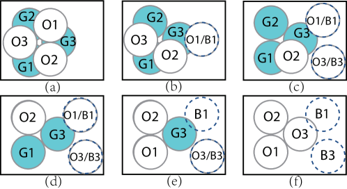
Fig. 14 illustrates the buffer allocation process via an example. The unshaded discs and shaded discs with solid line boundaries represent the current poses and goal poses respectively. The discs with dashed line boundaries represent the allocated buffers. When we move $o_{1}$ to a buffer $B_{1}$ (Fig. 14(b)), it only needs to avoid collision with $x^{s}_{2}$ and $x^{s}_{3}$. But as we move $o_{3}$ to a buffer, $B_{1}$ needs to avoid $o_{3}$’s buffer $B_{3}$ as well. To satisfy the added constraint, $B_{1}$ will be reallocated. Since the new buffers $B_{1}$ and $B_{3}$ (Fig. 14(c)) satisfy the constraints added in the following steps, they need not to be relocated. Note that the buffer originally selected for $o_{1}$ but then replaced will not appear in the resulting plan, i.e., $o_{1}$ will move directly to the new buffer (Fig. 14(c)-(f)). Algo. 5 works with one strongly connected component of the dependency graph at a time, treating objects in other components as fixed obstacles.

Once the feasible buffers are found, all the primitive actions can be transformed into feasible pick-n-place actions inside the workspace. And therefore, the primitive plan can be transformed into a rearrangement plan moving objects from $\mathcal{A}_{1}$ to $\mathcal{A}_{2}$. The function BufferGeneration is implemented by either sampling or solving an optimization problem, both of which are discussed below.

Figure 14: A working example with three objects defined in (a). The primitive plan is [($o_{1}$, s $\rightarrow$ b), ($o_{3}$, s $\rightarrow$ b), ($o_{2}$, s $\rightarrow$ g), ($o_{1}$, b $\rightarrow$ g), ($o_{3}$, b $\rightarrow$ g)]. Figures (b)-(f) show the steps of Alg. 5 after each action. The unshaded discs with dashed line boundaries ($B_{i}$) represent the buffers satisfying constraints up to each step. For each object $o_{i}$, the unshaded discs with solid line boundaries ($O_{i}$) represent the current poses and the shaded ($G_{i}$) discs represent goal poses.

Sampling

Given the object poses that buffers need to avoid so far, feasible buffers can be generated by sampling poses inside the free space. When objects stay in buffers at the same time, we sample buffers one by one and previously sampled buffers will be seen as obstacles for the latter ones.

Optimization

For cylindrical objects $o_{i}$ at $(x_{i},y_{i})$ with radius $r_{i}$, and $o_{j}$ at $(x_{j},y_{j})$ with radius $r_{j}$, they are collision-free when $(x_{i}-x_{j})^{2}+(y_{i}-y_{j})^{2}\geq(r_{i}+r_{j})^{2}$ holds. By further restricting the range of buffer centroids to assure they are in the workspace, the buffer allocation problem can be transformed into a quadratic optimization problem. For objects with general shapes, collision avoidance cannot be presented by inequalities of object centroids. We can construct the optimization problem with $\phi$ functions of the objects [73] and solve the problem with gradients.

7.2 Preprocessing

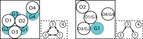
In dense environments, allocating buffers is hard, motivating minimizing the number of running buffers, which is generally low even in high-density settings in URBM. Based on this, for each component of the dependency graph that is not isolated vertex or simple cycle, we first solve it as if it is an unlabeled instance. After this preprocessing step, all the components in the resulting labeled instance are either simple cycles ($\textsc{MRB}=1$) or isolated vertices($\textsc{MRB}=0$). Fig. 15 shows an example of preprocessing. $o_{1}$, $o_{2}$, and $o_{3}$ form a complete graph, where at least two objects need to be placed at buffers simultaneously. We conduct preprocessing of the three-vertex component by moving $o_{2}$ to a buffer position, $o_{1}$ to $x^{g}_{3}$ and $o_{3}$ to $x^{g}_{2}$. $o_{2}$ will not move to $x^{g}_{1}$ since it does not occupy other goal poses. The preprocessing step needs one buffer and the resulting rearrangement problem is monotone.

Figure 15: A four-object example of preprocessing. The unshaded and shaded discs represent current and goal arrangements respectively. Before preprocessing (left), two buffers need to be allocated synchronously. After preprocessing (right), the problem becomes monotone.

7.3 Solving TORI with Lazy Buffers (TRLB)

The TRLB framework builds on the insight that a new TORI instance is generated when lazy buffer allocation fails. The new instance has the same goal $\mathcal{A}_{2}$ as the original one but some progress has been made in solving the TORI task. There are two straightforward implementations of TRLB: forward search and bidirectional search. In the first case, by accepting partial solutions, a rearrangement plan can be computed by developing a search tree $T$ rooted at $\mathcal{A}_{1}$. In the search tree $T$, nodes are feasible arrangements and edges are partial plans containing a sequence of collision-free actions. When buffer allocation fails, we add the resulting arrangement into the tree and resume the rearrangement task from a random node in $T$. This randomness and the randomness in primitive plan computation and buffer allocation allows TRLB to recover from failures.

Input :  $\mathcal{A}_{1}$, $\mathcal{A}_{2}$, $max\_time$

Output :  Search trees: $T_{1}$, $T_{2}$

1 $T_{1}$.root, $T_{2}$.root$\leftarrow$ $\mathcal{A}_{1}$, $\mathcal{A}_{2}$

2 while not exceeding $max\_time$ do

3       $\mathcal{A}_{rand}\leftarrow$ RandomNode($T_{1}$)

4       $\mathcal{A}_{new1}\leftarrow$ LazyBufferAllocation($\mathcal{A}_{rand}$, $T_{2}$.root)

5       $T_{1}$.add($\mathcal{A}_{new1}$)

6       if $\mathcal{A}_{new1}$ is $T_{2}$.root then return $T_{1}$, $T_{2}$;

7       $\mathcal{A}_{near}\leftarrow$ NearestNode($\mathcal{A}_{new1}$, $T_{2}$)

8       $\mathcal{A}_{new2}\leftarrow$ LazyBufferAllocation($\mathcal{A}_{near}$, $\mathcal{A}_{new1}$)

9       $T_{2}$.add($\mathcal{A}_{new2}$)

10       if $\mathcal{A}_{new2}$ is $\mathcal{A}_{new1}$ then return $T_{1}$, $T_{2}$;

11       $T_{1},T_{2}\leftarrow T_{2},T_{1}$

12      

13 end while

Algorithm 6 TRLB with Bidirectional Search

In bidirectional search, two search trees rooted at $\mathcal{A}_{1}$ and $\mathcal{A}_{2}$ are developed. This more involved procedure is shown in Algo. 6, which computes two search trees that connect $\mathcal{A}_{1}$ and $\mathcal{A}_{2}$. In Line 1, the trees are initialized. For each iteration, we first rearrange between a random node $\mathcal{A}_{rand}$ on $T_{1}$ to the root node of $T_{2}$ (Line 3-5). The function LazyBufferAllocation refers to the overall algorithm developed in Sec. 7.1. A found path yields a feasible plan for TORI (Line 6). Otherwise, we rearrange between the new arrangement $\mathcal{A}_{new1}$ and its nearest neighbor in $T_{2}$ (Line 7-9). If a path is found, then we find a feasible rearrangement plan for TORI (Line 10). Otherwise, we switch the trees and attempt rearrangement from the opposite side (Line 11).

8 Performance Evaluation of Simulations

Our evaluation focuses on uniform cylinders, given their prevalence in practical applications. For simulation studies, instances with different object densities are created, as measured by density level $\rho:=n\pi r^{2}/(h*w)$, where $n$ is the number of objects and $r$ is the base radius. $h$ and $w$ are the height and width of the workspace. In other words, $\rho$ is the proportion of the tabletop surface occupied by objects.

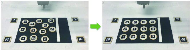
The evaluation is conducted on both random object placements and manually constructed difficult setups (e.g., dependency grids with $MRB=\Omega(\sqrt{n}$)). For generating test cases with high $\rho$ value, we invented a physic engine (we used Gazebo [74]) based approach for doing so. Within a rectangular box, we sample placements of cylinders at lower density and then also sample locations for some smaller “filler” objects (see Fig. 16, left). From here, one side of the box is pushed to reach a high density setting (Fig. 16, right), which is very difficult to generate via random sampling. By controlling the ratio of the two types of objects, different density levels can be readily obtained. Fig. 17 shows three random object placements for $\rho=0.2,0.4$ and $0.6$.

Figure 16: Generating dense instances using a physics-engine based simulator through compression of the left scene to the right scene.

Figure 17: Unlabeled arrangements with $\rho=0.2,0.4,0.6$ respectively.

From two randomly generated object placements with the same $\rho$ and $n$ values, a URBM instance can be readily created by superimposing one over the other. LRBM instances can be generated from URBM instances by assigning each object a random label in $[n]$ for both start and goal configurations.

For tabletop object rearrangement with external buffers (TORE), evaluated methods in different scenarios(labeled or unlabeled) are presented in Tab. 2. For tabletop object rearrangement with internal buffers (TORI), we present experiments comparing lazy buffer generation algorithms given different options(Tab. 3), including: (1) Primitive plan computation: running buffer minimization with DFDP (RBM), total buffer minimization with DP (TBM), random order (RO); (2) Buffer allocation methods: optimization (OPT), sampling (SP); (3) High-level planners: one-shot (OS), forward search tree (ST), bidirectional search tree (BST); and (4) With or without preprocessing (PP). Here, the one-shot (OS) planner is using primitive plans and buffer allocation (Sec. 7.1) without tree search (Sec. 7.3). In OS, we attempt to compute a feasible rearrangement plan up to $30|\mathcal{O}|$ times before announcing a failure. A full TRLB algorithm is a combination of components, e.g., RBM-SP-BST stands for using the primitive plans that minimize running buffer size, performing buffer allocation by sampling, maintaining a bidirectional search tree, and doing so without preprocessing.

To highlight the application of RBM in TORI, we only compare methods in primitive plan computation and evaluate the effect of our preprocessing routine. A complete ablation study is presented in [3].

Table 2: Evaluated methods for TORE.

Problems	Methods
LRBM	DFDP, DP, $\textsc{TB}_{\textsc{FVS}}$, $\textsc{TB}_{\textsc{MRB}}$
URBM	DFDP, PQS

Table 3: Evaluated methods for TORI.

Components	Methods
Primitive plan computation	RBM, TBM, RO
Buffer allocation methods	OPT, SP
High level planners	OS, ST, BST
Preprocessing	PP

The proposed algorithms are implemented in Python and all experiments are executed on an Intel^® Xeon^® CPU at 3.00GHz. For solving MIP, Gurobi 9.16.0 [75] is used.

8.1 LRBM over Random Instances

In Fig. 18, we compare the effectiveness of DP and DFDP, in terms of computation time and success rate, for different densities. Each data point is the average of $30$ test cases minus the unfinished ones, if any, subject to a time limit of $300$ seconds per test case. For LRBM, we are able to push to $\rho=0.4$, which is fairly dense. The results clearly demonstrate that DFDP significantly outperforms the baseline DP. Based on the evaluation, both methods can be used to tackle practical-sized problems (e.g., tens of objects), with DFDP demonstrating superior efficiency and robustness.

\begin{overpic}[width=260.17464pt]{figures/Time-eps-converted-to.pdf} \put(0.5,-22.5){ \includegraphics[width=260.17464pt]{figures/Rate-eps-converted-to.pdf}} \end{overpic}

Figure 18: Performance of DFDP and DP over LRBM. The top row shows the average computation time (s) and the bottom row the success rate, for density levels $\rho=0.2,0.3$, $0.4$, from left to right. The $x$-axis denotes the number of objects involved in a test case.

The actual MRB sizes for the same test cases from Fig. 18 are shown in Fig. 19 on the left. We observe that MRB is rarely very large even for fairly large LRBM instances. The size of MRB appears correlated to the size of the largest connected component of the underlying dependency graph, shown in Fig. 19 on the right.

\begin{overpic}[width=143.09538pt]{figures/MRB_Tendency-eps-converted-to.pdf} \end{overpic}

\begin{overpic}[width=143.09538pt]{figures/SCC_Tendency-eps-converted-to.pdf} \end{overpic}

Figure 19: For LRBM instances with $\rho=0.2$-$0.4$ and $n=20$-$100$, the left figure shows average MRB size and range. The right figure shows the size of the largest connected component of the dependency graph.

For LRBM with $\rho=0.3$ and $n$ up to $50$, we computed the MFVS sizes using $\textsc{TB}_{\textsc{FVS}}$ (which does not scale to higher $\rho$ and $n$) and compared that with the MRB sizes, as shown in Fig. 20 (a). We observe that the MFVS is about twice as large as MRB, suggesting that MRB provides more reliable information for estimating the design parameters of pick-n-place systems. For these instances, we also computed the total number of buffers needed subject to the MRB constraint using $\textsc{TB}_{\textsc{MRB}}$. Out of about $150$ instances, only $1$ showed a difference as compared with MFVS (therefore, this information is not shown in the figure). In Fig. 20 (b), we provided computation time comparison between $\textsc{TB}_{\textsc{FVS}}$ and $\textsc{TB}_{\textsc{MRB}}$, showing that $\textsc{TB}_{\textsc{MRB}}$ is practical, if it is desirable to minimize the total buffers after guaranteeing the minimum number of running buffers.

\begin{overpic}[width=229.81805pt]{figures/IP_FVS_Comparison-eps-converted-to.pdf} \put(22.0,-3.5){{\small(a)}} \put(76.0,-3.5){{\small(b)}} \end{overpic}

Figure 20: (a) Comparison between size of MRB and MFVS. (b) Computation time comparison between $\textsc{TB}_{\textsc{FVS}}$ and $\textsc{TB}_{\textsc{MRB}}$.

Considering our theoretical findings and the evaluation results, an important conclusion can be drawn here is that MRB is effectively a small constant for random instances, even when the instances are very large. Also, minimizing the total number of buffers used subject to MRB constraint can be done quickly for practical-sized problems.

8.2 URBM over Random Instances

For URBM, we carry out a similar performance evaluation as we have done for LRBM. Here, PQS and DFDP are compared. For each combination of $\rho$ and $n$, $100$ random test cases are evaluated. Notably, we can reach $\rho=0.6$ with relative ease. From Fig. 21, we observe that DFDP is more efficient than PQS, especially for large-scale dense settings. In terms of the MRB size, all instances tested have an average MRB size between $0$ and $0.7$, which is fairly small (Fig. 22). Interestingly, we witness a decrease of MRB as the number of objects increases, which could be due to the lessening “border effect” of the larger instances. That is, for instances with fewer objects, the bounding square puts more restriction on the placement of the objects inside. For larger instances, such restricting effects become smaller. We mention that the total number of buffers for random URBM cases subject to MRB constraints are generally very small.

\begin{overpic}[width=260.17464pt]{figures/Unlabeled_Time-eps-converted-to.pdf} \put(0.5,-22.5){ \includegraphics[width=260.17464pt]{figures/Unlabeled_Rate-eps-converted-to.pdf}} \end{overpic}

Figure 21: Performance of DFDP and PQS over URBM. The top row shows the average computation time and the bottom row shows the success rate, for density levels $\rho=0.4,0.5,0.6$, from left to right.

Figure 22: Average MRB size for URBM instances with $\rho=0.4-0.6$ and $n=20-100$. For $\rho=0.4$ and $0.5$, the MRB sizes are near zero as the number of objects goes beyond $20$.

8.3 Manually Constructed Difficult Cases of TORE

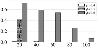
In the random scenario, the running buffer size is limited. In particular, for LRBM, the dependency graph tends to consist of multiple strongly connected components that can be dealt with independently. We further show the performance of DFDP on the instances with $\textsc{MRB}=\Theta(\sqrt{n})$. We evaluate three kinds of instances: (1) UG: $m^{2}$-object URBM instances whose $G^{\,u}$ are dependency grid $\mathcal{D}(m,2m)$ (e.g., Fig. 11); (2) LG: $m^{2}$-object LRBM instances whose start and goal arrangements are the same as the instances in (1). (3) LC: $m^{2}$-object LRBM instances with objects placed on a cycle (Fig. 12). The computation time and the corresponding MRB are shown in Fig. 23. For LG instances, the labels are randomly assigned. We try 30 test cases and then plot out the average. We observe that the MRB is much larger for these handcrafted instances as compared with random instances with similar density and number of objects.

\begin{overpic}[width=260.17464pt]{figures/Special_Case-eps-converted-to.pdf} \end{overpic}

Figure 23: For handcrafted cases and different numbers of objects, the left figure shows the computation time by DFDP and the right figure the resulting MRB size.

8.4 Evaluation on TORI Instances

8.4.1 Ablation Study for Cylindrical Objects.

For evaluation, we present experiments with cylindrical objects to compare lazy buffer generation algorithms. A more detailed version of the ablation study is presented in [3]. We first compare the primitive plan computation options, using sampling-based buffer allocation (SP) and bidirectional tree search (BST). The results are shown in Fig. 24. Even though plans generated by TBM-SP-BST are slightly shorter than RBM-SP-BST, TBM is less scalable as either the density level or the number of objects in the workspace increases. Compared to RBM plans, individual RO plans can be generated almost instantaneously but we don’t see much benefit in computation time for the overall algorithm. The results indicate that minimizing MRB in primitive plan computation is beneficial as it results in efficient and high-quality TORI solutions.

\begin{overpic}[width=260.17464pt]{figures/primitive_03-eps-converted-to.pdf} \put(-1.5,-22.5){ \includegraphics[width=260.17464pt]{figures/primitive_05-eps-converted-to.pdf}} \end{overpic}

Figure 24: Comparison of primitive planners with $10$-$40$ cylinders and density levels $\rho=0.3$ (top), 0.5 (bottom) (left: computation time in seconds; middle: success rate; right: number of actions as multiples of $|\mathcal{O}|$).

We also integrate the  urbm-based preprocessing routine into the bi-directional search tree framework (RBM-SP-BST-PP) and compare it with RBM-SP-BST. The results (Fig. 25) suggest that preprocessing is effective in increasing the success rate in dense environments. In addition, preprocessing significantly speeds up computation in large-scale dense cases at the price of extra actions to execute preprocessing. By simplifying the dependency graph with preprocessing, less time is needed to compute a primitive plan.

\begin{overpic}[width=260.17464pt]{figures/PP_03-eps-converted-to.pdf} \put(-1.5,-22.5){ \includegraphics[width=260.17464pt]{figures/PP_05-eps-converted-to.pdf}} \end{overpic}

Figure 25: Comparison between lazy buffer allocation algorithms with and without preprocessing. There are 10-40 cylinders in the workspace at density levels $\rho=0.3$ (top), $0.5$ (bottom) (left: computation time in seconds; middle: success rate; right: number of actions as multiples of $|\mathcal{O}|$).

8.4.2 Comparison with Alternatives for Cylindrical Objects.

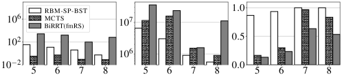
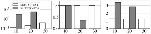
We compare the proposed method RBM-SP-BST with BiRRT(fmRS) [49] and an MCTS planner [76], which, to the best of our knowledge, are state-of-the-art planners for TORI. The MCTS planner is a C++ solver, while the other two methods are implemented in Python. Besides success rate, solution quality, and computation time, we also compare the number of collision checks which are time-consuming in most planning tasks. In Fig. 26, we compare the methods in large-scale problems with $\rho=0.3$. The success rate is $100\%$ for all. Our method, RBM-SP-BST, avoids repeated collision checks due to the use of the dependency graph. BiRRT(fmRS), which only uses dependency graphs locally, spends a lot of time and conducts a lot of collision checks to generate random arrangements. MCTS generates solutions with similar optimality but does so also with a lot of collision checking, which slows down the computation. We note that a value of $1$ in the right figure (number of actions) is the minimum possible, so both RBM-SP-BST and MCTS compute high-quality solutions, while RBM-SP-BST does slightly better. To sum up, in sparse large-scale instances, RBM-SP-BST is two magnitudes faster and conducts much fewer collision checks than the alternatives.

\begin{overpic}[width=260.17464pt]{figures/large_scale-eps-converted-to.pdf} \end{overpic}

Figure 26: Comparison of algorithms with 20-100 cylinders at density level $\rho=0.3$ (left: computation time in seconds; middle: number of collision checks; right: number of actions as multiples of $|\mathcal{O}|$).

Next, in Fig. 27, we compare the methods in “dense-small” instances, where a few objects are packed densely (Fig. 29[Left]). Here, RBM-SP-BST is the only method that maintains a high success rate in these difficult cases.

Figure 27: Comparison of methods on “dense-small” instances where 5-8 objects are packed in an environment with $\rho=0.5$ (left: computation time in seconds; middle: number of collisions; right: success rate).

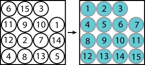
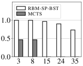
We further compare the performance of RBM-SP-BST and MCTS in lattice rearrangement problems, which are recently studied in the literature [77]. An example with 15 objects is shown in Fig. 28[left]. In the start and goal arrangements, gaps between adjacent objects are set to be 0.01 object radius, and thus buffer allocation is challenging for sampling-based methods. While MCTS tries all the actions on each node, RBM-SP-BST is able to detect the embedded combinatorial object relationship via the dependency graph and therefore needs fewer buffer allocation calls. As shown in Fig. 28[right], RBM-SP-BST has a much higher success rate in lattice rearrangement tasks.

Figure 28: Comparison among methods in lattice instances with 3-35 objects. [left] lattice example; [right] success rate

Figure 29: [Left] “dense-small” instances where 5-8 cylinders packed in the environment and density level $\rho=0.5$. [Right] 10 cuboids with $\rho=0.4$.

8.4.3 Cuboid Objects

Because the MCTS solver only supports cylindrical objects, we only compare RBM-SP-BST and BiRRT(fmRS) in the cuboid setup (Fig. 29[right]). When $\rho=0.3$, RBM-SP-BST computes high-quality solutions efficiently, while BiRRT(fmRS) can only solve instances with up to 20 cuboids. We mention that, when $\rho=0.4$, BiRRT(fmRS) cannot solve any instance, but RBM-SP-BST can solve 50-object rearrangement problems in 28.6 secs on average.

Figure 30: Comparison between methods in cuboid instances with $10$-$30$ cuboids and $\rho=0.3$ (left: computation time in seconds; middle: success rate; right: number of actions as multiples of $|\mathcal{O}|$).

9 Physical Experiments

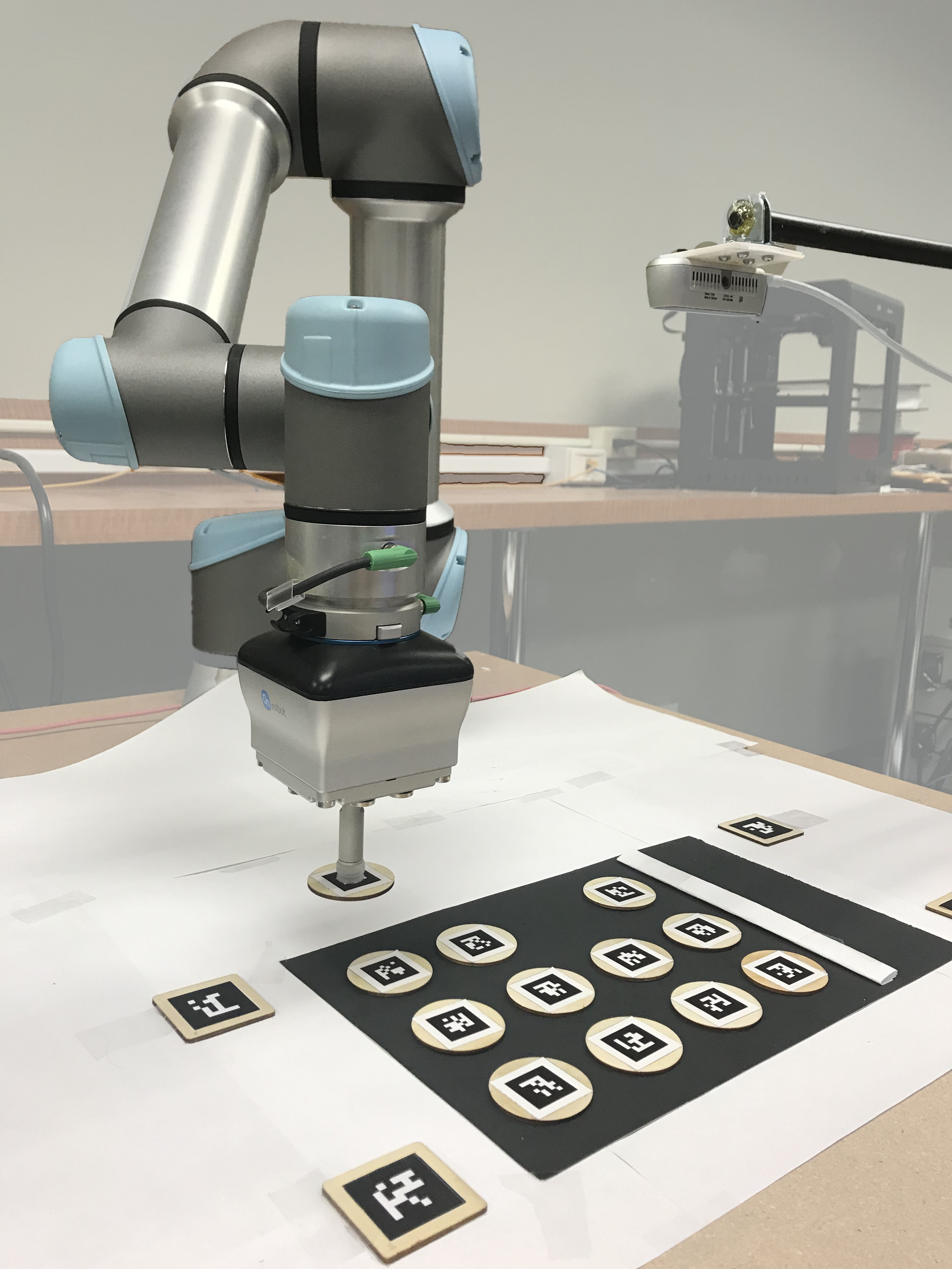
In this section, we demonstrate that the plans computed by proposed algorithms can be readily executed on real robots in a complete vision-planning-control pipeline. We first introduce the hardware setup and the pipeline during the execution of the rearrangement plans. After that, we present experimental results based on the execution of computed rearrangement plans.

9.1 Hardware Setup

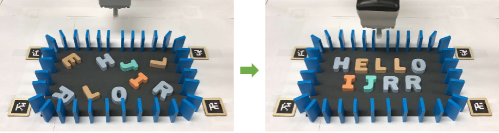
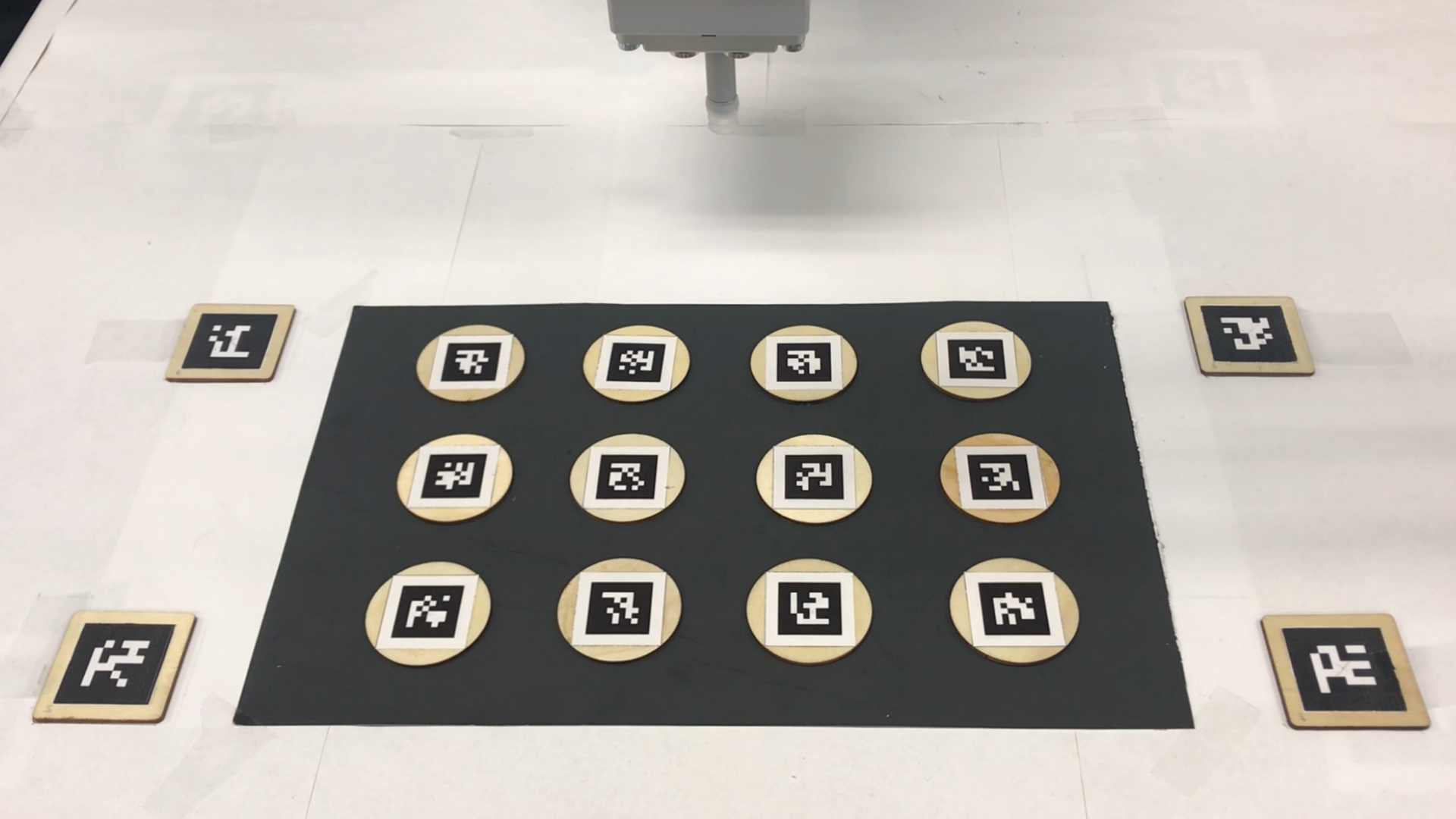
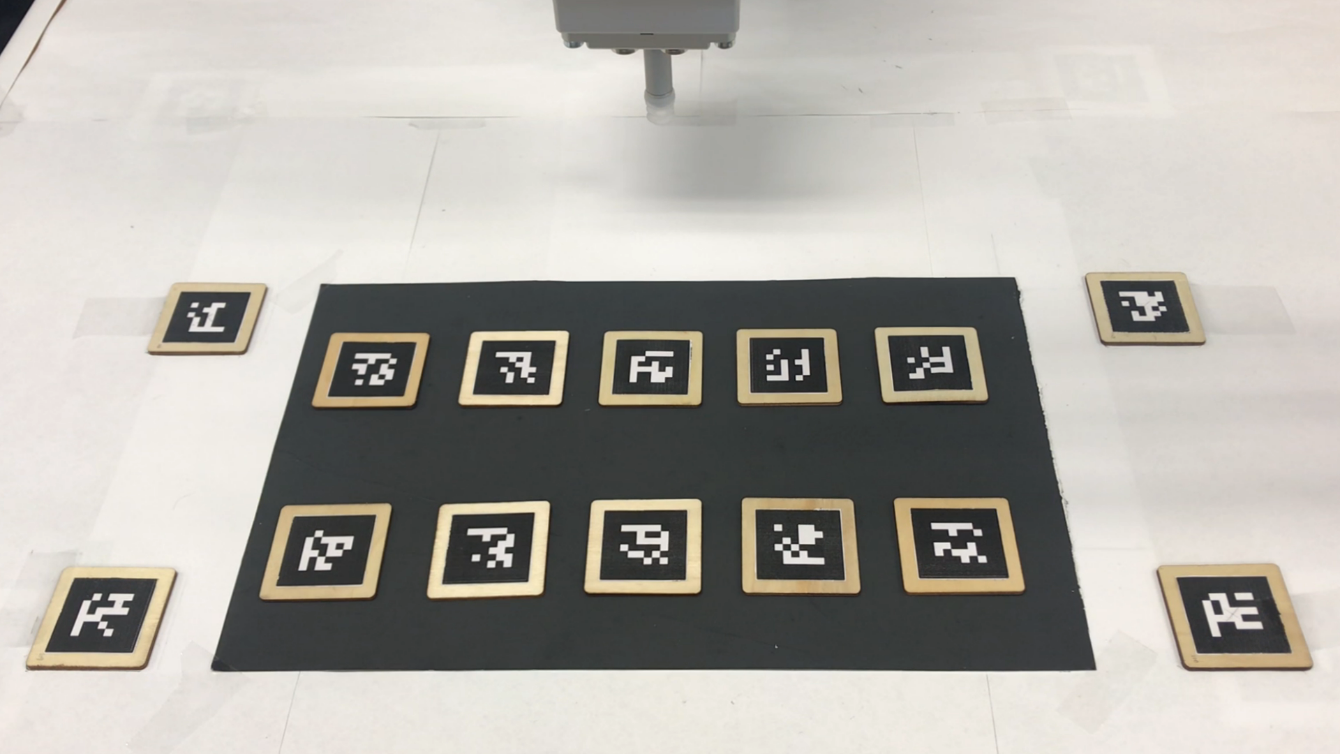
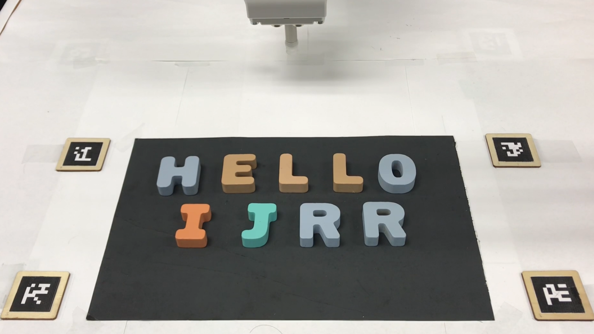
In our hardware setup (Fig.31), we use a UR-5e robot arm with an OnRobot VGC 10 vacuum gripper to execute pick-n-places. An Intel RealSense D435 RGB-D camera is set up above the environment to provide an overview of the entire workspace. The camera calibration is done with four 2D fiducial markers at the corners of the environment using a C++ cross-platform software library Chilitags [78]. In the real robot evaluation, we attempt three scenarios, which are presented in Fig. 32. For both cylindrical objects and cuboid objects, pose estimation is conducted with the aid of Chilitags. For letter objects, the poses are estimated with a deep learning model Mask R-CNN [79]: Given an overview image of the workspace, a pre-trained Mask R-CNN model provides masks of the workspace objects. The 2d pose of each object is obtained by computing a rigid transformation between the detected 2d point cloud and the model point cloud of the object.

Figure 31: Our hardware setup for executing rearrangement plans computed by proposed algorithms.

Figure 32: Three attempted scenarios in the hardware platform: cylindrical scenario (Left), cuboid scenario (Middle), letters (Right)

Input : $\mathcal{A}_{g}$: goal arrangement

1 $\mathcal{A}_{c}\leftarrow PoseEstimation()$

2 $\pi\leftarrow$ RearrangementSolver($\mathcal{A}_{c}$, $\mathcal{A}_{g}$)

3 for ($o$, $p_{c}$, $p_{t}$) in $\pi$ do

4       $p_{c}\leftarrow$ UpdatePose($o$)

5       ExecuteAction(($o$, $p_{c}$, $p_{t}$))

6      

7 end for

8

Algorithm 7 Rearrangement Pipeline

The rearrangement pipeline is shown in Algo. 7. The system first estimates the current poses of workspace objects $\mathcal{A}_{c}$ (Line 1). Given the current arrangement $\mathcal{A}_{c}$ and goal arrangement $\mathcal{A}_{g}$, the rearrangement solver computes a rearrangement plan $\pi$ (Line 2). Each action in $\pi$ consists of three components: manipulating object $o$, current pose $p_{c}$, and target pose $p_{t}$ (Line 3). To improve the accuracy of pick-n-places, we update the grasping pose before each grasp (Line 4-5).

9.2 Experimental Validation

We conduct hardware experiments on TORE, comparing the execution time of RBM plans and TBM plans. With the same notations as those in Sec. 8, RBM plans minimize running buffer size and TBM plans minimize total buffer size. In TORE, minimizing the total buffer size is equivalent to minimizing the number of total actions. An example instance of our experiment is shown in Fig. 33. The right side of the pad works as an external space for buffer placements. We tried 10 instances with 12 cylindrical objects. The results are shown in Tab. 4. While minimizing running buffer size, RBM plans are only 5$\%$ longer than TBM plans on average.

Figure 33: An example instance of our experiment. The right side of the pad works as an external space for buffer placements.

Table 4: Comparison between RBM plans and TBM plans in execution time and the number of actions.

instance	RBM		TBM
	execution time (secs)	# actions	execution time (secs)	# actions
1	211.35	15	194.52	14
2	197.76	14	197.66	14
3	184.49	13	185.82	13
4	201.32	14	205.96	14
5	227.03	16	195.44	14
6	193.84	14	192.61	14
7	216.49	15	198.90	14
8	250.13	17	211.15	15
9	176.75	13	179.83	13
10	179.07	12	160.96	12
Average	203.82	14.3	192.28	13.7

Besides the comparison in TORE, we also compare TORI algorithms in the hardware system. As shown in the accompanying video, TRLB solves all attempted instances, which involve concave objects, in an apparently natural and efficient manner.

10 Conclusions

In this work, we investigate the problem of minimizing the number of running buffers (MRB) for solving labeled and unlabeled tabletop rearrangement problems with overhand grasps (TORO), which translates to finding a best linear ordering of vertices of the associated underlying dependency graph. For TORO, MRB is an important quantity to understand as it determines the problem’s feasibility if only external buffers are to be used, which is the case in some real-world applications [1]. Despite the provably high computational complexity that is involved, we provide effective dynamic programming-based algorithms capable of quickly computing MRB for large and dense labeled/unlabeled TORO instances. In addition, we also provide methods for minimizing the total number of buffers subject to MRB constraints. Whereas we prove that MRB can grow unbounded for both labeled and unlabeled settings for special cases for uniform cylinders, empirical evaluations suggest that real-world random TORO instances are likely to have much smaller MRB values. We demonstrate MRB’s high utility in solving real tabletop rearrangement problems in a bounded, constrained workspace.

We conclude by leaving the readers with some interesting open problems. On the structural side, while LRBM, in general, is proven to be NP-Hard, the computational the intractability of either LRBM with uniform cylinders or URBM in general remains unresolved. As for bounds, the lower and upper bounds of MRB for LRBM for uniform cylinders do not yet agree; can the bound gap be narrowed further? Objects may have different sizes. An interesting question here is if we can move a large object to buffer or a small object to buffer, which is more beneficial? Moving larger objects are more challenging but we may need to do this fewer times.

Appendix

Properties of Unlabeled Dependency Graphs for Special TORO Settings

Proof of Proposition 2.

The maximum degree of the dependency graph is equal to the maximum number of disjoint objects that one object can overlap with. In this proof, we evaluate the upper bound of the maximum overlaps with a disc packing problem. We first discuss the range of distance between two overlapping regular polygons when they are overlapping and disjoint. After that, we relate the problem to a disc packing problem and derive the upper bound. Without loss of generality, we assume the radius of the regular polygons to be 1. When two $d$-sided regular polygons overlap, the distance between the polygon centers is upper bounded by two times the radius of their circumscribed circles, i.e. 2. When two $d$-sided regular polygons are disjoint, the distance between the polygon centers is lower bounded by two times the radius of their inscribed circles, i.e. $2\cos(\dfrac{\pi}{d})$. Due to the mentioned upper bound, the number of disjoint d-sided regular polygons that overlap with one d-sided regular polygon is upper bounded by that whose centers are inside a 2-circle (Fig. 34(a)). Additionally, due to the mentioned distance lower bound, this number is upper bounded by the number of disjoint $\cos(\dfrac{\pi}{d})$-circles whose centers are inside a 2-circle (Fig. 34(b)), which is equal to the number of $\cos(\dfrac{\pi}{d})$-circles packed inside a $(2+\cos(\dfrac{\pi}{d}))$-circle (Fig. 34(c)). Since the radius ratio of circles $\dfrac{2+\cos(\dfrac{\pi}{d})}{\cos(\dfrac{\pi}{d})}$ is upper bounded by 5 when $d\geq 3$, there are at most 19 small circles packed in the large circle [80]. Therefore, the maximum degree of the unlabeled dependency graph is upper bounded by 19. ∎

Proof of Proposition 3.

Constructing the dependency graph based on the start and goal positions in the workspace, the planarity can be proven if no two edges cross each other. Assuming the contrary, there are two edges crossing each other, e.g. $AD$ and $BC$ in Fig. 35[Left]. Since each edge comes from a pair of intersecting start and goal objects, without loss of generality, we can assume $C$, $D$ are start positions and $A$, $B$ are goal positions. Therefore, we have $|AB|,|CD|\geq 2r$, where $r$ is the base radius of the cylinders. Since $AD$ and $BC$ are both connected in the dependency graph, we have $|AD|,|BC|<2r$, which leads to the conclusion that $|AD|+|BC|<4r\leq|AB|+|CD|$, and contradicts the triangle inequality. Therefore, the planarity is proven with contradiction.

Since uniform cylinders have uniform disc bases, one cylinder may only touch six non-overlapping cylinders and non-trivially intersect at most five non-overlapping cylinders. Therefore, the maximum degree of the unlabeled dependency graph is upper bounded by 5. ∎

Figure 34: (a) The number of disjoint d-sided regular polygons that overlap with one d-sided regular polygon is upper bounded by that whose centers are inside a 2-circle. (b) The number of disjoint d-sided regular polygons whose centers are inside a 2-circle is upper bounded by the number of disjoint $\cos(\dfrac{\pi}{d})$-circles whose centers are inside a 2-circle. (c) The number of disjoint $\cos(\dfrac{\pi}{d})$-circles whose centers are inside a 2-circle is equal to the number of $\cos(\dfrac{\pi}{d})$-circles packed inside a $(2+\cos(\dfrac{\pi}{d}))$-circle.

Figure 35: [Left] A case discussed in Prop.3 [Right] A counterexample of the proof of Prop.3 when the base of workspace objects is square.

Remark.

As shown in Fig. 35[Right], the proof of the planarity in Proposition 3 does not hold for objects with regular polygon bases.

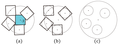
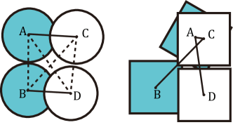
$\Omega(\sqrt{n})$ Lower Bound for URBM

Let $(x,y)$ be the coordinate of a vertex $v_{x,y}$ on $\mathcal{D}(w,h)$ with the top left being $(1,1)$. The parity of $x+y$ determines the partite set of the vertex (recall that unlabeled dependency graph for uniform cylinders is always a planar bipartite graph, by Proposition 3), which may correspond to a start pose or a goal pose. With this in mind, we simply call vertices of $\mathcal{D}(w,h)$ start and goal vertices; without loss of generality, let $v_{1,1}$ be a start vertex.

We use $\mathcal{D}(m,2m)$ for establishing the lower bound on MRB. We use a vertex pair $p_{i,j}$ to refer to two adjacent vertices $v_{i,2j-1}$ and $v_{i,2j}$ in $\mathcal{D}(m,2m)$. It is clear that a vertex pair contains a start and a goal vertex. We say that a goal vertex is filled if an object is placed at the corresponding goal pose. We say that a start vertex (which belongs to a vertex pair) is cleared if the corresponding object at the vertex is picked (either put at a goal or at a buffer) but the corresponding goal in the vertex pair is unfilled. At any moment when the robot is not holding an object, the number of objects in the buffer is the same as the number of cleared vertices. For each column $i,1\leq i\leq m$, let $f_{i}$ (resp., $c_{i}$) be the number of goals (resp., start) vertices in the column that are filled (resp., cleared). Notice that a goal cannot be filled until the object at the corresponding start vertex is removed.

Lemma 3.

On a dependency grid $\mathcal{D}(m,2m)$, for two adjacent columns $i$ and $i+1$, $1\leq i<m$, if $f_{i}+f_{i+1}\neq 0$ or $2m$, then $c_{i}+c_{i+1}\geq 1$. In other words, there is at least one cleared vertex in the two adjacent columns unless $f_{i}=f_{i+1}=0$ or $f_{i}=f_{i+1}=m$.

Proof.

If there is a $j,1\leq j\leq m$, such that only one of the goal vertices in vertex pairs $p_{i,j}$ and $p_{i+1,j}$ is filled (Fig. 36(a)), then the start vertex in the other vertex pair must be cleared. Therefore, $c_{i}+c_{i+1}\geq 1$.

On the other hand, if, for each $j,1\leq j\leq m$, both or neither of the goal vertices in $p_{i,j}$ and $p_{i+1,j}$ is filled, then there is a $j,1\leq j\leq m-1$, such that both goal vertices in $p_{i,j}$ and $p_{i+1,j}$ are filled but neither of those in $p_{i,j+1}$ and $p_{i+1,j+1}$ is filled (Fig. 36(b)) or the opposite (Fig. 36(c)). Then, for the vertex pairs whose goal vertices are not filled, say $p_{i,j+1}$ and $p_{i+1,j+1}$, one of their start vertices is a neighbor of the filled goal in $p_{i,j}$ and $p_{i,j+1}$. Therefore, at least one of the start vertices in $p_{i,j+1}$ and $p_{i+1,j+1}$ is a cleared vertex. And thus, $c_{i}+c_{i+1}\geq 1$.

\begin{overpic}[width=130.08731pt]{figures/lemma_cases-eps-converted-to.pdf} \put(0.0,38.0){{\small$p_{i,j}$}} \put(11.0,38.0){{\small$p_{i+1,j}$}} \par\put(37.0,51.0){{\small$p_{i,j}$}} \put(49.0,51.0){{\small$p_{i+1,j}$}} \put(34.0,-3.0){{\small$p_{i,j+1}$}} \par\put(89.0,51.0){{\small$p_{i+1,j}$}} \put(70.0,-3.0){{\small$p_{i,j+1}$}} \put(89.0,-3.0){{\small$p_{i+1,j+1}$}} \par\put(8.0,-11.5){{\small$(a)$}} \put(44.0,-11.5){{\small$(b)$}} \put(85.0,-11.5){{\small$(c)$}} \end{overpic}

Figure 36: Some cases discussed in the lemma 3. The unshaded and shaded nodes represent the start and goal vertices in the dependency graph. Specifically, the shaded nodes with a dot inside represent the filled vertices and the unshaded nodes with a cross inside represent the cleared vertices. (a) When only one goal vertex in $p_{i,j}$ and $p_{i+1,j}$ is filled up, the start vertex in the other vertex pair is a cleared vertex. (b) When both goal vertices in $p_{i,j}$ and $p_{i+1,j}$ are filled but neither of those in $p_{i,j+1}$ and $p_{i+1,j+1}$ is filled, one of the start vertices $p_{i,j+1}$ and $p_{i+1,j+1}$ is a cleared vertex. (c) The opposite case of (b).

∎

Proof of Lemma 2.

We show that there are $\Omega(m)$ cleared vertices when $\lfloor n/3\rfloor$ goal vertices are filled. Suppose there are $q$ columns in $\mathcal{D}$ with $1\leq f_{i}\leq m-1$. According to the definition of $f_{i}$, for each of these $q$ columns, there is at least one goal vertex that is filled and at least one goal vertex that is not.

If $q<\dfrac{\lfloor n/3\rfloor}{3(m-1)}$, then there are two columns $i$ and $j$, such that $f_{i}=m$ and $f_{j}=0$. That is because $\sum_{1\leq i\leq m}f_{i}=\lfloor n/3\rfloor$ and $0\leq f_{i}\leq m$ for all $1\leq i\leq m$. Therefore, for the vertex pairs in each row $j$, at least one goal vertex is filled but at least one is not. And thus, for each $j$, there are two adjacent columns $i,i+1,1\leq i<m$, such that in vertex pairs $p_{i,j}$ and $p_{i+1,j}$, one goal vertex is filled while the start vertex in the other vertex pair is cleared (Fig. 36(a)). Therefore, there are at least $m$ cleared vertices in this case.

If $q\geq\dfrac{\lfloor n/3\rfloor}{3(m-1)}$, then we partition all the columns in $\mathcal{D}$ into $\lfloor m/2\rfloor$ disjoint pairs: (1,2), (3,4), … The $q$ columns belong to at least $\lfloor q/2\rfloor$ pairs of adjacent columns. Therefore, according to Lemma 3, we have $\Theta(m)$ cleared vertices.

In conclusion, there are $\Omega(m)$ cleared vertices when there are $\lfloor n/3\rfloor$ filled goal. Therefore, the minimum MRB of this instance is $\Omega(m)$. ∎

$O(\sqrt{n})$ Algorithmic Upper Bound for URBM

To investigate the running buffer size of the plan computed by SepPlan, we construct a binary tree $T$ based on SepPlan (Fig. 13(c)). Each node represents a recursive call consuming a subgraph $G^{\,u}(V,E)$ and the left and right children of the node are induced from subgraphs $G^{\,u}(A^{\prime},E(A^{\prime}))$ and $G^{\,u}(B^{\prime},E(B^{\prime}))$ of $G^{\,u}(V,E)$. SepPlan computes the plan by visiting the binary tree in a depth-first manner. For each node on $T$, given the input dependency graph $G^{\,u}(V,E)$, denote the sequence before we deal with $G^{\,u}(V,E)$ as $\pi_{0}$. Denote the vertices pruned in RemovalTrivialGoals( $G^{\,u}(V,E)$) as $P$. Without loss of generality, assume that SepPlan recurses into $A^{\prime}$ before $B^{\prime}$. Let $\pi_{P}$, $\pi_{C^{\prime}}$, $\pi_{A^{\prime}}$, and $\pi_{B^{\prime}}$ be the goal removal sequence after we remove vertices in $P$, $C^{\prime}$, $A^{\prime}$ and $B^{\prime}$ from $G^{\,u}(V,E)$ respectively. We define function $RB(\pi)$ to represent “generalized” current running buffer size of a removal sequence $\pi$: When vertices in $\pi$ are removed from the dependency graph, $RB(\pi)$ equals either the number of running buffers; or the negation of the number of empty goal poses. In the depth-first recursion, each node on the binary tree $T$ is visited at most three times:

1. Before exploring child nodes. The peak may be reached during the removal of $C^{\prime}$. Let $\pi_{C^{*}}$ be the sequence when the running buffer size reaches the peak. $RB(\pi_{C^{*}})\leq RB(\pi_{0})+10\sqrt{2}\sqrt{|V|}$.

2. After we deal with $A^{\prime}$ and before we deal with $B^{\prime}$. $RB(\pi_{A^{\prime}})=RB(\pi_{0})$$-\delta(C^{\prime})-\delta(A^{\prime})$.

3. After we deal with $B^{\prime}$. $RB(\pi_{B^{\prime}})=RB(\pi_{0})$$-\delta(V)$.

Lemma 4.

$RB(\pi_{A^{\prime}})\leq(RB(\pi_{C^{*}})+RB(\pi_{B^{\prime}}))/2$.

Proof.

$$\begin{split}&RB(\pi_{A^{\prime}})\\ &=RB(\pi_{0})-\delta{P}-\delta{C^{\prime}}-\delta{A^{\prime}}\\ &=RB(\pi_{0})-\delta(P)-\delta(C^{\prime})-\max[\delta(A^{\prime}),\delta(B^{\prime})]\\ &\leq RB(\pi_{0})-\delta(P)-\delta(C^{\prime})+\dfrac{1}{2}[-\delta(V)+\delta(P)+\delta(C^{\prime})]\\ &=\dfrac{1}{2}\{[RB(\pi_{0})-\delta(V)]+[RB(\pi_{0})-\delta(P)-\delta(C^{\prime})]\}\\ &=\dfrac{1}{2}[RB(\pi_{B^{\prime}})+RB(\pi_{C^{\prime}})]\\ &\leq\dfrac{1}{2}[RB(\pi_{B^{\prime}})+RB(\pi_{C^{*}})]\end{split}$$

∎

Lemma 4 establishes the relationship among $\pi_{C^{*}}$, $\pi_{A^{\prime}}$, and $\pi_{B^{\prime}}$ of a node on $T$. With this lemma, we obtain an upper bound for each node:

Lemma 5.

Given a node $N$ with depth $d$ in the binary tree $T$, let $\pi_{C^{*}}(N)$, $\pi_{A^{\prime}}(N)$, and $\pi_{B^{\prime}}(N)$ be $\pi_{C^{*}}$, $\pi_{A^{\prime}}$, and $\pi_{B^{\prime}}$ of $N$ respectively. $RB(\pi_{C^{*}}(N))$, $RB(\pi_{A^{\prime}}(N))$, and $RB(\pi_{B^{\prime}}(N))$ are all upper bounded by

$$\dfrac{[1-(\sqrt{\dfrac{2}{3}})^{d+1}]}{1-\sqrt{\dfrac{2}{3}}}20\sqrt{n}$$ (10)

where $n$ is the number of objects in the instance.

Proof.

The conclusion can be proven by induction.

When $d=0$, the dependency graph at the root node $r$ has $n$ start vertices and $n$ goal vertices. We have $RB(\pi_{C^{*}})\leq 20\sqrt{n},RB(\pi_{B^{\prime}})=0$. According to Lemma 4, $RB(\pi_{A^{\prime}})\leq 10\sqrt{n}$. The conclusion holds.

Assume that the conclusion holds for all the nodes with depth less than or equal to $k$. Given an arbitrary node $N$ in the depth $k$, let the left and right children of $N$ be $L$ and $R$, which are the nodes with depth $k+1$. The corresponding dependency graphs have at most $(2/3)^{k+1}\cdot 2n$ vertices respectively.

$$RB(\pi_{C^{*}}(L))\leq RB(\pi_{C^{*}}(N))+\sqrt{(2/3)^{k+1}\cdot 2n}\cdot 10\sqrt{2}$$

$$RB(\pi_{C^{*}}(R))\leq RB(\pi_{A^{\prime}}(N))+\sqrt{(2/3)^{k+1}\cdot 2n}\cdot 10\sqrt{2}$$

Since $\pi_{B^{\prime}}(L)=\pi_{A^{\prime}}(N)$ and $\pi_{B^{\prime}}(R)=\pi_{B^{\prime}}(N)$, upper bound for nodes with depth $k$ holds for $\pi_{B^{\prime}}(L)$ and $\pi_{B^{\prime}}(R)$. Therefore, the running buffer size for the depth $k+1$ nodes has an upper bound

$$\begin{split}&\dfrac{[1-(\sqrt{2/3})^{k+1}]}{1-\sqrt{2/3}}20\sqrt{n}+\sqrt{(2/3)^{k+1}\cdot 2n}\cdot 10\sqrt{2}\\ =&\dfrac{[1-(\sqrt{2/3})^{k+2}]}{1-\sqrt{2/3}}20\sqrt{n}\end{split}$$ (11)

Therefore, the upper bound holds for all the nodes of depth $k+1$. With induction, the lemma holds. ∎

With Lemma 5, it is straightforward to establish that MRB is bounded by $\dfrac{20}{1-\sqrt{2/3}}\sqrt{n}$, yielding Theorem 4.

References

- [1] S. D. Han, N. M. Stiffler, A. Krontiris, K. E. Bekris, and J. Yu, “Complexity results and fast methods for optimal tabletop rearrangement with overhand grasps,” The International Journal of Robotics Research, vol. 37, no. 13-14, pp. 1775–1795, 2018.
- [2] K. Gao, S. W. Feng, and J. Yu, “On minimizing the number of running buffers for tabletop rearrangement,” in Robotics: Sciences and Systems, 2021.
- [3] K. Gao, D. Lau, B. Huang, K. E. Bekris, and J. Yu, “Fast high-quality tabletop rearrangement in bounded workspace,” in 2022 International Conference on Robotics and Automation (ICRA), pp. 1961–1967, 2022.
- [4] A. Saxena, J. Driemeyer, and A. Y. Ng, “Robotic grasping of novel objects using vision,” The International Journal of Robotics Research, vol. 27, no. 2, pp. 157–173, 2008.
- [5] M. Gualtieri, A. Ten Pas, K. Saenko, and R. Platt, “High precision grasp pose detection in dense clutter,” in 2016 IEEE/RSJ International Conference on Intelligent Robots and Systems (IROS), pp. 598–605, IEEE, 2016.
- [6] C. Mitash, K. E. Bekris, and A. Boularias, “A self-supervised learning system for object detection using physics simulation and multi-view pose estimation,” in 2017 IEEE/RSJ International Conference on Intelligent Robots and Systems (IROS), pp. 545–551, IEEE, 2017.
- [7] Y. Xiang, T. Schmidt, V. Narayanan, and D. Fox, “Posecnn: A convolutional neural network for 6d object pose estimation in cluttered scenes,” in Robotics: Science and Systems, 2018.
- [8] M. Stilman and J. J. Kuffner, “Navigation among movable obstacles: Real-time reasoning in complex environments,” International Journal of Humanoid Robotics, vol. 2, no. 04, pp. 479–503, 2005.
- [9] K. Treleaven, M. Pavone, and E. Frazzoli, “Asymptotically optimal algorithms for one-to-one pickup and delivery problems with applications to transportation systems,” IEEE Transactions on Automatic Control, vol. 58, no. 9, pp. 2261–2276, 2013.
- [10] G. Havur, G. Ozbilgin, E. Erdem, and V. Patoglu, “Geometric rearrangement of multiple movable objects on cluttered surfaces: A hybrid reasoning approach,” in 2014 IEEE International Conference on Robotics and Automation (ICRA), pp. 445–452, IEEE, 2014.
- [11] A. Krontiris and K. E. Bekris, “Dealing with difficult instances of object rearrangement.,” in Robotics: Science and Systems, vol. 1123, 2015.
- [12] J. E. King, M. Cognetti, and S. S. Srinivasa, “Rearrangement planning using object-centric and robot-centric action spaces,” in 2016 IEEE International Conference on Robotics and Automation (ICRA), pp. 3940–3947, IEEE, 2016.
- [13] J. Lee, Y. Cho, C. Nam, J. Park, and C. Kim, “Efficient obstacle rearrangement for object manipulation tasks in cluttered environments,” in 2019 International Conference on Robotics and Automation (ICRA), pp. 183–189, IEEE, 2019.
- [14] R. H. Taylor, M. T. Mason, and K. Y. Goldberg, “Sensor-based manipulation planning as a game with nature,” in Fourth International Symposium on Robotics Research, pp. 421–429, 1987.
- [15] K. Y. Goldberg, “Orienting polygonal parts without sensors,” Algorithmica, vol. 10, no. 2, pp. 201–225, 1993.
- [16] K. M. Lynch and M. T. Mason, “Dynamic nonprehensile manipulation: Controllability, planning, and experiments,” The International Journal of Robotics Research, vol. 18, no. 1, pp. 64–92, 1999.
- [17] M. Dogar and S. Srinivasa, “A framework for push-grasping in clutter,” Robotics: Science and systems VII, vol. 1, 2011.
- [18] J. Bohg, A. Morales, T. Asfour, and D. Kragic, “Data-driven grasp synthesis—a survey,” IEEE Transactions on Robotics, vol. 30, no. 2, pp. 289–309, 2013.
- [19] N. C. Dafle, A. Rodriguez, R. Paolini, B. Tang, S. S. Srinivasa, M. Erdmann, M. T. Mason, I. Lundberg, H. Staab, and T. Fuhlbrigge, “Extrinsic dexterity: In-hand manipulation with external forces,” in 2014 IEEE International Conference on Robotics and Automation (ICRA), pp. 1578–1585, IEEE, 2014.
- [20] A. Boularias, J. A. Bagnell, and A. Stentz, “Learning to manipulate unknown objects in clutter by reinforcement,” in 29th AAAI Conference on Artificial Intelligence, AAAI 2015 and the 27th Innovative Applications of Artificial Intelligence Conference, IAAI 2015, pp. 1336–1342, AI Access Foundation, 2015.
- [21] N. Chavan-Dafle and A. Rodriguez, “Prehensile pushing: In-hand manipulation with push-primitives,” in 2015 IEEE/RSJ International Conference on Intelligent Robots and Systems (IROS), pp. 6215–6222, IEEE, 2015.
- [22] L. P. Kaelbling and T. Lozano-Pérez, “Hierarchical task and motion planning in the now,” in 2011 IEEE International Conference on Robotics and Automation, pp. 1470–1477, IEEE, 2011.
- [23] S. Levine, C. Finn, T. Darrell, and P. Abbeel, “End-to-end training of deep visuomotor policies,” The Journal of Machine Learning Research, vol. 17, no. 1, pp. 1334–1373, 2016.
- [24] J. Mahler, J. Liang, S. Niyaz, M. Laskey, R. Doan, X. Liu, J. A. Ojea, and K. Goldberg, “Dex-net 2.0: Deep learning to plan robust grasps with synthetic point clouds and analytic grasp metrics,” arXiv preprint arXiv:1703.09312, 2017.
- [25] A. Zeng, S. Song, K.-T. Yu, E. Donlon, F. R. Hogan, M. Bauza, D. Ma, O. Taylor, M. Liu, E. Romo, et al., “Robotic pick-and-place of novel objects in clutter with multi-affordance grasping and cross-domain image matching,” in 2018 IEEE international conference on robotics and automation (ICRA), pp. 3750–3757, IEEE, 2018.
- [26] A. M. Wells, N. T. Dantam, A. Shrivastava, and L. E. Kavraki, “Learning feasibility for task and motion planning in tabletop environments,” IEEE robotics and automation letters, vol. 4, no. 2, pp. 1255–1262, 2019.
- [27] J. E. Hopcroft, J. T. Schwartz, and M. Sharir, “On the complexity of motion planning for multiple independent objects; pspace-hardness of the ‘warehouseman’s problem’,” The International Journal of Robotics Research, vol. 3, no. 4, pp. 76–88, 1984.
- [28] G. Wilfong, “Motion planning in the presence of movable obstacles,” Annals of Mathematics and Artificial Intelligence, vol. 3, no. 1, pp. 131–150, 1991.
- [29] M. Stilman, J.-U. Schamburek, J. Kuffner, and T. Asfour, “Manipulation planning among movable obstacles,” in Proceedings 2007 IEEE international conference on robotics and automation, pp. 3327–3332, IEEE, 2007.
- [30] R. Wang, K. Gao, J. Yu, and K. Bekris, “Lazy rearrangement planning in confined spaces,” in Proceedings of the International Conference on Automated Planning and Scheduling, vol. 32, pp. 385–393, 2022.
- [31] C. H. Papadimitriou, “The euclidean travelling salesman problem is np-complete,” Theoretical computer science, vol. 4, no. 3, pp. 237–244, 1977.
- [32] R. M. Karp, “Reducibility among combinatorial problems,” in Complexity of computer computations, pp. 85–103, Springer, 1972.
- [33] S. Bereg and A. Dumitrescu, “The lifting model for reconfiguration,” Discrete & Computational Geometry, vol. 35, no. 4, pp. 653–669, 2006.
- [34] C. Nam, J. Lee, Y. Cho, J. Lee, D. H. Kim, and C. Kim, “Planning for target retrieval using a robotic manipulator in cluttered and occluded environments,” arXiv preprint arXiv:1907.03956, 2019.
- [35] D. Halperin, M. van Kreveld, G. Miglioli-Levy, and M. Sharir, “Space-aware reconfiguration,” arXiv preprint arXiv:2006.04402, 2020.
- [36] O. Ben-Shahar and E. Rivlin, “Practical pushing planning for rearrangement tasks,” IEEE Transactions on Robotics and Automation, vol. 14, no. 4, pp. 549–565, 1998.
- [37] E. Huang, Z. Jia, and M. T. Mason, “Large-scale multi-object rearrangement,” in 2019 International Conference on Robotics and Automation (ICRA), pp. 211–218, IEEE, 2019.
- [38] L. Chang, J. R. Smith, and D. Fox, “Interactive singulation of objects from a pile,” in 2012 IEEE International Conference on Robotics and Automation, pp. 3875–3882, IEEE, 2012.
- [39] M. Laskey, J. Lee, C. Chuck, D. Gealy, W. Hsieh, F. T. Pokorny, A. D. Dragan, and K. Goldberg, “Robot grasping in clutter: Using a hierarchy of supervisors for learning from demonstrations,” in 2016 IEEE International Conference on Automation Science and Engineering (CASE), pp. 827–834, IEEE, 2016.
- [40] A. Eitel, N. Hauff, and W. Burgard, “Learning to singulate objects using a push proposal network,” in Robotics research, pp. 405–419, Springer, 2020.
- [41] H. Song, J. A. Haustein, W. Yuan, K. Hang, M. Y. Wang, D. Kragic, and J. A. Stork, “Multi-object rearrangement with monte carlo tree search: A case study on planar nonprehensile sorting,” arXiv:1912.07024, 2019.
- [42] Z. Pan and K. Hauser, “Decision making in joint push-grasp action space for large-scale object sorting,” arXiv preprint arXiv:2010.10064, 2020.
- [43] A. Zeng, S. Song, S. Welker, J. Lee, A. Rodriguez, and T. Funkhouser, “Learning synergies between pushing and grasping with self-supervised deep reinforcement learning,” in 2018 IEEE/RSJ International Conference on Intelligent Robots and Systems (IROS), pp. 4238–4245, IEEE, 2018.
- [44] B. Huang, S. D. Han, A. Boularias, and J. Yu, “DIPN: Deep Interaction Prediction Network with Application to Clutter Removal,” in IEEE International Conference on Robotics and Automation (ICRA), 2021.
- [45] B. Huang, S. D. Han, J. Yu, and A. Boularias, “Visual foresight tree for object retrieval from clutter with nonprehensile rearrangement,” arXiv preprint arXiv:2105.02857, 2021.
- [46] E. R. Vieira, D. Nakhimovich, K. Gao, R. Wang, J. Yu, and K. E. Bekris, “Persistent homology for effective non-prehensile manipulation,” in 2022 International Conference on Robotics and Automation (ICRA), pp. 1918–1924, IEEE, 2022.
- [47] S. J. Buckley, Fast motion planning for multiple moving robots. IBM Thomas J. Watson Research Division, 1988.
- [48] J. van Den Berg, J. Snoeyink, M. C. Lin, and D. Manocha, “Centralized path planning for multiple robots: Optimal decoupling into sequential plans.,” in Robotics: Science and systems, vol. 2, pp. 2–3, 2009.
- [49] A. Krontiris and K. E. Bekris, “Efficiently solving general rearrangement tasks: A fast extension primitive for an incremental sampling-based planner,” in 2016 IEEE International Conference on Robotics and Automation (ICRA), pp. 3924–3931, IEEE, 2016.
- [50] F. Wang and K. Hauser, “Robot packing with known items and nondeterministic arrival order,” IEEE Transactions on Automation Science and Engineering, 2020.
- [51] K. Gao and J. Yu, “Toward efficient task planning for dual-arm tabletop object rearrangement,” in 2022 IEEE/RSJ International Conference on Intelligent Robots and Systems (IROS), pp. 10425–10431, IEEE, 2022.
- [52] K. Gao and J. Yu, “On the utility of buffers in pick-n-swap based lattice rearrangement,” arXiv preprint arXiv:2209.05390, 2022.
- [53] J. Díaz, J. Petit, and M. Serna, “A survey of graph layout problems,” ACM Computing Surveys (CSUR), vol. 34, no. 3, pp. 313–356, 2002.
- [54] M. R. Garey and D. S. Johnson, Computers and intractability, vol. 174. freeman San Francisco, 1979.
- [55] C. H. Papadimitriou, “The np-completeness of the bandwidth minimization problem,” Computing, vol. 16, no. 3, pp. 263–270, 1976.
- [56] M. R. Garey, D. S. Johnson, and L. Stockmeyer, “Some simplified np-complete problems,” in Proceedings of the sixth annual ACM symposium on Theory of computing, pp. 47–63, 1974.
- [57] F. Gavril, “Some np-complete problems on graphs,” tech. rep., Computer Science Department, Technion, 2011.
- [58] H. L. Bodlaender, J. R. Gilbert, H. Hafsteinsson, and T. Kloks, “Approximating treewidth, pathwidth, frontsize, and shortest elimination tree,” Journal of Algorithms, vol. 18, no. 2, pp. 238–255, 1995.
- [59] T.-h. Shin, H. Oh, and S. Ha, “Minimizing buffer requirements for throughput constrained parallel execution of synchronous dataflow graph,” in 16th Asia and South Pacific Design Automation Conference (ASP-DAC 2011), pp. 165–170, IEEE, 2011.
- [60] R. J. Lipton and R. E. Tarjan, “A separator theorem for planar graphs,” SIAM Journal on Applied Mathematics, vol. 36, no. 2, pp. 177–189, 1979.
- [61] J. R. Gilbert, J. P. Hutchinson, and R. E. Tarjan, “A separator theorem for graphs of bounded genus,” Journal of Algorithms, vol. 5, no. 3, pp. 391–407, 1984.
- [62] N. Alon, P. Seymour, and R. Thomas, “A separator theorem for graphs with an excluded minor and its applications,” in Proceedings of the twenty-second annual ACM symposium on Theory of computing, pp. 293–299, 1990.
- [63] U. Elsner, Graph partitioning-a survey. Techn. Univ., 1997.
- [64] R. Tarjan, “Depth-first search and linear graph algorithms,” SIAM journal on computing, vol. 1, no. 2, pp. 146–160, 1972.
- [65] Y. Shiloach, “A minimum linear arrangement algorithm for undirected trees,” SIAM Journal on Computing, vol. 8, no. 1, pp. 15–32, 1979.
- [66] D. Adolphson and T. C. Hu, “Optimal linear ordering,” SIAM Journal on Applied Mathematics, vol. 25, no. 3, pp. 403–423, 1973.
- [67] L. M. Kirousis and C. H. Papadimitriou, “Searching and pebbling,” Theoretical Computer Science, vol. 47, pp. 205–218, 1986.
- [68] N. G. Kinnersley, “The vertex separation number of a graph equals its path-width,” Information Processing Letters, vol. 42, no. 6, pp. 345–350, 1992.
- [69] M. R. Fellows and M. A. Langston, “On search decision and the efficiency of polynomial-time algorithms,” in Proceedings of the twenty-first annual ACM symposium on Theory of computing, pp. 501–512, 1989.
- [70] B. Monien and I. H. Sudborough, “Min cut is np-complete for edge weighted trees,” Theoretical Computer Science, vol. 58, no. 1-3, pp. 209–229, 1988.
- [71] F. István, “On straight-line representation of planar graphs,” Acta scientiarum mathematicarum, vol. 11, no. 229-233, p. 2, 1948.
- [72] R. Wang, K. Gao, D. Nakhimovich, J. Yu, and K. E. Bekris, “Uniform object rearrangement: From complete monotone primitives to efficient non-monotone informed search,” arXiv preprint arXiv:2101.12241, 2021.
- [73] N. Chernov, Y. Stoyan, and T. Romanova, “Mathematical model and efficient algorithms for object packing problem,” Computational Geometry, vol. 43, no. 5, pp. 535–553, 2010.
- [74] N. Koenig and A. Howard, “Design and use paradigms for gazebo, an open-source multi-robot simulator,” in 2004 IEEE/RSJ International Conference on Intelligent Robots and Systems (IROS)(IEEE Cat. No. 04CH37566), vol. 3, pp. 2149–2154, IEEE, 2004.
- [75] L. Gurobi Optimization, “Gurobi optimizer reference manual,” 2021.
- [76] Y. Labbé, S. Zagoruyko, I. Kalevatykh, I. Laptev, J. Carpentier, M. Aubry, and J. Sivic, “Monte-carlo tree search for efficient visually guided rearrangement planning,” IEEE Robotics and Automation Letters, vol. 5, no. 2, pp. 3715–3722, 2020.
- [77] J. Yu, “Rearrangement on lattices with pic-n-swaps: Optimality structures and efficient algorithms,” in Robotics: Sciences and Systems, 2021.
- [78] Q. Bonnard, S. Lemaignan, G. Zufferey, A. Mazzei, S. Cuendet, N. Li, A. Özgür, and P. Dillenbourg, “Chilitags 2: Robust fiducial markers for augmented reality and robotics.,” 2013.
- [79] K. He, G. Gkioxari, P. Dollár, and R. Girshick, “Mask r-cnn,” in Proceedings of the IEEE international conference on computer vision, pp. 2961–2969, 2017.
- [80] F. Fodor, “The densest packing of 19 congruent circles in a circle,” Geometriae Dedicata, vol. 74, no. 2, pp. 139–145, 1999.