Incorporating Unlabelled Data into
Bayesian Neural Networks

Abstract

Conventional Bayesian Neural Networks (BNNs) cannot leverage unlabelled data to improve their predictions. To overcome this limitation, we introduce Self-Supervised Bayesian Neural Networks, which use unlabelled data to learn improved prior predictive distributions by maximising an evidence lower bound during an unsupervised pre-training step. With a novel methodology developed to better understand prior predictive distributions, we then show that self-supervised prior predictives capture image semantics better than conventional BNN priors. In our empirical evaluations, we see that self-supervised BNNs offer the label efficiency of self-supervised methods and the uncertainty estimates of Bayesian methods, particularly outperforming conventional BNNs in low-to-medium data regimes.

1 Introduction

Bayesian Neural Networks (BNNs) are powerful probabilistic models that combine the flexibility of deep neural networks with the theoretical underpinning of Bayesian methods (Mackay, 1992; Neal, 1995). Indeed, as they place priors over their parameters and perform posterior inference, BNN advocates consider them to be a principled approach for uncertainty estimation (Wilson and Izmailov, 2020; Abdar et al., 2021), which can be helpful for label-efficient learning (Gal et al., 2017).

However, despite the prevalence of unlabelled data and the rise of unsupervised learning, conventional BNNs cannot harness unlabelled data for improved uncertainty estimates and label efficiency. Rather, practitioners have focused on improving label efficiency and predictive performance by imparting information with priors over network parameters or predictive functions (e.g., Louizos et al., 2017; Tran et al., 2020; Matsubara et al., 2021; Fortuin et al., 2021a). But it stands to reason that the vast store of information contained in unlabelled data should be incorporated into BNNs, and that the potential benefit of doing so likely exceeds the benefit of designing better, but ultimately human-specified, priors over parameters or functions. Unfortunately, as standard BNNs are explicitly only models for supervised prediction, they cannot leverage such unlabelled data by conditioning on it.

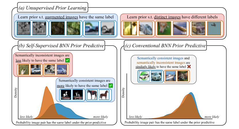
Figure 1: Self-Supervised Bayesian Neural Networks. (a) Pre-training in self-supervised BNNs corresponds to unsupervised prior learning. We learn a prior predictive distribution such that augmented images likely have the same label and distinct images likely have different labels. (b) Self-supervised BNN priors assign higher probabilities to semantically consistent image pairs having the same label compared to semantically inconsistent image pairs. Here, semantically consistent image pairs have the same ground-truth label, and semantically inconsistent image pairs have different ground-truth labels. The plot shows a kernel density estimate of the log-probability that same-class and different-class image pairs are assigned the same label under the prior. (c) Unlike self-supervised prior predictives, conventional BNN prior predictives assign similar probabilities to semantically consistent and semantically inconsistent image pairs having the same label.

To overcome this limitation, we introduce Self-Supervised Bayesian Neural Networks (§3), which condition on pseudo-labelled tasks generated using unlabelled data. We show this can be seen as incorporating unlabelled data into the prior predictive distribution. That is, our method improves the prior predictive by using unlabelled label to learn it, not by using a different but ultimately human-specified prior over parameters or functions. Self-supervised BNNs first train a deterministic encoder to maximise a lower bound of a log-marginal likelihood derived from unlabelled data in the unsupervised pre-training step. Although the encoder is deterministic, it induces a prior predictive distribution over the downstream labels such that augmented image pairs likely have the same label, while distinct images likely have different labels (Fig. 1a). Following the pre-training step, we then condition a subset of the network parameters on the downstream labelled data to make predictions.

As a further contribution, we develop a methodology to better understand prior predictive distributions of functions with high-dimensional inputs (§3). Since it is often easy to reason about the semantic relationship between points, our approach investigates the joint prior predictive for input pairs with known semantic relation. We then demonstrate that self-supervised BNN prior predictives reflect input pair semantic similarity better than normal BNN priors. In particular, while normal BNN priors struggle to distinguish same-class input pairs and different-class input pairs (Fig. 1c), self-supervised BNN priors do so much better (Fig. 1b).

Finally, we demonstrate that the improved prior predictives of self-supervised BNNs are helpful in practice (§4). In our experiments, we find that self-supervised BNNs combine the label efficiency of self-supervised approaches with the uncertainty estimates of Bayesian methods. In particular, self-supervised BNNs outperform conventional BNNs at low-to-medium data regimes in semi-supervised and active learning settings, whilst also offering better-calibrated predictions than SimCLR (Chen et al., 2020a), which is a particularly popular self-supervised learning algorithm.

2 Background: Bayesian Neural Networks

Let $f_{\theta}(x)$ be a neural network with parameters $\theta$ and $\mathcal{D}=\{(x_{i},y_{i})\}_{i=1}^{N}$ be an observed dataset where we want to predict $y$ from $x$. A Bayesian Neural Network (BNN) specifies a prior over parameters, $p(\theta)$, and a likelihood, $p(y|f_{\theta}(x))$, which in turn define the posterior $p(\theta|\mathcal{D})\propto p(\theta)\prod_{i}p(y_{i}|f_{\theta}(x_{i}))$. To make predictions, we approximate the posterior predictive $p(y_{\star}|x_{\star},\mathcal{D})=\mathbb{E}_{p(\theta|\mathcal{D})}[p(y_{\star}|f_{\theta}(x_{\star}))]$.

Improving BNN priors has been a long-standing goal for the BNN community, primarily through improved human-designed priors. One approach is to improve the prior over the network’s parameters (Louizos et al., 2017; Nalisnick, 2018). Others place priors directly over predictive functions (Flam-Shepherd et al., 2017; Sun et al., 2019; Matsubara et al., 2021; Nalisnick et al., 2021; Raj et al., 2023). Both approaches, however, present challenges—the mapping between the network’s parameters and predictive functions is complex, while directly specifying our beliefs over predictive functions is itself a highly challenging task. For these reasons, as well as computational convenience, isotropic Gaussian priors over network parameters remain the most common choice (Fortuin, 2022).

3 Self-Supervised Bayesian Neural Networks

Conventional BNNs are unable to harness unlabelled data for improved uncertainty estimation and label efficiency. To overcome this limitation, we introduce Self-Supervised Bayesian Neural Networks. At a high level, they use unlabelled data and data augmentation to generate pseudo-labelled datasets, which are then conditioned on in a modified probabilistic model.

Problem Specification  Suppose $\mathcal{D}^{u}={\{x^{u}_{i}\}}_{i=1}^{N}$ is an unlabelled dataset of examples $x_{i}^{u}\in\mathbb{R}^{n}$ with $x_{i}\sim P_{X}^{u}$; $P_{X}^{u}$ is the underlying data distribution. Let $\mathcal{D}^{t}=\{(x_{i}^{t},y_{i}^{t})\}_{i=1}^{T}$ be a labelled dataset corresponding to a supervised “downstream” task, where $y_{i}^{t}$ is the target associated with $x_{i}^{t}$. We have $x_{i}\sim P_{X}^{t}$ and $y_{i}|x_{i}\sim P_{Y\text{|}X}^{t}$. We want to use $\mathcal{D}^{u}$ to improve our predictions on the downstream task.

3.1 Incorporating Unlabelled Data into BNNs

The natural way to benefit from $\mathcal{D}^{u}$ would be to use it to inform our beliefs about the model parameters, $\theta$, through the posterior $p(\theta|\mathcal{D}^{u},\mathcal{D}^{t})\propto p(\theta|\mathcal{D}^{u})\,p(\mathcal{D}^{t}|\mathcal{D}^{u},\theta)$. But if we are working with conventional BNNs, which are explicitly models for supervised prediction, $p(\theta|\mathcal{D}^{u})=p(\theta)$. Further, as predictions depend only on the parameters, $p(\mathcal{D}^{t}|\mathcal{D}^{u},\theta)=p(\mathcal{D}^{t}|\theta)$, which then means $p(\theta|\mathcal{D}^{u},\mathcal{D}^{t})=p(\theta|\mathcal{D}^{t})$. Said differently, for a conventional BNN, we cannot incorporate $\mathcal{D}^{u}$ by conditioning on it. One could proceed in different ways, for instance, by using $\mathcal{D}^{u}$ to choose/learn the prior $p(\theta)$, or using a generative model that defines a likelihood for the inputs $p(x|\theta)$.

In this work, we instead note that if we were able to convert $\mathcal{D}^{u}$ into labelled data, we could condition a discriminative model on it. If we then introduced a probabilistic link between generated labelled data, derived from $\mathcal{D}^{u}$, and the predictions over the downstream task labels, we could harness $\mathcal{D}^{u}$ through probabilistic conditioning. We now introduce each of these elements in turn.

First, to generate labelled data from $\mathcal{D}^{u}$, i.e., to formulate self-supervision, we take inspiration from contrastive learning (Oord et al., 2019; Chen et al., 2020b, a; Grill et al., 2020; Hénaff et al., 2020; Chen and He, 2020). We intuitively believe that distinct examples are unlikely to be semantically consistent, and thus are unlikely to have the same downstream label. Further, if we can specify data transformations that preserve semantic information, we also believe that augmented versions of the same example likely have the same downstream label. The correspondence between such beliefs and a prior distribution over predictive functions or network parameters is unclear, so we instead use $\mathcal{D}^{u}$ and data transformations to generate pseudo-labelled data, and include this additional subjective information by conditioning on those datasets rather than a prior over parameters or functions.

Concretely, suppose we have a set of data augmentations $\mathcal{A}=\{a:\mathbb{R}^{n}\rightarrow\mathbb{R}^{n}\}$ that preserve semantic content. We use $\mathcal{A}$ and $\mathcal{D}^{u}$ to generate a contrastive dataset $\mathcal{D}^{c}$ that reflects our subjective beliefs by:

1. Drawing $M$ examples from $\mathcal{D}^{u}$ at random, $\{\hat{x}_{i}\}_{i=1}^{M}$; $i$ indexes the subset, not $\mathcal{D}^{u}$

2. For each $x_{i}$, sampling $a^{A},a^{B}\sim\mathcal{A}$ and augmenting, giving $\tilde{x}_{i}^{A}=a^{A}(\hat{x}_{i})$ and $\tilde{x}_{i}^{B}=a^{B}(\hat{x}_{i})$

3. Forming $\mathcal{D}^{c}$ by assigning $\tilde{x}_{i}^{A}$ and $\tilde{x}_{i}^{B}$ the same class label, which is the subset index $i$

We thus have $\mathcal{D}^{c}=\{(x_{i}^{c},y_{i}^{c})\}_{i=1}^{2M}=\{(\tilde{x}_{i}^{A},i)\}_{i=1}^{M}\cup\{(\tilde{x}_{i}^{B},i)\}_{i=1}^{M}$, where the labels are between $1$ and $M$. The task is to predict the subset index corresponding to each augmented example. We can repeat this process $L$ times and create a set of contrastive task datasets, $\{\mathcal{D}^{c}_{j}\}_{j=1}^{L}$. Here, we consider the number of generated contrastive datasets $L$ to be a fixed, finite hyper-parameter, but we discuss the implications of generating a potentially infinite number of datasets in Appendix A.

Second, to link the labelled data derived from $\mathcal{D}^{u}$ and the downstream task predictions, we use parameter sharing (see Fig. 2). We introduce parameters $\theta_{j}^{c}$ for each $\mathcal{D}^{c}_{j}$, parameters $\theta^{t}$ for $\mathcal{D}^{t}$, and shared-parameters $\theta^{s}$ that are used for both the downstream and the contrastive tasks. A contrastive dataset $\mathcal{D}^{c}_{j}$ thus informs downstream predictions through $\theta^{s}$. For example, $\theta^{t}$ and $\theta^{c}_{j}$ could be the parameters of the last layer of a neural network, while $\theta^{s}$ could be parameters of earlier layers.

We now discuss different options for learning in this conceptual framework. Using the Bayesian approach, one would place priors over $\theta^{s}$, $\theta^{t}$, and each $\theta^{c}_{j}$. This then defines a posterior distribution given the observed data $\{\mathcal{D}^{c}_{j}\}_{j=1}^{L}$ and $\mathcal{D}^{t}$. To make predictions on the downstream task, which depend on $\theta^{s}$ and $\theta^{t}$ only, we would then use the posterior predictive:

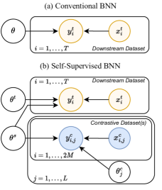
Figure 2: BNN Probabilistic Models (a) Probabilistic model for conventional BNNs. (b) Probabilistic model for self-supervised BNNs. We share parameters between different tasks, which allows us to condition on generated self-supervised data when making predictions on a new task. $j$ indexes self-supervised tasks, $i$ indexes datapoints.

$$p(y_{\star}^{t} |x_{\star},\{\mathcal{D}^{c}_{j}\}_{j=1}^{L},\mathcal{D}^{t})$$ (1)

$$=\mathbb{E}_{p(\theta^{s}|\{\mathcal{D}^{c}_{j}\}_{j=1}^{L},\mathcal{D}^{t})}[\mathbb{E}_{p(\theta^{t}|\theta^{s},\mathcal{D}^{t})}[p(y_{\star}^{t}|x_{\star},\theta^{s},\theta^{t})]],$$

where we have (i) noted that the downstream task parameters $\theta^{t}$ are independent of $\{\mathcal{D}^{c}_{j}\}_{j=1}^{L}$ given the shared parameters $\theta^{s}$ and (ii) integrated over each $\theta^{c}_{j}$ and $\theta^{t}$ in the definition of $p(\theta^{s}|\{\mathcal{D}^{c}_{j}\}_{j=1}^{L},\mathcal{D}^{t})$.

Alternatively, one can learn a point estimate for $\theta^{s}$, e.g., with MAP estimation, and perform full posterior inference for $\theta^{t}$ and $\theta^{c}_{j}$ only. This would be a partially stochastic network, which Sharma et al. (2022) showed often outperform fully stochastic networks while being more practical, and can also be justified as we can generate many contrastive tasks. This corresponds to model learning as used in deep kernels and variational autoencoders (Kingma and Welling, 2013; Wilson et al., 2015; Rezende and Mohamed, 2015; Wilson et al., 2016).

We now show these modifications incorporate information from $\mathcal{D}^{u}$ and the augmentations $\mathcal{A}$ into the downstream task prior predictive. Under the Bayesian approach, self-supervised BNNs push forward the posterior over $\theta^{t}$ and $p(\theta^{s}|\{\mathcal{D}^{c}_{j}\}_{j=1}^{L},\mathcal{D}^{t})\propto p(\theta^{s}|\{\mathcal{D}^{c}_{j}\}_{j=1}^{T})\,p(\mathcal{D}^{t}|\theta^{s})$ through the network to make predictions. In contrast, a standard BNN uses $p(\theta|\mathcal{D}^{t})\propto p(\theta)\,p(\mathcal{D}^{t}|\theta)$. We see that self-supervised BNNs use $\{\mathcal{D}^{c}_{j}\}_{j=1}^{L}$ to update the prior over the shared parameters $p(\theta^{s})$. Alternatively, if we learnt a point estimate for $\theta^{s}$ and used the Bayesian approach for $\theta^{t}$, this would define the prior predictive:

$$p(y_{\star}^{t} |x_{\star},\{\mathcal{D}^{c}_{j}\}_{j=1}^{L})=\mathbb{E}_{p(\theta^{t})}[p(y_{\star}^{t}|x_{\star},\theta^{s}_{\star},\theta^{t})],$$ (2)

where $\theta^{s}_{\star}$ is a point estimate for $\theta^{s}$ learnt using $\{\mathcal{D}^{c}_{j}\}_{j=1}^{L}$. Since the contrastive datasets were constructed to reflect our prior beliefs, both conditioning and training on them should be helpful.

3.2 Practical Self-Supervised Bayesian Neural Networks

We now use our framework to propose a practical two-step algorithm for self-supervised BNNs.

Preliminaries  We focus on image-classification problems. We use an encoder $f_{\theta^{s}}(\cdot)$ that maps images to representations and is shared across the contrastive tasks and the downstream task. The shared parameters $\theta^{s}$ thus are the base encoder’s parameters. We also normalise the representations produced by this encoder. For the downstream dataset, we use a linear readout layer from the encoder representations, i.e., we have $\theta^{t}=\{W^{t},b^{t}\}$ and $y^{t}_{i}\sim\operatorname{softmax}(W^{t}f_{\theta^{s}}(x_{i})+b^{t})$. The rows of $W^{t}_{j}$ are thus class template vectors. For the contrastive tasks, we use a linear layer without biases, i.e., $\theta^{c}_{j}=W^{c}_{j}$, and $j$ indexes contrastive tasks. We place Gaussian priors over $\theta^{s}$, $\theta^{t}$, and each $\theta^{c}_{j}$.

Pre-training $\theta^{s}$ (Step I)

Here, we learn a point estimate for the base encoder parameters $\theta^{s}$, which induces a prior predictive distribution over the downstream task labels (see Eq. 2). To learn $\theta^{s}$, we want to optimise the (potentially penalised) log-likelihood $\log p(\{\mathcal{D}^{c}_{j}\}_{j=1}^{L},\mathcal{D}^{t}|\theta^{s})$, but this would require integrating over $\theta^{t}$ and each $\theta^{c}$. Instead, we use the evidence lower bound (ELBO):

$$\tilde{\mathcal{L}}^{c}_{j}(\theta^{s})=\mathbb{E}_{q(\theta^{c}_{j})}[\log p(\mathcal{D}^{c}_{j}|\theta^{s},\theta^{c}_{j})]-D_{\text{KL}}(q(\theta^{c}_{j})||p(\theta^{c}_{j}))\leq\log p(\mathcal{D}^{c}_{j}|\theta^{s}),$$ (3)

where $q(\theta^{c}_{j})$ is a variational distribution over the contrastive task parameters. Rather than learning a different variational distribution for each contrastive task $j$, we amortise the inference and exploit the structure of the contrastive task. The contrastive task is to predict the source image index from pairs of augmented images using a linear layer from an encoder that produces normalised representations. We define $\omega_{i}=0.5(f_{\theta^{s}}(\tilde{x}_{i}^{A})+f_{\theta^{s}}(\tilde{x}_{i}^{B}))$, i.e., $\omega_{i}$ is the mean representation for each augmented pair of images, and because the rows of $W^{c}_{j}$ correspond to class templates, we thus use:

$$q(W^{c}_{j};\tau,\sigma^{2})=\mathcal{N}(\mu_{j}^{c},\sigma^{2}I),\text{with}\ \mu_{j}^{c}=\begin{bmatrix}\omega_{1}^{T}&\ldots&\omega_{M}^{T}\end{bmatrix}/\tau$$ (4)

In words, the mean representation of each augmented image pair is the class template for each source image, which should solve the contrastive task well. The variational parameters $\tau$ and $\sigma^{2}$ determine the magnitude of the linear layer and the per-parameter variance, are shared across contrastive tasks $j$, and are learnt by maximising Eq. 3 with reparameterisation gradients (Kingma and Welling, 2013).

Both the contrastive tasks and downstream task provide information about the base encoder parameters $\theta^{s}$. One option would be to learn the base encoder parameters $\theta^{s}$ using only data derived from $\mathcal{D}^{u}$ (Eq. 3), which would correspond to a standard self-supervised learning setup. In this case, the learnt prior would be task-agnostic. An alternative approach is to use both $\mathcal{D}^{t}$ and $\mathcal{D}^{u}$ to learn $\theta^{s}$, which corresponds to a semi-supervised setup. To do so, we can use the ELBO for the downstream data:

$$\tilde{\mathcal{L}}^{t}(\theta^{s})=\mathbb{E}_{q(\theta^{t})}[\log p(\mathcal{D}^{t}|\theta^{t},\theta^{s})]-D_{\text{KL}}[q(\theta^{t})||p(\theta^{t})]\leq\log p(\mathcal{D}^{t}|\theta^{s}),$$ (5)

where $q(\theta^{t})=\mathcal{N}(\theta^{t};\mu^{t},\Sigma^{t})$ is a variational distribution over the downstream task parameters; $\Sigma^{t}$ is diagonal. We can then maximise $\sum_{j}\tilde{\mathcal{L}}^{c}_{j}(\theta^{s})+\alpha\cdot\tilde{\mathcal{L}}^{t}(\theta^{s})$, where $\alpha$ is a hyper-parameter that controls the weighting between the downstream task and contrastive task datasets. We consider both variants of our approach, using Self-Supervised BNNs to refer to the variant that pre-trains only with $\{\mathcal{D}^{c}_{j}\}_{j=1}^{L}$ and Self-Supervised BNNs* to refer to the variant that uses both $\{\mathcal{D}^{c}_{j}\}_{j=1}^{L}$ and $\mathcal{D}^{t}$ .

Algorithm 1 Self-Supervised BNNs

Input: augmentations $\mathcal{A}$, unlabelled data $\mathcal{D}^{u}$, task data $\mathcal{D}^{t}$, contrastive prior $p(W^{c})$

for $j=1,\ldots,L$ do $\triangleright$ Unsupervised prior learning

     Draw subset $\{\hat{x}_{i}\}_{i=1}^{M}$, set $\mathcal{D}^{c}_{j}=\{\}$

     for $i=1,\ldots,M$ do $\triangleright$ Create contrastive task

         Sample $a^{A},a^{B}\sim\mathcal{A}$

         $\tilde{x}_{i}^{A}=a^{A}(\hat{x}_{i})$, $\tilde{x}_{i}^{B}=a^{B}(\hat{x}_{i})$

         $\tilde{z}_{i}^{A}=f_{\theta^{s}}(\tilde{x}_{i}^{A})$, $\tilde{z}_{i}^{B}=f_{\theta^{s}}(\tilde{x}_{i}^{B})$

         $\omega_{i}=0.5(\tilde{z}_{i}^{A}+\tilde{z}_{i}^{B})$

         Add $(\tilde{x}_{i}^{A},i)$ and $(\tilde{x}_{i}^{B},i)$ to $\mathcal{D}^{c}_{j}$.

     end for

     $W^{c}_{j}=\begin{bmatrix}\omega_{1}^{T}&\ldots&\omega_{M}^{T}\end{bmatrix}/\tau+\epsilon$,

      with $\epsilon\sim\mathcal{N}(0,\sigma^{2}I)$

     $\tilde{\mathcal{L}}(\tau,\sigma^{2},\theta^{s})=\log p(\theta^{s})+\frac{1}{2M}p(\mathcal{D}^{c}_{j}|\theta^{s},W_{j}^{c})$

      $-\bar{D}_{\text{KL}}[q(W_{j}^{c})||p(W^{c}))]$

     Update $\theta^{s},\tau,\sigma^{2}$ to maximise $\tilde{\mathcal{L}}(\tau,\sigma^{2},\theta^{s})$

end for

Approximate $p(\theta^{t}|\mathcal{D}^{t},\theta^{s})\simeq q(\theta^{t})$ $\triangleright$ Evaluation

Predict using $\mathbb{E}_{q(\theta^{t})}[p(y_{\star}^{t}|x_{\star},\theta^{s},\theta^{t})]$

Downstream Evaluation (Step II)

Having learnt a point estimate for $\theta^{s}$, we can use any approximate inference algorithm to infer $\theta^{t}$. Here, we use a post-hoc Laplace approximation (Mackay, 1992; Daxberger et al., 2021).

Algorithm 1 summarises Self-Supervised BNNs, which learn $\theta^{s}$ with $\mathcal{D}^{u}$ only. We found tempering with the mean-per-parameter KL divergence, $\bar{D}_{\text{KL}}$, improved performance, in line with other work (e.g., Krishnan et al., 2022). Moreover, we generate a new $\mathcal{D}^{c}_{j}$ per gradient step so $L$ corresponds to the number of gradient steps. We also regularise with $\log p(\theta^{s})$, which here corresponds to weight decay. Finally, following best-practice for contrastive learning (Chen et al., 2020a), we use a non-linear projection head $g_{\psi}(\cdot)$ only for the contrastive tasks. For further details, see Appendix A.

Understanding the Approximate Posterior

To better understand $q(W_{j}^{c};\tau,\sigma^{2})$ (Eq. 4), we evaluate the likelihood term of Eq. 3 at the approximate posterior’s mean: $\mu_{j}^{c}$. Define $\tilde{z}_{i}^{A}=f_{\theta^{s}}(\tilde{x}_{i}^{A})$ and $\tilde{z}_{i}^{B}=f_{\theta^{s}}(\tilde{x}_{i}^{B})$, and recall we have $\omega_{i}=0.5(\tilde{z}_{i}^{A}+\tilde{z}_{i}^{B})$. Then:

$$\log p(\mathcal{D}^{c}_{j}|\theta^{s},\mu_{j}^{c})=\sum_{i=1}^{M}\Big{[}\log\frac{\exp\omega_{i}^{T}\tilde{z}_{i}^{A}/\tau}{\sum_{j=1}^{M}\exp\omega_{j}^{T}\tilde{z}_{i}^{A}/\tau}+\log\frac{\exp\omega_{i}^{T}\tilde{z}_{i}^{B}/\tau}{\sum_{j=1}^{M}\exp\omega_{j}^{T}\tilde{z}_{i}^{B}/\tau}\Big{]},$$ (6)

which we see takes the form of a (negative) normalised-temperature cross-entropy loss (NT-XENT), as used in contrastive learning algorithms like SimCLR (Chen et al., 2020b). However, there are some differences between these objectives. In terms of learning the base-encoder parameters, our objective: (i) is a principled lower bound for the log-marginal likelihood, $\log p(\mathcal{D}^{c}_{j}|\theta^{s})$; (ii) injects noise around $\mu_{j}^{c}$, which may be a helpful regularisation (Srivastava et al., 2014); and (iii) adapts the temperature $\tau$ throughout training, which may be beneficial (Huang et al., 2022).

Pre-training as Prior Learning

Since our objective function is a principled lower bound on the log-marginal likelihood, it is similar to type-II maximum likelihood (ML), which is often used to learn parameters for deep kernels (Wilson et al., 2015) of Gaussian processes (Williams and Rasmussen, 2006), and recently also for BNNs (Immer et al., 2021). As such, similar to type-II ML, our approach can be understood as a form of prior learning. Although we learn only a point-estimate for $\theta^{s}$, this fixed value induces a prior distribution over predictive functions through the task-specific prior $p(\theta^{t})$. However, while normal type-II ML learns this prior using the observed data itself, our approach maximises a marginal likelihood derived from unsupervised data. Because we maximise an ELBO during pre-training, our approach can similarly be understood as variational model learning.

4 How Good Are Self-Supervised BNN Prior Predictives?

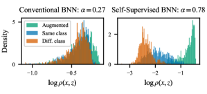
Figure 3: BNN Prior Predictives. We investigate prior predictives by computing the probability $\rho$ that particular image pairs have the same label under the prior, and examining the distribution of $\rho$ across different sets of image pairs. We consider three sets of differing semantic similarity: (i) augmented images; (ii) images of the same class; and (iii) images of different classes. Left: Conventional BNN prior. Right: Self-supervised BNN learnt prior predictive. The self-supervised learnt prior reflects the semantic similarity of the different image pairs better than the BNN prior, which is reflected in the prior evaluation score, $\alpha$.

We showed our approach incorporates unlabelled data into the downstream task prior predictive distribution (Eq. 2). We also argued that as the generated contrastive data reflect our subjective beliefs about the semantic similarity of different image pairs, incorporating the unlabelled data should improve the prior predictive. We now examine whether this is indeed the case.

However, although prior predictive checks are standard in the applied statistics community (Gelman et al., 1995), they are challenging to apply to BNNs due to the high dimensionality of the input space. To proceed, we note, intuitively, a suitable prior should reflect a belief that the higher the semantic similarity between pairs of inputs, the more likely these inputs are to have the same label. Therefore, rather than inspecting the prior predictive at single points in input space, we examine the joint prior predictive of pairs of inputs with known semantic relationships. Indeed, it is far easier to reason about the relationship between examples than to reason about distributions over high-dimensional functions.

Here, we focus on image classification and consider the following pairs of images: (i) an image from the validation set (the “base image”) and an augmented version of the same image; (ii) a base image and another image of the same class; and (iii) a base image and an image of a different class. As these image pair groups have decreasing semantic similarity, we want the first group to be the most likely to have the same label, and the last group to be the least likely.

Experiment Details

We investigate the different priors on CIFAR10. For the BNN, we follow Izmailov et al. (2021b) and use a ResNet-20-FRN with a $\mathcal{N}(0,1/5)$ prior over the parameters. For the self-supervised BNN, we learn a base encoder of the same architecture with $\mathcal{D}^{u}$ only and sample from the task prior predictive using Eq. 2. $\theta^{t}$ are the parameters of the linear readout layer. We also pre-train a base encoder with SimCLR. For further details, see Section C.3.

Table 1: Prior Evaluation Scores. Mean and standard deviation across three seeds shown. Self-supervised priors are better than standard BNN priors.

Prior Predictive	Prior Score $\alpha$
BNN — Gaussian	0.261 $\pm$ 0.024
BNN — Laplace	0.269 $\pm$ 0.007
SimCLR	0.670 $\pm$ 0.015
Self-Supervised BNN	0.680 $\pm$ 0.063

Graphical Evaluation

First, we visualise the BNN and self-supervised BNN prior predictive (Fig. 1 and 3). The BNN prior predictive reflects a belief that all three image pair groups are similarly likely to have the same label, and thus does not capture semantic information well. In contrast, the self-supervised prior reflects a belief that image pairs with higher semantic similarity are more likely to have the same label. In particular, the self-supervised prior is able to distinguish between image pairs of the same class and of different classes, even without access to any ground-truth labels.

Quantitative Evaluation

We now quantify how well different prior predictives reflect data semantics. We define $\rho(x,z)$ as the probability that inputs $x,z$ have the same label under the prior predictive, i.e., $\rho(x,z)=\mathbb{E}_{\theta}[p(y(x)=y(z)|\theta)]$ where $y(x)$ is the label corresponding to input $x$. We want a prior where image pairs with higher semantic similarity have higher values of $\rho$. Therefore, to quantify the suitability of the prior predictive, we evaluate the frequency $\alpha$ under the data distribution that the ranking of $\rho$s that correspond to the aforementioned three sets of image pairs indeed match the ranking of semantic similarities. Mathematically, we have $\alpha=\mathbb{E}_{x,z_{1:3}}[\mathbb{I}({\color[rgb]{0.0078,0.6196,0.450980}\rho(x,z_{1})}>{\color[rgb]{0.0039,0.45098,0.98039}\rho(x,z_{2})}>{\color[rgb]{0.7,0.44,0}\rho(x,z_{3})})]$, where each of the $\rho$-terms above corresponds to a different image pair group: ${\color[rgb]{0.0078,0.6196,0.450980}\rho(x,z_{1})}$ corresponds to augmented image pairs, ${\color[rgb]{0.0039,0.45098,0.98039}\rho(x,z_{2})}$ to same-class image pairs, and $\color[rgb]{0.7,0.44,0}\rho(x,z_{3})$ to different-class image pairs. $\alpha$ is therefore a generalisation of the AUROC metric.

In Table 1, we see that conventional BNN priors reflect semantic similarity much less than self-supervised BNN priors. Further, SimCLR, a contrastive learning approach, also induces a prior predictive that well reflects semantic similarity well if the trained encoder is combined with a stochastic last-layer, which may underpin its success.

5 Experiments

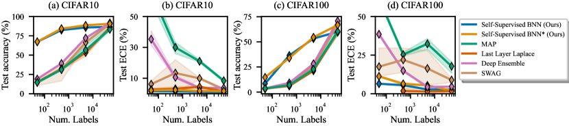
Figure 4: BNN Label Efficiency. We compute the test accuracy and expected calibration error (ECE) when observing different numbers of labels. Self-Supervised BNNs pre-train the base-encoder parameters using $\mathcal{D}^{u}$ only, while Self-Supervised BNNs* also use $\mathcal{D}^{t}$. Mean and standard deviation across 3 seeds shown. Self-supervised BNNs substantially outperform conventional BNNs at most dataset sizes, highlighting the benefit of incorporating unlabelled data into the BNN framework.

We saw that self-supervised BNN prior predictives reflect semantic similarity better than conventional BNNs (§3). We now investigate whether this translates to improved predictions in semi-supervised and active learning setups, which mimic scenarios where there is an abundance of unlabelled data, but labelling data points is expensive. We find that our approach combines the label efficiency of self-supervised methods and the uncertainty estimates of Bayesian approaches.

5.1 Semi-Supervised Learning

Experiment Details We consider CIFAR10 and CIFAR100, reserving a validation set of 1000 examples from the test set and using the remaining 9000 examples as the test set. We evaluate the performance of different baselines when conditioning on 50, 500, 5000, and 50000 labels. All baselines use a ResNet-18 modified for CIFAR image size. For self-supervised BNNs, we use a non-linear projection head for pre-training, as standard, and use the full train set for pre-training with the data augmentations suggested by Chen et al. (2020a). We consider two variants of self-supervised BNNs: Self-Supervised BNNs learn the base-encoder parameters using $\mathcal{D}^{u}$ only, while Self-Supervised BNNs* also utilise $\mathcal{D}^{t}$. For evaluation, we use a post-hoc Laplace approximation on the last-layer. For the conventional BNN baselines, we use MAP, SWAG (Maddox et al., 2019), a deep ensemble (Lakshminarayanan et al., 2017), and last-layer Laplace (Daxberger et al., 2021). We include standard data augmentation for the baselines, which were chosen because they support batch normalisation (Ioffe and Szegedy, 2015). We also compare to SimCLR, where we consider both the standard linear-evaluation protocol (i.e., maximum likelihood) as well as a post-hoc Laplace approximation on the last-layer. See Appendix C for further details.

Fig. 4 shows the performance of different BNNs in terms of test accuracy and expected calibration error. Self-supervised BNNs substantially outperform conventional BNNs at all but the largest data set size, a finding in line with our results that self-supervised BNN prior predictives are better than conventional BNN priors (§3). We also find self-supervised BNNs provide well-calibrated uncertainty estimates at all dataset sizes, and that incorporating labelled data when learning the base encoder improves accuracy. Indeed, at the largest dataset size, Self-Supervised BNNs*, which leverage the labelled examples as well as unlabelled data to learn the base encoder parameters, are competitive in terms of accuracy and calibration with the deep ensemble, which is the strongest baseline but uses five trained networks. These results highlight the benefit of incorporating unlabelled data into BNNs.

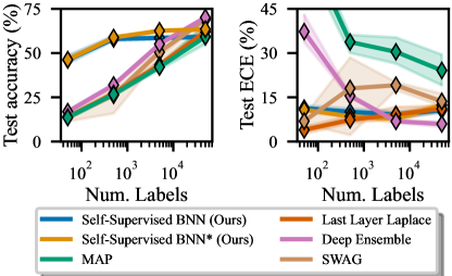
Figure 5: Out-of-Distribution Generalisation. We train BNNs on the standard CIFAR10 dataset and evaluate on CIFAR-10-C with corruption intensity 5 (Hendrycks and Dietterich, 2019). Results averaged across corruptions, mean and std. across 3 seeds shown. Self-Supervised BNNs pre-train the base-encoder parameters using $\mathcal{D}^{u}$ only, while Self-Supervised BNNs* also use $\mathcal{D}^{t}$. Self-supervised BNNs outperform conventional BNNs at most dataset sizes.

Further, we evaluate the out-of-distribution generalisation performance of different BNNs. To do so, we condition BNNs on different numbers of labels of CIFAR10 as before, but evaluate the test accuracy and calibration on the CIFAR-10-C dataset (Hendrycks and Dietterich, 2019), following Ovadia et al. (2019). Again, self-supervised BNNs can benefit from unlabelled training examples, while conventional BNNs are unable to do so.

In Fig. 5, we see that self-supervised BNNs not only outperform conventional BNNs at most dataset sizes in terms of accuracy, but they consistently offer well-calibrated uncertainty estimates. On the largest dataset size, self-supervised BNNs are outperformed by SWAG and deep ensembles, which are strong baselines but use several trained networks. However, deep ensembles are poorly calibrated at small dataset sizes. These results provide further evidence for the benefits of incorporating unlabelled data into BNNs.

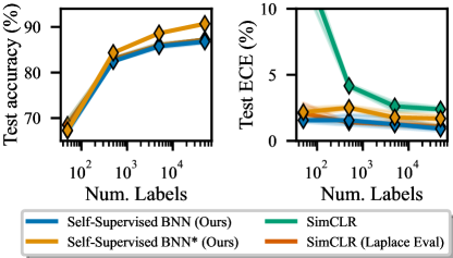
Figure 6: Comparison to SimCLR on CIFAR10. We compare self-supervised BNNs with (i) standard SimCLR, and (ii) SimCLR with a post-hoc Laplace approximation over the last-layer. Self-Supervised BNNs pre-train the base-encoder parameters using $\mathcal{D}^{u}$ only, while Self-Supervised BNNs* also utilise $\mathcal{D}^{t}$ during pre-training. Approximate inference over the task-specific parameters improves calibration, while pre-training with both $\mathcal{D}^{t}$ and $\mathcal{D}^{u}$ improves accuracy.

We now compare our approach with standard SimCLR on CIFAR10. Recall that, relative to SimCLR, our approach uses a modified pre-training objective that is a lower bound on a marginal likelihood and performs approximate inference over $\theta^{t}$ when making predictions. We also consider combining SimCLR with approximate inference for the last-layer parameters to disentangle the effects of the pre-training objective and evaluation protocol.

In Fig. 6, Self-Supervised BNNs match SimCLR in terms of accuracy, while offering better-calibrated uncertainty estimates. All approaches have high accuracy at low data regimes, highlighting the benefit of leveraging unlabelled data. We find that incorporating $\mathcal{D}^{t}$ when learning the base-encoder (Self-Supervised BNNs*) substantially improves accuracy, though surprisingly, it slightly hurts calibration. In contrast, the Laplace evaluation protocol improves calibration, and indeed, SimCLR combined with approximate inference is a strong baseline. This matches our previous observation that SimCLR pre-training and a prior over $\theta^{t}$ induce a prior predictive that well captures image semantics (§3).

5.2 Active Learning

Experiment Details

We consider low-budget active learning, which simulates a scenario where labelling examples is extremely expensive. We use the CIFAR10 training set as the unlabelled pool set from which to label points. We assume an initial train set of 50 labelled points, randomly selected, and a validation set of the same size. We acquire 10 labels per acquisition round up to 500 labels and evaluate using the full test set. We compare self-supervised BNNs, SimCLR, and a deep ensemble. We use BALD (Houlsby et al., 2011) as the acquisition function for the deep ensemble and self-supervised BNN, because they provide epistemic uncertainty estimates, while we use predictive entropy for SimCLR. We also consider uniform selection. See Appendix C for more details.

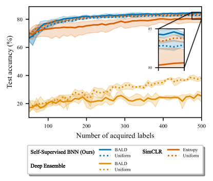
Figure 7: Low-Budget Active Learning on CIFAR10. We compare: (i) a self-supervised BNN; (ii) SimCLR; and (iii) a deep ensemble. For the self-supervised BNN and the ensemble, we acquire points with BALD; predictive entropy for SimCLR. We also use uniform sampling for all methods. Mean and std. shown (3 seeds). The methods that incorporate unlabelled data perform best, and self-supervised BNNs are the only method where active learning outperforms uniform sampling.

In Fig. 7, we see that the methods that leverage unlabelled data perform the best. In particular, the self-supervised BNN with BALD selection achieves the highest accuracy across most numbers of labels, and is the only method for which active learning improves performance. Surprisingly, uniform selection is a strong baseline.

6 Related Work

Improving BNN Priors  We demonstrated that BNNs have poor prior predictive distributions (§3), a concern shared by others (e.g., Wenzel et al., 2020; Noci et al., 2021; Izmailov et al., 2021a). The most common approaches to remedy this are through designing better priors, typically over network parameters (Louizos et al., 2017; Nalisnick, 2018; Atanov et al., 2019; Fortuin et al., 2021b) or predictive functions directly (Sun et al., 2019; Tran et al., 2020; Matsubara et al., 2021, see Fortuin (2022) for an overview). In contrast, our approach incorporates vast stores of unlabelled data into the prior predictive distribution through variational model learning. Similarly, other work also learns priors, but typically using labelled data e.g., by using meta-learning (Garnelo et al., 2018; Rothfuss et al., 2021) or type-II maximum likelihood (Wilson et al., 2015; Immer et al., 2021). Finally, Shwartz-Ziv et al. (2022) use generic transfer learning, potentially from an unsupervised task, for better BNN priors. While they consider fully stochastic networks, we use partially stochastic networks with a pre-training objective that is a principled lower bound on a log-marginal likelihood derived from unlabelled data. A further difference is that our work incorporates pre-training within the probabilistic modelling framework itself.

Understanding Contrastive Learning  Our work shows that contrastive pre-training induces a prior predictive distribution that captures semantic similarity well (§3), and further offers a Bayesian interpretation of contrastive learning (§3). There has been much other work on understanding contrastive learning (e.g., Wang and Isola, 2020; Wang and Liu, 2021). Some work appeals to the InfoMax principle (Becker and Hinton, 1992), which maximises the mutual information between representations of two views of an input datum, while our framework operates in predictive space. Zimmermann et al. (2022) argue that contrastive learning inverts the data-generating process, while Aitchison (2021) cast InfoNCE as the objective of a self-supervised variational auto-encoder.

Semi-Supervised Deep Generative Models  Deep generative models (DGMs) are an alternative approach for label-efficient learning (Kingma and Welling, 2013; Kingma et al., 2014; Joy et al., 2020). DGMs generate supervision by reconstructing data through compact representations, i.e., they are generative. Our framework, however, is discriminative—supervision works through pseudo-labelled tasks. Ganev and Aitchison (2021) formulate several semi-supervised learning objectives as lower bounds of log-likelihoods in a probabilistic model of data curation. Finally, Sansone and Manhaeve (2022) unify self-supervised learning and generative modelling under one framework.

7 Conclusion

We introduced Self-Supervised Bayesian Neural Networks, which leverage unlabelled data for improved prior predictive distributions (§3). We showed that self-supervised BNNs, as well as other self-supervised methods, learn prior predictives that reflect semantics of the data (§3). In our experiments, self-supervised BNNs combine the label-efficiency of self-supervised methods and the uncertainty estimates of Bayesian approaches (§4), and thus are a principled, practical, and performant alternative to conventional BNNs. We strongly encourage practitioners to incorporate unlabelled data into their Bayesian Neural Networks through unsupervised prior learning.

Acknowledgements

MS was supported by the EPSRC Centre for Doctoral Training in Autonomous Intelligent Machines and Systems (EP/S024050/1), and thanks Rob Burbea for inspiration and support. VF was supported by a Postdoc Mobility Fellowship from the Swiss National Science Foundation, a Research Fellowship from St John’s College Cambridge, and a Branco Weiss Fellowship.

Appendix A Self-Supervised BNNs: Further Considerations

We introduced Self-Supervised BNNs (§3), which benefit from unlabelled data for improved predictive performance within the probabilistic modelling framework. To summarise, our conceptual framework uses data augmentation to create a set of contrastive datasets $\{\mathcal{D}^{c}_{j}\}_{j=1}^{L}$. In our probabilistic model, conditioning on this data is equivalent to incorporating unlabelled data into the task prior predictive. We now discuss further considerations and provide further details.

Theoretical Considerations

In §3.1, we treated the number of contrastive task datasets, $L$, as a fixed hyper-parameter. However, one could generate an potentially infinite number of datasets, in which case, the posterior $p(\theta^{s}|\{\mathcal{D}^{c}_{j}\}_{j=1}^{L},\mathcal{D}^{t})\propto p(\theta^{s})\cdot p(\mathcal{D}^{t}|\theta^{s})\cdot\prod_{j=1}^{L}p(\mathcal{D}^{c}_{j}|\theta^{s})$ will collapse to a delta function, and will be dominated by the contrastive tasks. This justified learning a point estimate for $\theta^{s}$, but if one wanted to avoid this behaviour, they could re-define the posterior:

$$\tilde{p}(\theta^{s}|\{\mathcal{D}^{c}_{j}\}_{j=1}^{L},\mathcal{D}^{t})\propto p(\theta^{s})\cdot p(\mathcal{D}^{t}|\theta^{s})\cdot\prod_{j=1}^{L}p(\mathcal{D}^{c}_{j}|\theta^{s})^{\gamma/L}.$$ (7)

The log-posterior would equal, up to a constant:

$$\log\tilde{p}(\theta^{s}|\{\mathcal{D}^{c}_{j}\}_{j=1}^{L},\mathcal{D}^{t})=\log p(\theta^{s})+\log p(\mathcal{D}^{t}|\theta^{s})+\frac{\gamma}{L}\sum_{j=1}^{L}\log p(\mathcal{D}^{c}_{j}|\theta^{s}).$$ (8)

Here, the total evidence contributed by the contrastive datasets is independent of $L$, and instead controlled by the hyper-parameter $\gamma$. This is equivalent to posterior tempering. The final term of the above equation could also be re-defined as an average log-likelihood when sampling different $\mathcal{D}^{c}$. i.e., we could use:

$$\log\tilde{p}(\theta^{s}|\mathcal{D}^{u},\mathcal{D}^{t})=\log p(\theta^{s})+\log p(\mathcal{D}^{t}|\theta^{s})+\gamma\mathbb{E}_{\mathcal{D}^{c}}[p(\mathcal{D}^{c}|\theta^{s})].$$ (9)

In this case, we look for a distribution over $\theta^{s}$ where $\mathcal{D}^{c}$ has high-likelihood on average. Our practical algorithm samples a different $\mathcal{D}^{c}$ per gradient-step, and instead weights the $\mathcal{D}^{t}$ term with $\alpha$, which is similar to the above approach if we set $\alpha=1/\gamma$ and modify the prior term as needed. Re-defining the framework in this way allows it to support potentially infinite numbers of generated contrastive datasets. We further note that this framework could naturally be extended to multi-task scenarios.

Practical Considerations

In practice, we share parameters $\theta^{s}$ across all tasks (i.e., across the generated contrastive tasks and the actual downstream task), and learn a $\theta^{t}$ separately for each task. We focus on image classification problems and let $\theta^{s}$ be the parameters of a base encoder, which produces a representation $z$. $\theta^{t}$ are the parameters of a linear readout layer that makes predictions from $z$. We discussed learning a point-estimate for $\theta^{s}$ by optimising an ELBO derived from the unlabelled data only:

$$\tilde{\mathcal{L}}^{c}_{j}(\theta^{s})=\mathbb{E}_{q(\theta^{c}_{j})}[\log p(\mathcal{D}^{c}_{j}|\theta^{s},\theta^{c}_{j})]-D_{\text{KL}}(q(\theta^{c}_{j})||p(\theta^{c}_{j}))\leq\log p(\mathcal{D}^{c}_{j}|\theta^{s}).$$ (10)

We (optionally) further include an ELBO dervied using task-specific data:

$$\tilde{\mathcal{L}}^{t}(\theta^{s})=\mathbb{E}_{q(\theta^{t})}[\log p(\mathcal{D}^{t}|\theta^{t},\theta^{s})]-D_{\text{KL}}[q(\theta^{t})||p(\theta^{t})]\leq\log p(\mathcal{D}^{t}|\theta^{s}).$$ (11)

Our final objective is:

$$\mathcal{L}(\theta^{s})=\log p(\theta^{s})+\alpha\tilde{\mathcal{L}}^{t}(\theta^{s})+\mathbb{E}_{\mathcal{D}^{c}}[\tilde{\mathcal{L}}^{c}_{j}],$$ (12)

where $\alpha=0$ would learn the base-encoder parameters only using the unlabelled data. $\alpha$ controls the weighting between the generated contrastive task data and the downstream data. We see the above objective is closely related to a (lower bound of) Eq. 9. We further modify this objective function because they follow best-practice, either in the contrastive learning or Bayesian deep learning communities, and improve performance.

1. We add a non-linear projection head to the base encoder architecture only for the contrastive task datasets. As such, we use $z=g_{\phi}(f_{\theta^{s}}(x))/||g_{\phi}(f_{\theta^{s}}(x))||$ for $\mathcal{D}^{c}$. $g_{\phi}(\cdot)$ is the projection head, and the representation is normalised. For the downstream tasks, we use $z=f_{\theta^{s}}(x)$, i.e., we “throw-away” the projection head. This is best practice within the contrastive learning community (Chen et al., 2020a, b).

2. We temper the KL divergence term, using the mean-per-parameter KL divergence (denoted as $\bar{D}_{\text{KL}}(\cdot||\cdot)$). Tempering is necessary for several Bayesian deep learning algorithms to perform well (Wenzel et al., 2020; Krishnan et al., 2022).

3. We generate a new contrastive task dataset per gradient step, update on that dataset, and then discard it. This follows standard contrastive learning algorithms (Chen et al., 2020a).

4. We rescale the likelihood terms in the ELBOs $\tilde{\mathcal{L}}^{t}(\theta^{s})$ and $\tilde{\mathcal{L}}^{c}_{j}(\theta^{s})$ to be average per-datapoint log-likelihoods. e.g., we use $1/{|\mathcal{D}^{c}_{j}|}\log p(\mathcal{D}^{c}_{j}|\theta^{t}_{j},\theta^{s})$.

5. Instead of having an explicit prior distribution over $\theta^{s}$, we use standard weight-decay for training i.e., we specify a penalty on the norm of the weights of the encoder per gradient step.

Together, these changes yield the objective function used in Algorithm 1. Finally, we note that different practical algorithms ensue depending on the choice of $\theta^{t}$, the choice of $\theta^{s}$, and the techniques used to perform approximate inference. We employ variational inference and learn a point estimate for $\theta^{s}$, but there are other choices possible.

Appendix B Ethical Considerations

We hope that incorporating unlabelled data into Bayesian Neural Networks will help pave the way for high-quality uncertainty estimates, particularly at low-data regimes. Though such uncertainty estimates would be useful, if unwarranted trust is placed in them, this could have unintended, potentially harmful consequences.

Appendix C Experiment Details

We now provide further experiment details and additional results. The vast majority of experiments were run on an internal compute cluster using Tesla V100 or Nvidia A100 GPUs. The maximum runtime for an experiment was less than 12 hours.

C.1 Semi-Supervised Learning (§4)

C.1.1 Datasets

We consider the CIFAR10 and CIFAR100 datasets (Krizhevsky et al., 2009). The entire training set is the unsupervised set, and we suppose that we have access to different numbers of labels. For the evaluation protocols, we reserve a validation set of 1000 data points from the test set and evaluate using the remaining 9000 labels.

To assess out-of-distribution generalisation, we further evaluation on the CIFAR-10-C dataset (Hendrycks and Dietterich, 2018). We compute the average performance across all corruptions with intensity level five.

C.1.2 Self-Supervised BNNs

Base Architecture

We use a ResNet-18 architecture, modified for the size of CIFAR10 images, following Chen et al. (2020a). The representations produced by this architecture have dimensionality $512$. Further, for the non-linear projection head, we use a 2 layer multi-layer perceptron (MLP) with output dimensionality 128.

Contrastive Augmentations

We follow Chen et al. (2020a) and compose a random resized crop, a random horizontal flip, random colour jitter, and random grayscale for the augmentation. These augmentations make up the contrastive augmentation set $\mathcal{A}$. We finally normalise the images to have mean 0 and standard deviation 1 per channel, as is standard.

Hyperparameters

We use a $\mathcal{N}(0,\frac{1}{\tau_{p}^{2}})$ prior over the linear parameters $\theta^{t}$, and tune $\tau_{p}$ for each dataset. As such, $\tau$ can be understood as the prior temperature. We use $\tau_{p}=0.65$ for CIFAR10 and $\tau_{p}=0.6$ for CIFAR100. We use weight decay $1e-6$ for the base encoder and projection head parameters.

Variational Distribution

We parameterize the temperature and noise scale using the $\log$ of their values. That is, we have $\sigma=\exp\tilde{\sigma}$.

Optimisation Details

We use the LARS optimiser (You et al., 2017), with batch size $1000$ and momentum $0.9$. We train for 500 epochs, using a linear warmup cosine annealing learning rate schedule. The warmup starting learning rate for the base encoder parameters is $1e-3$ with a maximum learning rate of $0.6$. For the variational parameters, the maximum learning rate is $1e-3$, which we found to be important for the stability of the algorithm.

Laplace Evaluation Protocol

We find a point estimate for $\theta^{t}$ found using the standard linear evaluation protocol (i.e., SGD training). We apply then post-hoc Laplace approximation using the generalised Gauss-Newton approximation to the Hessian using the Laplace library (Daxberger et al., 2021). For CIFAR10, we use a full covariance approximation and for CIFAR100 we use a Kroenker-factorised approximation for the Hessian of the last layer weights and biases. We tune the prior precision by maximising the likelihood of a validation set. For predictions, we use the (extended) probit approximation. These choices follow recommendations from Daxberger et al. (2021).

C.1.3 Self-Supervised BNNs*

Self-Supervised BNNs* additionally leverage labelled data when training the base encoder by including an additional ELBO $\tilde{\mathcal{L}}^{t}$ that depends on $\mathcal{D}^{t}$.

We use mean-field variational inference over $\theta^{t}$ with a Gaussian approximate posterior and Flipout (Wen et al., 2018). We use the implementation from Krishnan et al. (2022), and temper by setting $\beta=1/|\theta^{t}|$, meaning we use the average per-parameter KL divergence. $\alpha$ is a hyperparameter that controls the relative weighting between the generated contrastive task datasets and the observed label data, and is tuned. We use $\alpha=5\cdot 10^{-5}$ when we have fewer than 100 labels, and $\alpha=5\cdot 10^{-3}$ otherwise. For $p(\theta^{t})$, we use a $\mathcal{N}(0,1)$ prior. For downstream evaluation, we use the Laplace evaluation protocol.

All other details follow Self-Supervised BNNs.

C.1.4 BNN Baselines

All baselines use the same ResNet-18 architecture, which was modified for the image size used in the CIFAR image datasets. The baselines we considered were chosen because they are all compatible with batch normalisation, which is included in the base architecture. We provide further details about the baselines below.

MAP

For the maximum-a-posterior network, we use the Adam optimiser with learning rate $10^{-3}$, default weight decay, and batch size 1000. We train for a minimum of 25 epochs and a maximum of 300 epochs, terminating training early if the validation loss increases for 3 epochs in a row.

Last-Layer Laplace

For the Last-Layer Laplace baseline, we perform a post-hoc Laplace approximation to a MAP network trained using the protocol above. We use the same settings as for the self-supervised BNN’s Laplace evaluation..

Deep Ensemble

For the deep ensemble baseline, we train 5 MAP networks starting from different initialisations using the above protocol, and aggregate their predictions.

SWAG

For the SWAG baseline, we first a MAP network using the above protocol. We then run SGD from this solution for 10 epochs, taking 4 snapshots per epoch, and using $K=20$ as the rank of the covariance matrix. We choose the SWAG learning rate per run using the validation set, and consider $10^{-2},10^{-3}$, and $10^{-4}$.

C.1.5 SimCLR

SimCLR

For SimCLR (Chen et al., 2020a), we use the same hyperparameters as for the self-supervised BNNs, except that we separately tune the temperature parameter. We use $\tau=0.45$ for CIFAR10 and $\tau=0.3$ for CIFAR100, selected by maximising the average log-likelihood across multiple data sizes. For evaluation, we use the linear evaluation protocol.

Linear Evaluation Protocol

We update the last-layer linear readout parameters using the AdamW (Loshchilov and Hutter, 2017) optimiser with batch size 1000, no weight decay and learning rate $10^{-2}$. We train for a maximum of 300 epochs, but terminate training if the validation loss has not improved for 10 epochs. We use the checkpoint with the highest validation accuracy. We additionally use random resized crops and random horizontal flips as data augmentation that boosts the performance of the linear evaluation.

C.2 Active Learning (§4)

We simulate a low-budget active learning setting. For each method, we use their default implementation details as outlined in this Appendix. With regards to the active learning setup, we assume that we have access to a small validation set of $50$ labelled examples and are provided $50$ labelled training examples. We acquire $10$ examples per acquisition round up to a maximum of $500$ labelled examples, which corresponds to 1% of the labels in the training set. We evaluate using the full test set. For all methods (the deep ensemble, SimCLR, and self-supervised BNNs), we consider uniform sampling. The deep ensemble and self-supervised BNNs provide epistemic uncertainty estimates, so we perform active learning by selecting the points with the highest BALD metric (Houlsby et al., 2011). For SimCLR, we acquire points using the highest predictive entropy, a commonly used baseline (Gal et al., 2017). For this experiment, we use only the CIFAR10 dataset.

C.3 Prior Predictive Checks (§3)

BNN Prior Predictive

We use the ResNet-20-FRN architecture, which is the architecture used by Izmailov et al. (2021b). Note that this architecture does not include batch normalisation, which means the prior over parameters straightforwardly corresponds to a prior predictive distribution. We use a $\mathcal{N}(0,\frac{1}{5})$ prior over all network weights, again following Izmailov et al. (2021b), and sample from the prior predictive using 8192 Monte Carlo samples.

Self-Supervised Prior Predictives

We primarily follow the details outlined earlier , except we use the same ResNet-20-FRN architecture as used for the BNNs and batch size of 500 rather than 1000. To sample from the prior predictive, we use Eq. 2 and have $y\sim\operatorname{softmax}(Wf_{\theta^{s}}(x))$, where we normalise the representations produced by the base encoder to have zero mean and unit variance, and we have $W\sim\mathcal{N}(0,20)$, with the prior precision chosen by hand. We neglect the biases because they introduce additional variance. The prior evaluation scores are not sensitive to the prior variance choice, and are evaluated by sampling images from the validation set, which was not seen during training. We used $4096$ Monte Carlo samples from the prior.

Appendix D Ablation Studies

Effect of Batch Size

We study the effect of the pre-training batch size on the performance of our self-supervised BNNs. We run one seed for 100 epochs across three different batch sizes on CIFAR10. We see in Table 2, the performance on CIFAR10 is robust to reducing the batch size. We hypothesise this is due to the noise injected during pre-training.

Table 2: Effect of pretraining batch size on self-supervised BNN.

Batch Size	CIFAR10 Accuracy $(\%)$
100	0.81
500	0.81
1000	0.80

Effect of Variational Distribution

We run an ablation study changing the variational distribution mean on CIFAR10. We evaluation using one seed, training for 100 epochs only. We consider setting the mean of the variational distribution for image $i$, $\omega_{i}$, to be: $0.5(\tilde{z}_{i}^{A}+\tilde{z}_{i}^{B})$, $\tilde{z}_{i}^{A}$, and $\mathbf{0}$. We see a suitable mean is required for good performance.

Table 3: Effect of pretraining variational distribution mean on self-supervised BNN performance on CIFAR10.

Variational Dist. Mean	CIFAR10 Accuracy $(\%)$
$\mathbf{0}$	0.19
$\tilde{z}_{i}^{A}$	0.79
$0.5(\tilde{z}_{i}^{A}+\tilde{z}_{i}^{B})$	0.80

References

- Abdar et al. (2021) Moloud Abdar, Farhad Pourpanah, Sadiq Hussain, Dana Rezazadegan, Li Liu, Mohammad Ghavamzadeh, Paul Fieguth, Xiaochun Cao, Abbas Khosravi, U Rajendra Acharya, et al. A review of uncertainty quantification in deep learning: Techniques, applications and challenges. Information Fusion, 76:243–297, 2021.
- Aitchison (2021) Laurence Aitchison. InfoNCE is a variational autoencoder, July 2021. URL http://arxiv.org/abs/2107.02495. arXiv:2107.02495 [cs, stat].
- Atanov et al. (2019) Andrei Atanov, Arsenii Ashukha, Kirill Struminsky, Dmitry Vetrov, and Max Welling. The Deep Weight Prior. arXiv:1810.06943 [cs, stat], February 2019. URL http://arxiv.org/abs/1810.06943. arXiv: 1810.06943.
- Becker and Hinton (1992) Suzanna Becker and Geoffrey E. Hinton. Self-organizing neural network that discovers surfaces in random-dot stereograms. Nature, 355(6356):161–163, January 1992. ISSN 1476-4687. doi: 10.1038/355161a0. URL https://www.nature.com/articles/355161a0. Number: 6356 Publisher: Nature Publishing Group.
- Chen et al. (2020a) Ting Chen, Simon Kornblith, Mohammad Norouzi, and Geoffrey Hinton. A Simple Framework for Contrastive Learning of Visual Representations. arXiv:2002.05709 [cs, stat], June 2020a. URL http://arxiv.org/abs/2002.05709. arXiv: 2002.05709.
- Chen et al. (2020b) Ting Chen, Simon Kornblith, Kevin Swersky, Mohammad Norouzi, and Geoffrey Hinton. Big Self-Supervised Models are Strong Semi-Supervised Learners. arXiv:2006.10029 [cs, stat], October 2020b. URL http://arxiv.org/abs/2006.10029. arXiv: 2006.10029.
- Chen and He (2020) Xinlei Chen and Kaiming He. Exploring Simple Siamese Representation Learning, November 2020. URL http://arxiv.org/abs/2011.10566. arXiv:2011.10566 [cs].
- Daxberger et al. (2021) Erik Daxberger, Agustinus Kristiadi, Alexander Immer, Runa Eschenhagen, Matthias Bauer, and Philipp Hennig. Laplace redux-effortless bayesian deep learning. Advances in Neural Information Processing Systems, 34:20089–20103, 2021.
- Flam-Shepherd et al. (2017) Daniel Flam-Shepherd, James Requeima, and David Duvenaud. Mapping gaussian process priors to bayesian neural networks. In NIPS Bayesian deep learning workshop, volume 3, 2017.
- Fortuin (2022) Vincent Fortuin. Priors in bayesian deep learning: A review. International Statistical Review, 2022.
- Fortuin et al. (2021a) Vincent Fortuin, Adrià Garriga-Alonso, Mark van der Wilk, and Laurence Aitchison. BNNpriors: A library for Bayesian neural network inference with different prior distributions. Software Impacts, 9:100079, 2021a.
- Fortuin et al. (2021b) Vincent Fortuin, Adrià Garriga-Alonso, Florian Wenzel, Gunnar Rätsch, Richard Turner, Mark van der Wilk, and Laurence Aitchison. Bayesian Neural Network Priors Revisited. arXiv:2102.06571 [cs, stat], February 2021b. URL http://arxiv.org/abs/2102.06571. arXiv: 2102.06571.
- Gal et al. (2017) Yarin Gal, Riashat Islam, and Zoubin Ghahramani. Deep bayesian active learning with image data. In International Conference on Machine Learning, pages 1183–1192. PMLR, 2017.
- Ganev and Aitchison (2021) Stoil Ganev and Laurence Aitchison. Semi-supervised learning objectives as log-likelihoods in a generative model of data curation, October 2021. URL http://arxiv.org/abs/2008.05913. arXiv:2008.05913 [cs, stat].
- Garnelo et al. (2018) Marta Garnelo, Jonathan Schwarz, Dan Rosenbaum, Fabio Viola, Danilo J. Rezende, S. M. Ali Eslami, and Yee Whye Teh. Neural Processes, July 2018. URL http://arxiv.org/abs/1807.01622. arXiv:1807.01622 [cs, stat].
- Gelman et al. (1995) Andrew Gelman, John B Carlin, Hal S Stern, and Donald B Rubin. Bayesian data analysis. Chapman and Hall/CRC, 1995.
- Grill et al. (2020) Jean-Bastien Grill, Florian Strub, Florent Altché, Corentin Tallec, Pierre H. Richemond, Elena Buchatskaya, Carl Doersch, Bernardo Avila Pires, Zhaohan Daniel Guo, Mohammad Gheshlaghi Azar, Bilal Piot, Koray Kavukcuoglu, Rémi Munos, and Michal Valko. Bootstrap your own latent: A new approach to self-supervised Learning, September 2020. URL http://arxiv.org/abs/2006.07733. arXiv:2006.07733 [cs, stat].
- Hendrycks and Dietterich (2018) Dan Hendrycks and Thomas Dietterich. Benchmarking Neural Network Robustness to Common Corruptions and Perturbations. In International Conference on Learning Representations, 2018.
- Hendrycks and Dietterich (2019) Dan Hendrycks and Thomas Dietterich. Benchmarking neural network robustness to common corruptions and perturbations. Proceedings of the International Conference on Learning Representations, 2019.
- Houlsby et al. (2011) Neil Houlsby, Ferenc Huszár, Zoubin Ghahramani, and Máté Lengyel. Bayesian active learning for classification and preference learning. arXiv preprint arXiv:1112.5745, 2011.
- Huang et al. (2022) Zizheng Huang, Chao Zhang, Huaxiong Li, Bo Wang, and Chunlin Chen. Model-Aware Contrastive Learning: Towards Escaping Uniformity-Tolerance Dilemma in Training, August 2022. URL http://arxiv.org/abs/2207.07874. arXiv:2207.07874 [cs].
- Hénaff et al. (2020) Olivier J. Hénaff, Aravind Srinivas, Jeffrey De Fauw, Ali Razavi, Carl Doersch, S. M. Ali Eslami, and Aaron van den Oord. Data-Efficient Image Recognition with Contrastive Predictive Coding, July 2020. URL http://arxiv.org/abs/1905.09272. arXiv:1905.09272 [cs].
- Immer et al. (2021) Alexander Immer, Matthias Bauer, Vincent Fortuin, Gunnar Rätsch, and Khan Mohammad Emtiyaz. Scalable marginal likelihood estimation for model selection in deep learning. In International Conference on Machine Learning, pages 4563–4573. PMLR, 2021.
- Ioffe and Szegedy (2015) Sergey Ioffe and Christian Szegedy. Batch normalization: Accelerating deep network training by reducing internal covariate shift. In International conference on machine learning, pages 448–456. PMLR, 2015.
- Izmailov et al. (2021a) Pavel Izmailov, Patrick Nicholson, Sanae Lotfi, and Andrew Gordon Wilson. Dangers of Bayesian Model Averaging under Covariate Shift. arXiv:2106.11905 [cs, stat], June 2021a. URL http://arxiv.org/abs/2106.11905. arXiv: 2106.11905.
- Izmailov et al. (2021b) Pavel Izmailov, Sharad Vikram, Matthew D. Hoffman, and Andrew Gordon Wilson. What Are Bayesian Neural Network Posteriors Really Like? arXiv:2104.14421 [cs, stat], April 2021b. URL http://arxiv.org/abs/2104.14421. arXiv: 2104.14421.
- Joy et al. (2020) Tom Joy, Sebastian M Schmon, Philip HS Torr, N Siddharth, and Tom Rainforth. Capturing label characteristics in vaes. arXiv preprint arXiv:2006.10102, 2020.
- Kingma and Welling (2013) Diederik P Kingma and Max Welling. Auto-encoding variational bayes. arXiv preprint arXiv:1312.6114, 2013.
- Kingma et al. (2014) Diederik P. Kingma, Danilo J. Rezende, Shakir Mohamed, and Max Welling. Semi-Supervised Learning with Deep Generative Models, October 2014. URL http://arxiv.org/abs/1406.5298. arXiv:1406.5298 [cs, stat].
- Krishnan et al. (2022) Ranganath Krishnan, Pi Esposito, and Mahesh Subedar. Bayesian-Torch: Bayesian neural network layers for uncertainty estimation, January 2022. URL https://github.com/IntelLabs/bayesian-torch.
- Krizhevsky et al. (2009) Alex Krizhevsky, Geoffrey Hinton, et al. Learning multiple layers of features from tiny images. 2009.
- Lakshminarayanan et al. (2017) Balaji Lakshminarayanan, Alexander Pritzel, and Charles Blundell. Simple and scalable predictive uncertainty estimation using deep ensembles. Advances in neural information processing systems, 30, 2017.
- Loshchilov and Hutter (2017) Ilya Loshchilov and Frank Hutter. Decoupled weight decay regularization. arXiv preprint arXiv:1711.05101, 2017.
- Louizos et al. (2017) Christos Louizos, Karen Ullrich, and Max Welling. Bayesian compression for deep learning. Advances in neural information processing systems, 30, 2017.
- Mackay (1992) David J C Mackay. Bayesian Methods for Adaptive Models. Technical report, 1992.
- Maddox et al. (2019) Wesley J Maddox, Pavel Izmailov, Timur Garipov, Dmitry P Vetrov, and Andrew Gordon Wilson. A simple baseline for bayesian uncertainty in deep learning. Advances in Neural Information Processing Systems, 32, 2019.
- Matsubara et al. (2021) Takuo Matsubara, Chris J Oates, and François-Xavier Briol. The ridgelet prior: A covariance function approach to prior specification for bayesian neural networks. The Journal of Machine Learning Research, 22(1):7045–7101, 2021.
- Nalisnick et al. (2021) Eric Nalisnick, Jonathan Gordon, and José Miguel Hernández-Lobato. Predictive complexity priors. In International Conference on Artificial Intelligence and Statistics, pages 694–702. PMLR, 2021.
- Nalisnick (2018) Eric Thomas Nalisnick. On priors for Bayesian neural networks. University of California, Irvine, 2018.
- Neal (1995) Radford M Neal. BAYESIAN LEARNING FOR NEURAL NETWORKS. Technical report, 1995.
- Noci et al. (2021) Lorenzo Noci, Kevin Roth, Gregor Bachmann, Sebastian Nowozin, and Thomas Hofmann. Disentangling the Roles of Curation, Data-Augmentation and the Prior in the Cold Posterior Effect. arXiv:2106.06596 [cs], June 2021. URL http://arxiv.org/abs/2106.06596. arXiv: 2106.06596.
- Oord et al. (2019) Aaron van den Oord, Yazhe Li, and Oriol Vinyals. Representation Learning with Contrastive Predictive Coding, January 2019. URL http://arxiv.org/abs/1807.03748. arXiv:1807.03748 [cs, stat].
- Ovadia et al. (2019) Yaniv Ovadia, Emily Fertig, Jie Ren, Zachary Nado, David Sculley, Sebastian Nowozin, Joshua Dillon, Balaji Lakshminarayanan, and Jasper Snoek. Can you trust your model’s uncertainty? evaluating predictive uncertainty under dataset shift. Advances in neural information processing systems, 32, 2019.
- Raj et al. (2023) Vishnu Raj, Tianyu Cui, Markus Heinonen, and Pekka Marttinen. Incorporating functional summary information in bayesian neural networks using a dirichlet process likelihood approach. In International Conference on Artificial Intelligence and Statistics, pages 6741–6763. PMLR, 2023.
- Rezende and Mohamed (2015) Danilo Rezende and Shakir Mohamed. Variational inference with normalizing flows. In International conference on machine learning, pages 1530–1538. PMLR, 2015.
- Rothfuss et al. (2021) Jonas Rothfuss, Vincent Fortuin, Martin Josifoski, and Andreas Krause. Pacoh: Bayes-optimal meta-learning with pac-guarantees. In International Conference on Machine Learning, pages 9116–9126. PMLR, 2021.
- Sansone and Manhaeve (2022) Emanuele Sansone and Robin Manhaeve. Gedi: Generative and discriminative training for self-supervised learning. arXiv preprint arXiv:2212.13425, 2022.
- Sharma et al. (2022) Mrinank Sharma, Sebastian Farquhar, Eric Nalisnick, and Tom Rainforth. Do Bayesian Neural Networks Need To Be Fully Stochastic?, November 2022. URL http://arxiv.org/abs/2211.06291. arXiv:2211.06291 [cs, stat].
- Shwartz-Ziv et al. (2022) Ravid Shwartz-Ziv, Micah Goldblum, Hossein Souri, Sanyam Kapoor, Chen Zhu, Yann LeCun, and Andrew Gordon Wilson. Pre-Train Your Loss: Easy Bayesian Transfer Learning with Informative Priors, May 2022. URL http://arxiv.org/abs/2205.10279. arXiv:2205.10279 [cs].
- Srivastava et al. (2014) Nitish Srivastava, Geoffrey Hinton, Alex Krizhevsky, Ilya Sutskever, and Ruslan Salakhutdinov. Dropout: A Simple Way to Prevent Neural Networks from Overfitting. Journal of Machine Learning Research, 15(56):1929–1958, 2014. ISSN 1533-7928. URL http://jmlr.org/papers/v15/srivastava14a.html.
- Sun et al. (2019) Shengyang Sun, Guodong Zhang, Jiaxin Shi, and Roger Grosse. Functional variational bayesian neural networks. arXiv preprint arXiv:1903.05779, 2019.
- Tran et al. (2020) Ba-Hien Tran, Simone Rossi, Dimitrios Milios, and Maurizio Filippone. All you need is a good functional prior for bayesian deep learning. arXiv preprint arXiv:2011.12829, 2020.
- Wang and Liu (2021) Feng Wang and Huaping Liu. Understanding the Behaviour of Contrastive Loss. In 2021 IEEE/CVF Conference on Computer Vision and Pattern Recognition (CVPR), pages 2495–2504, Nashville, TN, USA, June 2021. IEEE. ISBN 978-1-66544-509-2. doi: 10.1109/CVPR46437.2021.00252. URL https://ieeexplore.ieee.org/document/9577669/.
- Wang and Isola (2020) Tongzhou Wang and Phillip Isola. Understanding Contrastive Representation Learning through Alignment and Uniformity on the Hypersphere. In Proceedings of the 37th International Conference on Machine Learning, pages 9929–9939. PMLR, November 2020. URL https://proceedings.mlr.press/v119/wang20k.html. ISSN: 2640-3498.
- Wen et al. (2018) Yeming Wen, Paul Vicol, Jimmy Ba, Dustin Tran, and Roger Grosse. Flipout: Efficient pseudo-independent weight perturbations on mini-batches. arXiv preprint arXiv:1803.04386, 2018.
- Wenzel et al. (2020) Florian Wenzel, Kevin Roth, Bastiaan S. Veeling, Jakub Swiatkowski, Linh Tran, Stephan Mandt, Jasper Snoek, Tim Salimans, Rodolphe Jenatton, and Sebastian Nowozin. How Good is the Bayes Posterior in Deep Neural Networks Really? arXiv, February 2020. URL http://arxiv.org/abs/2002.02405. Publisher: arXiv.
- Williams and Rasmussen (2006) Christopher KI Williams and Carl Edward Rasmussen. Gaussian processes for machine learning, volume 2. MIT press Cambridge, MA, 2006.
- Wilson and Izmailov (2020) Andrew G Wilson and Pavel Izmailov. Bayesian deep learning and a probabilistic perspective of generalization. Advances in neural information processing systems, 33:4697–4708, 2020.
- Wilson et al. (2016) Andrew G Wilson, Zhiting Hu, Russ R Salakhutdinov, and Eric P Xing. Stochastic variational deep kernel learning. Advances in neural information processing systems, 29, 2016.
- Wilson et al. (2015) Andrew Gordon Wilson, Zhiting Hu, Ruslan Salakhutdinov, and Eric P. Xing. Deep Kernel Learning, November 2015. URL http://arxiv.org/abs/1511.02222. arXiv:1511.02222 [cs, stat].
- You et al. (2017) Yang You, Igor Gitman, and Boris Ginsburg. Scaling sgd batch size to 32k for imagenet training. arXiv preprint arXiv:1708.03888, 6(12):6, 2017.
- Zimmermann et al. (2022) Roland S. Zimmermann, Yash Sharma, Steffen Schneider, Matthias Bethge, and Wieland Brendel. Contrastive Learning Inverts the Data Generating Process, April 2022. URL http://arxiv.org/abs/2102.08850. arXiv:2102.08850 [cs].