Comparing planar quantum computing platforms at the quantum speed limit

Abstract

An important aspect that strongly impacts the experimental feasibility of quantum circuits is the ratio of gate times and typical error time scales. Algorithms with circuit depths that significantly exceed the error time scales will result in faulty quantum states and error correction is inevitable. We present a comparison of the theoretical minimal gate time, i.e., the quantum speed limit (QSL), for realistic two- and multi-qubit gate implementations in neutral atoms and superconducting qubits. Subsequent to finding the QSLs for individual gates by means of optimal control theory we use them to quantify the circuit QSL of the quantum Fourier transform and the quantum approximate optimization algorithm. In particular, we analyze these quantum algorithms in terms of circuit run times and gate counts both in the standard gate model and the parity mapping. We find that neutral atom and superconducting qubit platforms show comparable weighted circuit QSLs with respect to the system size.

I Introduction

Quantum computers promise to solve computational problems that are deemed hard or even intractable for classical computers. Their potential applications include prime-factoring of large integers [1], quantum simulation [2], quantum chemistry [3], combinatorial optimization [4], and even problems in finance [5]. Currently, quantum computing is in the so-called noisy intermediate-scale quantum (NISQ) era [6], characterized by imperfect qubit control, and qubit numbers that prohibit quantum error correction [7] for relevant problem sizes. Nevertheless, recent proof-of-principle experiments [8, 9, 10, 11] demonstrated that a computational quantum advantage over classical computers can be reached already with NISQ hardware. However, it remains a crucial challenge to go beyond the proof-of-principle stage, i.e., to demonstrate a quantum advantage for practically relevant computational tasks on resource-limited present-day devices.

To reach a practical quantum advantage regime [2] in NISQ-era digital quantum computing it is of crucial importance to execute quantum algorithms as efficiently as possible in order to minimize the time for noise mechanisms to impair the quantum information processing. This effectively makes a minimization of the quantum algorithm run times and gate counts desirable — a task that can be addressed in various ways. One option is to find an algorithm’s optimal circuit representation, i.e., a circuit requiring a minimal circuit depth together with a minimal gate count for a given set of available gates. Quantum circuit optimization has, e.g., been done heuristically [12, 13] or by machine learning techniques [14, 15] and several open-source packages are readily available [16, 17, 18].

Another option for minimizing the algorithm run time is to minimize the time for each elemental quantum gate of a given quantum circuit. While protocols for fast, high-fidelity quantum gates are nowadays routinely available and implemented on all major quantum computing platforms like neutral atoms [19, 20], superconducting circuits [21, 8] or trapped ions [22, 23], the ideal would be to execute every quantum gate at its quantum speed limit (QSL). In general, the QSL denotes the shortest time needed to accomplish a given task [24]. It constitutes a fundamental limit in time and depends on the system under consideration, i.e., its Hamiltonian and the control knobs available to steer the dynamics.

Here, we determine the QSLs of quantum gates for two major quantum computing platforms that allow for two-dimensional (2D) qubit arrangements — neutral atoms and superconducting circuits . Our study reveals how close the current experimental gate protocols are in comparison to their QSLs and thus exemplifies what can theoretically still be gained from further speeding up gate protocols. Moreover, provided that every gate could be experimentally realized at the QSL, our analysis gives an estimate of how many gates can be executed realistically before decoherence takes over and renders longer quantum circuits practically infeasible. To this end, we consider two prototypical quantum computing algorithms: (i) the quantum Fourier transform (QFT), required for Shor’s algorithm for integer factorization [1], and (ii) the quantum approximate optimization algorithm (QAOA), used to solve combinatorial optimization problems [4]. Considering standard NISQ devices for both neutral atoms and superconducting circuits with qubits arranged in a 2D grid architecture with only nearest-neighbor connectivity, we calculate the circuit run times with gates at the QSL for both algorithms. This allows for a direct comparison of both platforms in terms of the maximal problem sizes that should currently be feasible on their NISQ representatives.

A common challenge arising in 2D platforms with nearest-neighbor connectivity is the requirement to perform gates between non-neighboring qubits. In the standard gate model (SGM), such gates can be replaced by sequences of universal single- and two-qubit gates using the available local connectivity. However, this comes at the price of increasing the circuit depths and gate counts. As an alternative to the SGM, we also examine circuit representations using the so-called parity mapping (PM). In brevity, the PM for quantum computing [26] and quantum optimization [27, 28] is a problem-independent hardware blueprint that only requires nearest-neighbor connectivity at the cost of increased qubit numbers. Since for QAOA circuits in the PM it is beneficial to use local three- and four-qubit gates [29, 30], we also determine their QSLs on both platforms.

It should be noted that this work focuses entirely on the determination of the QSLs for various quantum gates and how to turn these into a fair comparison of circuit run times across platforms. A more detailed discussion of gate protocols for specific quantum gates or platforms can, e.g., be found in Refs. [31, 32, 33] for neutral atoms or in Refs. [34, 35, 36] for superconducting circuits. Moreover, it should be noted that we only consider the gate times, respectively circuit run times, as well as the number of gates as indicators for the feasibility of quantum circuits. While both quantities are doubtlessly important, they are by no means the only quantities impacting a circuit’s feasibility. A holistic figure of merit assessing a circuit’s feasibility would also need to account for state preparation and measurement errors and various other error sources.

The paper is organized as follows. In Sec. II we present our main result, i.e., an overview of circuit run times when using gate times from the literature and gate times at the QSL — evaluated both for neutral atoms and superconducting circuits as well as for circuits in the SGM and the PM. In Sec. III we then present the details of our numerical model. Section IV introduces the basic notion of QSLs and how quantum optimal control theory (OCT) can be used for determining QSLs. A detailed discussion of QSLs as well as which combinations of available control fields allow to reach the QSLs, is given in Sec. V. Section VI concludes.

II Main result: quantum algorithms at the quantum speed limit

In this section, we compare the run times of QFT and QAOA quantum circuits using gate set implementations available on neutral atom and superconducting circuit hardware. To do so we consider two scenarios. In the first scenario, we use literature values for gate times of state-of-the-art gate implementations of the minimal universal gate set (referred to as “standard gate set” (SGS) from now on) native to each platform, which thus represents the canonical way of converting quantum algorithms into executable quantum circuits. In the second scenario, we use an extended set of gates available at each platform with gate times at the QSL (referred to as “QSL gate set” (QGS) from now on), which thus yields the current fundamental limits in circuit run times. We describe both gate sets in Sec. II.1 and use them to analyze circuit run times of QFT and QAOA quantum circuits both in the SGM in Sec. II.2 and the PM in Sec. II.3. A brief review of the basic concepts and quantum circuits of a QFT and a single QAOA step within the SGM and the PM is given in Appendix A.

	neutral atoms		superconducting circuits
standard gate set (SGS)	gate	time (ns)	gate	time (ns)
	local	$\sim 1000$ [20]	local	$25$ [37]
	CZ	$350$ [20]	Sycamore	$12$ [37]
QSL gate set (QGS)	gate	time (ns)	gate	time (ns)
	local	$\sim 1000$ [20]	local	$25$ [37]
	CNOTa	$300$	CNOT	$14$
	CZ	$350$	CZ	$10$
	SWAP	$400$	SWAP	$12$
	ZZZ	$600$	ZZZ	$24$
	ZZZZ	$600$	ZZZZ	$80$

• The CNOT gate is listed for completeness but not used in any circuits for neutral atoms, see Sec. V for details.

Table 1: Overview of different gate sets and corresponding gate times on neutral atoms and superconducting circuits. While the row “standard gate set” (SGS) represents typical gates and times used on the respective platform, the multi-qubit gates in the row named “QSL gate set” (QGS) correspond to an extended gate set with gate times at the QSL.

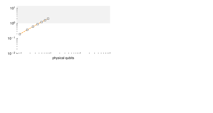
Figure 1: Comparison of the circuit run times and gate counts for the quantum Fourier transform (QFT) and quantum approximate optimization algorithm (QAOA) between neutral atoms and superconducting circuits. The left (right) column corresponds to the QFT (QAOA) and the orange (purple) marker correspond to neutral atoms (superconducting circuits). The circuit run times for both algorithms and various problem instances of different size, $N=9,16,\dots,81$ qubits for the QFT and $N=9,16,\dots,121$ qubits for the QAOA, are given in panels (a) and (c), respectively. The numbers of two- and multi-qubit gates in the corresponding circuits are given in panels (b) and (d), respectively. The data for the squares [circles] is obtained using the standard gate model (SGM) using the gates and times from the standard gate set (SGS) [QSL gate set (QGS)], cf. Table 1. In contrast, the plus signs [crosses] represent the results when the same algorithms are realized in the parity mapping (PM) using the SGS [QGS]. The pentagons correspond to an altered 2D architectures allowing for next-to-nearest neighbor (NNN) coupling between qubits. The run time for each circuit is given in units of typical platform-specific error times. The gray area in panels (a) and (c) indicates where the circuit run times exceeds the error times.

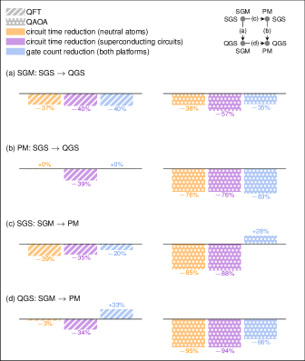
Figure 2: Reduction in weighted circuit run times and (two- and multi-qubit) gate counts for the scenarios and data shown in Fig. 1. In panels (a) and (b) the circuits in the standard gate model (SGM) and parity mapping (PM) are compared when using the “QSL gate set” (QGS) instead of the “standard gate set” (SGS). In panels (c) and (d) the circuits in the SGS and QGS are compared when using the PM instead of the SGM. All presented numbers are the average over problem instances of different sizes, i.e., different numbers of qubits.

II.1 Standard and QSL gate sets

In the SGM, each quantum algorithm is converted into quantum circuits using gates from a universal set of quantum gates. Such a universal set typically contains all the single-qubit gates and at least one entangling two-qubit gate, e.g., the CNOT gate [38]. The row named “standard gate set” in Table 1 summarizes the native universal gate sets and their typical gate times for both platforms at comparable gate fidelities. For neutral atoms, we consider the controlled-Z gate, $\mathrm{CZ}=\mathrm{diag}\{1,1,1,-1\}$, as the typical entangling two-qubit gate. This is a common choice for neutral atoms [20] as it has been successfully used for implementing quantum algorithms [39, 40]. For superconducting circuits, we have chosen the iSWAP-like Sycamore gate as an entangling two-qubit gate, motivated by its short gate time and successful usage in recent quantum advantage experiments with quantum processors based on tunable couplers [8, 9].

In addition, we consider an extended, platform-independent set of quantum gates operated at the QSL (see “QSL gate set” in Table 1). This set consists of all single-qubit gates as well as several multi-qubit gates implementable on both platforms: CZ, CNOT, SWAP, ZZZ, and ZZZZ. The availability of a wider range of gates allows for more flexibility in finding circuit representations with fewer gates and shorter circuit run times. In addition, we also assume that every gate in this set is executed at the QSL, which allows for another speed-up of circuit run times. The run times obtained for the QGS should therefore be viewed as an estimate for the QSL of the circuit itself, i.e., the circuit QSL — provided that no other, potentially faster and/or better suited gates are available . Note that the details regarding the method to determine the QSLs and their results are presented in Secs. IV and V. The row “QSL gate set” in Table 1 summarizes the gates of the extended set and lists the QSL times for both platforms.

Table 1 indicates that absolute circuit run times for neutral atoms will be longer compared to those for superconducting circuits since their elemental gate times differ by more than an order of magnitude. However, in order to ensure a fair comparison of circuit run times the absolute gate times need to be weighted by the finite coherence time and lifetime of qubits and other levels involved in the gate mechanisms.

For neutral atoms, we take both the coherence time of the qubit states, given by the dephasing time $T_{2}^{*}=$4\text{\,}\mathrm{ms}$$ [39], and the lifetime of the Rydberg state, $T_{\mathrm{Ryd}}=$150\text{\,}\mathrm{\SIUnitSymbolMicro s}$$ [39], as typical error time scales against which we compare circuit run times. We take the former as reference for single-qubit gates, since they don’t occupy the Rydberg level ,and the latter for two-qubit gates, where controlled transitions via Rydberg levels constitute the primary gate mechanism . For superconducting circuits, we take their intrinsic $T_{1}$ time, $T_{1}=$15\text{\,}\mathrm{\SIUnitSymbolMicro s}$$ [8], as typical error time scale since it applies for both single- and two-qubit gates. However, note that these choices are rather conservative. For neutral atoms, any two-qubit gate dynamics will naturally also involve the qubit levels, which have much longer coherence times. Weighting two-qubit gates exclusively by the Rydberg lifetime thus overestimates the lifetime-induced error probability. For superconducting circuits, longer $T_{1}$ times up to $500\text{\,}\mathrm{\SIUnitSymbolMicro s}$ have already been reported [44].

II.2 Circuit times in the standard gate model

In the following, we calculate the circuit run times for QFTs and single QAOA steps in the SGM using gates from both the SGS and the QGS. As already outlined above, we assume both hardware platforms to consist of qubits arranged in 2D arrays with only nearest-neighbor connectivity (see Sec. III for details regarding the model). This requires replacing all gates between non-connected qubits with gate sequences between physically connected qubits.

II.2.1 Standard gate set circuits

Using gates from the SGS, the circuit’s gate sequences consist of single-qubit gates plus CZ gates in case of neutral atoms and single-qubit gates plus Sycamore gates in case of superconducting circuits (cf. Table 1). Since the circuit for the QFT does by construction not require any gate between non-neighboring qubits [45], we only replace the controlled-phase gate and SWAP gate by gate sequences from the SGS. The situation changes for the QAOA circuits, as it assumes an all-to-all connected architecture and finding a circuit representation with minimal depth while only requiring nearest-neighbor connectivity is likely NP-hard [46]. As a remedy, we use the open-source pytket compiler [16] to translate the QAOA’s bare quantum circuits to executable quantum circuits that are in agreement with the hardware’s nearest-neighbor connectivity and SGSs. We furthermore use the compiler’s quantum circuit optimization features to optimize the circuits in order to minimize gate counts and circuit depths.

The squares in Fig. 1 (a) and (c) show the resulting run times for quantum circuits corresponding to QFTs and QAOA steps, respectively, when executed on neutral atoms (orange) and superconducting circuits (purple). Within each line, the size of the problem instance increases from the lower left to the upper right. Note that for a fair comparison between platforms, all gate times have been weighted by each platform’s intrinsic error time scales as described previously. Circuits with run times significantly exceeding the platform’s intrinsic, level-dependent error time scales, highlighted by the gray area in Fig. 1 (a) and (c), will most likely yield unreliable results. We observe that despite the different time scales for gates, the weighted circuit run times are almost identical for both platforms and for both the QFT and QAOA, see squares in Fig. 1 (a) and (c), respectively. However, only problem instances with relatively small qubit numbers seem to be currently doable on both platforms.

While the circuit run time is one deciding factor in whether it is feasible on current NISQ hardware, this measure neglects the fact that every gate comes with an intrinsic error probability. Assuming gate errors on the order of $0.1-1\%$, which are realistic both for neutral atoms [20, 40] and superconducting circuits [37], it is clear that also the gate count limits the feasibility of quantum circuits and lower gate counts are thus preferable. To this end, the squares in Fig. 1 (b) and (d) show the number of two-qubit gates required for QFT and single-step QAOA circuits, respectively. Note that circuit representations in terms of the SGS require the same number of two-qubit gates both on neutral atom and superconducting qubit hardware. Hence, both cases are represented by a single line in Figs. 1 (b) and (d).

II.2.2 QSL gate set circuits

The circles in Fig. 1 (a) and (c) show the circuit run times for the same quantum algorithms and complexity levels as used for the squares but when the QGS is employed to generate circuit representations. The corresponding two-qubit gate counts are illustrated by the circles in Fig. 1 (b) and (d). We observe an overall reduction in circuit run times and gate counts for both platforms, both algorithms and any considered problem instance. This improvement is a combined effect of using maximally fast quantum gates at the QSL and taking advantage of the increased flexibility provided by the extended set of gates. Especially the availability of SWAP gates needs to be stressed as it directly reduces the gate count and thus leads to a reduction in circuit run time even without an additional speedup in gate times. In order to quantify the improvements achievable through the QGS, Fig. 2 (a) lists the average reduction in circuit run times and gate counts for each algorithm and platform.

Our analysis demonstrates to which extent circuit run times and gate counts can — from a theoretical perspective — still be improved if standard gates are replaced by an extended gate set with gate times at the QSL. However, even with the improved gate set and its reduction in run time and gate count, most of the quantum circuits, i.e., circles in Fig. 1, remain likely infeasible using current NISQ hardware. Quantum error correction codes could in principle address the issue of circuit run times and gate counts exceeding the limits set by finite lifetimes and gate errors. Nevertheless, since both lifetimes [47, 44] and qubit numbers [48] are constantly increasing, more complex quantum circuits will likely reach the feasible regime in the near future.

II.3 Circuits times in the parity mapping

Besides the representation of quantum algorithms using the SGM, we now consider the representation of the same algorithms within the PM. While the PM was originally designed to tackle combinatorial optimization problems via quantum annealing [27], it can also be utilized for digital quantum optimization algorithms such as QAOA [30] as well as to achieve universal quantum computing [26]. At its core, the PM circumvents the need for long-range interactions between qubits, which in turn renders gates between non-adjacent qubits obsolete. However, this comes at the expense of requiring more physical qubits and many-body constraints on $2\times 2$ plaquettes of qubits as specified in detail in Appendix A.2. Similar to our analysis for the SGM (see Sec. II.2) we use either gates from the SGS or the QGS in the following.

II.3.1 Standard gate set circuits

The plus signs in Fig. 1 (a) [(b)] show the circuit run times [two-qubit gate counts] of QFTs in the PM for the same problem instances as used for the SGM (squares). In both cases and for both platforms, the gates and times of the SGS have been used. We observe a reduction in circuit run times and gate counts for both platforms with the comparison being made with respect to the values for the SGM [see also Fig. 2 (c)]. The same comparison can be done for the QAOA steps with their circuit run times and gate counts given by the plus signs in Fig. 1 (c) and (d), respectively. Regarding single-step QAOA resource requirements, we observe a significant reduction in circuit run times [see also Fig. 2 (c)] due to the constant circuit depth in the PM [29, 30]. However, note that the circuit depth differs for neutral atoms and superconducting circuits due to the different coupling mechanisms between qubits with neutral atoms having the deeper circuits, cf. Appendix A.2. The reduction in circuit run time is accompanied by an increase in two-qubit gate counts compared to the SGM, which we attribute to the decomposition of the constraint gates, cf. Eq. (17), into the natively available gates within each platform.

II.3.2 QSL gate set circuits

The crosses in Fig. 1 show the results for circuit representations in the PM when employing gates and times from the QGS. For the QFT on neutral atoms, we do not observe any further reduction in circuit time or gate counts compared to its representation utilizing the SGS. This is because its circuit representations [49] for neutral atoms contain only single-qubit and CZ gates — gates for which the gate times are identical within the SGS and the QGS. In contrast, for superconducting circuits, we still observe an improvement in circuit time since the CZ gate becomes directly available in the QGS and must no longer be replaced by Sycamore and single-qubit gates. However, the representations in the SGS and QGS only differ by single-qubit gates and hence their two-qubit gate count is identical and also identical to that of the neutral atoms. This is reflected in Fig. 1 (c) by a single line of superimposed plus signs and crosses.

For the single-step QAOA circuits in the PM, we observe a significant reduction both in circuit run time and gate counts on both platforms when the QGS is used instead of the SGS. This is due to the availability of the multi-qubit gates $\mathrm{ZZZ}(\gamma)$ and $\mathrm{ZZZZ}(\gamma)$, cf. Eq. (17), where the gate-count reduction originates from avoiding single- and two-body gate decompositions. In addition, it turns out to be much faster to use control pulses that directly implement these multi-qubit gates as opposed to serially applying control pulses to implement the required single- and two-qubit gates. Figure 2 (b) summarizes the average run time and gate count reductions (in terms of two- and multi-qubit gates) when replacing the SGS with the QGS within the PM.

In contrast to panels (a) and (b) of Fig. 2, where the gate set changes and the circuits stay in the SGM or PM, panels (c) and (d) examine the opposite scenario, i.e., the gate sets are kept constant but the circuit models change. In detail, Fig. 2 (c) and (d) show the average circuit run time and gate count reduction when the SGM is replaced by the PM while the gate set is given by the SGS and QGS, respectively. Especially Fig. 2 (d) needs to be emphasized as it reveals to which extent the PM allows to reduce circuit run times and gate counts compared to representations of the same circuits in the SGM. As mentioned above and detailed in Appendix A.2, the PM-specific improvements come at the only expense of requiring more qubits. For the current state of NISQ hardware and independent from the platform, we believe the SGM to be better suited for QFTs, as more problem instances seem to be feasible, judging by circuit run time and required qubits. In contrast, for QAOA using the QGS, we find the described parity representation of circuits (despite its overhead-induced inferior success probabilities compared to direct SGM-QAOA ) to be an advantageous option, as the run time and gate count is drastically reduced for each QAOA step compared to the SGM. In particular, the need for more PM-QAOA steps compared to SGM-QAOA steps might be compensatable given the resource reduction per PM-QAOA step. Given the ongoing upscaling of quantum computers in terms of qubit numbers, see, e.g., IBM’s quantum roadmap [48], the PM seems to be a viable option for QAOA.

As a final remark, it should be noted that we only discussed optimization problems with all-to-all connectivity, cf. Eq. (12). However, many realistic optimization problems have rather sparse connectivity, which would lead to a significant reduction in required qubits [28] while maintaining its strength of constant circuit depth.

III Modeling neutral atom and superconducting circuit platforms

In Sec. II we have presented the main result of our work — namely a calculation and comparison of circuit run times and gate counts using neutral atoms and superconducting circuits as quantum computing platform. In this section, we now introduce the detailed physical models used for both platforms. Since our focus is the description of dynamics, we focus on the respective Hamiltonians including the various control knobs typically available to steer the systems and implement quantum gates.

III.1 Neutral atoms

Arrays of trapped neutral atoms laser coupled to highly excited Rydberg states are a promising platform for quantum computing [51, 52] and quantum simulation [53] as qubits can for example be encoded in long-lived hyperfine ground states. High-fidelity single-qubit gates can be achieved using microwave fields [54], two-photon Raman transitions [55], or a combination of microwaves and gradient fields for individual-qubit addressing [56, 57, 58]. In contrast, entangling operations between atoms, i.e., many-body gates, are typically realized via strongly interacting Rydberg levels [59, 60] and various control schemes for two- and multi-qubit gates have been experimentally demonstrated [61, 62, 63, 20, 64].

Such gates have been used in recent experiments [39, 40] with up to several hundreds of atoms arranged in a planar geometry. If we consider the smallest building block of such a 2D array, it consists of $N=4$ atoms with each atom described by three relevant levels. In the rotating frame, its Hamiltonian reads ($\hbar=1$)

$$\begin{split}\mathsf{H}(t)&=-\sum_{n=1}^{N}\Delta_{n}(t)\ket{r_{n}}\bra{r_{n}}+\sum_{\begin{subarray}{c}n,m=1\\ n<m\end{subarray}}^{N}V_{nm}\ket{r_{n}r_{m}}\bra{r_{n}r_{m}}\\ &\quad+\frac{1}{2}\sum_{n=1}^{N}\sum_{l=\uparrow,\downarrow}\Big{[}\Omega_{l,n}(t)e^{\textup{i}\varphi_{l,n}}\ket{r_{n}}\bra{l_{n}}+\mathrm{H.c.}\Big{]},\end{split}$$ (1)

where $\ket{\downarrow_{n}}$ and $\ket{\uparrow_{n}}$ denote the qubit levels of the $n$th atom and $\ket{r_{n}}$ its Rydberg level. The Rabi frequencies of the two laser fields coupling the $\ket{\downarrow_{n}}$ and $\ket{\uparrow_{n}}$ states of the $n$th atom to their respective Rydberg level $\ket{r_{n}}$ are denoted by $\Omega_{\downarrow,n}(t)$ and $\Omega_{\uparrow,n}(t)$ . The phases of the respective laser fields are given by $\varphi_{\downarrow,n}(t)$ and $\varphi_{\uparrow,n}(t)$ while $\Delta_{n}(t)$ denotes the detuning of the laser field from the exact transition frequency. We assume $\Delta_{n}(t)$ to be identical for both fields. The van der Waals (vdW) interaction between atom $n$ and $m$ is denoted by $V_{nm}$. Note that in Hamiltonian (1) we have omitted fields responsible for single-qubit gates, i.e., fields coupling the two qubit levels, since our focus is on multi-qubit gates for which the Rydberg levels and their interaction are the primarily gate mechanism.

If not stated otherwise, we assume the laser fields to act identically on all atoms, i.e., $\Omega_{\downarrow,n}(t)=\Omega_{\downarrow}(t)$, $\Omega_{\uparrow,n}(t)=\Omega_{\uparrow}(t)$ and $\varphi_{\downarrow,n}(t)=\varphi_{\downarrow}(t)$, $\varphi_{\uparrow,n}(t)=\varphi_{\uparrow}(t)$ and $\Delta_{n}(t)=\Delta(t)$ for all $n$. In the following, we moreover assume by default a pseudo-2D architecture with $V_{nm}=V$ as described in more detail in Ref. [66]. Effectively, this corresponds to an architecture with equally strong nearest neighbor (NN) and next-to-nearest neighbor (NNN) coupling. However, it should be noted that we do not exploit the NNN couplings when constructing the quantum circuits in Sec. II. It thus does not affect any of the single- or two-qubit gate times presented in Table 1 as these times would be identical for an actual, planar 2D architecture where $V$ is simply the coupling strength between nearest neighbors. The assumption of of the pseudo-2D architecture does only affect the multi-qubit constraint gates $\mathrm{ZZZ}(\gamma)$ and $\mathrm{ZZZZ}(\gamma)$, cf. Eq. (17), which are — within our study — only relevant for the PM using the QGS, cf. the crosses in Fig. 1 (c).

III.2 Superconducting Circuits

Qubits encoded in the lowest energy levels of superconducting circuits are another promising platform for quantum computing [67]. Since their parameters can be to some extent chosen during their fabrication process, superconducting circuits come in various variants and parameter regimes with transmon qubits [68] being currently the most prominent ones for quantum computing. Their qubit levels can be manipulated via microwave fields to either implement single-qubit gates [69, 70] or two-qubit gates [71, 72] with high fidelity. In contrast to neutral atom qubits, which interact directly via their Rydberg levels, qubits encoded in superconducting circuits often interact indirectly via intermediate coupling elements [73]. In an architecture, where such couplers are made tunable [74], the effective interaction strength between the qubits becomes tunable as well. Such qubit architectures have been successfully used in recent quantum advantage experiments [8, 9] and thus are a prototypical NISQ quantum computing platform.

The qubits in such a tunable coupler architecture are arranged on a 2D lattice with nearest-neighbor couplings. In the following, we take the architecture from Ref. [8] as a reference. The smallest building block within such a system consists of $N=4$ qubits. The Hamiltonian for this subsystem reads [8]

$$\begin{split}\mathsf{H}(t)&=\sum_{n=1}^{N}\left[\omega_{n}(t)\mathsf{b}_{n}^{\dagger}\mathsf{b}_{n}-\frac{\alpha_{n}}{2}\mathsf{b}_{n}^{\dagger}\mathsf{b}_{n}^{\dagger}\mathsf{b}_{n}\mathsf{b}_{n}\right]\\ &\quad+\sum_{n=1}^{N}\left(\mathsf{b}_{n}+\mathsf{b}_{n}^{\dagger}\right)\Omega_{n}(t)\cos(\bar{\omega}_{n}(t)t)+\mathsf{H}_{\mathrm{int}}(t)\end{split}$$ (2)

with

$$\begin{split}\mathsf{H}_{\mathrm{int}}(t)&=g_{12}(t)\left(\mathsf{b}_{1}^{\dagger}\mathsf{b}_{2}+\mathsf{b}_{1}\mathsf{b}_{2}^{\dagger}\right)+\frac{g_{12}^{2}(t)}{|\eta|}\mathsf{b}_{1}^{\dagger}\mathsf{b}_{1}\mathsf{b}_{2}^{\dagger}\mathsf{b}_{2}\\ &\quad+g_{23}(t)\left(\mathsf{b}_{2}^{\dagger}\mathsf{b}_{3}+\mathsf{b}_{2}\mathsf{b}_{3}^{\dagger}\right)+\frac{g_{23}^{2}(t)}{|\eta|}\mathsf{b}_{2}^{\dagger}\mathsf{b}_{2}\mathsf{b}_{3}^{\dagger}\mathsf{b}_{3}\\ &\quad+g_{34}(t)\left(\mathsf{b}_{3}^{\dagger}\mathsf{b}_{4}+\mathsf{b}_{3}\mathsf{b}_{4}^{\dagger}\right)+\frac{g_{34}^{2}(t)}{|\eta|}\mathsf{b}_{3}^{\dagger}\mathsf{b}_{3}\mathsf{b}_{4}^{\dagger}\mathsf{b}_{4}\\ &\quad+g_{41}(t)\left(\mathsf{b}_{4}^{\dagger}\mathsf{b}_{1}+\mathsf{b}_{4}\mathsf{b}_{1}^{\dagger}\right)+\frac{g_{41}^{2}(t)}{|\eta|}\mathsf{b}_{4}^{\dagger}\mathsf{b}_{4}\mathsf{b}_{1}^{\dagger}\mathsf{b}_{1},\end{split}$$ (3)

where $\omega_{n}(t)$ is the frequency-tunable level splitting of transmon $n$, $\alpha_{n}$ its anharmonicity and $\mathsf{b}_{n}$ its annihilation operator. The tunable coupling between transmons $n$ and $m$ is denoted by $g_{nm}(t)$ and $\eta$ is the non-linearity of the involved transmons, which is roughly constant $\alpha_{n}\approx\eta$ for all $n$. The time-dependent amplitude and frequency of a local $X$-type control field on transmon $n$, e.g., some microwave field, is denoted by $\Omega_{n}(t)$ and $\bar{\omega}_{n}(t)$, respectively. For numerical reasons, it is advantageous to change into a rotating frame. We change into a rotating frame with frequency $\omega_{\mathrm{rot}}$ via the transformation

$$\mathsf{H}^{\prime}(t) =\mathsf{O}^{\dagger}(t)\mathsf{H}(t)\mathsf{O}(t)-\textup{i}\mathsf{O}^{\dagger}(t)\frac{\mathrm{d}\mathsf{O}(t)}{\mathrm{d}t},$$ (4a)

$$\mathsf{O}(t) =\exp\left\{-\textup{i}\omega_{\mathrm{rot}}\left(\sum_{n=1}^{N}\mathsf{b}_{n}^{\dagger}\mathsf{b}_{n}\right)t\right\}$$ (4b)

and find

$$\begin{split}\mathsf{H}^{\prime}(t)&=\sum_{n=1}^{N}\left[\left(\omega_{n}(t)-\omega_{\mathrm{rot}}\right)\mathsf{b}_{n}^{\dagger}\mathsf{b}_{n}-\frac{\alpha_{n}}{2}\mathsf{b}_{n}^{\dagger}\mathsf{b}_{n}^{\dagger}\mathsf{b}_{n}\mathsf{b}_{n}\right]\\ &\quad+\sum_{n=1}^{N}\frac{1}{2}\left[\mathsf{b}_{n}\left(\bar{\Omega}_{n,\mathrm{re}}(t)+\textup{i}\bar{\Omega}_{n,\mathrm{im}}(t)\right)\right.\\ &\qquad\qquad\left.+\mathsf{b}_{n}^{\dagger}\left(\bar{\Omega}_{n,\mathrm{re}}(t)-\textup{i}\bar{\Omega}_{n,\mathrm{im}}(t)\right)\right]+\mathsf{H}_{\mathrm{int}}(t),\end{split}$$ (5)

where we have introduced the auxiliary control fields

$$\bar{\Omega}_{n,\mathrm{re}}(t) =\mathfrak{Re}\left\{\Omega_{n}(t)e^{-\textup{i}(\omega_{\mathrm{rot}}-\bar{\omega}_{n}(t))t}\right\},$$ (6a)

$$\bar{\Omega}_{n,\mathrm{im}}(t) =\mathfrak{Im}\left\{\Omega_{n}(t)e^{-\textup{i}(\omega_{\mathrm{rot}}-\bar{\omega}_{n}(t))t}\right\}.$$ (6b)

While $\Omega_{n}(t)$ and $\bar{\omega}_{n}(t)$ are the actual physical control fields, we may take $\bar{\Omega}_{n,\mathrm{re}}(t)$ and $\bar{\Omega}_{n,\mathrm{im}}(t)$ as auxiliary control fields which capture the time-dependent nature of $\Omega_{n}(t)$ and $\bar{\omega}_{n}(t)$ in the rotating frame and the latter can be reobtained from $\bar{\Omega}_{n,\mathrm{re}}(t)$ and $\bar{\Omega}_{n,\mathrm{im}}(t)$.

IV Determining quantum speed limits via quantum optimal control

After having introduced the physical model for neutral atoms and superconducting circuits in Sec. III, we now review the basic notion of QSLs in Sec. IV.1 and of quantum optimal control theory in Sec. IV.2 since both build the theoretical, respectively methodical, foundation for the results presented in this work. Our method is described in Sec. IV.3.

IV.1 Quantum speed limits

The notion of quantum speed limits (QSLs) naturally arises in the context of quantum control problems. To this end, let us consider a quantum system described by the Hamiltonian $\mathsf{H}(t)=\mathsf{H}(\{\mathcal{E}_{k}(t)\})$, which depends on a set of control fields, $\{\mathcal{E}_{k}(t)\}$, that can be externally tuned, e.g., by the time-dependent amplitudes, phases or detunings in Eqs. (1) or (5). A quantum control problem is then defined by a set of initial states, $\{\ket{\psi_{l}^{\mathrm{in}}}\}$, that should be transferred into a set of target states, $\{\ket{\psi_{l}^{\mathrm{trgt}}}\}$,

$$\Ket{\psi_{l}^{\mathrm{trgt}}}=\mathsf{U}(T,0;\{\mathcal{E}_{k}(t)\})\Ket{\psi_{l}^{\mathrm{in}}},\quad\forall l,$$ (7)

where $\mathsf{U}(T,0;\{\mathcal{E}_{k}(t)\})$ is the system’s time-evolution operator and $T$ the total time. Any choice of $\{\mathcal{E}_{k}(t)\}$ which fulfills Eq. (7) is considered a solution to the control problem. It is important to note that solutions to quantum control problems are usually not unique. Even for a fixed protocol duration $T$ there typically exist many and often infinite many solutions.

The QSL for a given control problem is defined by the shortest protocol duration $T_{\mathrm{QSL}}$ for which at least one solution exists, i.e., for which at least one set of control fields $\{\mathcal{E}_{k}(t)\}$ exists that fulfills Eq. (7). In the context of quantum computing and the NISQ era, where time is a limited resource due to decoherence, it is desirable to implement quantum gates at the QSL. In order to calculate $T_{\mathrm{QSL}}$ analytically, $\mathsf{U}(T,0;\{\mathcal{E}_{k}(t)\})$ must be analytically calculable for any set $\{\mathcal{E}_{k}(t)\}$ of conceivable control fields — a requirement that typically limits an analytical calculation of $T_{\mathrm{QSL}}$ to simple systems [75].

Besides an analytical determination, there are various methods to approximate $T_{\mathrm{QSL}}$. One prominent method is to calculate a lower bound $T_{\mathrm{bound}}\leq T_{\mathrm{QSL}}$ in order to get an estimate for $T_{\mathrm{QSL}}$ itself. For the simplest case of a state-to-state control problem, lower bounds can be calculated analytically [24]. In contrast, in case of multiple pairs of initial and final states, which describe the implementation of quantum gates, such lower bounds only exist for very simple systems [76]. In most cases, one needs to resort to numerical tools for estimating $T_{\mathrm{QSL}}$. In that context, quantum optimal control theory has proven to be very useful [77] as it not only estimates $T_{\mathrm{QSL}}$ quite accurately but additionally yields the control fields that implement the desired dynamics, i.e., realizing the transition from initial to target states, cf. Eq. (7). Since this is our method of choice, we introduce it in more detail in the following.

IV.2 Quantum optimal control theory

Quantum optimal control theory (OCT) [78] is a toolbox providing analytical and numerical tools that allow to derive optimized control fields which solve a given control problem, e.g., in shortest time or with minimal error. Mathematically, an optimal control problem is formulated by introducing the cost functional

$$\begin{split}J\left[\{\psi_{l}\},\{\mathcal{E}_{k}\},T\right]&=\varepsilon_{T}\left[\{\psi_{l}(T)\}\right]\\ &\quad+\int_{0}^{T}J_{t}\left[\{\psi_{l}(t)\},\{\mathcal{E}_{k}(t)\},t\right]\mathrm{d}t,\end{split}$$ (8)

where $\{\psi_{l}(t)\}$ is a set of time-evolved states and $\{\mathcal{E}_{k}(t)\}$ a set of control fields to be optimized. The error-measure $\varepsilon_{T}$ quantifies the distance between the time-evolved states $\ket{\psi_{l}(T)}=\mathsf{U}(T,0;\{\mathcal{E}_{k}(t)\})\ket{\psi_{l}^{\mathrm{in}}}$ and the desired target states $\ket{\psi_{l}^{\mathrm{trgt}}}$ at the protocol’s final time $T$, cf. Eq. (7). The term $J_{t}$ in Eq. (8) captures time-dependent running costs. In most cases, the error-measure $\varepsilon_{T}$ is the crucial figure of merit. In order to optimize for quantum gates, we use the error-measure [79]

$$\varepsilon_{T}\left[\{\psi_{l}(T)\}\right]=1-\frac{1}{N_{\mathrm{trgt}}}\sum_{l=1}^{N_{\mathrm{trgt}}}\mathfrak{Re}\left\{\Braket{\psi_{l}^{\mathrm{trgt}}}{\psi_{l}(T)}\right\}$$ (9)

and take $\ket{\psi_{l}^{\mathrm{trgt}}}=\mathsf{O}\ket{\psi_{l}^{\mathrm{in}}}$ as the desired target states for the target gate $\mathsf{O}$. The set $\{\psi_{l}^{\mathrm{in}}\}$ runs over the $N_{\mathrm{trgt}}$ logical basis states affected by $\mathsf{O}$ with $N_{\mathrm{trgt}}=4,8,16$ for two-, three- or four-body gates, respectively.

Since the cost functional $J$ is formulated such that smaller values correspond to better solutions of the control problem, solving an optimal control problem becomes essentially a minimization task, i.e., to find a set of control fields $\{\mathcal{E}_{k}^{\mathrm{opt}}(t)\}$ that minimizes $J$, respectively $\varepsilon_{T}$. This is an optimization problem for which several numerical algorithms have been developed [80, 81, 82, 83, 84]. Many of them are readily available in open-source software packages [85, 86, 87, 88, 89].

IV.3 Optimization procedure and method

In the context of determining $T_{\mathrm{QSL}}$ numerically via OCT, we search for the shortest protocol duration $T$ for which the error-measure $\varepsilon_{T}$, cf. Eq. (9), is still sufficiently small. In mathematical terms, we therefore define an error threshold $\varepsilon_{\mathrm{max}}$ and search for the shortest time $T$ for which

$$\underset{\{\mathcal{E}_{k}\}}{\mathrm{min}}\left[\varepsilon_{T}\left[\{\psi_{l}(T)\}\right]\right]\leq\varepsilon_{\mathrm{max}}$$ (10)

has a solution. However, the minimization over all conceivable control fields can not be done numerically — as there are infinitely many fields to check — and thus must be replaced by a sampling over finitely many fields in practice. In order to explore the function space efficiently by finite sampling, optimization algorithm as described in Sec. IV.2 can be used. Since we are interested in the fundamental QSL, we put only minimal limitations — apart from physically motivated limitations on amplitudes — on the form of each control field $\mathcal{E}_{k}(t)$. Hence, we need an optimization algorithm that is capable of exploring a function space of almost arbitrary field shapes.

As our method of choice we use Krotov’s method [90], a gradient-based optimization algorithms for time-continuous control fields. While a more detailed description of Krotov’s method is given in Appendix B, its basic working principle is outlined in the following. It consists of an iterative update of the control fields $\{\mathcal{E}_{k}(t)\}$. Starting from a set of guess control fields $\{\mathcal{E}_{k}^{0}(t)\}$, Krotov’s method updates them until either $\varepsilon_{T}\leq\varepsilon_{\mathrm{max}}$ or a maximum number of iterations is reached. This procedure can be viewed as a local but structured search within the space of all conceivable sets of control fields — the so-called control landscape. The locally searched area is thereby determined by the choice of the guess fields $\{\mathcal{E}_{k}^{0}(t)\}$, which set the initial starting point of the search. While the local nature of this search might appear contradicting to the global search required for evaluating Eq. (10), it can be turned into an approximate global search by using various sets of randomized guess fields. The combined effect of all these local searches “cover” a larger fraction of the control landscape. The total procedure for approximating $T_{\mathrm{QSL}}$ using this method is thus to start with a protocol duration $T$ for which the optimization algorithm finds solutions, i.e., optimized fields giving rise to $\varepsilon_{T}\leq\varepsilon_{\mathrm{max}}$, and then to consecutively lower $T$ until none of the various sets of randomized guess fields finds a solution anymore. Appendix C summarizes the details regarding the generation of random guess fields as well as each field’s parametrization within Krotov’s method.

Similar application of numerical optimal control techniques have previously shown excellent agreement with analytically provable QSLs [91, 92]. At worst, this method could overestimate the actual QSLs, in which case the actual QSLs would be even smaller and the circuit and gate times in Sec. II that use the QGS would be even better.

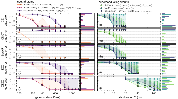
Figure 3: Overview of the QSLs for the various gates of the “QSL gate set” (QGS) in Table 1. The left (right) column shows the results for neutral atoms (superconducting circuits) for three different configurations of control fields (specified in the main text), respectively. Each marker represents the gate error $\varepsilon_{T}$, cf. Eq. (9), after either reaching $\varepsilon_{T}\leq\varepsilon_{\mathrm{max}}=10^{-3}$ or $1500$ iterations of Krotov’s method, cf. Appendix B, after starting from a set of random guess fields generated via Eq. (22). While the lines connect the lowest errors reached for each gate time $T$ within a given field configuration, the shaded background color indicates the range between the lowest and highest error. The marker density is shown at the right side of each panel as a histogram. The parameters for neutral atoms are $V/2\pi=$40\text{\,}\mathrm{MHz}$$, $0\leq\Omega_{\downarrow}(t),\Omega_{\uparrow}(t)\leq\Omega_{\mathrm{max}}=0.1V$ and $|\Delta(t)|\leq\Delta_{\mathrm{max}}=0.3V$. The parameters for superconducting circuits are $-$40\text{\,}\mathrm{MHz}$\leq g_{nm}(t)/2\pi\leq$5\text{\,}\mathrm{MHz}$$, $$6700\text{\,}\mathrm{MHz}$\lesssim\omega_{n}(t)\lesssim$7100\text{\,}\mathrm{MHz}$$ (exact values depending on $n$ and taken from Ref. [8]) and $-$50\text{\,}\mathrm{MHz}$\leq\bar{\Omega}_{n,\mathrm{re}}(t),\bar{\Omega}_{n,\mathrm{im}}(t)\leq$50\text{\,}\mathrm{MHz}$$. The anharmonic ladder for each transmon has been truncated after five levels with population in the highest level suppressed during optimization. The optimization results for $\mathrm{ZZZ}(\gamma)$ and $\mathrm{ZZZZ}(\gamma)$, cf. Eq. (17), have been obtained for the maximally entangling gate at $\gamma=\pi/4$. The results for the CNOT gate on neutral atoms have been obtained using site-dependent control fields for each atom.

V Benchmarking quantum gate times on 2D architectures

In this final section, we now present the detailed results regarding the QSLs obtained via methods described in Sec. IV for the various gates listed in Table 1 and have been used to calculate the circuit run times in Sec. II.

V.1 Neutral atoms

In this section, we determine the QSLs for different gates on neutral atoms by utilizing the control knobs available in Hamiltonian (1). To this end, we set the vdW interaction strength between Rydberg levels to $V/2\pi=$40\text{\,}\mathrm{MHz}$$ and assume a maximally achievable Rabi frequency of $\Omega_{\mathrm{max}}/2\pi=0.1V=$4\text{\,}\mathrm{MHz}$$ for both $\Omega_{\downarrow}(t)$ and $\Omega_{\uparrow}(t)$ as well as $\Delta_{\mathrm{max}}/2\pi=0.3V=$12\text{\,}\mathrm{MHz}$$ for $|\Delta(t)|$. These parameters are in the same regime than those reported in recent experiments [93, 20, 39].

The markers in Fig. 3 (left column) show the achievable gate error $\varepsilon_{T}$, cf. Eq. (9), for various gates and various gate times $T$ on neutral atoms. Each individual marker thereby indicates the result of a single optimization with Krotov’s method [cf. Appendix (B)] i.e., the final error $\varepsilon_{T}$ after $1500$ iterations when starting from random guess fields generated via Eq. (22). In the following we set $\varepsilon_{\mathrm{max}}=10^{-3}$ for all gates and stop any optimization as soon as this threshold is reached.

V.1.1 Two-qubit gates

Figure 3 (a) shows the results for a CZ gate for three different, paradigmatic configurations of control fields. The circles correspond to the “parallel” configuration where all five possible control fields $\Omega_{\downarrow}(t),\Omega_{\uparrow}(t),\varphi_{\downarrow}(t),\varphi_{\uparrow}(t)$ and $\Delta(t)$ have been optimized. In contrast, the crosses correspond to the “phase” configuration, where only $\varphi_{\uparrow}(t)$ has been optimized while $\Omega_{\uparrow}(t)=\Omega_{\mathrm{max}}$, $\Delta(t)=\Delta_{\mathrm{max}}$ and $\Omega_{\downarrow}(t)=\varphi_{\downarrow}(t)=0$ have been kept fixed. In both cases, we obtain a QSL of $T_{\mathrm{QSL}}^{\mathrm{CZ}}=$350\text{\,}\mathrm{ns}$$. The third field configuration, which we called “sequential” configuration (diamonds), consists of a sequential use of $\Omega_{\downarrow}(t),\varphi_{\downarrow}(t)$ and $\Omega_{\uparrow}(t),\varphi_{\uparrow}(t)$, i.e., the first half of the protocol we have $\Omega_{\uparrow}(t)=\varphi_{\uparrow}(t)=0$ and in the second half $\Omega_{\downarrow}(t)=\varphi_{\downarrow}(t)=0$. This configuration is inspired by an adiabatic protocol for implementing $\mathrm{ZZZZ}(\gamma)$ gates, cf. Eq. (17) and Ref. [66]. Its QSL $T_{\mathrm{QSL}}^{\mathrm{CZ}}=$700\text{\,}\mathrm{ns}$$ is twice as long compared to the other two configurations.

In order to compare the results from the three configurations in terms of how successful the optimization has been in finding solutions, the histogram on the right side of Fig. 3 (a) provides the probability density for obtaining final errors $\varepsilon_{T}$ within certain ranges. For obtaining a solution with errors $\varepsilon_{T}\leq\varepsilon_{\mathrm{max}}$, we find the lowest probability for the “sequential” configuration (diamonds) — coinciding with the highest QSL — and the highest and almost identical probability for the other two configurations. Among those two, the “phase” configuration (crosses) needs to be emphasized in particular. From a physical perspective, setting $\Omega_{\downarrow}(t)$ and $\varphi_{\downarrow}(t)$ to zero automatically ensures that $\ket{\downarrow\downarrow}$ is mapped onto itself — as required by the CZ gate. This is not automatically guaranteed by the other two configurations and the optimization needs to explicitly ensure it and therefore needs to solve a slightly more complex optimization problem. However, the advantage of having one basis state automatically mapped correctly does not translate into an advantage regarding the QSL of $T_{\mathrm{QSL}}^{\mathrm{CZ}}=$350\text{\,}\mathrm{ns}$$ or the reachable error in general. Interestingly, both the “parallel” and “phase” configurations yield the same achievable lowest errors for each gate time $T$. This is visually highlighted by the lines connecting the lowest errors per $T$ in Fig. 3 (a). Moreover, it should be stressed that these errors $\varepsilon_{T}$ are reached for almost every set of initial guess fields, i.e., independent of the initial starting point within the problem’s control landscape, and obtained independently for both configurations. This supports the conjecture that $T_{\mathrm{QSL}}^{\mathrm{CZ}}=$350\text{\,}\mathrm{ns}$$ is the actual QSL for a CZ gate and generally validates our method in determining the QSL. From an optimal control perspective, it is interesting to see that the flexibility originating from the extended set of available control fields in the “parallel” configuration can not be turned into an advantage in error or time compared to the “phase” configuration. From a practical perspective, the latter is advantageous for experimental realizations as it requires fewer physical resources.

While the three configurations discussed so far should only be viewed as examples, we did not find any configuration giving rise to faster CZ gates. Hence, we assume $T_{\mathrm{QSL}}^{\mathrm{CZ}}=$350\text{\,}\mathrm{ns}$$ to be the fundamental QSL across all configurations. A natural comparison for $T_{\mathrm{QSL}}^{\mathrm{CZ}}$ with a value from the literature would be the gate time from the analytical protocol introduced in Ref. [20], especially because it uses the same control fields as the “phase” configuration to implement the gate. For our parameters, we find $T_{\mathrm{lit}}^{\mathrm{CZ}}\approx$340\text{\,}\mathrm{ns}$$ as analytical gate time, which we assume identical with our QSL $T_{\mathrm{QSL}}^{\mathrm{CZ}}=$350\text{\,}\mathrm{ns}$$ given the rather coarse sampling of gate times $T$ in Fig. 3 (a). However, it should be noted that the analytical protocol of Ref. [20] implements a CZ gate only up to local operations — operations that are already contained in our optimized gate protocols at the QSL. Nevertheless, for a fair comparison of analytical and QSL gate times, as needed in Sec. II, as well as for simplicity, we set both times to $350\text{\,}\mathrm{ns}$ in Table 1.

The remaining panels (b)-(e) in the left column of Fig. 3 show the results for other gates from the QGS of Table 1. The results for a CNOT gate are shown in panel (b). It is the only gate for neutral atoms (among those we considered) that requires individual instead of global fields, i.e., it is the only gate for which we did not assume $\Omega_{\downarrow,n}(t)=\Omega_{\downarrow}(t),\Omega_{\uparrow,n}(t)=\Omega_{\uparrow}(t),\varphi_{\downarrow,n}(t)=\varphi_{\downarrow}(t),\varphi_{\uparrow,n}(t)=\varphi_{\uparrow}(t)$ and $\Delta_{n}(t)=\Delta(t)$ for all $n$ but actually assume individual fields with unique field shapes directed at each atom. We nevertheless consider the same three field configurations as for the CZ gate in panel (a) but now applied to the individual fields $\Omega_{\downarrow,n}(t),\Omega_{\uparrow,n}(t),\varphi_{\downarrow,n}(t),\varphi_{\uparrow,n}(t)$ and $\Delta_{n}(t)$ instead of their global versions. Even with this more general setting of control fields, we find only the “parallel” configuration (circles) to allow for the realization of a CNOT gate with a QSL of $T_{\mathrm{QSL}}^{\mathrm{CNOT}}=$300\text{\,}\mathrm{ns}$$. In contrast, the “phase” and “sequential” configurations do not allow to realize a CNOT gate at all. These results demonstrate that CNOT gates can be implemented using exclusively the site-dependent laser couplings of the qubit and Rydberg levels and no control knobs for single-qubit gates. However, an experimentally more convenient option, requiring no full site-dependent control of coupling qubit to Rydberg states, is to realize CZ gates with global laser pulses and convert them into CNOTs via local operations. We nevertheless include the CNOT gate and its QSL for completeness in our analysis as well as in the QGS in Table 1 but exclude it from any quantum circuit for neutral atoms in Sec. II for the reasons just mentioned.

Figure 3 (c) shows the results for a SWAP gate. Like for the CNOT gate, we find the “parallel” configuration — assuming again global fields that are identical for each atom — to be the only one capable of realizing a SWAP gate. We obtain $T_{\mathrm{QSL}}^{\mathrm{SWAP}}=$400\text{\,}\mathrm{ns}$$ as its QSL. The other two configurations are not capable of realizing SWAP gates. However, since the SWAP gate, in contrast to the CNOT gate, can be realized with global control fields, we believe it to be experimentally feasible and thus include it as a viable gate in the QGS in Table 1.

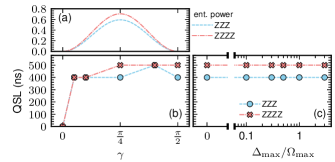
Figure 4: Panel (a) shows the entanglement power [94] of the three- and four-qubit constraint gates $\mathrm{ZZZ}(\gamma)$ and $\mathrm{ZZZZ}(\gamma)$, cf. Eq. (17), as a function of $\gamma$. In contrast, panels (b) and (c) examine the QSLs for these gates under various conditions on neutral atoms. In panel (b), the dependence of the QSL on the parameters $\gamma$ is shown. In panel (c), the impact of $\Delta_{\mathrm{max}}/\Omega_{\mathrm{max}}$ is visualized. In the latter case, we have $\gamma=\pi/4$ and a fixed $\Omega_{\mathrm{max}}$ while $\Delta_{\mathrm{max}}$ is modified. The QSLs in panels (b) and (c) have been determined using the parameters and “phase” configuration described in Fig. 3.

V.1.2 Three- and four-qubit constraint gates

So far, we have discussed the results for two-qubit gates in Fig. 3 (a)-(c). These gates and their respective QSLs have been used in determining the quantum circuits and calculating the corresponding circuit run times in Sec. II — especially for those circuits in the SGM discussed in Sec. II.2. In contrast, for QAOA circuits in the PM [29], circuit representations without two-qubit gates exist, e.g., when the required three- and four-qubit constraint gates $\mathrm{ZZZ}(\gamma)$ and $\mathrm{ZZZZ}(\gamma)$, cf. Eq. (17), are available natively and thus must not be decomposed into single- and two-qubit gates. In the following, we determine and discuss their QSLs.

It should first be noted that, from an algorithmic point of view, it is irrelevant whether, e.g., $\mathrm{ZZZ}(\gamma)$ or $e^{\textup{i}\alpha}\mathrm{ZZZ}(\gamma)$, with $\alpha$ some arbitrary phase, is realized in experiments. The latter just changes the global phase of the quantum state during circuit execution. The same holds for the $\mathrm{ZZZZ}(\gamma)$ gate. In both cases, we may choose $\alpha$ arbitrarily but, for practical reasons, choose it such that the states $\ket{\downarrow\downarrow\downarrow}$ and $\ket{\downarrow\downarrow\downarrow\downarrow}$ do not acquire a phase from the respective constraint gates. In the following, we therefore consider the phase-shifted constraint gates

$$e^{\textup{i}\gamma}\mathrm{ZZZ}(\gamma),\qquad e^{-\textup{i}\gamma}\mathrm{ZZZZ}(\gamma),$$ (11)

instead of the ones from Eq. (17).

In the context of QAOA circuits in the PM, these constraint gates need to be realized for various $\gamma$, cf. Eq. (14). However, since we can not determine their QSL for each value of $\gamma$, we first analyze the gate’s entangling power [94] as a function of $\gamma$ in Fig 4 (a). We observe maximal entangling power for $\gamma=\pi/4$ for both $\mathrm{ZZZ}(\gamma)$ and $\mathrm{ZZZZ}(\gamma)$ and thus decide to first benchmark their QSLs for that particular value as we expect the control problem in that case to be the hardest to solve and consequently the QSLs to be the largest.

Figure 3 (d) and (e) show the optimization results for the phase-shifted constraint gates $\mathrm{ZZZ}(\gamma)$ and $\mathrm{ZZZZ}(\gamma)$, cf. Eq. (11), for $\gamma=\pi/4$, respectively. We use the same three configurations of control fields as for the two-qubit gates in panels (a)-(c) and find all configurations to be capable of implementing the constraint gates but observe the best performance for the “parallel” and “phase” configuration. While both configurations yield the same QSLs of $T_{\mathrm{QSL}}^{\mathrm{ZZZ}}=$400\text{\,}\mathrm{ns}$$ and $T_{\mathrm{QSL}}^{\mathrm{ZZZZ}}=$500\text{\,}\mathrm{ns}$$ for $\mathrm{ZZZ}(\gamma)$ and $\mathrm{ZZZZ}(\gamma)$, respectively, the “phase” configuration exhibits the better convergence behavior. Like for the CZ gate in Fig. 3 (a), we observe every set of guess fields for this configuration to reliably converge towards the same final error $\varepsilon_{T}$ for every $T$. Since the “parallel” configuration yields the same achievable errors as a function of gate time $T$ and uses by definition a different control strategy than the “phase” configuration, we believe to have reliably identified the QSLs for the constraint gates. In terms of experimental feasibility, the “phase” configuration is advantageous as it requires fewer hardware and control resources.

The fact that using $\varphi_{\uparrow}(t)$ as the only time-dependent control field suffices for implementing $\mathrm{ZZZ}(\gamma)$ or $\mathrm{ZZZZ}(\gamma)$ originates from considering the gates’ phase-shifted versions of Eq. (11). In detail, since the states $\ket{\downarrow\downarrow\downarrow}$ and $\ket{\downarrow\downarrow\downarrow\downarrow}$ are the only states among the $8$ or $16$ basis states of $\mathrm{ZZZ}(\gamma)$ or $\mathrm{ZZZZ}(\gamma)$ that technically require non-zero $\Omega_{\downarrow}(t)$ and $\varphi_{\downarrow}(t)$ in order to be phase-configurable, we simply avoid this requirement by considering the gates’ phase-shifted version. For the remaining $7$ or $15$ basis states, which all have at least one atom initially in the $\ket{\uparrow}$ state, the phase $\varphi_{\uparrow}(t)$ together with a constant $\Omega_{\uparrow}(t)=\Omega_{\mathrm{max}}$ is sufficient to correctly adjust all phases. The “phase” configuration thus represents a hardware-efficient control scheme to realize fast $\mathrm{ZZZ}(\gamma)$ and $\mathrm{ZZZZ}(\gamma)$ gates.

Our results furthermore reveal that the “sequential” configuration, which was recently introduced in Ref. [66] and designed to implement high-fidelity $\mathrm{ZZZZ}(\gamma)$ gates, seems not to be ideal when it comes to gate time as its configuration-specific QSL is roughly twice as long as the QSLs for the other configurations. However, it should be noted that a comparison of the protocol from Ref. [66] with protocols at the QSL is not a fair comparison. On the one hand, the control scheme of Ref. [66] is based on adiabaticity — a regime that we are far away from in our numerical calculations. On the other hand, while the parameter $\gamma$ is a tunable variable in the adiabatic control scheme, the results in Fig. 3 (d) and (e) are only valid for $\gamma=\pi/4$. If gates with a different $\gamma$ are required, one explicitly needs to optimize control fields for that purpose. While it is beyond the scope of this work to examine whether there exists an analytical control scheme with configurable $\gamma$ at the QSL, in the following, we nevertheless provide an analysis of the QSLs for $\mathrm{ZZZ}(\gamma)$ and $\mathrm{ZZZZ}(\gamma)$ beyond $\gamma=\pi/4$. In detail, after having identified the “phase” configuration as the most reliable configuration to determine a gate’s QSL, we provide the QSLs for other $\gamma$ values in Fig. 4 (b). We find the QSLs to be almost constant for $\gamma>0$ and only zero for $\gamma=0$, in which case $\mathrm{ZZZ}(\gamma)$ and $\mathrm{ZZZZ}(\gamma)$ coincide with the identity operation. Interestingly, we do not observe a decrease in the QSLs for $\gamma=\pi/2$ in which case the constraint gates are no longer entangling, cf. Fig. 4 (a), and should therefore theoretically be implementable with local operations only. We suspect that we do not see a decrease of the QSLs since we do not consider any control fields for local operations in Hamiltonian (1) and thus need to implement the local gates by means of the Rydberg levels.

We moreover analyze the dependence of the QSLs on the ratio $\Delta_{\mathrm{max}}/\Omega_{\mathrm{max}}$ in Fig. 4 (c). Surprisingly, we observe the QSLs for both $\mathrm{ZZZ}(\gamma)$ and $\mathrm{ZZZZ}(\gamma)$ to be independent on this ratio and find $\Delta_{\mathrm{max}}=0$ to be a viable option.

In general, we observe that the QSLs for $\mathrm{ZZZ}(\gamma)$ and $\mathrm{ZZZZ}(\gamma)$ are only slightly larger than those of the two-qubit gates. In view of quantum circuits for PM-QAOA, where such constraint gates are required, it is thus advantageous to have these gates natively available, since their representation via single- and two-qubit gates [29] consumes significantly more time. This effect can be seen in Fig. 1 (c), where the plus signs illustrate the data for constraint gates expanded in single- and two-qubit gates and the crosses for the usage of native constraint gates. One possible explanation for the short QSLs for $\mathrm{ZZZ}(\gamma)$ and $\mathrm{ZZZZ}(\gamma)$ compared to those of the two-qubit gates might be that the permutation symmetry of atoms within the pseudo-2D architecture [66], i.e., $V_{nm}=V$, matches the permutation symmetry of the gate operation itself.

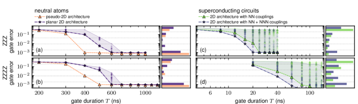
Figure 5: Overview of different QSLs similar to Fig. 3 but exclusively for the three- and four-qubit constraint gates $\mathrm{ZZZ}(\gamma)$ and $\mathrm{ZZZZ}(\gamma)$, cf. Eq. (17). The left column shows results for neutral atoms, obtained using the “phase” configuration of Fig. 3, for the pseudo-2D architecture (triangles) and an actual, planar 2D architecture (stars). The right column compares the results for superconducting circuits using the “no-X” configuration from Fig. 3. The data correspond to the physical architecture of Ref. [8] where only nearest neighbor (NN) couplings between qubits are present (triangles) and where diagonal couplings, i.e., next-to-nearest neighbor (NNN) couplings, are added (stars).

At last, we therefore examine the impact of the pseudo-2D architecture onto the constraint gates $\mathrm{ZZZ}(\gamma)$ and $\mathrm{ZZZZ}(\gamma)$. For the three- and four-qubit constraint gates, the change to an actual, planar 2D architecture implies that while the couplings between nearest neighbors remain $V$, diagonal couplings, i.e., couplings between next-to-nearest neighbors or, in other words, qubits on opposite edges of a $2\times 2$ square plaquette, are replaced by $V/8$. The stars in Fig. 5 (a) and (b) show the corresponding results for $\mathrm{ZZZ}(\gamma)$ and $\mathrm{ZZZZ}(\gamma)$ gates and $\gamma=\pi/4$, respectively. While their QSLs within the pseudo-2D architecture are $T_{\mathrm{QSL}}^{\mathrm{ZZZ}}=$400\text{\,}\mathrm{ns}$$ and $T_{\mathrm{QSL}}^{\mathrm{ZZZZ}}=$500\text{\,}\mathrm{ns}$$, they become $T_{\mathrm{QSL},\mathrm{2D}}^{\mathrm{ZZZ}}=T_{\mathrm{QSL},\mathrm{2D}}^{\mathrm{ZZZZ}}=$600\text{\,}\mathrm{ns}$$ in the actual, planar 2D architecture. Interestingly, this corresponds only to a relatively small increase in the QSLs for both gates. A possible explanation might be that the gate speed for neutral atoms is primarily determined by the maximal Rabi frequency $\Omega_{\mathrm{max}}$, which is identical for both examples, and not so much by the interatomic interaction strength, which is different for both architectures.

Although we believe the pseudo-2D architecture to be viable in experiments due to the great flexibility to arrange neutral atoms [95], we nevertheless take the QSLs for the actual, planar 2D architecture to be the reference gate times within the QGS in Table 1 and Sec. II. However, recall that the constraint gates are — within our study — only relevant for the QAOA circuits in the PM, cf. Fig. 1 (c). In order to nevertheless allow for a comparison of the run times in the actual, planar 2D architecture (orange crosses) with those using the pseudo-2D architecture, we add the latter as orange pentagons to Fig. 1 (c).

V.2 Superconducting circuits

Similar to neutral atoms in Sec. V.1, we now determine and analyze the QSLs for the same quantum gates but for superconducting circuits. The available control knobs to implement these gates are the tunable qubit frequencies $\omega_{n}(t)$, the tunable coupling strength $g_{nm}(t)$ between qubits and the (auxiliary) X-type local control fields $\bar{\Omega}_{n,\mathrm{re}}(t)$ and $\bar{\Omega}_{n,\mathrm{im}}(t)$ in Hamiltonian (5). In order to remain experimentally realistic, we take parameters from Ref. [8]. To this end, we single out a $2\times 2$ plaquette consisting of four qubits from the generally larger 2D architecture. We take the qubit frequencies and their tunable range to be given by $$6700\text{\,}\mathrm{MHz}$\lesssim\omega_{n}(t)\lesssim$7100\text{\,}\mathrm{MHz}$$ and their anharmonicities given by $\alpha_{n}\approx$200\text{\,}\mathrm{MHz}$$, with exact values depending on $n$. The tunable coupling strength is given by $-$40\text{\,}\mathrm{MHz}$\leq g_{nm}(t)\leq$5\text{\,}\mathrm{MHz}$$, as reported in Ref. [8]. Moreover, we assume the (auxiliary) X-type control fields $\bar{\Omega}_{n,\mathrm{re}}(t)$ and $\bar{\Omega}_{n,\mathrm{im}}(t)$, which encode the physical X-type control fields $\Omega_{n}(t)$ and their tunable driving frequencies $\bar{\omega}_{n}(t)$, to satisfy $-$50\text{\,}\mathrm{MHz}$\leq\bar{\Omega}_{n,\mathrm{re}}(t),\bar{\Omega}_{n,\mathrm{im}}(t)\leq$50\text{\,}\mathrm{MHz}$$.

V.2.1 Two-qubit gates

Figure 3 (f) shows results for a CZ gate on superconducting circuits using three different configurations of control fields — different, of course, from those used for neutral atoms. In the “full” configuration (circles), all available control fields, $\omega_{n}(t),g_{nm}(t),\bar{\Omega}_{n,\mathrm{re}}(t)$ and $\bar{\Omega}_{n,\mathrm{im}}(t)$, are time-dependent and being optimized. In the “no-X” configuration (crosses), only $\omega_{n}(t)$ and $g_{nm}(t)$ are optimized while the X-type control fields are set to zero, $\bar{\Omega}_{n,\mathrm{re}}(t)=\bar{\Omega}_{n,\mathrm{im}}(t)=0$. At last, in the “interaction” configuration only $\omega_{n}(t)$ is time-dependent and optimized while $g_{nm}(t)=-$40\text{\,}\mathrm{MHz}$=g_{\mathrm{max}}$ is set to its maximum magnitude and $\bar{\Omega}_{n,\mathrm{re}}(t)=\bar{\Omega}_{n,\mathrm{im}}(t)=0$. For the CZ gate in Fig. 3 (f), we observe all three configurations to indicate the same QSL of $T_{\mathrm{QSL}}^{\mathrm{CZ}}=$10\text{\,}\mathrm{ns}$$. In terms of convergence behavior, the “interaction” configuration shows the best performance as indicated by the probability density on the right side of Fig. 3 (f). In general, the three configurations show slightly worse convergence behavior than the three configurations for the neutral atoms, cf. Fig. 3 (a). Nevertheless, since all three configurations indicate the same QSL and, in general, yield the same achievable error $\varepsilon_{T}$ depending on $T$, we believe our method to determine the QSL to yield reliable results also for superconducting circuits and conjecture $T_{\mathrm{QSL}}^{\mathrm{CZ}}=$10\text{\,}\mathrm{ns}$$ to be the fundamental QSL for CZ gates. While there are reference implementations for CZ gates on similar architectures with tunable couplers [74, 72, 96, 97], none of these architectures matches our architecture and parameter regime. Hence, we compare our QSL to the gate time of the fastest two-qubit gate, the Sycamore gate, reported in Ref. [8]. We find $T_{\mathrm{QSL}}^{\mathrm{CZ}}=$10\text{\,}\mathrm{ns}$$ to be slightly faster than $T_{\mathrm{lit}}^{\mathrm{Syc.}}=$12\text{\,}\mathrm{ns}$$ [37].

In Fig. 3 (g), the results for a CNOT gate are shown using the same three configuration as for the CZ gate. We find only the “full” configuration to be capable of realizing a CNOT gate, yielding the QSL $T_{\mathrm{QSL}}^{\mathrm{CNOT}}=$14\text{\,}\mathrm{ns}$$, while the other two configuration are not capable of it. Among the available control knobs, the X-type control fields $\bar{\Omega}_{n,\mathrm{re}}(t)$ and $\bar{\Omega}_{n,\mathrm{im}}(t)$ are crucial for a CNOT gate to be feasible. For the SWAP gate, we again find all three configuration to converge, cf. Fig. 3 (h), with the “no-X” and “interaction” configuration showing the best convergence behavior. We find a QSL of $T_{\mathrm{QSL}}^{\mathrm{SWAP}}=$12\text{\,}\mathrm{ns}$$.

V.2.2 Three- and four-qubit constraint gates

We now turn towards the three- and four-qubit constraint gates $\mathrm{ZZZ}(\gamma)$ and $\mathrm{ZZZZ}(\gamma)$. However, note that in the following and in contrast to neutral atoms, we do not consider their phase-shifted versions, cf. Eq. (11), but their original versions, cf. Eq. (17).

Figure 3 (i) and (j) show the results for the constraint gates $\mathrm{ZZZ}(\gamma)$ and $\mathrm{ZZZZ}(\gamma)$, respectively. We use the same three configurations of control fields as for the two-qubit gates of panels (f)-(h). We observe the “interaction” configuration to have the best convergence behavior while the “no-X” configuration gives in both cases rise to the shortest QSLs of $T_{\mathrm{QSL}}^{\mathrm{ZZZ}}=$24\text{\,}\mathrm{ns}$$ and $T_{\mathrm{QSL}}^{\mathrm{ZZZZ}}=$80\text{\,}\mathrm{ns}$$ for $\mathrm{ZZZ}(\gamma)$ and $\mathrm{ZZZZ}(\gamma)$, respectively. Both QSLs have been determined for $\gamma=\pi/4$. The QSL for $\mathrm{ZZZ}(\gamma)$ has thereby been confirmed independently by both the “full” and “no-X” configurations as both yield almost identical achievable errors $\varepsilon_{T}$ as a function of gate time $T$. We thus assume the QSL $T_{\mathrm{QSL}}^{\mathrm{ZZZ}}=$24\text{\,}\mathrm{ns}$$ to be well backed up. The situation is different for $\mathrm{ZZZZ}(\gamma)$, for which we observe very different convergence behaviors for the three configurations, cf. Fig. 3 (j). While the “no-X” configuration yields the shortest QSL of $T_{\mathrm{QSL}}^{\mathrm{ZZZZ}}=$80\text{\,}\mathrm{ns}$$, the “full” configuration shows slightly better performance for $T<T_{\mathrm{QSL}}^{\mathrm{ZZZZ}}$, which might suggest that even shorter gate protocols for $\mathrm{ZZZZ}(\gamma)$ may exist but our method did not find them due, e.g., limited numbers of guess fields for exploring the control landscape. In the following, as well as for the calculation of circuit run times in Sec. II, we nevertheless assume $T_{\mathrm{QSL}}^{\mathrm{ZZZZ}}=$80\text{\,}\mathrm{ns}$$ to be the QSL for the $\mathrm{ZZZZ}(\gamma)$ gate as it is the fastest gate time $T$ among the three configurations of control fields for which Krotov’s method was able to find a solution with $\varepsilon_{T}\leq\varepsilon_{\mathrm{max}}$.

Interestingly, while we observe the QSLs for $\mathrm{ZZZ}(\gamma)$ and $\mathrm{ZZZZ}(\gamma)$ to be almost identical for neutral atoms and only slightly longer than the QSLs for the two-qubit gates, we observe the same only for the $\mathrm{ZZZ}(\gamma)$ gate for superconducting circuits. The $\mathrm{ZZZZ}(\gamma)$ gate has a much longer QSL compared to the other QSLs on that platform. To rigorously decide whether this is due to the non-ideal convergence behavior observed in Fig. 3 (j) or has some deeper physical origin is beyond the scope of this study. In an attempt to tackle this question nevertheless, we consider the scenario of having additional diagonal couplings, i.e., next-to-nearest neighbor couplings, among the transmons in the superconducting circuit architecture. For Hamiltonian (3), this implies adding two additional rows with couplings $g_{13}(t)$ and $g_{24}(t)$ in the same form as the already present couplings $g_{12}(t),g_{23}(t),g_{34}(t)$ and $g_{41}(t)$. This scenario is inspired by the pseudo-2D architecture for neutral atoms, which also exhibits identical nearest neighbor (NN) and next-to-nearest neighbor (NNN) couplings and where having these couplings is advantageous. Figure 5 (c) and (d) show the results for the two cases with only NN couplings (triangles) and with NN plus NNN couplings (stars). Besides observing much better convergence properties for the latter case, we also obtain improved QSLs of $T_{\mathrm{QSL},\mathrm{NNN}}^{\mathrm{ZZZ}}=$20\text{\,}\mathrm{ns}$$ and $T_{\mathrm{QSL},\mathrm{NNN}}^{\mathrm{ZZZZ}}=$60\text{\,}\mathrm{ns}$$ for the $\mathrm{ZZZ}(\gamma)$ and $\mathrm{ZZZZ}(\gamma)$ gate, respectively. However, despite improvements in this scenario, the QSL of the $\mathrm{ZZZZ}(\gamma)$ gate does not get close to the QSL of the $\mathrm{ZZZ}(\gamma)$ gate as it does for neutral atoms. The presence of NNN couplings might therefore be just a partial explanation of the QSL differences for the constraint gates between neutral atoms and superconducting circuits. Despite the scenario with NNN couplings not reflecting the actual architecture for superconducting circuits, we nevertheless add the circuit run times for the QAOA circuits in the PM using these faster constraint gates to Fig. 1 (c) for reference purposes as purple pentagons.

VI Conclusions

In this study, we have determined the QSLs for several common two-qubit and two specific multi-qubit quantum gates for two promising quantum computing platforms that allow for a 2D arrangement of qubits — neutral atoms and superconducting circuits. We have used OCT to determine the QSLs, as it provides a generally applicable tool that warrants a fair comparison of both platforms.

On the level of individual quantum gates, our study allows assessing how close gate protocols from the literature are compared to their fundamental QSLs or, in other words, how much can (theoretically) still be gained in time if known gate protocols are replaced by numerically optimized ones. We find the QSLs for all investigated two-qubit gates, encompassing CNOT, CZ and SWAP, to be very similar within each platform and close to the reference gate times for a CZ gate in case of neutral atoms [20] and a Sycamore gate in case of superconducting circuits [8].

On the level of quantum algorithms, our study has moreover allowed us to determine the “QSLs” for entire quantum circuits. To this end, we have assumed a 2D grid architecture for both platforms and qubit connectivity that allows physical quantum gates only between neighboring qubits. However, we have assumed these gates to be executable at the QSL. This has allowed us to calculate the circuit run times at the “QSL” for two paradigmatic quantum algorithms — the QFT and a single step of the QAOA. We find that the corresponding weighted circuit run times scale comparably with respect to the system size. Furthermore, we observe this to be independent of the chosen gate set used to translate the quantum algorithms into executable quantum circuits, i.e., independent of whether the SGS or QGS is used. We observe platform-independently that the QGS yields circuit run times and gate counts that are roughly half compared to those in the SGS. On the one hand, this demonstrates that further speedup of circuit run times is theoretically possible on both platforms. On the other hand, it also shows that both platforms perform equally well when running prototypical quantum circuits using typical, present-day NISQ hardware.

Besides a representation of the quantum circuits in the SGM, we have also explored the representation of the same quantum algorithms in the PM [27, 29, 26]. We observe a reduction in circuit run times as well as in gate counts in most cases. This reduction comes at the expense of requiring more physical qubits but without the need to change the geometrical layout or the control hardware. In this context, we want to specifically emphasize the circuit run times of a single QAOA step in the PM. Compared to its representation in the SGM, it offers a constant circuit depth independent on the problem complexity but requires the implementation of local three- and four-qubit constraint gates [29]. For superconducting circuits we find their gate times at the QSL to be roughly similar to the run times of their decompositions into single- and two-qubit gates. In contrast, for neutral atoms we find the direct implementation of the constraint gates to be only slightly slower than any single two-qubit gate and especially much faster than their decompositions into single- and two-qubit gates. We nevertheless observe for both platforms run times for a single QAOA step on the order of $2-4\%$ of the platform’s intrinsic coherence time. While this corresponds to an improvement of one order of magnitude for a problem size with $N=9$ logical qubits, this grows to an improvement of three orders of magnitude for $N=121$. Since the gate counts, when the native implementations of the constraint gates are used, are also smaller in the PM compared to the SGM, we believe the PM to be advantageous in terms of the described resources for a single QAOA step. It minimizes errors due to finite coherence time and allows for large-depth QAOA. However, we want to emphasize that deeper PM-QAOA circuits are in general necessary to reach similar success probabilities compared to lower-depth SGM-QAOA implementations.

While we want to emphasize that the feasibility of a quantum circuit depends on more than just its run time and gate count, our benchmark study demonstrates that at least these two factors can be theoretically further improved using optimized gate protocols. This holds for both neutral atoms and superconducting circuits.

Appendix A Quantum circuits for QFT and QAOA

A.1 Standard gate model

The quantum Fourier transform (QFT) is a key ingredient in Shor’s algorithm for integer factorization [1] and thus a prototypical application for quantum computers. While a typical circuit representation of a QFT contains exclusively Hadamard gates, $H$, and controlled-phase gates, $R_{n}=\mathrm{diag}\{1,1,1,\exp\{2\pi\textup{i}/2^{n}\}\}$, a more efficient representation with fewer gates and lower circuit depths can be constructed using SWAP gates [45].

The quantum approximate optimization algorithm (QAOA) aims at finding approximate solution to combinatorial optimization problems [4]. For instance, let us consider the task to find the ground state of the $N$ qubit spin glass Hamiltonian

$$\mathsf{H}_{\mathrm{z}}=\sum_{\begin{subarray}{c}n,m=1\\ n<m\end{subarray}}^{N}J_{nm}\mathsf{\sigma}_{\mathrm{z}}^{(n)}\mathsf{\sigma}_{\mathrm{z}}^{(m)},$$ (12)

where $J_{nm}$ denotes the interaction strength between qubits $n$ and $m$ and $\mathsf{\sigma}_{\mathrm{z}}^{(i)}$ the Pauli-z operator on qubit $i$. The QAOA allows to find an approximate solution, i.e., an approximate ground state for Hamiltonian (12), by applying the procedure

$$\ket{\psi_{\mathrm{out}}}=\prod_{k=1}^{p}e^{-\textup{i}\alpha_{k}\mathsf{H}_{\mathrm{x}}}e^{-\textup{i}\beta_{k}\mathsf{H}_{\mathrm{z}}}\ket{\psi_{\mathrm{in}}},\qquad\mathsf{H}_{\mathrm{x}}=\sum_{n=1}^{N}\mathsf{\sigma}_{\mathrm{x}}^{(n)},$$ (13)

where $\ket{\psi_{\mathrm{in}}}$ is the ground state of the so-called mixing Hamiltonian $\mathsf{H}_{\mathrm{x}}$ and $\alpha_{k},\beta_{k}\in[0,2\pi)$ are angles — physically corresponding to evolution times — that are iteratively optimized via a classical, closed-loop feedback optimization and the energy expectation value of $\ket{\psi_{\mathrm{out}}}$ being the objective to minimize. The number of steps is denoted by $p$. A single step in the QAOA is thus given by the application of the spin glass or problem Hamiltonian $\mathsf{H}_{\mathrm{z}}$ followed by the mixing Hamiltonian $\mathsf{H}_{\mathrm{x}}$. While the latter corresponds to a parallel application of $\alpha_{k}$-dependent single-qubit $X$ rotations, $R_{\mathrm{x}}^{k}$, in the associated quantum circuit — and is thus negligible time-wise — the circuit implementation of the former requires multiple CNOT gates as well as single-qubit phase gates, $R_{\mathrm{z}}^{nm}=\exp\{-\textup{i}\beta_{k}J_{nm}\mathsf{\sigma}_{\mathrm{z}}\}$, containing information about $J_{nm}$ and $\beta_{k}$.

A.2 Parity mapping

In the SGM, as described in Appendix A.1, every logical qubit is given by exactly one physical qubit and gates on logical qubits are equivalent to gates on physical qubits. This is different for the PM, where $K>N$ physical qubits are required for a problem of $N$ logical qubits and gates on logical qubits become different gates or even gate sequences on the physical qubits. However, due to the arrangement of physical qubits according to the PM, all gates between physical qubits are strictly local and thus require only nearest-neighbor connectivity.

For the QFT, we need $K=N(N+1)/2$ physical qubits in the PM and find that Hadamard gates, $H$, on logical qubits become equivalent to several single- and two-qubit gates on neighboring physical qubits. In contrast, the logical two-qubit controlled-phase gates, $R_{n}$, between any pair for logical qubits is given by exactly three parallel single-qubit gates on physical qubits [26, 49]. Hence, while the logical Hadamard gates require more resources in the PM, the logical controlled-phase gates require significantly less resources — especially for those gates where the logical qubits are far away from each other.

For the QAOA, we need $K=N(N-1)/2$ physical qubits in the PM and Eq. (13) becomes [29]

$$\ket{\psi_{\mathrm{out}}}=\prod_{k=1}^{p}e^{-\textup{i}\alpha_{k}\mathsf{H}_{\mathrm{x}}^{\mathrm{phys}}}e^{-\textup{i}\beta_{k}\mathsf{H}_{\mathrm{z}}^{\mathrm{phys}}}e^{-\textup{i}\gamma_{k}\mathsf{H}_{\mathrm{c}}}\ket{\psi_{\mathrm{in}}},$$ (14)

where

$$\mathsf{H}_{\mathrm{x}}^{\mathrm{phys}}=\sum_{k=1}^{K}\tilde{\mathsf{\sigma}}_{\mathrm{x}}^{(k)},\qquad\mathsf{H}_{\mathrm{z}}^{\mathrm{phys}}=\sum_{k=1}^{K}\tilde{J}_{k}\tilde{\mathsf{\sigma}}_{\mathrm{z}}^{(k)}$$ (15)

are the modified mixing and spin glass Hamiltonians in the PM, respectively. The local field strengths $\tilde{J}_{k}$ run over the $N(N-1)/2$ interactions $J_{nm}$, cf. Eq. (12), and $\tilde{\mathsf{\sigma}}_{\mathrm{z}}^{(k)}$ encodes the parity of the corresponding two-qubit interaction $\mathsf{\sigma}_{\mathrm{z}}^{(n)}\mathsf{\sigma}_{\mathrm{z}}^{(m)}$ [27]. In order to solve optimization problems using the PM, we additionally need to constraint the dynamics to the $2^{N-1}$ dimensional subspace within the $2^{K}$ dimensional physical Hilbert space that corresponds to the $2^{N-1}$ eigenstates of Eq. (12) that have unique eigenvalues . Hence, since not every eigenstates of $\mathsf{H}_{\mathrm{z}}^{\mathrm{phys}}$ has a logical counterpart in $\mathsf{H}_{\mathrm{z}}$, it needs to be energetically penalized as it would not be a valid solution to the optimization problem. This is achieved by realizing $C=K-N+1$ local three- and four-qubit constraints via [27]

$$\mathsf{H}_{\mathrm{c}}=\sum_{c=1}^{C}\tilde{\mathsf{\sigma}}_{\mathrm{z}}^{(k_{1})}\tilde{\mathsf{\sigma}}_{\mathrm{z}}^{(k_{2})}\tilde{\mathsf{\sigma}}_{\mathrm{z}}^{(k_{3})}\left(\tilde{\mathsf{\sigma}}_{\mathrm{z}}^{(k_{4})}\right),$$ (16)

where “local” refers to $k_{1},\dots,k_{4}$ being nearest-neighbor physical qubits. For every QAOA step in Eq. (14), this requires $C$ constraint gates of the form (neglecting tildes and indices)

$$\mathrm{ZZZ}(\gamma) =\exp\left\{-\textup{i}\gamma\mathsf{\sigma}_{\mathrm{z}}\mathsf{\sigma}_{\mathrm{z}}\mathsf{\sigma}_{\mathrm{z}}\right\},$$ (17a)

$$\mathrm{ZZZZ}(\gamma) =\exp\left\{-\textup{i}\gamma\mathsf{\sigma}_{\mathrm{z}}\mathsf{\sigma}_{\mathrm{z}}\mathsf{\sigma}_{\mathrm{z}}\mathsf{\sigma}_{\mathrm{z}}\right\}$$ (17b)

with $\gamma$ the effective constraint strengths, which — like in the original QAOA scheme of Eq. (13) — are optimized in a classical, closed-loop feedback optimization. The gates in Eq. (17) can be either realized directly [66] or by decomposing them into single- and two-qubit gates, e.g., by using four or six CNOT gates plus one $\gamma$-dependent single-qubit phase-gate for $\mathrm{ZZZ}(\gamma)$ or $\mathrm{ZZZZ}(\gamma)$, respectively [29].

It is important to note that the constraint gates are the only multi-qubit gates in Eq. (14). Independent of $N$, their implementation can be parallelized with at most nine [66] or four [29] consecutive layers of constraint gates for neutral atoms or superconducting circuits, respectively. However, note that shallower circuits may be feasible by now [99]. The difference between the two platforms originates from their different qubit-qubit coupling mechanism. The tunable coupler architecture of superconducting circuits [8] allows to switch off the coupling between any pair of qubits. As a consequence, all constraint plaquettes that do not share a common qubit, i.e., next-to-nearest neighbor plaquettes, can be implemented in parallel. A single QAOA step thus requires at most four layers of constraint gates to realize all of them. Neutral atoms, in contrast, interact via their Rydberg levels and therefore require additional spatial separation between atoms that are in their Rydberg levels but are not supposed to interact, i.e., to suppress unwanted interactions. Assuming that a single line of atoms in non-Rydberg levels suffices as a buffer between plaquettes that are to be implemented in parallel, this corresponds to two lines of plaquettes as a buffer in each spatial direction. This yields a maximal number of nine layers of constraint gates. Despite the platform-dependent differences, all quantum circuits corresponding to Eq. (14) have constant circuit depth.

Appendix B Krotov’s method for quantum optimal control

Krotov’s method [90] is an iterative, gradient-based optimization algorithm for time-continuous control fields featuring a build-in monotonic convergence [82]. To achieve the latter, Krotov’s method requires a specific choice of the total optimization functional $J$, cf. Eq. (8). In detail, while the error measure $\varepsilon_{T}$ at final time $T$ remains the relevant figure of merit that we want to minimized, Krotov’s method achieves its minimization only indirectly by minimizing the total functional $J$ where the time-dependent running costs $J_{t}$ are give by [79]

$$J_{t}\left[\{\psi_{l}(t)\},\{\mathcal{E}_{k}(t)\},t\right]=\sum_{k}\frac{\lambda_{k}}{S_{k}(t)}\left(\mathcal{E}_{k}(t)-\mathcal{E}_{k}^{\mathrm{ref}}(t)\right)^{2},$$ (18)

where $\mathcal{E}_{k}^{\mathrm{ref}}(t)$ is a reference field for the control field $\mathcal{E}_{k}(t)$ that is to be optimized, $S_{k}(t)\in(0,1]$ is a shape function and $\lambda_{k}>0$ a numerical parameter. With the choice of Eq. (18), the update equation for field $\mathcal{E}_{k}(t)$ becomes [82]

$$\mathcal{E}_{k}^{(i+1)}(t)=\mathcal{E}_{k}^{\mathrm{ref}}(t)+\frac{S_{k}(t)}{\lambda_{k}}\mathfrak{Im}\left\{\sum_{l}\Braket{\chi^{(i)}_{l}(t)}{\frac{\partial\mathsf{H}\left[\left\{\mathcal{E}_{k^{\prime}}\right\}\right]}{\partial\mathcal{E}_{k}}\Big{missing}}{{}_{\{\mathcal{E}^{(i+1)}_{k^{\prime}}(t)\}}|\psi^{(i+1)}_{l}(t)}\right\},$$ (19)

where $\ket{\psi_{l}^{(i+1)}(t)}$ are forward-propagated states and solutions to the Schrödinger equations

$$\frac{\mathrm{d}}{\mathrm{d}t}\Ket{\psi^{(i+1)}_{l}}(t)=-\textup{i}\mathsf{H}^{(i+1)}(t)\Ket{\psi^{(i+1)}_{l}(t)}$$ (20a)

with boundary conditions given by the initial states

$$\Ket{\psi^{(i+1)}_{l}(0)}=\Ket{\psi_{l}(0)}.$$ (20b)

In contrast, $\ket{\chi^{(i)}_{l}(t)}$ are backward-propagated co-states and solutions to the equations

$$\frac{\mathrm{d}}{\mathrm{d}t}\Ket{\chi^{(i)}_{l}(t)}=\textup{i}\mathsf{H}^{(i)}(t)\Ket{\chi^{(i)}_{l}(t)}$$ (21a)

with boundary conditions

$$\Ket{\chi^{(i)}_{l}(T)}=-\frac{\partial\varepsilon_{T}}{\partial\Bra{\psi_{l}}}\Bigg{|}_{\left\{\Psi_{l}^{(i)}(T)\right\}}.$$ (21b)

The superscripts $i$ and $i+1$ in Eqs. (19)-(21) indicate whether the corresponding quantity is calculated using the “old” fields from iteration $i$ or the updated fields from iteration $i+1$, respectively.

In order to turn Eq. (19) into a proper update equation, the reference field $\mathcal{E}_{k}^{\mathrm{ref}}(t)$ is taken to be the field $\mathcal{E}_{k}^{(i)}(t)$ from the previous iteration in which case the second term of the left-hand side of Eq. (19) becomes its update. This choice causes the time-dependent costs $J_{t}$, cf. Eq. (18), to gradually vanish as the iterative procedure converges. Hence, the error-measure $\varepsilon_{T}$ at final time $T$ becomes the dominant term within the total optimization functional $J$, cf. Eq. (8), and is thus predominantly minimized. Equation (19) also reveals that while $\lambda_{k}$ can be used to control the general size of the update, $S_{k}(t)$ can be used to suppress updates at certain times.

We refer to Ref. [82] for a more detailed introduction of Krotov’s method and to Ref. [85] for a detailed discussion about its numerical implementation.

Appendix C Field generation and parametrization

In this Appendix, we specify some of the technicalities for the method described in Sec. IV.3.

We generate randomized, albeit smooth, guess fields via the formula [100]

$$f(t)=a_{0}+\sqrt{2}\sum_{j=1}^{m}\left[a_{j}\cos\left(\frac{2\pi jt}{t_{1}-t_{0}}\right)+b_{j}\sin\left(\frac{2\pi jt}{t_{1}-t_{0}}\right)\right]$$ (22)

where $a_{0},a_{j},b_{j}$ are chosen randomly from a normal distribution $N(\mu,\sigma)$ with center $\mu=0$ and variance $\sigma=1/(2m+1)$. The integer $m$ thereby not only determines the number of frequency components in $f(t)$ but also the frequencies of each component. Since we expect frequencies on the same time scale than those contained in the Hamiltonian to be of greater relevance for finding solutions, we chose $m$ randomly from an interval matching each Hamiltonian’s frequencies.

Besides the generation of randomized guess fields, we also specify the internal parametrization of the fields. To this end, note that some of the physical or auxiliary control fields in Eqs. (1) or (5) are experimentally limited in range, i.e., have a lower and upper bound that should not be violated by the optimization algorithm. Let $\mathcal{E}_{\mathrm{min}}\leq\mathcal{E}(t)\leq\mathcal{E}_{\mathrm{max}}$ be bounded. In order to restrict $\mathcal{E}(t)$ to its bounds and to avoid manual truncation in case of violation of the bounds, we internally parametrize $\mathcal{E}(t)$ via

$$u(t) =\mathrm{arctanh}\left(\frac{2\mathcal{E}(t)-\mathcal{E}_{\mathrm{max}}-\mathcal{E}_{\mathrm{min}}}{\mathcal{E}_{\mathrm{max}}-\mathcal{E}_{\mathrm{min}}}\right),$$ (23a)

$$\mathcal{E}(t) =\frac{\mathcal{E}_{\mathrm{max}}-\mathcal{E}_{\mathrm{min}}}{2}\tanh\left(u(t)\right)+\frac{\mathcal{E}_{\mathrm{max}}+\mathcal{E}_{\mathrm{min}}}{2}.$$ (23b)

The auxiliary field $-\infty<u(t)<\infty$ is the one optimized in practice and can be optimized boundless since, by construction, it can never violate the boundaries of the actual field $\mathcal{E}(t)$ which it encodes.

References

- Shor [1997] P. W. Shor, Polynomial-time algorithms for prime factorization and discrete logarithms on a quantum computer, SIAM J. Comput. 26, 1484 (1997).
- Daley et al. [2022] A. J. Daley, I. Bloch, C. Kokail, S. Flannigan, N. Pearson, M. Troyer, and P. Zoller, Practical quantum advantage in quantum simulation, Nature 607, 667 (2022).
- Cao et al. [2019] Y. Cao, J. Romero, J. P. Olson, M. Degroote, P. D. Johnson, M. Kieferová, I. D. Kivlichan, T. Menke, B. Peropadre, N. P. D. Sawaya, S. Sim, L. Veis, and A. Aspuru-Guzik, Quantum chemistry in the age of quantum computing, Chem. Rev. 119, 10856 (2019).
- Farhi et al. [2014] E. Farhi, J. Goldstone, and S. Gutmann, A quantum approximate optimization algorithm, arXiv:1411.4028 (2014).
- Orús et al. [2019] R. Orús, S. Mugel, and E. Lizaso, Quantum computing for finance: Overview and prospects, Rev. Phys. 4, 100028 (2019).
- Preskill [2018] J. Preskill, Quantum computing in the NISQ era and beyond, Quantum 2, 79 (2018).
- Terhal [2015] B. M. Terhal, Quantum error correction for quantum memories, Rev. Mod. Phys. 87, 307 (2015).
- Arute et al. [2019] F. Arute et al., Quantum supremacy using a programmable superconducting processor, Nature 574, 505 (2019).
- Wu et al. [2021] Y. Wu et al., Strong quantum computational advantage using a superconducting quantum processor, Phys. Rev. Lett. 127, 180501 (2021).
- Zhong et al. [2020] H.-S. Zhong, H. Wang, Y.-H. Deng, M.-C. Chen, L.-C. Peng, Y.-H. Luo, J. Qin, D. Wu, X. Ding, Y. Hu, P. Hu, X.-Y. Yang, W.-J. Zhang, H. Li, Y. Li, X. Jiang, L. Gan, G. Yang, L. You, Z. Wang, L. Li, N.-L. Liu, C.-Y. Lu, and J.-W. Pan, Quantum computational advantage using photons, Science 370, 1460 (2020).
- Zhong et al. [2021] H.-S. Zhong, Y.-H. Deng, J. Qin, H. Wang, M.-C. Chen, L.-C. Peng, Y.-H. Luo, D. Wu, S.-Q. Gong, H. Su, Y. Hu, P. Hu, X.-Y. Yang, W.-J. Zhang, H. Li, Y. Li, X. Jiang, L. Gan, G. Yang, L. You, Z. Wang, L. Li, N.-L. Liu, J. J. Renema, C.-Y. Lu, and J.-W. Pan, Phase-programmable Gaussian boson sampling using stimulated squeezed light, Phys. Rev. Lett. 127, 180502 (2021).
- Amy et al. [2014] M. Amy, D. Maslov, and M. Mosca, Polynomial-time t-depth optimization of Clifford+ circuits via matroid partitioning, IEEE TCAD 33, 1476 (2014).
- Heyfron and Campbell [2018] L. E. Heyfron and E. T. Campbell, An efficient quantum compiler that reduces count, Quantum Sci. Technol. 4, 015004 (2018).
- Mitarai et al. [2018] K. Mitarai, M. Negoro, M. Kitagawa, and K. Fujii, Quantum circuit learning, Phys. Rev. A 98, 032309 (2018).
- Fösel et al. [2021] T. Fösel, M. Y. Niu, F. Marquardt, and L. Li, Quantum circuit optimization with deep reinforcement learning, arXiv:2103.07585 (2021).
- Sivarajah et al. [2020] S. Sivarajah, S. Dilkes, A. Cowtan, W. Simmons, A. Edgington, and R. Duncan, tket: a retargetable compiler for NISQ devices, Quantum Sci. Technol. 6, 014003 (2020).
- Kissinger and van de Wetering [2020] A. Kissinger and J. van de Wetering, Reducing the number of non-Clifford gates in quantum circuits, Phys. Rev. A 102, 022406 (2020).
- Nagarajan et al. [2021] H. Nagarajan, O. Lockwood, and C. Coffrin, Quantumcircuitopt: An open-source framework for provably optimal quantum circuit design, arXiv:2111.11674 (2021).
- Jaksch et al. [2000a] D. Jaksch, J. I. Cirac, P. Zoller, S. L. Rolston, R. Côté, and M. D. Lukin, Fast quantum gates for neutral atoms, Phys. Rev. Lett. 85, 2208 (2000a).
- Levine et al. [2019] H. Levine, A. Keesling, G. Semeghini, A. Omran, T. T. Wang, S. Ebadi, H. Bernien, M. Greiner, V. Vuletić, H. Pichler, and M. D. Lukin, Parallel implementation of high-fidelity multiqubit gates with neutral atoms, Phys. Rev. Lett. 123, 170503 (2019).
- Motzoi et al. [2009] F. Motzoi, J. M. Gambetta, P. Rebentrost, and F. K. Wilhelm, Simple pulses for elimination of leakage in weakly nonlinear qubits, Phys. Rev. Lett. 103, 110501 (2009).
- García-Ripoll et al. [2003] J. J. García-Ripoll, P. Zoller, and J. I. Cirac, Speed optimized two-qubit gates with laser coherent control techniques for ion trap quantum computing, Phys. Rev. Lett. 91, 157901 (2003).
- Schäfer et al. [2018] V. M. Schäfer, C. J. Ballance, K. Thirumalai, L. J. Stephenson, T. G. Ballance, A. M. Steane, and D. M. Lucas, Fast quantum logic gates with trapped-ion qubits, Nature 555, 75 (2018).
- Deffner and Campbell [2017] S. Deffner and S. Campbell, Quantum speed limits: from Heisenberg’s uncertainty principle to optimal quantum control, J. Phys. A: Math. Theor. 50, 453001 (2017).
- Note [1] Due to the restriction to 2D architectures, we do not consider trapped ion platforms in this study.
- Fellner et al. [2022a] M. Fellner, A. Messinger, K. Ender, and W. Lechner, Universal parity quantum computing, Phys. Rev. Lett. 129, 180503 (2022a).
- Lechner et al. [2015] W. Lechner, P. Hauke, and P. Zoller, A quantum annealing architecture with all-to-all connectivity from local interactions, Sci. Adv. 1, e1500838 (2015).
- Ender et al. [2023] K. Ender, R. ter Hoeven, B. E. Niehoff, M. Drieb-Schön, and W. Lechner, Parity quantum optimization: Compiler, Quantum 7, 950 (2023).
- Lechner [2020] W. Lechner, Quantum approximate optimization with parallelizable gates, IEEE Trans. Quantum Eng. 1, 1 (2020).
- Ender et al. [2022] K. Ender, A. Messinger, M. Fellner, C. Dlaska, and W. Lechner, Modular parity quantum approximate optimization, PRX Quantum 3, 030304 (2022).
- Pagano et al. [2022] A. Pagano, S. Weber, D. Jaschke, T. Pfau, F. Meinert, S. Montangero, and H. P. Büchler, Error budgeting for a controlled-phase gate with strontium-88 Rydberg atoms, Phys. Rev. Research 4, 033019 (2022).
- Pelegrí et al. [2022] G. Pelegrí, A. J. Daley, and J. D. Pritchard, High-fidelity multiqubit Rydberg gates via two-photon adiabatic rapid passage, Quantum Sci. Technol. 7, 045020 (2022).
- Jandura and Pupillo [2022] S. Jandura and G. Pupillo, Time-optimal two- and three-qubit gates for Rydberg atoms, Quantum 6, 712 (2022).
- Kelly et al. [2014] J. Kelly, R. Barends, B. Campbell, Y. Chen, Z. Chen, B. Chiaro, A. Dunsworth, A. G. Fowler, I.-C. Hoi, E. Jeffrey, A. Megrant, J. Mutus, C. Neill, P. J. J. O’Malley, C. Quintana, P. Roushan, D. Sank, A. Vainsencher, J. Wenner, T. C. White, A. N. Cleland, and J. M. Martinis, Optimal quantum control using randomized benchmarking, Phys. Rev. Lett. 112, 240504 (2014).
- Goerz et al. [2017] M. H. Goerz, F. Motzoi, K. B. Whaley, and C. P. Koch, Charting the circuit QED design landscape using optimal control theory, npj Quantum Inf. 3, 37 (2017).
- Werninghaus et al. [2021] M. Werninghaus, D. J. Egger, F. Roy, S. Machnes, F. K. Wilhelm, and S. Filipp, Leakage reduction in fast superconducting qubit gates via optimal control, npj Quantum Inf. 7, 14 (2021).
- Google Quantum AI [2021] Google Quantum AI, Quantum computer datasheet, www.quantumai.google/hardware/datasheet/weber.pdf (2021), access: November 2022.
- Barenco et al. [1995] A. Barenco, C. H. Bennett, R. Cleve, D. P. DiVincenzo, N. Margolus, P. Shor, T. Sleator, J. A. Smolin, and H. Weinfurter, Elementary gates for quantum computation, Phys. Rev. A 52, 3457 (1995).
- Bluvstein et al. [2022] D. Bluvstein, H. Levine, G. Semeghini, T. T. Wang, S. Ebadi, M. Kalinowski, A. Keesling, N. Maskara, H. Pichler, M. Greiner, V. Vuletić, and M. D. Lukin, A quantum processor based on coherent transport of entangled atom arrays, Nature 604, 451 (2022).
- Graham et al. [2022] T. M. Graham, Y. Song, J. Scott, C. Poole, L. Phuttitarn, K. Jooya, P. Eichler, X. Jiang, A. Marra, B. Grinkemeyer, M. Kwon, M. Ebert, J. Cherek, M. T. Lichtman, M. Gillette, J. Gilbert, D. Bowman, T. Ballance, C. Campbell, E. D. Dahl, O. Crawford, N. S. Blunt, B. Rogers, T. Noel, and M. Saffman, Multi-qubit entanglement and algorithms on a neutral-atom quantum computer, Nature 604, 457 (2022).
- Note [2] Note that in practice, gate sets are typically tailored to match the quantum algorithm in question. However, this goes beyond the scope of this work.
- Note [3] Assuming that the qubit is encoded in the atomic ground state manifold, such as hyperfine states.
- Note [4] Note that we do not consider the lifetime of the intermediate levels between qubit and Rydberg states.
- Wang et al. [2022] C. Wang, X. Li, H. Xu, Z. Li, J. Wang, Z. Yang, Z. Mi, X. Liang, T. Su, C. Yang, G. Wang, W. Wang, Y. Li, M. Chen, C. Li, K. Linghu, J. Han, Y. Zhang, Y. Feng, Y. Song, T. Ma, J. Zhang, R. Wang, P. Zhao, W. Liu, G. Xue, Y. Jin, and H. Yu, Towards practical quantum computers: transmon qubit with a lifetime approaching 0.5 milliseconds, npj Quantum Inf. 8, 3 (2022).
- Holmes et al. [2020] A. Holmes, S. Johri, G. G. Guerreschi, J. S. Clarke, and A. Y. Matsuura, Impact of qubit connectivity on quantum algorithm performance, Quantum Sci. Technol. 5, 025009 (2020).
- Harrigan et al. [2021] M. P. Harrigan et al., Quantum approximate optimization of non-planar graph problems on a planar superconducting processor, Nat. Phys. 17, 332 (2021).
- Barnes et al. [2022] K. Barnes, P. Battaglino, B. J. Bloom, K. Cassella, R. Coxe, N. Crisosto, J. P. King, S. S. Kondov, K. Kotru, S. C. Larsen, J. Lauigan, B. J. Lester, M. McDonald, E. Megidish, S. Narayanaswami, C. Nishiguchi, R. Notermans, L. S. Peng, A. Ryou, T.-Y. Wu, and M. Yarwood, Assembly and coherent control of a register of nuclear spin qubits, Nat. Commun. 13, 2779 (2022).
- IBM Quantum [2022] IBM Quantum, IBM quantum roadmap, www.ibm.com/quantum/roadmap (2022), access: November 2022.
- Fellner et al. [2022b] M. Fellner, A. Messinger, K. Ender, and W. Lechner, Applications of universal parity quantum computation, Phys. Rev. A 106, 042442 (2022b).
- Note [5] Note that this statement does not include additional PM-QAOA-performance-increasing strategies such as described in Ref. [101].
- Saffman [2016] M. Saffman, Quantum computing with atomic qubits and Rydberg interactions: progress and challenges, J. Phys. B: At. Mol. Opt. Phys. 49, 202001 (2016).
- Henriet et al. [2020] L. Henriet, L. Beguin, A. Signoles, T. Lahaye, A. Browaeys, G.-O. Reymond, and C. Jurczak, Quantum computing with neutral atoms, Quantum 4, 327 (2020).
- Browaeys and Lahaye [2020] A. Browaeys and T. Lahaye, Many-body physics with individually controlled Rydberg atoms, Nat. Phys. 16, 132 (2020).
- Schrader et al. [2004] D. Schrader, I. Dotsenko, M. Khudaverdyan, Y. Miroshnychenko, A. Rauschenbeutel, and D. Meschede, Neutral atom quantum register, Phys. Rev. Lett. 93, 150501 (2004).
- Yavuz et al. [2006] D. D. Yavuz, P. B. Kulatunga, E. Urban, T. A. Johnson, N. Proite, T. Henage, T. G. Walker, and M. Saffman, Fast ground state manipulation of neutral atoms in microscopic optical traps, Phys. Rev. Lett. 96, 063001 (2006).
- Xia et al. [2015] T. Xia, M. Lichtman, K. Maller, A. W. Carr, M. J. Piotrowicz, L. Isenhower, and M. Saffman, Randomized benchmarking of single-qubit gates in a 2D array of neutral-atom qubits, Phys. Rev. Lett. 114, 100503 (2015).
- Wang et al. [2015] Y. Wang, X. Zhang, T. A. Corcovilos, A. Kumar, and D. S. Weiss, Coherent addressing of individual neutral atoms in a 3D optical lattice, Phys. Rev. Lett. 115, 043003 (2015).
- Wang et al. [2016] Y. Wang, A. Kumar, T.-Y. Wu, and D. S. Weiss, Single-qubit gates based on targeted phase shifts in a 3D neutral atom array, Science 352, 1562 (2016).
- Jaksch et al. [2000b] D. Jaksch, J. I. Cirac, P. Zoller, S. L. Rolston, R. Côté, and M. D. Lukin, Fast quantum gates for neutral atoms, Phys. Rev. Lett. 85, 2208 (2000b).
- Lukin et al. [2001] M. D. Lukin, M. Fleischhauer, R. Cote, L. M. Duan, D. Jaksch, J. I. Cirac, and P. Zoller, Dipole blockade and quantum information processing in mesoscopic atomic ensembles, Phys. Rev. Lett. 87, 037901 (2001).
- Maller et al. [2015] K. M. Maller, M. T. Lichtman, T. Xia, Y. Sun, M. J. Piotrowicz, A. W. Carr, L. Isenhower, and M. Saffman, Rydberg-blockade controlled-not gate and entanglement in a two-dimensional array of neutral-atom qubits, Phys. Rev. A 92, 022336 (2015).
- Jau et al. [2015] Y.-Y. Jau, A. M. Hankin, T. Keating, I. H. Deutsch, and G. W. Biedermann, Entangling atomic spins with a Rydberg-dressed spin-flip blockade, Nat. Phys. 12, 71 (2015).
- Levine et al. [2018] H. Levine, A. Keesling, A. Omran, H. Bernien, S. Schwartz, A. S. Zibrov, M. Endres, M. Greiner, V. Vuletić, and M. D. Lukin, High-fidelity control and entanglement of Rydberg-atom qubits, Phys. Rev. Lett. 121, 123603 (2018).
- Graham et al. [2019] T. M. Graham, M. Kwon, B. Grinkemeyer, Z. Marra, X. Jiang, M. T. Lichtman, Y. Sun, M. Ebert, and M. Saffman, Rydberg-mediated entanglement in a two-dimensional neutral atom qubit array, Phys. Rev. Lett. 123, 230501 (2019).
- Note [6] In practice, the coupling between qubit states and the Rydberg level is typically achieved via a two-photon process and an intermediate level [93], which we neglect for simplicity.
- Dlaska et al. [2022] C. Dlaska, K. Ender, G. B. Mbeng, A. Kruckenhauser, W. Lechner, and R. van Bijnen, Quantum optimization via four-body Rydberg gates, Phys. Rev. Lett. 128, 120503 (2022).
- Kjaergaard et al. [2020] M. Kjaergaard, M. E. Schwartz, J. Braumüller, P. Krantz, J. I.-J. Wang, S. Gustavsson, and W. D. Oliver, Superconducting qubits: Current state of play, Annu. Rev. Condens. Matter Phys. 11, 369 (2020).
- Koch et al. [2007] J. Koch, T. M. Yu, J. Gambetta, A. A. Houck, D. I. Schuster, J. Majer, A. Blais, M. H. Devoret, S. M. Girvin, and R. J. Schoelkopf, Charge-insensitive qubit design derived from the Cooper pair box, Phys. Rev. A 76, 042319 (2007).
- Gustavsson et al. [2013] S. Gustavsson, O. Zwier, J. Bylander, F. Yan, F. Yoshihara, Y. Nakamura, T. P. Orlando, and W. D. Oliver, Improving quantum gate fidelities by using a qubit to measure microwave pulse distortions, Phys. Rev. Lett. 110, 040502 (2013).
- Rol et al. [2017] M. A. Rol, C. C. Bultink, T. E. O’Brien, S. R. de Jong, L. S. Theis, X. Fu, F. Luthi, R. F. L. Vermeulen, J. C. de Sterke, A. Bruno, D. Deurloo, R. N. Schouten, F. K. Wilhelm, and L. DiCarlo, Restless tuneup of high-fidelity qubit gates, Phys. Rev. Applied 7, 041001 (2017).
- Barends et al. [2014] R. Barends, J. Kelly, A. Megrant, A. Veitia, D. Sank, E. Jeffrey, T. C. White, J. Mutus, A. G. Fowler, B. Campbell, Y. Chen, Z. Chen, B. Chiaro, A. Dunsworth, C. Neill, P. O’Malley, P. Roushan, A. Vainsencher, J. Wenner, A. N. Korotkov, A. N. Cleland, and J. M. Martinis, Superconducting quantum circuits at the surface code threshold for fault tolerance, Nature 508, 500 (2014).
- Sung et al. [2021] Y. Sung, L. Ding, J. Braumüller, A. Vepsäläinen, B. Kannan, M. Kjaergaard, A. Greene, G. O. Samach, C. McNally, D. Kim, A. Melville, B. M. Niedzielski, M. E. Schwartz, J. L. Yoder, T. P. Orlando, S. Gustavsson, and W. D. Oliver, Realization of high-fidelity CZ and -free iSWAP gates with a tunable coupler, Phys. Rev. X 11, 021058 (2021).
- Majer et al. [2007] J. Majer, J. M. Chow, J. M. Gambetta, J. Koch, B. R. Johnson, J. A. Schreier, L. Frunzio, D. I. Schuster, A. A. Houck, A. Wallraff, A. Blais, M. H. Devoret, S. M. Girvin, and R. J. Schoelkopf, Coupling superconducting qubits via a cavity bus, Nature 449, 443 (2007).
- Chen et al. [2014] Y. Chen, C. Neill, P. Roushan, N. Leung, M. Fang, R. Barends, J. Kelly, B. Campbell, Z. Chen, B. Chiaro, A. Dunsworth, E. Jeffrey, A. Megrant, J. Y. Mutus, P. J. J. O’Malley, C. M. Quintana, D. Sank, A. Vainsencher, J. Wenner, T. C. White, M. R. Geller, A. N. Cleland, and J. M. Martinis, Qubit architecture with high coherence and fast tunable coupling, Phys. Rev. Lett. 113, 220502 (2014).
- Boscain et al. [2021] U. Boscain, M. Sigalotti, and D. Sugny, Introduction to the Pontryagin maximum principle for quantum optimal control, PRX Quantum 2, 030203 (2021).
- Svozil et al. [2005] K. Svozil, L. B. Levitin, T. Toffoli, and Z. Walton, Maximum speed of quantum gate operation, Int. J. Theor. Phys. 44, 965 (2005).
- Caneva et al. [2009] T. Caneva, M. Murphy, T. Calarco, R. Fazio, S. Montangero, V. Giovannetti, and G. E. Santoro, Optimal control at the quantum speed limit, Phys. Rev. Lett. 103, 240501 (2009).
- Koch et al. [2022] C. P. Koch, U. Boscain, T. Calarco, G. Dirr, S. Filipp, S. J. Glaser, R. Kosloff, S. Montangero, T. Schulte-Herbrüggen, D. Sugny, and F. K. Wilhelm, Quantum optimal control in quantum technologies. Strategic report on current status, visions and goals for research in Europe, EPJ Quantum Technol. 9, 19 (2022).
- Palao and Kosloff [2003] J. P. Palao and R. Kosloff, Optimal control theory for unitary transformations, Phys. Rev. A 68, 062308 (2003).
- Khaneja et al. [2005] N. Khaneja, T. Reiss, C. Kehlet, T. Schulte-Herbrüggen, and S. J. Glaser, Optimal control of coupled spin dynamics: design of NMR pulse sequences by gradient ascent algorithms, J. Magn. Reson. 172, 296 (2005).
- Caneva et al. [2011] T. Caneva, T. Calarco, and S. Montangero, Chopped random-basis quantum optimization, Phys. Rev. A 84, 022326 (2011).
- Reich et al. [2012] D. M. Reich, M. Ndong, and C. P. Koch, Monotonically convergent optimization in quantum control using Krotov’s method, J. Chem. Phys. 136, 104103 (2012).
- Sørensen et al. [2018] J. J. W. H. Sørensen, M. O. Aranburu, T. Heinzel, and J. F. Sherson, Quantum optimal control in a chopped basis: Applications in control of Bose-Einstein condensates, Phys. Rev. A 98, 022119 (2018).
- Machnes et al. [2018] S. Machnes, E. Assémat, D. Tannor, and F. K. Wilhelm, Tunable, flexible, and efficient optimization of control pulses for practical qubits, Phys. Rev. Lett. 120, 150401 (2018).
- Goerz et al. [2019] M. H. Goerz, D. Basilewitsch, F. Gago-Encinas, M. G. Krauss, K. P. Horn, D. M. Reich, and C. P. Koch, Krotov: A Python implementation of Krotov’s method for quantum optimal control, SciPost Phys. 7, 80 (2019).
- Wittler et al. [2021] N. Wittler, F. Roy, K. Pack, M. Werninghaus, A. S. Roy, D. J. Egger, S. Filipp, F. K. Wilhelm, and S. Machnes, Integrated tool set for control, calibration, and characterization of quantum devices applied to superconducting qubits, Phys. Rev. Appl. 15, 034080 (2021).
- Goerz et al. [2022] M. H. Goerz, S. C. Carrasco, and V. S. Malinovsky, Quantum optimal control via semi-automatic differentiation, Quantum 6, 871 (2022).
- Teske et al. [2022] J. D. Teske, P. Cerfontaine, and H. Bluhm, qopt: An experiment-oriented software package for qubit simulation and quantum optimal control, Phys. Rev. Appl. 17, 034036 (2022).
- Rossignolo et al. [2022] M. Rossignolo, T. Reisser, A. Marshall, P. Rembold, A. Pagano, P. J. Vetter, R. S. Said, M. M. Müller, F. Motzoi, T. Calarco, F. Jelezko, and S. Montangero, QuOCS: The quantum optimal control suite, arXiv:2212.11144 (2022).
- Konnov and Krotov [1999] A. I. Konnov and V. F. Krotov, On global methods of successive improvement of controlled processes, Autom. Rem. Contr. 60, 1427 (1999).
- Brouzos et al. [2015] I. Brouzos, A. I. Streltsov, A. Negretti, R. S. Said, T. Caneva, S. Montangero, and T. Calarco, Quantum speed limit and optimal control of many-boson dynamics, Phys. Rev. A 92, 062110 (2015).
- Basilewitsch et al. [2021] D. Basilewitsch, J. Fischer, D. M. Reich, D. Sugny, and C. P. Koch, Fundamental bounds on qubit reset, Phys. Rev. Research 3, 013110 (2021).
- Bernien et al. [2017] H. Bernien, S. Schwartz, A. Keesling, H. Levine, A. Omran, H. Pichler, S. Choi, A. S. Zibrov, M. Endres, M. Greiner, V. Vuletić, and M. D. Lukin, Probing many-body dynamics on a 51-atom quantum simulator, Nature 551, 579 (2017).
- Linowski et al. [2020] T. Linowski, G. Rajchel-Mieldzioć, and K. Życzkowski, Entangling power of multipartite unitary gates, J. Phys. A: Math. Theor. 53, 125303 (2020).
- Barredo et al. [2018] D. Barredo, V. Lienhard, S. de Léséleuc, T. Lahaye, and A. Browaeys, Synthetic three-dimensional atomic structures assembled atom by atom, Nature 561, 79 (2018).
- Xu et al. [2020] Y. Xu, J. Chu, J. Yuan, J. Qiu, Y. Zhou, L. Zhang, X. Tan, Y. Yu, S. Liu, J. Li, F. Yan, and D. Yu, High-fidelity, high-scalability two-qubit gate scheme for superconducting qubits, Phys. Rev. Lett. 125, 240503 (2020).
- Li et al. [2020] X. Li, T. Cai, H. Yan, Z. Wang, X. Pan, Y. Ma, W. Cai, J. Han, Z. Hua, X. Han, Y. Wu, H. Zhang, H. Wang, Y. Song, L. Duan, and L. Sun, Tunable coupler for realizing a controlled-phase gate with dynamically decoupled regime in a superconducting circuit, Phys. Rev. Appl. 14, 024070 (2020).
- Note [7] Note that every eigenstate of Eq. (12\@@italiccorr) appears at least twice due to a global spin flip symmetry.
- Unger et al. [2022] J. Unger, A. Messinger, B. E. Niehoff, M. Fellner, and W. Lechner, Low-depth circuit implementation of parity constraints for quantum optimization, arXiv:2211.11287 (2022).
- Filip et al. [2019] S. Filip, A. Javeed, and L. N. Trefethen, Smooth random functions, random ODEs, and Gaussian processes, SIAM Rev. 61, 185 (2019).
- Weidinger et al. [2023] A. Weidinger, G. B. Mbeng, and W. Lechner, Error mitigation for quantum approximate optimization, arXiv:2301.05042 (2023).