The KdV hierarchy is a paradigmatic example of the rich mathematical structure underlying integrable systems and has far-reaching connections in several areas of theoretical physics. While the positive part of the KdV hierarchy is well known, in this paper we consider an affine Lie algebraic construction for its negative part. We show that the original Miura transformation can be extended to a gauge transformation that implies several new types of relations among the negative flows of the KdV and mKdV hierarchies. Contrary to the positive flows, such a “gauge-Miura” correspondence becomes degenerate whereby more than one negative mKdV model is mapped into a single negative KdV model. For instance, the sine-Gordon and another negative mKdV flow are mapped into a single negative KdV flow which inherits solutions of both former models. The gauge-Miura correspondence implies a rich degeneracy regarding solutions of these hierarchies. We obtain similar results for the generalized KdV and mKdV hierachies constructed with the affine Lie algebra $\widehat{s\ell}(r+1)$. In this case the first negative mKdV flow corresponds to an affine Toda field theory and the gauge-Miura correspondence yields its KdV counterpart. In particular, we show explicitly a KdV analog of the Tzitzéica-Bullough-Dodd model. In short, we uncover a rich mathematical structure for the negative flows of integrable hierarchies obtaining novel relations and integrable systems.

1 Introduction

The KdV equation is perhaps the first example of an integrable model and its study has led to several remarkable relations in mathematical physics. Indeed, the modern theory of inverse scattering transform was originally developed for the KdV equation [1, 2, 3], and later extended to the nonlinear Schrödinger equation [4] as well as to several other important integrable models. A striking connection between these techniques and the Bethe ansatz allowed the development of the quantum inverse scattering transform [5, 6, 7], with important applications in statistical mechanics of lattice systems and nonperturbative methods in quantum field theory [8].

It became clear that the KdV equation fits into a much more general structure, namely an integrable hierarchy of nonlinear differential equations [9, 10, 11]. In fact, more general integrable hierarchies can be constructed from a zero curvature condition and systematically classified in terms of Kac-Moody algebras [12, 13, 14, 15, 16, 17, 18, 19, 20, 21, 22, 23, 24]. The KdV hierarchy, and related models suchs as mKdV, sine-Gordon, Liouville theory, affine Toda field theories, etc., appear in numerous areas of theoretical physics such as 2D CFTs [25, 26, 27, 28] and string theory [29, 30, 31, 32, 33, 34, 35, 36, 37]. It is also worth noting that there is a deep — and not fully understood — connection between classical and quantum integrability that goes beyond a classical limit [38, 39], e.g., the generating function of quantum transfer matrices in spin chains can be identified with tau-functions of classical integrable models [40], besides their equivalence to the partition function of a matrix model formulation of 2D quantum and topological gravity [33, 34, 36, 35]. Recently, the KdV hierarchy has been the central object in a number of papers, such as thermal correlation functions of 2D CFTs [41, 42, 43, 44], eigenstate thermalization hypothesis [45, 46], and black holes on $\text{AdS}_{3}$ [47, 48, 49, 50, 51, 52, 53].

A cornerstone of the inverse scattering transform is the Miura transformation that links the KdV and mKdV equations besides establishing a map to a Schrödinger spectral problem [1]. Since both equations are just one member of their respective hierarchies, a natural question concerns the relation between the other models — or flows — of these hierarchies. Indeed, the algebraic construction of the KdV and mKdV hierarchies for general (untwisted) affine Lie algebras, together with a generalization of the Miura transformation, is well-established [21]. It has also recently been shown that the Miura transformation can be seen as a gauge transformation that maps all positive flows of the KdV and mKdV hierarchies into each other [54, 55]. However, these integrable hierarchies also admit negative flows, which often turn out to be (nonlocal) integro-differential equations. The first negative flow of some integrable hierarchies are of particular interest since they correspond to a relativistic affine Toda field theory [20], such as the sine-Gordon model.

While the negative odd [23] and negative even [56] algebraic structures of the mKdV hierarchy are known, the negative part of the KdV hierarchy has not been previously considered. It is the goal of this paper to provide the affine Lie algebraic construction of the negative part of the KdV hierarchy, and moreover to show that a gauge-Miura transformation provides a map among the negative flows. However, this relation becomes degenerate, namely more than one negative mKdV flow maps into a single negative KdV flow. Such a correspondence also leads to interesting identities besides the typical Miura transformation, which we call “temporal Miura transformations;” they are not present for the positive part of these hierarchies. Ultimately, such a mapping can be traced back to the action of dressing operators on two types of vacuum, zero and nonzero (constant), defining two separate sets of mutually commuting flows of the mKdV hierarchy.

The standard KdV and mKdV hierarchies are constructed in terms of the affine Lie algebra $\widehat{s\ell}(2)$, which is a particular case of a more general construction [21]. Thus, we also extend explicitly the aforementioned connections to $\widehat{s\ell}(3)$, yielding new integrable models such as KdV counterparts of the affine two-component Toda field theory and Tzitzéica-Bullough-Dodd model. We then generalize these results more abstractly to $\widehat{s\ell}(r+1)$. We find that the gauge-Miura transformations increase the degeneracy for the negative flows, i.e., $r+1$ mKdV models are mapped into a single KdV model. We also point out an interesting relation between the vacuum structure of these models, and how a single generalized mKdV-type of solution generates several generalized KdV-type of solutions.

This paper is organized as follows. In sec. 2 we introduce the positive flows of the KdV and mKdV hierarchies under similar construction in terms of $\widehat{s\ell}(2)$. This provides a unifying perspective between them and facilitates their gauge-Miura correspondence. In sec. 3 we introduce the negative mKdV flows, the most notable example being the sine-Gordon model, and show that negative even flows only admit solutions with a nonzero vacuum that implies a deformation on the dressing construction of solitons via deformed vertex operators. In sec. 4 we propose an algebraic construction for the negative part of the KdV hierarchy. In sec. 5 we show how the gauge-Miura transformations lead to degenerate relations between these hierarchies, which can be classified according to a zero or nonzero vacuum configuration. Indeed, in sec. 6 we show that such vacua lead to two distinct sets of mKdV commuting flows. These connections are further generalized explicitly to $\widehat{s\ell}(3)$ in sec. 7 and abstractly to $\widehat{s\ell}(r+1)$ in sec. 8. Along the way, new integrable models as well as new relations among existing models arise, such as a KdV counterpart of the relativistic Tzitzéica-Bullough-Dodd model. Background material on affine (Kac-Moody) algebras are summarized in the appendix A.

2 Positive KdV and mKdV flows

In this section we introduce the KdV and mKdV hierarchies under a similar affine Lie algebraic construction. Although these hierarchies can be introduced in different ways, e.g., by the AKNS construction or in terms of the Lax equation with pseudodifferential operators, our construction allows us to establish interesting connections between them systematically. We also emphasize how the Miura transformation can be extended to a gauge transformation between the positive flows of these hierarchies [54, 55]. Latter on this connection will be generalized to the negative flows. (For details on affine Lie algebras we refer to the appendix A.)

Consider the affine Lie algebra ${\cal G}=\widehat{s\ell}(2)$ under the principal gradation. The mKdV spatial gauge potential is defined as

$$A_{x}^{\text{mKdV}}\equiv E+A_{0}=\begin{pmatrix}\mathpzc{V}&1\\ \lambda&-\mathpzc{V}\end{pmatrix},$$ (2.1)

where $A_{0}\equiv\mathpzc{V}(x,t)h^{(0)}\in{\cal G}_{0}$ contains the field $\mathpzc{V}$ and $E\equiv E_{\alpha}^{(0)}+E_{-\alpha}^{(1)}\in{\cal G}_{1}$ is a semisimple element. Similarly, the KdV hierarchy can be constructed under this very same algebraic structure but with the gauge potential

$$A_{x}^{\text{KdV}}\equiv E+A_{-1}=\begin{pmatrix}0&1\\ \lambda+\mathcal{J}&0\end{pmatrix},$$ (2.2)

where now the field $\mathcal{J}$ is associated to $A_{-1}\equiv\mathcal{J}(x,t)E_{-\alpha}^{(0)}\in{\cal G}_{-1}$. An important connection between the two hierarchies is the gauge-Miura transformation

$$\begin{split}A_{x}^{\text{KdV}}&=SA_{x}^{\text{mKdV}}S^{-1}+S\partial_{x}S^{-1}.\end{split}$$ (2.3)

There exist two operators satisfying this equation [55], namely $S$ can be either $S_{1}$ or $S_{2}$ given by

$$S_{1}=\begin{pmatrix}1&0\\ \mathpzc{V}&1\end{pmatrix},\qquad S_{2}=\begin{pmatrix}0&\lambda^{-1}\\ 1&-\lambda^{-1}\mathpzc{V}\end{pmatrix}=\begin{pmatrix}1&0\\ -\mathpzc{V}&1\end{pmatrix}\lambda^{-1}E.$$ (2.4)

They yield the following relations between the KdV and mKdV fields:

$$\mathcal{J}=\mathpzc{V}^{2}\mp\partial_{x}\mathpzc{V}.$$ (2.5)

The minus sign comes from $S_{1}$ and the plus sign from $S_{2}$. Eq. (2.5) is the seminal Miura transformation [1], originally introduced as a map between solutions of the mKdV equation into solutions of the KdV equation. This transformation played a fundamental role in the development of the inverse scattering transform [2, 3] and it is also important on a quantum level, e.g., in connection to CFTs [28]. The gauge transformation (2.3) lifts the Miura transformation to a mapping between the entire positive parts of the mKdV and KdV hierarchies (this will be made explicit shortly).

Let $A_{x}$ and $A_{t_{N}}$ denote a pair of gauge potentials. Integrable hierarchies can be constructed from the zero curvature condition [20, 21, 22, 24, 23]

$$[\partial_{x}+A_{x},\partial_{t_{N}}+A_{t_{N}}]=\partial_{x}A_{t_{N}}-\partial_{t_{N}}A_{x}+[A_{x},A_{t_{N}}]=0,$$ (2.6)

where $N$ indexes a “time flow,” i.e., each $N$ gives rise to one nonlinear integrable model described by a partial differential equation. The algebraic structure of the hierarchy is uniquely specified by $A_{x}$ while $A_{t_{N}}$ must be a sum of suitable graded operators. For instance, for the mKdV hierarchy defined by (2.1) we have

$$A_{t_{N}}^{\text{mKdV}}=D^{(N)}_{N}+D^{(N-1)}_{N}+\cdots+D^{(0)}_{N}\qquad\big{(}D^{(n)}_{N}\in{\cal G}_{n}\big{)},$$ (2.7)

whereas for the KdV hierarchy (2.2) we have

$$A_{t_{N}}^{\text{KdV}}={\cal D}^{(N)}_{N}+{\cal D}^{(N-1)}_{N}+\cdots+{\cal D}^{(0)}_{N}+{\cal D}^{(-1)}_{N}\qquad\big{(}{\cal D}^{(n)}_{N}\in{\cal G}_{n}\big{)}.$$ (2.8)

Importantly, the zero curvature equation (2.6) decomposes as a consequence of the grade structure of the algebra, specified by a suitable grading operator, allowing us to solve for each $D^{(n)}_{N}$ and $\mathcal{D}^{(n)}_{N}$ nontrivially. In particular, the the highest grade component yields

$$\big{[}E,D^{(N)}_{N}\big{]}=0$$ (2.9)

and

$$\big{[}E,{\cal D}^{(N)}_{N}\big{]}=0,$$ (2.10)

besides $\partial_{x}D^{(N)}_{N}=0$ and $\partial_{x}\mathcal{D}^{(N)}_{N}=0$, respectively, implying that both $D^{(N)}_{N}$ and ${\cal D}^{(N)}_{N}$ are constant elements lying in the kernel of $E$, denoted by $\mathcal{K}_{E}\equiv\big{\{}X\,|\,[X,E]=0\big{\}}$ — see eq. (A.14) and note that $\mathcal{K}_{E}$ has only odd graded elements. It therefore follows that $N$ must be odd, i.e., $N=2n+1$ for $n=1,2,\dotsc$. This is the reason why the positive parts of both KdV and mKdV hierarchies only admit equations of motion associated to odd time flows. The lower grade components then solve for each remaining $D^{(n)}_{N}$ and $\mathcal{D}^{(n)}_{N}$ recursively. For mKdV, the zero grade component finally yields the Leznov-Saveliev equation [13]

$$\partial_{t_{N}}A_{0}-\partial_{x}D^{(0)}_{N}-\big{[}A_{0},D^{(0)}_{N}\big{]}=0,$$ (2.11)

which is the equation of motion for the field $\mathpzc{V}(x,t_{N})$ parametrizing $A_{0}$. On the other hand, for the KdV hierarchy the equation of motion is obtained from the $-1$ grade component

$$\partial_{t_{N}}A_{-1}-\partial_{x}{\cal D}^{(-1)}_{N}-\big{[}A_{-1},{\cal D}^{(0)}_{N}\big{]}=0,$$ (2.12)

since the field $\mathcal{J}(x,t_{N})$ is associated to $A_{-1}$. In this manner all the nonlinear differential equations within these hierarchies are systematically obtained from the algebraic structure of the spatial gauge potential $A_{x}$.

Concretely, with the differential operator $\mathcal{P}\equiv\pm\partial_{x}-2\mathpzc{V}$, the first positive flows of the KdV and mKdV hierarchies, as well as their equivalence under gauge-Miura (2.3)–(2.5), are described as follows.

• $t_{1}$-flow

  $$(\partial_{t_{1}}-\partial_{x})\mathcal{J}=\mathcal{P}(\partial_{t}-\partial_{x})\mathpzc{V}=0.$$ (2.13)

  This case yield chiral wave equations on both sides, showing that $t_{1}=x$.

• $t_{3}$-flow

  $$4\partial_{t_{3}}\mathcal{J}-\partial_{x}^{3}\mathcal{J}+6\mathcal{J}\partial_{x}\mathcal{J}=\mathcal{P}\left(4\partial_{t_{3}}\mathpzc{V}-\partial_{x}^{3}\mathpzc{V}+6\mathpzc{V}^{2}\partial_{x}\mathpzc{V}\right)=0.$$ (2.14)

  On the LHS we recognize the celebrated KdV equation, while on the RHS we recognize the mKdV equation, which name their respective hierarchies.

• $t_{5}$-flow

  $$16\partial_{t_{5}}\mathcal{J}-\partial_{x}^{5}\mathcal{J}+20\partial_{x}\mathcal{J}\partial_{x}^{2}\mathcal{J}+10\mathcal{J}\partial_{x}^{3}\mathcal{J}-30\mathcal{J}^{2}\partial_{x}\mathcal{J}=\mathcal{P}\big{(}16\partial_{t_{5}}\mathpzc{V}-\partial_{x}^{5}\mathpzc{V}\\ +40\mathpzc{V}\partial_{x}\mathpzc{V}\partial_{x}^{2}\mathpzc{V}+10\mathpzc{V}^{2}\partial_{x}^{3}\mathpzc{V}+10(\partial_{x}\mathpzc{V})^{3}-30\mathpzc{V}^{4}\partial_{x}\mathpzc{V}\big{)}=0.$$ (2.15)

  On the LHS we recognize the Swada-Kotera equation [57, 58] and on the RHS we have its modified counterpart in the mKdV hierarchy [59].

• $t_{7}$-flow

  $$\begin{split}&64\partial_{t_{7}}\mathcal{J}-\partial_{x}^{7}\mathcal{J}+70\partial_{x}^{2}\mathcal{J}\partial_{x}^{3}\mathcal{J}+42\partial_{x}\mathcal{J}\partial_{x}^{4}\mathcal{J}-70(\partial_{x}\mathcal{J})^{3}\\ &\qquad+14\mathcal{J}\partial_{x}^{5}\mathcal{J}-280\mathcal{J}\partial_{x}\mathcal{J}\partial_{x}^{2}\mathcal{J}-70\mathcal{J}^{2}\partial_{x}^{3}\mathcal{J}+140\mathcal{J}^{3}\partial_{x}\mathcal{J}\\ &=\mathcal{P}\Big{(}64\partial_{t_{7}}\mathpzc{V}-\partial_{x}^{7}\mathpzc{V}+14\mathpzc{V}^{2}\partial_{x}^{5}\mathpzc{V}+84\mathpzc{V}\partial_{x}\mathpzc{V}\partial_{x}^{4}\mathpzc{V}+140\mathpzc{V}\partial_{x}^{2}\mathpzc{V}\partial_{x}^{3}\mathpzc{V}\\ &\qquad\qquad+126(\partial_{x}\mathpzc{V})^{2}\partial_{x}^{3}\mathpzc{V}-70\mathpzc{V}^{4}\partial_{x}^{3}\mathpzc{V}+182\partial_{x}\mathpzc{V}(\partial_{x}^{2}\mathpzc{V})^{2}\\ &\qquad\qquad-560\mathpzc{V}^{3}\partial_{x}\mathpzc{V}\partial_{x}^{2}\mathpzc{V}-420\mathpzc{V}^{2}\partial_{x}^{3}\mathpzc{V}+140\mathpzc{V}^{6}\partial_{x}\mathpzc{V}\Big{)}=0.\end{split}$$ (2.16)

• The above pattern repeats itself for every higher-order partial differential equation within these hierarchies ($N=9,11,\dotsc$).

The gauge-Miura transformation (2.3) thus provides a 1-to-1 correspondence between the positive flows of the mKdV and KdV hierarchies as summarized by the diagram

(2.17)

for $N=2n+1$, $n=0,1,\dotsc$, and where $S$ can be any of the two choices given in eq. (2.4). Note that since there are two gauge transformations, leading to two different Miura transformations (2.5), a single mKdV-solution generates two possible KdV-solutions between associated models.

3 Negative mKdV flows

The negative flows of the mKdV hierarchy have been previously considered [56]. In this case the temporal gauge potential has the form

$$A_{t_{-N}}^{\text{mKdV}}=D^{(-N)}_{-N}+D^{(-N+1)}_{-N}+\cdots D^{(-1)}_{-N}\qquad\big{(}D^{(-n)}_{-N}\in{\cal G}_{-n}\big{)}$$ (3.1)

and leads to a series of — usually nonlocal — equations of motion that are systematically obtained from the zero curvature condition

$$\big{[}\partial_{x}+A_{x}^{\text{mKdV}},\partial_{t_{-N}}+A_{t_{-N}}^{\text{mKdV}}\big{]}=0.$$ (3.2)

Again, this equation decomposes into graded components that can be solved recursively, but now starting from the lowest grade

$$\partial_{x}D^{(-N)}_{-N}+\big{[}A_{0},D^{(-N)}_{-N}\big{]}=0$$ (3.3)

which fixes $D^{(-N)}_{-N}$. The second lowest component yields $D^{(-N+1)}_{-N}$, and so on, until the zero grade component yields the equation of motion

$$\partial_{t_{-N}}A_{0}-\big{[}E,D^{(-1)}_{-N}\big{]}=0.$$ (3.4)

It is important to note that, contrary to the positive part of the mKdV hierarchy, the solution to eq. (3.3) no longer requires $D^{(-N)}_{-N}$ to lie in the kernel $\mathcal{K}_{E}$. Thus, no constraint is enforced on the admissible values of $N$, i.e., the negative flows of the mKdV hierarchy can be both odd and even. We provide a few examples below.

• $t_{-1}$-flow

  $$\partial_{t_{-1}}\partial_{x}\phi=2\sinh(2\phi).$$ (3.5)

  This is the well-known sinh-Gordon model in light cone coordinates. In solving the zero curvature equation one finds

  $$A_{t_{-1}}^{\text{mKdV}}=e^{-2\partial_{x}^{-1}\mathpzc{V}}E_{\alpha}^{(-1)}+e^{2\partial_{x}^{-1}\mathpzc{V}}E_{-\alpha}^{(0)},\qquad\partial_{t_{-1}}\mathpzc{V}=e^{2\partial_{x}^{-1}\mathpzc{V}}-e^{-2\partial_{x}^{-1}\mathpzc{V}}.$$ (3.6)

  We then define the operator

  $$\partial_{x}^{-1}f\equiv\int fdx$$ (3.7)

  such that $\partial_{x}\partial_{x}^{-1}=\partial_{x}^{-1}\partial_{x}=1$, and to obtain (3.5) from (3.6) we introduce a simple change of the field variable

  $$\mathpzc{V}\equiv\partial_{x}\phi.$$ (3.8)

• $t_{-2}$-flow

  $$\dfrac{1}{2}\partial_{t_{-2}}\partial_{x}\phi=-e^{-2\phi}\partial_{x}^{-1}e^{2\phi}-e^{2\phi}\partial_{x}^{-1}e^{-2\phi}.$$ (3.9)

  The temporal gauge potential in this case is

  $$A_{t_{-2}}^{\text{mKdV}}=h^{(-1)}+2e^{-2\phi}\partial_{x}^{-1}e^{2\phi}E_{\alpha}^{(-1)}-2e^{2\phi}\partial_{x}^{-1}e^{-2\phi}E_{-\alpha}^{(0)}.$$ (3.10)

• $t_{-3}$-flow

  $$\dfrac{1}{2}\partial_{t{-3}}\partial_{x}\phi=e^{2\phi}\partial_{x}^{-1}\left[e^{-2\phi}\partial_{x}^{-1}\big{(}e^{2\phi}-e^{-2\phi}\big{)}\right]+e^{-2\phi}\partial_{x}^{-1}\left[e^{2\phi}\partial_{x}^{-1}\big{(}e^{2\phi}-e^{-2\phi}\big{)}\right].$$ (3.11)

• $t_{-4}$-flow

  $$\begin{split}\dfrac{1}{4}\partial_{t_{-4}}\partial_{x}\phi&=e^{-2\phi}\partial_{x}^{-1}\left[e^{2\phi}\partial_{x}^{-1}\big{(}e^{-2\phi}\partial_{x}^{-1}e^{2\phi}+e^{2\phi}\partial_{x}^{-1}e^{-2\phi}\big{)}\right]\\ &-e^{2\phi}\partial_{x}^{-1}\left[e^{-2\phi}\partial_{x}^{-1}\big{(}e^{-2\phi}\partial_{x}^{-1}e^{2\phi}+e^{2\phi}\partial_{x}^{-1}e^{-2\phi}\big{)}\right].\end{split}$$ (3.12)

• One can proceed for $-N=-5,-6,\dotsc$ to obtain higher-order integro-differential equations within the negative part of the mKdV hierarchy.

At this point let us mention a peculiar feature of the negative part of the mKdV hierarchy concerning the vacuum [56]. The equations of motion associated to odd and even flows have qualitatively different type of solutions. Solitons are constructed in the orbit of some vacuum [24], thus different vacua generate different types of solutions. For the positive flows of the mKdV hierarchy — see eqs. (2.14) and (2.15) — the zero vacuum $\mathpzc{V}_{0}=0$ is clearly a solution, and so is a constant vacuum $\mathpzc{V}_{0}\neq 0$. However, for the negative flows the situation is different. Indeed, $\mathpzc{V}_{0}=0$ is a solution of both the sinh-Gordon (3.6) and eq. (3.11), but a constant vacuum $\mathpzc{V}_{0}\neq 0$ is not a solution of these models. On the other hand, the zero vacuum $\mathpzc{V}_{0}=0$ is neither a solution of eq. (3.9) nor eq. (3.12), although a constant vacuum $\mathpzc{V}_{0}\neq 0$ is a solution to both models. More specifically, the factor

$$e^{2\partial_{x}^{-1}\mathpzc{V}_{0}}-e^{-2\partial_{x}^{-1}\mathpzc{V}_{0}}=e^{2\mathpzc{V}_{0}x}-e^{-2\mathpzc{V}_{0}x}=0$$ (3.13)

only for $\mathpzc{V}_{0}=0$. This term appears in all negative odd equations. On the other hand, the factor

$$e^{-2\partial_{x}^{-1}\mathpzc{V}_{0}}\partial_{x}^{-1}e^{2\partial_{x}^{-1}\mathpzc{V}_{0}}+e^{2\partial_{x}^{-1}\mathpzc{V}_{0}}\partial_{x}^{-1}e^{-2\partial_{x}^{-1}\mathpzc{V}_{0}}=e^{-2\mathpzc{V}_{0}x}\dfrac{e^{2\mathpzc{V}_{0}x}}{2\mathpzc{V}_{0}}+e^{2\mathpzc{V}_{0}x}\dfrac{e^{-2\mathpzc{V}_{0}x}}{(-2\mathpzc{V}_{0})}=0$$ (3.14)

only for $\mathpzc{V}_{0}\neq 0$. This term appears in all negative even equations. In fact, all models associated to negative even flows only admit nonzero vacuum solutions, while all models associated to negative odd flows only admit zero vacuum solutions. This can be seen by considering the zero curvature equation at the vacuum configuration:

$$\left[A_{x,\text{vac}}^{\text{mKdV}},A_{t_{-N},\text{vac}}^{\text{mKdV}}\right]=\left[E+\mathpzc{V}_{0}h^{(0)},D^{(-N)}_{-N,\text{vac}}+D^{(-N+1)}_{-N,\text{vac}}+\cdots+D^{(-1)}_{-N,\text{vac}}\right]=0.$$ (3.15)

If $\mathpzc{V}_{0}\neq 0$ the lowest grade equation is $\big{[}\mathpzc{V}_{0}h^{(0)},D^{(-N)}_{-N,\text{vac}}\big{]}=0$, implying that $D^{(-N)}_{-N,\text{vac}}$ commutes with $h^{(0)}$ and therefore from eq. (A.12) we see that $D^{(-N)}_{-N,\text{vac}}\in{\cal G}_{-2n}$, i.e., $N=2n$. However if $\mathpzc{V}_{0}=0$ then the lowest grade projection becomes $\big{[}E,D^{(-N)}_{-N,\text{vac}}\big{]}=0$, implying that $D^{(-N)}_{-N,\text{vac}}\in\mathcal{K}_{E}\subset{\cal G}_{-2n+1}$ which only admits odd-graded elements, i.e., $N=2n-1$. In short:

• The positive part of the mKdV hierarchy has only odd flows and its integrable models admit solutions related to both zero ($\mathpzc{V}_{0}=0$) and nonzero ($\mathpzc{V}_{0}=\mbox{const.}\neq 0$) vacuum.

• The negative part of the mKdV hierarchy splits into two subhierarchies, one indexed by even flows whose models only admit strictly nonzero vacuum ($\mathpzc{V}_{0}=\mbox{const.}\neq 0$), and the other indexed by odd flows whose models only admit zero vacuum ($\mathpzc{V}_{0}=0$).

In sec. 6 we will revisit and explain in more detail the role of the vacuum, showing how they generate two separate sets of commuting flows that define an integrable hierarchy.

4 Negative KdV flows

For the negative part of the KdV hierarchy we have the Lax operator (2.2) and we now propose

$$A_{t_{-N}}^{\text{KdV}}={\cal D}^{(-N-2)}_{-N}+{\cal D}^{(-N-1)}_{-N}+\cdots+{\cal D}^{(-1)}_{-N}\qquad\big{(}{\cal D}^{(-n)}_{-N}\in{\cal G}_{-n}\big{)}.$$ (4.1)

The zero curvature condition (2.6) decomposes according to the grade structure of the algebra — in the principal gradation — yielding

$$\big{[}A_{-1},{\cal D}^{(-N-2)}_{-N}\big{]} =0,$$ (4.2a)

$$\partial_{x}{\cal D}^{(-N-2)}_{-N}+\big{[}A_{-1},{\cal D}^{(-N-1)}_{-N}\big{]} =0,$$ (4.2b)

$$\ \,\vdots$$

$$\partial_{x}{\cal D}^{(-1)}_{-N}+\big{[}E,{\cal D}^{(-2)}_{-N}\big{]}-\partial_{t_{-N}}A_{-1} =0,$$ (4.2c)

$$\big{[}E,{\cal D}^{(-1)}_{-N}\big{]} =0.$$ (4.2d)

We can solve for each ${\cal D}^{(-n)}_{-N}$ recursively and the equation of motion with respect to the time evolution parameter $t_{-N}$ is given by (4.2c). Note that since $A_{-1}=\mathcal{J}(x,t_{-N})E_{-\alpha}^{(0)}$ the lowest grade eq. (4.2a) implies that ${\cal D}^{(-N-2)}$ is proportional to $E_{-\alpha}^{(-m)}$, therefore $N=2m-1$. Thus, the KdV hierarchy only admits negative odd flows. This is in contrast to the mKdV case previously discussed where $N$ can take both even and odd negative values. This will play an important role later on when we discuss gauge transformations between the negative part of these hierarchies.

Similarly to the mKdV case, the equations of motion for the negative part of the KdV hierarchy are more conveniently expressed in terms of the field $\eta$ defined by

$$\mathcal{J}\equiv\partial_{x}\eta.$$ (4.3)

• $t_{-1}$-flow

  $$\partial_{t_{-1}}\partial_{x}^{3}\eta-4\partial_{x}\eta\partial_{t_{-1}}\partial_{x}\eta-2\partial_{x}^{2}\eta\,\partial_{t_{-1}}\eta=0.$$ (4.4)

  This equation is the counterpart of the sinh-Gordon model but in the KdV hierarchy. It is obtained by solving eqs. (4.2) with $N=1$, yielding the temporal gauge potential

  $$A_{t_{-1}}^{\text{KdV}}=\frac{\partial_{t_{-1}}\eta}{2}\left(E_{\alpha}^{(-1)}+E_{-\alpha}^{(0)}\right)+\frac{\partial_{t_{-1}}\partial_{x}\eta}{4}\;h^{(-1)}+\frac{2\partial_{t_{-1}}\eta\,\partial_{x}\eta-\partial_{t_{-1}}\partial_{x}^{2}\eta}{4}\;E_{-\alpha}^{(-1)}.$$ (4.5)

  As we will show, solutions of the sinh-Gordon (3.5) and also of model (3.9) generate solutions to model (4.4) via Miura transformations. Recall that there are two possible gauge-Miura transformations so this model inherits four possible solutions from the mKdV hierarchy.

• $t_{-3}$-flow

  $$\begin{split}&-(1/2)\partial_{t_{-3}}\partial_{x}^{5}\eta-4\partial_{x}\eta\left(2\partial_{t_{-3}}\partial_{x}\eta\,\partial_{x}\eta-\partial_{t_{-3}}\partial_{x}^{3}\eta+\partial_{x}^{2}\eta\,\partial_{t_{-3}}\eta\right)\\ &+5\partial_{x}^{2}\eta\,\partial_{t_{-3}}\partial_{x}^{2}\eta+4\partial_{t_{-3}}\partial_{x}\eta\,\partial_{x}^{3}\eta+\partial_{x}^{4}\eta\,\partial_{t_{-3}}\eta\\ &-\partial_{x}^{2}\eta\,\partial_{x}^{-1}\left(4\partial_{x}\eta\,\partial_{t_{-3}}\partial_{x}\eta+2\partial_{x}^{2}\eta\,\partial_{t_{-3}}\eta-\partial_{t_{-3}}\partial_{x}^{3}\eta\right)=0.\end{split}$$ (4.6)

  This equation is obtained by solving eqs. (4.2) with $N=3$ yielding

  $$\begin{split}A_{t_{-3}}^{\text{KdV}}&=\frac{\partial_{t_{-3}}\eta}{2}\left(E_{\alpha}^{(-1)}+E_{-\alpha}^{(0)}\right)+\frac{\partial_{t_{-3}}\partial_{x}\eta}{4}h^{(-1)}-\frac{{\cal B}}{8}\left(E_{\alpha}^{(-2)}+E_{-\alpha}^{(-1)}\right)\\ &+\frac{2\partial_{t_{-3}}\eta\partial_{x}\eta-\partial_{t_{-3}}\partial_{x}^{2}\eta}{8}\;E_{-\alpha}^{(-1)}-\frac{{\partial_{x}\cal B}}{16}\;h^{(-2)}+\frac{\partial_{x}^{2}{\cal B}-(\partial_{x}\eta){\cal B}}{8}\;E_{-\alpha}^{(-2)},\end{split}$$ (4.7)

  where

  $${\cal B}\equiv\partial_{x}^{-1}\left(4\partial_{x}\eta\partial_{t_{-3}}\partial_{x}\eta+2\partial_{x}^{2}\eta\partial_{t_{-3}}\eta-\partial_{t_{-3}}\partial_{x}^{3}\eta\right).$$ (4.8)

• One can proceed systematically in this fashion to obtain lower negative KdV flows, but the equations quickly become complicated.

A few remarks are warranted. The nonlinear model (4.4) first appeared in [60] and was obtained through Olver’s inverse recursion operator. This model is known to be related to the Camassa-Holm equation by a reciprocal transformation [61] and a more natural equivalence with the associated Camassa-Holm equation has also been noted [62]. Several properties of this model have already been studied [63], such as its bi-Hamiltonian structure, conservation laws, Hirota bilinear transformation, soliton and quasi-periodic solutions. The above derivation provides the affine algebraic construction from which this model arises.

By a similar argument as that used with eq. (3.15) to analyze the possible vacuum solutions we now conclude:

• Each integrable model within the negative part of the KdV hierarchy admits both zero ($\mathcal{J}_{0}=0$) as well as nonzero ($\mathcal{J}_{0}=\mbox{const.}\neq 0$) vacuum solutions.

This behavior differs from the negative mKdV hierarchy which splits into negative odd and negative even flows, separately admitting zero or nonzero vacuum solutions, respectively.

5 Gauge transformation for negative flows

In sec. 2 we saw that the entire positive part of the KdV and mKdV hierarchies are related by — the same — gauge transformation; see diagram (2.17). A critical question is how to extend this correspondence to the negative part of these hierarchies. Recall that mKdV splits into negative even and negative odd flows, while KdV has only negative odd flows. Therefore, there is a mismatch in the number of equations to begin with and the correspondence seems a priori ambiguous. Next, we show that this apparent contradiction is in fact resolved by careful consideration of the gauge-Miura transformation, and an interesting structure emerges.

Let us start with the transformations

$$S_{1}(\phi)=e^{(\partial_{x}\phi)E_{-\alpha}^{(0)}}=\begin{pmatrix}1&0\\ \partial_{x}\phi&1\end{pmatrix},\qquad S_{2}=S_{1}(-\phi)E^{(-1)},$$ (5.1)

which we know already connects the spatial gauge potentials $A_{x}^{\text{mKdV}}$ and $A_{x}^{\text{KdV}}$, namely

$$A_{x}^{\text{KdV}}=SA_{x}^{\text{mKdV}}S^{-1}+S\partial_{x}S^{-1}=E_{\alpha}^{(0)}+E_{-\alpha}^{(1)}+\mathcal{J}E_{-\alpha}^{(0)}.$$ (5.2)

This holds true for either $S=S_{1}$ or $S=S_{2}$. Each choice realizes one respective Miura transformation ($\mathpzc{V}=\partial_{x}\phi$ and $\mathcal{J}=\partial_{x}\eta$):

$$\partial_{x}\eta=(\partial_{x}\phi)^{2}\mp\partial_{x}^{2}\phi.$$ (5.3)

Importantly in our following argument is that, under such gauge transformations a pair of temporal mKdV gauge potentials, $A_{t_{-2n+1}}^{\text{mKdV}}$ and $A_{t_{-2n}}^{\text{mKdV}}$, coalesce into a single temporal KdV gauge potential, $A_{t_{-2n+1}}^{\text{KdV}}$.

Let us first consider $A_{t_{-2n+1}}^{\text{mKdV}}$ under the gauge transformation induced by $S_{1}$. Since the operator $D^{(-2n+1)}_{-2n+1}\sim E_{\alpha}^{(-n)}$ the gauge operator $S_{1}$ in eq. (5.1) yields

$$\begin{split}A_{t_{-2n+1}}^{\text{KdV}}&=S_{1}\left(D^{(-2n+1)}_{-2n+1}+D^{(-2n+2)}_{-2n+1}+\cdots D^{(-1)}_{-2n+1}\right)S_{1}^{-1}+S_{1}\partial_{t_{-2n+1}}S_{1}^{-1}\\ &={\cal D}^{(-2n-1)}_{-2n+1}+{\cal D}^{(-2n)}_{-2n+1}+{\cal D}^{(-2n+1)}_{-2n+1}+\cdots+{\cal D}^{-1}_{-2n+1}.\end{split}$$ (5.4)

Similarly, since $D^{(-2n)}_{-2n}\sim h^{(-n)}$ the transformation for $A_{t_{-2n}}^{\text{mKdV}}$ yields

$$\begin{split}\widetilde{A}_{t_{-2n+1}}^{\text{KdV}}&\equiv S_{1}\left(D^{(-2n)}_{-2n}+D^{(-2n+1)}_{-2n}+\cdots D^{(-1)}_{-2n}\right)S_{1}^{-1}-S_{1}\partial_{t_{-2n}}S_{1}^{-1}\\ &={\widetilde{\cal D}}^{(-2n-1)}_{-2n+1}+{\widetilde{\cal D}}^{(-2n)}_{-2n+1}+{\widetilde{\cal D}}^{(-2n+1)}_{-2n+1}+\cdots+{\widetilde{\cal D}}^{-1}_{-2n+1}.\end{split}$$ (5.5)

Now, the potentials $A_{x}^{\text{KdV}}$ and $A_{x}^{\text{mKdV}}$ are universal within the hierarchies. Therefore the zero curvature condition for (5.4) and (5.5) must yield the same operator because they have the same graded algebraic structure. In other words, the zero curvature condition together with $A_{x}$ uniquely fixes all integrable models within the hierarchy. Thus,

$${\cal D}^{(-j)}_{-2n+1}={\widetilde{\cal D}}^{(-j)}_{-2n+1},\qquad{A}_{t_{-2n+1}}^{\text{KdV}}=\widetilde{A}_{t_{-2n+1}}^{\text{KdV}},$$ (5.6)

and both gauge potentials must provide the same evolution equations. We therefore conclude that subsequent negative odd and even mKdV flows collapse into the same negative odd KdV flow. This is depicted by the diagram

(5.7)

for $N=2n-1$, $n=1,2,\dotsc$, and where $S$ can be either $S_{1}$ or $S_{2}$ from eq. (5.1). Such a 2-to-1 correspondence should be compared with the 1-to-1 correspondence (2.17) for the positive part of these hierarchies. The above relation also explains why each negative KdV flow admits both zero and also nonzero vacuum solutions:

• A zero (nonzero) vacuum solution of a given negative KdV flow is inherited from a solution of the associated negative odd (even) mKdV flow. Interestingly, two different mKdV models yield different types of solution to the same KdV model. Moreover, we have two possible Miura transformations, each yielding a different solution of the KdV model.

Let us consider explicitly the first negative KdV flow, which according to diagram (5.7) is related to the first two negative mKdV flows. The gauge transformation (5.4) yields

$$\begin{split}A_{t_{-1}}^{\text{KdV}}&=S_{1}A_{t_{-1}}^{\text{mKdV}}S_{1}^{-1}+S_{1}\partial_{t_{-1}}S_{1}^{-1}\\ &=e^{(\partial_{x}\phi)E_{-\alpha}^{(0)}}\left(e^{-2\phi}E_{\alpha}^{(-1)}+e^{2\phi}E_{-\alpha}^{(0)}\right)e^{-(\partial_{x}\phi)E_{-\alpha}^{(0)}}-\partial_{x}\partial_{t_{-1}}\phi E_{-\alpha}^{(0)}\\ &=e^{-2\phi}\left(E_{\alpha}^{(-1)}+E_{-\alpha}^{(0)}\right)-\partial_{x}\phi\,e^{-2\phi}h^{(-1)}-(\partial_{x}\phi)^{2}e^{-2\phi}E_{-\alpha}^{(-1)}.\end{split}$$ (5.8)

Comparing (5.8) with (4.5) we conclude that the identity

$$\partial_{t_{-1}}\eta=2e^{-2\phi}$$ (5.9)

must hold true, where $\phi=\phi({x,t_{-1}})$ satisfies the sinh-Gordon model (3.5). Note that the gauge potential $A_{t_{-1}}^{\text{KdV}}$ is uniquely determined from $A_{x}^{\text{KdV}}$ and the grade structure of the algebra. Note also that the third term in the gauge potential (5.8) gives precisely the third term in the gauge potential (4.5) thanks to the above identity and the Miura transformation:

$$\dfrac{1}{4}\left(2\partial_{x}\eta\,\partial_{t_{-1}}\eta-\partial_{t_{-1}}\partial_{x}^{2}\eta\right)=\big{(}\partial_{x}\eta+\partial_{x}^{2}\phi-(\partial_{x}\phi)^{2}\big{)}e^{-2\phi}-(\partial_{x}\phi)^{2}e^{-2\phi}=-(\partial_{x}\phi)^{2}e^{-2\phi}.$$ (5.10)

Thus, the gauge transformation (5.2) automatically maps the sinh-Gordon into the negative KdV model (4.4). Consider now the second negative mKdV flow. The gauge transformation (5.5) yields

$$\begin{split}\widetilde{A}_{t_{-1}}^{\text{KdV}}&=S_{1}A_{t_{-2}}^{\text{mKdV}}S_{1}^{-1}+S_{1}\partial_{t_{-2}}S_{1}^{-1}\\ &=e^{(\partial_{x}\phi)E_{-\alpha}^{(0)}}\left(h^{(-1)}+2e^{-2\phi}\partial_{x}^{-1}e^{2\phi}E_{\alpha}^{(-1)}-2e^{2\phi}\partial_{x}^{-1}e^{-2\phi}E_{-\alpha}^{(0)}\right)e^{-(\partial_{x}\phi)E_{-\alpha}^{(0)}}-\partial_{t_{-2}}\partial_{x}\phi E_{-\alpha}^{(0)}\\ &=2e^{-2\phi}\big{(}\partial_{x}^{-1}e^{2\phi}\big{)}\left(E_{\alpha}^{(-1)}+E_{-\alpha}^{(0)}\right)+\frac{\partial_{t_{-2}\partial_{x}}\eta}{4}h^{(-1)}+8\left(\partial_{x}\phi-(\partial_{x}\phi)^{2}e^{-2\phi}\partial_{x}^{-1}e^{2\phi}\right)E_{-\alpha}^{(-1)},\end{split}$$ (5.11)

where we have made use of the Miura transformation (5.3). Since this operator must be unique, i.e., it must be equal to operator (4.7), we now conclude that

$$\partial_{t_{-1}}\eta=4e^{-2\phi}\partial_{x}^{-1}e^{2\phi},$$ (5.12)

where $\phi(x,t_{-2})$ obeys model (3.9). Therefore, the gauge transformation yields, besides the standard Miura transformation (5.3), an additional relation between $\eta_{t_{-2n+1}}$ and one of the two associated mKdV flows, $\phi(x,t_{-2n+1})$ or $\phi(x,t_{-2n})$. This is the reason why the mapping illustrated in diagram (5.7) is 2-to-1. Such additional relations, namely (5.9) and (5.12), do not appear when mapping the positive part of these hierarchies.

We can now generalize the argument for arbitrary negative flows. From eq. (4.2d) we know that in general ${\cal D}^{(-1)}_{-N}$ must have the form ${\cal D}^{(-1)}_{-N}=\big{(}f_{-N}\big{)}\big{(}E_{-\alpha}^{(0)}+E_{\alpha}^{(-1)}\big{)}$ for some function $f_{-N}$. Plugging this into eq. (4.2c) and solving for ${\cal D}^{(-1)}_{-N}$ yield

$${\cal D}^{(-1)}_{-N}=\dfrac{1}{2}\big{(}\partial_{t_{-N}}\eta\big{)}\big{(}E_{-\alpha}^{(0)}+E_{\alpha}^{(-1)}\big{)}.$$ (5.13)

The gauge transformation (5.4) for $N=2n-1$ yields a relation between the mKdV field $\phi(x,t_{-2n+1})$ and the KdV field $\eta(x,t_{-2n+1})$:

$$\mathcal{D}^{(-1)}_{-N}[\eta]=D^{(-1)}_{-N}[\phi]-\big{(}\partial_{t_{-2n+1}}\partial_{x}\phi\big{)}E_{-\alpha}^{(0)}.$$ (5.14)

Similarly, the gauge transformation (5.5) for $N=2n$ provides a relation between $\eta(x,t_{-2n+1})$ and $\phi(x,t_{-2n})$ through

$$\widetilde{\mathcal{D}}^{(-1)}_{-N}[\eta]=D^{(-1)}_{-N}[\phi]-\big{(}\partial_{t_{-2n}}\partial_{x}\phi\big{)}E_{-\alpha}^{(0)}.$$ (5.15)

Denote $M=2n-1$ or $M=2n$ and parametrize $D^{(-1)}_{-M}[\phi]=a^{(-1)}_{-M}[\phi]E_{\alpha}^{(-1)}+b^{(-1)}_{-M}[\phi]E_{-\alpha}^{(0)}$, where $\phi=\phi(x,t_{-M})$. We have from the equations of motion of the mKdV hierarchy (3.4) that

$$\partial_{t_{-M}}\partial_{x}\phi=b^{(-1)}_{-M}-a^{(-1)}_{-M}.$$ (5.16)

It therefore follows from the above equations and ${\widetilde{\cal D}}^{(-1)}_{-M}={\cal D}^{(-1)}_{-M}$ — see (5.6) — that we must have

$$\partial_{t_{-2n+1}}\eta=2a^{(-1)}_{-M}\left[\phi(x,t_{-M})\right].$$ (5.17)

This implicitly generalizes the particular cases of identities (5.9) and (5.12) for all negative flows:

$$\partial_{t_{-2n+1}}\eta=\begin{cases}2a^{(-1)}_{-2n+1}\left[\phi(x,t_{-2n+1})\right]&\mbox{for odd mKdV flows,}\\ 2a^{(-1)}_{-2n}\left[\phi(x,t_{-2n})\right]&\mbox{for even mKdV flows.}\end{cases}$$ (5.18)

Naturally, to obtain the explicit form of the function $a_{-M}^{(-1)}$ one must solve the zero curvature condition grade-by-grade and obtain the temporal gauge potential explicitly, as previously done for the first two negative flows. The above argument provides the proof of the correspondence summarized in diagram (2.17).

5.1 Temporal Miura tranformations

The relations (5.9) and (5.12) are interesting since they allow a mapping of two mKdV flows into a single KdV flow. In our previous argument, the same potential $A_{t_{-1}}^{\text{KdV}}$ is obtained in two different ways: one by gauging $A_{t_{-1}}^{\text{mKdV}}$ of sinh-Gordon, and the other by gauging $A_{t_{-2}}^{\text{mKdV}}$ of model (3.9). By this procedure such relations are manifest. However, one may still wonder if they are identities or additional conditions. Let us suppose for the moment that we did not know the underlying algebraic structure of these models nor the gauge transformations. Thus, by applying $\partial_{t_{-1}}$ to the Miura transformation (5.3) (we consider only the minus sign for simplicity) and replacing eq. (3.5) we obtain

$$\partial_{t_{-1}}\partial_{x}\eta=2\partial_{x}\phi\,\partial_{x}\partial_{t_{-1}}\phi-\partial_{t_{-1}}\partial_{x}^{2}\phi=-4\partial_{x}\phi\,e^{-2\phi}=\partial_{x}\big{(}2e^{-2\phi}\big{)}.$$ (5.19)

Applying the inverse operator (3.7) yields $\partial_{t_{-1}}\eta=2e^{-2\phi}$, i.e., precisely the relation (5.9). The same procedure with (3.9) gives instead

$$\partial_{t_{-1}}\partial_{x}\eta=2\partial_{x}\phi\,\partial_{x}\partial_{t_{-2}}\phi-\partial_{t_{-2}}\partial_{x}^{2}\phi=-8\partial_{x}\phi\,e^{-2\phi}\partial_{x}^{-1}e^{2\phi}+4=\partial_{x}\big{(}4e^{-2\phi}\partial_{x}^{-1}e^{2\phi}\big{)},$$ (5.20)

which by the inverse operator (3.7) yields relation (5.12). These relations are therefore identities, i.e., a consequence of the Miura transformation and the equations of motion. In addition, using relations (5.9) and (5.3) one can check that the differential equation (4.4) is identically satisfied, thus establishing its correspondence with the sinh-Gordon model. The same can be verified by replacing relations (5.12) and (5.3) into the integro-differential equation (4.6) after tedious manipulations. Therefore, such intricate relations could “in principle” be derived from the Miura transformation plus equations of motion. However, the algebraic construction of these hierarchies and the gauge transformations establish them directly and systematically.

5.2 Dark solitons and peakons

We now illustrate some types of solutions that can be obtained from the above connections. A powerful approach to construct solutions of integrable hierarchies is the dressing method [17, 19, 24, 22]. A crucial ingredient in this approach is a vertex operator $F(\kappa)$ obeying commutator eigenvalue equations with the gauge potentials at the vacuum:

$$\Big{[}{A_{t_{N}}}\big{|}_{\text{vac}}\,,F(\kappa)\Big{]}=\omega_{N}(\kappa)F(\kappa).$$ (5.21)

The vertex operator fixes the dispersion relation of any model within the hierarchy and also matrix elements $A_{ij}\equiv\langle\mu_{i}|F(\kappa_{1})\dotsm F(\kappa_{n})|\mu_{j}\rangle$, where $|\mu_{i}\rangle$ are highest-weight states of a representation of the Kac-Moody algebra, which completely characterize the $n$-soliton interaction terms. However, under a nonzero vacuum configuration a “deformed” vertex operator needs to be introduced, which couples the vertex parameter $\kappa$ with the vacuum background $\mathpzc{V}_{0}$ [56]. Thus, for both zero and nonzero vacuum, the dressing approach yields solutions to the entire hierarchy systematically; solutions to different models have the same functional form, the only difference being the dispersion relation.

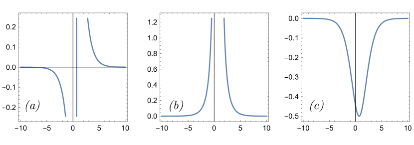
Figure 1: A solution of the mKdV hierarchy and its corresponding solutions in the KdV hierarchy via the Miura transformations (2.5). (a) We plot $\mathpzc{V}$ given by (5.22) against $\xi$. This is the equivalent of a 1-soliton solution, but does not have the usual soliton profile. (b) The corresponding solution of the KdV hierarchy obtained from (2.5) with minus sign. This is a peakon, which diverges at the mode. (c) A different solution of the KdV hierarchy is obtained from (2.5) with plus sign. This is a dark soliton over a zero vacuum background.

The zero vacuum 1-soliton solution of the mKdV hierarchy can be constructed from this approach yielding [56]

$$\mathpzc{V}=\partial_{x}\log\left(\dfrac{\tau_{1}}{\tau_{2}}\right),\qquad\tau_{1}=1-\dfrac{1}{2}e^{\xi},\qquad\tau_{2}=1+\dfrac{1}{2}e^{\xi},$$ (5.22)

where $\xi$ encodes the dispersion relation of each model within the hierarchy:

$$\xi(x,t_{N})=2\kappa x+2\kappa^{N}t_{N}\qquad(N=\pm 1,\pm 3,\dotsc).$$ (5.23)

Recall that only odd flows of the mKdV hierarchy admit zero vacuum. A plot of (5.22) against $\xi$ is shown fig. 1a. Note that $\mathpzc{V}\to 0$ as $|x|\to\infty$. Interestingly, starting from a single solution of the mKdV hierarchy, the Miura transformations (2.5) induce two types of solution of the KdV hierarchy, one for each sign. In fig. 1b we have a so-called peakon, which is discontinuous and diverges at the mode, while in fig. 1c we have a dark soliton. Thus, all models within the KdV hierarchy have both peakon and dark solitons; they are inherited from the same solution to the odd models of the mKdV hierarchy. The only difference among them is the change in the dispersion relation (5.23) which essentially changes the propagating speed of such localized waves. It is also possible to obtain $n$-dark-soliton and $n$-peakon solutions from the more general solutions of [56].

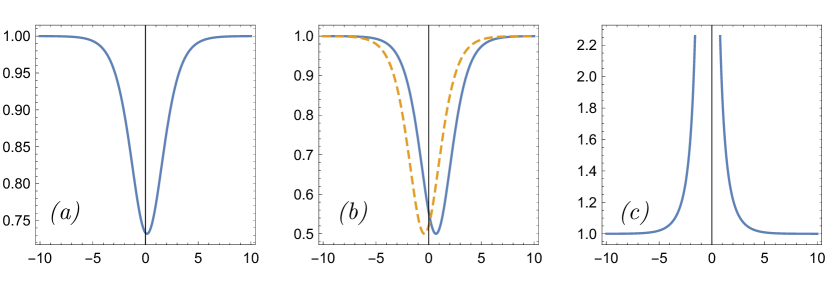
Figure 2: (a) Dark soliton of the mKdV hierarchy (5.24); we set $\mathpzc{V}_{0}=1$ and $\kappa=1/2$. (b) Using the two Miura transformations (2.5) we have dark solitons of the KdV hierarchy; the solid blue line is with plus sign and the dashed orange line with minus sign. (c) Shifting $\mathpzc{V}_{0}\to-\mathpzc{V}_{0}$ yields a peakon of the KdV hierarchy but now over a nonzero background $\mathcal{J}_{0}=\mathpzc{V}_{0}^{2}$.

A nonzero vacuum $\mathpzc{V}_{0}$ plays the role of a deformation parameter in comparison to the affine parameter of the algebra. Based on deformed vertex operators [56], the dispersion relations are obtained from eq. (5.21) and the nonzero vacuum 1-soliton of the mKdV hierarchy reads

$$\mathpzc{V}=\mathpzc{V}_{0}+\partial_{x}\log\left(\dfrac{\tau_{1}}{\tau_{2}}\right),\qquad\tau_{1}=1+\dfrac{\mathpzc{V}_{0}-\kappa}{2\kappa}e^{\xi},\qquad\tau_{2}=1+\dfrac{\mathpzc{V}_{0}+\kappa}{2\kappa}e^{\xi},$$ (5.24)

where the dispersion relation couples $\mathpzc{V}_{0}$ and $\kappa$, e.g., for the negative even flows we have

$$\xi(x,t_{-2n})=2\kappa x+\dfrac{2\kappa}{\mathpzc{V}_{0}(\kappa^{2}-\mathpzc{V}_{0}^{2})^{n}}t_{-2n},$$ (5.25)

while for the positive part of the hierarchy each dispersion relation needs to be computed from the respective gauge potential $A^{\text{mKdV}}_{t_{N},\text{vac}}$. A plot of the solution (5.24) against $\xi$ is shown in fig. 2a. Note that now we have a dark soliton of the mKdV hierarchy over the constant vacuum $\mathpzc{V}\to\mathpzc{V}_{0}$ as $|x|\to\infty$. When we replace this solution into the Miura transformations (2.5), both signs yield the same type of solution of the KdV hierarchy — with just a position shift — as illustrated in fig. 2b. These are again dark solitons but now for the KdV hierarchy, with a vacuum $\mathcal{J}_{0}=\mathpzc{V}_{0}^{2}$. Making $\mathpzc{V}_{0}\to-\mathpzc{V}_{0}<0$ the solution of the KdV hierarchy becomes a peakon over a nonzero background $\mathcal{J}_{0}=\mathpzc{V}_{0}^{2}$, as shown in fig. 2c. Similarly, $n$-dark-soliton or $n$-peakon solutions over a nontrivial vacuum can be obtained by plugging in the more general solutions proposed in [56] into the Miura transformations.

Peakons were proposed in the seminal paper [64] through the Camassa-Holm equation, and later noted to appear in other integrable models [65]. Dark solitons constitute an interesting and active research topic, with concrete experimental observation in Bose-Einstein condensates, nonlinear optics, and condensed matter physics [66, 67, 68, 69, 70, 71]. The above results show that both kinds of solutions are admissible among the models of the KdV hierarchy, including the KdV equation itself and its first negative flow (4.4). These two different solutions are obtained from the two possible Miura transformations leveraging the same solution of the mKdV hierarchy. We believe these facts have not been previously noticed in the literature.

6 Heisenberg subalgebras and commuting flows

We have considered individual flows — differential equations — of the mKdV and KdV hierarchies. However, an integrable hierarchy must have an infinite number of mutually commuting flows, which are related to an infinite number of involutive conserved charges. For a zero vacuum configuration of the mKdV hierarchy this is a consequence of the gauge potentials having the form $A_{t_{N},\text{vac}}^{\text{mKdV}}=E^{(n)}$ for $N=2n+1$, implying that the operators $A_{t_{N},\text{vac}}^{\text{mKdV}}$ are in the kernel of $E$ so they form an abelian subalgebra up to a central term, i.e., a Heisenberg subalgebra [23]. An important question that we now address is whether this remains true for a nonzero vacuum configuration and in particular for the negative even flows of the mKdV hierarchy.

Let us first recall some known facts. Denote the Lax operators of a generic integrable hierarchy by

$$\mathcal{L}_{N}\equiv\partial_{t_{N}}+A_{t_{N}},$$ (6.1)

where $\{t_{N}\}$ are the admissible time flows (with $t_{1}=x$). To show that any two given flows commute, $\left[\partial_{t_{N}},\partial_{t_{M}}\right]\mathcal{L}_{1}$, it is sufficient to show that $\left[\mathcal{L}_{N},\mathcal{L}_{M}\right]=0$; see, e.g., [22, 72]. For a general field configuration the Lax operators (6.1) are related to their values at some vacuum via the action of a dressing operator $\Theta$ [72], namely

$$\mathcal{L}_{N}=\Theta\mathcal{L}_{N,\text{vac}}\Theta^{-1}.$$ (6.2)

Therefore

$$\left[\mathcal{L}_{N},\mathcal{L}_{M}\right]=\Theta\left[\mathcal{L}_{N,\text{vac}},\mathcal{L}_{M,\text{vac}}\right]\Theta^{-1}$$ (6.3)

and one only needs to show commutation relations at the vacuum, $\big{[}\mathcal{L}_{N,\text{vac}},\mathcal{L}_{M,\text{vac}}\big{]}=0$. Thus, the infinite set of mutually commuting flows of an integrable hierarchy, obeying zero curvature equations (6.3), is defined with respect to some vacuum. Next, we discuss the two relevant cases of interest for the purposes of this paper and show that the mKdV hierarchy can be seen as two “distinct” hierarchies depending whether one uses zero or nonzero vacuum.

6.1 Zero vacuum and Type-I mKdV hierarchy

Let us recall the zero vacuum case $\mathpzc{V}\to\mathpzc{V}_{0}=0$, which is well-known [23]. For $N=2n+1$ and $M=2m+1$ being positive odd or negative odd we have the Lax operators at the vacuum given by

$$\mathcal{L}_{N,\text{vac}}^{\text{mKdV-I}}=\partial_{t_{N}}+E^{(N)},$$ (6.4)

where

$$E^{(N)}\equiv E^{(n)}_{\alpha}+E^{(n+1)}_{-\alpha}=\lambda^{n}\left(E_{\alpha}^{(0)}+E_{-\alpha}^{(1)}\right)\equiv\lambda^{n}E.$$ (6.5)

Note that $E^{(N)}\in\mathcal{K}_{E}$ which only admits odd-graded elements (A.14). These operators indeed form an abelian subalgebra

$$\left[E^{(N)},E^{(M)}\right]=0,$$ (6.6)

from which it follows that $\big{[}\mathcal{L}_{N,\text{vac}}^{\text{mKdV-I}},\mathcal{L}_{M,\text{vac}}^{\text{mKdV-I}}\big{]}=0$. Thus, the zero vacuum configuration defines an infinite set of mutually commuting flows indexed by $N,M$ positive or negative odd. They form the standard mKdV hierarchy, now referred to as mKdV Type-I for clarity.

Let $\Theta=\Theta_{I}$ be a dressing operator in eq. (6.2) for such a zero vacuum configuration. The gauge-Miura operator $S$ in eq. (2.3) maps the Type-I mKdV hierarchy into the KdV hierarchy, thus

$$\begin{split}\left[\mathcal{L}_{N}^{\text{KdV}},\mathcal{L}_{M}^{\text{KdV}}\right]&=S\left[\mathcal{L}_{N}^{\text{mKdV-I}},\mathcal{L}_{M}^{\text{mKdV-I}}\right]S^{-1}\\ &=\big{(}S\Theta_{I}\big{)}\left[\mathcal{L}_{N,\text{vac}}^{\text{mKdV-I}},\mathcal{L}_{M,\text{vac}}^{\text{mKdV-I}}\right]\big{(}S\Theta_{I}\big{)}^{-1}\\ &=0,\end{split}$$ (6.7)

showing that the flows of the KdV hierarchy in the orbit of such a zero vacuum commute.

6.2 Nonzero vacuum and Type-II mKdV hierarchy

We now consider a constant, nonzero, vacuum $\mathpzc{V}\to\mathpzc{V}_{0}\neq 0$. By careful inspection of the Lax operators defining the equations of motion of the mKdV hierarchy from Secs. 2 and 3 we conclude that they have the form

$$\mathcal{L}^{\text{mKdV-II}}_{1,\text{vac}} =\partial_{x}+\mathfrak{B},$$ (6.8a)

$$\mathcal{L}_{-2n,\text{vac}}^{\text{mKdV-II}} =\partial_{t_{-2n}}+(\mathpzc{V}_{0})^{-1}\mathfrak{B}^{(-2n+1)},$$ (6.8b)

$$\mathcal{L}_{2n+1,\text{vac}}^{\text{mKdV-II}} =\partial_{t_{2n+1}}+\sum_{j=1}^{n}c_{j}\mathpzc{V}_{0}^{2n-2j}\mathfrak{B}^{(2j+1)},$$ (6.8c)

for some numbers $c_{j}$ in (6.8c) and where ($N=2n+1$, $n=0,\pm 1,\dotsc$)

$$\mathfrak{B}^{(N)}\equiv E^{(N)}+\mathpzc{V}_{0}h^{(n)}=\lambda^{n}(E+\mathpzc{V}_{0}h)\equiv\lambda^{n}\mathfrak{B}.$$ (6.9)

Note that $\mathfrak{B}$ contains the vacuum $\mathpzc{V}_{0}$ as a parameter. The term $E^{(N)}$ has degree $2n+1$ and $h^{(n)}$ has degree $2n$ according to the principal gradation $\widehat{Q}\equiv 2\widehat{d}+\tfrac{1}{2}h^{(0)}$. If we associate degree $1$ to $\mathpzc{V}_{0}$, i.e., if we redefine the grading operator as $\widetilde{Q}\equiv\widehat{Q}+\widetilde{d}$, where $\widetilde{d}\equiv\mathpzc{V}_{0}\tfrac{\partial}{\partial\mathpzc{V}_{0}}$, then $\mathfrak{B}^{(N)}$ has degree $2n+1$ and it is a sum of two homogeneous terms of degree $2n+1$. Thus $\mathpzc{V}_{0}$ can be interpreted as a new spectral parameter defining a two-loop algebra as discussed in [73, 74]. Each individual term in the sum (6.8c) has degree $2n+1$, which is also the highest degree of the operator $\mathcal{L}_{2n+1}^{\text{mKdV}}$. Similarly, the operator (6.8b) has degree $-2n$, which is the lowest degree of operator $\mathcal{L}_{-2n}^{\text{mKdV}}$. From (6.9) we again have an abelian subalgebra,

$$\left[\mathfrak{B}^{(N)},\mathfrak{B}^{(M)}\right]=0,$$ (6.10)

in close analogy with the zero vacuum case (6.6). This implies that for $N,M$ indexed as in eqs. (6.8), i.e., positive odd or negative even, $\big{[}\mathcal{L}_{N,\text{vac}}^{\text{mKdV-II}},\mathcal{L}_{M,\text{vac}}^{\text{mKdV-II}}\big{]}=0$. By the dressing transformation (6.3) with a suitable operator $\Theta=\Theta_{II}$, we have $\big{[}\mathcal{L}_{N}^{\text{mKdV-II}},\mathcal{L}_{M}^{\text{mKdV-II}}\big{]}=0$ for a general field configuration in the orbit of such a nonzero vacuum — which is parametrized by $\mathpzc{V}_{0}$. Therefore, such mutually commuting flows define a proper integrable hierarchy, which we refer to as mKdV Type-II. We provide an explicit example of such commuting flows in sec. C in the appendix.

Thus, the mKdV-II hierarchy has positive odd and negative even flows that commute among themselves. The gauge-Miura transformation (5.2) and (5.5) also maps the mKdV-II hierarchy into the KdV hierarchy. More precisely, under the dressing transformation (6.2) we now have

$$\begin{split}\left[\mathcal{L}_{\lceil N\rceil}^{\text{KdV}},\mathcal{L}_{\lceil M\rceil}^{\text{KdV}}\right]&=S\left[\mathcal{L}_{N}^{\text{mKdV-II}},\mathcal{L}_{M}^{\text{mKdV-II}}\right]S^{-1}\\ &=\big{(}S\Theta_{II}\big{)}\left[\mathcal{L}_{N,\text{vac}}^{\text{mKdV-II}},\mathcal{L}_{M,\text{vac}}^{\text{mKdV-II}}\right]\big{(}S\Theta_{II}\big{)}^{-1}\\ &=0,\end{split}$$ (6.11)

showing that the flows of the KdV hierarchy in the orbit of such a nonzero vacuum — parametrized by $\mathcal{J}_{0}=\mathpzc{V}_{0}^{2}$ — also commute. For consistency of notation, above we defined $\lceil N\rceil\equiv N$ for $N=2n+1$ (positive odd) and $\lceil N\rceil\equiv-2n+1$ for $N=-2n$ (negative even).

By analogous reason that the operators (6.4) only admit odd flows, the operators (6.8) only admit negative even flows, besides the positive odd ones. The reason is the following. For negative even flows ($N=-2n$), $A_{t_{N},\text{vac}}^{\text{mKdV}}=\big{(}D^{(-2n)}_{\text{vac}}+D^{(-2n+1)}_{\text{vac}}\big{)}+\dotsm+\big{(}D^{(-2)}_{\text{vac}}+D^{(-1)}_{\text{vac}}\big{)}$, where each term in parenthesis combines precisely into a term proportional to $\mathfrak{B}^{(j)}$, i.e., $D^{(2j)}_{\text{vac}}+D^{(2j-1)}_{\text{vac}}\sim\mathfrak{B}^{(j)}$ — actually, only the first term survives yielding the form (6.8b). The same structure repeats itself for positive odd flows ($N=2n+1$), namely $A_{t_{N},\text{vac}}^{\text{mKdV}}=\big{(}D^{(2n+1)}_{\text{vac}}+D^{(2n)}_{\text{vac}}\big{)}+\dotsm+\big{(}D^{(1)}_{\text{vac}}+D^{(0)}_{\text{vac}}\big{)}$ — here all terms survive yielding the form (6.8c). However, for negative odd flows ($N=-2n+1$) $A_{t_{N},\text{vac}}^{\text{mKdV}}=D^{(-2n+1)}_{\text{vac}}+\dotsm+D^{(-1)}_{\text{vac}}$ contains an odd number of terms and therefore can never combine into a sum of $\mathfrak{B}^{(j)}$’s alone. Therefore:

• The mKdV-I hierarchy has positive odd and negative odd flows, and is defined in the orbit of a zero vacuum ($\mathpzc{V}_{0}=0$);

• The mKdV-II hierarchy has negative even and positive odd flows, and is defined in the orbit of a nonzero vacuum (parametrized by $\mathpzc{V}_{0}\neq 0$);

• Notably, the differential equations for the negative parts of mKdV-I and mKdV-II are different. However, both mKdV-I and mKdV-II have the same differential equations for their positive parts. Such positive flow equations therefore allow both types of solution, i.e., with zero (mKdV-I) and nonzero (mKdV-II) vacuum.

• The flows within each mKdV-I and mKdV-II commute among themselves, but crossed flows between them do not. That is, only flows defined in the orbit of the same vacuum commute.

Furthermore, the same gauge-Miura transformation $S$ maps both mKdV-I and mKdV-II into the KdV hierarchy that has only odd flows (positive and negative); see eqs. (6.7) and (6.11). This explains why the entire KdV hierarchy admits both types of solution, i.e., with zero and nonzero vacuum. In light of this discussion, the diagrams (2.17) and (5.7) should be seen as a shorthand for

      and       (6.12)

where $N$ is positive or negative odd, and $M$ is positive odd or negative even. Note also that commuting flows of the KdV hierarchy are defined in the orbit of some vacuum, defined by the mappings (6.7) and (6.11). However, contrary to mKdV, the differential equations in the KdV hierarchy are the same in both situations.

7 Extension to $\widehat{s\ell}(3)$

The previous ideas generalize to more complex cases such as integrable models constructed from $\widehat{s\ell}(3)$ or more generally from $\widehat{s\ell}(r+1)$; see the appendix A for definitions. Let us consider explicitly the $\widehat{s\ell}(3)$ case first. The analog of the mKdV gauge potential (2.1) has now two fields, $\mathpzc{V}_{1}(x,t_{N})$ and $\mathpzc{V}_{2}(x,t_{N})$, and assumes the form

$$A_{x}^{\text{mKdV}}=E+A_{0}=E_{\alpha_{1}}^{(0)}+E_{\alpha_{2}}^{(0)}+E_{-\alpha_{1}-\alpha_{2}}^{(1)}+\mathpzc{V}_{1}h_{1}^{(0)}+\mathpzc{V}_{2}h_{2}^{(0)}.$$ (7.1)

Similarly, the KdV gauge potential (2.2) acquires two fields, $\mathcal{J}_{1}(x,t_{N})$ and $\mathcal{J}_{2}(x,t_{N})$, where one of them is with $A_{-1}\in{\cal G}_{-1}$ and the other is with $A_{-2}\in{\cal G}_{-2}$,

$$A_{x}^{\text{KdV}}=E+A_{-1}+A_{-2}=E_{\alpha_{1}}^{(0)}+E_{\alpha_{2}}^{(0)}+E_{-\alpha_{1}-\alpha_{2}}^{(1)}+\mathcal{J}_{1}E_{-\alpha_{1}}^{(0)}+\mathcal{J}_{2}E_{-\alpha_{1}-\alpha_{2}}^{(0)}.$$ (7.2)

Instead of two gauge-Miura transformations (2.3) now there are three, $S\in\{S_{1},S_{2},S_{3}\}$, all leading to the same correspondence (see [55] for details). We show results for one of them for simplicity, namely

$$A_{x}^{\text{KdV}}=S_{1}A_{x}^{\text{mKdV}}S_{1}^{-1}+S_{1}\partial_{x}S_{1}^{-1},$$ (7.3)

where

$$S_{1}=e^{\gamma_{3}E_{-\alpha_{1}-\alpha_{2}}^{(0)}}e^{\gamma_{2}E_{-\alpha_{2}}^{(0)}}e^{\gamma_{1}E_{-\alpha_{1}}^{(0)}}=\begin{pmatrix}1&0&0\\ \partial_{x}\phi_{1}&1&0\\ (\partial_{x}\phi_{1})^{2}-\partial_{x}^{2}\phi_{1}&\partial_{x}\phi_{2}&1\\ \end{pmatrix},$$ (7.4)

$\mathpzc{V}_{1}\equiv\partial_{x}\phi_{1}$, $\mathpzc{V}_{2}\equiv\partial_{x}\phi_{2}$, $\gamma_{1}=\partial_{x}\phi_{1}$, $\gamma_{2}=\partial_{x}\phi_{2}$, and $\gamma_{3}=(\partial_{x}\phi_{1})^{2}-(\partial_{x}\phi_{1})(\partial_{x}\phi_{2})-\partial_{x}^{2}\phi_{1}$. Such a gauge transformation realizes a Miura-type transformation among the fields:

$$\mathcal{J}_{1} =-\partial_{x}\mathpzc{V}_{1}-\partial_{x}\mathpzc{V}_{2}+\mathpzc{V}_{1}^{2}-\mathpzc{V}_{1}\mathpzc{V}_{2}+\mathpzc{V}_{2}^{2},$$ (7.5a)

$$\mathcal{J}_{2} =-2\mathpzc{V}_{1}\partial_{x}\mathpzc{V}_{1}+\mathpzc{V}_{1}\partial_{x}\mathpzc{V}_{2}+\partial_{x}^{2}\mathpzc{V}_{1}+\mathpzc{V}_{1}^{2}\mathpzc{V}_{2}-\mathpzc{V}_{1}\mathpzc{V}_{2}^{2}.$$ (7.5b)

As before, such a gauge transformation provides a 1-to-1 correspondence between the models of the positive part of these hierarchies. However, the negative part is more subtle and now a triple of temporal mKdV gauge potentials, $A_{t_{-3n+2}}^{\text{mKdV}}$, $A_{t_{-3n+1}}^{\text{mKdV}}$ and $A_{t_{-3n}}^{\text{mKdV}}$, fuse into a single temporal KdV gauge potential, $A_{t_{-3n+2}}^{\text{KdV}}$, as summarized by the diagram

(7.6)

For the positive part the index $N$ can assume values $3n+1$ or $3n+2$, for $n=0,1,\dotsc$. This is because the highest grade component of the zero curvature condition, $\big{[}E,\mathcal{D}^{(N)}_{N}\big{]}=0$, implies that $\mathcal{D}^{N}_{N}\in\mathcal{K}_{E}$, which from eq. (A.18) there are two possibilities, each leading to a different model. However, for the negative part we have $-N=3n+2$, for $n=-1,-2,\dotsc$.

The derivation of the equations of motion from the zero curvature condition, and the explicit gauge transformation for the temporal gauge potentials, follow exactly the same procedure as previously explained for $\widehat{s\ell}(2)$ although the calculations are longer. We thus limit the discussion to stating the main results for the sake of simplicity. Some of the representative models within these hierarchies, related by the above diagram, are described as follows.

• $t_{1}$-flow  This case gives the chiral wave equations $\partial_{t_{1}}\mathpzc{V}_{1}=\partial_{x}\mathpzc{V}_{1}$ and $\partial_{t_{1}}\mathpzc{V}_{2}=\partial_{x}\mathpzc{V}_{2}$ for the 2-component mKdV, and similar equations for the 2-component KdV.

• $t_{2}$-flow  For the $\widehat{s\ell}(3)$-mKdV hierarchy we have the equations of motion

  $$3\partial_{t_{2}}\mathpzc{V}_{1} =\partial_{x}\left(\mathpzc{V}_{1}^{2}+2\mathpzc{V}_{1}\mathpzc{V}_{2}-2\mathpzc{V}_{2}^{2}-\partial_{x}\mathpzc{V}_{1}+2\partial_{x}\mathpzc{V}_{2}\right),$$ (7.7a)

  $$3\partial_{t_{2}}\mathpzc{V}_{2} =\partial_{x}\left(2\mathpzc{V}_{1}^{2}-2\mathpzc{V}_{1}\mathpzc{V}_{2}-\mathpzc{V}_{2}^{2}-2\partial_{x}\mathpzc{V}_{1}+\partial_{x}\mathpzc{V}_{2}\right).$$ (7.7b)

  Its counterpart in the $\widehat{s\ell}(3)$-KdV hierarchy is given by

  $$\partial_{t_{2}}\mathcal{J}_{1} =\partial_{x}\left(2\mathcal{J}_{2}+\partial_{x}\mathcal{J}_{1}\right),$$ (7.8a)

  $$3\partial_{t_{2}}\mathcal{J}_{2} =\partial_{x}\left(\mathcal{J}_{1}^{2}-3\partial_{x}\mathcal{J}_{2}-2\partial_{x}^{2}\mathcal{J}_{1}\right).$$ (7.8b)

• $t_{-1}$-flow (mKdV)  The $\widehat{s\ell}(3)$-mKdV hierarchy yields an affine Toda field theory as the first negative flow given by

  $$\partial_{t_{-1}}\partial_{x}\phi_{1} =e^{2\phi_{1}-\phi_{2}}-e^{-\phi_{1}-\phi_{2}},$$ (7.9a)

  $$\partial_{t_{-1}}\partial_{x}\phi_{2} =e^{-\phi_{1}+2\phi_{2}}-e^{-\phi_{1}-\phi_{2}},$$ (7.9b)

  where $\mathpzc{V}_{1}\equiv\partial_{x}\phi_{1}$ and $\mathpzc{V}_{2}\equiv\partial_{x}\phi_{2}$.

• $t_{-2}$-flow (mKdV) We have the integro-differential equations

  $$\partial_{t_{-2}}\partial_{x}\phi_{1} =e^{2\phi_{1}-\phi_{2}}\partial_{x}^{-1}\left[e^{-\phi_{1}-\phi_{2}}-e^{-\phi_{1}+2\phi_{2}}\right]$$

  $$-e^{-\phi_{1}-\phi_{2}}\partial_{x}^{-1}\left[e^{-\phi_{1}+2\phi_{2}}-e^{2\phi_{1}-\phi_{2}}\right],$$ (7.10a)

  $$\partial_{t_{-2}}\partial_{x}\phi_{2} =-e^{-\phi_{1}+2\phi_{2}}\partial_{x}^{-1}\left[e^{-\phi_{1}-\phi_{2}}-e^{2\phi_{1}-\phi_{2}}\right]$$

  $$-e^{-\phi_{1}-\phi_{2}}\partial_{x}^{-1}\left[e^{-\phi_{1}+2\phi_{2}}-e^{2\phi_{1}-\phi_{2}}\right].$$ (7.10b)

• $t_{-3}$-flow (mKdV) In this case we obtain

  $$\partial_{t_{-3}}\partial_{x}\phi_{1} =e^{\phi_{1}-\phi_{2}}\partial_{x}^{-1}\left[e^{2\phi_{1}-\phi_{2}}\partial_{x}^{-1}e^{-\phi_{1}+2\phi_{2}}\right]$$

  $$-e^{\phi_{1}-\phi_{2}}\partial_{x}^{-1}\left[e^{-\phi_{1}+2\phi_{2}}\partial_{x}^{-1}e^{2\phi_{1}-\phi_{2}}\right]$$

  $$+2e^{2\phi_{1}-\phi_{2}}\partial_{x}^{-1}\left[e^{-\phi_{1}+2\phi_{2}}\partial_{x}^{-1}e^{-\phi_{1}-\phi_{2}}\right]$$

  $$+e^{2\phi_{1}-\phi_{2}}\partial_{x}^{-1}\left[e^{-\phi_{1}-\phi_{2}}\partial_{x}^{-1}e^{-\phi_{1}+2\phi_{2}}\right],$$ (7.11a)

  $$\partial_{t_{-3}}\partial_{x}\phi_{2} =-e^{\phi_{1}-\phi_{2}}\partial_{x}^{-1}\left[e^{-\phi_{1}+2\phi_{2}}\partial_{x}^{-1}e^{2\phi_{1}-\phi_{2}}\right]$$

  $$+e^{\phi_{1}-\phi_{2}}\partial_{x}^{-1}\left[e^{2\phi_{1}-\phi_{2}}\partial_{x}^{-1}e^{-\phi_{1}+2\phi_{2}}\right]$$

  $$-2e^{-\phi_{1}+2\phi_{2}}\partial_{x}^{-1}\left[e^{2\phi_{1}-\phi_{2}}\partial_{x}^{-1}e^{\phi_{1}-\phi_{2}}\right]$$

  $$-e^{-\phi_{1}+2\phi_{2}}\partial_{x}^{-1}\left[e^{-\phi_{1}-\phi_{2}}\partial_{x}^{-1}e^{2\phi_{1}-\phi_{2}}\right].$$ (7.11b)

• $t_{-1}$-flow (KdV) For the first negative flow of the $\widehat{s\ell}(3)$-KdV hierarchy we obtain

  $$0 =2\partial_{t_{-1}}\partial_{x}\eta_{1}\,(\partial_{x}\eta_{1})^{2}+2\partial_{t_{-1}}\eta_{1}\,\partial_{x}^{2}\eta_{1}\,\partial_{x}\eta_{1}-4\partial_{t_{-1}}\partial_{x}^{3}\eta_{1}\,\partial_{x}\eta_{1}$$

  $$-3\partial_{t_{-1}}\partial_{x}^{2}\eta_{2}\,\partial_{x}\eta_{1}-6\partial_{x}^{2}\eta_{1}\,\partial_{t_{-1}}\partial_{x}^{2}\eta_{1}-6\partial_{t_{-1}}\partial_{x}\eta_{1}\,\partial_{x}^{3}\eta_{1}-2\partial_{t_{-1}}\eta_{1}\,\partial_{x}^{4}\eta_{1}$$

  $$+2\partial_{t_{-1}}\partial_{x}^{5}\eta_{1}+9\partial_{x}\eta_{2}\,\partial_{t_{-1}}\partial_{x}\eta_{2}-6\partial_{t_{-1}}\partial_{x}\eta_{1}\,\partial_{x}^{2}\eta_{2}+3\partial_{t_{-1}}\eta_{2}\,\partial_{x}^{2}\eta_{2}$$

  $$-3\partial_{t_{-1}}\eta_{1}\,\partial_{x}^{3}\eta_{2}+3\partial_{t_{-1}}\partial_{x}^{4}\eta_{2},$$ (7.12a)

  $$0 =2\partial_{t_{-1}}\partial_{x}\eta_{1}\,\partial_{x}^{2}\eta_{1}+\partial_{t_{-1}}\eta_{2}\,\partial_{x}^{2}\eta_{1}+\partial_{x}\eta_{1}\,\partial_{t_{-1}}\partial_{x}^{2}\eta_{1}+\partial_{t_{-1}}\eta_{1}\,\partial_{x}^{3}\eta_{1}$$

  $$-\partial_{t_{-1}}\partial_{x}^{4}\eta_{1}+3\partial_{t_{-1}}\partial_{x}\eta_{1}\,\partial_{x}\eta_{2}+2\partial_{x}\eta_{1}\,\partial_{t_{-1}}\partial_{x}\eta_{2}$$

  $$+2\partial_{t_{-1}}\eta_{1}\,\partial_{x}^{2}\eta_{2}-2\partial_{t_{-1}}\partial_{x}^{3}\eta_{2},$$ (7.12b)

  where $\mathcal{J}_{1}\equiv\partial_{x}\eta_{1}$ and $\mathcal{J}_{2}\equiv\partial_{x}\eta_{2}$. The above model corresponds to the counterpart of the affine Toda field theory (7.9) in the $\widehat{s\ell}(3)$-KdV hierarchy. Actually, all three mKdV models (7.9), (7.10) and (7.11) are connected to model (7.12) by gauge transformation; see diagram (7.6).

• Higher positive flows, or lower negative ones, for both hierarchies can be obtained as well, although the equations quickly become quite complicated.

For the affine Toda model (7.9) we have, besides the Miura-type transformation (7.5), the “temporal Miura relations”

$$\partial_{t_{-1}}\eta_{1}=3e^{-\phi_{1}-\phi_{2}},\qquad\partial_{t_{-1}}\eta_{2}=3(\partial_{x}\phi_{1})e^{-\phi_{1}-\phi_{2}},$$ (7.13)

which are the analog of relation (5.12) for sinh-Gordon. The map between models (7.10) and (7.12) involve instead the relations

$$\partial_{t_{-1}}\eta_{1} =3e^{-\phi_{1}-\phi_{2}}\partial_{x}^{-1}\left(e^{-\phi_{1}+2\phi_{2}}-e^{2\phi_{1}-\phi_{2}}\right),$$ (7.14a)

$$\partial_{t_{-1}}\eta_{2} =3e^{\phi_{1}-2\phi_{2}}+3e^{-\phi_{1}-\phi_{2}}(\partial_{x}\phi_{1})\partial_{x}^{-1}\left(e^{-\phi_{1}+2\phi_{2}}-e^{2\phi_{1}-\phi_{2}}\right),$$ (7.14b)

and in the case of model (7.11) we have

$$\partial_{t_{-1}}\eta_{1} =3e^{-\phi_{1}-\phi_{2}}\partial_{x}^{-1}\left(e^{-\phi_{1}+2\phi_{2}}\partial_{x}^{-1}e^{2\phi_{1}-\phi_{2}}-e^{2\phi_{1}-\phi_{2}}\partial_{x}^{-1}e^{-\phi_{1}+2\phi_{2}}\right),$$ (7.15a)

$$\partial_{t_{-1}}\eta_{2} =3e^{\phi_{1}-2\phi_{2}}\partial_{x}^{-1}e^{-\phi_{1}+2\phi_{2}}$$

$$+3(\partial_{x}\phi_{1})e^{-\phi_{1}-\phi_{2}}\partial_{x}^{-1}\left[e^{-\phi_{1}+2\phi_{2}}\partial_{x}^{-1}e^{2\phi_{1}-\phi_{2}}-e^{2\phi_{1}-\phi_{2}}\partial_{x}^{-1}e^{-\phi_{1}+2\phi_{2}}\right].$$ (7.15b)

Such relations follow immediately from the zero curvature construction and the gauge-Miura transformations; they would otherwise be impossible to guess, i.e., based on the equations of motion and the Miura transformation (7.5) alone.

The vacuum structure for the negative flows follow a similar structure as the previous $\widehat{s\ell}(2)$ case, and will be discussed in more generality in sec. 8.

7.1 Tzitzéica-Bullough-Dodd and its KdV counterpart

As a particular case of the affine Toda theory (7.9), setting $\phi_{1}=\phi_{2}=-\varphi$ we obtain the Tzitzéica-Bullough-Dodd model in light cone coordinates:

$$\partial_{t_{-1}}\partial_{x}\varphi=e^{2\varphi}-e^{-\varphi}.$$ (7.16)

Form factors of this model were obtained in [75], and its relation with the Izergin-Korepin massive quantum field theory through Bethe ansatz equations was demonstrated in [76], as well as its conformal limit. Under this reduction, the Miura transformation (7.5) implies

$$\mathcal{J}_{1} \equiv\partial_{x}\eta=(\partial_{x}\varphi)^{2}+2\partial_{x}^{2}\varphi,$$ (7.17a)

$$\mathcal{J}_{2} \equiv\partial_{x}\eta_{2}=-\tfrac{1}{2}\partial_{x}^{2}\eta,$$ (7.17b)

so that system (7.12) reduces to

$$\begin{split}2&\partial_{t_{-1}}\partial_{x}^{5}\eta+8\big{(}\partial_{t_{-1}}\partial_{x}\eta_{1}\big{)}\big{(}\partial_{x}\eta\big{)}^{2}+2\big{(}4\partial_{t_{-1}}\eta\,\partial_{x}^{2}\eta-5\partial_{t_{-1}}\partial_{x}^{3}\eta\big{)}\big{(}\partial_{x}\eta\big{)}\\ &\qquad-15\partial_{x}^{2}\eta\,\partial_{t_{-1}}\partial_{x}^{2}\eta-9\partial_{t_{-1}}\partial_{x}\eta\,\partial_{x}^{3}\eta-2\partial_{t_{-1}}\eta\,\partial_{x}^{4}\eta=0.\end{split}$$ (7.18)

Moreover, the temporal Miura relation (7.13) yields

$$\partial_{t_{-1}}\eta=3e^{2\varphi}.$$ (7.19)

The integrable model (7.18) corresponds to the KdV counterpart of the Tzitzéica-Bullough-Dodd (7.16), in the same way that the sinh-Gordon is related to the first negative KdV flow (4.4). Both sinh-Gordon and Tzitzéica-Bullough-Dood can be seen as (different) integrable perturbations of the conformal Liouville theory, which is obtained from Einsteins’s equations in 2D and has important connections in string theory [29].

7.2 Commuting flows

The same arguments used for $\widehat{s\ell}(2)$ — see sec. 6 — extend to $\widehat{s\ell}(3)$ as we now show. The spatial Lax operator is

$$\begin{split}\mathcal{L}_{1}^{\text{mKdV}}&=\partial_{x}+E+A_{0}\\ &=\partial_{x}+E_{\alpha_{1}}^{(0)}+E_{\alpha_{2}}^{(0)}+E_{-(\alpha_{1}+\alpha_{2})}^{(1)}+\mathpzc{V}_{1}h_{1}^{(0)}+\mathpzc{V}_{2}h_{2}^{(0)}.\end{split}$$ (7.20)

The kernel of $E$ (recall sec. A.3 in the appendix) has elements $\mathcal{K}_{E}=\{E^{(3n+1)},E^{(3n+2)}\}$ with

$$E^{(3n+1)} \equiv E_{\alpha_{1}}^{n}+E_{\alpha_{2}}^{(n)}+E_{-\alpha_{1}-\alpha_{2}}^{(n+1)}=\lambda^{n}E,$$ (7.21a)

$$E^{(3n+2)} \equiv E_{-\alpha_{1}}^{(n+1)}+E_{-\alpha_{2}}^{(n+1)}+E_{\alpha_{1}+\alpha_{2}}^{(n)}=\lambda^{n+1}E^{\dagger}.$$ (7.21b)

For zero vacuum configuration $\mathpzc{V}_{i}\to\mathpzc{V}_{i,0}=0$ ($i=1,2$) we have

$$\mathcal{L}^{\text{mKdV-I}}_{3n+1,\text{vac}} =\partial_{t_{3n+1}}+E^{(3n+1)},$$ (7.22a)

$$\mathcal{L}^{\text{mKdV-I}}_{3n+2,\text{vac}} =\partial_{t_{3n+2}}+E^{(3n+2)},$$ (7.22b)

for $n=0,\pm 1,\pm 2,\dotsc$. These include both the positive and negative flows that admit zero vacuum. As for the $\widehat{s\ell}(2)$ case (6.6), we also have an abelian subalgebra up to a central term:

$$\left[E^{(3n+p)},E^{(3m+p^{\prime})}\right]=0\qquad(p,p^{\prime}=1,2).$$ (7.23)

This implies commuting flows at the vacuum and, as a consequence of dressing transformations, also $\big{[}\mathcal{L}_{3n+p}^{\text{mKdV-I}},\mathcal{L}_{3m+p^{\prime}}^{\text{mKdV-I}}\big{]}=0$ for a general field configuration in its orbit. By gauge-Miura (7.3) this implies commuting flows of the KdV hierarchy, analogously to (6.7). Note, however, that the mapping is degenerate, i.e., there is a 2-fold mapping for the negative part of the hierarchies described in the diagram (7.6) regarding zero vacuum, i.e., this relation can be broken down into

      and       (7.24)

where $n=0,1,2,\dotsc$ (left diagram) accounts for positive flows and $m=1,2,\dotsc$ (right diagram) accounts for negative flows.

Moving on to the nonzero vacuum case $\mathpzc{V}_{i}\to\mathpzc{V}_{i,0}\neq 0$ ($i=1,2$), we have the Lax operator

$$\mathcal{L}_{1,\text{vac}}^{\text{mKdV-II}}=\partial_{x}+\mathfrak{B},\qquad\mathfrak{B}\equiv E+\mathpzc{V}_{1,0}h_{1}^{(0)}+\mathpzc{V}_{2,0}h_{2}^{(0)}.$$ (7.25)

It turns out that the element $\mathfrak{B}$ has a well-defined kernel

$$\mathcal{K}_{\mathfrak{B}}=\{\mathfrak{B}^{(3n+1)},\mathfrak{B}^{(3n+2)}\},$$ (7.26)

where

$$\mathfrak{B}^{(3n+1)} =E^{(3n+1)}+\mathpzc{V}_{1,0}h_{1}^{(n)}+\mathpzc{V}_{2,0}h_{2}^{(n)},$$ (7.27a)

$$\mathfrak{B}^{(3n+2)} =E^{(3n+2)}-\left(\mathpzc{V}_{1,0}+\mathpzc{V}_{2,0}\right)E_{\alpha_{2}}^{(n)}+\left(\mathpzc{V}_{1,0}-2\mathpzc{V}_{2,0}\right)E_{-(\alpha_{1}+\alpha_{2})}^{(n+1)}$$

$$+\frac{1}{3}\left(\mathpzc{V}_{1,0}+\mathpzc{V}_{2,0}\right)\left(\mathpzc{V}_{1,0}-2\mathpzc{V}_{2,0}\right)h_{1}^{(n)}+\frac{2}{3}\left(\mathpzc{V}_{1,0}+\mathpzc{V}_{2,0}\right)\left(\mathpzc{V}_{1,0}-2\mathpzc{V}_{2,0}\right)h_{2}^{(n)}.$$ (7.27b)

Similarly to (7.23), these elements form therefore an abelian subalgebra up to a central term:

$$\left[\mathfrak{B}^{(3n+p)},\mathfrak{B}^{(3m+p^{\prime})}\right]=0\qquad(p,p^{\prime}=1,2).$$ (7.28)

The Lax operators $\mathcal{L}_{N}^{\text{mKdV-II}}=\partial_{t_{N}}+A_{t_{N}}^{\text{mKdV-II}}$ admitting nonzero vacuum are indexed by positive flows $N=3n+p$, for $p=1,2$ and $n=0,1,2,\dotsc$, and by negative flows $N=-3n$, for $n=1,2,\dotsc$ — see sec. 8.4 below where we discuss this in more generality for $\widehat{s\ell}(r+1)$. Each of these Lax operators obey a zero curvature equation with $\mathcal{L}_{1}^{\text{mKdV}}$ by definition (this is how the individual differential equations were constructed to begin with). Therefore, setting the fields at the vacuum, $\mathpzc{V}_{i}\to\mathpzc{V}_{i,0}$, these Lax operators obey zero curvature equations with the operator $\mathcal{L}_{1,\text{vac}}^{\text{mKdV-II}}$ in eq. (7.25), i.e., $\big{[}\mathfrak{B},A_{t_{N,\text{vac}}}^{\text{mKdV-II}}\big{]}=0$. We conclude that $A_{t_{N},\text{vac}}^{\text{mKdV-II}}\in\mathcal{K}_{\mathfrak{B}}$ must be a linear combination of the operators in the abelian subalgebra (7.28) and hence commute among themselves. This shows that $\big{[}\mathcal{L}_{N,\text{vac}}^{\text{mKdV-II}},\mathcal{L}_{M,\text{vac}}^{\text{mKdV-II}}\big{]}=0$ for such flows, which is also true for a general field configuration in the orbit of this nonzero vacuum by the dressing action. Moreover, the gauge-Miura correspondence (7.3) then implies that the associated KdV flows in the orbit of a nonzero vacuum also commute. In this case the mapping is illustrated as ($n=0,1,\dotsc$, $m=1,2,\dotsc$)

      and       (7.29)

8 Extension to $\widehat{s\ell}(r+1)$

In light of the previous results we now lay out the extension for general affine Lie algebras $\widehat{s\ell}(r+1)$. In this case the spatial gauge potential of the multicomponent mKdV hierarchy is given by

$$A_{x}^{\text{mKdV}}=E+A_{0},$$ (8.1)

where

$$A_{0}=\mathpzc{V}_{1}h^{(0)}_{1}+\dotsm+\mathpzc{V}_{r}h^{(0)}_{r}\in{\cal G}_{0}$$ (8.2)

contains $r$ fields $\mathpzc{V}_{i}(x,t_{N})$ ($i=1,\dotsc,r$). Similarly, the spatial gauge potential of the multicomponent KdV hierarchy is

$$A_{x}^{\text{KdV}}=E+A_{-1}+\dotsm+A_{-r},$$ (8.3)

where

$$A_{-i}=\mathcal{J}_{i}\;E_{-(\alpha_{1}+\alpha_{2}+\dotsm+\alpha_{i})}^{(0)}\in{\cal G}_{-i}$$ (8.4)

contains the field $\mathcal{J}_{i}(x,t_{N})$ ($i=1,\dotsc,r$). Such hierarchies have positive and negative flow evolution equations as described below.

8.1 Positive flows

The positive part of the $\widehat{s\ell}(r+1)$-mKdV hierarchy has temporal gauge potential in the form

$$A_{t_{N}}^{\text{mKdV}}=D^{(N)}_{N}+D^{(N-1)}_{N}+\dotsm+D^{(0)}_{N},$$ (8.5)

while for the positive part of the $\widehat{s\ell}(r+1)$-KdV hierarchy we have the form

$$A_{t_{N}}^{\text{KdV}}=\mathcal{D}^{(N)}_{N}+\mathcal{D}^{(N-1)}_{N}+\dotsm+\mathcal{D}^{(-r+1)}_{N}+\mathcal{D}^{(-r)}_{N}.$$ (8.6)

Thus, the highest grade component of the zero curvature condition yields

$$\left[E,D^{(N)}_{N}\right]=0,\qquad\left[E,\mathcal{D}^{(N)}_{N}\right]=0,$$ (8.7)

$\partial_{x}D^{(N)}_{N}=0$, and $\partial_{x}\mathcal{D}^{(N)}_{N}=0$, implying that $N=(r+1)n+p$ for $n=0,1,\dotsc$ and $p=1,\dotsc,r$ for both hierarchies. This condition arises because $D^{(N)}_{N}$ and $\mathcal{D}^{(N)}_{N}$ must be in the kernel $\mathcal{K}_{E}$ defined in eq. (A.9).

8.2 Negative flows

The negative flows of the $\widehat{s\ell}(r+1)$-mKdV follows the structure

$$A_{t_{-N}}^{\text{mKdV}}=D^{(-N)}_{-N}+D^{(-N+1)}_{-N}+\dotsm+D^{(-1)}_{-N},$$ (8.8)

while for its KdV counterpart we propose

$$A_{t_{-N}}^{\text{KdV}}=\mathcal{D}^{(-N-2r)}_{-N}+\mathcal{D}^{(-N-2r+1)}_{-N}+\dotsm+\mathcal{D}^{(-1)}_{-N}.$$ (8.9)

From the zero curvature condition, the lowest grade component with gauge potential (8.8) implies no restriction on $N$, i.e., $D^{(-N)}_{-N}$ does not need to be in the kernel $\mathcal{K}_{E}$ and therefore can assume all negative integer values $-N=-1,-2,\dotsc$. However, for the KdV case with potential (8.9) we have the condition

$$\left[A_{-r},\mathcal{D}^{(-N-2r)}_{-N}\right]=0,$$ (8.10)

which together with consistency of the zero curvature condition requires that $-N=(r+1)n+r$ for $n=-1,-2,\dotsc$. This is because $\mathcal{D}^{(-N-2r)}_{-N}$ must proportional to the element $E_{-(\alpha_{1}+\dotsm+\alpha_{r})}^{(n+1)}\in{\cal G}_{(r+1)n+1}$ so that the zero curvature condition can be solved non trivially — here we again adopt the convention that the first negative flow is labelled as $t_{-1}$, which requires shifting $-N=(r+1)n+r$. Therefore, a “block” of $r+1$ models of the negative $\widehat{s\ell}(r+1)$-mKdV hierarchy maps into a single model of the $\widehat{s\ell}(r+1)$-KdV hierarchy via gauge-Miura transformations, as described in more detail below. We note also that the $t_{-1}$ mKdV flow corresponds to an affine Toda field theory which is thus related to the $t_{-1}$ KdV flow by gauge transformations.

8.3 Gauge-Miura maps

It has been shown that for $\widehat{s\ell}(r+1)$ the number of possible gauge-Miura transformations, $S_{j}$, is given by $r+1$ [55]. More specifically:

• We have the form $S_{j+1}=E^{(-j)}+s^{(-j-1)}+s^{(-j-2)}+\cdots+s^{(-j-r)}$ with $j=0,1,\ldots,r$, where $E^{(-j)}\in\mathcal{K}_{E}\in{\cal G}_{-j}$ and $E^{(0)}=I$. The “$s$-terms” can be determined by explicitly solving the gauge transformations $A_{\mu}^{\text{KdV}}=SA_{\mu}^{\text{mKdV}}S^{-1}+S\partial_{x}S^{-1}$ ($\mu=x,t_{\pm N}$).

• Each $S_{j}$ generates one possible Miura-type transformation that connects the mKdV fields $\mathpzc{V}_{i}$ to the KdV fields $\mathcal{J}_{i}$ ($i=1,\dotsc,r$).

Thus, each gauge transformation $S_{j}$ maps one mKdV model into its KdV counterpart. For the positive flows this correspondence is 1-to-1. However, for the negative flows this correspondence is $(r+1)$-to-1, i.e., $r+1$ negative mKdV models coalesce into a single negative KdV model. This generalizes the correspondences (5.7) and (7.6) and is visualized as

(8.11)

where $S\in\{S_{1},\,\dotsc,\,S_{r+1}\}$. Recall that each of these operators induce one possible Miura transformation among the fields. Therefore, each mKdV solution generates $r+1$ different KdV solutions, i.e., there exists a large degeneracy and a rich map regarding solutions of these hierarchies. This degeneracy is amplified for the negative flows since $r+1$ different mKdV models map into a single KdV model, i.e., now there exists an $(r+1)\times(r+1)$-fold degeneracy on a solution level.

8.4 Zero and nonzero vacuum

For the positive flows of the generalized mKdV hierarchy the highest grade component $\big{[}E^{(1)},D^{(N)}_{N,\text{vac}}\big{]}=0$ imposes no restriction on $N$, i.e., it matches the time flow indices. Thus, all positive models admit both zero and nonzero vacuum. For the negative flows, however, the lowest grade component with a zero vacuum, $\mathpzc{V}_{i}\to\mathpzc{V}_{i,0}=0$ ($i=1,\dotsc,r$), is $\big{[}E^{(1)},D_{-N,\text{vac}}^{(-N)}\big{]}=0$. This implies that $D^{(-N)}_{-N}\in\mathcal{K}_{E}$ so the only negative flows that admit zero vacuum are the ones associated to $-N=(r+1)n+p$, where $p=1,\dotsc,r$ is the exponent of the algebra and $n=-1,-2,\dotsc$. In addition, in the presence of a nonzero vacuum, $\mathpzc{V}_{i}\to\mathpzc{V}_{0,i}\neq 0$ ($i=1,\dotsc,r$), the lowest grade component is given by $\big{[}A_{0},D^{(-N)}_{-N}\big{]}=0$, implying that $D^{(-N)}_{-N}\in{\cal G}_{(r+1)n}$, i.e., $-N=(r+1)n$ for $n=-1,-2,\dotsc$. These are the models of the negative part of the generalized mKdV hierarchy that admit nonzero vacuum configuration. For reference, we summarize these facts:

• All positive flows of the $\widehat{s\ell(}r+1)$-mKdV hierarchy admit simultaneously zero and nonzero vacuum solutions.

• For an $(r+1)$-block of negative flows of the $\widehat{s\ell}(r+1)$-mKdV hierarchy the only model that admits nonzero vacuum solution is the one with index $-N=(r+1)n$ ($n=-1,-2,\dotsc$). The remaining $r$ models associated to $-N=(r+1)n+p$, with $p=1,\dotsc,r$, all have zero vacuum solutions only.

8.5 Commuting flows

From the discussion in sec. 6 and sec. 7.2 it is clear that the flows of the generalized mKdV hierarchy commute as a consequence of the existence of an abelian subalgebra (up to a central term). In the zero vacuum configuration $\mathpzc{V}_{i}\to\mathpzc{V}_{i,0}=0$ (mKdV-I) this abelian subalgebra is determined by the kernel of the semisimple element $E$ in eq. (8.1). Such elements are explicitly given by eqs. (A.9) and (A.10) and obey

$$\left[E^{((r+1)n+p)},E^{((r+1)m+p^{\prime})}\right]=0,$$ (8.12)

where $n,m=0,\pm 1,\dotsc$ and $p,p^{\prime}=1,\dotsc,r$.

In a nonzero vacuum configuration $\mathpzc{V}_{i}\to\mathpzc{V}_{i,0}\neq 0$ ($i=1,\dotsc,r)$ the spatial Lax operator at the vacuum has the form $\mathcal{L}_{x,\text{vac}}^{\text{mKdV-II}}=\partial_{x}+\mathfrak{B}$, where $\mathfrak{B}\equiv E+\mathpzc{V}_{1,0}h_{1}^{(0)}+\dotsm+\mathpzc{V}_{r,0}h_{r}^{(0)}$. Now $\mathfrak{B}$ plays the role of the semisimple element $E$ and its kernel is a set of elements $\mathcal{K}_{\mathfrak{B}}\equiv\{\mathfrak{B}^{((r+1)n+p)}\}$ obeying

$$\left[\mathfrak{B}^{((r+1)n+p)},\mathfrak{B}^{((r+1)m+p^{\prime})}\right]=0.$$ (8.13)

This generalizes the elements (A.10) — recovered when $\mathpzc{V}_{i,0}\to 0$ — and the commutation relations (8.12) to incorporate a nonzero vacuum, in close analogy to (7.26)–(7.28). However, such elements do not seem to have a simple form (note that (7.27b) already has a complicated form, and even more so for the elements in footnote 20). Nevertheless, by the same argument used below eq. (7.28), the relevant Lax operators at the vacuum must be expressed as a linear combination of such elements, which then implies commutation of the general flows of the mKdV hiearchy in the orbit of this nonzero vacuum (mKdV-II). The associated flows of the KdV hierarchy also commute as a consequence of gauge-Miura (7.3).

9 Conclusions

We considered the correspondence between the generalized — or multicomponent — mKdV hierarchy obtained from a zero curvature formalism with the affine Lie algebra $\widehat{s\ell}(r+1)$ and the generalized KdV hierarchy following similar construction. There exists $r+1$ gauge-Miura transformations connecting them. While the positive flows of these hierarchies (i.e., nonlinear integrable models) are gauge-related in a 1-to-1 fashion, the negative flows are related in a degenerate $(r+1)$-to-1 fashion, namely $r+1$ models of the generalized mKdV hierarchy are mapped into a single model of the generalized KdV hierarchy; see diagram (7.6). Moreover, this is true for all $r+1$ possible gauge transformations, each inducing one Miura-type transformation among the fields. Thus, on a solution level, there is an $(r+1)$-fold degeneracy for the models within the positive part of these hierarchies, and an $(r+1)\times(r+1)$-fold degeneracy for the models within the negative part. Thus, a single mKdV solution generates multiple KdV solutions. These results apply to the standard mKdV and KdV hierachies as a particular case $(r=1)$.

Relationships between integrable models is of great interest. Given the importance of the original Miura tranformation in the development of the inverse scattering transform, which obviously has many ramifications into quantum integrability and 2D CFTs, the results presented in this paper provide a significant generalization thereof besides uncovering a rich structure for the negative part of integrable hierarchies. We expect that these connections may play a fundamental role in the theory of integrable systems.

The gauge-Miura transformations also give rise to additional equations for the negative flows, as illustrated explicitly for $\widehat{s\ell}(2)$ as well as for $\widehat{s\ell}(3)$. These type of “temporal Miura transformations” are the reason why $(r+1)$ negative mKdV models are mapped into a single negative KdV model. These relations are not present for the positive part of these hierarchies because there is no degeneracy in the gauge transformation.

The first negative flow of the $\widehat{s\ell}(r+1)$-mKdV hierarchy corresponds to a relativistic affine Toda field theory [15, 16, 77, 78]. For instance, for $\widehat{s\ell}(2)$ it is the sinh-Gordon model (3.5), and for $\widehat{s\ell}(3)$ it is the model (7.9), which can be reduced to the Tzitzéica-Bullough–Dodd model (see sec. 7.1). As we have shown, there are “KdV counterparts” to such models connected by gauge tranformations; for $\widehat{s\ell}(2)$ it is the model (4.4) and for $\widehat{s\ell}(3)$ it is the model (7.12). Toda field theories can be defined however for any affine Lie algebra, and they can be seen as an integrable perturbation of a CFT. An obvious question thus concerns how such a gauge-Miura correspondence would play out for algebras beyond $\widehat{s\ell}(r+1)$. The KdV version of the Toda field theory would be connected not only to the latter but to other lower negative flows of its integrable hierarchy, inheriting solutions from all of these models. Thus, the “KdV-Toda model” can have many different types of solution and be able to describe rich nonlinear phenomena.

Another interesting feature of different negative mKdV models is that they separately admit solutions with a zero or nonzero vacuum; they are constituents of separate integrable hierarchies of commuting flows defined in the orbit of the vacuum, which we distinguished as mKdV-I and mKdV-II, respectively (see sec. 6). Hence, different negative mKdV models yield qualitatively different types of solutions to the same negative KdV model which they are related to. This was illustrated explicitly for $\widehat{s\ell}(2)$ and proved abstractly for $\widehat{s\ell}(r+1)$. This is in contrast to the positive part of these hierarchies where each model admits simultaneously zero and nonzero vacuum solutions and are 1-to-1 related. We illustrated soliton solutions, or more precisely peakons and dark-solitons. However, the gauge-Miura transformations are general and one can also consider quasi-periodic — or finite-gap — solutions. Such solutions can be expressed in terms of theta-functions [79, 80, 81] and have deep connections in algebraic-geometry and Riemann surfaces. Quasi-periodic solutions are known for several standard integrable models, such as KdV, mKdV, and sinh-Gordon. It would be interesting to consider quasi-periodic solutions of more complicated models such as (7.7)–(7.11), and potentially other models from $\widehat{s\ell}(r+1)$, besides understanding how they arise from a suitable vacuum; perhaps they generate a “Type-III” hierarchy of commuting flows in the orbit of such a vacuum according to our perspective. (We plan to present connections specific to quasi-periodic solutions elsewhere.)

Acknowledgements

We are indebted to the referee from JHEP for posing the important question about commuting flows of integrable hierarchies, besides careful analysis of the paper. JFG and AHZ thank CNPq and FAPESP for support. YFA thanks FAPESP for financial support under grant #2021/00623-4 and #2022/13584-0. GVL is supported by CAPES. GF thanks UC Berkeley, where this work was partially completed, and in particular MI Jordan for support. This research was financed in part by CAPES (finance Code 001).

Appendix A Affine Lie algebras

A.1 $\widehat{s\ell}(r+1)$

We follow the conventions and notation from [82, 83] and state only the relevant relations for our purposes. Consider the affine Lie algebra ${\cal G}\equiv\widehat{s\ell}(r+1)$, which is the the Kac-Moody algebra $A_{r}$ without the central extension. The generators of the algebra are denoted by

$$\begin{split}{\cal G}=\Big{\{}&h_{1}^{(m)},\dotsc,h_{r}^{(m)},E_{\pm\alpha_{1}}^{(m)},\dotsc,E_{\pm\alpha_{r}}^{(m)},E_{\pm(\alpha_{1}+\alpha_{2})}^{(m)},\dotsc,E_{\pm(\alpha_{r-1}+\alpha_{r})}^{(m)},\\ &\dotsm,\,E_{\pm(\alpha_{1}+\dotsm+\alpha_{r-1})}^{(m)},E_{\pm(\alpha_{2}+\cdots+\alpha_{r})}^{(m)},\;E_{\pm(\alpha_{1}+\cdots+\alpha_{r})}^{(m)}\Big{\}},\end{split}$$ (A.1)

where $\alpha_{j}$ is a simple root. We also have $\big{(}E^{(m)}_{\alpha_{i}}\big{)}^{\dagger}=E_{-\alpha_{i}}^{(-m)}$ and $\big{(}h^{(m)}_{i}\big{)}^{\dagger}=h^{(-m)}_{i}$. The commutation table reads

$$\left[h_{i}^{(m)},h_{j}^{(n)}\right] =0,$$ (A.2a)

$$\left[h_{i}^{(m)},E_{\alpha_{j}}^{(n)}\right] =(\alpha_{i}\cdot\alpha_{j})E_{\alpha_{j}}^{(m+n)},$$ (A.2b)

$$\left[E_{\alpha}^{(m)},E_{\beta}^{(n)}\right] =\begin{cases}\epsilon(\alpha,\beta)E_{\alpha+\beta}^{(m+n)}&\mbox{if $\alpha+\beta$ is a root,}\\ \alpha\cdot H^{(m+n)}&\mbox{if $\alpha+\beta=0$,}\\ 0&\mbox{otherwise. }\end{cases}$$ (A.2c)

The principal grading operator is defined by

$$\widehat{Q}\equiv(r+1)\widehat{d}+\left(\mu_{1}+\cdots+\mu_{r}\right)\cdot H,$$ (A.3)

where $h^{(m)}_{i}=\alpha_{i}\cdot H^{(m)}$ and $\widehat{d}$ is the derivation operator defined as

$$\left[\widehat{d},T^{(m)}\right]=m\;T^{(m)}$$ (A.4)

for $T^{(m)}\in{\cal G}$, and $\mu_{i}$ are the fundamental weights obeying

$$\left[\mu_{i}\cdot H^{(m)},E_{\alpha_{j}}^{(n)}\right]=\left(\mu_{i}\cdot\alpha_{j}\right)E_{\alpha_{j}}^{(m+n)}$$ (A.5)

with $\mu_{i}\cdot\alpha_{j}=\delta_{i,j}$ for $i,j=1,2,\dots,r$. This operator decomposes the algebra into graded subspaces, $\mathcal{G}=\sum_{a}{\cal G}_{a}$, where

$$\left[\widehat{Q}_{,}\mathcal{G}_{a}\right]=a\mathcal{G}_{a},\qquad\left[\mathcal{G}_{a},\mathcal{G}_{b}\right]\subset\mathcal{G}_{a+b},$$ (A.6)

for $a,b\in\mathbb{Z}$. From (A.3) and (A.6) it follows that

$${\cal G}_{(r+1)m} =\left\{h_{1}^{(m)},\dots,h_{r}^{(m)}\right\},$$ (A.7a)

$${\cal G}_{(r+1)m+1} =\left\{E_{\alpha_{1}}^{(m)},\dots,E_{\alpha_{r}}^{(m)},E_{-(\alpha_{1}+\cdots+\alpha_{r})}^{(m+1)}\right\},$$ (A.7b)

$${\cal G}_{(r+1)m+2} =\left\{E_{\alpha_{1}+\alpha_{2}}^{(m)},\;E_{\alpha_{2}+\alpha_{3}}^{(m)},\dots,E_{\alpha_{r-1}+\alpha_{r}}^{(m)},\;E_{-(\alpha_{1}+\cdots+\alpha_{r-1})}^{(m+1)},\;E_{-(\alpha_{2}+\cdots+\alpha_{r})}^{(m+1)}\right\},$$ (A.7c)

$$\leavevmode\nobreak\ \leavevmode\nobreak\ \vdots$$

$${\cal G}_{(r+1)m+r} =\left\{E_{-\alpha_{1}}^{(m+1)},\dots,E_{-\alpha_{r}}^{(m+1)},E_{\alpha_{1}+\cdots+\alpha_{r}}^{(m)}\right\}.$$ (A.7d)

The semisimple element

$$E\equiv E_{\alpha_{1}}^{(0)}+E_{\alpha_{2}}^{(0)}+\cdots+E_{\alpha_{r}}^{(0)}+E_{-(\alpha_{1}+\cdots+\alpha_{r})}^{(1)}$$ (A.8)

provides a kernel-image decomposition, ${\cal G}={\cal K}_{E}\oplus{\cal M}_{E}$, where $\mathcal{K}_{E}=\{X\in{\cal{K}}_{E}\,|\,[X,E]=0\}$ and $\mathcal{M}_{E}={\cal G}\setminus\mathcal{K}_{E}$. Due to the form of (A.8) and (A.7) one finds

$$\mathcal{K}_{E}=\left\{E^{(r+1)m+1},E^{(r+1)m+2},\dots,E^{(r+1)m+r}\right\},$$ (A.9)

where

$$E^{(r+1)m+1} =E_{\alpha_{1}}^{(m)}+E_{\alpha_{2}}^{(m)}+\cdots+E_{-(\alpha_{1}+\cdots+\alpha_{r})}^{(m+1)},$$ (A.10a)

$$E^{(r+1)m+2} =E_{\alpha_{1}+\alpha_{2}}^{(m)}+E_{\alpha_{2}+\alpha_{3}}^{(m)}+\cdots+E_{\alpha_{r-1}+\alpha_{r}}^{(m)}+E_{-(\alpha_{1}+\cdots+\alpha_{r-1})}^{(m+1)}+E_{-(\alpha_{2}+\cdots+\alpha_{r})}^{(m+1)},$$ (A.10b)

$$\leavevmode\nobreak\ \leavevmode\nobreak\ \vdots$$

$$E^{(r+1)m+r} =E_{-\alpha_{1}}^{(m+1)}+E_{-\alpha_{2}}^{(m+1)}+\dots+E_{-\alpha_{r}}^{(m+1)}+E_{\alpha_{1}+\cdots+\alpha_{r}}^{(m)}.$$ (A.10c)

A.2 $\widehat{s\ell}(2)$

As a particular case of the previous construction we have the affine Lie algebra ${\cal G}\equiv\widehat{s\ell}(2)$ with commutation relations

$$\begin{split}\left[h^{(m)},h^{(n)}\right]=0,\qquad\left[h^{(m)},E_{\pm\alpha}^{(n)}\right]=\pm 2E_{\pm\alpha}^{(m+n)},\qquad\left[E_{\alpha}^{(m)},E_{-\alpha}^{(n)}\right]=h^{(m+n)},\end{split}$$ (A.11)

and principal grading operator $\widehat{Q}\equiv 2\widehat{d}+\frac{1}{2}h^{(0)}$ yielding

$$\mathcal{G}_{2n}=\big{\{}h^{(n)}\big{\}},\qquad\mathcal{G}_{2n+1}=\big{\{}E_{\alpha}^{(n)}+E_{-\alpha}^{(n+1)}\big{\}}.$$ (A.12)

The semisimple element is chosen as

$$E\equiv E_{\alpha}^{(0)}+E_{-\alpha}^{(1)}\in{\cal G}_{1},$$ (A.13)

which defines the kernel subspace

$$\mathcal{K}_{E}=\big{\{}E_{\alpha}^{(n)}+E_{-\alpha}^{(n+1)}\big{\}}\in{\cal G}_{2n+1}.$$ (A.14)

A.3 $\widehat{s\ell}(3)$

For ${\cal G}\equiv\widehat{s\ell}(3)$ we have the commutation table

$$\left[h_{i}^{(m)},E_{\alpha_{j}}^{(n)}\right] =\alpha_{i}\cdot\alpha_{j}\,E_{\alpha_{j}}^{(m+n)},$$ (A.15a)

$$\left[h_{i}^{(m)},h_{j}^{(n)}\right] =0,$$ (A.15b)

$$\left[E_{\alpha_{i}}^{(m)},E_{-\alpha_{i}}^{(n)}\right] =h_{i}^{(m+n)},$$ (A.15c)

$$\left[E_{\alpha_{1}}^{(m)},E_{\alpha_{2}}^{(n)}\right] =E_{\alpha_{1}+\alpha_{2}}^{(m+n)}.$$ (A.15d)

The principal grading operator $\widehat{Q}=3\widehat{d}+h_{1}^{(0)}+h_{2}^{(0)}$ yields

$${\cal G}_{3m} =\big{\{}h_{1}^{(m)},\,h_{2}^{(m)}\big{\}},$$ (A.16a)

$${\cal G}_{3m+1} =\big{\{}E_{\alpha_{1}}^{(m)},\,E_{\alpha_{2}}^{(m)},\,E_{-(\alpha_{1}+\alpha_{2})}^{(m+1)}\big{\}},$$ (A.16b)

$${\cal G}_{3m+2} =\big{\{}E_{-\alpha_{1}}^{(m+1)},\,E_{-\alpha_{2}}^{(m+1)},\,E_{(\alpha_{1}+\alpha_{2})}^{(m)}\big{\}}.$$ (A.16c)

Finally, the semisimple element

$$E\equiv E_{\alpha_{1}}^{(0)}+E_{\alpha_{2}}^{(0)}+E_{-(\alpha_{1}+\alpha_{2})}^{(1)}$$ (A.17)

defines the kernel

$$\mathcal{K}_{E}=\{E^{(3m+1)},E^{(3m+2)}\},$$ (A.18)

where

$$\begin{split}E^{(3m+1)}&=E_{\alpha_{1}}^{(m)}+E_{\alpha_{2}}^{(m)}+E_{-(\alpha_{1}+\alpha_{2})}^{(m+1)}\in{\cal G}_{3m+1},\\ E^{(3m+2)}&=E_{-\alpha_{1}}^{(m+1)}+E_{-\alpha_{2}}^{(m+1)}+E_{(\alpha_{1}+\alpha_{2})}^{(m)}\in{\cal G}_{3m+2}.\end{split}$$ (A.19)

Appendix B Alternative gauge transformation

In sec. 5 we considered the gauge transformation with the operator $S_{1}$ — see eq. (5.1) — which induces a Miura transformation (5.3) with minus sign. Alternatively, one can consider $S_{2}$ which induces a Miura transformation with plus sign instead (see also [55] for details). For completeness, we discuss this case in this section.

The matrix representation of $S_{2}$ was given in eq. (2.4), which we repeat for convenience:

$$S_{2}=\begin{pmatrix}0&\lambda^{-1}\\ 1&-\lambda^{-1}\partial_{x}\phi\end{pmatrix},\qquad\partial_{x}\eta=(\partial_{x}\phi)^{2}+\partial_{x}^{2}\phi.$$ (B.1)

By comparison with the definition of $S_{1}$ one concludes that

$$S_{2}(\phi)=S_{1}(-\phi)E^{(-1)},\qquad E^{(-1)}\equiv E_{\alpha}^{(-1)}+E_{-\alpha}^{(0)}.$$ (B.2)

A gauge transformation using $S_{2}$ is written as ($\mu=x,t_{N}$)

$$\begin{split}A_{\mu}^{\text{KdV}}&=S_{2}(\phi)A_{\mu}^{\text{mKdV}}S_{2}^{-1}(\phi)+S_{2}(\phi)\partial_{\mu}S_{2}^{-1}(\phi)\\ &=S_{1}(-\phi)E^{(-1)}A_{\mu}^{\text{mKdV}}E^{(1)}S_{1}^{-1}(-\phi)+S_{1}(-\phi)E^{(-1)}\partial_{\mu}(E^{(1)}S_{1}^{-1}(-\phi))\\ &=S_{1}(-\phi)E^{(-1)}A_{\mu}^{\text{mKdV}}E^{(1)}S_{1}^{-1}(-\phi)+S_{1}(-\phi)\partial_{\mu}S_{1}^{-1}(-\phi).\end{split}$$ (B.3)

The following relations are useful in the next derivations:

$$E^{(-1)}\;h^{(n)}\;E^{(1)}=-h^{(n)},\quad E^{(-1)}\;E_{\alpha}^{(n)}\;E^{(1)}=E_{-\alpha}^{(n+1)},\quad E^{(-1)}\;E_{-\alpha}^{(n+1)}\;E^{(1)}=E_{\alpha}^{(n)}.$$ (B.4)

Thus, gauging $A_{x}^{\text{mKdV}}(\phi)=E_{\alpha}^{(0)}+E_{-\alpha}^{(1)}+\partial_{x}\phi h^{(0)}$ via $S_{2}$ yields

$$\begin{split}A_{x}^{\text{KdV}}&=S_{1}(-\phi)E^{(-1)}\left(E_{\alpha}^{(0)}+E_{-\alpha}^{(1)}+\partial_{x}\phi\,h^{(0)}\right)E^{(1)}S_{1}^{-1}(-\phi)+S_{1}(-\phi)\partial_{x}S_{1}^{-1}(-\phi)\\ &=S_{1}(-\phi)\left(E_{\alpha}^{(0)}+E_{-\alpha}^{(1)}-\partial_{x}\phi\,h^{(0)}\right)S_{1}^{-1}(-\phi)+S_{1}(-\phi)\partial_{x}S_{1}^{-1}(-\phi)\\ &=S_{1}(-\phi)A_{x}^{\mathrm{mKdV}}(-\phi)S_{1}^{-1}(-\phi)+S_{1}(-\phi)\partial_{x}S_{1}^{-1}(-\phi).\end{split}$$ (B.5)

Therefore, the transformation with $S_{2}$ is equivalent to the transformation with $S_{1}$ but with the mKdV field reflected, $\phi\to-\phi$; this is why the Miura transformation (B.1) picks up a plus sign.

For the negative part of the hierarchies we need to carefully consider the gauge transformation for $A_{t_{-N}}$. Let $N$ be the index of the KdV flow, while $M=2n-1$ or $M=2n$ denotes the corresponding odd/even index of the mKdV flow — we use the same notation of eq. (5.16). We thus have

$$\begin{split}A_{t_{-N}}^{\text{KdV}}&=S_{2}(\phi)A_{t_{-M}}^{\text{mKdV}}S_{2}^{-1}(\phi)+S_{2}(\phi)\partial_{t_{-M}}S_{2}^{-1}(\phi)\\ &=S_{1}(-\phi)E^{(-1)}A_{t_{-M}}^{\text{mKdV}}E^{(1)}S_{1}^{-1}(-\phi)+S_{1}(-\phi)\partial_{t_{-M}}S_{1}^{-1}(-\phi).\end{split}$$ (B.6)

Taking the grade $-1$ component on both sides yields

$$\begin{split}\mathcal{D}^{(-1)}_{-M}&=E^{(-1)}D^{(-1)}_{-M}E^{(1)}+\partial_{t_{-M}}\partial_{x}\phi\,E_{-\alpha}^{(0)}\\ &=E^{(-1)}\left(a^{(-1)}_{-M}E_{\alpha}^{(-1)}+b^{(-1)}_{-M}E_{-\alpha}^{(0)}\right)E^{(1)}+\partial_{t_{-M}}\partial_{x}\,E_{-\alpha}^{(0)}\\ &=b^{(-1)}_{-M}E_{\alpha}^{(-1)}+a^{(-1)}_{-M}E_{-\alpha}^{(0)}+\partial_{t_{-M}}\partial_{x}\phi\,E_{-\alpha}^{(0)}.\end{split}$$ (B.7)

Similarly to the case of eq. (5.17) we now conclude instead that

$$\partial_{t_{-N}}\eta=2b^{(-1)}_{-M}[\phi(x,t_{-M})].$$ (B.8)

Thus, the effect of $S_{2}$ compared to $S_{1}$ is to interchange $a^{(-1)}_{-M}$ and $b^{(-1)}_{-M}$. For instance, for the flow $t_{-1}$ of the KdV hierarchy, this yields the same relation (5.9) but with $\phi\to-\phi$, i.e.,

$$\partial_{t_{-1}}\eta=2e^{2\phi(x,t_{-1})},$$ (B.9)

and now the Miura transformation with plus sign holds (B.1). Moreover, the relation (5.12) now becomes

$$\partial_{t_{-1}}\eta=-4e^{2\phi(x,t_{-2})}\partial_{x}^{-1}e^{-2\phi(x,t_{-2})}.$$ (B.10)

Such a symmetry, $S_{1}\to S_{2}$ and $\phi\to-\phi$, can be anticipated from the parity invariance of the equations of motion of the mKdV hierarchy. More precisely, odd time flows of the mKdV hierarchy are invariant by parity transformation, however the negative even equations pick up a global minus sign. This is why (B.10) has an additional sign compared to (B.1), besides reflecting $\phi$. On the other hand, the equations of motion of the KdV hierachy do not have such a symmetry under parity, which is automatically corrected by the Miura transformation (B.1).

Appendix C Explicit calculation of commuting flows

In sec. 6 we demonstrated abstractly that the flows within each mKdV-I (zero vacuum) and mKdV-II (nonzero vacuum) hierarchies commute. Here we provide an explicit example to illustrate this fact. We focus on the $t_{3}$ and ${t_{-2}}$ flows of mKdV-II. The former is the mKdV equation (2.14) and the latter is model (3.9) that only admits nonzero vacuum solutions. Denote $\mathpzc{V}=\partial_{t_{1}}\phi(t_{1},t_{3},\dotsc;t_{-2},t_{-4},\dotsc)$ the field of the entire mKdV-II hierarchy, and recall that $t_{1}=x$ (chiral wave equations). The differential equations of interest are

$$4\partial_{t_{3}}\mathpzc{V}=4\partial_{t_{3}}\partial_{x}\phi=\partial_{x}^{4}\phi-2\partial_{x}(\partial_{x}\phi)^{3},$$ (C.1)

which can also be written as

$$4\partial_{t_{3}}\phi=\partial_{x}^{3}\phi-2(\partial_{x}\phi)^{3}$$ (C.2)

by acting with the inverse operator (3.7), and

$$\partial_{t_{-2}}\mathpzc{V}=\partial_{t_{-2}}\partial_{x}\phi=-2\mathcal{A}_{+}(\phi),$$ (C.3)

where, for convenience, we define

$$\mathcal{A}_{\pm}(\phi)\equiv e^{-2\phi}\partial_{x}^{-1}e^{2\phi}\pm e^{2\phi}\partial_{x}^{-1}e^{-2\phi}.$$ (C.4)

First, note that we can use $\partial_{t_{N}}\partial_{x}\phi=\partial_{x}\partial_{t_{N}}\phi$ for any relevant $N$; the differential equations are constructed from the zero curvature condition $\big{[}\mathcal{L}_{x}^{\text{mKdV-II}},\mathcal{L}_{t_{N}}^{\text{mKdV-II}}\big{]}=0$, i.e., $t_{1}=x$ commutes with all $t_{N}$’s by definition. Next, acting with $\partial_{t_{-2}}$ on eq. (C.1) yields

$$4\partial_{t_{-2}}\partial_{t_{3}}\mathpzc{V}=-2\partial_{x}\Big{(}\big{(}\partial_{x}^{2}-6(\partial_{x}\phi)^{2}\big{)}\mathcal{A}_{+}(\phi)\Big{)}.$$ (C.5)

Note that

$$\partial_{x}\mathcal{A}_{+}=-2(\partial_{x}\phi)A_{-}+2,\qquad\partial_{x}\mathcal{A}_{-}=-2(\partial_{x}\phi)A_{+},$$ (C.6)

thus

$$\partial_{x}^{3}\mathcal{A}_{+} =-2(\partial_{x}^{3}\phi)\mathcal{A}_{-}+12(\partial_{x}\phi)(\partial_{x}^{2}\phi)\mathcal{A}_{+}-8(\partial_{x}\phi)^{3}\mathcal{A}_{-}+8(\partial_{x}\phi)^{2},$$ (C.7a)

$$\partial_{x}\big{(}(\partial_{x}\phi)^{2}\mathcal{A}_{+}\big{)} =2(\partial_{x}\phi)(\partial_{x}^{2}\phi)\mathcal{A}_{+}-2(\partial_{x}\phi)^{3}\mathcal{A}_{-}+2(\partial_{x}\phi)^{2}.$$ (C.7b)

Replacing these relations into eq. (C.5) we obtain

$$4\partial_{t_{-2}}\partial_{t_{3}}\mathpzc{V}=4\Big{(}(\partial_{x}^{3}\phi)-2(\partial_{x}\phi)^{2}\Big{)}\mathcal{A}_{-}(\phi)+8(\partial_{x}\phi)^{2}.$$ (C.8)

Conversely, hitting with $\partial_{t_{3}}$ on eq. (C.3) yields

$$\begin{split}4\partial_{t_{3}}\partial_{t_{-2}}\mathpzc{V}&=-8\partial_{t_{3}}\mathcal{A}_{+}(\phi)\\ &=16(\partial_{t_{3}}\phi)\mathcal{A}_{-}(\phi)-8e^{-2\phi}\partial_{x}^{-1}\Big{(}\partial_{t_{3}}e^{2\phi}\Big{)}-8e^{2\phi}\partial_{x}^{-1}\Big{(}\partial_{t_{3}}e^{-2\phi}\Big{)}.\end{split}$$ (C.9)

Note that upon using eq. (C.2) we have

$$\begin{split}2\partial_{t_{3}}e^{\pm 2\phi}&=\pm e^{\pm 2\phi}\Big{(}\partial_{x}^{3}\phi-2(\partial_{x}\phi)^{3}\Big{)}\\ &=\partial_{x}\Big{(}e^{\pm 2\phi}\big{(}\pm\partial_{x}^{2}\phi-(\partial_{x}\phi)^{2}\big{)}\Big{)}.\end{split}$$ (C.10)

Using this into the previous equation we finally obtain

$$\begin{split}4\partial_{t_{3}}\partial_{t_{-2}}\mathpzc{V}&=16(\partial_{t_{3}}\phi)\mathcal{A}_{-}(\phi)+8(\partial_{x}\phi)^{2}\\ &=4\Big{(}(\partial_{x}^{3}\phi)-2(\partial_{x}\phi)^{2}\Big{)}\mathcal{A}_{-}(\phi)+8(\partial_{x}\phi)^{2},\end{split}$$ (C.11)

which is equal to (C.8), as desired.

References

• [1] R.M. Miura, Korteweg‐de Vries equation and generalizations. I. A remarkable explicit nonlinear transformation, J. Math. Phys. 9 (1968) 1202.
• [2] C.S. Gardner, J.M. Greene, M.D. Kruskal and R.M. Miura, Method for solving the Korteweg-de Vries equation, Phys. Rev. Lett. 19 (1967) 1095.
• [3] C.S. Gardner, J.M. Greene, M.D. Kruskal and R.M. Miura, Korteweg-de Vries equation and generalizations. VI. Methods for exact solution, Commun. Pure and Appl. Math. 27 (1974) 97.
• [4] V.E. Zakharov and A.B. Shabat, Exact theory of two-dimensional self-focusing and one-dimensional self-modulation of waves in nonlinear media, Sov. Phys.–JETP 34 (1972) 62.
• [5] E.K. Sklyanin and L.D. Faddeev, Quantum mechanical approach to completely integrable field theory models, Sov. Phys. Dokl. 23 (1978) 902.
• [6] L.D. Faddeev, E.K. Sklyanin and L.A. Takhtajan, The quantum inverse problem method. 1, Teor. Math. Phys. 40 (1979) 194.
• [7] E. Sklyanin, Quantum version of the method of inverse scattering problem, J. Math. Sci. 19 (1982) 1546.
• [8] V. Korepin, N.M. Bogoliubov and A.G. Izergin, Quantum Inverse Scattering Method and Correlation Functions, Cambridge University Press (1997).
• [9] P.D. Lax, Integrals of nonlinear equations of evolution and solitary waves, Commun. Pure and Appl. Math. 21 (1968) 467.
• [10] I.M. Gel’fand and L.A. Dikii, Asymptotic behaviour of the resolvent of Sturm-Liouville equations and the algebra of the Korteweg-de Vries equations, Russ. Math. Surv. 30 (1975) 77.
• [11] T. Miwa, M. Jimbo and E. Date, Solitons: Differential Equations, Symmetries and Infinite Dimensional Algebras, Cambridge University Press (2000).
• [12] V. Drinfel’d and V. Sokolov, Lie algebras and equations of Korteweg-de Vries type, J. Math. Sci. 30 (1985) 1975.
• [13] A.N. Leznov and M.V. Saveliev, Two-dimensional exactly and completely integrable dynamical systems, Commun. Math. Phys. (1983) 59.
• [14] D. Olive and N. Turok, Local conserved densities and zero-curvature conditions for Toda lattice field theories, Nucl. Phys. B 257 (1985) 277.
• [15] D. Olive, N. Turok and J. Underwood, Solitons and the energy-momentum tensor for affine Toda theory, Nucl. Phys. B 401 (1993) 663.
• [16] D.I. Olive, N. Turok and J.W. Underwood, Affine Toda solitons and vertex operators, Nucl. Phys. B 409 (1993) 509.
• [17] O. Babelon and D. Bernard, Dressing symmetries, Commun. Math. Phys 149 (1992) 279.
• [18] O. Babelon and D. Bernard, Affine solitons: A relation between tau functions, dressing and Bäcklund transformations, Int. J. Modern Phys. A 08 (1993) 507.
• [19] O. Babelon, D. Bernard and M. Talon, Introduction to Classical Integrable Systems, Cambridge University Press (2003).
• [20] H. Aratyn, L. Ferreira, J. Gomes and A. Zimerman, Kac-Moody construction of Toda type field theories, Phys. Lett. B 254 (1991) 372.
• [21] M.F. de Groot, T. Hollowood and J.L. Miramontes, Generalized Drinfel’d-Sokolov hierarchies, Commun. Math. Phys. 145 (1992) 57.
• [22] T. Hollowood and J.L. Miramontes, Tau-functions and generalized integrable hierarchies, Commun. Math. Phys. 157 (1993) 99.
• [23] J.L. Miramontes, Tau-functions generating the conservation laws for generalized integrable hierarchies of KdV and affine Toda type, Nucl. Phys. B 547 (1999) 623.
• [24] L.A. Ferreira, J.L. Miramontes and J.S. Guillén, Tau-functions and dressing transformations for zero-curvature affine integrable equations, J. Math. Phys. 38 (1997) 882.
• [25] A. Zamolodchikov, Infinite additional symmetries in two-dimensional conformal quantum field theory, Theor. Math. Phys. 65 (1985) 1205.
• [26] R. Sasaki and I. Yamanaka, Virasoro algebra, vertex operators, quantum sine-Gordon and solvable quantum field theories, Adv. Stud. Pure Math. 16 (1988) 271.
• [27] T. Eguchi and S.-K. Yang, Deformations of conformal field theories and soliton equations, Phys. Lett. B 224 (1989) 373.
• [28] V. Bazhanov, S. Lukyanov and A. Zamolodchikov, Integrable structure of conformal field theory, quantum KdV theory and thermodynamic Bethe ansatz, Commun. Math. Phys. 177 ((1996) 381.
• [29] A. Polyakov, Quantum geometry of bosonic strings, Phys. Lett. B 103 (1981) 207.
• [30] M.R. Douglas, Strings in less than one dimension and the generalized KdV hierarchies, Phys. Lett. B 238 (1990) 176.
• [31] D.J. Gross and A.A. Migdal, A nonperturbative treatment of two-dimensional quantum gravity, Nucl. Phys. B 340 (1990) 333.
• [32] T. Banks, M.R. Douglas, N. Seiberg and S.H. Shenker, Microscopic and macroscopic loops in non-perturbative two dimensional gravity, Phys. Lett. B 238 (1990) 279.
• [33] E. Witten, Two-dimensional gravity and intersection theory on moduli space, Surveys Diff.Geom. 1 (1991) 243.
• [34] M. Kontsevich, Intersection theory on the moduli space of curves and the matrix Airy function, Commun. Math. Phys. 147 (1992) 1.
• [35] R. Dijkgraaf, H. Verlinde and E. Verlinde, Loop equations and Virasoro constraints in non-perturbative two-dimensional quantum gravity, Nucl. Phys. B 348 (1991) 435.
• [36] R. Dijkgraaf, Intersection theory, integrable hierarchies and topological field theory, in New Symmetry Principles in Quantum Field Theory, J. Fröhlich, G. ’t Hooft, A. Jaffe, G. Mack, P.K. Mitter and R. Stora, eds., (Boston, MA), pp. 95–158, Springer US (1992), DOI.
• [37] C. Itzykson and J.B. Zuber, Combinatorics of the modular group. 2. The Kontsevich integrals, Int. J. Mod. Phys. A 7 (1992) 5661.
• [38] I. Krichever, O. Lipan, P. Wiegmann and A. Zabrodin, Quantum integrable models and discrete classical Hirota equations, Commun. Math. Phys. 188 (1997) 267.
• [39] V. Bazhanov and S. Lukyanov, Integrable structure of quantum field theory: classical flat connections versus quantum stationary states, J. High Energ. Phys. 2014 (2014) .
• [40] A. Alexandrov, V. Kazakov, S. Leurent, Z. Tsuboi and A. Zabrodin, Classical tau-function for quantum spin chains, J. High Energ. Phys. 2013 (2013) .
• [41] A. Maloney, G.S. Ng, S.F. Ross and I. Tsiares, Thermal correlation functions of KdV charges in 2d CFT, J. High Energ. Phys. 2019 (2019) .
• [42] A. Maloney, G.S. Ng, S.F. Ross and I. Tsiares, Generalized Gibbs ensemble and the statistics of KdV charges in 2D CFT, J. High Energ. Phys. 2019 (2019) .
• [43] A. Dymarsky and K. Pavlenko, Generalized Gibbs ensemble of 2d CFTs at large central charge in the thermodynamic limit, J. High Energ. Phys. 2019 (2019) .
• [44] A. Dymarsky and K. Pavlenko, Exact generalized partition function of 2D CFTs at large central charge, J. High Energ. Phys. 2019 (2019) .
• [45] A. Dymarsky and K. Pavlenko, Generalized eigenstate thermalization hypothesis in 2D conformal field theories, Phys. Rev. Lett. 123 (2019) 111602.
• [46] A. Dymarsky, A. Kakkar, K. Pavlenko and S. Sugishita, Spectrum of quantum KdV hierarchy in the semiclassical limit, J. High Energ. Phys. 2022 (2022) .
• [47] A. Pérez, D. Tempo and R. Troncoso, Boundary conditions for general relativity on AdS3 and the KdV hierarchy, J. High Energ. Phys. 2016 (2016) .
• [48] C. Erices, M. Riquelme and P. Rodríguez, BTZ black hole with Korteweg–de Vries-type boundary conditions: Thermodynamics revisited, Phys. Rev. D 100 (2019) 126026.
• [49] A. Dymarsky and S. Sugishita, KdV-charged black holes, J. High Energ. Phys. 2020 (2020) .
• [50] D. Grumiller and W. Merbis, Near horizon dynamics of three dimensional black holes, SciPost Phys. 8 (2020) 010.
• [51] M. Cárdenas, F. Correa, K. Lara and M. Pino, Integrable systems and spacetime dynamics, Phys. Rev. Lett. 127 (2021) 161601.
• [52] M. Lenzi and C.F. Sopuerta, Darboux covariance: A hidden symmetry of perturbed Schwarzschild black holes, Phys. Rev. D 104 (2021) 124068.
• [53] M. Lenzi and C.F. Sopuerta, Black hole greybody factors from Korteweg-de Vries integrals: Theory, Phys. Rev. D 107 (2023) 044010.
• [54] J.F. Gomes, A.L. Retore and A.H. Zimerman, Miura and generalized Bäcklund transformation for KdV hierarchy, J. Phys. A: Math. Theor. 49 (2016) 504003.
• [55] J.M.C. Ferreira, J.F. Gomes, G.V. Lobo and A.H. Zimerman, Gauge Miura and Bäcklund transformations for generalized $A_{n}$-KdV hierarchies, J. Phys. A: Math. Theor. 54 (2021) 435201.
• [56] J.F. Gomes, G.S. França, G.R. de Melo and A.H. Zimerman, Negative even grade mKdV hierarchy and its soliton solutions, J. Phys. A: Math. Theor. 42 (2009) 445204.
• [57] K. Sawada and T. Kotera, A method for finding n-soliton solutions of the k.d.v. equation and k.d.v.-like equation, Prog. Theor. Phys. 51 (1974) 1355.
• [58] P.J. Caudrey, R.K. Dodd and J.D. Gibons, A new hierarchy of Korteweg–de Vries equations, Proc. R. Soc. Lond. A 351 (1976) 407.
• [59] A.P. Fordy and J. Gibbons, Factorization of operators i. Miura transformations, J. Math. Phys. 21 (1980) 2508.
• [60] J.M. Verosky, Negative powers of olver recursion operators, J. Math. Phys. 32 (1991) 1733.
• [61] B. Fuchssteiner, Some tricks from the symmetry-toolbox for nonlinear equations: Generalizations of the Camassa-Holm equation, Physica D 95 (1996) 229.
• [62] A.N.W. Hone, The associated Camassa–Holm equation and the KdV equation, J. Phys. A: Math. Gen. 32 (1999) 307.
• [63] Z. Qiao and E. Fan, Negative-order Korteweg–de Vries equations, Phys. Rev. E 86 (2012) 016601.
• [64] R. Camassa and D.D. Holm, An integrable shallow water equation with peaked solitons, Phys. Rev. Lett. 71 (1993) 1661.
• [65] A. Degasperis, D. Holm and A. Hone, A new integrable equation with peakon solutions, Theor. Math. Phys. 133 (2002) 1463.
• [66] S. Burger, K. Bongs, S. Dettmer, W. Ertmer, K. Sengstock, A. Sanpera et al., Dark solitons in Bose-Einstein condensates, Phys. Rev. Lett. 83 (1999) 5198.
• [67] A.M. Weiner, J.P. Heritage, R.J. Hawkins, R.N. Thurston, E.M. Kirschner, D.E. Leaird et al., Experimental observation of the fundamental dark soliton in optical fibers, Phys. Rev. Lett. 61 (1988) 2445.
• [68] C. Becker, S. Stellmer, S.-P. P. and et al., Oscillations and interactions of dark and dark–bright solitons in Bose–Einstein condensates, Nature Phys. 4 (2008) 496.
• [69] D. Delande and K. Sacha, Many-body matter-wave dark soliton, Phys. Rev. Lett. 112 (2014) 040402.
• [70] B. Basnet, M. Rajabi, H. Wang and et al., Soliton walls paired by polar surface interactions in a ferroelectric nematic liquid crystal, Nature Commun. 13 (2022) 3932.
• [71] J. Kopyciński, M. Lebek, W. Górecki and K. Pawlowski, Ultrawide dark solitons and droplet-soliton coexistence in a dipolar Bose gas with strong contact interactions, Phys. Rev. Lett. 130 (2023) 043401.
• [72] H. Aratyn, J. Gomes and A. Zimerman, Integrable hierarchy for multidimensional Toda equations and topological–anti-topological fusion, J. of Geometry and Physics 46 (2003) 21.
• [73] H. Aratyn, L. Ferreira, J. Gomes and A. Zimerman, A new deformation of W-infinity and applications to the two-loop WZNW and conformal affine Toda models, Phys. Lett. B 293 (1992) 67.
• [74] L. Ferreira, J. Gomes, A. Zimerman and A. Schwimmer, Comments on two-loop Kac-Moody algebras, Physics Letters B 274 (1992) 65.
• [75] A. Fring, G. Mussardo and P. Simonetti, Form factors of the elementary field in the Bullough-Dodd model, Phys. Lett. B 307 (1993) 83.
• [76] P. Dorey, S. Faldella, S. Negro and R. Tateo, The Bethe ansatz and the Tzitzéica–Bullough–Dodd equation, Phil. Trans. R. Soc. A 371 (2013) 20120052.
• [77] H. Braden, E. Corrigan, P. Dorey and R. Sasaki, Affine Toda field theory and exact S-matrices, Nucl. Phys. B 338 (1990) 689.
• [78] A. Mikhailov, M. Olshanetsky and A. Perelomov, Two-dimensional generalized Toda lattice, Commun. Math. Phys. 79 (1981) 473.
• [79] I.M. Krichever and S.P. Novikov, Holomorphic bundles over algebraic curves and non-linear equations, Russian Math. Surveys 35 (1980) 53.
• [80] B.A. Dubrovin, Theta functions and non-linear equations, Russian Math. Surveys 36 (1981) 11.
• [81] E. Date, M. Jimbo, M. Kashiwara and T. Miwa, Quasi-periodic solutions of the orthogonal KP equation — transformation groups for soliton equations V, Publ. Res. Inst. Math. Sci. 18 (1982) 1111.
• [82] D.I. Olive, Kac-Moody algebras: an introduction for physicists, in Proc. Winter School “Geometry and Physics”. Circolo Matematico di Palermo, (Palermo), pp. 177–198, 1985.
• [83] J.F. Cornwell, Group Theory in Physics, Volume 3, Academic Press (1989).