Alexandrov-type theorem for singular capillary CMC hypersurfaces in the half-space

Abstract.

In this paper, we consider the classification problem for critical points of relative isoperimetric-type problem in the half-space. Under certain regularity assumption, we prove an Alexandrov-type theorem for the singular capillary CMC hypersurfaces in the half-space. The key ingredient is a new shifted distance function that is suitable for the study of capillary problem in the half-space.

MSC 2020: 35J93, 49Q15, 49Q20, 53C45.
Keywords: CMC hypersurface, capillary hypersurface, Alexandrov’s theorem, sets of finite perimeter.

1. Introduction

The celebrated Alexandrov’s theorem [Ale62] in differential geometry says that any embedded closed constant mean curvature (CMC) hypersurface in the Euclidean space is a round sphere. Alexandrov developed the moving plane method to prove his theorem. Ros [Ros87] and Montiel-Ros [MR91] found an alternative way to achieve Alexandrov’s theorem, via Heintze-Karcher’s inequality. It is well-known that CMC hypersurfaces play the role as critical points of the Euclidean isoperimetric problem among $C^{2}$-hypersurfaces. From the perspective of modern calculus of variations, De Giorgi [De ̵58] has characterized round balls as the only isoperimetric sets among sets of finite perimeter. It is a natural question to characterize the critical points of the Euclidean isoperimetric problem among sets of finite perimeter. Quite recently, Delgadino-Maggi [DM19] gave a complete characterization.

Theorem A ([DM19, Theorem 1]).

Among sets of finite perimeter and finite volume, finite unions of balls with equal radii are the only critical points of the Euclidean isoperimetric problem.

It is known that if a set of finite perimeter and finite volume $\Omega\subset\mathbf{R}^{n+1}$ is a critical point of the Euclidean isoperimetric problem, then up to a $\mathcal{L}^{n+1}$-negligible set, its topological boundary $\partial\Omega=\partial^{*}\Omega\cup(\partial\Omega\setminus\partial^{*}\Omega)$, where the reduced boundary $\partial^{*}\Omega$ is locally an analytic CMC hypersurface and relatively open in $\partial\Omega$, while $\mathcal{H}^{n}(\partial\Omega\setminus\partial^{*}\Omega)=0$, see for example [DM19, subsection 2.4]. In fact, Delgadino-Maggi [DM19] proved that a set of finite perimeter and finite volume $\Omega$ satisfying that the induced varifold of $\partial^{*}\Omega$ is of constant generalized mean curvature and $\mathcal{H}^{n}(\partial\Omega\setminus\partial^{*}\Omega)=0$, must be a finite union of balls with equal radii. Delgadino-Maggi obtain their result by the subtle analysis which generalizes Montiel-Ros’ argument in [MR91] to sets of finite perimeter. We mention that similar consideration as Delgadino-Maggi has been also done by De Rosa-Kolasinski-Santilli [DKS20] for the anisotropic case and by Maggi-Santilli [MS23] concerning CMC in Brendle’s class of warped product manifolds [Bre13].

The capillary phenomena appear naturally in the study of the equilibrium shape of liquid pendant drops and crystals in a given solid container. The mathematical model has been established through the work of Young, Laplace, Gauss and others, as a variational problem on minimizing a free energy functional under volume constraint. We are interested in a simple but important model, where the interior and the boundary of the container are both Euclidean, that is, the capillary phenomena in a Euclidean half-space. Let $\mathbf{R}^{n+1}_{+}=\{x\in\mathbf{R}^{n+1}:x\cdot E_{n+1}>0\}$ be the open upper half-space, where $E_{n+1}$ is the $(n+1)$-coordinate unit vector. The global volume-constraint minimizers for the corresponding relative isoperimetric-type problem in $\mathbf{R}^{n+1}_{+}$ has been classified by Gonzalez [Gon76]. Precisely, for a set of finite perimeter and finite volume $\Omega\subset\mathbf{R}^{n+1}_{+}$ and $\theta\in(0,\pi)$, consider the free energy functional

$$\mathcal{E}(\Omega)=P(\Omega;\mathbf{R}^{n+1}_{+})-\cos\theta P(\Omega;\partial\mathbf{R}^{n+1}_{+}).$$

Gonzalez [Gon76] proved the axially symmetric property of the global minimizers using the Schawarz symmetrization. A standard comparison argument by the isoperimetric inequality leads to the classification that the only volume-constraint global minimizers are spherical caps intersecting $\partial\mathbf{R}^{n+1}_{+}$ at the angle $\theta$ see for example [CM07a, Section 2.2] and [CM07]. See also [Mag12, Section 19.4] for an overview of the problem and [MM16] concerning the appearance of gravitational energy. Recently, by some adaptions of the method proposed in [SZ98] together with the regularity issue addressed by De Philippis-Maggi in [DM15, DM17], the uniqueness of the volume-constraint local minimizers of the free energy functional in the half-space has been characterized by the authors in [XZ21, Theorem 1.11].

In the smooth setting, capillary CMC hypersurfaces play the role as critical points of the relative isoperimetric problem among $C^{2}$-hypersurfaces. Here a capillary hypersurface in a container is the hypersurface that intersects the boundary of the container at a constant contact angle.

Wente [Wen80] exploited the moving plane method to prove an Alexandrov-type theorem, which says that any embedded capillary CMC hypersurface in $\mathbf{R}^{n+1}_{+}$ must be a spherical cap. Recently, joint with Jia and Wang [Jia+22], we reprove Wente’s result by developing a Heintze-Karcher-type inequality for capillary hypersurfaces in $\mathbf{R}^{n+1}_{+}$ in the spirit of [MR91]. See also [DW22] for a related consideration in the half-space and [Jia+23] for the anisotropic case.

In the non-smooth setting, the study of CMC hypersurfaces has attached well attention. Using the min-max theory, Zhou-Zhu [ZZ19] proved the existence of non-trivial, smooth, closed, almost embedded CMC hypersurfaces in any closed Riemmanian manifold $M^{n+1}(3\leq n+1\leq 7)$, and then the result is extended to prescribed mean curvature (PMC) by the same authors in [ZZ20]. Very recently, the Min-Max method is used independently by De Masi-De Philippis [DD21] and Li-Zhou-Zhu [LZZ21] to show the existence of capillary minimal or CMC hypersurfaces in compact 3-manifolds with boundary.

Following [LZZ21], to study the capillary phenomenon in the non-smooth setting, we consider the following functional defined on sets of finite perimeter in the half-space.

Definition 1.1 ($\mathcal{A}$-functional).

Given $\theta\in(0,\pi)$ and a constant $c>0$, for a set of finite perimeter and finite volume $\Omega\subset\overline{\mathbf{R}^{n+1}_{+}}$, the $\mathcal{A}$-functional of $\Omega$ with respect to $\theta$ and $c$ is given by

$$\mathcal{A}(\Omega)=\mathcal{E}(\Omega)-c|\Omega|.$$ (1.1)

We say that $\Omega$ is stationary for the $\mathcal{A}$-functional if for any $C^{1}$-diffeomorphism $f:\overline{\mathbf{R}^{n+1}_{+}}\rightarrow\overline{\mathbf{R}^{n+1}_{+}}$ with compact support, such that $f:\partial\mathbf{R}^{n+1}_{+}\rightarrow\partial\mathbf{R}^{n+1}_{+}$ is a diffeomorphism of $\partial\mathbf{R}^{n+1}_{+}$, there holds

$$\frac{{\rm d}}{{\rm d}t}\mid_{t=0}\mathcal{A}(\psi_{t}(\Omega))=0,$$

where $\{\psi_{t}\}_{|t|<\epsilon}$ is a one parameter family of diffeomorphisms induced by $f$.

Definition 1.2.

For any bounded, relatively open set of finite perimeter $\Omega\subset\overline{\mathbf{R}^{n+1}_{+}}$, Let $\partial_{\rm rel}\Omega:=\overline{\partial\Omega\cap\mathbf{R}^{n+1}_{+}}$ be the relative boundary of $\Omega$ and $\Gamma:=\partial_{\rm rel}\Omega\cap\partial\mathbf{R}^{n+1}_{+}$. The regular part of $\partial_{\rm rel}\Omega$ is defined by

$${\rm reg}\partial_{\rm rel}\Omega=\{x\in\partial_{\rm rel}\Omega:\text{ there exists an }r_{x}>0\text{ such that }{\rm reg}\partial_{\rm rel}\Omega\cap B_{r_{x}}(x)$$

$$\text{is a }C^{2}\text{-manifold possibly with boundary contained in }\partial\mathbf{R}^{n+1}_{+}\},$$

while ${\rm sing}\partial_{\rm rel}\Omega=\partial_{\rm rel}\Omega\setminus{\rm reg}\partial_{\rm rel}\Omega$ is called the singular set of $\partial_{\rm rel}\Omega$. In this way, ${\rm sing}\partial_{\rm rel}\Omega$ is relatively closed in $\partial_{\rm rel}\Omega$.

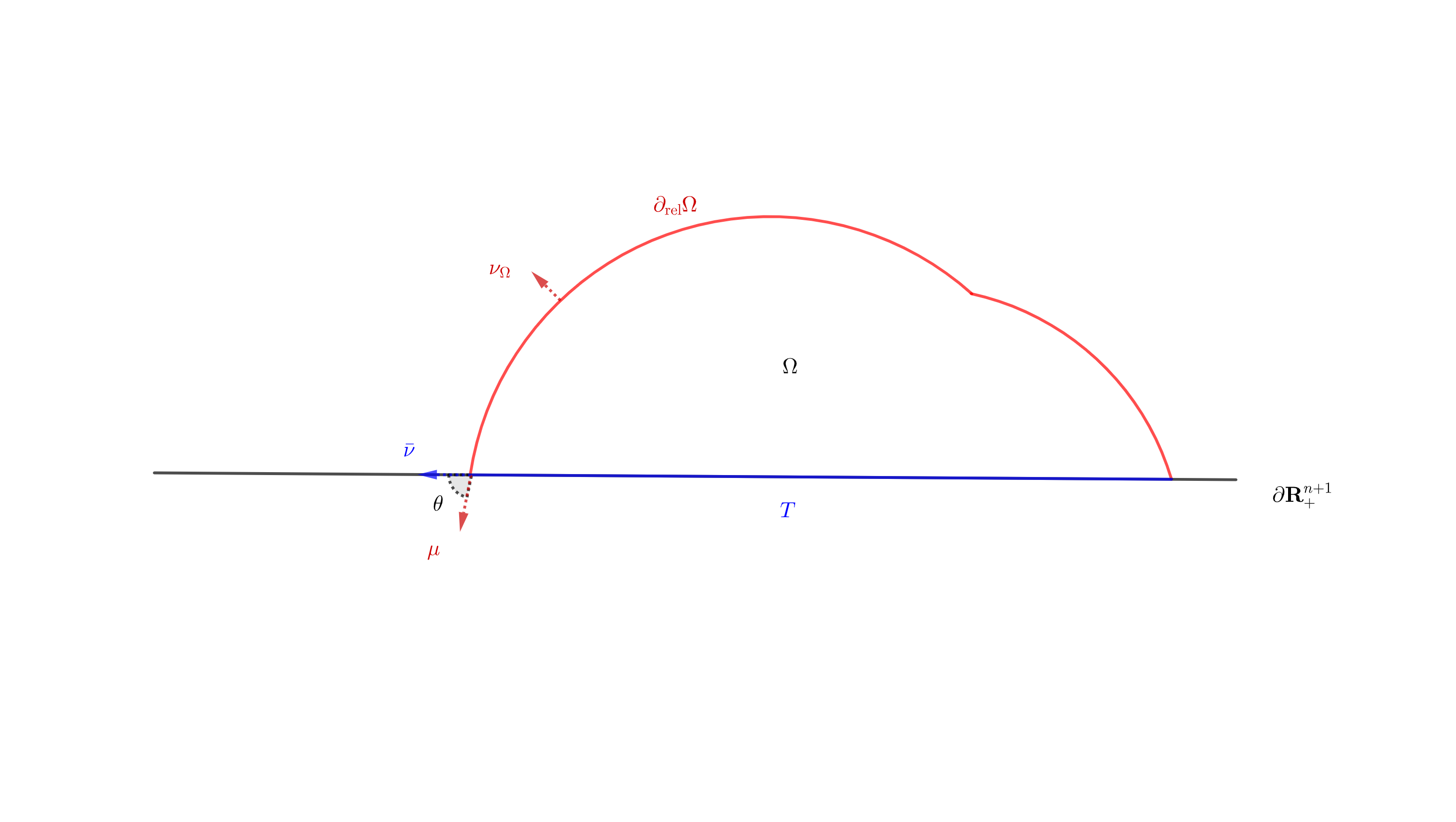
We also denote by ${\rm reg}\Gamma:={\rm reg}\partial_{\rm rel}\Omega\cap\Gamma$ the regular part of $M$ in $\Gamma$ and ${\rm sing}\Gamma=\Gamma\setminus{\rm reg}\Gamma$ the singular part of $M$ in $\Gamma$. Moreover, $\nu_{\Omega}$ denotes the outer unit normal of $\Omega$ along ${\rm reg}\partial_{\rm rel}\Omega$, $H$ denotes the mean curvature of ${\rm reg}\partial_{\rm rel}\Omega$ in $\mathbf{R}^{n+1}$; $\mu,\bar{\nu}$ denote the outer unit conormals of ${\rm reg}\Gamma$ in $\partial_{\rm rel}\Omega$ and ${\rm reg}\Gamma$ in $T$, respectively. We refer to Figure 2 for illustration.

Motivated by Delgadino-Maggi’s work [DM19], a natural question is to characterize the critical points of the $\mathcal{A}$-functional among sets of finite perimeter. This is the main purpose of this paper.

Theorem 1.3.

Given $\theta\in(0,\pi)$ and $c>0$. Let $\Omega\subset\overline{\mathbf{R}^{n+1}_{+}}$ be a bounded, relatively open set of finite perimeter and finite volume, which is stationary for the $\mathcal{A}$-functional. Assume that $\mathcal{H}^{n-1}({\rm sing}\partial_{\rm rel}\Omega)=0$, and $\Gamma$ is a smooth $(n-1)$-manifold in $\partial\mathbf{R}^{n+1}_{+}$. Then $\partial_{\rm rel}\Omega$ must be a finite union of $\theta$-caps and spheres with equal radii.

Remark 1.4.

We make several remarks on the assumptions of our main theorem.

1. For the case $\theta=\pi/2$, the $\mathcal{A}$-stationary set is indeed a critical point of the relative isoperimetric problem (for area functional) in the half-space, and the characterization can be deduced from Delgadino-Maggi’s result. Precisely, provided $\mathcal{H}^{n}({\rm sing}\partial_{\rm rel}\Omega)=0$, $\mathcal{H}^{n-1}({\rm sing}\Gamma)=0$, Allard’s regularity theorem for free boundary rectifiable varifolds [GJ86, Theorem 4.13] implies the young’s law for $\theta=\pi/2$. Hence one may reflect $\partial_{\rm rel}\Omega$ across the hyperplane $\{x_{n+1}=0\}$ and obtain a closed hypersurface $\tilde{\Sigma}$ such that the induced varifold of ${\rm reg}\tilde{\Sigma}$ if of constant generalized mean curvature and $\mathcal{H}^{n}({\rm sing}\tilde{\Sigma})=0$, the assertion then follows from [DM19, Theorem 1].

   In view of the above, we expect that for general $\theta$, the condition $\mathcal{H}^{n-1}({\rm sing}\partial_{\rm rel}\Omega)=0$ in Theorem 1.3 mighted be weakened to $\mathcal{H}^{n}({\rm sing}\partial_{\rm rel}\Omega)=0$, $\mathcal{H}^{n-1}({\rm sing}\Gamma)=0$. Our assumption $\mathcal{H}^{n-1}({\rm sing}\partial_{\rm rel}\Omega)=0$ is technical but crucial for the proof, we delay a detailed illustration to Remark 1.6.

2. The classical Alexandrov’s moving plane method has been extended to the context of integral varifolds by Haslhofer-Hershkovits-White [HHW20], where they made a so-called tameness assumption on integral varifolds [HHW20, Definition 1.6]. The condition that $\Gamma$ is a smooth $(n-1)$-manifold is in fact included in the tameness condition. On the other hand, the assumption that $\Gamma$ is a smooth $(n-1)$-manifold and that $\partial_{\rm rel}\Omega$ is regular enough up to $\Gamma$ for $\mathcal{H}^{n-1}$-a.e. ensures that the Young’s law holds (which provides the contact angle condition). Such $\partial_{\rm rel}\Omega$ will be defined as the singular capillary CMC hypersurface in the half-space in Definition 2.10.

To illustrate the proof, we first make a quick review of Jia-Wang-Xia-Zhang’s argument [Jia+22] in the smooth setting, which can be viewed as the extension of Montiel-Ros’ argument [MR91] to the capillary case. For $\Omega\subset\overline{\mathbf{R}^{n+1}_{+}}$ such that $\partial_{\rm rel}\Omega$ is of CMC and $\partial_{\rm rel}\Omega$ intersects $\partial\mathbf{R}^{n+1}_{+}$ at the angle $\theta$, we define a set

$$Z=\left\{(x,t)\in\partial_{\rm rel}\Omega\times\mathbf{R}:0<t\leq\frac{1}{\max_{i}\kappa_{i}(x)}\right\},$$

and a map which indicates a family of shifted parallel hypersurfaces,

$$\zeta_{\theta}:Z\to\mathbf{R}^{n+1}:\quad\zeta_{\theta}(x,t)=x-t(\nu_{\Omega}-\cos\theta E_{n+1})$$

where $\kappa_{i},i=1\cdots,n$ are the principal curvatures and $\max_{i}\kappa_{i}(x)\geq\frac{H_{\Omega}}{n}>0$. Using the capillary boundary condition, we find that $\zeta_{\theta}$ is surjective onto $\Omega$, namely, $\Omega\subset\zeta_{\theta}(Z)$. By the area formula, we obtain that

$$|\Omega|\leq|\zeta_{\theta}(Z)| \leq\int_{\partial_{\rm rel}\Omega}\int_{0}^{\frac{1}{\max_{i}\kappa_{i}(x)}}(1-\cos\theta\nu_{\Omega}\cdot E_{n+1})\prod_{i=1}^{n}(1-t\kappa_{i}(x)){\rm d}t{\rm d}\mathcal{H}^{n}(x)$$

$$\leq\int_{\partial_{\rm rel}\Omega}\frac{1-\cos\theta\nu_{\Omega}\cdot E_{n+1}}{H_{\Omega}}{\rm d}\mathcal{H}^{n},$$

so that the Heintze-Karcher inequality holds

$$|\Omega|\leq\int_{\partial_{\rm rel}\Omega}\frac{1-\cos\theta\nu_{\Omega}\cdot E_{n+1}}{H_{\Omega}}{\rm d}\mathcal{H}^{n}$$

with equality holds if and only if $\partial_{\rm rel}\Omega$ is a $\theta$-cap. Combining with the Minkowski-type formula

$$\int_{\partial_{\rm rel}\Omega}x\cdot(H_{\Omega}\nu_{\Omega}){\rm d}\mathcal{H}^{n}=\int_{\partial_{\rm rel}\Omega}n(1-\cos\theta\nu_{\Omega}\cdot E_{n+1}){\rm d}\mathcal{H}^{n},$$

we conclude that equality in Heintze-Karcher inequality holds and in turn, $\partial_{\rm rel}\Omega$ is a $\theta$-cap.

Our aim is to generalize the above argument to sets of finite perimeter, in the spirit of Delgadino-Maggi [DM19]. The key ingredient of Delgadino-Maggi’s proof [DM19] is to construct a large subset $\Omega^{\star}$ of good points for a set of finite perimeter $\Omega\subset\mathbf{R}^{n+1}$, with the property that: for the classical parallel hypersurfaces map $\zeta$ considered in [MR91] when restricted to the reduced boundary of $\Omega$, one may show that $|\Omega^{\star}\setminus\zeta(Z)|=0$ and $|\Omega\setminus\Omega^{\star}|=0$, by virtue of which the argument based on the area formula is still applicable. We point out that their construction of $\Omega^{\star}$ is based on a subtle analysis of level-sets of the distance function from boundary, and to adapt their argument to our situation, the first requisite would be to discover a suitable capillary counterpart of the distance function considered in [DM19]. This is done in light of the following observation.

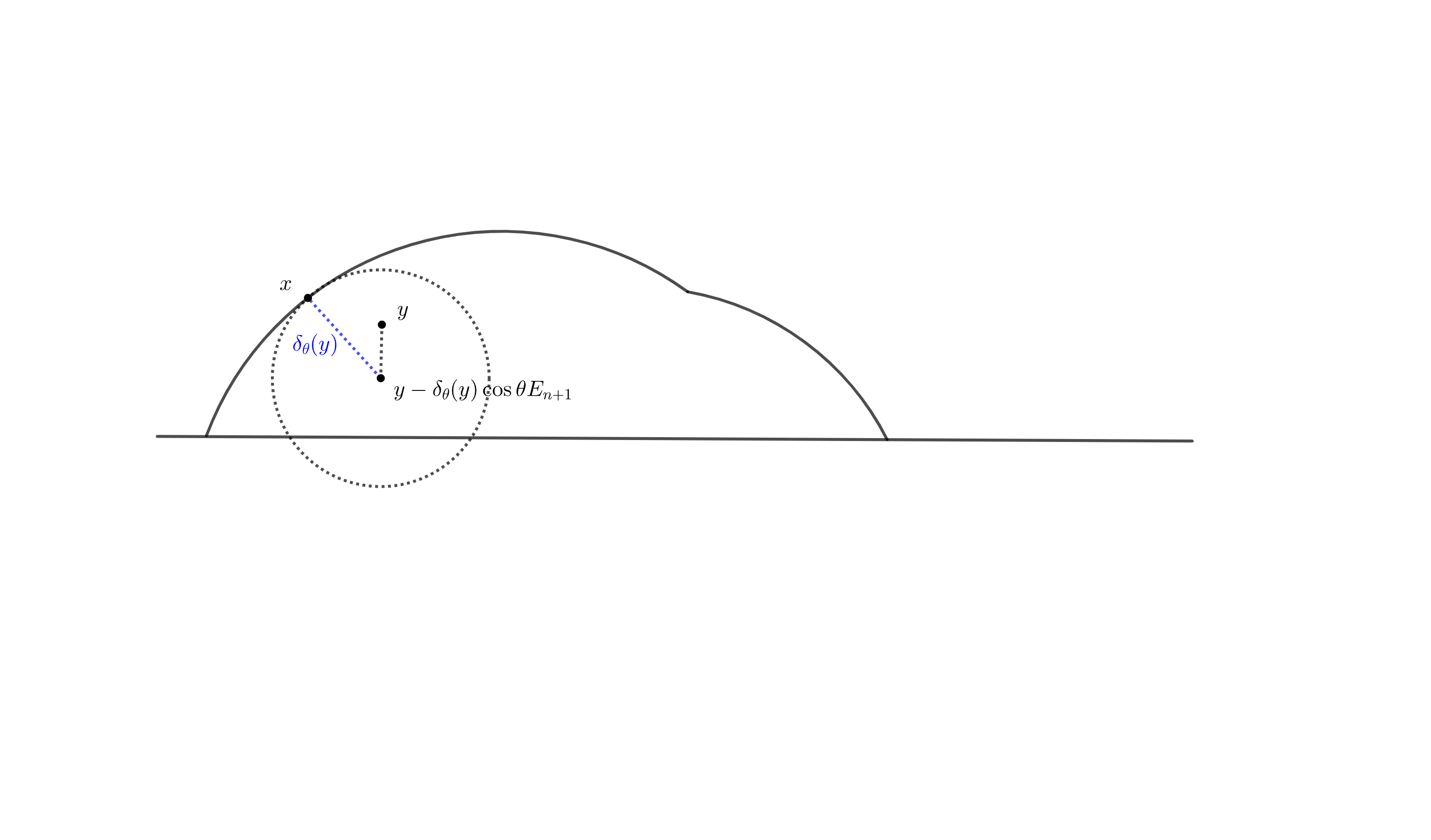
In the proof of Jia-Wang-Xia-Zhang [Jia+22], to show the surjectivity of $\zeta_{\theta}$, we have to show that for any $y\in\Omega$, there is always some $x\in\Sigma$ such that $y$ can be flowed from $x$ through $\zeta_{\theta}$. To this end, we consider the following foliation $\{\partial B_{r}(y-r\cos\theta E_{n+1})\}_{r\geq 0}$, and we are concerned with the first touching point of the foliation with $\Sigma$, when the radius increases from $0$. The first touching point in this case somehow serves as a shifted ‘unique point projection’ from $y$ to $\Sigma$, which motivates the following definition of shifted distance function. Given a bounded, relatively open set of finite perimeter $\Omega\subset\overline{\mathbf{R}^{n+1}_{+}}$ and $\theta\in(0,\pi)$, let $\delta:\mathbf{R}^{n+1}\to\mathbf{R}$ be the distance function with respect to $\partial_{\rm rel}\Omega$, defined as

$$\delta(y)=\sup_{r\geq 0}\{r:B_{r}(y)\cap\partial_{\rm rel}\Omega=\varnothing\}.$$ (1.2)

and $\delta_{\theta}:\mathbf{R}^{n+1}\to\mathbf{R}$ be the shifted distance function with respect to $\partial_{\rm rel}\Omega$ and $\theta$, defined as

$$\delta_{\theta}(y)=\sup_{r\geq 0}\{r:B_{r}(y-r\cos\theta E_{n+1})\cap\partial_{\rm rel}\Omega=\varnothing\}.$$ (1.3)

One sees from definition that

$$\delta_{\theta}(y)=\delta(y-\delta_{\theta}(y)\cos\theta E_{n+1})$$ (1.4)

and for any $0<r<\delta_{\theta}(y)$, there holds

$$\delta(y-r\cos\theta E_{n+1})>r.$$ (1.5)

See Figure 1.

Figure 1. shifted distance function

For $s>0$, we define the super level-set and level-set of $\delta_{\theta}$ in $\overline{\Omega}$ by

$$\Omega_{s}:=\{y\in\overline{\Omega}:\delta_{\theta}(y)>s\},\quad\partial_{\rm rel}\Omega_{s}:=\{y\in\overline{\Omega}:\delta_{\theta}(y)=s\}.$$ (1.6)

$\delta_{\theta}$ indeed plays the same role as the distance function considered in [DM19], and we may adapt Delgadino-Maggi’s approach to define the large subset $\Omega^{\star}_{\theta}$ of good points in our setting as follows.

Definition 1.5 ($\Gamma_{s;\theta}^{t}$ and $\Gamma_{s;\theta}^{+}$).

Let $\Omega$ be a bounded, relatively open set of finite perimeter in $\overline{\mathbf{R}^{n+1}_{+}}$ and $\theta\in(0,\pi)$. For every $0<s<t<\infty$, we define $\Gamma_{s;\theta}^{t}$ to be the set of $y\in\partial_{\rm rel}\Omega_{s}$ such that there exists a geodesic $\gamma_{y}:[0,t]\to\mathbf{R}^{n+1}$ with $\gamma_{y}(s)=y$ and $\delta_{\theta}(\gamma_{y}(r))=r$ for every $r\in[0,t]$.

Moreover, for every $0<s<\infty$, define

$$\Gamma_{s;\theta}^{+}=\bigcup_{t>0}\Gamma_{s;\theta}^{t},\quad\Omega^{\star}_{\theta}=\bigcup_{s>0}\Gamma_{s;\theta}^{+}.$$

In the first step, we shall prove that $\Gamma_{s;\theta}^{t}$ is $C^{1,1}$-rectifiable (Theorem 3.1). Our strategy for proving the $C^{1,1}$-rectifiability theorem in terms of the shifted distance function follows largely from [DM19, Theorem 1, step 1]. With the $C^{1,1}$-rectifiability theorem, we are able to prove that $|\Omega\setminus\Omega^{\star}_{\theta}|=0$. Next, we prove $|\Omega^{\star}_{\theta}\setminus\zeta_{\theta}(Z)|=0$, following [DM19, Theorem 1, step 4]. In contrast to the closed hypersurface case in [DM19, Theorem 1, step 4], here we have to carefully deal with the boundary of the singular capillary CMC hypersurface $\partial_{\rm rel}\Omega$ (see Definition 2.10 for the definition). Indeed, a crucial issue to be clarified is the counting measure of $g_{s;\theta}^{-1}(x)$ for $x\in{\rm reg}\partial_{\rm rel}\Omega$ (see the proof of Theorem 1.3 for the definition of $g_{s;\theta}^{-1}$), and when $x$ lies in the interior of $\partial_{\rm rel}\Omega$, i.e., $x\in\partial_{\rm rel}\Omega\setminus\Gamma$, we could use the same argument in [DM19], by studying the blow-up feature of $\partial_{\rm rel}\Omega$ at $x$, and the maximum principle for stationary rectifiable cones, to conclude that the counting measure is at most $2$. Likewise, we have to study the boundary behaviors of $\partial_{\rm rel}\Omega$ and $T$ along $\Gamma$, and consider the blow-up process at every $x\in\Gamma$. To this end, we first introduce a new definition of $\theta$-stationary triple in Definition 2.13 (which is satisfied by the blow-up limit of the singular capillary CMC hypersurface under our regularity assumption in Theorem 1.3), and then we exploit new boundary strong maximum principles Lemma 2.16, Lemma 2.17 to study the blow-up process.

Once the properties $|\Omega\setminus\Omega^{\star}_{\theta}|=0$ and $|\Omega^{\star}_{\theta}\setminus\zeta_{\theta}(Z)|=0$ are established, we can proceed Jia-Wang-Xia-Zhang’s argument [Jia+22] in the framework of sets of finite perimeter.

In the end, we make further comments on the technical assumption $\mathcal{H}^{n-1}({\rm sing}\partial_{\rm rel}\Omega)=0$ in Theorem 1.3.

Remark 1.6.

As already discussed, in Theorem 1.3 $\mathcal{H}^{n-1}({\rm sing}\partial_{\rm rel}\Omega)=0$ is a technical but crucial assumption. Here we make some illustrations.

1. To study the boundary behavior of $\partial_{\rm rel}\Omega$ and $T$ along $\Gamma$, we need to consider the $\theta$-stationary triple, which is well-defined thanks to Lemma 2.8. The proof of Lemma 2.8 is built on the smooth cut-off functions near singularities of $\partial_{\rm rel}\Omega$, whose existence relies largely on the assumption that $\mathcal{H}^{n-1}({\rm sing}\partial_{\rm rel}\Omega)=0$.

2. As we have mentioned in Remark 1.4(1), Young’s law can be deduced from $\mathcal{H}^{n}({\rm sing}\partial_{\rm rel}\Omega)=\mathcal{H}^{n-1}({\rm sing}\Gamma)=0$ and the $\mathcal{A}$-stationarity of $\Omega$ thanks to the Allard’s regularity theorem for free boundary rectifiable varifolds [GJ86, Theorem 4.13]. However, it is still an open question whether an Allard-type regularity theorem holds for capillary submanifolds with general contact angles. Despite the lack of the Allard-type regularity result, we could still obtain Young’s law for $\mathcal{A}$-stationary set in Proposition 2.9, provided that $\mathcal{H}^{n-1}({\rm sing}\partial_{\rm rel}\Omega)=0$.

Organization of the paper. In Section 2 we collect some background material from geometric measure theory and prove the boundary maximum principles that are useful for the blow-up analysis in the proof of the Alexandrov-type theorems. In Section 3 we study the fine properties of $\Gamma_{s;\theta}^{t}$ and then we prove the rectifiability result Theorem 3.1. In Section 4, we prove our main result Theorem 1.3.

Acknowledgements. We are indebted to Professor Guofang Wang for stimulating discussions on this topic and his constant support.

2. Preliminaries

2.1. Notations

When considering the topology of $\mathbf{R}^{n+1}$, we denote by $\overline{\Omega}$ the topological closure of a set $\Omega$, by ${\rm int}(\Omega)$ the topological interior of $\Omega$, and by $\partial\Omega$ the topological boundary of $\Omega$. In terms of the subspace topology (relative topology), we use the following notations: let $X$ be a topological space and $S$ be a subspace of $X$, we use ${\rm cl}_{X}S,{\rm int}_{X}S,\partial_{X}S$ to denote the closure, the interior, and the boundary, respectively, of $S$ in the topological space $X$. In particular, for a bounded, relatively open set of finite perimeter $\Omega\subset\overline{\mathbf{R}^{n+1}_{+}}$. We denote by $\partial_{\rm rel}\Omega:=\partial_{\overline{\mathbf{R}^{n+1}_{+}}}\Omega=\overline{\partial\Omega\cap\mathbf{R}^{n+1}_{+}}$ the relative boundary of $\Omega$ in the upper half-space $\overline{\mathbf{R}^{n+1}_{+}}$, let $T:={\rm cl}_{\partial\mathbf{R}^{n+1}_{+}}\left(\partial\Omega\setminus\partial_{\rm rel}\Omega\right)$, and denote by $\Gamma:=\partial_{\rm rel}\Omega\cap\partial\mathbf{R}^{n+1}_{+}$, see Figure 2 for illustration.

Figure 2. Notations

• $\boldsymbol{\mu}_{r}$ is the homothety map $y\mapsto ry$;

• $\boldsymbol{\tau}_{x}$ is the translation map $y\mapsto y-x$;

• $\boldsymbol{\eta}_{x,r}$ is the composition $\boldsymbol{\mu}_{r^{-1}}\circ\boldsymbol{\tau}_{x}$, i.e., $y\mapsto\frac{y-x}{r}$;

• $\mathcal{H}^{k}$ is the $k$-dimensional Hausdorff measure on $\mathbf{R}^{n+1}$;

• $\mathcal{L}^{n+1}$ is the Lebesgue outer measure on $\mathbf{R}^{n+1}$;

• $B_{r}(x)$ is the open ball in $\mathbf{R}^{n+1}$, centered at $x$ with radius $r$;

• $\omega_{n}$ is the volume of the $n$-dimensional unit ball in $\mathbf{R}^{n+1}$;

• ${\rm spt}$ is the support of a measure, see [Mag12, Section 2.4].

• In this paper, we work with the following spaces of vector fields:

  $$\mathfrak{X}_{c}(\mathbf{R}^{n+1}):=\{\text{the space of all $C^{1}$-vector fields on }\mathbf{R}^{n+1}\text{ with compact support}\},$$

  $$\mathfrak{X}(\overline{\mathbf{R}^{n+1}_{+}}):=\left\{X\in\mathfrak{X}_{c}(\mathbf{R}^{n+1}):X(p)\in T_{p}\overline{\mathbf{R}^{n+1}_{+}}\text{ for all }p\in\overline{\mathbf{R}^{n+1}_{+}}\right\},$$

  $$\mathfrak{X}_{c}(\overline{\mathbf{R}^{n+1}_{+}}):=\left\{X\in\mathfrak{X}(\overline{\mathbf{R}_{+}^{n+1}}):X\text{ has relatively compact support in the open half-space }\mathbf{R}^{n+1}_{+}\right\},$$

  $$\mathfrak{X}_{t}(\overline{\mathbf{R}^{n+1}_{+}}):=\left\{X\in\mathfrak{X}(\overline{\mathbf{R}^{n+1}_{+}}):X(p)\in T_{p}(\partial\mathbf{R}^{n+1}_{+})\text{ for all }p\in\partial\mathbf{R}^{n+1}_{+}\right\}.$$

  Notice that at any $x\in\partial\mathbf{R}^{n+1}_{+}$, $T_{x}\mathbf{R}^{n+1}_{+}$ is exactly the $(n+1)$-dimensional half-space in $\mathbf{R}^{n+1}$ with boundary $T_{x}\partial\mathbf{R}^{n+1}_{+}$.

2.2. Rectifiable sets

A Borel set $M\subset\mathbf{R}^{n+1}$ is a locally $\mathcal{H}^{n}$-rectifiable set if $M$ can be covered, up to a $\mathcal{H}^{n}$-negligible set, by countably many Lipschitz images of $\mathbf{R}^{n}$ into $\mathbf{R}^{n+1}$, and if $\mathcal{H}^{n}\llcorner M$ is locally finite on $\mathbf{R}^{n+1}$. $M$ is called $\mathcal{H}^{n}$-rectifiable if, in addition, $\mathcal{H}^{n}(M)<\infty$; $M$ is called normalized, if $M={\rm spt}(\mathcal{H}^{n}\llcorner M)$, i.e.,

$$x\in M\quad\text{if and only if }\mathcal{H}^{n}(B_{\rho}(x)\cap M)>0\quad\text{for all }\rho>0.$$

Proposition 2.1 (area formula for $k$-rectifiable sets, [Mag12, Theorem 11.6]).

For $1\leq k\leq m$, if $A\subset\mathbf{R}^{n}$ is a locally $\mathcal{H}^{k}$-rectifiable set and $f:\mathbf{R}^{n}\rightarrow\mathbf{R}^{m}$ is a Lipschitz map, then

$$\int_{\mathbf{R}^{m}}\mathcal{H}^{0}\left(A\cap\left\{f=y\right\}\right){\rm d}\mathcal{H}^{k}(y)=\int_{A}{\rm J}^{A}f(x){\rm d}\mathcal{H}^{k}(x),$$ (2.1)

where $\left\{f:=y\right\}=\left\{x\in\mathbf{R}^{n}:f(x)=y\right\}$, ${\rm J}^{A}f(x)$ is the Jacobian of $f$ with respect to $A$ at $x$ (see for example [Mag12, (11.1)]), which exsits for $\mathcal{H}^{k}$-a.e. $x\in A$.

Lemma 2.2 (tangential property of Lipschitz function along rectifiable sets, [DM19, Section 2.1(iv)]).

Let $M\subset\mathbf{R}^{n+1}$ be a locally $\mathcal{H}^{n}$-rectifiable set and $f:M\rightarrow\mathbf{R}^{n+1}$ is a Lipschitz map defined on $M$, then for any Lipschitz functions $F,G:\mathbf{R}^{n+1}\rightarrow\mathbf{R}^{n+1}$ such that $F=G=f$ on $M$, we have

$$\nabla^{M}F=\nabla^{M}G\quad\mathcal{H}^{n}\text{-a.e. on }M.$$ (2.2)

In particular, if $g:\mathbf{R}^{n}\rightarrow\mathbf{R}^{n+1}$ is a Lipschitz map and $E\subset\mathbf{R}^{n}$ is a Borel set, then $T_{x}M=(\nabla g)_{g^{-1}(x)}[\mathbf{R}^{n}]$ for $\mathcal{H}^{n}$-a.e. $x\in M\cap g(E)$, with

$$(\nabla^{M}F)_{x}[\tau]=\nabla(F\circ g)_{g^{-1}(x)}[(\nabla g)_{x}^{-1}[\tau]]\quad\forall\tau\in T_{x}M.$$ (2.3)

Here $\nabla^{M}F(x)$ denotes the tangential differential of $F$ with respect to $M$ at $x$, which exsits for $\mathcal{H}^{n}$-a.e. $x\in M$ by virtue of the Rademacher-type theorem [Mag12, Theroem 11.4].

2.3. Rectifiable varifolds

We now quickly recall some basic notions of rectifiable varifolds in $\mathbf{R}^{n+1}$, and we refer to the standard references [All72, Sim83] for details.

Let $M$ be a locally $\mathcal{H}^{k}$-rectifiable set and consider a Borel measurable function $\psi\in L^{1}_{\rm loc}(\mathcal{H}^{k}\llcorner M;\mathbf{R}^{+})$. The rectifiable varifold $V={\rm var}(M,\psi)$ defined by $M$ and $\psi$ is the Radon measure on $\mathbf{R}^{n+1}\times G(n+1,k)$, defined as

$$\int_{\mathbf{R}^{n+1}\times G(n+1,k)}\Phi{\rm d}{\rm var}(M,\psi)=\int_{M}\Phi(x,T_{x}M)\psi(x){\rm d}\mathcal{H}^{k}(x),$$

for every bounded, compactly supported Borel function $\Phi$ on $\mathbf{R}^{n+1}\times G(n+1,k)$. In particular, for any $X\in\mathfrak{X}_{c}(\mathbf{R}^{n+1})$, the well-known first variatioanl formula reads

$$\delta{\rm var}(M,\psi)[X]=\int_{M}{\rm div}_{M}X(x)\psi(x){\rm d}\mathcal{H}^{k}(x).$$

The weight measure of $V={\rm var}(M,\psi)$ is denoted by $||V||=\psi\mathcal{H}^{k}\llcorner M$. As in [Sim83, Definition 42.3], we denote ${\rm VarTan(V,x)}$ to be the set of varifold tangents of $V$ at some $x\in{\rm spt}||V||.$ By the compactness of Radon measures [Sim83, Theorem 4.4], ${\rm VarTan}(V,x)$ is compact and non-empty provided that the upper density $\Theta^{\ast k}(||V||,x)$ is finite.

Definition 2.3 (Stationary varifolds).

A rectifiable varifold ${\rm var}(M,\psi)$ is said to be stationary in $\mathbf{R}^{n+1}$ if $\delta{\rm var}(M,\psi)[X]=0$ for any $X\in\mathfrak{X}_{c}(\mathbf{R}^{n+1})$, and is said to be stationary in $\overline{\mathbf{R}^{n+1}_{+}}$ with free boundary if $\delta{\rm var}(M,\psi)[X]=0$ for any $X\in\mathfrak{X}_{t}(\overline{\mathbf{R}^{n+1}_{+}})$.

The following useful reflection trick will be needed in our proof, see [All75, (3.2)], [GJ86, Remark 4.11(iii)] and [LZ21, Lemma 2.2].

Lemma 2.4 (Reflection Principle).

Let $E_{n+1}:=(0,\ldots,0,1)\in\overline{\mathbf{R}^{n+1}_{+}}$. Let $\theta_{n+1}:\mathbf{R}^{n+1}\rightarrow\mathbf{R}^{n+1}$ denote the reflection map about the unit vector $E_{n+1}$, i.e., $\theta_{n+1}(u)=u-2(u\cdot E_{n+1})E_{n+1}$. For any rectifiable varifold $V:={\rm var}(M,\psi)$, define the doubled varifold

$$\bar{V}:=V+(\theta_{n+1})_{\#}V.$$ (2.4)

If $V$ is stationary in $\overline{\mathbf{R}^{n+1}_{+}}$ with free boundary, then $\bar{V}$ is stationary in $\mathbf{R}^{n+1}$.

2.4. Sets of finite perimeter

For basic knowledge regarding sets of finite perimeter, we refer to the monograph [Mag12] (in particular, Chapter 15) for a detailed account.

Given a Lebesgue measurable set $\Omega\subset\mathbf{R}^{n+1}$, we say that $\Omega$ is a set of finite perimeter in $\mathbf{R}^{n+1}$ if

$$\sup\left\{\int_{\mathbf{R}^{n+1}}{\rm div}X{\rm d}\mathcal{L}^{n+1}:X\in C^{1}_{c}(\mathbf{R}^{n+1};\mathbf{R}^{n+1}),|X|\leq 1\right\}<\infty.$$

An equivalent characterization of sets of finite perimeter (see [Mag12, Proposition 12.1]) is that: there exists a $\mathbf{R}^{n+1}$-valued Radon measure $\mu_{\Omega}$ on $\mathbf{R}^{n+1}$ such that for any $X\in C_{c}^{1}(\mathbf{R}^{n+1};\mathbf{R}^{n+1})$,

$$\int_{\Omega}{\rm div}X{\rm d}\mathcal{L}^{n+1}=\int_{\mathbf{R}^{n+1}}X\cdot{\rm d}\mu_{\Omega}.$$ (2.5)

$\mu_{\Omega}$ is called the Gauss-Green measure of $\Omega$. The relative perimeter of $\Omega$ in $E\subset\mathbf{R}^{n+1}$, and the perimeter of $\Omega$, are defined as

$$P(\Omega;E)=|\mu_{\Omega}|(E),\quad P(\Omega)=|\mu_{\Omega}|(\mathbf{R}^{n+1}).$$

Regarding the topological boundary of a set of finite perimeter $E$, one has (see [Mag12, Proposition 12.19])

$${\rm spt}\mu_{\Omega}=\{x\in\mathbf{R}^{n+1}:0<|\Omega\cap B_{r}(x)|<\omega_{n+1}r^{n+1},\quad\forall r>0\}\subset\partial\Omega.$$

The reduced boundary $\partial^{\ast}\Omega$ is the set of those $x\in{\rm spt}\mu_{\Omega}$ such that the limit

$$\lim_{r\rightarrow 0^{+}}\frac{\mu_{\Omega}(B_{r}(x))}{|\mu_{\Omega}|(B_{r}(x))}\text{ exists and belongs to }\mathbf{S}^{n}.$$

The Borel vector field $\nu_{\Omega}:\partial^{\ast}\Omega\rightarrow\mathbf{S}^{n}$ is called the measure-theoretic outer unit normal to $\Omega$, and there holds

$$\overline{\partial^{\ast}\Omega}={\rm spt}\mu_{\Omega}.$$

Moreover, when $\Omega$ is a bounded, relatively open set of finite perimeter in $\overline{\mathbf{R}^{n+1}_{+}}$, the reduced boundary is locally $\mathcal{H}^{n}$-rectifiable and the sets $\partial_{\rm rel}\Omega,T$ are normalized. By [DM15, (2.1)],

$$\mu_{\Omega}=\nu_{\Omega}\mathcal{H}^{n}\llcorner(\partial^{\ast}\Omega\cap\mathbf{R}^{n+1}_{+})-E_{n+1}\mathcal{H}^{n}\llcorner(\partial^{\ast}\Omega\cap\partial\mathbf{R}^{n+1}_{+}),$$

and thus (2.5) reads

$$\int_{\Omega}{\rm div}X{\rm d}\mathcal{L}^{n+1}=\int_{\partial^{\ast}\Omega\cap\mathbf{R}^{n+1}_{+}}X\cdot\nu_{\Omega}{\rm d}\mathcal{H}^{n}-\int_{\partial^{\ast}\Omega\cap\partial\mathbf{R}^{n+1}_{+}}X\cdot E_{n+1}{\rm d}\mathcal{H}^{n}.$$

Under the regularity assumption $\mathcal{H}^{n}({\rm sing}\partial_{\rm rel}\Omega)=0$, the above equality then takes the form

$$\int_{\Omega}{\rm div}X{\rm d}\mathcal{L}^{n+1}=\int_{\partial_{\rm rel}\Omega}X\cdot\nu_{\Omega}{\rm d}\mathcal{H}^{n}-\int_{T}X\cdot E_{n+1}{\rm d}\mathcal{H}^{n}.$$ (2.6)

To every set of finite perimeter in $\overline{\mathbf{R}^{n+1}_{+}}$, we can always associate in a natural way the integer rectifiable varifolds ${\rm var}(\partial^{\ast}\Omega\cap\mathbf{R}^{n+1}_{+},1)$ and ${\rm var}(\partial^{\ast}\Omega\cap\partial\mathbf{R}^{n+1}_{+},1)$. For simplicity we denote them respectively by ${\rm var}(\partial^{\ast}\Omega\cap\mathbf{R}^{n+1}_{+})$ and ${\rm var}(\partial^{\ast}\Omega\cap\partial\mathbf{R}^{n+1}_{+})$.

2.5. Critical points of the $\mathcal{A}$-functional

Recall that the $\mathcal{A}$-functional is defined in Definition 1.1, which follows from [LZZ21, Definition 1.1]. In fact, given $\theta\in(0,\pi)$, a constant $c>0$, and a set of finite perimeter $\Omega$ as in Definition 1.1, the first variation for $\mathcal{A}$ along $X\in\mathfrak{X}(\overline{\mathbf{R}^{n+1}_{+}})$ is (see [LZZ21, (1.7)])

$$\delta\mathcal{A}\mid_{\Omega}(X)=\int_{\partial^{\ast}\Omega\llcorner\mathbf{R}^{n+1}_{+}}{\rm div}_{\partial\Omega}X{\rm d}\mathcal{H}^{n}+\cos(\pi-\theta)\int_{\partial^{\ast}\Omega\llcorner\partial\mathbf{R}^{n+1}_{+}}{\rm div}_{\partial\Omega}X{\rm d}\mathcal{H}^{n}-c\int_{\partial^{\ast}\Omega}X\cdot\nu_{\Omega}{\rm d}\mathcal{H}^{n},$$ (2.7)

which implies the following facts: if $\Omega$ is stationary for $\mathcal{A}$ as in Definition 1.1, then

1. when $\theta\in(0,\pi)$, $\Omega$ is stationary for the free energy functional

   $$\mathcal{E}(\Omega)=P(\Omega;\mathbf{R}^{n+1}_{+})-\cos\theta P(\Omega;\partial\mathbf{R}^{n+1}_{+}).$$

   under volume constraint, see e.g., [XZ21, Definition 4.2], and the reason is that the first variation of $|\Omega|$ along $X$ is indeed given by $\int_{\partial^{\ast}\Omega}X\cdot\nu_{\Omega}{\rm d}\mathcal{H}^{n}$, see [Mag12, (17.31)].

2. when $\theta\in[\pi/2,\pi)$, the naturally induced varifold ${\rm var}(\partial^{\ast}\Omega\cap\mathbf{R}^{n+1}_{+})$ has a fixed contact angle $\theta$ with $\partial\mathbf{R}^{n+1}_{+}$ at $\partial^{\ast}\Omega\cap\partial\mathbf{R}^{n+1}_{+}$ in the sense of [KT17, Definition 3.1] with generalized mean curvature $H=c$, since for any $X\in\mathfrak{X}_{t}(\overline{\mathbf{R}^{n+1}_{+}})$, (2.7) reads as

   $$\int_{\partial^{\ast}\Omega\llcorner\mathbf{R}^{n+1}_{+}}{\rm div}_{\partial\Omega}X{\rm d}\mathcal{H}^{n}+\cos(\pi-\theta)\int_{\partial^{\ast}\Omega\llcorner\partial\mathbf{R}^{n+1}_{+}}{\rm div}_{\partial\mathbf{R}^{n+1}_{+}}X{\rm d}\mathcal{H}^{n}=\int_{\partial^{\ast}\Omega\llcorner\mathbf{R}^{n+1}_{+}}X\cdot(c\nu_{\Omega}){\rm d}\mathcal{H}^{n}.$$ (2.8)

   Moreover, the naturally induced pair of varifolds $\left({\rm var}(\partial^{\ast}\Omega\cap\mathbf{R}^{n+1}_{+}),{\rm var}(\partial^{\ast}\Omega\cap\partial\mathbf{R}^{n+1}_{+})\right)$ satisfies the contact angle condition $\theta$ in the sense of [DD21, Definition 3.1].

   For the case $\theta\in(0,\pi/2)$, we have the following observation.

   Remark 2.5.

   When the capillary angle $\theta\in(0,\pi/2)$, since we consider only the sets of finite perimeter that are bounded, we may assume that there is a large enough smooth open set $\mathbf{B}_{+}$ such that $\Omega\subset\mathbf{B}_{+}\subset\overline{\mathbf{R}^{n+1}_{+}}$. Once the set $\mathbf{B}_{+}$ is fixed, we know that $P(\mathbf{B}_{+};\partial\mathbf{R}^{n+1}_{+})$ is a fixed number and it is clear that

   $$P(\Omega;\partial\mathbf{R}^{n+1}_{+})=P(\mathbf{B}_{+};\partial\mathbf{R}^{n+1}_{+})-P(\mathbf{B}_{+}\setminus\Omega;\partial\mathbf{R}^{n+1}_{+}),$$

   which implies the following fact: if $\Omega$ is $\mathcal{A}$-stationary (as in Definition 1.1), then it is stationary for the modified functional

   $$\tilde{\mathcal{A}}(\Omega):=P(\Omega;\mathbf{R}^{n+1}_{+})+\cos\theta P(\mathbf{B}_{+}\setminus\Omega;\partial\mathbf{R}^{n+1}_{+})-c|\Omega|,$$ (2.9)

   in the sense that for any $C^{1}$-diffeomorphism $f:\overline{\mathbf{R}^{n+1}_{+}}\rightarrow\overline{\mathbf{R}^{n+1}_{+}}$ with ${\rm spt}f\subset\subset\overline{\mathbf{B}_{+}}$, such that $f:\partial\mathbf{R}^{n+1}_{+}\rightarrow\partial\mathbf{R}^{n+1}_{+}$ is a diffeomorphism of $\partial\mathbf{R}^{n+1}_{+}$, there holds

   $$\frac{{\rm d}}{{\rm d}t}\mid_{t=0}\tilde{\mathcal{A}}(\psi_{t}(\Omega))=0,$$

   where $\{\psi_{t}\}_{|t|<T}$ is a one parameter family of diffeomorphisms induced by $f$.

An important feature we shall use for the $\mathcal{A}$-stationary sets is that they satisfy the following Euclidean volume growth condition:

Proposition 2.6.

Given $\theta\in(0,\pi)$ and $c>0$. Let $\Omega\subset\overline{\mathbf{R}^{n+1}_{+}}$ be a non-empty, bounded, relatively open set with finite perimeter in $\overline{\mathbf{R}^{n+1}_{+}}$ that is stationary for the $\mathcal{A}$-functional, then $\partial_{\rm rel}\Omega$ has Euclidean volume growth, that is, there exists some universal constants (depends only on $\Omega$ and $n$) $R_{1}>0$ and $C_{1}>0$ such that for any $x\in\partial_{\rm rel}\Omega$ and for any $0<r<R_{1}$, there holds

$$\mathcal{H}^{n}(\partial_{\rm rel}\Omega\cap B_{r}(x))\leq C_{1}r^{n}.$$ (2.10)

Proof.

Case 1. $\theta\in[\pi/2,\pi)$.

Our starting point is that as illustrated below (2.7), ${\rm var}(\partial^{\ast}\Omega\llcorner\mathbf{R}^{n+1}_{+})$ has a fixed contact angle $\theta$ with $\partial\mathbf{R}^{n+1}_{+}$ at $\partial^{\ast}\Omega\llcorner\partial\mathbf{R}^{n+1}_{+}$ in the sense of [KT17, Definition 3.1] with bounded generalized mean curvature, therefore the monotonicity formula [KT17, Theorem 3.2] is applicable here. Moreover, since $\partial\mathbf{R}^{n+1}_{+}$ is planar, we know that the maximal distance ($s_{0}$) used to define the tubular neighborhood ($N_{s_{0}}$) in [KT17] can be taken as large as possible in our case. By taking $s_{0}=6\cdot{\rm diam}(\Omega):=6\cdot\max_{x,y\in\overline{\Omega}}|x-y|$ and fix $p=n+1$ in [KT17, (3.9)], we find: for any $x\in\partial_{\rm rel}\Omega$ and for any $0<r<{\rm diam}(\Omega)$,

$$\frac{\mathcal{H}^{n}(\partial_{\rm rel}\Omega\cap B_{r}(x))}{r^{n}}\leq\omega_{n}\left\{\left(\frac{2\mathcal{H}^{n}(\partial^{\ast}\Omega)}{\omega_{n}({\rm diam}(\Omega))^{n}}\right)^{\frac{1}{n+1}}+\gamma\cdot({\rm diam}(\Omega))^{\frac{1}{n+1}}\right\}^{n+1}:=C,$$

where $\gamma:=\left(\frac{1}{\omega_{n}}\int_{\partial^{\ast}\Omega\cap\mathbf{R}^{n+1}_{+}}2|H(x)|^{n+1}{\rm d}\mathcal{H}^{n}(x)\right)^{\frac{1}{n+1}}$ is bounded since $\Omega$ is of finite perimeter and $|H|=c$ (which follows from the $\mathcal{A}$-stationarity of $\Omega$), and hence

$$\mathcal{H}^{n}(\partial_{\rm rel}\Omega\cap B_{r}(x))\leq Cr^{n}$$

for every $x\in\partial_{\rm rel}\Omega$, $r<{\rm diam}(\Omega)$. This shows that $\partial_{\rm rel}\Omega$ has Euclidean volume growth.

Case 2. $\theta\in(0,\pi/2)$.

Recall Remark 2.5, ${\rm var}(\partial^{\ast}\Omega\cap\mathbf{R}^{n+1}_{+})$ has a fixed contact angle $\tilde{\theta}:=\pi-\theta\in(\pi/2,\pi)$ with $\partial\mathbf{R}^{n+1}_{+}$ at $\partial^{\ast}(\mathbf{B}_{+}\setminus\Omega)\cap\partial\mathbf{R}^{n+1}_{+}$ in the sense of [KT17, Definition 3.1] with generalized mean curvature $H=c$, a simple modification of Case 1 then shows that: when $\theta\in(0,\pi/2)$, $\partial_{\rm rel}\Omega$ satisfies the Euclidean volume growth condition as well. This completes the proof. ∎

Remark 2.7.

Our main theorem is stated under the regularity assumption that $\mathcal{H}^{n-1}({\rm sing}\partial_{\rm rel}\Omega)=0$. In light of the Hausdorff dimension of the singular set, in all follows, we do not make a distinction between the integrals $\int_{\partial_{\rm rel}\Omega}\cdot{\rm d}\mathcal{H}^{n}$, $\int_{\partial^{\ast}\Omega\cap\mathbf{R}^{n+1}_{+}}\cdot{\rm d}\mathcal{H}^{n}$ and $\int_{{\rm reg}\partial_{\rm rel}\Omega}\cdot{\rm d}\mathcal{H}^{n}$; $\int_{\Gamma}\cdot{\rm d}\mathcal{H}^{n-1}$ and $\int_{{\rm reg}\Gamma}\cdot{\rm d}\mathcal{H}^{n-1}$.

Under the regularity assumption, we have the following useful tangential divergence theorem for the $\mathcal{A}$-stationary set, whose proof is postponed to Appendix A.

Lemma 2.8.

Given $\theta\in(0,\pi)$ and $c>0$, let $\Omega$ be a non-empty, bounded, relatively open set with finite perimeter in $\overline{\mathbf{R}^{n+1}_{+}}$ such that $\mathcal{H}^{n-1}({\rm sing}\partial_{\rm rel}\Omega)=0$. If $\Omega$ is stationary for the $\mathcal{A}$-functional, then for any $X\in\mathfrak{X}(\overline{\mathbf{R}^{n+1}_{+}})$, there holds

$$\int_{\partial_{\rm rel}\Omega}{\rm div}_{\partial\Omega}X{\rm d}\mathcal{H}^{n}=\int_{\Gamma}X\cdot\mu{\rm d}\mathcal{H}^{n-1}+\int_{\partial_{\rm rel}\Omega}X\cdot(c\nu_{\Omega}){\rm d}\mathcal{H}^{n},$$ (2.11)

and for any $X\in\mathfrak{X}_{t}(\overline{\mathbf{R}^{n+1}_{+}})$, there holds

$$\int_{T}{\rm div}_{\partial\mathbf{R}^{n+1}_{+}}X{\rm d}\mathcal{H}^{n}=\int_{\Gamma}X\cdot\bar{\nu}{\rm d}\mathcal{H}^{n-1}.$$ (2.12)

2.6. Singular capillary CMC hypersurfaces in a half-space

Let us first collect the basic facts on the $\mathcal{A}$-stationary sets and then give a formal definition of the singular capillary CMC hypersurfaces in a half-space. Given a fixed capillary contact angle $\theta\in(0,\pi)$ and a positive constant $c$. Let $\Omega$ be a non-empty, bounded, relatively open set of finite perimeter in $\overline{\mathbf{R}^{n+1}_{+}}$ that is stationary for the $\mathcal{A}$-functional. We learn from Proposition 2.6 that $\partial_{\rm rel}\Omega$ satisfies the Euclidean volume growth condition (2.10). On the other hand, provided that $\mathcal{H}^{n-1}({\rm sing}\partial_{\rm rel}\Omega)=0$, we can use the tangential divergence theorems on $\partial_{\rm rel}\Omega$ and $T$ as in Lemma 2.8.

Having these facts in mind and recall that the $\mathcal{A}$-stationary set $\Omega$ is indeed stationary for the free energy functional $\mathcal{E}(\Omega)$ under volume constraint (see below (2.7)), we thus arrive at

Proposition 2.9 ([XZ21, Proposition 4.3]).

Given $\theta\in(0,\pi)$ and $c>0$, let $\Omega$ be a non-empty, bounded, relatively open set with finite perimeter in $\overline{\mathbf{R}^{n+1}_{+}}$ such that $\mathcal{H}^{n-1}({\rm sing}\partial_{\rm rel}\Omega)=0$. If $\Omega$ is stationary for the $\mathcal{A}$-functional, then Young’s law holds. Precisely, on ${\rm reg}\Gamma={\rm reg}\partial_{\rm rel}\Omega\cap\partial\mathbf{R}^{n+1}_{+}$, the measure-theoretic hypersurface $\partial_{\rm rel}\Omega$ meets $\partial\mathbf{R}^{n+1}_{+}$ with a constant contact angle $\theta$, i.e.,

$$\nu_{\Omega}\cdot(-E_{n+1})=-\cos\theta=-\mu\cdot\bar{\nu}\quad\text{on }{\rm reg}\Gamma.$$ (2.13)

This shows that the fixed capillary angle $\theta$ used to define the $\mathcal{A}$-functional in Definition 1.1 is indeed the contact angle of ${\rm reg}\partial_{\rm rel}\Omega$ with $\partial\mathbf{R}^{n+1}_{+}$, and hence the following definition makes sense.

Definition 2.10.

Given $\theta\in(0,\pi)$ and $c>0$, let $\Omega$ be a non-empty, bounded, relatively open set with finite perimeter in $\overline{\mathbf{R}^{n+1}_{+}}$ such that $\mathcal{H}^{n-1}({\rm sing}\partial_{\rm rel}\Omega)=0$. If $\Omega$ is $\mathcal{A}$-stationary, then we say that $\partial_{\rm rel}\Omega$ is a singular capillary CMC hypersurface in $\overline{\mathbf{R}^{n+1}_{+}}$.

It is clear that Definition 2.10 holds true for the $\Omega$ we consider in Theorem 1.3, and an important fact on the singular capillary CMC hypersurface we shall use is the following Minkowski-type formula, see [AS16] in the smooth setting.

Proposition 2.11 (Minkowski-type formula in the half-space).

Given $\theta\in(0,\pi)$ and $c>0$, let $\partial_{\rm rel}\Omega$ be a singular capillary CMC hypersurface in $\overline{\mathbf{R}^{n+1}_{+}}$. There holds

$$\int_{\partial_{\rm rel}\Omega}n(1-\cos\theta\nu_{\Omega}\cdot E_{n+1})-x\cdot(c\nu_{\Omega}){\rm d}\mathcal{H}^{n}=0.$$ (2.14)

Proof.

Integrating ${\rm div}(E_{n+1})$ on $\Omega$, the generalized Gauss-Green’s formula (2.6) and Remark 2.7 yields

$$0=\int_{\Omega}{\rm div}(E_{n+1}){\rm d}\mathcal{L}^{n+1}=\int_{\partial_{\rm rel}\Omega}\nu\cdot E_{n+1}{\rm d}\mathcal{H}^{n}-|T|.$$

On the other hand, since $\Omega$ is $\mathcal{A}$-stationary, testing (2.7) with a vector field $X\in\mathfrak{X}_{t}(\overline{\mathbf{R}^{n+1}_{+}})$ which is the position vector field $X(x)=x$ in a neighborhood of $\Omega$, we obtain

$$\int_{\partial_{\rm rel}\Omega}n{\rm d}\mathcal{H}^{n}-n\cos\theta|T|-\int_{\partial_{\rm rel}\Omega}x\cdot(c\nu_{\Omega}){\rm d}\mathcal{H}^{n}=0.$$

(2.14) follows by combining these equalities. ∎

The Minkowski-type formula results in the following characterization of the given constant $c>0$.

Corollary 2.12.

Given $\theta\in(0,\pi)$ and $c>0$, let $\partial_{\rm rel}\Omega$ be a singular capillary CMC hypersurface in $\overline{\mathbf{R}^{n+1}_{+}}$. The constant mean curvature $c$ satisfies

$$c=H^{0}_{\Omega;\theta}:=\frac{n\int_{\partial_{\rm rel}\Omega}\left(1-\cos\theta\nu_{\Omega}\cdot E_{n+1}\right)d\mathcal{H}^{n}}{(n+1)|\Omega|}>0.$$ (2.15)

Proof.

Let us consider the position vector field $X(x)=x$, integrating ${\rm div}X$ on the set of finite perimeter $\Omega$, using the generalized Gauss-Green formula (2.6) and Remark 2.7, we get

$$(n+1)|\Omega|=\int_{\Omega}{\rm div}X(x){\rm d}\mathcal{L}^{n+1}(x)= \int_{{\rm reg}\partial_{\rm rel}\Omega}x\cdot\nu_{\Omega}(x){\rm d}\mathcal{H}^{n}(x).$$

Since $c$ is a constant, we can exploit the Minkowski-type formula (2.14) to find

$$(n+1)c|\Omega|=n\int_{\partial_{\rm rel}\Omega}\left(1-\cos\theta\nu_{\Omega}\cdot E_{n+1}\right){\rm d}\mathcal{H}^{n}.$$

Rearrange the equality and we get (2.15). ∎

2.7. Triple of varifolds that has contact angle $\theta$ in the half-space

As mentioned in the introduction, to study the blow-up process along the boundary, we introduce the following contact angle condition of triple of varifolds.

Given $\theta\in(0,\pi/2)\cup(\pi/2,\pi)$ and $c>0$. Let $\Omega\subset\overline{\mathbf{R}^{n+1}_{+}}$ be a bounded, relatively open set of finite perimeter and finite volume, which is stationary for the $\mathcal{A}$-functional with $\mathcal{H}^{n-1}({\rm sing}\partial_{\rm rel}\Omega)=0$. By virtue of Young’s law and Lemma 2.8, we carry out the classical computation as follows: for any $X\in\mathfrak{X}(\overline{\mathbf{R}^{n+1}_{+}})$,

$$\int_{\partial_{\rm rel}\Omega}{\rm div}_{\partial\Omega}X(x){\rm d}\mathcal{H}^{n}(x)=\int_{\Gamma}X\cdot\mu{\rm d}\mathcal{H}^{n-1}+\int_{\partial_{\rm rel}\Omega}X\cdot(c\nu_{\Omega}){\rm d}\mathcal{H}^{n}$$

$$= \cos\theta\int_{\Gamma}X\cdot\bar{\nu}{\rm d}\mathcal{H}^{n-1}-\sin\theta\int_{\Gamma}X\cdot E_{n+1}{\rm d}\mathcal{H}^{n-1}+\int_{\partial_{\rm rel}\Omega}X\cdot(c\nu_{\Omega}){\rm d}\mathcal{H}^{n},$$ (2.16)

here we have used the fact that $\mu=\cos\theta\bar{\nu}-\sin\theta E_{n+1}$ along ${\rm reg}\Gamma$. Using (2.12) and notice that $T$ is planar, we get

$$\int_{T}{\rm div}_{\partial\mathbf{R}^{n+1}_{+}}X{\rm d}\mathcal{H}^{n}=\int_{T}{\rm div}_{\partial\mathbf{R}^{n+1}_{+}}(X^{T}+X^{\perp}){\rm d}\mathcal{H}^{n}=\int_{\Gamma}X\cdot\bar{\nu}{\rm d}\mathcal{H}^{n-1},$$ (2.17)

which yields

$$\int_{\partial_{\rm rel}\Omega}{\rm div}_{\partial\Omega}X{\rm d}\mathcal{H}^{n}+\cos(\pi-\theta)\int_{T}{\rm div}_{\partial\mathbf{R}^{n+1}_{+}}X{\rm d}\mathcal{H}^{n}$$

$$= \int_{\partial_{\rm rel}\Omega}X\cdot(c\nu_{\Omega}){\rm d}\mathcal{H}^{n}-\sin\theta\int_{\Gamma}X\cdot(E_{n+1}){\rm d}\mathcal{H}^{n-1}.$$ (2.18)

Enlightened by [DD21, Definition 3.1, Proposition 3.1] and the above classical computation, we introduce the following contact angle condition for triple of rectifiable varifolds, which is stronger than [DD21, Definition 3.1] since it contains not only the tangential information but also the normal one.

Definition 2.13.

Given $\theta\in(0,\pi/2)\cup(\pi/2,\pi)$. Let $M\subset\overline{\mathbf{R}^{n+1}_{+}},T\subset\partial\mathbf{R}^{n+1}_{+}$ be normalized locally $\mathcal{H}^{n}$-rectifiable sets, let $\Gamma\subset\partial\mathbf{R}^{n+1}_{+}$ be a normalized locally $\mathcal{H}^{n-1}$-rectifiable set, and let $\psi$ be a positive locally $\mathcal{H}^{n}$-integrable function on $M$. We say that the triple $({\rm var}(M,\psi),{\rm var}(T),{\rm var}(\Gamma))$ satisfies the contact angle condition $\theta$ if there exists a $\mathcal{H}^{n}\llcorner M$-measurable, $\mathcal{H}^{n}\llcorner M$-integrable vector field $\mathbf{H}$ such that:

1. for any $X\in\mathfrak{X}(\overline{\mathbf{R}^{n+1}_{+}})$, there holds

   $$\int_{M}\psi{\rm div}_{M}X{\rm d}\mathcal{H}^{n}+\cos(\pi-\theta)\int_{T}{\rm div}_{\partial\mathbf{R}^{n+1}_{+}}X{\rm d}\mathcal{H}^{n}$$

   $$= -\int_{M}\psi X\cdot\mathbf{H}{\rm d}\mathcal{H}^{n}-\sin\theta\int_{\Gamma}X\cdot E_{n+1}{\rm d}\mathcal{H}^{n-1},$$ (2.19)

2. there exists $\bar{\nu}\in L^{1}(\partial\mathbf{R}^{n+1}_{+},\mathcal{H}^{n}\llcorner\Gamma)$ such that $|\bar{\nu}|=1$ for a.e. $x\in\Gamma$ and satisfies:

   $$\int_{T}{\rm div}_{\partial\mathbf{R}^{n+1}_{+}}X{\rm d}\mathcal{H}^{n}=\int_{\Gamma}X\cdot\bar{\nu}{\rm d}\mathcal{H}^{n-1},\quad\forall X\in\mathfrak{X}_{t}(\overline{\mathbf{R}^{n+1}_{+}}).$$ (2.20)

In particular, we say that $({\rm var}(M,\psi),{\rm var}(T),{\rm var}(\Gamma))$ is a $\theta$-stationary triple if $\mathbf{H}=0$ for a.e. $x\in M$. In this case, the first variation formula simply reads

$$\int_{M}\psi{\rm div}_{M}X{\rm d}\mathcal{H}^{n}+\cos(\pi-\theta)\int_{T}{\rm div}_{\partial\mathbf{R}^{n+1}_{+}}X{\rm d}\mathcal{H}^{n}$$

$$= -\sin\theta\int_{\Gamma}X\cdot E_{n+1}{\rm d}\mathcal{H}^{n-1},\quad\forall X\in\mathfrak{X}(\overline{\mathbf{R}_{+}^{n+1}}).$$ (2.21)

Note that we have already proved that the triple of varifolds $\left({\rm var}(\partial_{\rm rel}\Omega),{\rm var}(T),{\rm var}(\Gamma)\right)$ satisfies the contact angle condition $\theta$ by virtue of (2.7) and (2.17). Now we focus on the blow-up behavior along $\Gamma$ of the triple, and we aim at showing that the blow-up limit of the triple is $\theta$-stationary. Recall the assumption that $\Gamma$ is a smooth $(n-1)$-manifold in $\partial\mathbf{R}^{n+1}$ in the Alexandrov-type theorem Theorem 1.3. A direct consequence of the assumption is that $T$ is now a compact domain with smooth boundary $\Gamma$ in $\partial\mathbf{R}^{n+1}_{+}\cong\mathbf{R}^{n}$, and it is clear that at any $x\in\Gamma$, any blow-up of $T$ would be a half $n$-plane in $\partial\mathbf{R}^{n+1}_{+}$, whose boundary (a $(n-1)$-plane) is exactly the blow-up limit of $\Gamma$.

Since (see below (2.7)) the pair of varifolds $\left({\rm var(\partial_{\rm rel}\Omega),{\rm var}(T)}\right)$ has fixed contact angle $\theta$ as in [DD21, Definition 3.1] with constant generalized mean curvature, it follows that when $\theta\in(\pi/2,\pi)$, the varifold

$$V:={\rm var}(\partial_{\rm rel}\Omega)+\cos(\pi-\theta){\rm var}(T)$$ (2.22)

is a free boundary varifold in $\overline{\mathbf{R}^{n+1}_{+}}$ with constant generalized mean curvature. Using [De ̵21, Theorem 1.4], we see that the density $\Theta^{n}(||V||,x)$ exists and is finite for every $x\in\Gamma$, and that the density function is upper semi-continuous on $\Gamma$, so that

$$\Theta^{n}(||V||,x)\geq\frac{1+\cos(\pi-\theta)}{2}>0,\quad\forall x\in\Gamma,$$ (2.23)

since (2.23) holds for every $x\in{\rm reg}\Gamma$.

With the nontrivial uniform lower density bound of $V$, we can follow the argument in [LZZ21, Theorem 5.1, Step 2]. By using the reflection principle Lemma 2.4, we conclude that: ${\rm VarTan}(V,x)$ is non-empty and any $C\in{\rm VarTan}(V,x)$ is a nontrivial, stationary $n$-rectifiable cone in $T_{x}\overline{\mathbf{R}^{n+1}_{+}}\cong\overline{\mathbf{R}^{n+1}_{+}}$. Moreover, since we assume $\Gamma$ is a smooth $(n-1)$-manifold in $\partial\mathbf{R}^{n+1}$, we know that any blow-up of $T$ at $x\in\Gamma$ would be a half $n$-plane in $\partial\mathbf{R}^{n+1}_{+}$, and hence $\Theta^{n}(||{\rm var}(T)||,x)=\frac{1}{2}$, which together with (2.23) shows that $\Theta^{n}(||{\rm var}(\partial_{\rm rel}\Omega)||,x)\geq\frac{1}{2}$. Therefore, ${\rm VarTan}({\rm var}(\partial_{\rm rel}\Omega),x)$ is non-empty and any blow-up limit is a non-trivial rectifiable cone.

For the case $\theta\in(0,\pi/2)$, we consider the varifold (see Remark 2.5)

$$\tilde{V}:={\rm var}(\partial_{\rm rel}\Omega)+\cos\theta{\rm var}(\partial\mathbf{B}_{+}\cap\partial\mathbf{R}^{n+1}_{+}\setminus T)$$

instead of $V$ in (2.22), using the same approach we may conclude that ${\rm VarTan}({\rm var}(\partial_{\rm rel}\Omega),x)$ is non-empty and any blow-up limit is a non-trivial rectifiable cone.

To proceed, we fix any point $x\in\Gamma$. By the argument above and thanks again to the assumption that $\Gamma\subset\partial\mathbf{R}^{n+1}$ and $T$ are smooth, we can find a sequence $\rho_{j}\searrow 0$ as $j\rightarrow\infty$, such that there exists rectifiable cones ${\rm var}(\tilde{M},\psi_{1}),{\rm var}(\tilde{T})$ and ${\rm var}(\tilde{\Gamma})$ satisfying (here $\frac{T-x}{\rho_{j}}\rightarrow\tilde{T}$ as $j\rightarrow\infty$ is a $n$-dimensional half-space in $\partial\mathbf{R}^{n+1}_{+}$ and $\tilde{\Gamma}$ is the boundary of $\tilde{T}$ in $\partial\mathbf{R}^{n+1}_{+}$)

$$\frac{1}{\rho_{j}^{n}}(\boldsymbol{\eta}_{x,\rho_{j}})_{\#}(\mathcal{H}^{n}\llcorner\partial_{\rm rel}\Omega)=\mathcal{H}^{n}\llcorner(\frac{\partial_{\rm rel}\Omega-x}{\rho_{j}})\overset{\ast}{\rightharpoonup}\psi_{1}\mathcal{H}^{n}\llcorner\tilde{M}.$$

In particular, by virtue of (2.7) and the stationarity of ${\rm var}(\tilde{M},\psi_{1})+\cos(\pi-\theta){\rm var}(\tilde{T})$, we have:

$$\int_{\tilde{M}}\psi_{1}{\rm div}_{\tilde{M}}X{\rm d}\mathcal{H}^{n}+\cos(\pi-\theta)\int_{\tilde{T}}{\rm div}_{\partial\mathbf{R}^{n+1}_{+}}X{\rm d}\mathcal{H}^{n}=-\sin\theta\int_{\tilde{\Gamma}}X\cdot E_{n+1}{\rm d}\mathcal{H}^{n-1},\quad\forall X\in\mathfrak{X}(\mathbf{R}_{+}^{n+1}).$$ (2.24)

On the other hand, it is clear that we have

$$\int_{\tilde{T}}{\rm div}_{\partial\mathbf{R}^{n+1}_{+}}X{\rm d}\mathcal{H}^{n}=\int_{\tilde{\Gamma}}X\cdot\bar{\nu}{\rm d}\mathcal{H}^{n-1},\quad\forall X\in\mathfrak{X}_{t}(\overline{\mathbf{R}^{n+1}_{+}}),$$ (2.25)

where $\bar{\nu}$ denotes the outer unit normal of $\tilde{T}$ along its boundary $\tilde{\Gamma}$ in $\partial\mathbf{R}^{n+1}$.

Combining these facts, we find that the blow-up limit of the triple is $\theta$-stationary in accordance with Definition 2.13.

2.8. Maximum Principles

We end the preliminary section with the following crucial maximum principles for rectifiable varifolds.

Lemma 2.14 ([DM19, Lemma 3]).

Let $M$ be a normalized locally $\mathcal{H}^{n}$-rectifiable set such that ${\rm var}(M,\psi)$ is stationary on $\mathbf{R}^{n+1}$. If $M$ is a cone (that is, $M=tM$ for every $t>0$), and $M$ is contained in a closed half-space $H$ with $0\in\partial H$, then $M=\partial H$. In particular, $M$ cannot be contained in the convex intersection of two distinct, nonopposite half-spaces containing the origin.

Enlightened by the proof of the interior maximum principle Lemma 2.14, we derive the following boundary maximum principles.

Lemma 2.15.

Let $M\subset\overline{\mathbf{R}^{n+1}_{+}}$ be a normalized locally $\mathcal{H}^{n}$-rectifiable set, let $\psi$ be a positive locally $\mathcal{H}^{n}$-integrable function on $M$ with $\psi(x)=\psi(tx)$ for $x\in M$ and $t>0$, such that ${\rm var}(M,\psi)$ is a stationary varifold with free boundary in $\overline{\mathbf{R}^{n+1}_{+}}$. If $M$ is a cone (that is, $M=tM$ for every $t>0$), and $M$ is contained in a closed half-space $H$ with $0\in\partial H$ and $H$ meets $\partial\mathbf{R}^{n+1}_{+}$ orthogonally, then $M=\partial H\cap\overline{\mathbf{R}^{n+1}_{+}}$. In particular, $M$ cannot be contained in the convex intersection of two distinct, nonopposite half-spaces containing the origin and intersecting $\partial\mathbf{R}^{n+1}_{+}$ orthogonally.

Proof of Lemma 2.15.

Let $H=\left\{z\in\mathbf{R}^{n+1}:z\cdot\nu\leq 0\right\}$, where $\nu\in\mathbf{S}^{n-1}\subset\partial\mathbf{R}^{n+1}_{+}\cong\mathbf{R}^{n}$. Given $\varphi\in C_{c}^{\infty}([0,\infty))$ with $0\leq\varphi\leq 1$, $\varphi(r)=1$ on $[0,\epsilon)$ for some $\epsilon>0$, and $\varphi^{\prime}(r)<0$ on $\{0<\varphi<1\}$. Now we set $X(x)=\varphi(|x|)\nu$ for $x\in\mathbf{R}^{n+1}$, clearly $X\in\mathfrak{X}_{t}(\mathbf{R}^{n+1}_{+})$, and $\nabla X=\varphi^{\prime}(|x|)\nu\otimes\hat{x}$, where $\hat{x}=x/|x|$ if $x\neq 0$. Let $\nu_{M}:M\rightarrow\mathbf{S}^{n}$ be a Borel vector field such that $T_{x}M=\nu_{M}(x)^{\perp}$ for $\mathcal{H}^{n}$-a.e. $x\in M$. Since $M$ is a cone, we have $\hat{x}\cdot\nu_{M}(x)=0$ for $\mathcal{H}^{n}$-a.e. $x\in M$, it follows that

$${\rm div}_{M}X={\rm div}X-\nu_{M}\cdot\nabla X[\nu_{M}]=\varphi^{\prime}(|x|)(\nu\cdot\hat{x}-(\nu_{M}\cdot\nu)(\nu_{M}\cdot\hat{x}))=\varphi^{\prime}(|x|)(\nu\cdot\hat{x}),$$

and hence by the fact that ${\rm var}(M,\psi)$ is a free boundary stationary varifold in $\overline{\mathbf{R}^{n+1}_{+}}$, we have

$$0=\int_{M}{\rm div}_{M}X\psi{\rm d}\mathcal{H}^{n}=\int_{M}\varphi^{\prime}(|x|)(\nu\cdot\hat{x})\psi(x){\rm d}\mathcal{H}^{n}(x).$$ (2.26)

Since $M\subset H$, we know that $\nu\cdot\hat{x}\leq 0$ for every $x\in M$. The arbitrariness of $\epsilon$ then implies that $\nu\cdot\hat{x}=0$ for $\mathcal{H}^{n}$-a.e. $x\in M$, and hence $M=\partial H\cap\overline{\mathbf{R}^{n+1}_{+}}$.

The rest of the statement in Lemma 2.15 follows easily. The lemma is thus proved. ∎

Lemma 2.16.

Given $\theta\in[\pi/2,\pi)$. Let $M\subset\overline{\mathbf{R}^{n+1}_{+}},T\subset\partial\mathbf{R}^{n+1}_{+}$ be normalized locally $\mathcal{H}^{n}$-rectifiable sets, let $\Gamma\subset\partial\mathbf{R}^{n+1}_{+}$ be a normalized locally $\mathcal{H}^{n-1}$-rectifiable set. Suppose that ${\rm var}(M,\psi_{1})$, ${\rm var}(T,\psi_{2})$ and ${\rm var}(\Gamma,\psi_{3})$ are rectifiable cones (in the sense that $M=tM$ for every $t>0$ and $\psi_{1}$ is a positive locally $\mathcal{H}^{n}$-integrable function on $M$ with $\psi_{1}(x)=\psi_{1}(tx)$ for $x\in M$ and $t>0$), such that the triple $({\rm var}(M,\psi_{1}),{\rm var}(T,\psi_{2}),{\rm var}(\Gamma,\psi_{3}))$ is $\theta$-stationary as in Definition 2.13. If $M$ is contained in a closed half-space $H^{-}=\{z\in\mathbf{R}^{n+1}:z\cdot\nu\leq 0\}$ with $0\in\partial H^{-},\nu\in\mathbf{S}^{n}$, then $\alpha:=\arccos{\left(\nu\cdot(-E_{n+1})\right)}\leq\theta$. Moreover, if $\alpha=\theta$, then $M=\partial H^{-}\cap\overline{\mathbf{R}^{n+1}_{+}}$.

Proof of Lemma 2.16.

By definition of $\alpha$, we readily see that there exists a constant vector field $e_{1}\in T\partial\mathbf{R}^{n+1}_{+}$ such that

$$\nu=\sin\alpha e_{1}-\cos\alpha E_{n+1}.$$

Given $\varphi\in C_{c}^{\infty}([0,\infty))$ with $0\leq\varphi\leq 1$, $\varphi(r)=1$ on $[0,\epsilon)$ for some $\epsilon>0$, and $\varphi^{\prime}(r)<0$ on $\{0<\varphi<1\}$. Now we set $X_{1}(x)=\varphi(|x|)e_{1}$ for $x\in\mathbf{R}^{n+1}$, clearly $X_{1}\in\mathfrak{X}_{t}(\mathbf{R}^{n+1}_{+})$, and $\nabla X_{1}=\varphi^{\prime}(|x|)e_{1}\otimes\hat{x}$, where $\hat{x}=x/|x|$ if $x\neq 0$. Let $\nu_{M}:M\rightarrow\mathbf{S}^{n}$ be a Borel vector field such that $T_{x}M=\nu_{M}(x)^{\perp}$ for $\mathcal{H}^{n}$-a.e. $x\in M$. Since $M$ is a cone, we have $\hat{x}\cdot\nu_{M}(x)=0$ for $\mathcal{H}^{n}$-a.e. $x\in M$, and hence

$${\rm div}_{M}X_{1}(x)= {\rm div}X_{1}(x)-\nu_{M}(x)\cdot\nabla X_{1}[\nu_{M}(x)]$$

$$= \varphi^{\prime}(|x|)\left(e_{1}\cdot\hat{x}-(e_{1}\cdot\nu_{M}(x))(\hat{x}\cdot\nu_{M}(x))\right)=\varphi^{\prime}(|x|)e_{1}\cdot\hat{x}.$$

Similarly, since $e_{1}\cdot E_{n+1}=0$, we have

$${\rm div}_{\partial\mathbf{R}^{n+1}_{+}}X_{1}={\rm div}X_{1}-E_{n+1}\cdot\nabla X_{1}[E_{n+1}]=\varphi^{\prime}(|x|)e_{1}\cdot\hat{x},\quad\forall x\in\partial\mathbf{R}^{n+1}_{+}.$$

By virtue of the fact that the triple $({\rm var}(M,\psi_{1}),{\rm var}(T,\psi_{2}),{\rm var}(\Gamma,\psi_{3}))$ is $\theta$-stationary, testing (2.13) and (2.20) with $X_{1}$, we find

$$\int_{M}\varphi^{\prime}(|x|)e_{1}\cdot\hat{x}\psi_{1}(x){\rm d}\mathcal{H}^{n}(x)=\cos\theta\int_{T}\varphi^{\prime}(|x|)e_{1}\cdot\hat{x}\psi_{2}(x){\rm d}\mathcal{H}^{n}(x)$$

$$= \cos\theta\int_{\Gamma}\varphi(|x|)e_{1}\cdot\bar{\nu}(x)\psi_{3}(x){\rm d}\mathcal{H}^{n-1}(x)\leq-\cos\theta\int_{\Gamma}\varphi(|x|)\psi_{3}(x){\rm d}\mathcal{H}^{n-1}(x).$$ (2.27)

In the last inequality, we used $\theta\in[\frac{\pi}{2},\pi)$.

On the other hand, we consider $X_{2}(x)=\varphi(|x|)E_{n+1}$ for $x\in\mathbf{R}^{n+1}$, and we have $\nabla X_{2}=\varphi^{\prime}(|x|)E_{n+1}\otimes\hat{x}$. Again, since $M$ is a cone, we have

$${\rm div}_{M}X_{2}(x)= {\rm div}X_{2}(x)-\nu_{M}(x)\cdot\nabla X_{2}[\nu_{M}](x)$$

$$= \varphi^{\prime}(|x|)E_{n+1}\cdot\hat{x},$$

and also

$${\rm div}_{\partial\mathbf{R}^{n+1}_{+}}X_{2}={\rm div}X_{2}-E_{n+1}\cdot\nabla X_{2}[E_{n+1}]=0,\quad\forall x\in\partial\mathbf{R}^{n+1}_{+}.$$

Testing (2.13) with $X_{2}$, we find

$$\int_{M}\varphi^{\prime}(|x|)E_{n+1}\cdot\hat{x}\psi_{1}(x){\rm d}\mathcal{H}^{n}(x)=-\sin\theta\int_{\Gamma}\varphi(|x|)\psi_{3}(x){\rm d}\mathcal{H}^{n-1}(x).$$ (2.28)

Recall that $\nu=\sin\alpha e_{1}-\cos\alpha E_{n+1}$, combining with (2.8) and (2.28), we obtain

$$\int_{M}\varphi^{\prime}(|x|)\nu\cdot\hat{x}\psi_{1}(x){\rm d}\mathcal{H}^{n}(x)\leq-\sin\alpha\cos\theta\int_{\Gamma}\varphi(|x|)\psi_{3}(x){\rm d}\mathcal{H}^{n-1}(x)$$

$$+\sin\theta\cos\alpha\int_{\Gamma}\varphi(|x|)\psi_{3}(x){\rm d}\mathcal{H}^{n-1}(x)=\sin(\theta-\alpha)\int_{\Gamma}\varphi(|x|)\psi_{3}(x){\rm d}\mathcal{H}^{n-1}(x).$$ (2.29)

Since $M\subset H^{-}$, we have

$$\int_{M}\varphi^{\prime}(|x|)\nu\cdot\hat{x}\psi_{1}(x){\rm d}\mathcal{H}^{n}(x)\geq 0.$$

It follows that $\theta\geq\alpha$.

On the other hand, if $\alpha=\theta$, then from the argument above (in particular, (2.8)) we know that $\nu\cdot\hat{x}=0$ for $\mathcal{H}^{n}$-a.e. $x\in M$, which implies $M=\partial H^{-}\cap\overline{\mathbf{R}^{n+1}_{+}}$. The proof is thus completed. ∎

We can see from the above proof that the only reason that we have to restrict $\theta\in[\pi/2,\pi)$ is for deriving the inequality (2.8), in other words, if the equality holds in (2.8) (consequently, equality holds in (2.8)), then we can remove the angle restriction. In this regard, we have the following maximum principle.

Lemma 2.17.

Given $\theta\in(0,\pi)$ and a closed half-space $H^{-}=\{z\in\mathbf{R}^{n+1}:z\cdot\nu\leq 0\}$ with $0\in\partial H^{-}$, $\nu\in\mathbf{S}^{n}$ (and we let $H^{+}$ be the antipodal closed half-space). Let $M\subset\overline{\mathbf{R}^{n+1}_{+}}$ be a normalized locally $\mathcal{H}^{n}$-rectifiable set, $T=H^{+}\cap\partial\mathbf{R}^{n+1}_{+},\Gamma=\partial H^{+}\cap\partial\mathbf{R}^{n+1}_{+}$. Suppose that ${\rm var}(M,\psi_{1})$ is a rectifiable cone (in the sense that $M=tM$ for every $t>0$ and $\psi_{1}$ is a positive locally $\mathcal{H}^{n}$-integrable function on $M$ with $\psi_{1}(x)=\psi_{1}(tx)$ for $x\in M$ and $t>0$), such that the triple $({\rm var}(M,\psi_{1}),{\rm var}(T),{\rm var}(\Gamma))$ is $\theta$-stationary as in Definition 2.13. If $M$ is contained in $H^{-}$, then $\alpha:=\arccos{\left(\nu\cdot(-E_{n+1})\right)}\leq\theta$. Moreover, if $\alpha=\theta$, then $M=\partial H^{-}\cap\overline{\mathbf{R}^{n+1}_{+}}$.

Proof.

We can proceed as the proof of Lemma 2.16 and notice the fact that $e_{1}=-\bar{\nu}$ along $\Gamma$ since $T=H^{+}\cap\partial\mathbf{R}^{n+1}_{+}$ and $\Gamma=\partial H^{-}\cap\partial\mathbf{R}^{n+1}_{+}$. In particular, this implies that (2.8) holds as an equality and consequently we obtain the equality in (2.8). By virtue of the fact that $M\subset H^{-}$, we can derive the same conclusion as that of Lemma 2.16 for both of the cases when $\pi>\alpha>\theta>0$ and $\alpha=\theta$. This completes the proof. ∎

Finally, we are going to exploit the interior strong maximum principle for rectifiable varifolds derived by Schätzle.

Theorem 2.18 ([Sch04, Theorem 6.2]).

Let $M$ be a normalized locally $\mathcal{H}^{n}$-rectifiable set with distributional mean curvature vector $\mathbf{H}\in L^{p}(\psi\mathcal{H}^{n}\llcorner M;\mathbf{R}^{n+1})$, for some $p>\max\{2,n\}$.

Pick $\nu\in\mathbf{S}^{n}$, $h_{0}\in\mathbf{R}$, and consider a connected open set $U\subset\nu^{\perp}$ such that

$$\varphi(z)=\inf\{h>h_{0}:z+h\nu\in M\},\quad z\in U,$$ (2.30)

satisfies $\varphi(z)\in(h_{0},\infty)$ for every $z\in U$.

If $\eta\in W^{2,p}(U;(h_{0},\infty))$ is such that $\eta\leq\varphi$ on $U$ with $\eta(z_{0})=\varphi(z_{0})$ for some $z_{0}\in U$, then it cannot be that

$$-{\rm div}\left(\frac{\nabla\eta}{\sqrt{1+|\nabla\eta|^{2}}}\right)(z)\leq\mathbf{H}(z+\varphi(z)\nu)\cdot\frac{-\nabla\varphi(z)+\nu}{\sqrt{1+|\nabla\varphi(z)|^{2}}},$$ (2.31)

for $\mathcal{H}^{n}$-a.e. $z\in U$, unless $\eta=\varphi$ on $U$.

3. $C^{1,1}$-rectifiability theorem of $\Gamma_{s;\theta}^{t}$

Recall $\Gamma_{s;\theta}^{t}$ defined in Definition 1.5. The main result of this section is the $C^{1,1}$-rectifiability theorem for this set.

Theorem 3.1.

Given $\theta\in(0,\pi)$. If $\Omega\subset\overline{\mathbf{R}^{n+1}_{+}}$ is a nonempty, bounded, relatively open set with finite perimeter, then for every $0<t<\infty$, and a.e. $0<s<t$, there exists a countable collection $\{\mathcal{U}_{j}\}_{j\geq 1}$ of compacts subsets of $\Gamma_{s;\theta}^{t}$ such that $\mathcal{H}^{n}(\Gamma_{s;\theta}^{t}\setminus\bigcup_{j=1}^{\infty}\mathcal{U}_{j})=0$, with each $\mathcal{U}_{j}$ contained in a $C^{1,1}$-hypersurface in $\mathbf{R}^{n+1}$. Moreover, denoting by $N_{\theta}$ the gradient of the shifted distance function $\delta_{\theta}$, then $N_{\theta}\mid_{\mathcal{U}_{j}}$ is Lipschitz for every $j\geq 1$.

The following fine properties of $\Gamma_{s;\theta}^{t}$ are crucial for proving the rectifiability result.

3.1. Fine properties of $\Gamma_{s;\theta}^{t}$

Given $\theta\in(0,\pi)$, for any nonempty, bounded, relatively open set with finite perimeter $\Omega\subset\overline{\mathbf{R}^{n+1}_{+}}$, we define $\Gamma_{s;\theta}^{t}$ and $\Gamma_{s;\theta}^{+}$ as in Definition 1.5. Recall that for any $y\in\mathbf{R}^{n+1}$, the shifted distance function from $\partial_{\rm rel}\Omega$ is defined as $\delta_{\theta}(y)=\sup_{r\geq 0}\{r:B_{r}(y-r\cos\theta E_{n+1})\cap\partial_{\rm rel}\Omega=\varnothing\}$. Following [Fed59, Definition 4.1], we define the shifted unique point projection mapping as follows.

Definition 3.2.

Given $\theta\in(0,\pi)$, for any nonempty, bounded, relatively open set $\Omega\subset\overline{\mathbf{R}^{n+1}_{+}}$, let ${\rm Unp}_{\theta}(\partial_{\rm rel}\Omega)$ be the set of points $y\in\mathbf{R}^{n+1}$ for which there exists a unique point of $\partial_{\rm rel}\Omega$ nearest to $y$ with respect to the shifted distance function $\delta_{\theta}$, and the map

$$\xi_{\theta}:{\rm Unp}_{\theta}(\partial_{\rm rel}\Omega)\rightarrow\partial_{\rm rel}\Omega$$ (3.1)

associates with $y\in{\rm Unp}_{\theta}(\partial_{\rm rel}\Omega)$ the unique $x\in\partial_{\rm rel}\Omega$ such that $\delta_{\theta}(y)={\rm dist}(x,y-\delta_{\theta}(y)\cos\theta E_{n+1})$.

Our first observation is that $\Gamma_{s;\theta}^{t}\subset{\rm Unp}_{\theta}(\partial_{\rm rel}\Omega)$, we refer to Figure 3 for illustration.

Figure 3. $\Gamma_{s;\theta}^{t}$

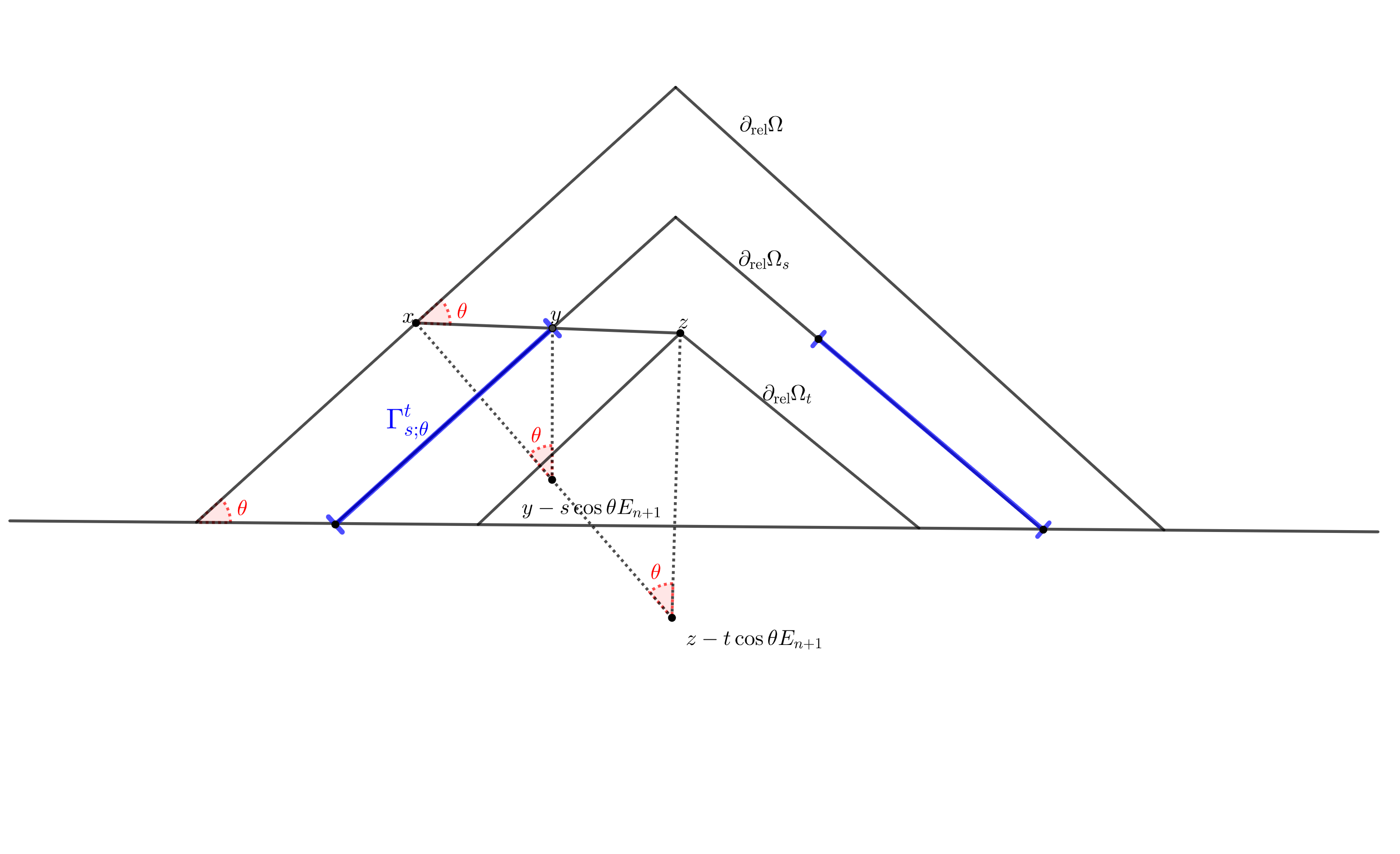
Lemma 3.3.

Given $\theta\in(0,\pi)$, for any nonempty, bounded, relatively open set with finite perimeter $\Omega\subset\overline{\mathbf{R}^{n+1}_{+}}$ and for every $0<s<t<\infty$, let $\Gamma_{s;\theta}^{t}$ be as in Definition 1.5. Then, for any $y\in\Gamma_{s;\theta}^{t}$, it has a unique point projection onto $\partial_{\rm rel}\Omega$ with respect to $\delta_{\theta}$, which reads as $\xi_{\theta}(y)=x$; in other words, $\Gamma_{s;\theta}^{t}\subset{\rm Unp}_{\theta}(\partial_{\rm rel}\Omega)$.

Proof.

By definition, for any $y\in\Gamma_{s;\theta}^{t}$, there exists $x=\gamma_{y}(0)\in\partial_{\rm rel}\Omega$, $z=\gamma_{y}(t)\in\partial_{\rm rel}\Omega_{t}$. Consider the geodesic $\gamma_{y}(r)-r\cos\theta E_{n+1}$ defined on $r\in[0,t]$, by (1.4) there holds

$$\delta(\gamma_{y}(r)-r\cos\theta E_{n+1})=\delta_{\theta}(\gamma_{y}(r))=r\quad\forall r\in[0,t],$$

which means $\gamma_{y}(r)-r\cos\theta E_{n+1}$ is a unit-speed line segment, and it is easy to see the following claim holds.

Claim. $|x-(y-s\cos\theta E_{n+1})|=s,|y-s\cos\theta E_{n+1}-(z-t\cos\theta E_{n+1})|=t-s$.

Now we show that $x$ is uniquely determined by $y$. Since $y\in\partial_{\rm rel}\Omega_{s}$, if there exists $x^{\prime}\neq x\in\partial_{\rm rel}\Omega$ such that $|x^{\prime}-(y-s\cos\theta E_{n+1})|=s$, then by the triangle inequality we have

$$|x^{\prime}-(z-t\cos\theta E_{n+1})|<|x^{\prime}-(y-s\cos\theta E_{n+1})|+|y-z+(t-s)\cos\theta E_{n+1}|=s+t-s=t,$$

contradicts to the fact that $z\in\partial_{\rm rel}\Omega_{t}$. Therefore, we have showed that $x$ is the unique point of $\partial_{\rm rel}\Omega$ nearest to $y$ with respect to $\delta_{\theta}$; that is, $\xi_{\theta}(y)=x$. ∎

Once $0<s<t<\infty$ and $y\in\Gamma_{s;\theta}^{t}$ are fixed, it follows from Lemma 3.3 that the geodesic (constant-speed line segment) $\gamma_{y}:[0,t]\rightarrow\mathbf{R}^{n+1}$ as in Definition 1.5 is unique. Moreover, for the geodesic $\gamma_{y}(r)-r\cos\theta E_{n+1}$ defined on $r\in[0,t]$, we see from the proof of Lemma 3.3 that any point on it has a unique point projection onto $\partial_{\rm rel}\Omega$ with respect to the distance function $\delta$, which reads as

$$\xi(\gamma_{y}(r)-r\cos\theta E_{n+1})=x,\quad\forall r\in[0,t).$$

Equipped with the fact that $\Gamma_{s;\theta}^{t}\subset{\rm Unp}_{\theta}(\partial_{\rm rel}\Omega)$, we can explore the shifted distance function $\delta_{\theta}$ on $\mathbf{R}^{n+1}$ and the unique point projection mapping $\xi_{\theta}$ on $\Gamma_{s;\theta}^{t}$. We collect the fine properties of $\delta_{\theta}$ and $\xi_{\theta}$ as follows.

Lemma 3.4.

Given $\theta\in(0,\pi)$, for any nonempty, bounded, relatively open set with finite perimeter $\Omega\subset\overline{\mathbf{R}^{n+1}_{+}}$, the following statements hold:

1. $\delta_{\theta}$ is a Lipschitz function on $\mathbf{R}^{n+1}$ with Lipschitz constant at most $\frac{1}{1-|\cos\theta|}$, i.e., for any $x,y\in\mathbf{R}^{n+1}$,

   $$|\delta_{\theta}(y)-\delta_{\theta}(x)|\leq\frac{1}{1-|\cos\theta|}|x-y|.$$

2. For $0\leq r_{1}<r_{2}$, and for any $y\in\mathbf{R}^{n+1}$, the strictly inclusion holds:

   $$B_{r_{1}}(y-r_{1}\cos\theta E_{n+1})\subset B_{r_{2}}(y-r_{2}\cos\theta E_{n+1}).$$

3. $N_{\theta}(y):=\nabla\delta_{\theta}(y)$ exists for $\mathcal{L}^{n+1}$-a.e. $y\in\mathbf{R}^{n+1}$. Moreover, when it exists, there holds

   $$\frac{1}{1+|\cos\theta|}\leq|N_{\theta}(y)|\leq\frac{1}{1-|\cos\theta|}.$$ (3.2)

   In particular, as $\theta=\pi/2$, $|N_{\theta}(y)|=1$ when it exists.

4. For $0<s<t$, $\xi_{\theta}$ is continuous on $\Gamma_{s;\theta}^{t}$.

Proof.

(1) We fix any $x,y\in\mathbf{R}^{n+1}$. Since $\partial_{\rm rel}\Omega$ is compact in $\mathbf{R}^{n+1}$, we can take $a\in\partial_{\rm rel}\Omega$ such that $\delta_{\theta}(x)=|a-(x-\delta_{\theta}(x)\cos\theta E_{n+1})|$. We assume without loss of generality that $\delta_{\theta}(y)\geq\delta_{\theta}(x)$, then by the triangle inequality, we find

$$|\delta_{\theta}(y)-\delta_{\theta}(x)|= \delta_{\theta}(y)-\delta_{\theta}(x)$$

$$\leq |a-(y-\delta_{\theta}(y)\cos\theta E_{n+1})|-|a-(x-\delta_{\theta}(x)\cos\theta E_{n+1})|$$

$$\leq |x-y+(\delta_{\theta}(y)-\delta_{\theta}(x))\cos\theta E_{n+1}|$$

$$\leq |x-y|+|\delta_{\theta}(y)-\delta_{\theta}(x)||\cos\theta|,$$

we rearrange this to see

$$|\delta_{\theta}(y)-\delta_{\theta}(x)|\leq\frac{1}{1-|\cos\theta|}|x-y|.$$ (3.3)

This completes the proof of (1).

(2) This amounts to be a simple observation due to the triangle inequality. Indeed, for any $z\in\partial B_{r_{1}}(y-r_{1}\cos\theta E_{n+1})$, if $|z-(y-r_{2}\cos\theta E_{n+1})|\geq r_{2}$, then we have

$${\rm dist}(z,y-r_{1}\cos\theta E_{n+1})+{\rm dist}(y-r_{1}\cos\theta E_{n+1},y-r_{2}\cos\theta E_{n+1})\geq{\rm dist}(z,y-r_{2}\cos\theta E_{n+1}),$$

namely,

$$r_{1}+(r_{2}-r_{1})|\cos\theta|\geq r_{2},$$

which leads to a contradiction since $\theta\in(0,\pi)$ and completes the proof of (2).

(3) By virtue of the Rademacher’s theorem, $\delta_{\theta}$ is differentiable at $\mathcal{L}^{n+1}$-a.e. $y\in\mathbf{R}^{n+1}$. When $N_{\theta}(y)$ exists, we may assume that there exists a unique $x\in\partial_{\rm rel}\Omega$, such that $\delta_{\theta}(y)=|x-(y-\delta_{\theta}(y)\cos\theta E_{n+1})|$.

Claim 1. $\nabla\delta_{\theta}(y)\parallel x-(y-\delta_{\theta}(y)\cos\theta E_{n+1}).$

Indeed, thanks to (1.4), we have the following relation of distance and shifted distance:

$$\delta(y-\delta_{\theta}(y)\cos\theta E_{n+1})=\delta_{\theta}(y).$$ (3.4)

Notice that by virtue of [Fed59, Theorem 4.8 (3)], $\left(\nabla\delta\right)(y-\delta_{\theta}(y)\cos\theta E_{n+1})=\frac{x-(y-\delta_{\theta}(y)\cos\theta E_{n+1})}{\delta_{\theta}(y)}$. Differentiating both sides of (3.4), we get the claim.

Claim 2. For any $0<t\leq 1$, $\delta_{\theta}\left(y+t(x-y)\right)=(1-t)\delta_{\theta}(y)$.

Observe that $y+t(x-y)-(1-t)\delta_{\theta}(y)\cos\theta E_{n+1}=y-\delta_{\theta}(y)\cos\theta E_{n+1}+t\left(x-(y-\delta_{\theta}(y)\cos\theta E_{n+1})\right)$, and trivially we have $|x-{\rm RHS}|=(1-t)\delta_{\theta}(y)$, since ${\rm dist}(x,y-\delta_{\theta}(y)\cos\theta E_{n+1})=\delta_{\theta}(y)$. Therefore, we have: $\delta_{\theta}(y+t(x-y))\leq(1-t)\delta_{\theta}(y)$.

On the other hand, since $1/(1-t)>1$, we know that

$$\bar{B}_{(1-t)\delta_{\theta}(y)}\left(y+t(x-y)-(1-t)\delta_{\theta}(y)\cos\theta E_{n+1}\right)\subset\bar{B}_{\delta_{\theta}(y)}\left(y-\delta_{\theta}(y)\cos\theta E_{n+1}\right)$$

with the only common point $x$, and it follows from (2) that for any $r<(1-t)\delta_{\theta}(y)$, $B_{r}(y+t(x-y)-r\cos\theta E_{n+1})\cap\partial_{\rm rel}\Omega=\varnothing$, which implies $\delta_{\theta}(y+t(x-y))=(1-t)\delta_{\theta}(y)$ and proves the claim.

Now we are ready to carry out the proof of (3.2), we abbreviate $N_{\theta}(y)/|N_{\theta}(y)|$ by $\hat{N}_{\theta}(y)$.

By Claim 1 we know that $x-(y-\delta_{\theta}(y)\cos\theta E_{n+1})=-\delta_{\theta}(y)\hat{N}_{\theta}(y)$, and hence $x-y=-\delta_{\theta}(y)(\hat{N}_{\theta}(y)+\cos\theta E_{n+1})$. Notice that the Taylor expansion of $\delta_{\theta}(y+t(x-y))$ at $y$ gives

$$\delta_{\theta}(y+t(x-y))=\delta_{\theta}(y)+tN_{\theta}(y)\cdot\left(x-y\right)+o(t),$$

which, by Claim 2 and the above observation, reads as

$$-t\delta_{\theta}(y)=tN_{\theta}(y)\cdot\left(-\delta_{\theta}(y)\left(\hat{N}_{\theta}(y)+\cos\theta E_{n+1}\right)\right)+o(t),$$

sending $t\searrow 0^{+}$ and rearranging, we thus find

$$|N_{\theta}(y)|=\frac{1}{1+\cos\theta\hat{N}_{\theta}(y)\cdot E_{n+1}},$$ (3.5)

(3.2) follows easily.

For (4), suppose on the contrary that there exists some $\epsilon>0$ and a sequence of points $\{y_{i}\}_{i=1}^{\infty}\subset\Gamma_{s;\theta}^{t}$, converges to $y\in\Gamma_{s;\theta}^{t}$, such that $|\xi_{\theta}(y)-\xi_{\theta}(y_{i})|\geq\epsilon$ for every large $i$.

By definition, for each $i$, we have, for $i$ large, there holds

$$|\xi_{\theta}(y_{i})-(y_{i}-s\cos\theta E_{n+1})|=\delta_{\theta}(y_{i})=s.$$ (3.6)

Using the triangle inequality and the fact that $y_{i}$ converges to $y$, we find

$$|\xi_{\theta}(y_{i})-(y-s\cos\theta E_{n+1})|\leq |\xi_{\theta}(y_{i})-(y_{i}-s\cos\theta E_{n+1})|+|y_{i}-y|$$

$$= s+|y_{i}-y|<s+\epsilon.$$

This means, all the points $\{\xi_{\theta}(y_{i})\}_{i}$ are lying in $\partial_{\rm rel}\Omega\cap B_{s+\epsilon}(y-s\cos\theta E_{n+1})$, which is a bounded subset of the compact set $\partial_{\rm rel}\Omega$, and hence by passing to a subsequence, we can assume that $\{\xi_{\theta}(y_{i})\}_{i}$ converges to some point $x\in\partial_{\rm rel}\Omega$. But then, since $\delta_{\theta}$ is continuous, we have

$$s=\delta_{\theta}(y)=\lim_{i\rightarrow\infty}\delta_{\theta}(y_{i})=\lim_{i\rightarrow\infty}|\xi_{\theta}(y_{i})-(y_{i}-s\cos\theta E_{n+1})|=|x-(y-s\cos\theta E_{n+1})|,$$

which implies that $x=\xi_{\theta}(y)$ since we have proved that $y\in\Gamma_{s;\theta}^{t}\subset{\rm Unp}_{\theta}(\partial_{\rm rel}\Omega)$ in Lemma 3.3. However, this contradicts to the assumption that

$$|x-\xi_{\theta}(y)|=\lim_{i\rightarrow\infty}|\xi_{\theta}(y_{i})-\xi_{\theta}(y)|\geq\epsilon,$$

and hence completes the proof. ∎

Remark 3.5.

When $\Omega$ is contained in a Euclidean space, similar results are included in [Fed59, 4.8(1)(2)(3)(4)].

With the help of Lemma 3.3 and Lemma 3.4, we can fully explore the fine properties of $\Gamma_{s;\theta}^{t}$ and $\Gamma_{s;\theta}^{+}$, which are well understood in the Euclidean case, see [DM19, Theorem1].

Proposition 3.6.

Given $\theta\in(0,\pi)$. For any nonempty, bounded, relatively open set with finite perimeter $\Omega\subset\overline{\mathbf{R}^{n+1}_{+}}$ and for every $0<s<t<\infty$, there holds

1. For $s<t_{1}<t_{2}$, $\Gamma_{s;\theta}^{t_{2}}\subset\Gamma_{s;\theta}^{t_{1}}$. In particular, $\Gamma_{s;\theta}^{+}=\lim_{t\rightarrow s^{+}}\Gamma_{s;\theta}^{t}$.

2. $\Gamma_{s;\theta}^{t}$ is a compact set in $\overline{\mathbf{R}^{n+1}_{+}}$.

3. At any $y\in\Gamma_{s;\theta}^{t}$, $\Gamma_{s;\theta}^{t}$ is bounded by two mutually tangent balls in $\mathbf{R}^{n+1}$ with radii $s$ and $t-s$.

4. $\delta_{\theta}$ is differentiable at every $y\in\Gamma_{s;\theta}^{t}$.

Proof.

(1) The first part of the statement follows easily from the definition of $\Gamma_{s;\theta}^{t}$, while by virtue of the inclusion, it is apparent that $\Gamma_{s;\theta}^{+}=\lim_{t\rightarrow s^{+}}\Gamma_{s;\theta}^{t}$.

(2) It suffice to prove that $\Gamma_{s;\theta}^{t}$ is a closed set, i.e., if a sequence of points $\{y_{i}\}_{i=1}^{\infty}\subset\Gamma_{s;\theta}^{t}$ converges to $y$, then it must be that $y\in\Gamma_{s;\theta}^{t}$.

By definition of $\Gamma_{s;\theta}^{t}$, for each $y_{i}$, there exists corresponding points $x_{i}\in\partial_{\rm rel}\Omega,z_{i}\in\partial_{\rm rel}\Omega_{t}$. By Lemma 3.4, $\xi_{\theta}$ is continuous on $\Gamma_{s}^{t}$, and hence we have: $\{x_{i}\}_{i=1}^{\infty}$ is a Cauchy sequence in $\partial_{\rm rel}\Omega$. Notice that $\partial_{\rm rel}\Omega$ is closed in $\mathbf{R}^{n+1}$, and hence $\{x_{i}\}_{i=1}^{\infty}$ converges to some $x\in\partial_{\rm rel}\Omega$. Similarly, $\{z_{i}\}_{i=1}^{\infty}$ converges to some $z\in\partial_{\rm rel}\Omega_{t}$.

By continuity, we have

$$\delta_{\theta}(y)=\lim_{i\rightarrow\infty}\delta_{\theta}(y_{i})=s,\quad|x-(y-s\cos\theta E_{n+1})|=\lim_{i\rightarrow\infty}|\xi_{\theta}(y_{i})-(y_{i}-s\cos\theta E_{n+1})|=s.$$

Similarly, we deduce that $|y-s\cos\theta E_{n+1}-(z-t\cos\theta E_{n+1})|=t-s$. By using the triangle inequality again, we find

$$t=\delta_{\theta}(z)\leq |x-(z-t\cos\theta E_{n+1})|$$

$$\leq |x-(y-s\cos\theta E_{n+1})|+|y-z+(t-s)\cos\theta E_{n+1}|=t,$$

it is easy to see that the line segment joining $x$ and $z-t\cos\theta E_{n+1}$ must contain $y-s\cos\theta E_{n+1}$, and hence one may verify that $y\in\Gamma_{s;\theta}^{t}$ by definition, which completes the proof of (2).

(3) can be deduced from the definition of $\Gamma_{s;\theta}^{t}$ and Lemma 3.3. Indeed, it is easy to see that for every $y\in\Gamma_{s;\theta}^{t}$,

$$\{y-s\cos\theta E_{n+1}\}=\partial B_{t-s}(z-t\cos\theta E_{n+1})\cap\partial B_{s}(x),$$ (3.7)

and hence $\Gamma^{t}_{s;\theta}-s\cos\theta E_{n+1}$ is trapped between $B_{t-s}(z-t\cos\theta E_{n+1})$ and $B_{s}(x)$ at $y-s\cos\theta E_{n+1}$. This in turn implies that $\Gamma^{t}_{s;\theta}$ is trapped between two mutually tangent balls with radii $s$ and $t-s$ at every of its points.

(4) is a direct consequence of the fact that $y\in\Gamma_{s;\theta}^{t}\subset{\rm Unp}_{\theta}(\partial_{\rm rel}\Omega)$, which we proved in Lemma 3.3. ∎

3.2. $C^{1,1}$-rectifiability theorem and its consequences

Proof of Theorem 3.1.

We follow closely the proof in [DM19, Proof of Theorem 1: Step 1] with modifications to our shifted distance function $\delta_{\theta}$. Recall that we denote by $N_{\theta}(y)$ the gradient of $\delta_{\theta}$ at $y$, which exists at every $y\in\Gamma_{s;\theta}^{t}$ thanks to Proposition 3.6(4), and we denote the normalized vector $N_{\theta}(y)/|N_{\theta}(y)|$ simply by $\hat{N}_{\theta}(y)$.

Step 1. $C^{1}$-rectifiability of $\Gamma_{s;\theta}^{t}$.

First we estimate $\left|N_{\theta}(y)\cdot(y^{\prime}-y)\right|$ for any $y,y^{\prime}\in\Gamma_{s;\theta}^{t}$. By virtue of Lemma 3.4(3) and Proposition 3.6, we get an explicit expression of $N_{\theta}(y)$ by $x,y,z$. Indeed, by virtue of Claim 1 in the proof of Lemma 3.4(3), we find

$$\hat{N}_{\theta}(y)=\frac{-x+(z-t\cos\theta E_{n+1})}{|-x+(z-t\cos\theta E_{n+1})|}.$$ (3.8)

This, together with Claim 2 in the proof of Lemma 3.4(3), implies the following fact: for any $y\in\Gamma_{s;\theta}^{t}$, and for $r\in[-s,t-s]$, there holds

$$y-s\cos\theta E_{n+1}+r\hat{N}_{\theta}(y)\in\partial_{\rm rel}\Omega_{s+r}-(s+r)\cos\theta E_{n+1},$$ (3.9)

here we adopt the convention that $\partial_{\rm rel}\Omega_{0}=\partial_{\rm rel}\Omega$. We rearrange this to see

$$y+r(\hat{N}_{\theta}(y)+\cos\theta E_{n+1})\in\partial_{\rm rel}\Omega_{s+r}.$$ (3.10)

Using (3.10) and recalling (1.4), for $y,y^{\prime}\in\Gamma_{s;\theta}^{t}$, we have

$$s^{2}\leq |y-s(\hat{N}_{\theta}(y)+\cos\theta E_{n+1})-(y^{\prime}-s\cos\theta E_{n+1})|^{2}$$

$$= s^{2}-2s\hat{N}_{\theta}(y)\cdot(y-y^{\prime})+|y-y^{\prime}|^{2},$$ (3.11)

and also

$$(t-s)^{2}\leq |\left(y+(t-s)(\hat{N}_{\theta}(y)+\cos\theta E_{n+1})-t\cos\theta E_{n+1}\right)-(y^{\prime}-s\cos\theta E_{n+1})|^{2}$$

$$= |y+(t-s)\hat{N}_{\theta}(y)-y^{\prime}|^{2}=(t-s)^{2}+2(t-s)\hat{N}_{\theta}(y)\cdot(y-y^{\prime})+|y-y^{\prime}|^{2}.$$ (3.12)

Combining these facts and using (3.2), we obtain the estimate

$$|N_{\theta}(y)\cdot(y^{\prime}-y)|\leq |N_{\theta}(y)|\max\{\frac{1}{s},\frac{1}{t-s}\}\frac{|y-y^{\prime}|^{2}}{2}$$

$$\leq \max\{\frac{1}{s},\frac{1}{t-s}\}\frac{|y-y^{\prime}|^{2}}{2(1-|\cos\theta|)}\quad\text{for all }y,y^{\prime}\in\Gamma_{s;\theta}^{t}.$$ (3.13)

By Proposition 3.6, $N_{\theta}$ is continuous on $\Gamma_{s;\theta}^{t}$, and hence we have the pair $(\delta_{\theta},N_{\theta})\in C^{0}(\Gamma_{s;\theta}^{t};\mathbf{R}\times\mathbf{R}^{n+1})$, satisfying the key estimate (3.2). Observe that

$$\limsup_{\epsilon\rightarrow 0^{+}}\{\frac{|\delta_{\theta}(y^{\prime})-\delta_{\theta}(y)-N_{\theta}(y)\cdot(y^{\prime}-y)|}{|y^{\prime}-y|}:0<|y^{\prime}-y|\leq\epsilon,\quad y^{\prime},y\in\Gamma_{s;\theta}^{t}\}$$

$$\leq \limsup_{\epsilon\rightarrow 0^{+}}\left\{\frac{\max\{\frac{1}{2(t-s)},\frac{1}{2s}\}|y-y^{\prime}|^{2}}{\left(1-|\cos\theta|\right)|y^{\prime}-y|}:0<|y^{\prime}-y|\leq\epsilon,\quad y^{\prime},y\in\Gamma_{s;\theta}^{t}\right\}=0,$$ (3.14)

where in the inequality we used the fact that $\delta_{\theta}(y^{\prime})=\delta_{\theta}(y)=s$ and (3.2). In particular, with this in force, we can use the $C^{1}$-Whitney’s extension theorem to find that there exists $\phi_{\theta}\in C^{1}(\mathbf{R}^{n+1})$ such that $(\phi_{\theta},\nabla\phi_{\theta})=(\delta_{\theta},N_{\theta})$ on $\Gamma_{s;\theta}^{t}$. Moreover, by (3.8) we know that $N_{\theta}(y)\neq 0$, and hence we can use the $C^{1}$-Implicit function theorem for $\phi_{\theta}$ to find: for every $y\in\Gamma_{s;\theta}^{t}$, there exists an open set $U\subset\mathbf{R}^{n}$, and a $C^{1}$-function $\psi:U\rightarrow\mathbf{R}^{1}$, such that $\Gamma_{s;\theta}^{t}\subset(x^{\prime},\psi(x^{\prime}))$ on $U$, i.e., $\Gamma_{s;\theta}^{t}$ lies in the $C^{1}$-image of $\Psi:U\subset\mathbf{R}^{n}\rightarrow\mathbf{R}^{n+1}$, given by $\Psi(x^{\prime})=(x^{\prime},\psi(x^{\prime}))$. On the other hand, using the coarea formula and invoking (3.2), we obtain

$$\frac{|\Omega|}{1-|\cos\theta|}\geq\int_{\Omega}|\nabla\delta_{\theta}|{\rm d}\mathcal{L}^{n+1}=\int_{0}^{\infty}\mathcal{H}^{n}(\partial_{\rm rel}\Omega_{s}){\rm d}s,$$ (3.15)

since $\Omega$ is bounded, this implies, for a.e. $s>0$, $\mathcal{H}^{n}(\partial_{\rm rel}\Omega_{s})<\infty$, it follows that $\mathcal{H}^{n}(\Gamma_{s;\theta}^{t})<\infty$ for a.e. $s>0$. In particular, these facts yield the $\mathcal{H}^{n}$-rectifiability of $\Gamma_{s;\theta}^{t}$.

Step 2. $N_{\theta}$ is tangentially differentiable along $\Gamma_{s;\theta}^{t}$ at $\mathcal{H}^{n}$-a.e. $y\in\Gamma_{s;\theta}^{t}$.

As presented in [DM19], the key point of this step is to show that $N_{\theta}$ is Locally Lipschitz on $\Gamma_{s;\theta}^{t}$. Indeed, we will show that for any $\Gamma_{s;\theta}^{t}$ having finite $\mathcal{H}^{n}$-measure, it can be covered, up to a $\mathcal{H}^{n}$-negligible set, by compact sets $\{\mathcal{U}_{j}\}_{j\in\mathbb{N}}$, such that $N_{\theta}\mid_{\mathcal{U}_{j}}$ is Lipschitz.

We first construct $\{\mathcal{U}_{j}\}$, let $\mathcal{C}(N,\rho)=\{z+hN:z\in N^{\perp},|z|<\rho,|h|<\rho\}$ denote the open cylinder in $\mathbf{R}^{n+1}$, centered at the origin with axis along $N\in\mathbf{S}^{n}$, radius $\rho>0$ and height $2\rho$. By Proposition 3.6 and the $C^{1}$-rectifiability of $\Gamma_{s;\theta}^{t}$, we know that $\Gamma_{s;\theta}^{t}$ admits an approximate tangent plane at $\mathcal{H}^{n}$-a.e. of its points and this plane is then exactly $\left\{\hat{N}_{\theta}(y)\right\}^{\perp}$, which is a $n$-dimensional affine plane in $\mathbf{R}^{n+1}$, i.e.,

$$T_{y}\Gamma_{s;\theta}^{t}=\left\{\hat{N}_{\theta}(y)\right\}^{\perp}\quad\text{for }\mathcal{H}^{n}\text{-a.e. }y\in\Gamma_{s;\theta}^{t}.$$

By [Mag12, Theorem 10.2] and notice that for any fixed $\rho$, there exists $0<\rho_{1}<\rho_{2}$ such that $B_{\rho_{1}}\subset\mathcal{C}(\hat{N}_{\theta}(y),\rho)\subset B_{\rho_{2}}$, we have

$$\lim_{\rho\rightarrow 0^{+}}\frac{\mathcal{H}^{n}\left(\Gamma_{s;\theta}^{t}\cap\left(y+\mathcal{C}\left(\hat{N}_{\theta}\left(y\right),\rho\right)\right)\right)}{\omega_{n}\rho^{n}}=1,\quad\text{for }\mathcal{H}^{n}\text{-a.e. }y\in\Gamma_{s;\theta}^{t}.$$

For a sequence $\{\rho_{j}\}_{j\in\mathbb{N}}$ such that $\rho_{j}\rightarrow 0$ as $j\rightarrow\infty$, we set

$$f_{j}(y):=\frac{\mathcal{H}^{n}\left(\Gamma_{s;\theta}^{t}\cap\left(y+\mathcal{C}\left(\hat{N}_{\theta}\left(y\right),\rho_{j}\right)\right)\right)}{\omega_{n}\rho_{j}^{n}},$$

then $f_{j}\rightarrow 1$ for $\mathcal{H}^{n}$-a.e. $y\in\Gamma_{s;\theta}^{t}$. By Egoroff’s theorem and [EG15, Lemma 1.1], there exists a compact set $\mathcal{U}_{1}\subset\Gamma_{s;\theta}^{t}$ such that $f_{j}\rightarrow 1$ uniformly on $\mathcal{U}_{1}$ and $\mathcal{H}^{n}(\Gamma_{s;\theta}^{t}\setminus\mathcal{U}_{1})<\frac{1}{2}\mathcal{H}^{n}(\Gamma_{s;\theta}^{t})$. For $\Gamma_{s;\theta}^{t}\setminus\mathcal{U}_{1}$, we can use Egoroff’s theorem again to find a compact set $\mathcal{U}_{2}\subset\Gamma_{s;\theta}^{t}\setminus\mathcal{U}_{1}$ such that $f_{j}\rightarrow 1$ uniformly on $\mathcal{U}_{2}$ and $\mathcal{H}^{n}\left(\Gamma_{s;\theta}^{t}\setminus\left(\mathcal{U}_{1}\cup\mathcal{U}_{2}\right)\right)<\frac{1}{2^{2}}\mathcal{H}^{n}(\Gamma_{s;\theta}^{t})$. Using an inductive argument, we obtain a sequence of compact sets $\left\{\mathcal{U}_{j}\right\}_{j=1}^{\infty}$ such that $\mathcal{H}^{n}(\Gamma_{s;\theta}^{t}\setminus\bigcup_{j=1}^{\infty}\mathcal{U}_{j})=0$ with $f_{j}\rightarrow 1$ uniformly on each $\mathcal{U}_{j}$. Consequently, we have

$$\mu_{j}^{\ast}(\rho):=\sup_{y\in\mathcal{U}_{j}}\left|1-\frac{\mathcal{H}^{n}\left(\Gamma_{s;\theta}^{t}\cap(y+\mathcal{C}(\hat{N}_{\theta}(y),\rho)\right)}{\omega_{n}\rho^{n}}\right|\rightarrow 0\quad\text{as }\rho\rightarrow 0^{+}.$$ (3.16)

This shows that $\Gamma_{s;\theta}^{t}$ can be covered by a countable union of compact sets, up to a $\mathcal{H}^{n}$-negligible set.

Fix any $y\in\mathcal{U}_{j}\subset\Gamma_{s;\theta}^{t}$, we know from the $C^{1}$-Implicit function theorem that $\mathcal{U}_{j}\subset\Gamma_{s;\theta}^{t}$ is the graph of a $C^{1}$-function $\psi_{j}(\cdot):\mathbf{R}^{n}\rightarrow\mathbf{R}^{1}$ in a neighborhood of $y$. Therefore, up to further subdivision of $\mathcal{U}_{j}$, we may assume that each $\mathcal{U}_{j}$ satisfies: for each $y\in\mathcal{U}_{j}$, there exists

$$\psi_{j}\in C^{1}(\{\hat{N}_{\theta}(y)\}^{\perp}),\quad\psi_{j}(0)=0,\quad\nabla\psi_{j}(0)=0,\quad||\nabla\psi_{j}||_{C^{0}(\{\hat{N}_{\theta}(y)\}^{\perp})}\leq 1,$$ (3.17)

such that, if $\mathcal{U}_{j}^{\prime}$ denotes the projection of $\mathcal{U}_{j}$ on $\{\hat{N}_{\theta}(y)\}^{\perp}\cap\{|z|<\rho_{j}\}$, then

$$\mathcal{U}_{j}\cap(y+\mathcal{C}(\hat{N}_{\theta}(y),\rho_{j}))=\Gamma_{s;\theta}^{t}\cap(y+\mathcal{C}(\hat{N}_{\theta}(y),\rho_{j}))=y+\{z+\psi_{j}(z)\hat{N}_{\theta}(y):z\in\mathcal{U}_{j}^{\prime}\},$$ (3.18)

here $\rho_{j}$, $\psi_{j}$ depend on the choice of the point $y\in\mathcal{U}_{j}$. Moreover, if we set

$$\mu_{j}(\rho):=\max\left\{\mu^{\ast}_{j}(\rho),\max_{|z|\leq\rho}|\nabla\psi_{j}(z)|\right\},\quad\rho\in(0,\rho_{j}],$$ (3.19)

then $\mu_{j}(\rho)\rightarrow 0$ as $\rho\rightarrow 0^{+}$ by (3.16) and the continuity of $\nabla\psi_{j}$. This completes the construction of the covering $\{\mathcal{U}_{j}\}_{j\in\mathbb{N}}$.

To proceed, we need to show that $N_{\theta}$ is Lipschitz on each $\mathcal{U}_{j}$, i.e., for any $y_{1},y_{2}\in\mathcal{U}_{j}$, there exists $C_{j}>0$ for each $j$, such that

$$|N_{\theta}(y_{1})-N_{\theta}(y_{2})|\leq C_{j}|y_{1}-y_{2}|.$$ (3.20)

Since $\mathcal{U}_{j}$ can be written as a $C^{1}$-graph, with Proposition 3.6(3), (3.2) , Lemma 3.4(3) and (3.19) in force, we can adopt exactly the same approach in [DM19, (3-16)] to find

$$|\hat{N}_{\theta}(y_{1})-\hat{N}_{\theta}(y_{2})|\leq\tilde{C}_{j}|y_{1}-y_{2}|.$$ (3.21)

To see that (3.20) holds, we use the triangle inequality to obtain

$$|N_{\theta}(y_{1})-N_{\theta}(y_{2})|\leq|N_{\theta}(y_{1})\Big{|}|\hat{N}_{\theta}(y_{1})-\hat{N}_{\theta}(y_{2})\Big{|}+\Big{|}\left|N_{\theta}(y_{1})\right|-\left|N_{\theta}(y_{2})\right|\Big{|},$$

invoking (3.5), we find

$$\Big{|}\left|N_{\theta}(y_{1})\right|-\left|N_{\theta}(y_{2})\right|\Big{|}= \frac{\left|\cos\theta\left(\hat{N}_{\theta}(y_{2})-\hat{N}_{\theta}(y_{1})\right)\cdot E_{n+1}\right|}{\left(1+\cos\theta\hat{N}_{\theta}(y_{1})\cdot E_{n+1}\right)\left(1+\cos\theta\hat{N}_{\theta}(y_{2})\cdot E_{n+1}\right)}$$

$$\leq \frac{|\cos\theta|}{\left(1-|\cos\theta|\right)^{2}}\left|\hat{N}_{\theta}(y_{1})-\hat{N}_{\theta}(y_{2})\right|.$$

This, together with the estimate (3.2) and also (3.21), gives exactly (3.20).

Recall that $\Gamma_{s;\theta}^{t}$ can be covered by $\{\mathcal{U}_{j}\}$, up to a $\mathcal{H}^{n}$-negligible set, and hence by virtue of Rademacher’s theorem, $N_{\theta}$ is tangentially differentiable along $\Gamma_{s;\theta}^{t}$ at $\mathcal{H}^{n}$-a.e. $y\in\Gamma_{s;\theta}^{t}$.

Conclusion of the proof. $C^{1,1}$-rectifiability of $\Gamma_{s;\theta}^{+}$.

By (3.2) and (3.20), on each $\mathcal{U}_{j}$, we can use the Whitney-Glaser extension theorem to see that there exists $\phi_{\theta}\in C^{1,1}(\mathbf{R}^{n+1})$ such that $(\delta_{\theta},N_{\theta})=(\phi_{\theta},\nabla\phi_{\theta})$ on $\mathcal{U}_{j}$. Then, by the ${C^{1,1}}$-Implicit function theorem, for each $y\in\mathcal{U}_{j}$, there exists $\psi_{j}\in C^{1,1}(\left\{\hat{N}_{\theta}(y)\right\}^{\perp})$ satisfying (3.17) and (3.18), which completes the proof.

∎

Proposition 3.7.

Given $\theta\in(0,\pi)$, let $\Omega$ be a nonempty, bounded, relatively open set with finite perimeter in $\overline{\mathbf{R}^{n+1}_{+}}$, for every $0<t<\infty$, and for a.e. $0<s<t$, there holds

1. $N_{\theta}$ is tangentially differentiable along $\Gamma_{s;\theta}^{t}$ at $\mathcal{H}^{n}$-a.e. $y\in\Gamma_{s;\theta}^{t}$, with

   $$\begin{cases}\nabla^{\Gamma_{s;\theta}^{t}}\hat{N}_{\theta}(y)=-\sum_{i=1}^{n}(\kappa_{s;\theta}^{t})_{i}(y)\tau_{i}(y)\otimes\tau_{i}(y),\\ -1/s\leq(\kappa_{s;\theta}^{t})_{i}(y)\leq 1/(t-s),\end{cases}$$ (3.22)

   where $\left\{\left(\kappa_{s;\theta}^{t}\right)_{i}(y)\right\}_{i=1}^{n}$ denote the principal curvatures of $\hat{N}_{\theta}$ along $\Gamma_{s;\theta}^{t}$ at $y$ which are indexed in increasing order.

2. Letting $\Omega^{\star}_{\theta}:=\bigcup_{s>0}\Gamma_{s;\theta}^{+}$, then $|\Omega\Delta\Omega^{\star}_{\theta}|=0.$

3. For every $r<s<t$, the map $g_{r;\theta}:\Gamma_{s;\theta}^{t}\rightarrow\Gamma_{s-r;\theta}^{t}$, given by $g_{r;\theta}(y)=y-r(\hat{N}_{\theta}(y)+\cos\theta E_{n+1})$ for $y\in\Gamma_{s;\theta}^{t}$, is a bijection from $\Gamma_{s;\theta}^{t}$ to $\Gamma_{s-r;\theta}^{t}$ and is Lipschitz when restricted to each $\mathcal{U}_{j}$, with

   $$J^{\Gamma_{s;\theta}^{t}}g_{r;\theta}(y)=\prod_{i=1}^{n}\left(1+r(\kappa_{s;\theta})_{i}(y)\right),\quad(\kappa^{t}_{s-r;\theta})_{i}(g_{r;\theta}(y))=\frac{(\kappa^{t}_{s;\theta})_{i}(y)}{1+r(\kappa^{t}_{s;\theta})_{i}(y)},$$ (3.23)

   for $\mathcal{H}^{n}$-a.e. $y\in\Gamma_{s}^{t}$.

Proof.

(1) Consider those $\Gamma_{s;\theta}^{t}$ resulting from the conclusion of Theorem 3.1. Recall that we have proved: $N_{\theta}$ is tangentially differentiable along ${\Gamma_{s;\theta}^{t}}$ at $\mathcal{H}^{n}$-a.e. $y\in\Gamma_{s;\theta}^{t}$ in Theorem 3.1, which is done by constructing a sequence of compact sets $\mathcal{U}_{j}$, such that $\mathcal{H}^{n}(\Gamma_{s}^{t}\setminus\bigcup_{j=1}^{\infty}\mathcal{U}_{j})=0$, where each $\mathcal{U}_{j}$ is proved to be contained in the graph of some $C^{1,1}$-function, on which $N_{\theta}$ is Lipschitz, see (3.20).

By virtue of Lemma 2.2, to study the tangential gradient of $\hat{N}_{\theta}$ along $\Gamma_{s;\theta}^{t}$, it suffice to work on each $\mathcal{U}_{j}$ (see (3.17) and (3.18) for the construction of $\mathcal{U}_{j}$).

To proceed, for any $y\in\mathcal{U}_{j}$, we consider a natural Lipschitz extension of $\hat{N}_{\theta}$, from $\mathcal{U}_{j}\cap\left(y+\mathcal{C}(\hat{N}_{\theta}(y),\rho)\right)$ to $y+\mathcal{C}(\hat{N}_{\theta}(y),\rho)$, denoted by $\hat{N}_{\theta\ast}$ and is given by

$$\hat{N}_{\theta\ast}(y+z+h\hat{N}_{\theta}(y))=\hat{N}_{\theta}(y+z),\quad\forall z\in\{\hat{N}_{\theta}(y)\}^{\perp},|z|,h<\rho_{j},$$ (3.24)

where $\hat{N}_{\theta}(y+z)$ is just the upwards pointing unit normal of the graph $(x^{\prime},\psi_{j}(x^{\prime}))$ at $y+z\in\mathcal{U}^{\prime}_{j}$. With such Lipschitz extension and recalling Proposition 3.6(3), we can follow the classical argument in [DM19, Theorem1, Step1] to conclude (1).

(2) We divide the proof into 2 steps.

Step 1. For every $0<s<t<\infty$, there holds

$$\mathcal{H}^{n}(\partial_{\rm rel}\Omega_{t})\leq(t/s)^{n}\mathcal{H}^{n}(\Gamma_{s;\theta}^{t}).$$ (3.25)

Indeed, for $r\in[-s,t-s]$, we consider the map

$$f_{r;\theta}:\Gamma_{s;\theta}^{t}\rightarrow\partial_{\rm rel}\Omega_{s+r},\quad f_{r;\theta}(y)=y+r(\hat{N}_{\theta}(y)+\cos\theta E_{n+1}).$$ (3.26)

To see that $f_{r;\theta}(y)\in\partial_{\rm rel}\Omega_{s+r}$, we invoke (3.10). Notice that by the definition of $\Gamma_{s;\theta}^{t}$, the map $f_{t-s;\theta}$ is surjective; that is, $\partial_{\rm rel}\Omega_{t}=f_{t-s;\theta}(\Gamma_{s;\theta}^{t})$. Consequently, we can use the area formula (2.1) to see that

$$\mathcal{H}^{n}(\partial_{\rm rel}\Omega_{t})=\mathcal{H}^{n}(f_{t-s;\theta}(\Gamma_{s;\theta}^{t}))\leq\int_{f_{t-s;\theta}(\Gamma_{s;\theta}^{t})}\mathcal{H}^{0}(f_{t-s;\theta}^{-1}(z)){\rm d}\mathcal{H}^{n}(z)=\int_{\Gamma_{s;\theta}^{t}}{\rm J}^{\Gamma_{s;\theta}^{t}}f_{t-s}{\rm d}\mathcal{H}^{n},$$ (3.27)

where ${\rm J}^{\Gamma_{s;\theta}^{t}}f_{t-s;\theta}$ denotes the tangential Jacobian of $f_{t-s;\theta}$ along $\Gamma_{s;\theta}^{t}$. By virtue of (1), a simple computation then yields

$${\rm J}^{\Gamma_{s;\theta}^{t}}f_{t-s;\theta}=\prod_{i=1}^{n}(1-(t-s)(\kappa_{s;\theta}^{t})_{i})\leq(1+\frac{t-s}{s})^{n}=(\frac{t}{s})^{n}\quad\mathcal{H}^{n}\text{-}a.e.\text{ on }\Gamma_{s;\theta}^{t},$$

where we have used (3.22) for the inequality. In particular, this completes the step.

Step 2. $|\Omega\Delta\Omega^{\star}_{\theta}|=0$.

We first apply the coarea formula to find

$$\frac{|\Omega\Delta\Omega^{\star}_{\theta}|}{1+|\cos\theta|}\leq\int_{\Omega\Delta\Omega^{\star}_{\theta}}|\nabla\delta_{\theta}|{\rm d}\mathcal{L}^{n+1}=\int_{0}^{\infty}\mathcal{H}^{n}\left((\Omega\Delta\Omega^{\star}_{\theta})\cap\partial_{\rm rel}\Omega_{s}\right){\rm d}s=\int_{0}^{\infty}\mathcal{H}^{n}(\partial_{\rm rel}\Omega_{s}\setminus\Gamma_{s;\theta}^{+}){\rm d}s,$$ (3.28)

where we have used (3.2) for the first inequality; the fact that $\Gamma_{s;\theta}^{+}\subset\partial_{\rm rel}\Omega_{s}$ for the last equality.

Claim. For a.e. $s>0$, there holds

$$\mathcal{H}^{n}(\Gamma_{s;\theta}^{+})=\mathcal{H}^{n}(\partial_{\rm rel}\Omega_{s}).$$ (3.29)

If the claim holds, we immediately deduce that $|\Omega\Delta\Omega^{\star}_{\theta}|=0$ by virtue of (3.28), which proves (2). Now we prove the claim, using the coarea formula and the estimate (3.2) again, we find: for every $0<s<t<\infty$,

$$\int_{s}^{t}\mathcal{H}^{n}(\partial_{\rm rel}\Omega_{r}){\rm d}r=\int_{\Omega_{s}\setminus\Omega_{t}}|\nabla\delta_{\theta}|{\rm d}\mathcal{L}^{n+1}\leq\frac{|\Omega_{s}\setminus\Omega_{t}|}{1-|\cos\theta|}\leq\frac{|\Omega|}{1-|\cos\theta|}<\infty,$$

which implies that the function $\mathcal{H}^{n}(\partial\Omega_{r})$ is integrable on any $[s,t]\subset\mathbf{R}^{+}$. Therefore, we can exploit the Lebesgue-Besicovitch Differentiation Theorem (see e.g., [EG15, Theorem 1.32]) to obtain

$$\mathcal{H}^{n}(\partial_{\rm rel}\Omega_{s})=\lim_{\epsilon\rightarrow 0^{+}}\frac{1}{2\epsilon}\int_{-\epsilon}^{\epsilon}\mathcal{H}^{n}(\partial_{\rm rel}\Omega_{s+r}){\rm d}r\quad\text{for a.e. }s>0,$$ (3.30)

whereby (3.25) and Proposition 3.6(1),

$$\frac{1}{2\epsilon}\int_{-\epsilon}^{\epsilon}\mathcal{H}^{n}(\partial_{\rm rel}\Omega_{s+r}){\rm d}r\leq\frac{1}{2\epsilon}\int_{-\epsilon}^{\epsilon}(1+r/s)^{n}\mathcal{H}^{n}(\Gamma_{s;\theta}^{s+r}){\rm d}r\leq(1+\epsilon/s)^{n}\mathcal{H}^{n}(\Gamma_{s;\theta}^{+}).$$

Since $\Gamma_{s;\theta}^{+}\subset\partial_{\rm rel}\Omega_{s}$, this proves (3.29) and hence (2).

(3) By virtue of (3.10), $g_{r;\theta}$ is a bijection between $\Gamma_{s;\theta}^{t}$ and $\Gamma_{s-r;\theta}^{t}$ for every $r\in(0,s)$ and $t>0$. We note that if $y$ is a point of tangential differentiability of $\hat{N}_{\theta}$ along $\Gamma_{s;\theta}^{t}$, then $g_{r;\theta}(y)$ is a point of tangential differentiability of $N_{\theta}$ along $\Gamma_{s-r;\theta}^{t}$. Indeed, by virtue of Claim 1 in the proof of Lemma 3.4(3), we have

$$\hat{N}_{\theta}(y)=\hat{N}_{\theta}(g_{r;\theta}(y))=\hat{N}_{\theta}\left(y-r(\hat{N}_{\theta}(y)+\cos\theta E_{n+1})\right)\quad\text{for all }y\in\Gamma_{s;\theta}^{t},$$ (3.31)

so that if $y$ is a point of tangential differentiability of $N_{\theta}$ along $\Gamma_{s;\theta}^{t}$ and $\tau\in T_{y}\Gamma_{s;\theta}^{t}$, then $\tau\in T_{g_{r;\theta}(y)}\Gamma_{s-r;\theta}^{t}$ and

$$(\nabla^{\Gamma_{s;\theta}^{t}}\hat{N}_{\theta})_{y}[\tau]=(\nabla^{\Gamma_{s-r;\theta}^{t}}\hat{N}_{\theta})_{g_{r;\theta}(y)}\left[\tau-r(\nabla^{\Gamma_{s;\theta}^{t}}\hat{N}_{\theta})_{y}[\tau]\right].$$

Consider the eigenvectors $\{\tau_{i}(y)\}_{i=1}^{n}$ of $\hat{N}_{\theta}$ in (3.22), we find

$$-(\kappa_{s;\theta}^{t})_{i}(y)\tau_{i}(y)=(1+r(\kappa_{s;\theta}^{t})_{i}(y))(\nabla^{\Gamma_{s-r;\theta}^{t}}\hat{N}_{\theta})_{g_{r;\theta}(y)}[\tau_{i}(y)],$$

which implies that $\{\tau_{i}(y)\}_{i=1}^{n}$ is also an orthonormal basis for $T_{g_{r;\theta}(y)}\Gamma_{s-r;\theta}^{t}$, consequently

$$(\kappa^{t}_{s-r;\theta})_{i}(g_{r;\theta}(y))=\frac{(\kappa^{t}_{s;\theta})_{i}(y)}{1+r(\kappa^{t}_{s;\theta})_{i}(y)}.$$

The tangential Jacobian of $g_{r;\theta}$ along $\Gamma_{s;\theta}^{t}$ can be computed directly, this completes the proof of (3.23). ∎

4. Proof of the Alexandrov-type theorem

In this section, we prove Theorem 1.3. For simplicity, note that after rescaling, we may assume that $H^{0}_{\Omega;\theta}=n$ in (2.15).

Proposition 4.1.

Under the assumptions of Theorem 1.3, there holds that

$$|\Omega^{\star}_{\theta}\setminus\zeta_{\theta}(Z)|=0,$$ (4.1)

where

$$Z=\left\{(x,t)\in{\rm reg}\partial_{\rm rel}\Omega\times\mathbf{R}:0<t\leq\frac{1}{\kappa_{n}(x)}\right\},$$ (4.2)

and $\zeta_{\theta}$ is defined through $\zeta_{\theta}:Z\rightarrow\mathbf{R}^{n+1};(x,t)\mapsto x-t(\nu_{\Omega}(x)-\cos\theta E_{n+1})$.

Proof.

As mentioned in the introduction, our first concern is the counting measure of $g_{s;\theta}^{-1}(x)$ for $x\in{\rm reg}\partial_{\rm rel}\Omega$.

Step 1. We prove that for all $x\in\partial_{\rm rel}\Omega$, there holds

$$\mathcal{H}^{0}(g_{s;\theta}^{-1}(x))\leq{\color[rgb]{0,0,0}2}.$$ (4.3)

Suppose on the contrary that for some $x\in\partial_{\rm rel}\Omega$, $\mathcal{H}^{0}(g_{s;\theta}^{-1}(x))\geq 3$.

If $x$ is in the interior of $\partial_{\rm rel}\Omega$, taking into account that ${\rm var}(\partial_{\rm rel}\Omega)$ is of constant generalized mean curvature, and also the monotonicity formula [Sim83, Theorem 17.6], any $C\in{\rm VarTan}({\rm var}(\partial_{\rm rel}\Omega),x)$ would then be a nontrivial stationary varifold with $\Theta^{n}(||C||,q)\geq 1$ for all $q\in{\rm spt}||C||$, whose support is contained in the intersection of two nonopposite half-spaces. Thanks to the uniform density lower bounds, $C$ is rectifiable by the Rectifiability Theorem [Sim83, Theorem 42.4], and it follows from [Sim83, Theorem 19.3] that $C$ is a rectifiable cone. By construction, $||C||$ is supported in two non-opposite half-spaces, and hence we can use the interior strong maximum principle Lemma 2.14 to derive a contradiction.

If $x$ is a boundary point of $\partial_{\rm rel}\Omega$, namely, $x\in\Gamma\subset\partial\mathbf{R}^{n+1}_{+}$, we have the following crucial observation.

Claim. For all $x\in\Gamma$, it can not be that $x=g_{s;\theta}(y)$ for some $y\in\Omega\cap\mathbf{R}^{n+1}_{+}$ (namely, $y$ can not be those points in $\Omega$ that lie in the open upper half-space).

Suppose on the contrary that there exists some $s>0$ and some $y\in\Omega\cap\mathbf{R}^{n+1}_{+}$ such that $x=g_{s;\theta}(y)$, our aim is to show that this case is not possible. Indeed, let us set $\nu:=\frac{y-s\cos\theta E_{n+1}-x}{|y-s\cos\theta E_{n+1}-x|}$, since $y$ lies in the interior of $\Omega$, and recall that $\delta_{\theta}(y)=s$, we know that

$$\nu\cdot(-E_{n+1})=-\frac{y\cdot E_{n+1}}{s}+\cos\theta<\cos\theta,$$

which means that $\alpha:=\arccos{(\nu\cdot-E_{n+1})}>\theta$ strictly.

Our first observation is that the projection of $y$ onto $\partial\mathbf{R}^{n+1}_{+}$ must be in $T$, otherwise, the point that $y$ attains its shifted distance can not be in $\Gamma$, which contradicts to $x=g_{s;\theta}(y)$.

Then we observe that, thanks to that $\Gamma$ is a smooth $(n-1)$-manifold in $\partial\mathbf{R}^{n+1}$, the blow-up limit $\tilde{T}$ is a $n$-half plane in $\partial\mathbf{R}^{n+1}_{+}$ and $\tilde{\Gamma}$ is the relative boundary of $\tilde{T}$ in $\partial\mathbf{R}^{n+1}_{+}$ (and is of course an $(n-1)$-plane). Since $x=g_{s;\theta}(y)$ and $H^{-}=\{z\cdot\nu\leq 0\}$, we know that the $(n-1)$-plane $\tilde{\Gamma}$ must coincide with the $(n-1)$-plane $\partial H^{-}\cap\partial\mathbf{R}^{n+1}_{+}$, otherwise there exists some $x^{\prime}\neq x\in\Gamma$ such that ${\rm dist}(y-s\cos\theta E_{n+1},x^{\prime})<s={\rm dist}(y-s\cos\theta E_{n+1},x)$, which contradicts again to the fact that $x=g_{s;\theta}(y)$.

From the second observation, we know that $\tilde{T}$ must be either $H^{+}\cap\partial\mathbf{R}^{n+1}_{+}$ or $H^{-}\cap\partial\mathbf{R}^{n+1}$, and the possibility that $\tilde{T}=H^{-}\cap\partial\mathbf{R}^{n+1}_{+}$ is ruled out by virtue of the first observation. By virtue of the arguments in Section 2.7, there exists a blow-up limit at $x$, which is a triple of rectifiable cones, say $\left({\rm var}(\tilde{M},\psi_{1}),{\rm var}(\tilde{T}),{\rm var}(\tilde{\Gamma})\right)$, that is $\theta$-stationary. Moreover, by construction, the support of ${\rm var}(\tilde{M},\psi_{1})$ is contained in the closed half-space $H^{-}=\{z\in\mathbf{R}^{n+1}:z\cdot\nu\leq 0\}$. Therefore, we can use the boundary maximum principle Lemma 2.17 for the $\theta$-stationary triple $\left({\rm var}(\tilde{M},\psi_{1}),{\rm var}(\tilde{T}),{\rm var}(\tilde{\Gamma})\right)$ to derive a contradiction to the fact that $\pi>\alpha>\theta>0$, which proves the claim.

From the claim we see that when $x\in\Gamma$, it must be that $x=g_{s;\theta}(y)$ for some $y\in\overline{\Omega}\cap\partial\mathbf{R}^{n+1}_{+}\subset T$. In this case, following the proof of the claim, and notice that $\alpha=\theta$ since $y\in\partial\mathbf{R}^{n+1}_{+}$, we can use again the boundary maximum principles Lemma 2.16, Lemma 2.17 to see that when $\theta\in(0,\pi/2)\cup(\pi/2,\pi)$, $H^{-}$ is uniquely determined by the point $y\in T$ such that $x=g_{s;\theta}(y)$, so that there exists at most one $y\in T$ such that $x=g_{s;\theta}(y)$. (4.3) is thus completed.

Step 2. We prove (4.1).

Using the coarea formula, we find

$$\frac{|\Omega^{\star}_{\theta}\setminus\zeta_{\theta}(Z)|}{1+|\cos\theta|}\leq\int_{\Omega^{\star}_{\theta}\setminus\zeta_{\theta}(Z)}|\nabla\delta_{\theta}|{\rm d}\mathcal{L}^{n+1}= \int_{0}^{\infty}\mathcal{H}^{n}\left((\Omega^{\star}_{\theta}\setminus\zeta_{\theta}(Z))\cap\Gamma_{s;\theta}^{+}\right){\rm d}s=\int_{0}^{\infty}\mathcal{H}^{n}\left(\Gamma_{s;\theta}^{+}\setminus\zeta_{\theta}(Z)\right){\rm d}s,$$

here we used the estimate (3.2) for the inequality and (3.29) for the last equality.

Since $x\in{\rm reg}\partial_{\rm rel}\Omega$ and $y\in\Gamma_{s;\theta}^{+}$ are such that $y=x-s(\nu_{\Omega}(x)-\cos\theta E_{n+1})$ if and only if $x=y-s(\hat{N}_{\theta}(y)+\cos\theta E_{n+1})=g_{s;\theta}(y)$, with $g_{s;\theta}$ as in Proposition 3.7(3). In particular, we have

$$\zeta_{\theta}(Z)\cap\Gamma_{s;\theta}^{+}=g_{s;\theta}^{-1}\left({\rm reg}\partial_{\rm rel}\Omega\right)\quad\text{for all }s>0.$$

Taking into account that $g_{s;\theta}^{-1}(\partial_{\rm rel}\Omega)\subset\Gamma_{s;\theta}^{+}$, in order to prove (4.1), we are left to show that for a.e. $s>0$, there holds

$$\mathcal{H}^{n}\left(g_{s;\theta}^{-1}\left({\rm sing}\partial_{\rm rel}\Omega\right)\right)=0.$$ (4.4)

In other words, the points in $\Gamma_{s;\theta}^{+}$ that projected over $\partial_{\rm rel}\Omega$, end up on the singular set ${\rm sing}\partial_{\rm rel}\Omega$, have negligible $\mathcal{H}^{n}$-measure. Indeed, we will show that (4.4) holds for every $s>0$ such that (3.29) holds, and we shall proceed the proof by a contradiction argument. Precisely, assuming that $\mathcal{H}^{n}(\Gamma_{s;\theta}^{+})=\mathcal{H}^{n}(\partial\Omega_{s})$ with

$$\mathcal{H}^{n}\left(g_{s;\theta}^{-1}\left({\rm sing}\partial_{\rm rel}\Omega\right)\right)>0.$$ (4.5)

In particular, there exists some $t>s$, such that $\mathcal{H}^{n}\left(\Gamma_{s;\theta}^{t}\cap g_{s;\theta}^{-1}\left({\rm sing}\partial_{\rm rel}\Omega\right)\right)>0$.

Now we invoke the key assumption $\mathcal{H}^{n-1}\left({\rm sing}\partial_{\rm rel}\Omega\right)=0$, using the area formula (2.1) and (4.3), we find

$$0=2\mathcal{H}^{n}\left({\rm sing}\partial_{\rm rel}\Omega\right)\geq\int_{{\rm sing}\partial_{\rm rel}\Omega}\mathcal{H}^{0}(g_{s;\theta}^{-1}(x)){\rm d}\mathcal{H}^{n}(x)=\int_{g_{s;\theta}^{-1}\left({\rm sing}\partial_{\rm rel}\Omega\right)}{\rm J}^{\Gamma_{s;\theta}^{t}}g_{s;\theta}{\rm d}\mathcal{H}^{n},$$

where ${\rm J}^{\Gamma_{s;\theta}^{t}}g_{s;\theta}=\prod_{i=1}^{n}(1+s(\kappa_{s;\theta}^{t})_{i})\geq 0$ along $\Gamma_{s;\theta}^{t}$ thanks to Proposition 3.7(1) and (3.22). Having assumed (4.5), and since $\{(\kappa_{s;\theta}^{t})_{i}\}_{i=1}^{n}$ are indexed in the increasing order, we deduce that

$$\mathcal{H}^{n}\left(\left\{y\in\Gamma_{s;\theta}^{t}:(\kappa_{s;\theta}^{t})_{1}(y)=-1/s\right\}\right)\geq\mathcal{H}^{n}\left(\Gamma_{s;\theta}^{t}\cap g_{s;\theta}^{-1}\left({\rm sing}\partial_{\rm rel}\Omega\right)\right)>0.$$ (4.6)

By (3.23), we have

$$\Lambda^{t}_{s-r}:=\left\{\tilde{y}\in\Gamma_{s-r;\theta}^{t}:(\kappa_{s-r;\theta}^{t})_{1}(\tilde{y})=-1/(s-r)\right\}=g_{r;\theta}\left(\left\{y\in\Gamma_{s;\theta}^{t}:(\kappa_{s;\theta}^{t})_{1}(y)=-1/s\right\}\right).$$

Recall that $g_{r;\theta}:\Gamma_{s;\theta}^{t}\rightarrow\Gamma_{s-r;\theta}^{t}$ is injective, the area formula (2.1) then yields

$$\mathcal{H}^{n}\left(\Lambda^{t}_{s-r}\right)=\int_{\left\{y\in\Gamma_{s;\theta}^{t}:(\kappa_{s;\theta}^{t})_{1}(y)=-1/s\right\}}{\rm J}^{\Gamma_{s;\theta}^{t}}g_{r;\theta}{\rm d}\mathcal{H}^{n}.$$

Using again (3.22), we have: for every $r\in(0,s)$, ${\rm J}^{\Gamma_{s;\theta}^{t}}g_{r;\theta}=\prod_{i=1}^{n}(1+r(\kappa_{s;\theta}^{t})_{i})\geq(1-r/s)^{n}>0$ along $\Gamma_{s;\theta}^{t}$, and hence (4.6) implies that: for every $r\in(0,s)$, there holds

$$\mathcal{H}^{n}(\Lambda^{t}_{s-r;\theta})>0.$$ (4.7)

Notice that the map $a\mapsto a/(1+ra)$ is increasing on $a\geq 0$, using (3.23), we find: for every $\tilde{y}\in\Lambda_{s-r;\theta}^{t}$ with $\tilde{y}=g_{r;\theta}(y)$ for some $y\in\Gamma_{s;\theta}^{t}$, there holds

$$\sum_{i=1}^{n}(\kappa_{s-r;\theta}^{t})_{i}(\tilde{y})=-\frac{1}{s-r}+\sum_{i=2}^{n}\frac{(\kappa_{s;\theta}^{t})_{i}(y)}{1+r(\kappa_{s;\theta}^{t})_{i}(y)}\leq-\frac{1}{s-r}+(n-1)\frac{1/(t-s)}{1+(r/(t-s))}\leq 0,$$ (4.8)

provided $r\in(r_{0},s)$ for some $r_{0}$ depending on $s,t$ that is close enough to $s$.

Let us consider the set

$$\Lambda_{\theta}:=\bigcup_{r_{0}<r<s}\Lambda_{s-r;\theta}^{t}.$$

By the coarea formula, the estimate (3.2) and (4.7), we have

$$\frac{|\Lambda_{\theta}|}{1-|\cos\theta|}\geq\int_{\Lambda_{\theta}}|\nabla\delta_{\theta}|{\rm d}\mathcal{L}^{n+1}=\int_{r_{0}}^{s}\mathcal{H}^{n}(\Lambda_{\theta}\cap\partial\Omega_{s-r}){\rm d}r=\int_{r_{0}}^{s}\mathcal{H}^{n}(\Lambda_{s-r;\theta}^{t}){\rm d}r>0.$$

Recall that we have used the Implicit function theorem to obtain $C^{1,1}$-functions $\psi_{j}$ so that each $\mathcal{U}_{j}$ is indeed the graph of $\psi_{j}$ (see (3.18)). By virtue of the fact that $\psi_{j}$ admits second-order differential $\nabla^{2}\psi_{j}$ for $\mathcal{H}^{n}$-a.e. points of $\mathcal{U}_{j}$, (4.7), and the fact that $|\Lambda_{\theta}|>0$, we have: there exists some $r\in(r_{0},s)$ and some $y_{0}\in\Lambda_{s-r;\theta}^{t}\cap\mathbf{R}^{n+1}_{+}\subset\Gamma_{s-r;\theta}^{t}\cap\mathbf{R}^{n+1}_{+}$, at which $\psi_{j}$ is second-order differentiable, such that $\hat{N}_{\theta}$ is tangential differentiable along $\Gamma_{s-r;\theta}^{t}$ at $y_{0}$, with $x_{0}:=\xi_{\theta}(y_{0})$ lying in the interior of $\partial_{\rm rel}\Omega$ (thanks to the claim in the proof of (4.3)), and of course

$$\nabla^{\Gamma_{s-r;\theta}^{t}}\hat{N}_{\theta}(y_{0})=\left(-\sum_{i=1}^{n}(\kappa_{s-r;\theta}^{t})_{i}(y_{0})\right)\tau_{i}(y_{0})\otimes\tau_{i}(y_{0})$$ (4.9)

thanks to (3.22). Moreover, by (4.8), we also have

$$\sum_{i=1}^{n}(\kappa_{s-r;\theta}^{t})_{i}(y_{0})\leq 0.$$ (4.10)

Now we set $\nu=-\hat{N}_{\theta}(y_{0})$ and

$$\mathbf{D}_{\rho}:=\{z\in\nu^{\perp}:|z|<\rho\},\quad\mathbf{C}_{\rho}:=\{z+h\nu:z\in\mathbf{D}_{\rho},|h|<\rho\},\quad\text{for }\rho>0.$$

By virtue of the second-order differentiability of $\psi_{j}$ at $y_{0}$, (3.18), and notice that for the level-set $\partial_{\rm rel}\Omega_{s}=\{\delta_{\theta}=s\}$, $\nu$ is its unit normal at $y_{0}$, and that the mean curvature at $y_{0}$ is given by

$$|\nabla\delta_{\theta}(y_{0})|H_{\partial_{\rm rel}\Omega_{s}}(y_{0})=\Delta\delta_{\theta}(y_{0})-\nabla^{2}\delta_{\theta}(\nu,\nu)=\sum_{i=1}^{n}\nabla^{2}\delta_{\theta}(\tau_{i}(y_{0}),\tau_{i}(y_{0})),$$

taking also (4.9) and (4.10) into account, for every $\epsilon>0$, we have: there exists some $\rho>0$ and a second-order polynomial $\eta:\nu^{\perp}\cong\mathbf{R}^{n}\rightarrow\mathbf{R}$, such that $\eta(0)=0,\nabla\eta(0)=0$, and

$$-{\rm div}\left(\frac{\nabla\eta}{\sqrt{1+|\nabla\eta|^{2}}}\right)(z)\leq -{\rm div}\left(\frac{\nabla\eta}{\sqrt{1+|\nabla\eta|^{2}}}\right)(0)+\epsilon$$

$$\leq \sum_{i=1}^{n}(\kappa_{s-r;\theta}^{t})_{i}(y_{0})+2\epsilon\leq 2\epsilon$$ (4.11)

for every $z\in\mathbf{D}_{\rho}$ and

$$y_{0}+\{z+h\nu:z\in\mathbf{D}_{\rho},-\rho<h<\eta(z)\}\subset(y_{0}+\mathbf{C}_{\rho})\cap\Omega_{s-r}.$$ (4.12)

Now we translate $\Omega$ by $(s-r)(\hat{N}_{\theta}(y_{0})+\cos\theta E_{n+1})$, recall that $x_{0}=\xi_{\theta}(y_{0})$ lies in the interior of $\partial_{\rm rel}\Omega$, we thus find: there exists a small enough $\rho_{1}>0$, such that

$$\Omega_{s-r}\cap(y_{0}+\mathbf{C}_{\rho_{1}})\subset(\Omega+(s-r)(\hat{N}_{\theta}(y_{0})+\cos\theta E_{n+1}))\cap(y_{0}+\mathbf{C}_{\rho_{1}}),$$

with

$$y_{0}\in\partial_{\rm rel}\Omega_{s-r}\cap\partial\left(\Omega+(s-r)(\hat{N}_{\theta}(y_{0})+\cos\theta E_{n+1})\right)\cap(y_{0}+\mathbf{C}_{\rho_{1}}).$$

We are in the position to exploit the Schätzle’s strong maximum principle Theorem 2.18, with

$$M=\partial\left(\Omega+(s-r)(\hat{N}_{\theta}(y_{0})+\cos\theta E_{n+1})\right),$$

$\nu=-\hat{N}(y_{0})$, $U=\mathbf{D}_{\rho_{1}}$, $z_{0}=0$, $h_{0}=\nu\cdot y_{0}-\rho_{1}$ and $\eta$ as above. Notice that if we set

$$\varphi(z)=\inf\{h\in(h_{0},\infty):z+h\nu\in M\},\quad z\in\mathbf{D}_{\rho_{1}},$$

then we have $h_{0}<\eta\leq\varphi<\infty$ on $\mathbf{D}_{\rho_{1}}$, and of course $\varphi(0)=\eta(0)=0$. Arguing as in [DM19, Step 4], by comparing the mean curvatures, we deduce a contradiction due to the Schätzle’s strong maximum principle Theorem 2.18. In particular, this proves (4.1).

∎

Proof of Theorem 1.3.

By virtue of (4.1), we are now prepared to apply the classical flow argument in [Jia+22].

Step 1. Applying the flow method.

By virtue of Proposition 3.7(2) and (4.1), using the area formula, we have

$$|\Omega|= |\Omega^{\star}_{\theta}|\leq|\zeta_{\theta}(Z)|\leq\int_{Z}\mathcal{H}^{0}(\zeta_{\theta}^{-1}(y)){\rm d}\mathcal{L}^{n+1}(y)=\int_{Z}{\rm J}^{Z}\zeta_{\theta}{\rm d}\mathcal{L}^{n+1},$$

a classical computation gives

$${\rm J}^{Z}\zeta_{\theta}(x,t)=\left(1-\cos\theta\nu_{\Omega}(x)\cdot E_{n+1}\right)\prod_{i=1}^{n}(1-t\kappa_{i}(x)),$$

and hence we have

$$|\Omega|\leq\int_{Z}{\rm J}^{Z}\zeta_{\theta}{\rm d}\mathcal{L}^{n+1}=\int_{{\rm reg}\partial_{\rm rel}\Omega}{\rm d}\mathcal{H}^{n}(x)\int_{0}^{\frac{1}{\max\left\{\kappa_{i}(x)\right\}}}\left(1-\cos\theta\nu_{\Omega}\cdot E_{n+1}\right)\prod_{i=1}^{n}(1-t\kappa_{i}(x)){\rm d}t.$$

By the AM-GM inequality, and the fact that $\max\left\{\kappa_{i}(x)\right\}\geq H^{0}_{\Omega;\theta}/n$, we find

$$|\Omega|\leq \int_{{\rm reg}\partial_{\rm rel}\Omega}{\rm d}\mathcal{H}^{n}(x)\int_{0}^{\frac{1}{\max\left\{\kappa_{i}(x)\right\}}}\left(1-\cos\theta\nu_{\Omega}\cdot E_{n+1}\right)\left(\frac{1}{n}\sum_{i=1}^{n}\left(1-t\kappa_{i}(x)\right)\right)^{n}{\rm d}t$$

$$\leq \int_{{\rm reg}\partial_{\rm rel}\Omega}\left(1-\cos\theta\nu_{\Omega}\cdot E_{n+1}\right){\rm d}\mathcal{H}^{n}\int_{0}^{\frac{n}{H^{0}_{\Omega;\theta}}}\left(1-t\frac{H^{0}_{\Omega;\theta}}{n}\right)^{n}{\rm d}t$$

$$= \frac{n}{n+1}\int_{{\rm reg}\partial_{\rm rel}\Omega}\frac{\left(1-\cos\theta\nu_{\Omega}\cdot E_{n+1}\right)}{H^{0}_{\Omega;\theta}}{\rm d}\mathcal{H}^{n}(x).$$

Invoking the definition of $H^{0}_{\Omega;\theta}$ in (2.15), we see that equalities hold throughout the argument. In particular, we have

$$|\zeta_{\theta}(Z)\setminus\Omega|=0,$$ (4.13)

$$\mathcal{H}^{0}(\zeta_{\theta}^{-1}(y))=1\quad\text{for a.e. }y\in\Omega,$$ (4.14)

$$\kappa_{i}(x)=\frac{H^{0}_{\Omega;\theta}}{n}\quad\text{for every }x\in{\rm reg}\partial_{\rm rel}\Omega,\text{ i=1,}\ldots,n.$$ (4.15)

Step 2. Analysis of singularities.

We have shown that the regular part of $\partial\Omega$ must be spherical. Now we are going to analyze the singularities by virtue of, again, the Schätzle’s strong maximum principle.

Indeed, recall that we have rescaled $\Omega$ so that $H^{0}_{\Omega;\theta}=n$. By virtue of (4.15) and the Young’s law, since ${\rm reg}\partial_{\rm rel}\Omega$ is relatively open in $\partial_{\rm rel}\Omega$, we can find a family $\{S_{\theta,i}\}_{i\in I}$, $I\subset\mathbb{N}$, of mutually disjoint subsets of ${\rm reg}\partial_{\rm rel}\Omega$, with $S_{\theta,i}\subset\partial B_{1}(x_{i}-\cos\theta E_{n+1})\cap\overline{\mathbf{R}^{n+1}_{+}}$ for points $x_{i}\in\partial\mathbf{R}^{n+1}_{+}$ or $x_{i}\in\mathbf{R}^{n+1}_{+}$ with $\left(x_{i}-\cos\theta E_{n+1}\right)\cdot E_{n+1}\geq 1$, where $\partial B_{1}(x_{i}-\cos\theta E_{n+1})\cap\overline{\mathbf{R}^{n+1}_{+}}$ is either a $\theta$-cap or a sphere that lies completely in $\overline{\mathbf{R}^{n+1}_{+}}$, such that

$${\rm reg}\partial_{\rm rel}\Omega=\bigcup_{i\in I}S_{\theta,i},\quad S_{\theta,i}\text{ is relatively open in }\partial_{\rm rel}\Omega\text{ and is connected}.$$ (4.16)

Since $S_{i;\theta}\subset\partial_{\rm rel}\Omega$, we know that $\delta_{\theta}(x_{i})\leq 1.$

Claim. For every $i\in I$, $\delta_{\theta}(x_{i})=1$.

Suppose not, then there exists some constant $\delta>0$, such that $\delta_{\theta}(x_{i})=1-4\delta$. Notice that $(B_{(1-|\cos\theta|)\delta}(x_{i})\cap\mathbf{R}^{n+1}_{+})\cap A_{i}\subset\Omega$ is nonempty, where $A_{i}=\zeta_{\theta}(S_{i}\times(0,1))$ is an open subset of $\Omega$. For any $y\in B_{(1-|\cos\theta|)\delta}(x_{i})\cap\mathbf{R}^{n+1}_{+}\cap A_{i}$, we have the following observations:

$${\rm dist}\left(y-(1-3\delta)\cos\theta E_{n+1},x_{i}-(1-4\delta)\cos\theta E_{n+1}\right)$$

$$= |y-x_{i}-\delta\cos\theta E_{n+1}|\leq|y-x_{i}|+\delta|\cos\theta|<\delta,$$

where we used the fact that $y\in B_{(1-|\cos\theta|)\delta}(x_{i})$ for the last inequality. Using the triangle inequality again, we have

$${\rm dist}\left(y-(1-3\delta)\cos\theta E_{n+1},\partial_{\rm rel}\Omega\right)\leq{\rm dist}\left(y-(1-3\delta)\cos\theta E_{n+1},\xi_{\theta}(x_{i})\right)$$

$$\leq {\rm dist}\left(y-(1-3\delta)\cos\theta E_{n+1},x_{i}-(1-4\delta)\cos\theta E_{n+1}\right)+{\rm dist}\left(x_{i}-(1-4\delta)\cos\theta E_{n+1},\xi_{\theta}(x_{i})\right)$$

$$< \delta+1-4\delta=1-3\delta,$$

due to (1.4) and (1.5), it can not be that $\delta_{\theta}(y)\geq 1-3\delta$, which implies $\delta_{\theta}(y)<1-3\delta$. On the other hand, for any $x\in S_{\theta,i}\subset\partial B_{1}(x_{i}-\cos\theta E_{n+1})\cap\mathbf{R}^{n+1}_{+}$, there holds

$${\rm dist}\left(y-(1-\delta)\cos\theta E_{n+1},x\right)=|y-(1-\delta)\cos\theta E_{n+1}-x|$$

$$= |\left(y-(1-\delta)\cos\theta E_{n+1}-(x_{i}-\cos\theta E_{n+1})\right)+(x_{i}-\cos\theta E_{n+1}-x)|$$

$$\geq |x_{i}-\cos\theta E_{n+1}-x|-|y-x_{i}+\delta\cos\theta E_{n+1}|$$

$$= 1-|y-x_{i}+\delta\cos\theta E_{n+1}|\geq 1-\left(|y-x_{i}|+\delta|\cos\theta|\right)$$

$$> 1-\delta|\cos\theta|-\delta(1-|\cos\theta|)=1-\delta,$$

where we have used the triangle inequality for the first and the second inequality; the fact that $y\in B_{(1-|\cos\theta|)\delta}(x_{i})$ for the last inequality. In view of (1.5), we know that, when restricted to $S_{\theta,i}$, $\delta_{\theta}(y)>1-\delta$. In particular, combining above observations, we have: for any $y\in B_{(1-|\cos\theta|)\delta}(x_{i})\cap\mathbf{R}^{n+1}_{+}\cap A_{i}$, it must be that $\xi_{\theta}(y)\notin S_{\theta,i}$. Since Proposition 3.7(2) and (4.1) imply that for a.e. $y\in\Omega$, there exists $x\in{\rm reg}\partial_{\rm rel}\Omega$, such that $\xi_{\theta}(y)=x$, we conclude from (4.16) that for a.e. $y\in B_{(1-|\cos\theta|)\delta}(x_{i})\cap\mathbf{R}^{n+1}_{+}\cap A_{i}$, there exists $j\neq i\in I$ and $x\in S_{j}$ such that $\xi_{\theta}(y)=x$. In particular, $B_{(1-|\cos\theta|)\delta}(x_{i})\cap\mathbf{R}^{n+1}_{+}\cap A_{i}\cap A_{j}$ is a nonempty, relatively open set in $\mathbf{R}^{n+1}_{+}$, and hence we definitely have

$$0<|B_{(1-|\cos\theta|)\delta}(x_{i})\cap\mathbf{R}^{n+1}_{+}\cap A_{i}\cap A_{j}|,$$

where $A_{i}\cap A_{j}\subset\{y\in\Omega:\mathcal{H}^{0}(\xi_{\theta}^{-1}(y))\geq 2\}$. However, this contradicts to (4.14) and proves the claim.

To complete the proof, we are left to show that for each $i$, the closure of $S_{i}$, say $T_{i}$, is either a complete $\theta$-cap or a complete sphere, namely, $T_{i}=\partial B_{1}(x_{i}-\cos\theta E_{n+1})\cap\overline{\mathbf{R}^{n+1}_{+}}$. To this end, since $\delta_{\theta}(x_{i})=1$ for every $i\in I$, we can apply the strong maximum principle Theorem 2.18 with $M=\partial_{\rm rel}\Omega$ at each $x\in T_{i}$ that lies in $\mathbf{R}^{n+1}_{+}$, comparing with $\partial B_{1}(x_{i}-\cos\theta E_{n+1})$ locally near $x$, to find some $\rho_{x}>0$, such that

$$\partial_{\rm rel}\Omega\cap B_{\rho_{x}}(x)\cap\partial B_{1}(x_{i}-\cos\theta E_{n+1})=\partial B_{1}(x_{i}-\cos\theta E_{n+1})\cap B_{\rho_{x}}(x).$$

This in particular implies that in the open half-space, we have $\partial B_{1}(x_{i}-\cos\theta E_{n+1})\cap\mathbf{R}^{n+1}_{+}\subseteq\partial_{\rm rel}\Omega\cap\mathbf{R}^{n+1}_{+}$, and hence the whole $\theta$-cap $\partial B_{1}(x_{i}-\cos\theta E_{n+1})\cap\overline{\mathbf{R}^{n+1}_{+}}\subseteq\partial_{\rm rel}\Omega.$

Finally, the fact that $\Omega$ is a set of finite perimeter implies that $I\subset\mathbb{N}$ is indeed finite, and it follows that $\partial_{\rm rel}\Omega$ is the union of finitely many $\theta$-caps and spheres with equal radii, which completes the proof. ∎

Appendix A Cut-off functions near singularities

We begin by constructing useful cut-off functions near ${\rm sing}\partial_{\rm rel}\Omega$. The technic is standard and these cut-off functions are very useful for the study of surfaces with singularities, see e.g., [SS81, Ilm96, Wic14, DM17, Zhu18].

Lemma A.1.

Let $\Omega$ be a non-empty, bounded, relatively open set with finite perimeter in $\bar{\mathbf{R}}^{n+1}_{+}$ such that $\mathcal{H}^{n-1}({\rm sing}\partial_{\rm rel}\Omega)=0$. If $\partial_{\rm rel}\Omega$ has Euclidean volume growth, then for any $\epsilon>0$, there exist open sets $S_{\epsilon}^{\prime}\subset S_{\epsilon}\subset\mathbf{R}^{n+1}$ with ${\rm sing}\partial_{\rm rel}\Omega\subset S_{\epsilon}^{\prime}$ and $S_{\epsilon}\subset\{x:{\rm dist}(x,{\rm sing}\partial_{\rm rel}\Omega)<\epsilon\}$, and there exists a smooth cut-off function $\varphi_{\epsilon}\in C^{\infty}(\mathbf{R}^{n+1})$ such that $0\leq\varphi_{\epsilon}(x)\leq 1$ with

$$\varphi_{\epsilon}(x)=\begin{cases}0\quad&x\in S_{\epsilon}^{\prime},\\ 1\quad&x\in\mathbf{R}^{n+1}\setminus S_{\epsilon}.\end{cases}$$ (A.1)

Moreover, $\varphi_{\epsilon}$ satisfies the following properties:

$$\varphi_{\epsilon}(x)\to 1\hbox{ pointwisely for }x\in{\rm reg}\partial_{\rm rel}\Omega,$$ (A.2)

$$\int_{\partial_{\rm rel}\Omega}|\nabla^{\partial_{\rm rel}\Omega}\varphi_{\epsilon}(x)|{\rm d}\mathcal{H}^{n}(x)\leq C\epsilon,$$ (A.3)

where $\nabla^{\partial_{\rm rel}\Omega}$ denotes the tangential gradient of $\varphi_{\epsilon}$ with respect to the tangent space $T_{x}\partial\Omega$, which exists for $\mathcal{H}^{n}$-a.e. along $\partial_{\rm rel}\Omega$ thanks to the condition that $\mathcal{H}^{n-1}({\rm sing}\partial_{\rm rel}\Omega)=0$. Here and in all follows, $C$ will be referred to as positive constants that are independent of $\epsilon$.

Proof.

We begin by noticing that ${\rm sing}\partial_{\rm rel}\Omega$ is compact since it is closed and bounded.

For any $\epsilon>0$, since $\mathcal{H}^{n-1}({\rm sing}\partial_{\rm rel}\Omega)=0$, we may cover the singular set ${\rm sing}\partial_{\rm rel}\Omega$ with finitely many balls $\mathcal{G}:=\{B_{r_{i}}(z_{i})\}_{i=1}^{N_{1}}$ where $z_{i}\in\partial_{\rm rel}\Omega$, $\sum_{i=1}^{N_{1}}r_{i}^{n-1}<\epsilon$, and we may assume without loss of generality that $r_{i}<{\rm diam}(\Omega)$ for each $i$, so that the Euclidean volume growth condition (2.10) is valid for $z_{i}$, see the proof of Proposition 2.6.

For each $i$, let $\varphi_{i}\in C^{\infty}(\mathbf{R}^{n+1})$ satisfy $0\leq\varphi_{i}\leq 1$ with

$$\varphi_{i}(x)=\begin{cases}0\quad&\forall x\in B_{r_{i}}(z_{i}),\\ 1\quad&\forall x\in\mathbf{R}^{n+1}\setminus B_{2r_{i}}(z_{i}),\end{cases}$$

and $|\nabla\varphi_{i}(x)|\leq\frac{2}{r_{i}}$ for all $x\in\mathbf{R}^{n+1}$.

Define $\tilde{\varphi}_{\epsilon}$ by

$$\tilde{\varphi}_{\epsilon}(x):=\min_{i}\varphi_{i}(x).$$

It follows that $\tilde{\varphi}_{\epsilon}$ is piecewise-smooth with $0\leq\tilde{\varphi}_{\epsilon}\leq 1$, and

$$\tilde{\varphi}_{\epsilon}(x)=\begin{cases}0\quad\text{on}\quad\bigcup_{i}B_{r_{i}}(z_{i})\supseteq{\rm sing}\partial_{\rm rel}\Omega,\\ 1\quad\text{on}\quad\mathbf{R}^{n+1}\setminus\bigcup_{i}B_{2r_{i}}(z_{i}).\end{cases}$$ (A.4)

By the Euclidean volume growth condition of $\partial_{\rm rel}\Omega$ and that $\sum_{i=1}^{N_{1}}r_{i}^{n-1}<\epsilon$, we have

$$\int_{\partial_{\rm rel}\Omega}|\nabla^{\partial_{\rm rel}\Omega}\tilde{\varphi}_{\epsilon}(x)|{\rm d}\mathcal{H}^{n}(x) \leq\sum_{i=1}^{N_{1}}\int_{\partial_{\rm rel}\Omega\cap\left(B_{2r_{i}}(z_{i})\setminus B_{r_{i}}(z_{i})\right)}|\nabla\varphi_{i}(x)|{\rm d}\mathcal{H}^{n}(x)$$

$$\leq\sum_{i=1}^{N_{1}}\frac{2}{r_{i}}\mathcal{H}^{n}\left(\partial_{\rm rel}\Omega\cap B_{2r_{i}}(z_{i})\right)$$

$$\leq 2^{n+1}C_{1}\sum_{i}^{N_{1}}r_{i}^{n-1}\leq 2^{n+1}C_{1}\epsilon.$$ (A.5)

We mollify $\tilde{\varphi}_{\epsilon}$ to obtain a smooth function $\varphi_{\epsilon}$, which still satisfies estimate of the form (A) with some constant $C$ that is independent of the choice of $\epsilon$. Since $\tilde{\varphi}_{\epsilon}$ satisfies (A.4), we may let $S_{\epsilon}^{\prime},S_{\epsilon}$ denote the sets such that

$$\varphi_{\epsilon}(x)=\begin{cases}0\quad&x\in S_{\epsilon}^{\prime},\\ 1\quad&x\in\mathbf{R}^{n+1}\setminus S_{\epsilon}.\end{cases}$$

It is clear that (A.1) holds and hence (A.2) is true. We see that $\varphi_{\epsilon}$ is the desired smooth cut-off function, and this completes the proof. ∎

Using these cut-off functions, we can prove the tangential divergence theorem for $\mathcal{A}$-stationary set.

Proof of Lemma 2.8.

We first observe that by virtue of (2.7), the $\mathcal{A}$-stationarity of $\Omega$, and Remark 2.7, we have: for any $X\in\mathfrak{X}_{c}(\overline{\mathbf{R}^{n+1}_{+}})$, there holds

$$\int_{\partial_{\rm rel}\Omega}{\rm div}_{\partial\Omega}X{\rm d}\mathcal{H}^{n}=\int_{\partial_{\rm rel}\Omega}X\cdot(c\nu_{\Omega}){\rm d}\mathcal{H}^{n}.$$

Since $\mathcal{H}^{n-1}({\rm sing}\partial_{\rm rel}\Omega)=0$, we may apply the Allard’s regularity theorem [Sim83, Theorem 24.2] to ${\rm var}(\partial_{\rm rel}\Omega)$, and see that $\partial_{\rm rel}\Omega\cap\mathbf{R}^{n+1}_{+}$ is an analytic hypersurface with constant mean curvature $c$ in a neighborhood of every $x\in{\rm reg}\partial_{\rm rel}\Omega\cap\mathbf{R}^{n+1}_{+}$.

On the other hand, notice that Lemma A.1 is applicable here thanks to Proposition 2.6, and hence for any $\epsilon>0$, we have $\varphi_{\epsilon},S^{\prime}_{\epsilon}$ and $S_{\epsilon}$ from Lemma A.1. For any $X\in\mathfrak{X}(\overline{\mathbf{R}^{n+1}_{+}})$, let $X_{\epsilon}$ be the vector field given by

$$X_{\epsilon}:=\varphi_{\epsilon}X,$$

since $\varphi_{\epsilon}\equiv 0$ on $S^{\prime}_{\epsilon}\supset{\rm sing}{\partial_{\rm rel}\Omega}$, we readily see that

$$X_{\epsilon}=\begin{cases}0\quad&\text{on }S^{{}^{\prime}}_{\epsilon},\\ \varphi_{\epsilon}X\quad&\text{on }S_{\epsilon}\setminus S^{{}^{\prime}}_{\epsilon},\\ X\quad&\text{on }\partial_{\rm rel}\Omega\setminus S_{\epsilon}.\end{cases}$$

Integrating ${\rm div}_{\partial\Omega}(X_{\epsilon})$ on $\partial_{\rm rel}\Omega\setminus S^{\prime}_{\epsilon}$, since $\partial_{\rm rel}\Omega\setminus S^{\prime}_{\epsilon}$ is regular enough, we may apply the classical tangential divergence theorem to find

$$\int_{\partial_{\rm rel}\Omega}{\rm div}_{\partial\Omega}X_{\epsilon}{\rm d}\mathcal{H}^{n}=\int_{\partial_{\rm rel}\Omega}X_{\epsilon}\cdot(c\nu_{\Omega}){\rm d}\mathcal{H}^{n}+\int_{\Gamma}X_{\epsilon}\cdot\mu{\rm d}\mathcal{H}^{n-1}.$$

A further computation then yields that

$$\int_{\partial_{\rm rel}\Omega}\varphi_{\epsilon}{\rm div}_{\partial\Omega}X{\rm d}\mathcal{H}^{n}+\int_{\partial_{\rm rel}\Omega}\nabla^{\partial_{\rm rel}\Omega}\varphi_{\epsilon}\cdot X{\rm d}\mathcal{H}^{n}=\int_{\partial_{\rm rel}\Omega}\varphi_{\epsilon}X\cdot(c\nu_{\Omega}){\rm d}\mathcal{H}^{n}+\int_{\Gamma}\varphi_{\epsilon}X\cdot\mu{\rm d}\mathcal{H}^{n-1}.$$

Since $X\in\mathfrak{X}(\overline{\mathbf{R}^{n+1}_{+}})$ and $\partial_{\rm rel}\Omega$ is bounded, we have that ${\rm div}_{\partial\Omega}X=({\rm div}X-\nabla_{\nu_{\Omega}}X\cdot\nu_{\Omega})$ and $|X|$ are bounded (the upper bounds are independent of $\epsilon$). By virtue of (A.2) and (A.3) in Lemma A.1, we may send $\epsilon\searrow 0$ and use the dominated convergence theorem to conclude (2.11).

On the other hand, since $\partial\Omega\setminus\partial_{\rm rel}\Omega$ is smooth, and the singularities of $T={\rm cl}_{\partial\mathbf{R}^{n+1}_{+}}(\partial\Omega\setminus\partial_{\rm rel}\Omega)$ are on $\Gamma$, we can follow the proof of (2.11) to conclude (2.12). This completes the proof. ∎

References

- [Ale62] A.. Aleksandrov “Uniqueness theorems for surfaces in the large I, II” In Transl., Ser. 2, Am. Math. Soc. 21 American Mathematical Society (AMS), Providence, RI, 1962, pp. 341–354\bibrangessep354–388 DOI: 10.1090/trans2/021/09
- [All72] William K. Allard “On the first variation of a varifold” In Ann. Math. (2) 95, 1972, pp. 417–491 DOI: 10.2307/1970868
- [All75] William K. Allard “On the first variation of a varifold: Boundary behavior” In Ann. Math. (2) 101, 1975, pp. 418–446 DOI: 10.2307/1970934
- [AS16] Abdelhamid Ainouz and Rabah Souam “Stable capillary hypersurfaces in a half-space or a slab” In Indiana Univ. Math. J. 65.3 Indiana University, Department of Mathematics, Bloomington, IN, 2016, pp. 813–831 DOI: 10.1512/iumj.2016.65.5839
- [Bre13] Simon Brendle “Constant mean curvature surfaces in warped product manifolds” In Publ. Math., Inst. Hautes Étud. Sci. 117 Springer, Berlin/Heidelberg; Institut des Hautes Études Scientifiques, Bures-sur-Yvette, 2013, pp. 247–269 DOI: 10.1007/s10240-012-0047-5
- [CM07] Luis A. Caffarelli and Antoine Mellet “Capillary drops on an inhomogeneous surface” In Perspectives in nonlinear partial differential equations 446, Contemp. Math. Amer. Math. Soc., Providence, RI, 2007, pp. 175–201 DOI: 10.1090/conm/446/08631
- [CM07a] Luis A. Caffarelli and Antoine Mellet “Capillary drops: contact angle hysteresis and sticking drops” In Calc. Var. Partial Differential Equations 29.2, 2007, pp. 141–160 DOI: 10.1007/s00526-006-0036-y
- [DD21] Luigi De Masi and Guido De Philippis “Min-max construction of minimal surfaces with a fixed angle at the boundary” Preprint at https://arxiv.org/abs/2111.09913, 2021
- [De ̵21] Luigi De Masi “Rectifiability of the free boundary for varifolds” In Indiana Univ. Math. J. 70.6, 2021, pp. 2603–2651 DOI: 10.1512/iumj.2021.70.9401
- [De ̵58] Ennio De Giorgi “Sulla proprietà isoperimetrica dell’ipersfera, nella classe degli insiemi aventi frontiera orientata di misura finita” In Atti Accad. Naz. Lincei Mem. Cl. Sci. Fis. Mat. Natur. Sez. Ia (8) 5, 1958, pp. 33–44
- [DKS20] Antonio De Rosa, Slawomir Kolasiński and Mario Santilli “Uniqueness of critical points of the anisotropic isoperimetric problem for finite perimeter sets” In Arch. Ration. Mech. Anal. 238.3, 2020, pp. 1157–1198 DOI: 10.1007/s00205-020-01562-y
- [DM15] Guido De Philippis and Francesco Maggi “Regularity of free boundaries in anisotropic capillarity problems and the validity of Young’s law” In Arch. Ration. Mech. Anal. 216.2 Springer, Berlin/Heidelberg, 2015, pp. 473–568 DOI: 10.1007/s00205-014-0813-2
- [DM17] Guido De Philippis and Francesco Maggi “Dimensional estimates for singular sets in geometric variational problems with free boundaries” In J. Reine Angew. Math. 725 De Gruyter, Berlin, 2017, pp. 217–234 DOI: 10.1515/crelle-2014-0100
- [DM19] Matias Gonzalo Delgadino and Francesco Maggi “Alexandrov’s theorem revisited” In Anal. PDE 12.6 Mathematical Sciences Publishers (MSP), Berkeley, CA, 2019, pp. 1613–1642 DOI: 10.2140/apde.2019.12.1613
- [DW22] Matias G. Delgadino and Daniel Weser “A Heintze–Karcher inequality with free boundaries and applications to capillarity theory” Preprint at https://arxiv.org/abs/2210.16376, 2022
- [EG15] Lawrence Craig Evans and Ronald F. Gariepy “Measure theory and fine properties of functions” In Textb. Math. Boca Raton, FL: CRC Press, 2015, pp. xiv + 299
- [Fed59] Herbert Federer “Curvature measures” In Trans. Am. Math. Soc. 93 American Mathematical Society (AMS), Providence, RI, 1959, pp. 418–491 DOI: 10.2307/1993504
- [GJ86] Michael Grüter and Jürgen Jost “Allard type regularity results for varifolds with free boundaries” In Ann. Sc. Norm. Super. Pisa, Cl. Sci., IV. Ser. 13 Scuola Normale Superiore, Pisa, 1986, pp. 129–169
- [Gon76] Eduardo H.. Gonzalez “Sul problema della goccia appoggiata” In Rend. Sem. Mat. Univ. Padova 55, 1976, pp. 289–302 URL: http://www.numdam.org/item?id=RSMUP_1976__55__289_0
- [HHW20] Robert Haslhofer, Or Hershkovits and Brian White “Moving plane method for varifolds and applications” Preprint at https://arxiv.org/abs/2003.01505, 2020
- [Ilm96] Tom Ilmanen “A strong maximum principle for singular minimal hypersurfaces” In Calc. Var. Partial Differential Equations 4.5, 1996, pp. 443–467 DOI: 10.1007/BF01246151
- [Jia+22] Xiaohan Jia, Guofang Wang, Chao Xia and Xuwen Zhang “Heintze-Karcher inequality and capillary hypersurfaces in a wedge” Preprint at https://arxiv.org/abs/2209.13839, 2022
- [Jia+23] Xiaohan Jia, Guofang Wang, Chao Xia and Xuwen Zhang “Alexandrov’s Theorem for Anisotropic Capillary Hypersurfaces in the Half-Space” In Arch. Ration. Mech. Anal. 247.2, 2023, pp. 25 DOI: 10.1007/s00205-023-01861-0
- [KT17] Takashi Kagaya and Yoshihiro Tonegawa “A fixed contact angle condition for varifolds” In Hiroshima Math. J. 47.2 Hiroshima University, Graduate School of Science, Department of Mathematics, Hiroshima, 2017, pp. 139–153
- [LZ21] Martin Man-Chun Li and Xin Zhou “Min-max theory for free boundary minimal hypersurfaces. I: Regularity theory” In J. Differ. Geom. 118.3, 2021, pp. 487–553 DOI: 10.4310/jdg/1625860624
- [LZZ21] Chao Li, Xin Zhou and Jonathan J. Zhu “Min-max theory for capillary surfaces” Preprint at https://arxiv.org/abs/2111.09924, 2021
- [Mag12] Francesco Maggi “Sets of finite perimeter and geometric variational problems. An introduction to geometric measure theory” In Camb. Stud. Adv. Math. 135 Cambridge: Cambridge University Press, 2012, pp. xix + 454 DOI: 10.1017/CBO9781139108133
- [MM16] Francesco Maggi and Cornelia Mihaila “On the shape of capillarity droplets in a container” In Calc. Var. Partial Differential Equations 55.5, 2016, pp. Art. 122\bibrangessep42 DOI: 10.1007/s00526-016-1056-x
- [MR91] Sebastián Montiel and Antonio Ros “Compact hypersurfaces: The Alexandrov theorem for higher order mean curvatures”, Differential geometry. A symposium in honour of Manfredo do Carmo, Proc. Int. Conf., Rio de Janeiro/Bras. 1988, Pitman Monogr. Surv. Pure Appl. Math. 52, 279-296 (1991)., 1991
- [MS23] Francesco Maggi and Mario Santilli “Rigidity and compactness with constant mean curvature in warped product manifolds” Preprint at https://arxiv.org/abs/2303.03499, 2023
- [Ros87] Antonio Ros “Compact hypersurfaces with constant higher order mean curvatures” In Rev. Mat. Iberoam. 3.3-4 European Mathematical Society (EMS) Publishing House, Zurich, 1987, pp. 447–453 DOI: 10.4171/RMI/58
- [Sch04] Reiner Schätzle “Quadratic tilt-excess decay and strong maximum principle for varifolds” In Ann. Sc. Norm. Super. Pisa, Cl. Sci. (5) 3.1, 2004, pp. 171–231
- [Sim83] Leon Simon “Lectures on geometric measure theory” In Proc. Cent. Math. Anal. Aust. Natl. Univ. 3 Australian National University, Centre for Mathematical Analysis, Canberra, 1983
- [SS81] Richard Schoen and Leon Simon “Regularity of stable minimal hypersurfaces” In Comm. Pure Appl. Math. 34.6, 1981, pp. 741–797 DOI: 10.1002/cpa.3160340603
- [SZ98] Peter Sternberg and Kevin Zumbrun “A Poincaré inequality with applications to volume-constrained area-minimizing surfaces” In J. Reine Angew. Math. 503 De Gruyter, Berlin, 1998, pp. 63–85
- [Wen80] Henry C. Wente “The symmetry of sessile and pendent drops” In Pac. J. Math. 88 Mathematical Sciences Publishers (MSP), Berkeley, CA; Pacific Journal of Mathematics c/o University of California, Berkeley, CA, 1980, pp. 387–397 DOI: 10.2140/pjm.1980.88.387
- [Wic14] Neshan Wickramasekera “A sharp strong maximum principle and a sharp unique continuation theorem for singular minimal hypersurfaces” In Calc. Var. Partial Differential Equations 51.3-4, 2014, pp. 799–812 DOI: 10.1007/s00526-013-0695-4
- [XZ21] Chao Xia and Xuwen Zhang “Uniqueness for volume-constraint local energy-minimizing sets in a half-space or a ball” Preprint at https://arxiv.org/abs/2106.14780v3, 2021
- [Zhu18] Jonathan J. Zhu “First stability eigenvalue of singular minimal hypersurfaces in spheres” In Calc. Var. Partial Differential Equations 57.5, 2018, pp. Paper No. 130\bibrangessep13 DOI: 10.1007/s00526-018-1417-8
- [ZZ19] Xin Zhou and Jonathan J. Zhu “Min-max theory for constant mean curvature hypersurfaces” In Invent. Math. 218.2, 2019, pp. 441–490 DOI: 10.1007/s00222-019-00886-1
- [ZZ20] Xin Zhou and Jonathan J. Zhu “Existence of hypersurfaces with prescribed mean curvature I—generic min-max” In Camb. J. Math. 8.2, 2020, pp. 311–362 DOI: 10.4310/CJM.2020.v8.n2.a2