Learning quantities of interest from parametric PDEs:
An efficient neural-weighted Minimal Residual approach

Abstract

The efficient approximation of parametric PDEs is of tremendous importance in science and engineering. In this paper, we show how one can train Galerkin discretizations to efficiently learn quantities of interest of solutions to a parametric PDE. The central component in our approach is an efficient neural-network-weighted Minimal-Residual formulation, which, after training, provides Galerkin-based approximations in standard discrete spaces that have accurate quantities of interest, regardless of the coarseness of the discrete space.

1 Introduction

How to learn a reduced order model for parametric partial differential equations (PDEs) given pairs of parameters and solution observations? This question has received significant attention in recent years, where a common theme is the hybrid use of neural networks and classical approximations. The aim of this work is to present a new hybrid methodology, based on a neural-network-weighted Minimal Residual (MinRes) Galerkin discretization, that efficiently learns quantities of interest of the PDE solution.

A currently well-established hybrid paradigm for parametric PDEs is to train a neural network to find the coefficients that define an element in a discrete solution space. Effectively, the neural network provides an approximation to the parameter-to-solution map, i.e., the operator that maps parameters to solutions. This has been well explored in the context of non-intrusive Reduced-Basis methods [12, 8, 16], where the discrete space is the span of solution snapshots (reduced basis space); see also [22, 1, 4] for related approaches and discussions. More recent is the idea to simply apply this paradigm to the full discrete finite element space [9, 13, 27], cf. [17]. A disadvantage in these approaches is that the approximations that are produced are no longer guaranteed to satisfy the Galerkin equations of the underlying weak formulation.

Because these approaches provide a complete operator-approximation, significant amounts of data may be required to learn it (i.e., to train the neural network). Much less data is expected to be needed to approximate the parameter-to-quantity-of-interest map, which is the operator that maps PDE parameters to output quantities of interest (in $\mathbb{R}$) of the PDE solution. This has been explored by, e.g., Khoo, Lu & Ying [14], who use a neural network to map the PDE parameters directly into such quantities. In that approach, there is however no PDE solution approximation.

The objective of this paper is to presents for parametric PDEs, a deep learning methodology for obtaining Galerkin-based approximations in standard discrete spaces that have accurate quantities of interest, regardless of the coarseness of the discrete space. More precisely, the methodology provides an approximation to the parameter-to-quantity-of-interest map, by delivering Galerkin-based approximations on a fixed discrete space for a neural-network-weighted weak formulation. During the (supervised) training, a discrete method is learned by optimizing a weight-function within the formulation. This guarantees that its Galerkin approximations are tailored towards the desired quantities of interest.

We employ a weighted Minimal Residual weak formulation, where the weight function is defined by a neural network. This ensures that for arbitrary weight functions, the resulting Galerkin formulation remains stable and consistent. The theory of Minimal Residual formulations has its origin in the discontinuous Petrov–Galerkin method developed by Demkowicz, Gopalakrisnan et al [5, 6].

Our methodology can be viewed as one where a numerical method is optimized amongst a family of methods, and which utilizes a neural network to learn the optimal method. These ideas go back to Mishra [18], who proposed such learning for families of finite differences methods for PDEs. Similar work on optimizing numerical methods can be found in, e.g. [24, 26]. Our current work is a continuation of our previous works [2] and [3], where we presented a weighted MinRes formulation for the case of parameter dependence in the right-hand-side only, and where we analyzed the well-posedness and convergence in the non-parametric case, respectively.

The main contributions in our current work are as follows. Firstly, we propose the neural-weighted MinRes approach for an abstract and general parametric PDE. Secondly, we propose new weight functions that depend on the neural network, which lead to piecewise-weighted inner products and allow the practical assembly needed in the training stage. We demonstrate fully-efficient off-line and on-line procedures in the case of affine parameter dependence. Thirdly, we propose an adaptive generation of the training set to allow for greedy selection of data. This ensure efficient convergence of errors in the quantity of interest.

The contents of the paper are as follows: Section 2 presents the deep learning methodology for the neural-weighted MinRes formulation. Section 3 presents details that demonstrate the efficiency of all involved matrix assemblies, the off-line procedure and on-line procedure. Section 4 presents the adaptive training set approach. Section 5 contains numerical experiments. Finally, Section 6 discusses conclusions.

2 Deep learning MinRes methodology

2.1 The abstract parametric problem

Let $\mathbb{U}$ and $\mathbb{V}$ be infinite-dimensional Hilbert spaces, with their respective dual spaces $\mathbb{U}^{*}$ and $\mathbb{V}^{*}$. Given a bounded set of parameters $\Lambda\subset\mathbb{R}^{\rho}$, we consider parametric families of bounded invertible linear operators $B_{\lambda}:\mathbb{U}\to\mathbb{V}^{*}$, and continuous linear functionals $\ell_{\lambda}:\mathbb{V}\to\mathbb{R}$, where $\lambda\in\Lambda$. Consequently, we define the parametric family of problems:

$$\left\{\begin{array}[]{l}\hbox{Given $\lambda\in\Lambda$, find $u_{\lambda}\in\mathbb{U}$ such that}\\ B_{\lambda}u_{\lambda}=\ell_{\lambda}\text{ in }\mathbb{V}^{*}.\end{array}\right.$$ (1)

Problems like (1) are commonly found in variational formulations of parametric PDEs, in which case the linear operator $B_{\lambda}$ is defined through a parametrized bilinear form $b_{\lambda}:\mathbb{U}\times\mathbb{V}\to\mathbb{R}$ such that $\langle B_{\lambda}u,v\rangle_{\mathbb{V}^{*},\mathbb{V}}:=b_{\lambda}(u,v)$.

In many applications, the interest is not focused on the whole solution $u_{\lambda}$ of problem (1), but in a quantity of interest $q(u_{\lambda})$, where $q:\mathbb{U}\to\mathbb{R}$ is a given functional of interest (linear or non-linear). In such situations, we are more interested in reproducing the mapping

$$\Lambda\ni\lambda\mapsto q_{\lambda}:=q(u_{\lambda})\in\mathbb{R},\quad\hbox{where }u_{\lambda}\text{ solves\leavevmode\nobreak\ \eqref{eq:abstract_pde}}.$$

2.2 Main idea of Neural-weighted MinRes

To approximate $u_{\lambda}\in\mathbb{U}$ solution of (1), we use the following mixed (saddle-point) formulation:

$$\left\{\begin{array}[]{l@{}ll}\text{Find }\left(r^{m}_{\lambda},u^{n}_{\lambda}\right)\in\mathbb{V}^{m}\times\mathbb{U}^{n}\text{ s.t.}&&\\ \\ \left(r^{m}_{\lambda},v^{m}\right)_{\omega_{\lambda}}+\left<B_{\lambda}u^{n}_{\lambda},v^{m}\right>_{\mathbb{V}^{*},\mathbb{V}}&=\left<\ell_{\lambda},v^{m}\right>_{\mathbb{V}^{*},\mathbb{V}},&\quad\forall\,v^{m}\in\mathbb{V}^{m},\\ \\ \left<B_{\lambda}w^{n},r^{m}_{\lambda}\right>_{\mathbb{V}^{*},\mathbb{V}}&=0,&\quad\forall\,w^{n}\in\mathbb{U}^{n}.\end{array}\right.$$ (2)

In the above expression,

• $\mathbb{V}^{m}$ and $\mathbb{U}^{n}$ denote conforming discretizations of $\mathbb{V}$ and $\mathbb{U}$, such that $m=\dim\mathbb{V}^{m}>\dim\mathbb{U}^{n}=n$;

• $(\cdot,\cdot)_{\omega_{\lambda}}$ denotes an equivalent weighted inner product on $\mathbb{V}$, with a $\lambda$-dependent weight $\omega_{\lambda}$;

• $\left<\cdot,\cdot\right>_{\mathbb{V}^{*},\mathbb{V}}$ denotes the standard duality pairing between $\mathbb{V}^{*}$ and $\mathbb{V}$.

• $u^{n}_{\lambda}\in\mathbb{U}^{n}$ is the approximation to the exact solution $u_{\lambda}\in\mathbb{U}$; and

• $r^{m}_{\lambda}\in\mathbb{V}^{m}$ is the representative of the residual $\ell_{\lambda}-B_{\lambda}u^{n}_{\lambda}\in(\mathbb{V}^{m})^{*}$ under the weighted inner-product $(\cdot,\cdot)_{\omega_{\lambda}}$.

The main idea of neural-weighted MinRes is to work with a trainable weight function $\omega_{\lambda}$, that can be trained to minimize errors of $u^{n}_{\lambda}$ in the quantity of interest, i.e.,

$${1\over 2}|q(u^{n}_{\lambda})-q_{\lambda}|^{2}\to\min.$$ (3)

The details about the training process can be found in Section 2.3.

The acronym MinRes in this methodology comes from the fact that the mixed formulation (2) corresponds to the saddle point formulation of the residual minimization problem

$$u^{n}_{\lambda}:=\operatorname*{argmin}_{w^{n}\in\mathbb{U}^{n}}\|\ell_{\lambda}-B_{\lambda}w^{n}\|_{(\mathbb{V}^{m})^{*}}=\operatorname*{argmin}_{w^{n}\in\mathbb{U}^{n}}\sup_{v^{m}\in\mathbb{V}^{m}}\frac{\left\langle\ell_{\lambda}-B_{\lambda}w^{n},v^{m}\right\rangle_{\mathbb{V}^{*},\mathbb{V}}}{\sqrt{(v^{m},v^{m})_{\omega_{\lambda}}}}.$$ (4)

Notice that the norm on $(\mathbb{V}^{m})^{*}$ is computed through the norm on $\mathbb{V}$ induced by the weighted inner-product $(\cdot,\cdot)_{\omega_{\lambda}}$.

We refer the reader to [19] for a concise and detailed explanation of the equivalences between (2) and (4), and also with the Petrov–Galerkin method with optimal test functions.

Example 2.1.

In an $H_{0}^{1}$ context (i.e., $\mathbb{V}=H_{0}^{1}(\Omega)$ for $\Omega\subset\mathbb{R}^{d}$), we can use a positive weight function $\omega_{\lambda}\in L^{\infty}(\Omega)$ and define the weighted $H_{0}^{1}$ inner-product

$$(f,g)_{\omega_{\lambda}}:=\int_{\Omega}\omega_{\lambda}(x)\,\nabla f(x)\cdot\nabla g(x)\,dx.$$ (5)

Of course, the weight $\omega_{\lambda}$ depends on the set of parameters $\lambda\in\Lambda$ and must also depend on a set of trainable parameters $\theta\in\Theta$. That is, $\omega_{\lambda}=\omega_{\lambda}(x;\theta)$.

2.3 Training of neural-weighted MinRes discrete system

We choose artificial neural networks [10] to train the weight function $\omega_{\lambda}$ due to their well-known expressivity properties [11, 23]. Since $(r^{m}_{\lambda},u^{n}_{\lambda})$ in (2) depends on the inner-product weight $\omega_{\lambda}$, then it will also depend on any trainable parameter $\theta\in\Theta$ of such weight. Thus, in some cases we write $u^{n}_{\lambda}:=u^{n}_{\lambda}(\theta)$ and $r^{m}_{\lambda}:=r^{m}_{\lambda}(\theta)$ to make this dependency explicit. More details on how we choose the weight function to ensure efficiency can be found in the next Section 3.

Consider now sets of basis function such that $\mathbb{U}^{n}=\operatorname{span}\{\varphi_{1},\dots,\varphi_{n}\}$ and $\mathbb{V}^{m}=\operatorname{span}\{\psi_{1},\dots,\psi_{m}\}$. Thus, system (2) ca be rewritten as:

$$\left\{\begin{array}[]{l}\text{Find }\big{(}\vec{r}(\lambda),\vec{u}(\lambda)\big{)}\in\mathbb{R}^{m}\times\mathbb{R}^{n}\text{ s.t.}\\ \\ \left[\begin{array}[]{c|c}\mathbb{G}_{\lambda}(\theta)&\mathbb{B}_{\lambda}\\ \hline\cr\mathbb{B}_{\lambda}^{\top}&0\end{array}\right]\left[\begin{array}[]{c}\vec{r}(\lambda)\\ \hline\cr\vec{u}(\lambda)\end{array}\right]=\left[\begin{array}[]{c}\vec{L}_{\lambda}\\ \hline\cr 0\end{array}\right],\end{array}\right.$$ (6)

where

$$r^{m}_{\lambda}=\sum_{i=1}^{m}r_{i}(\lambda)\psi_{i}\quad\text{and}\quad u^{n}_{\lambda}=\sum_{j=1}^{n}u_{j}(\lambda)\varphi_{j}.$$

Notice that

• $\mathbb{G}_{\lambda}$ is the Gram matrix obtained from the evaluation of the weighted inner product in the test-space basis functions, i.e., $(\mathbb{G}_{\lambda})_{ik}=(\psi_{k},\psi_{i})_{\omega_{\lambda}}$;

• $\mathbb{B}_{\lambda}$ denotes the $m\times n$ matrix obtained from the evaluation of the operator $B_{\lambda}:\mathbb{U}\to\mathbb{V}^{*}$ in the basis functions, i.e., $(\mathbb{B}_{\lambda})_{ij}=\langle B_{\lambda}\varphi_{j},\psi_{i}\rangle_{\mathbb{V}^{*},\mathbb{V}}$; and

• $\vec{L}_{\lambda}$ represents the load vector computed from the evaluation of the test-space basis functions into the right-hand functional $\ell_{\lambda}\in\mathbb{V}^{*}$, i.e., $(\vec{L}_{\lambda})_{i}=\ell_{\lambda}(\psi_{i})$.

Notice that our approximate quantity of interest $q(u_{\lambda}^{n})$ can be computed in the following way:

$$q(u_{\lambda}^{n})=q\left(\sum_{j=1}^{n}u_{j}(\lambda)\varphi_{j}\right)=\sum_{j=1}^{n}u_{j}(\lambda)q\left(\varphi_{j}\right)=\vec{u}(\lambda)\cdot\vec{q},$$

where $\vec{q}=(q(\varphi_{1}),\dots,q(\varphi_{n}))$.

To find an optimal inner-product weight $\omega_{\lambda}^{*}$, minimizing (3), we need to train the artificial neural network associated with the trainable parameters $\theta\in\Theta$ of the weight. The training procedure is executed by minimizing the following cost functional:

$$\mathcal{L}\left(\theta;\{\lambda_{i},q_{\lambda_{i}}\}_{i=1}^{N_{s}}\right):=\frac{1}{N_{s}}\sum_{i=1}^{N_{s}}\frac{1}{2}\left|\frac{q_{\lambda_{i}}-\vec{u}(\lambda_{i};\theta)\cdot\vec{q}}{q_{\lambda_{i}}}\right|^{2},$$ (7)

where $\{\lambda_{i}\}_{i=1}^{N_{s}}\subset\Lambda$ is a set of parameters and $\{q_{\lambda_{i}}\}_{i=1}^{N_{s}}$ is an associated set of reliable quantities of interest (also referred to as labels, see, e.g. [10, 20]). The training set $\{\lambda_{i},q_{\lambda_{i}}\}_{i=1}^{N_{s}}$ can be generated in several ways depending on the nature of the physical problem. For example, from measurements or observations, or it can be computed using high-precision numerical schemes.

Figure 1 summarizes the training procedure, describing the process at each epoch. That is, given $\theta\in\Theta$, we build the weight function $\omega_{\lambda}(\theta)$. For each $\lambda_{i}$ in the training set, we solve the system (6) to compute $u^{n}_{\lambda_{i}}$ using the weighted inner product associated with the weight $\omega_{\lambda_{i}}(\theta)$. Finally, the cost functional (7) is used to update the value of $\theta$, and repeat.

Figure 1: Supervised training process for the artificial neural network and the inner-product weight.

3 Ensuring Efficiency

3.1 Efficient assembly: Precompute sub-domain Gram matrices

We will work with variational formulations of PDEs. Hence, as in Example 2.1, our inner products must depend on the PDE domain variable, say $x\in\Omega\subset\mathbb{R}^{d}$. Moreover, we want to use conforming piecewise polynomial approximation spaces for $\mathbb{U}^{n}$ and $\mathbb{V}^{m}$. In particular, to assemble the Gram matrix $\mathbb{G}_{\lambda}$ in (6), we need to compute the inner products $(\mathbb{G}_{\lambda})_{ik}=(\psi_{k},\psi_{i})_{\omega_{\lambda}}$ for every value of $\lambda$ in the training set, for every trainable parameter $\theta$ under consideration, and for every pair of piecewise polynomial test-space basis functions in $\{\psi_{1},...,\psi_{m}\}$. This could be an extremely expensive task for $L^{2}$-based inner products like (5). To overcome these difficulties, we propose the following strategies:

• Let $\Omega_{h}$ be a partition of $\Omega$, defined as a collection of finite many open connected elements $T\subset\Omega$ with Lipschitz boundaries, such that $\overline{\Omega}=\cup_{T\in\Omega_{h}}\overline{T}$.

• Define a discrete test space $\mathbb{V}^{m}\subset\mathbb{V}$ as a conforming piecewise polynomial space over the mesh $\Omega_{h}$.

• Define a (coarser) discrete trial space $\mathbb{U}^{n}$ as a conforming piecewise polynomial space over the mesh $\Omega_{h}$.

• Define a non-overlapping domain decomposition of $\Omega$, consisting of $n_{a}$ patches $\{\Omega_{l}\}_{l=1}^{n_{a}}$ of elements of $\Omega_{h}$, such that $\cup_{l=1}^{n_{a}}\overline{\Omega_{l}}=\overline{\Omega}$.

• In terms of the PDE variable $x\in\Omega$, the weight function $\omega_{\lambda}(x;\theta)$ will be a positive piecewise polynomial function defined on the patches $\{\Omega_{l}\}_{l=1}^{n_{a}}$, i.e., $\omega_{\lambda}(\,\cdot\,;\theta)\big{|}_{\Omega_{l}}$ is a polynomial of degree $p\in\mathbb{N}$.

• In terms of the PDE parameter $\lambda\in\Lambda$, the weight function $\omega_{\lambda}(x;\theta)$ will be a neural network, whose input parameters are $\lambda$ and the patch index $l\in\{1,...,n_{a}\}$, and whose output parameters are the coefficients of the polynomial $\omega_{\lambda}(\,\cdot\,;\theta)\big{|}_{\Omega_{l}}$ in some basis expansion ($\theta$ is the trainable parameter).

With this setting, the computation of coefficients $(\mathbb{G}_{\lambda})_{ik}$ of the Gram matrix becomes a piecewise polynomial integration, where we can use quadrature rules to perform exact computations (avoiding the uncertain problem of integrating a neural network; see, e.g., [25]). However, the main advantage is that we can pre-assemble the Gram matrix before training in order to avoid integration rutines during the training procedure. To fix ideas, let $\{\phi_{l1},...,\phi_{ln_{p}}\}$ be a basis of the space of polynomial of order $p$ over $\Omega_{l}$. Thus, we write

$$\omega_{\lambda}(x;\theta)\big{|}_{\Omega_{l}}=\sum_{j=1}^{n_{p}}c_{j}(\lambda,l;\theta)\,\phi_{lj}(x),$$ (8)

where $\{c_{j}(\lambda,l;\theta)\}_{j=1}^{n_{p}}$ are the outputs of the neural network.

Remark 3.1.

As an alternative, we can use neural networks whose input parameter is $\lambda$, and whose output is the whole set of $n_{a}\times n_{p}$ polynomial coefficients $\cup_{l=1}^{n_{a}}\{c_{j}(\lambda,l;\theta)\}_{j=1}^{n_{p}}$.

Consider the following explanatory example.

Example 3.1.

In the same context of Example 2.1, let $\mathbb{V}^{m}:=\operatorname{span}\{\psi_{1},...,\psi_{m}\}\subset H_{0}^{1}(\Omega)$. In this case, using the expression (8), the coefficients of the Gram matrix become

$$(\mathbb{G}_{\lambda})_{ik}=(\psi_{k},\psi_{i})_{\omega_{\lambda}}= \sum_{l=1}^{n_{a}}\int_{\Omega_{l}}\omega_{\lambda}(x;\theta)\,\nabla\psi_{k}(x)\cdot\nabla\psi_{i}(x)\,dx$$

$$= \sum_{l=1}^{n_{a}}\sum_{j=1}^{n_{p}}c_{j}(\lambda,l;\theta)\underbrace{\int_{\Omega_{l}}\phi_{lj}(x)\,\nabla\psi_{k}(x)\cdot\nabla\psi_{i}(x)\,dx}_{=:(\mathbb{M}^{lj})_{ik}},$$

where $(\mathbb{M}^{lj})_{ik}$ corresponds to one coefficient of a (sparse) sub-domain Gram matrix $\mathbb{M}^{lj}$, which can be pre-assembled before training using exact quadrature rules. Therefore, at each Epoch and for any $\lambda$, the full Gram matrix can be rapidly assembled using the formula

$$\mathbb{G}_{\lambda}(\theta)=\sum_{l=1}^{n_{a}}\sum_{j=1}^{n_{p}}c_{j}(\lambda,l;\theta)\,\mathbb{M}^{lj}.$$

Remark 3.2 (Practical piecewise polynomial weights).

In practice, to ensure positive polynomials in (8), we use polynomial order up to $p=1$. The reason is that positive constants $c_{j}(\lambda,l;\theta)$ describe all positive linear polynomials when using nodal basis functions on simplices. A similar situation occurs for piecewise constants, i.e., when $p=0$. However, describing the set of all positive polynomials in higher degrees is on another level of complexity.

3.2 Efficient assembly: Precompute stiffness matrices and load vectors with unit parameters

Recall from Section 2.3 that we are also working with a $m\times n$ matrix $\mathbb{B}_{\lambda}$ resulting from the evaluation of the operator $B_{\lambda}:\mathbb{U}\to\mathbb{V}^{*}$ in the basis functions of the discrete spaces $\mathbb{U}^{n}$ and $\mathbb{V}^{m}$. That is, $(\mathbb{B}_{\lambda})_{ij}:=\langle B_{\lambda}\varphi_{j},\psi_{i}\rangle_{\mathbb{V}^{*},\mathbb{V}}$ where $\operatorname{span}\{\varphi_{1},\dots,\varphi_{n}\}=\mathbb{U}^{n}$ and $\operatorname{span}\{\psi_{1},\dots,\psi_{m}\}=\mathbb{V}^{m}$.

We further assume that the operator $B_{\lambda}$ allows an affine decomposition of the form

$$B_{\lambda}=B_{0}+\sum_{l=1}^{n_{b}}\Phi_{l}(\lambda)\,B_{l}\,,$$

where $\{B_{l}:\mathbb{U}\to\mathbb{V}^{*}\}_{l=0}^{n_{b}}$ are continuous linear operators (independent from $\lambda$) and $\{\Phi_{l}:\Lambda\to\mathbb{R}\}_{l=1}^{n_{b}}$ are given functions of the set of parameters. Naturally, this will induce a self-explained matrix decomposition of the form

$$\mathbb{B}_{\lambda}=\mathbb{B}_{0}+\sum_{l=1}^{n_{b}}\Phi_{l}(\lambda)\,\mathbb{B}_{l}\,,$$ (9)

where the matrices $\{\mathbb{B}_{l}\}_{l=0}^{n_{b}}$ can be pre-assembled before training following the same idea of the previous Section 3.1.

The same assumption is made on the parametrized right-hand side functional $\ell_{\lambda}\in\mathbb{V}^{*}$. Namely, express $\ell_{\lambda}=\ell_{0}+\sum_{l=1}^{n_{l}}\Psi_{l}(\lambda)\,\ell_{l}$; next define loading vectors

$$\vec{L}_{\lambda}=\vec{L}_{0}+\sum_{l=1}^{n_{l}}\Psi_{l}(\lambda)\,\vec{L}_{l}\,;$$ (10)

and proceed as before pre-assembling $\lambda$-independent vectors before training.

3.3 Off-line procedure

Once we have performed all the pre-assemblies described in previous Sections 3.1 and 3.2, we start defining the neural network and its training settings, i.e., the neural network architecture (which contains the trainable parameters) and the training algorithm with its hyperparameters (non-trainable parameters). We observe two main possible architectures (cf. Eq.(8) and Remark 3.1):

• $\lambda\to\text{NN}(\lambda;\theta)\to\bigcup_{l=1}^{n_{a}}\{c_{j}(\lambda,l;\theta)\}_{j=1}^{n_{p}}$; and

• $(\lambda,l)\to\text{NN}(\lambda,l;\theta)\to\{c_{j}(\lambda,l;\theta)\}_{j=1}^{n_{p}}$.

Defining a training set $\{\lambda_{i},q_{\lambda_{i}}\}_{i=1}^{N_{s}}$ (and a validation set if necessary), we train the neural network by minimizing the loss function (7). This loss will deliver the trained parameter of the neural network, i.e.,

$$\theta^{*}=\displaystyle\operatorname*{argmin}_{\theta\in\Theta}\mathcal{L}\left(\theta,\{\lambda_{i},q_{\lambda_{i}}\}_{i=1}^{N_{s}}\right):=\displaystyle\operatorname*{argmin}_{\theta\in\Theta}\frac{1}{N_{s}}\sum_{i=1}^{N_{s}}\frac{1}{2}\left|\frac{q_{\lambda_{i}}-\vec{u}(\lambda_{i};\theta)\cdot\vec{q}}{q_{\lambda_{i}}}\right|^{2}.$$ (11)

We emphasize that the cost functional $\mathcal{L}$ is constrained by the linear system (6). Additionally, in Section 4 we describe an adaptive training procedure that can be used to improve the performance of the trained neural network.

3.4 Online procedure

With the trained parameter $\theta^{*}$ in hand (see equation (11)), for any $\lambda\in\Lambda$ we solve the system

$$\left[\begin{array}[]{c|c}\mathbb{G}_{\lambda}(\theta^{*})&\mathbb{B}_{\lambda}\\ \hline\cr\mathbb{B}_{\lambda}^{\top}&0\end{array}\right]\left[\begin{array}[]{c}\vec{r}(\lambda)\\ \hline\cr\vec{u}(\lambda)\end{array}\right]=\left[\begin{array}[]{c}\vec{L}_{\lambda}\\ \hline\cr 0\end{array}\right],$$ (12)

and finally compute $\vec{q}\cdot\vec{u}(\lambda)$ as an approximation of the exact quantity of interest $q_{\lambda}=q(u_{\lambda})$.

4 Neural-Network Adaptive Training Set

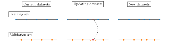
In classical training for machine learning models, we usually rely on a fixed amount of observations, which are splitted between training and validation sets (sometimes also on a test set). However, with the incresing machine learning models, different approaches to training were developed. Those techniques range from avoiding overfitting from large amount of data, to avoiding underfitting by generating new data from small training sets. The training time and final result of the training process will depend, among other elements, on the election of an adequate training set. Some well-known methodologies of adaptive training set are bootstrapping in neural networks [7], important sampling [21], and mesh refinement in PINNs [28]. We implement a methodology to add samples to training and validation sets at specific training epochs.

4.1 Adaptive generation of training data

We employ an adaptive training step to improve the training process without significantly increasing computational cost. Based on the idea of adaptive integration presented in [25], we define an adaptive training set that will iteratively incorporate the elements of the validation set with the worst performance (accordingly to certain criteria). Particularly in this work, we include in the training set those elements of the validation with a loss evaluation greater than $\gamma$ times the loss of the training set. Algorithm 1 describes this idea.

Algorithm 1 Adaptivity for the training set

$X_{\text{train}}$, $X_{\text{val}}$, $\gamma$

while stage $<$ $\#$stages do $\triangleright$ $\#$stages: number of stages to update the training set

     while epoch $<$ #epochs do $\triangleright$ $\#$epochs: number of epochs

         $\theta^{*}\leftarrow\operatorname*{argmin}_{\theta}\mathcal{L}(\theta;X_{\text{train}})$ $\triangleright$ neural network training

     end while

     $\mathcal{L}_{\text{train}}\leftarrow\mathcal{L}(\theta^{*};X_{\text{train}})$

     for $x_{\text{val}}\in X_{\text{val}}$ do

         if $\mathcal{L}(\theta^{*};\{x_{\text{val}}\})>\gamma\mathcal{L}_{\text{train}}$ then $\triangleright$ Chosen criteria

              $X_{\text{train}}\leftarrow X_{\text{train}}\cup\{x_{\text{val}}\}$

         end if

     end for

     update $X_{\text{val}}$ $\triangleright$ $X_{\text{val}}$ is updated when new points are added to $X_{\text{train}}$

end while

Remark 4.1.

If $\gamma$ is greater than one, we avoid overfitting by adding the validation-set points with a loss value that lags behind the training-set loss value.

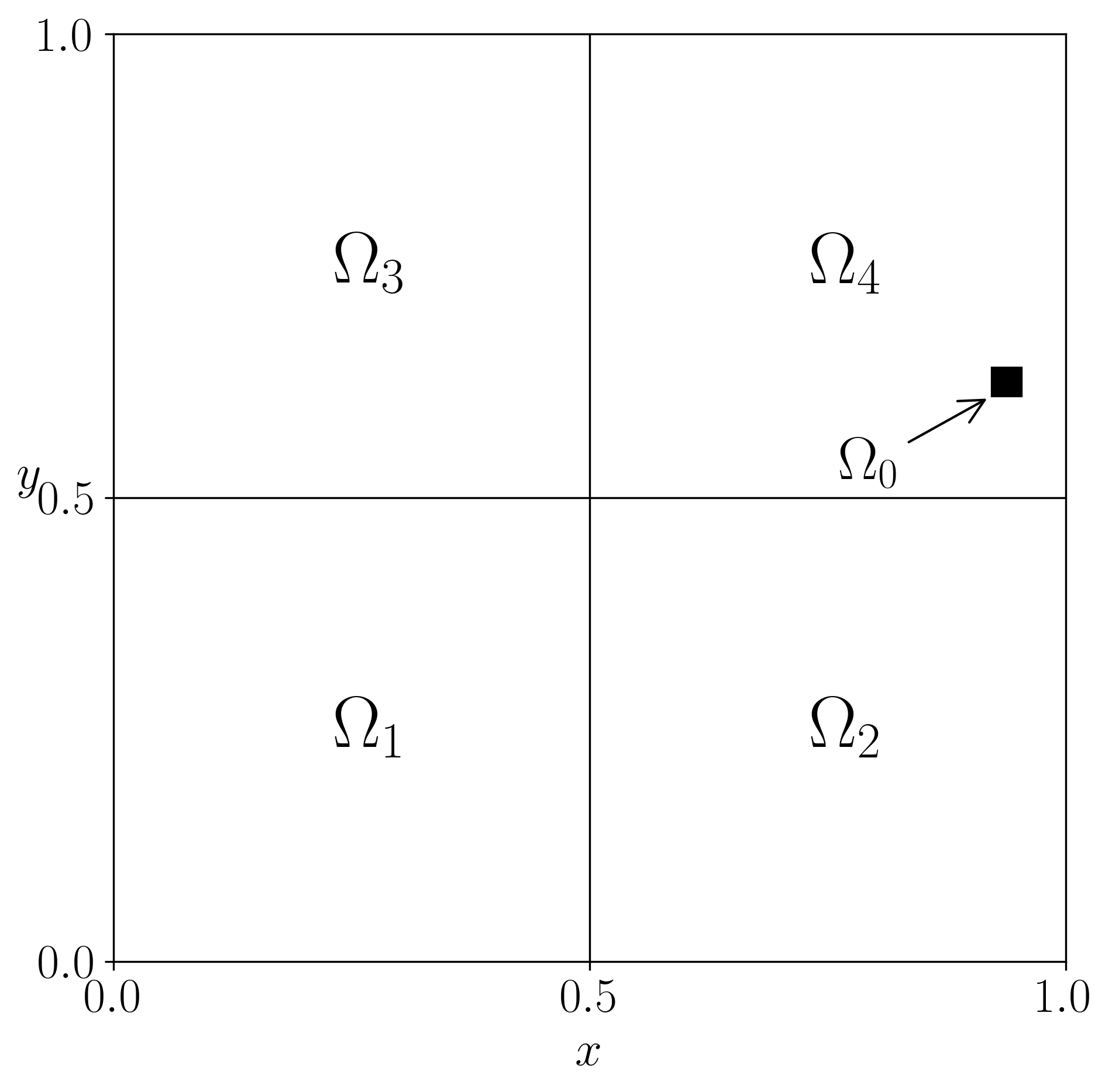
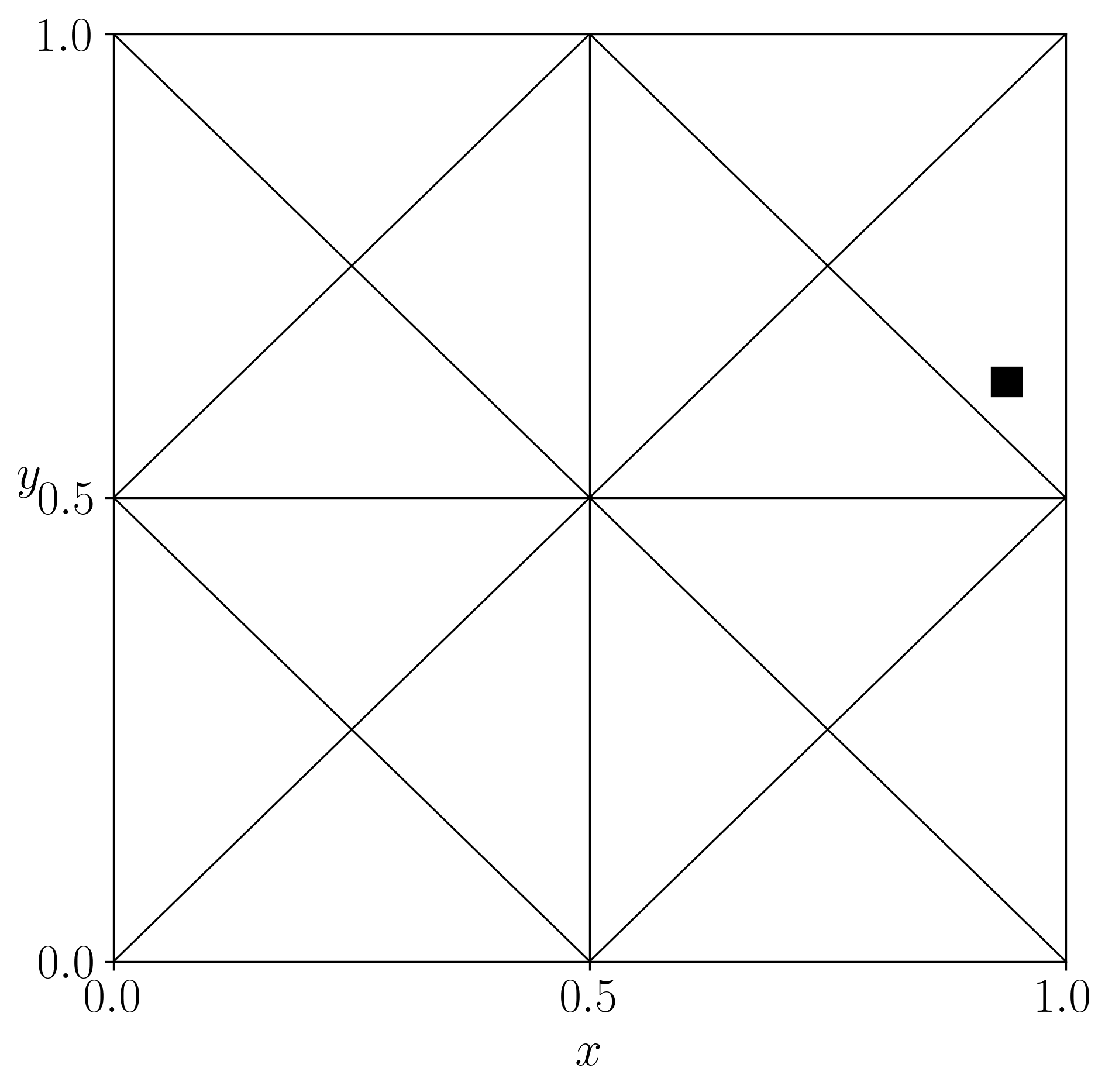
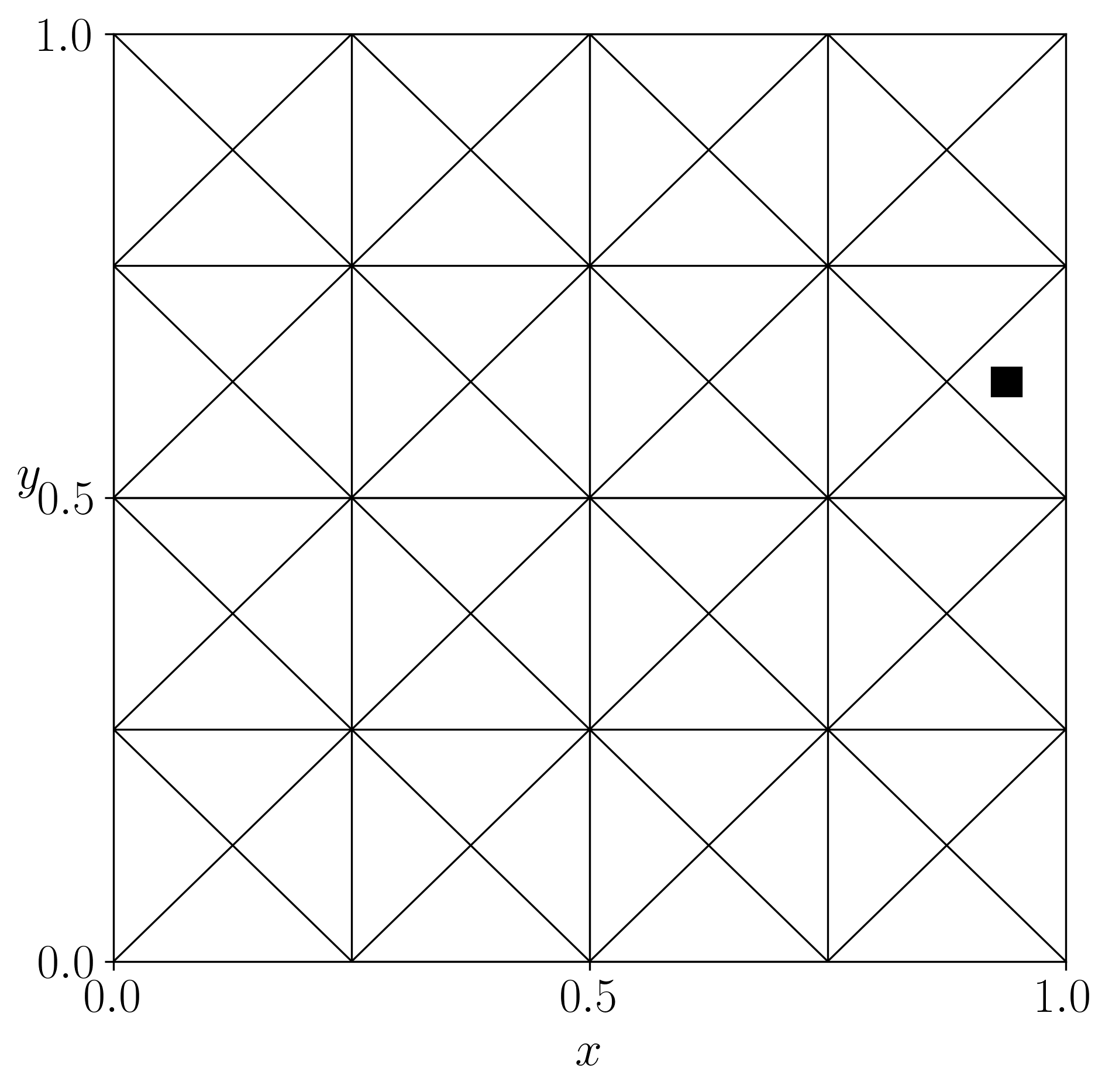
We propose as validation set the middle points (center of mass in higher dimensions) of the elements in the training. So each time that a validation-set point is included as part the training set, we update the validation set adding the new middle point from the training set. Figure 2 illustrate the procedure of training and validation set updates. For example,

1. Select a training set from coarse grid of the parameter space $\Lambda$.

2. We define the validation set as the middle points of the coarse grid.

3. Run a usual minimization method (SDG, Adam, RMSProp, etc) to train the artificial neural network with the above training set for a certain number of epochs.

4. Evaluate the loss function within the elements of the validation set.

5. Add the validation-set points with worst results to the training set (according to certain criteria, see Algorithm 1).

6. Update the validation set by removing the points added to the training set and adding the new needed middle points.

Figure 2: Adaptive training and validation sets.

5 Numerical Results

We present some numerical examples to show the different features of the method. In the next examples, unless otherwise stated, we employ feed-forward neural networks with three hidden layers and ten neurons on each hidden layer. The input of the neural network is the PDE parameter $\lambda$, then the input layer of the neural network has $\rho$ neurons (with $\rho:=\dim\Lambda$). The output of the neural network is the set of coefficients associated with the weighted inner product. Thus, for a piecewise constant weight function (i.e., $p=0$) defined on $n_{a}$ patches, the output layer contains $n_{a}$ neurons, i.e.,

$$\lambda\longrightarrow\text{NN}(\lambda;\theta)\longrightarrow\big{\{}c(\lambda,1;\theta),\dots,c(\lambda,n_{a};\theta)\big{\}}.$$

To ensure positive constants, we choose the $\operatorname{softplus}$ function as the activation function for the output layer (while the hyperbolic tangent function is used on every other layer). To train the neural network, we employ the Adam optimization algorithm [15] within TensorFlow, with decay rates $\beta_{1}=0.9$ and $\beta_{2}=0.999$, regularization term for numerical stability $\epsilon=1\text{e}^{-16}$, EMA momentum equal to $0.99$, and learning rate $\alpha=1.\text{e}^{-4}$. Table 1 displays a TensorFlow scheme of the neural network architecture.

ML-MinRes neural network architecture
Layer (type)	Output Shape	Activation Function
Input non-trainable layer ($\lambda$)	(None, $\rho$)	$\tanh$
Hidden Dense layer	(None, 10)	$\tanh$
Hidden Dense layer	(None, 10)	$\tanh$
Hidden Dense layer	(None, 10)	$\tanh$
Output Dense layer ($c$)	(None, $n_{a}$)	$\operatorname{softplus}$

Table 1: Neural network architecture employed in most of the following examples.

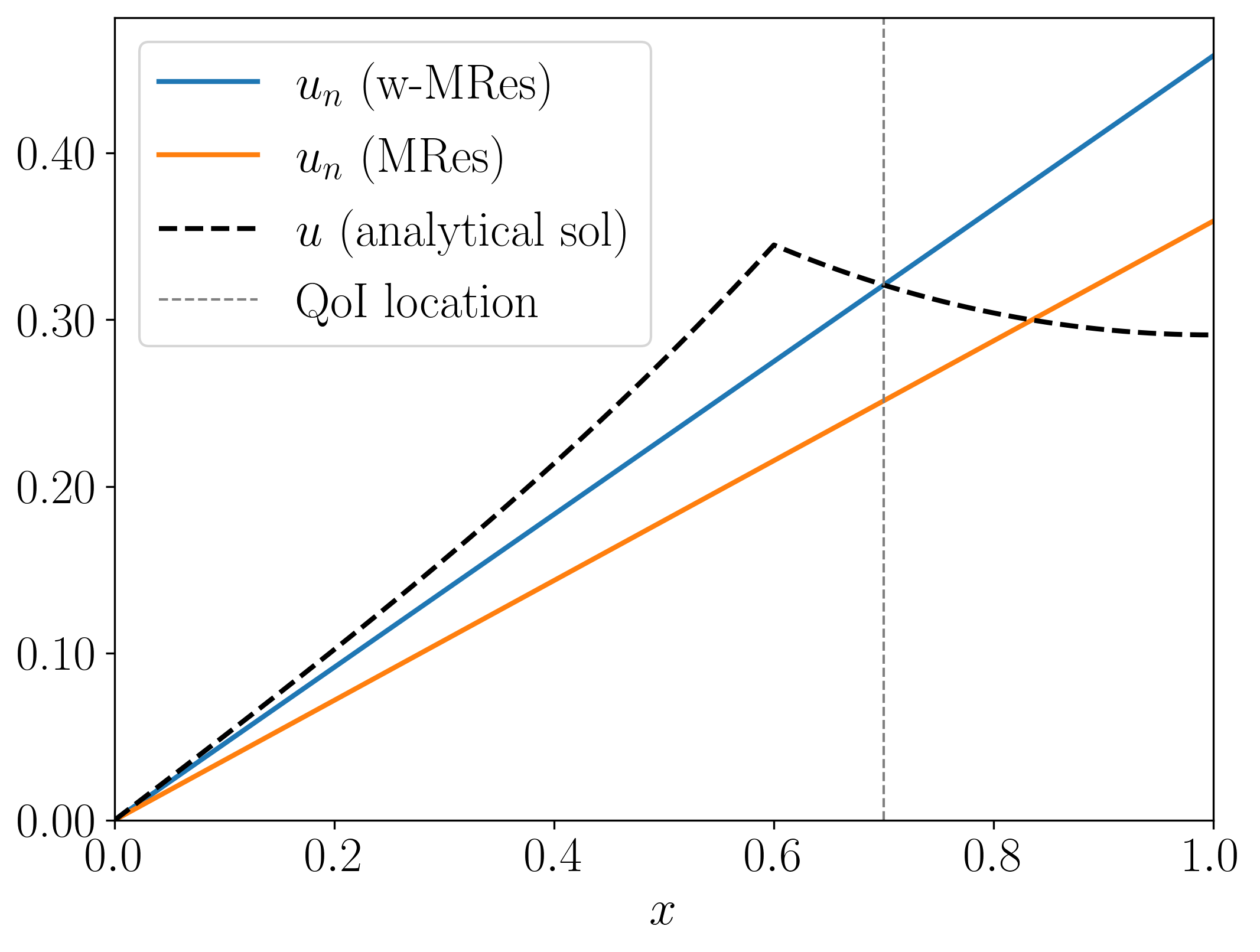
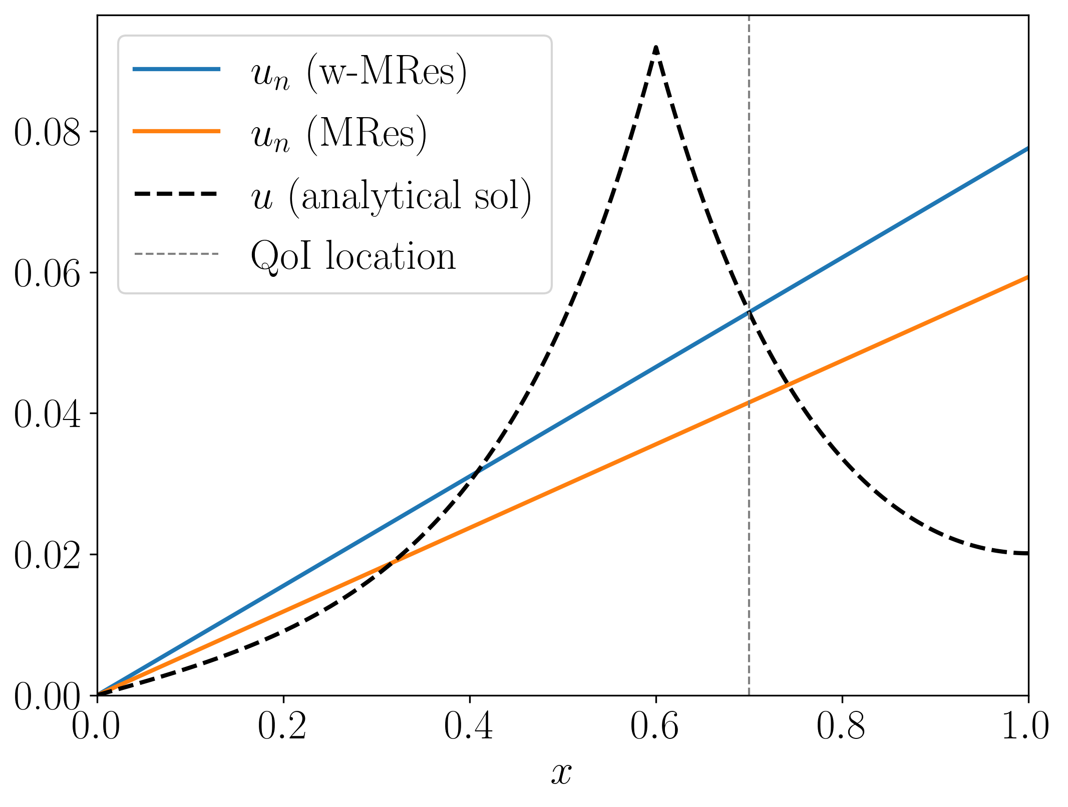
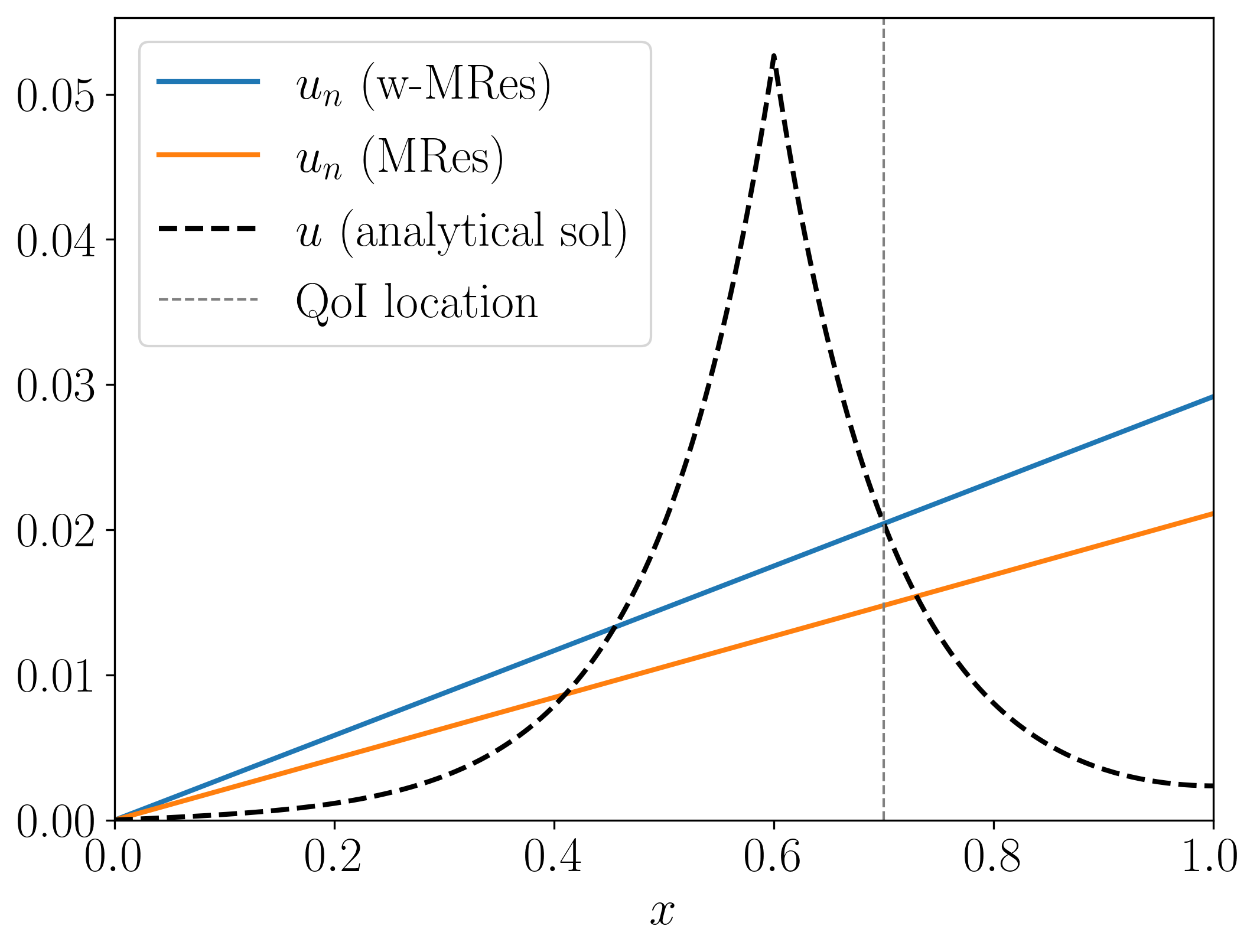
5.1 1D diffusion-reaction equation with one parameter

We consider a 1D diffusion-reaction equation with the parameter $\lambda$ in the reaction term. The right-hand side of this problem is given by a Dirac delta function located at $x_{0}=0.6$. Thus, we have the following problem:

$$\left\{\begin{array}[]{rll}-u_{xx}(x)+\lambda^{2}u(x)=&\delta_{x_{0}}(x)&\hbox{in }(0,1),\\ u(0)=&0,&\\ u^{\prime}(1)=&0,&\end{array}\right.$$ (13)

with $\lambda\in[1,10]$. We also define the linear quantity of interest $q:\mathbb{U}\to\mathbb{R}$ as

$$q(u)=u(0.7).$$

Notice that the exact solution to problem (13) is:

$$u_{\lambda}(x)=\begin{cases}c_{1}(\exp(\lambda x)-\exp(-\lambda x)),&\text{if }x<x_{0},\\ c_{2}\left(\exp(\lambda x)+\exp(\lambda(2-x))\right),&\text{if }x>x_{0},\end{cases}$$

where

$$c_{1}=\displaystyle\frac{1}{2\lambda}\frac{\exp(\lambda x_{0})+\exp(\lambda(2-x_{0}))}{1+\exp(2\lambda)}\qquad\hbox{ and }\qquad c_{2}=\displaystyle\frac{1}{2\lambda}\frac{\exp(\lambda x_{0})-\exp(-\lambda x_{0})}{1+\exp(2\lambda)}.$$

Given the continuous trial and test spaces $\mathbb{U}=\mathbb{V}=H_{(0}^{1}(0,1)$, we introduce the following variational formulation of problem (13):

$$\left\{\begin{array}[]{l@{\;}lr}\lx@intercol\text{Find }u\in\mathbb{U}\text{ such that:}\hfil\lx@intercol\\ \underbrace{\displaystyle\int_{0}^{1}u_{x}v_{x}}_{\left<B_{0}u,v\right>_{\mathbb{V}^{*},\mathbb{V}}}+\lambda^{2}\underbrace{\int_{0}^{1}uv}_{\left<B_{1}u,v\right>_{\mathbb{V}^{*},\mathbb{V}}}&=v(x_{0}),&\forall\,v\in\mathbb{V}.\end{array}\right.$$ (14)

Thus, we define $B_{\lambda}:\mathbb{U}\to\mathbb{V}^{*}$ as $B_{\lambda}:=B_{0}+\lambda^{2}B_{1}$ and $\ell_{\lambda}:=\delta_{x_{0}}$ (which is independent from $\lambda$).

In addition, we define the weighted inner product for the test space as

$$(r,v)_{\omega_{\mathrm{pw}}}:=\int_{0}^{1}\omega_{\mathrm{pw}}(x,\lambda)\big{(}r_{x}(x)v_{x}(x)+r(x)v(x)\big{)}\,dx,\quad\forall\,r,v\in\mathbb{V},$$ (15)

with the following piecewise constant inner-product weight:

$$\omega_{\mathrm{pw}}(x,\lambda):=\begin{cases}c(\lambda,1),&\text{if }x\in(0,1/4),\\ c(\lambda,2),&\text{if }x\in(1/4,1/2),\\ c(\lambda,3),&\text{if }x\in(1/2,3/4),\\ c(\lambda,4),&\text{if }x\in(3/4,0).\\ \end{cases}$$ (16)

The discrete trial space $\mathbb{U}^{n}$ will be the space generated by the function $\varphi(x)=x$, while the discrete test space $\mathbb{V}^{m}$ will consist of conforming piecewise linear functions over a uniform mesh of four elements. With all these ingredients we construct the mixed formulation (2) and proceed with the methodology described in Section 2. We use the neural network architecture described in Table 1 and no adaptive training has been performed for this case. The training set is composed of $N_{s}=10$ elements, such that $\lambda\in\{1,2,3,\dots,10\}$.

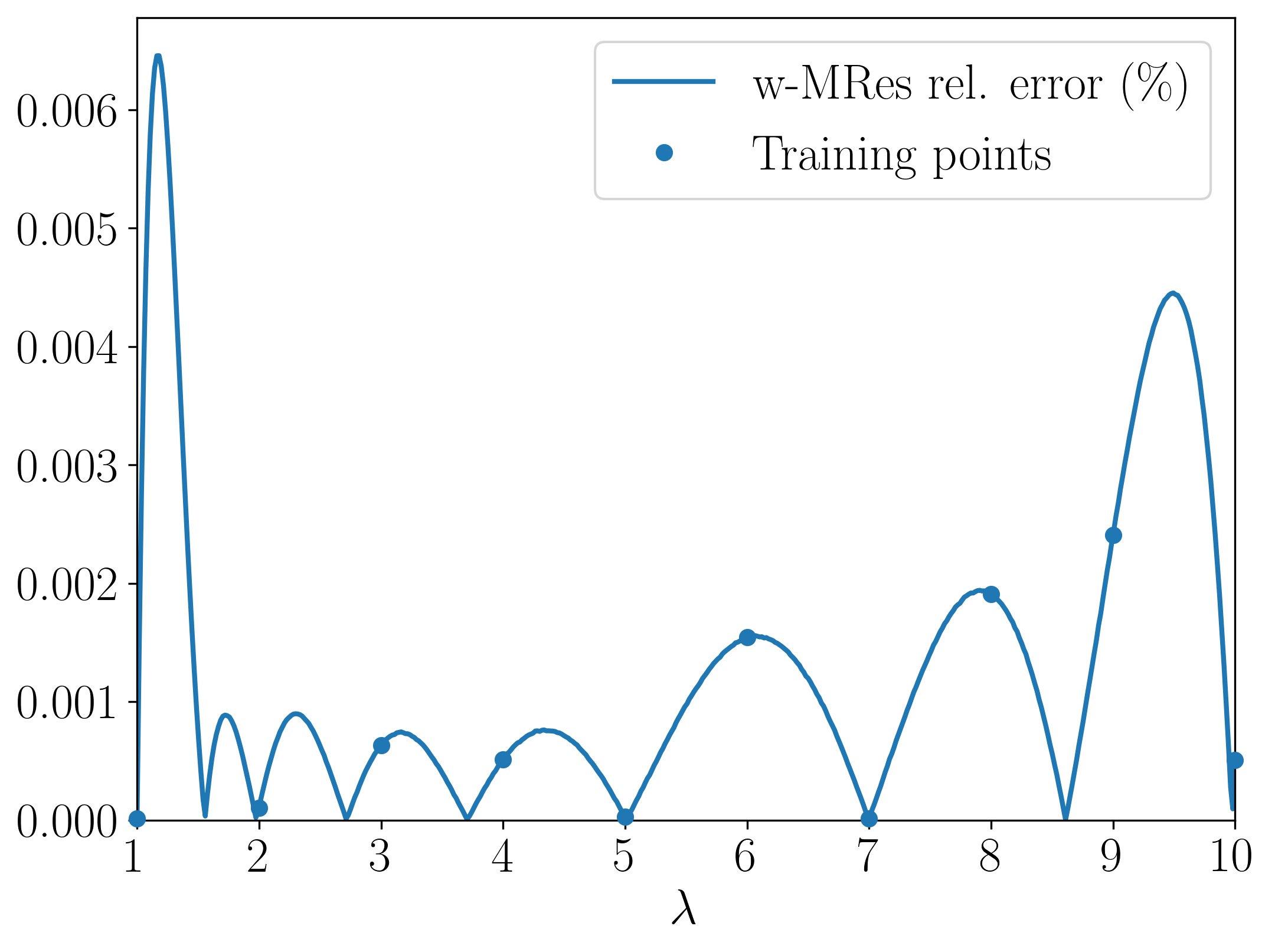
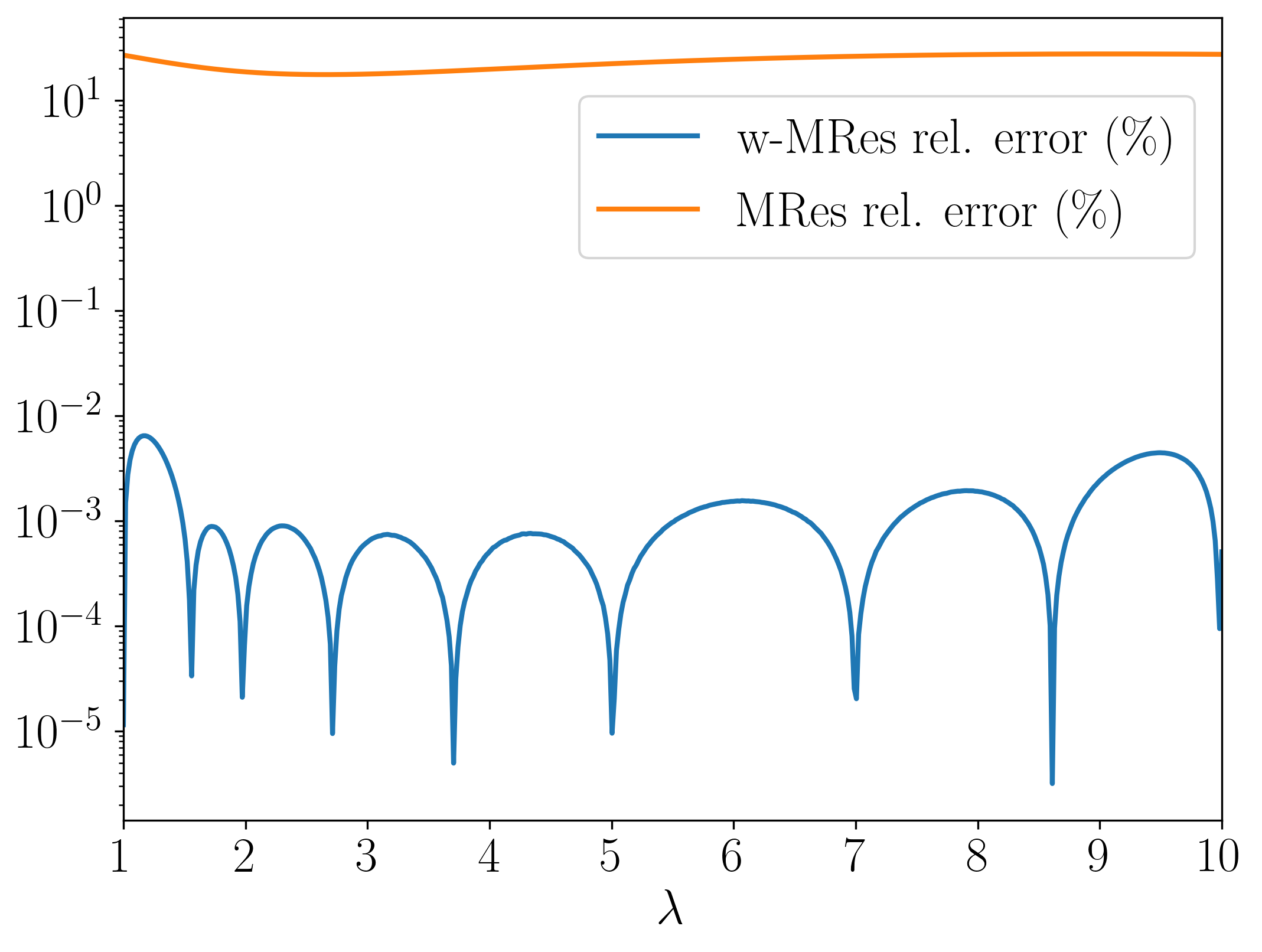
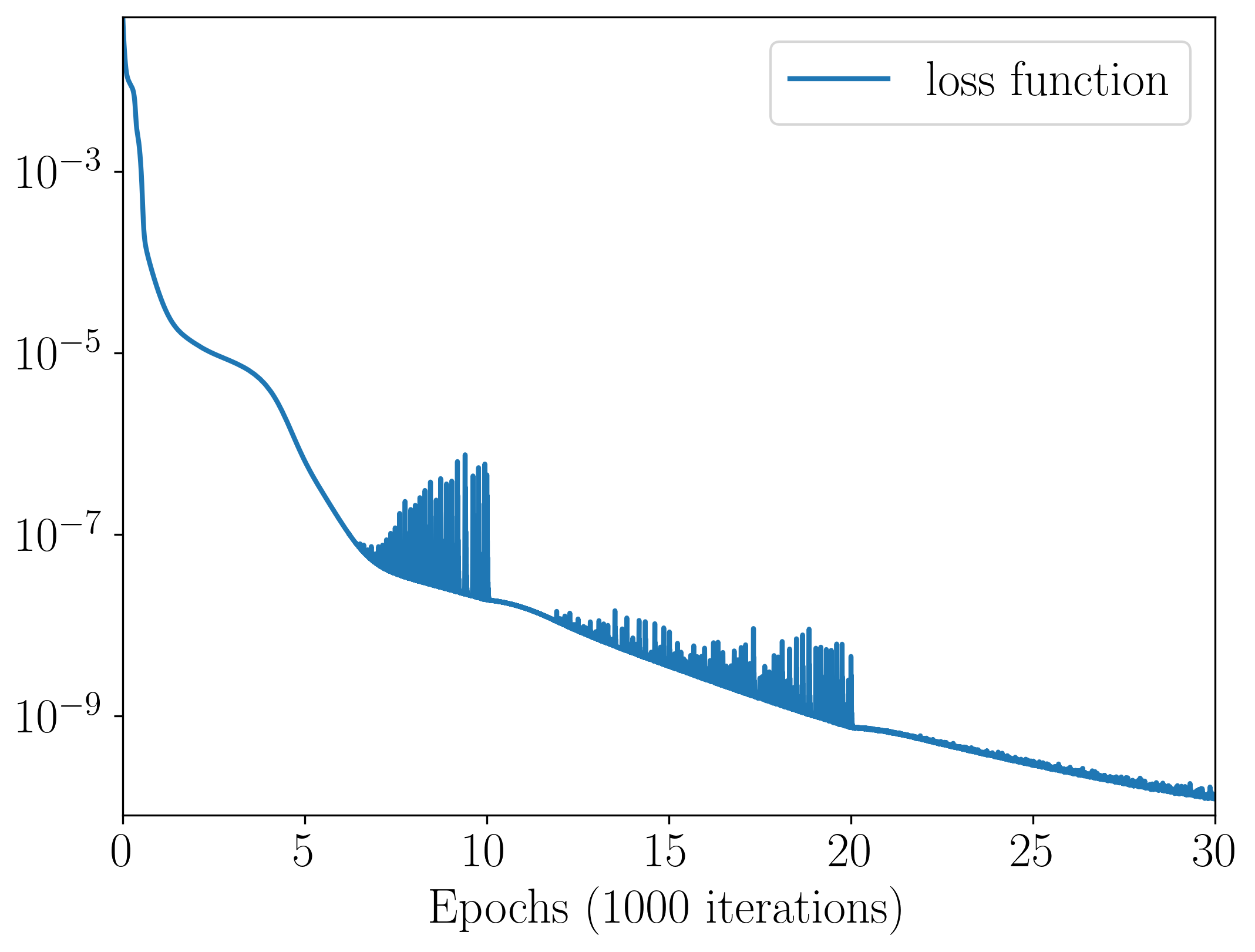
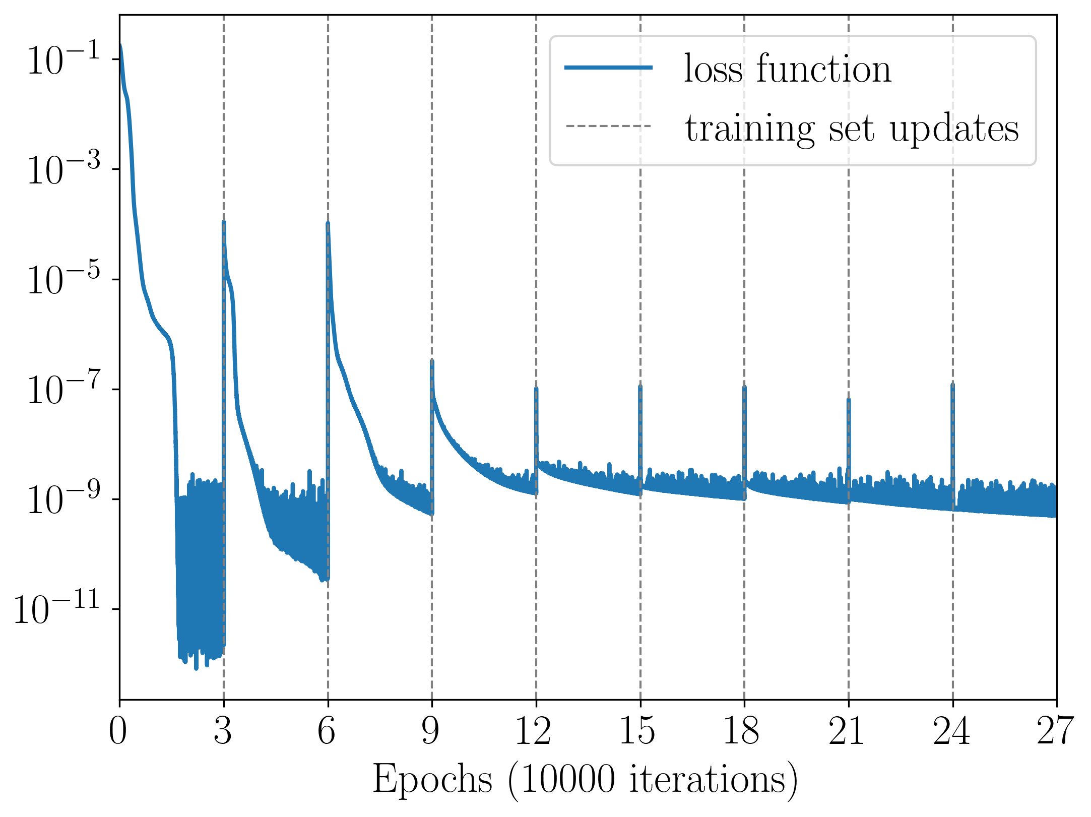
Figure 3 shows the performance of ML-MinRes or weighted-Minres (w-MinRes) method, after training the inner-product weight for the example described above. Subfigures 3(a), 3(b), and 3(c) show the results for the classical MinRes and the ML-MinRes methods for $\lambda\in\{1.5,5.5,9.5\}$. In blue, we observe the discrete solution computed from solving the system (2) with the optimal inner-product weight. In orange, we show the standard minimal residual scheme (with only one element). In black dashed line, we plot the exact solution to problem (13) as a reference. The grey dashed line shows the quantity of interest location. Subfigure 3(d) shows the relative error in linear scale for a fine-grid test set (grid for $\Lambda$) and also display the training points. Subfigure 3(e) compares the relative error in logarithmic scale between the MinRes and ML-MinRes methods for a fine-grid test set. The last subfigure shows the loss function through epochs. Notice that for this training we employed three different learning rates $[1\text{e}^{-3},1\text{e}^{-4},1\text{e}^{-5}]$, each one for $10.000$ iterations, in order to avoid oscillations in the loss function.

(a) results for $\lambda=1.5$

(b) results for $\lambda=5.5$

(c) results for $\lambda=9.5$

(d) w-MinRes method rel. error

(e) comparison rel. error (log scale)

(f) loss function

Figure 3: ML-MinRes performance for 1D parametric diffusion reaction example.

5.2 1D diffusion-reaction equation with two parameters

We consider 1D diffusion-reaction problem with a two-dimensional parameter $\lambda=(\alpha,\beta)$. The right-hand side of this problem is given by a Dirac delta function located at $x_{0}=0.6$. The first component of the parameter $\alpha$ multiplies the diffusion term and the second component $\beta$ multiplies the reaction term. Thus, we have the following problem:

$$\left\{\begin{array}[]{rll}-\alpha^{2}u_{xx}(x)+\beta^{2}u(x)&=\delta_{x_{0}}(x),&\hbox{in }(0,1).\\ u(0)&=0,&\\ u^{\prime}(1)&=0,&\end{array}\right.$$ (17)

with $\lambda=(\alpha,\beta)\in[1,10]^{2}$. We set the quantity of interest as $q(u)=u(0.7)$. Notice that the exact solution to this problem (17) is

$$u_{\lambda}(x)=\begin{cases}\displaystyle c_{1}\left(\exp\left(\frac{\beta}{\alpha}x\right)-\exp\left(-\frac{\beta}{\alpha}x\right)\right),&\text{if }x<x_{0},\\ \displaystyle c_{2}\left(\exp\left(\frac{\beta}{\alpha}x\right)+\exp\left(\frac{\beta}{\alpha}(2-x)\right)\right),&\text{if }x>x_{0},\end{cases}$$ (18)

where

$$c_{1}=\frac{1}{2\alpha\beta}\frac{\displaystyle\exp\left(\frac{\beta}{\alpha}x_{0}\right)+\exp\left(\frac{\beta}{\alpha}(2-x_{0})\right)}{\displaystyle 1+\exp\left(2\frac{\beta}{\alpha}\right)}\quad\text{ and }\quad c_{2}=\frac{1}{2\alpha\beta}\frac{\displaystyle\exp\left(\frac{\beta}{\alpha}x_{0}\right)-\exp\left(-\frac{\beta}{\alpha}x_{0}\right)}{\displaystyle 1+\exp\left(2\frac{\beta}{\alpha}\right)}.$$

As in the previous example, we set the trial and test spaces to be $\mathbb{U}=\mathbb{V}=H_{(0}^{1}(0,1)$, and the variational formulation is given by

$$\left\{\begin{array}[]{l@{\;}lr}\lx@intercol\text{Find }u\in\mathbb{U}\text{ such that:}\hfil\lx@intercol\\ \displaystyle\alpha^{2}\underbrace{\int_{0}^{1}u_{x}v_{x}}_{\left<B_{1}u,v\right>_{\mathbb{V}^{*},\mathbb{V}}}+\beta^{2}\underbrace{\int_{0}^{1}uv}_{\left<B_{2}u,v\right>_{\mathbb{V}^{*},\mathbb{V}}}&=\displaystyle v(x_{0}),&\forall\,v\in\mathbb{V}.\end{array}\right.$$ (19)

Thus, we define $B_{\lambda}:\mathbb{U}\to\mathbb{V}^{*}$ as $B_{\lambda}:=\alpha^{2}B_{1}+\beta^{2}B_{2}$ and $\ell_{\lambda}:=\delta_{x_{0}}$ (which is independent from $\lambda$). In addition, we use the same inner product defined in (15)-(16), together with the same (discrete) trial and test space of the previous example in Section 5.1.

Notice that in this example, the artificial neural network has two neurons in the input layer (and four in the output layer). For the training set, we select 100 equispaced elements in the set $(1,10)\times(1,10)$ (see red dots in Subfigure 4(b)). In addition, we employed three different learning rates $[1\text{e}^{-3},1\text{e}^{-4},1\text{e}^{-5}]$ during the training, each one for $15.000$ iterations.

(a) loss function

(b) w-MinRes method rel. error

Figure 4: ML-MinRes performance for two-parameters diffusion reaction example. Red dots show the training points.

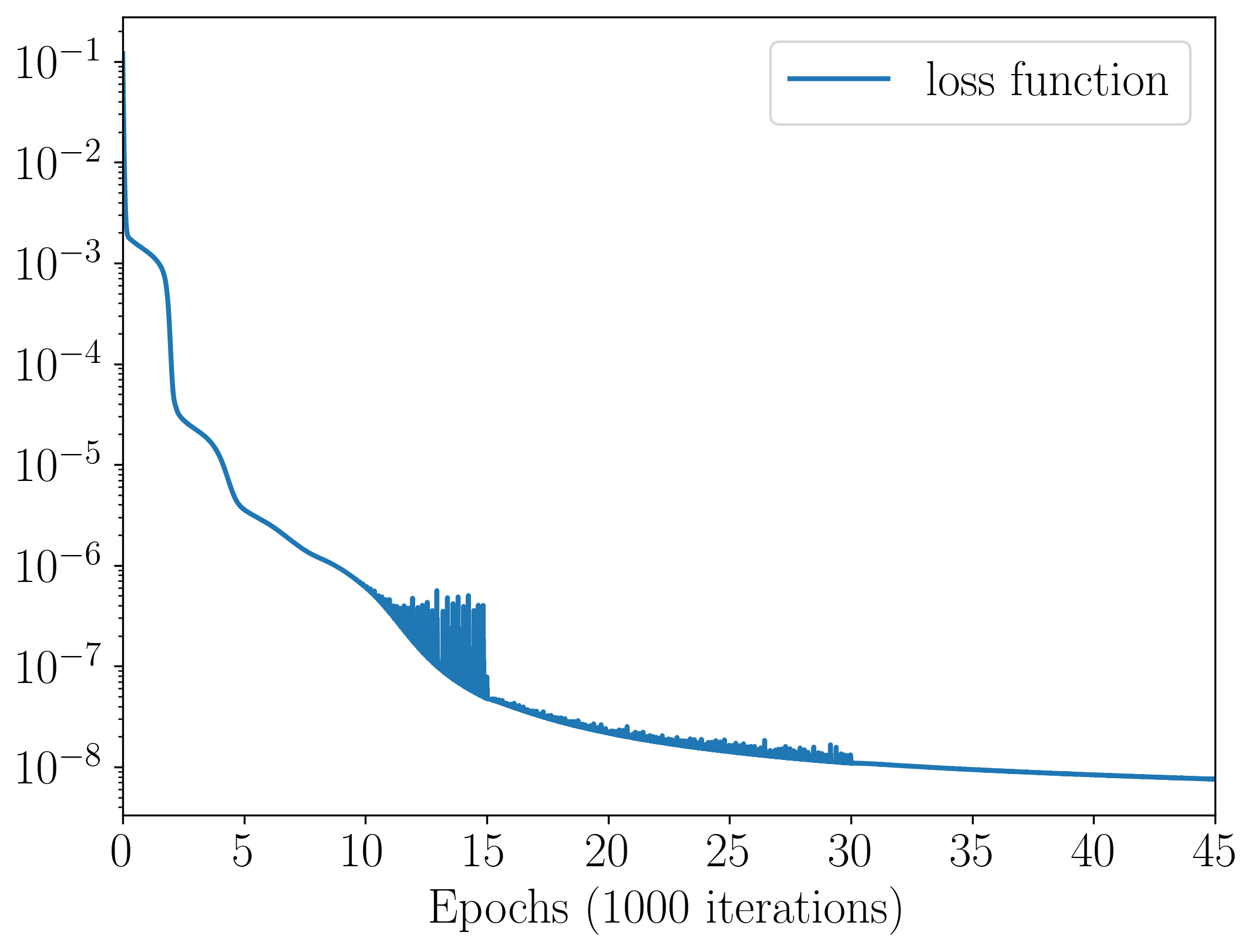
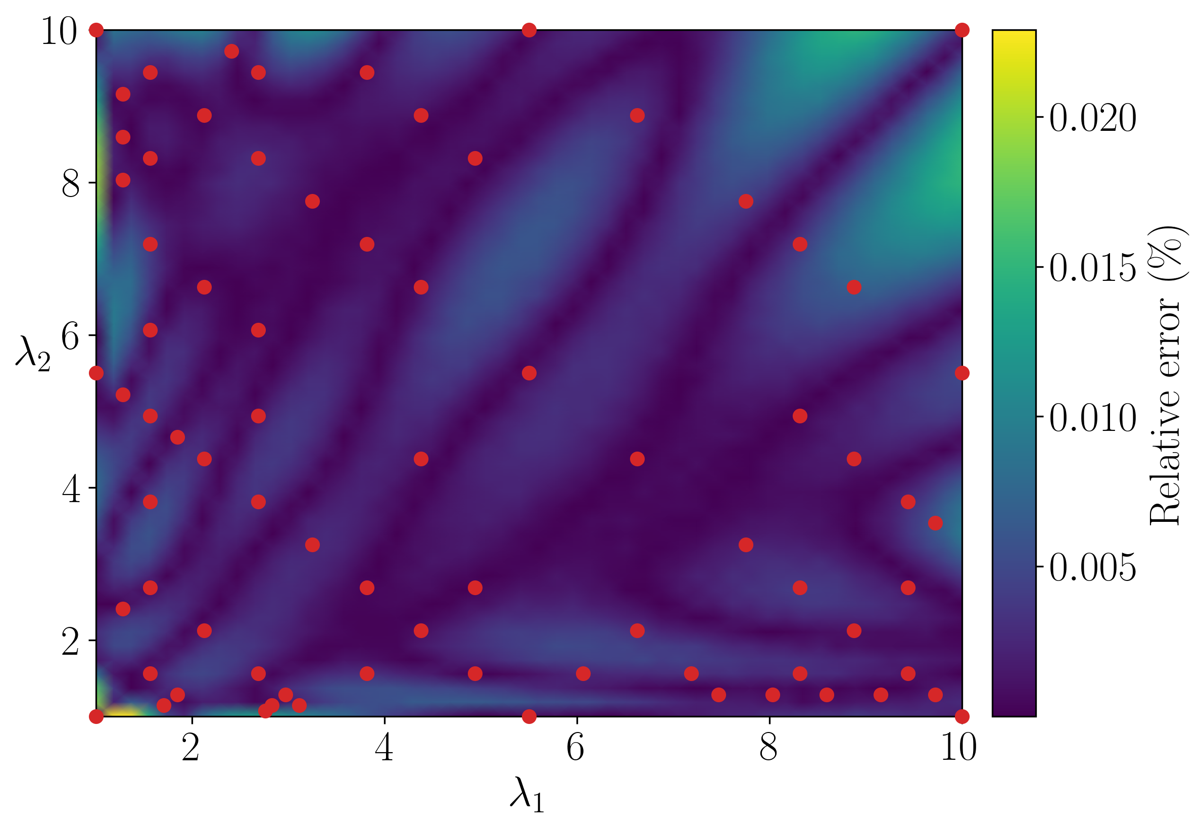
Subfigure 4(a) displays the loss function through epochs for the three different learning rates $[1\text{e}^{-3},1\text{e}^{-4},1\text{e}^{-5}]$. Subfigure 4(b) shows the relative error in linear scale for a test set (fine-grid in $\Lambda$) and also display the training points in red dots. The picture shows that the relative error is below $0.5\%$ after the training.

5.3 1D advection with parametric right-hand side

Let us consider the parametric 1D advection problem:

$$\left\{\begin{array}[]{rll}u_{x}(x)&=f_{\lambda}(x),&\hbox{in }(0,1),\\ u(0)&=0,&\end{array}\right.$$ (20)

where $f_{\lambda}(x):=(x-\lambda)(x>\lambda)$, with $\lambda\in\Lambda:=[0,1]$. We set the quantity of interest as $q(u)=u(0.9)$.

Notice that the exact solution to this problem is

$$u(x)=\left\{\begin{array}[]{rc}(x-\lambda)^{2},&\textrm{ if }x>\lambda,\\ 0,&\textrm{ if }x<\lambda.\end{array}\right.$$

We define the variational formulation,

$$\left\{\begin{array}[]{lr}\text{Find }u\in H_{(0}^{1}(0,1)\text{ such that}\\ \underbrace{\displaystyle\int_{0}^{1}u_{x}v}_{\left<Bu,v\right>_{\mathbb{V}^{*},\mathbb{V}}}=\underbrace{\int_{0}^{1}f_{\lambda}v}_{\left<\ell_{\lambda},v\right>_{\mathbb{V}^{*},\mathbb{V}}},&\forall\,v\in L^{2}(0,1),\end{array}\right.$$ (21)

Notice that here $\mathbb{U}=H_{(0}^{1}(0,1)$ and $\mathbb{V}=L^{2}(0,1)$. In addition, we use the same inner product defined in (15)-(16), together with the same (discrete) trial space of the previous example in Section 5.1. However, the discrete test space is a piecewise constant space over four uniform elements (same as the weight).

For this example, we employ the adaptive training set strategy from Subsection 4.1, with $30000$ epoch per stage and $\gamma=5$. We also define the initial training set $\{(\lambda_{i},q_{\lambda_{i}})\}_{i=1}^{N_{s}}$ composed of $N_{s}=11$ elements such that $\lambda_{i+1}-\lambda_{i}=0.1$ for all $i\in\{1,2,\dots,N_{s}-1\}$. Notice that some quantities of interest may be zero, so in this case we modify the loss function, by adding a small regularization term

$$\mathcal{L}_{\mathrm{reg}}\left(\theta;\{\lambda_{i},q_{\lambda_{i}}\}_{i=1}^{N_{s}}\right):=\frac{1}{N_{s}}\sum_{i=1}^{N_{s}}\frac{1}{2}\left|\frac{q_{\lambda_{i}}-q(u_{n,\lambda_{i}}(\theta))}{q_{\lambda_{i}}+\epsilon_{0}}\right|^{2},$$

where $\epsilon_{0}=10^{-6}$.

(a) w-MinRes rel. error (fixed train.)

(b) comparison rel. error (fixed train.)

(c) loss function (fixed train.)

(d) w-MinRes rel. error (adapt. train.)

(e) comparison rel. error (adaptive train.)

(f) loss function (adaptive train.)

Figure 5: ML-MinRes performance for a 1D advection example with parametric right-hand side. First row shows the results for a fixed training set. The second row displays the results for an adaptive strategy.

(a) adaptive training-points generation

(b) comparison with unif. refinement

Figure 6: ML-MinRes Adaptive selection of training set and a comparison with uniform refinement for a 1D advection example with parametric right-hand side.

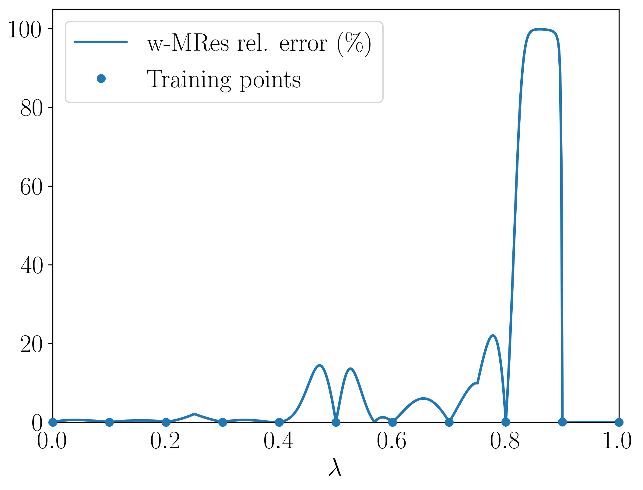
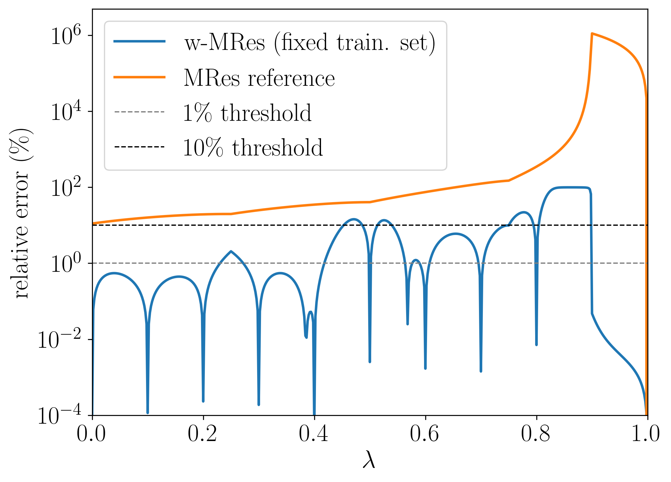
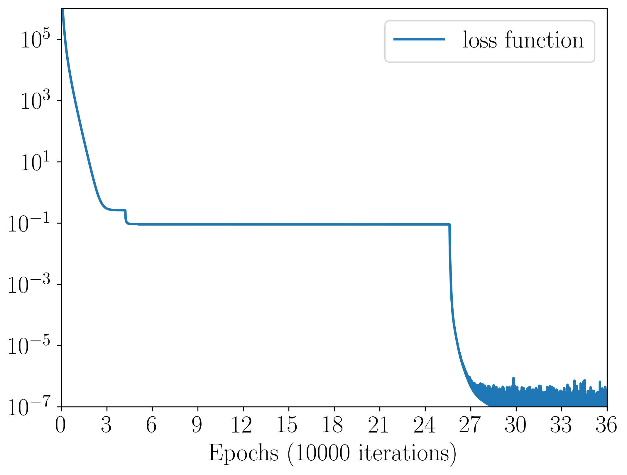
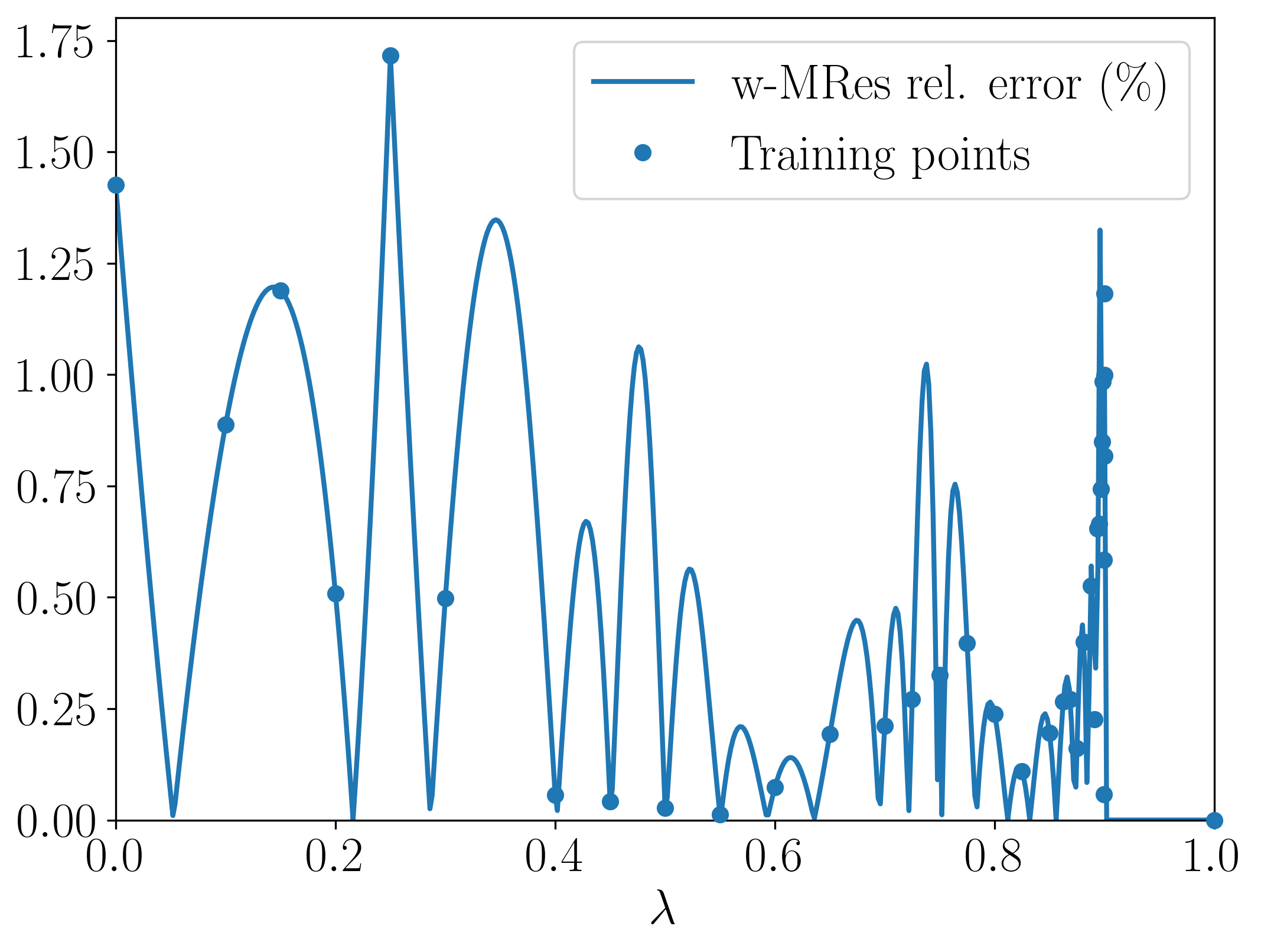
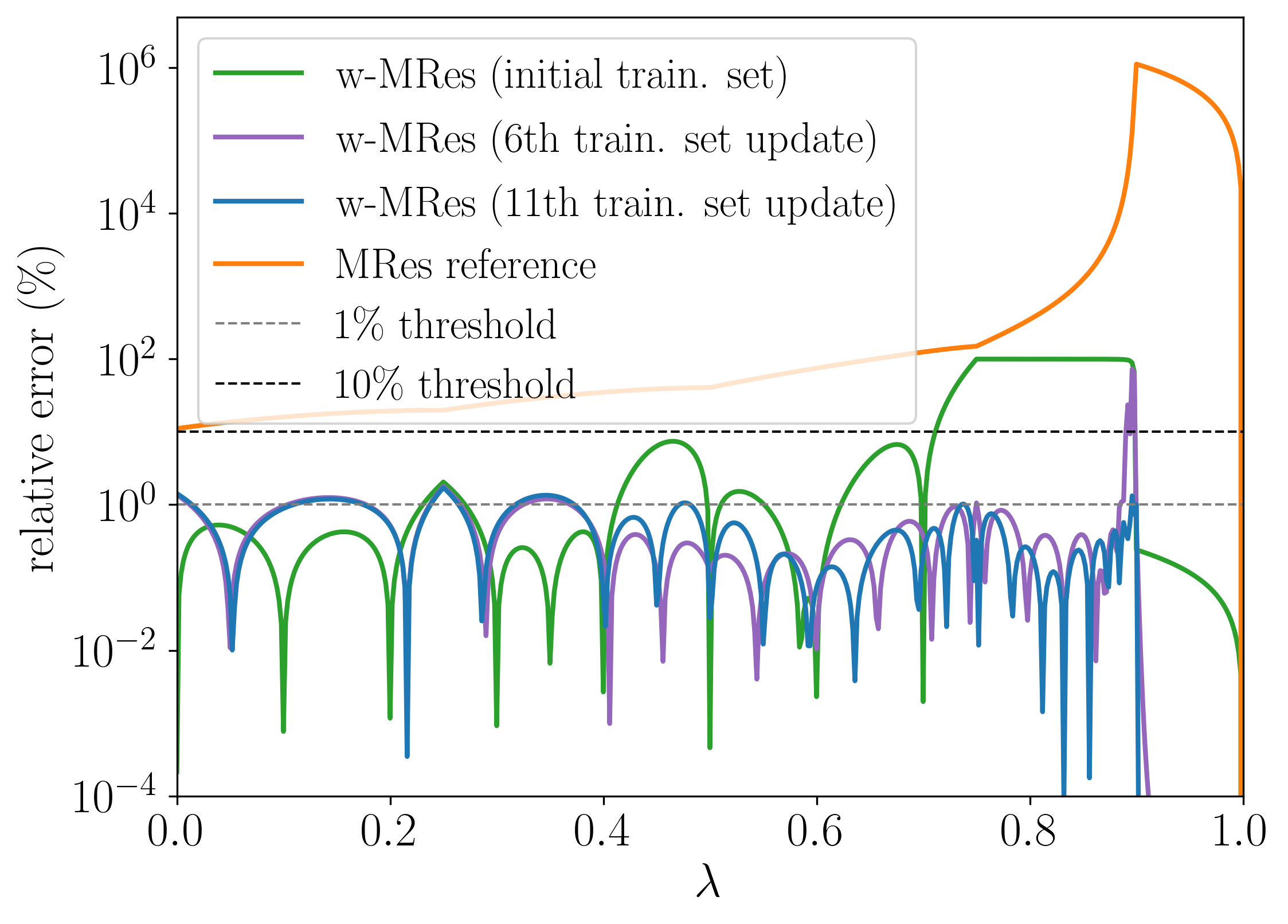
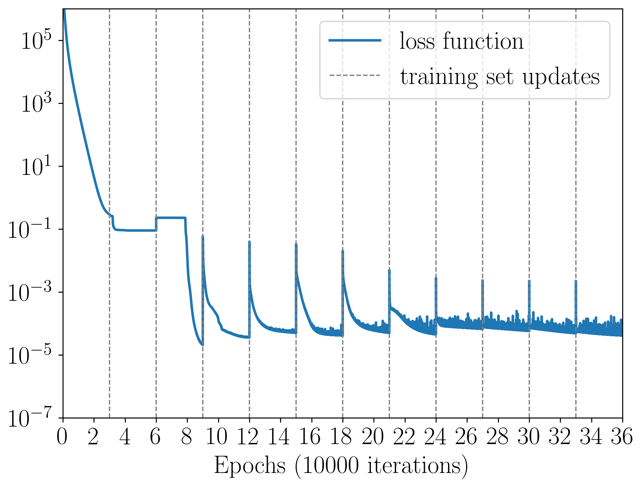
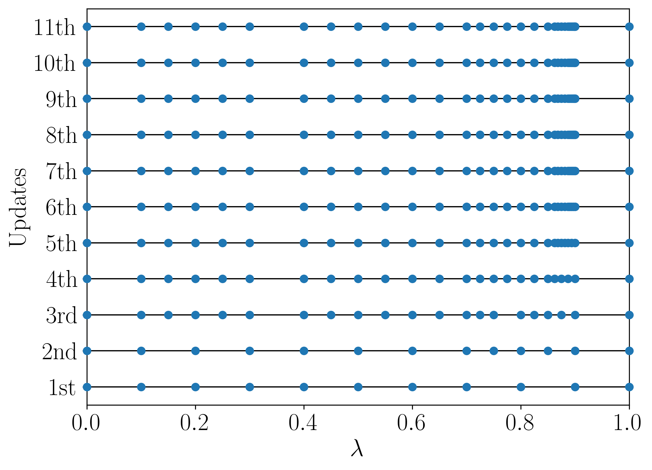
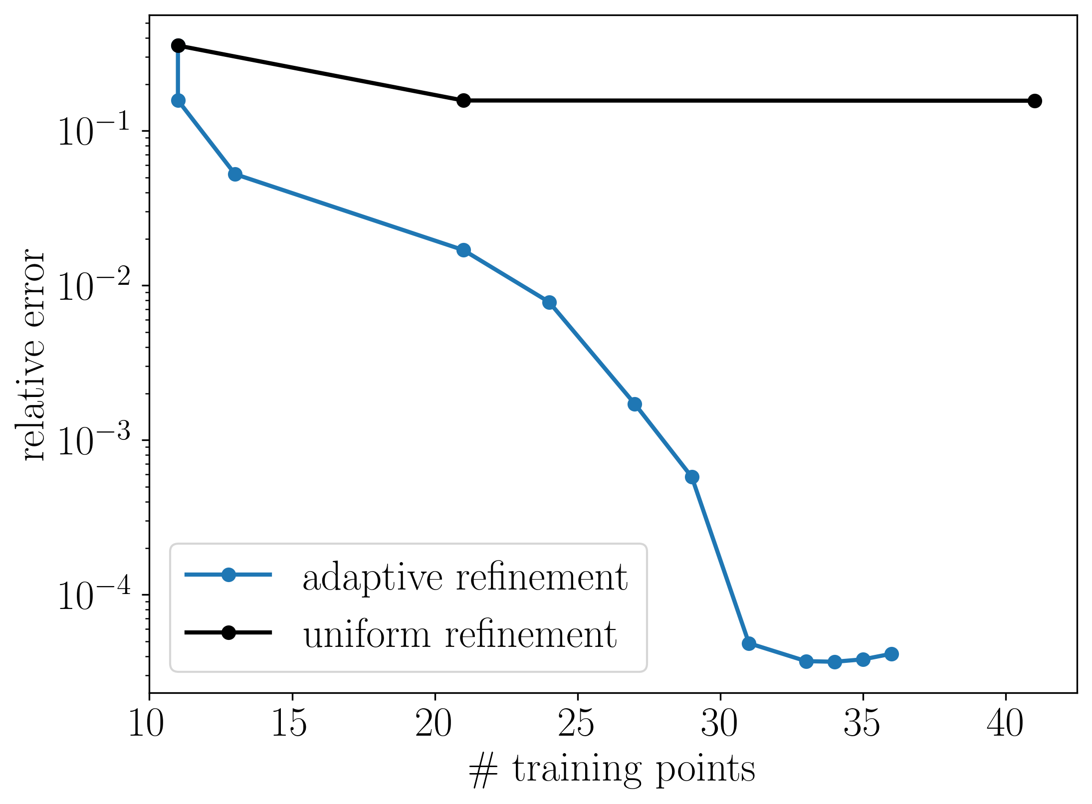
Figure 5 shows the results for the ML-MinRes with a fixed trained set (first row) and with the adaptive training set strategy (second and third rows) presented in Subsection 4.1. Subfigures in the first column show the the relative error in linear scale for the training with a fixed training set (Subfigure 5(a)) and the adaptive training set (Subfigure 5(d)). Subfigures 5(b) and 5(e) compare the relative error in logarithmic scale between MinRes and ML-MinRes with fixed and adaptive training set. The last column displays the loss function for both cases. Notice that in this example, the fixed training set with eleven elements poorly captures the quantity of interest behavior. This is because the training set does not represent the map between $\lambda$ and the quantity of interest. Then, the relative error increases drastically between 0.8 and 0.9 (see Subfigure 5(a)), even when the loss function is small. Then, the adaptive training set emerges as a good alternative to overcome the problem in this type of scenarios.

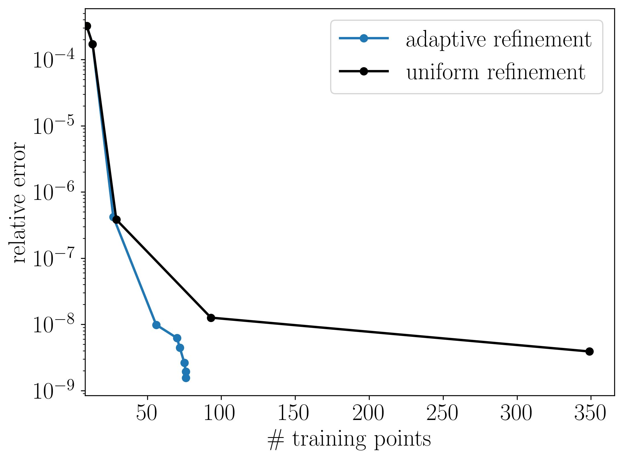
Finally, the Figure 6 shows the adaptive training-points generation, and a comparison with uniform refinement. In Subfigure 6(b) we can see the behaviour of the relative error for a test set (different form the adaptive training set) when we add points to the training set with adaptive (blue line) and uniform (black line) refinements after $30000$ epoch per refinement.

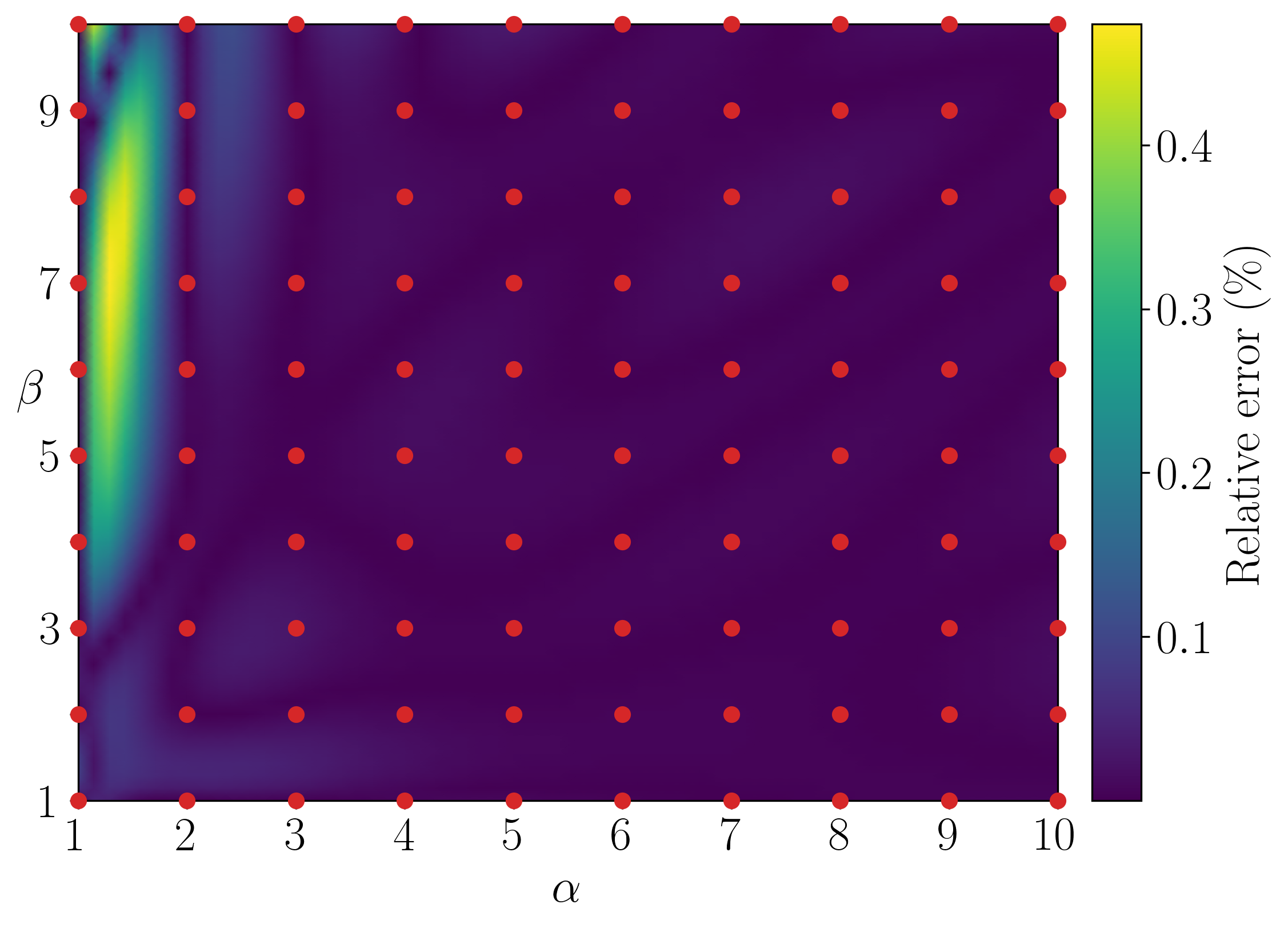
5.4 2D discontinuous-media diffusion equation with two parameters

Now, we consider a 2D diffusion equation, where the thermal conductivity is given by a two-dimensional parameter $\lambda=(\lambda_{1},\lambda_{2})$. Thus, we have the following problem:

$$\left\{\begin{array}[]{rl}-\nabla\cdot(a(x,y)\nabla u)=1,&\hbox{in }\Omega:=(0,1)^{2},\\ u=0,&\hbox{on }\partial\Omega,\end{array}\right.$$ (22)

where

$$a(x,y)=\begin{cases}\lambda_{1},&\text{if }(x,y)\in\Omega_{1}\cup\Omega_{3},\\ \lambda_{2},&\text{if }(x,y)\in\Omega_{2}\cup\Omega_{4},\end{cases}$$

with $\Omega_{1}=(0\,,0.5)^{2}$, $\Omega_{2}=(0.5\,,1)\times(0\,,0.5)$, $\Omega_{3}=(0\,,0.5)\times(0.5\,,1)$, and $\Omega_{4}=(0.5\,,1)^{2}$. See Subfigure 7(a).

(a) domain subdivision on $\Omega$

(b) trial-space mesh

(c) test-space mesh

Figure 7: Domain subdivision and meshes for discretization. Back square represents the QoI location.

Here, the quantity of interest is given by

$$q(u)=\frac{1}{\Omega_{0}}\int_{\Omega_{0}}u\,,$$

where, $\Omega_{0}=(0.9375-\frac{1}{2^{6}}\,,0.9375+\frac{1}{2^{6}})\times(0.625-\frac{1}{2^{6}}\,0.625+\frac{1}{2^{6}})$.

Given the continuous trial and test spaces $\mathbb{U}=\mathbb{V}=H_{0}^{1}(\Omega)$, we can obtain the following variational formulation:

$$\left\{\begin{array}[]{l@{\;}lr}\lx@intercol\text{Find }u\in\mathbb{U}\text{ such that:}\hfil\lx@intercol\\ \lambda_{1}\underbrace{\displaystyle\int_{\Omega_{1}\cup\Omega_{3}}\nabla u\cdot\nabla v}_{\left<B_{1}u,v\right>_{\mathbb{V}^{*},\mathbb{V}}}+\lambda_{2}\underbrace{\int_{\Omega_{2}\cup\Omega_{4}}\nabla u\cdot\nabla v}_{\left<B_{2}u,v\right>_{\mathbb{V}^{*},\mathbb{V}}}&=\underbrace{\displaystyle\int_{\Omega}v}_{\left<\ell,v\right>_{\mathbb{V}^{*},\mathbb{V}}},&\forall\,v\in\mathbb{V}.\end{array}\right.$$ (23)

Thus, we define $B_{\lambda}:\mathbb{U}\to\mathbb{V}^{*}$ as $B_{\lambda}:=\lambda_{1}B_{1}+\lambda_{2}B_{2}$. Additionally, we define the following weighted inner product:

$$(r,v)_{\omega_{\text{pw}}}:=\int_{\Omega}\omega_{\text{pw}}\nabla r\cdot\nabla v\,,\quad\forall\,r,v\in\mathbb{V},$$

where $\omega_{\text{pw}}$ is a constant value on each element of the test-space mesh (64 constants, see Figure 7(c)).

The discrete trial space $\mathbb{U}_{n}$ is given by piecewise linear functions with $n=5$ on a coarse mesh (see Figure 7(b)), while the discrete test space $\mathbb{V}_{m}$ is given by piecewise linear functions with $m=25$ on the mesh depicted in Figure 7(c).

(a) loss function

(b) w-MinRes method rel. error

(c) refinement comparison

Figure 8: ML-MinRes performance for two-parameters diffusion reaction example. Red dots show the training points.

On this example, we employ the adaptive adaptive training set with eight stages, $30000$ epoch per stage and $\gamma=5$. We also define the initial training set composed of $N_{s}=9$ elements, composed by $\{1,5.5,10\}\times\{1,5.5,10\}$ (Cartesian product).

Figure 8 displays the results for the ML-MinRes after training with an adaptive training-set strategy. Subfigure 8(a) displays the loss function through the six stages of the adaptive training. Subfigure 8(b) shows the the relative error (%) in linear scale for full test set after the training with an adaptive training set. Red dot represent the final training set. In Subfigure 8(c) we can compare the behaviour of the relative error of a test set when we add points to the training set with adaptive (blue line) and uniform (black line) refinements after $30000$ epoch per refinement.

6 Conclusions

In the present work, the extend the Machine Learning Minimal-Residual (ML-MinRes) method [2] and [3] to a more general framework of parametric PDEs. The main idea is to compute some high-precision quantity of interest of the solution using finite-element coarse meshes. This finite element scheme will generate a cheap and accurate method for the quantity of interest. As part of the main new features, we highlight the following:

• We avoid the problem of integrating a neural network by replacing the inner-product weight with a piecewise-polynomial weight (with coefficients delivered by a neural network). In this way, we have exact integration with quadrature rules.

• The piecewise polynomial weight for the inner product and the affine decomposition for $B_{\lambda}$ and $\ell_{\lambda}$ allow to pre-assemble the matrices. This fact helps to perform more efficient training and faster online evaluation after training.

• We propose an adaptive training set that allows for faster and more accurate neural network training. From the numerical experiments, we can see that adaptive training performs better than uniform refinements. In addition, it helps to reduce overfitting.

References

- [1] K. Bhattacharya, B. Hosseini, N. B. Kovachki, and A. M. Stuart, Model reduction and neural networks for parametric PDEs, The SMAI journal of computational mathematics, 7 (2021), pp. 121–157.
- [2] I. Brevis, I. Muga, and K. G. van der Zee, A machine-learning minimal-residual (ML-MRes) framework for goal-oriented finite element discretizations, Comput. Math. Appl., 95 (2021), pp. 186–199. Recent Advances in Least-Squares and Discontinuous Petrov–Galerkin Finite Element Methods.
- [3] I. Brevis, I. Muga, and K. G. van der Zee, Neural control of discrete weak formulations: Galerkin, least-squares and minimal-residual methods with quasi-optimal weights, Comput. Methods Appl. Mech. Engrg., 402 (2022), p. 115716.
- [4] A. Cohen, W. Dahmen, and R. DeVore, State estimation – the role of reduced models, in Recent Advances in Industrial and Applied Mathematics, ICIAM 2019, T. C. R. et al., ed., SEMA SIMAI Springer Series 1, Springer, 2022, pp. 57–77.
- [5] L. Demkowicz and J. Gopalakrishnan, A class of discontinuous Petrov–Galerkin methods. II. Optimal test functions, Numer. Methods Partial Differential Equations, 27 (2011), pp. 70–105.
- [6] L. Demkowicz and J. Gopalakrishnan, Discontinuous Petrov-Galerkin (dpg) method, in Encyclopedia of Computational Mechanics, E. Stein, R. de Borst, and T. J. R. Hughes, eds., vol. Part 2 Fundamentals, Wiley, 2nd ed., 2017, pp. 59–137.
- [7] J. Franke and M. H. Neumann, Bootstrapping neural networks, Neural computation, 12 (2000), pp. 1929–1949.
- [8] S. Fresca, L. Dedé, and A. Manzoni, A comprehensive deep learning-based approach to reduced order modeling of nonlinear time-dependent parametrized PDEs, J. Sci. Comput., 87 (2021).
- [9] M. Geist, P. Petersen, M. Raslan, R. Schneider, and G. Kutyniok, Numerical solution of the parametric diffusion equation by deep neural networks, J. Sci. Comput., 88 (2021).
- [10] I. Goodfellow, Y. Bengio, and A. Courville, Deep Learning, MIT Press, 2016. http://www.deeplearningbook.org.
- [11] I. Gühring, M. Raslan, and G. Kutyniok, Expressivity of deep neural networks, arXiv, (2020).
- [12] J. Hesthaven and S. Ubbiali, Non-intrusive reduced order modeling of nonlinear problems using neural networks, J. Comput. Phys., 363 (2018), pp. 55–78.
- [13] B. Khara, A. Balu, A. Joshi, S. Sarkar, C. Hegde, A. Krishnamurthy, and B. Ganapathysubramanian, NeuFENet: Neural finite element solutions with theoretical bounds for parametric pdes. arXiv:2110.01601, 2021.
- [14] Y. KHOO, J. LU, and L. YING, Solving parametric pde problems with artificial neural networks, European Journal of Applied Mathematics, 32 (2021), p. 421–435.
- [15] D. P. Kingma and J. Ba, Adam: A method for stochastic optimization, in 3rd International Conference on Learning Representations, ICLR 2015, San Diego, CA, USA, May 7-9, 2015, Conference Track Proceedings, Y. Bengio and Y. LeCun, eds., 2015.
- [16] G. Kutyniok, P. Petersen, M. Raslan, and R. Schneider, A theoretical analysis of deep neural networks and parametric PDEs, Constr. Approx., 55 (2022), pp. 73–125.
- [17] L. Lu, P. Jin, G. Pang, Z. Zhang, and G. Karniadakis, Learning nonlinear operators via deeponet based on the universal approximation theorem of operators, Nat. Mach. Intell., 3 (2021), p. 218–229.
- [18] S. Mishra, A machine learning framework for data driven acceleration of computations of differential equations, Mathematics in Engineering, 1 (2018), pp. 118–146.
- [19] I. Muga and K. G. van der Zee, Discretization of linear problems in Banach spaces: Residual minimization, nonlinear Petrov–Galerkin, and monotone mixed methods., SIAM J. Numer. Anal., 58 (2020), pp. 3406–3426.
- [20] K. P. Murphy, Machine learning: A probabilistic perspective, MIT Press, 2012.
- [21] M. A. Nabian, R. J. Gladstone, and H. Meidani, Efficient training of physics-informed neural networks via importance sampling, Computer-Aided Civil and Infrastructure Engineering, 36 (2021), pp. 962–977.
- [22] E. Qian, B. Kramer, B. Peherstorfer, and K. Willcox, Lift & learn: Physics-informed machine learning for large-scale nonlinear dynamical systems, Physica D: Nonlinear Phenomena, 406 (2020), p. 132401.
- [23] M. Raghu, B. Poole, J. Kleinberg, S. Ganguli, and J. Sohl-Dickstein, On the expressive power of deep neural networks, in Proceedings of the 34th International Conference on Machine Learning, D. Precup and Y. W. Teh, eds., vol. 70 of Proceedings of Machine Learning Research, Proceedings of Machine Learning Research, 2017, pp. 2847–2854.
- [24] D. Ray and J. S. Hesthaven, An artificial neural network as a troubled-cell indicator, J. Comput. Phys., 367 (2018), pp. 166–191.
- [25] J. A. Rivera, J. M. Taylor, A. J. Omella, and D. Pardo, On quadrature rules for solving partial differential equations using neural networks, Comput. Methods Appl. Mech. Engrg., 393 (2022), p. 114710.
- [26] T. Tassi, A. Zingaro, and L. Dedé, A machine learning approach to enhance the SUPG stabilization method for advection-dominated differential problems, Mathematics in Engineering, 5 (2023), pp. 1–26.
- [27] C. Uriarte, D. Pardo, and Ángel Javier Omella, A finite element based deep learning solver for parametric PDEs, Comput. Methods Appl. Mech. Engrg., 391 (2022), p. 114562.
- [28] C. Wu, M. Zhu, Q. Tan, Y. Kartha, and L. Lu, A comprehensive study of non-adaptive and residual-based adaptive sampling for physics-informed neural networks, Computer Methods in Applied Mechanics and Engineering, 403 (2023), p. 115671.