The ALMA Survey of 70 $\mu$m Dark High-mass Clumps in Early Stages (ASHES). VIII. Dynamics of Embedded Dense Cores

Abstract

We present the dynamical properties of 294 cores embedded in twelve IRDCs observed as part of the ASHES Survey. Protostellar cores have higher gas masses, surface densities, column densities, and volume densities than prestellar cores, indicating core mass growth from the prestellar to the protostellar phase. We find that $\sim$80% of cores with virial parameter ($\alpha$) measurements are gravitationally bound ($\alpha<$ 2). We also find an anticorrelation between the mass and the virial parameter of cores, with massive cores having on average lower virial parameters. Protostellar cores are more gravitationally bound than prestellar cores, with an average virial parameter of 1.2 and 1.5, respectively. The observed nonthermal velocity dispersion (from N₂D⁺ or DCO⁺) is consistent with simulations in which turbulence is continuously injected, whereas the core-to-core velocity dispersion is neither in agreement with driven nor decaying turbulence simulations. We find a no significant increment in the line velocity dispersion from prestellar to protostellar cores, suggesting that the dense gas within the core traced by these deuterated molecules is not yet severely affected by turbulence injected from outflow activity at the early evolutionary stages traced in ASHES. The most massive cores are strongly self-gravitating and have greater surface density, Mach number, and velocity dispersion than cores with lower masses. Dense cores do not have significant velocity shifts relative to their low-density envelopes, suggesting that dense cores are comoving with their envelopes. We conclude that the observed core properties are more in line with the predictions of “clump-fed” scenarios rather than those of “core-fed” scenarios.

1 Introduction

High-mass stars ($M\gtrsim 8\,M_{\odot}$) are mainly responsible for the chemical enrichment and kinetic energy injection into the interstellar matter (ISM) of galaxies (Kennicutt, 1998; McKee & Ostriker, 2007; Zinnecker & Yorke, 2007). A great progress has been made in investigating the basic properties of high-mass star-forming regions. However, the formation of high-mass stars is not yet well understood, in particular their earliest stages of evolution. High-mass stars are known to form from dense ($\sim$$10^{6}$ cm^-3), compact ($\sim$$0.01-0.1$ pc) self-gravitating regions, or ‘cores’, that are embedded in more extended molecular clumps ($\lesssim$1 pc) which are dense substructures residing in molecular clouds (10–100 pc; Bergin & Tafalla, 2007; Zhang et al., 2009, 2015). A gravitationally bound dense core prior to the protostellar phase is called a prestellar core. A prestellar core has not yet formed any central protostellar object and is on the verge of gravitational collapse (Ward-Thompson et al., 1994; Redaelli et al., 2021).

Prestellar cores represent the starting point in the star formation process. Different high-mass star formation theories predict very different initial conditions for the prestellar cores. In the “core-fed” or “core-accretion” models, a molecular cloud will fragment into cores of different masses. The most massive cores will collapse and form high-mass stars, while the low-mass cores will evolve into low-mass stars (e.g., McKee & Tan, 2002). In these models, the high-mass prestellar cores are formed quasi-statically. On the other hand, in the “clump-fed” scenarios, prestellar cores initially have masses comparable to the Jeans mass, are subvirialized, and will accrete material from the reservoir of gas of the parental cloud (e.g., Bonnell et al., 2001, 2004; Smith et al., 2009; Vázquez-Semadeni et al., 2019; Padoan et al., 2020; Pelkonen et al., 2021).

For these models, the turbulent feedback in molecular clouds also affects start formation. Offner et al. (2008a), Krumholz et al. (2005) suggest that the presence or absence of turbulent feedback is directly related to the star formation mechanism. If the turbulence is maintained in the cloud, then the mass of the cores is limited by the initial turbulent compression. On the other hand, if turbulence decays quickly, then the virial parameter decreases significantly, and competitive accretion might be possible in the clouds.

Since high-mass stars evolve very quickly, compared to their low-mass counterparts, and rapidly change their environment, in order to determine their formation mechanisms, it is necessary to study high-mass star-forming regions in a very early stage of evolution. The perfect test beds to study different star formation mechanisms are infrared dark clouds (IRDCs). IRDCs are molecular clouds that appear dark at mid-infrared wavelengths against the strong Galactic background emission (Egan et al., 1998; Simon et al., 2006). They have high column densities ($\sim$10²² cm^-2), and are considered to be the birth places of high-mass stars (Rathborne et al., 2004).

Recently, there have been a handful of observations aimed to determine the properties of the gas and dust toward IRDCs (e.g., Bontemps et al., 2010; Sanhueza et al., 2010, 2012, 2013; Palau et al., 2013; Wang et al., 2014; Sanhueza et al., 2017; Lu et al., 2015; Contreras et al., 2016; Csengeri et al., 2017; Henshaw et al., 2017; Cyganowski et al., 2017; Pillai et al., 2019; Li et al., 2019, 2020a, 2021; Barnes et al., 2021). However, most of them lack sufficient angular resolution to identify individual star-forming cores, or they target sources with embedded infrared emission, suggesting that active star formation might have already started.

In this paper, we present sensitive, high-angular resolution ($\sim$0.023 pc) and high-sensitivity observations of the gas and dust emission within twelve 70 $\mu$m dark IRDCs from the Atacama Large Millimeter/submillimeter (ALMA) Survey of 70 $\mu$m dark High-mass clumps in Early Stages (ASHES; Sanhueza et al., 2019). We study the gas kinematics of dense embedded cores revealed by the continuum emission in Sanhueza et al. (2019). These IRDCs were selected from the Millimetre Astronomy Legacy Team survey (MALT90; Jackson et al., 2013; Foster et al., 2013, 2011), which targeted sources from the Atacama Pathfinder Experiment (APEX) Telescope Large Area Survey of the GALaxy (ATLASGAL; Schuller et al., 2009; Contreras et al., 2013). They are located at distances within 5.5 kpc (Whitaker et al., 2017), and have the perfect condition of cluster-forming clumps in early stages of evolution: they have large masses ($>500\,M_{\odot}$; Contreras et al., 2017), large surface densities ($>0.1$ g cm^-2), and large volume densities ($>10^{4}$ cm^-3) ensuring that they will form high-mass stars. They also have low dust temperatures at the clump scale ($\leq 15$ K; Guzmán et al., 2015), and they appear dark from 3.6 to 70 $\mu$m in Spitzer/Herschel, suggesting that they have no yet embedded powerful internal heating sources. More details on the sample selection can be found in Sanhueza et al. (2019). In spite of being IR dark even up to 70 $\mu$m, most of these twelve IRDCs have deeply embedded star formation activity, as revealed by “warm core” tracers Sanhueza et al. (2019) and molecular outflows (Li et al., 2020a; Tafoya et al., 2021; Morii et al., 2021). For statistical details of the outflow content in these IRDCs, the reader can refer to Li et al. (2020a). The first work on the detailed deuterated chemistry, as a first step on a single target, is presented in Sakai et al. (2022). The chemistry and the CO depletion fraction of all the detected ASHES cores from the pilot survey (Sanhueza et al., 2019) are presented in Li et al. (2022) and Sabatini et al. (2022), respectively. The whole ASHES survey of thirty-nine 70 $\mu$m dark clumps is presented in a companion paper (Morii, 2023).

In this work, using the molecular line and continuum emission, we study the properties of embedded dense cores. The observations are described in Section 2. In Section 3 we present our results and analysis. We discuss the kinematical properties of embedded dense cores in Section 4. Finally, Section 5 presents the summary of our findings.

Table 1: Summary of Clumps Properties.

Name	Abbreviation	Dist.	$M_{\rm gas}$	$M_{\rm vir}$	$\alpha$	$v_{\rm LSR}$	$\sigma_{\rm obs}$
		(kpc)	103 ($M_{\odot}$)	103 ($M_{\odot}$)		(km s-1)	(km s-1)
G010.991-00.082	G10.99	3.7	2.2$\pm$0.6	1.1$\pm$0.2	0.5$\pm$0.2	29.53	1.27$\pm$0.05
G014.492-00.139	G14.49	3.9	5.2$\pm$1.1	3.0$\pm$0.4	0.6$\pm$0.1	41.14	1.68$\pm$0.05
G028.273-00.167	G28.27	5.1	1.5$\pm$0.7	0.4$\pm$0.1	0.3$\pm$0.1	80.00	1.34$\pm$0.13
G327.116-00.294	G327.11	3.9	0.6$\pm$0.1	0.1$\pm$0.1	0.2$\pm$0.1	-58.93	0.56$\pm$0.05
G331.372-00.116	G331.37	5.4	1.6$\pm$0.2	1.3$\pm$0.2	0.8$\pm$0.2	-87.83	1.29$\pm$0.05
G332.969-00.029	G332.96	4.4	0.7$\pm$0.1	0.7$\pm$0.2	1.0$\pm$0.3	-66.63	1.41$\pm$0.05
G337.541-00.082	G337.54	4.0	1.2$\pm$0.2	2.8$\pm$0.7	2.4$\pm$0.7	-54.57	2.00$\pm$0.05
G340.179-00.242	G340.17	4.1	1.5$\pm$0.3	1.8$\pm$0.2	1.2$\pm$0.3	-53.69	1.48$\pm$0.05
G340.222-00.167	G340.22	4.0	0.8$\pm$0.1	4.4$\pm$1.0	5.7$\pm$1.7	-51.30	3.04$\pm$0.05
G340.232-00.146	G340.23	3.9	0.7$\pm$0.1	0.7$\pm$0.2	1.0$\pm$0.3	-50.78	1.23$\pm$0.05
G341.039-00.114	G341.03	3.6	1.1$\pm$0.2	0.7$\pm$0.1	0.6$\pm$0.2	-43.04	0.97$\pm$0.05
G343.489-00.416	G343.48	2.9	0.8$\pm$0.3	0.4$\pm$0.1	0.5$\pm$0.2	-28.96	1.00$\pm$0.05

2 Observations

The observations were carried out with the Atacama Large Millimeter/submillimter Array (ALMA), located in the Llano de Chajnantor, Chile, during the ALMA cycle (3) and (4) (project ID: 2015.1.01539.S, PI: Sanhueza). These observations covered both the continuum and molecular line emission toward 12 massive 70 $\mu$m dark high-mass clumps located in the Galactic plane. Table 1 shows the values for the masses ($M_{\rm gas}$), virial masses ($M_{\rm vir}$), virial parameter ($\alpha$), source velocity ($v_{\rm LSR}$), and velocity dispersion ($\sigma_{\rm obs}$) of the molecular line emission for the 12 IRDC clumps obtained from single-dish telescopes (Contreras et al., 2017; Rathborne et al., 2016), and indicates whether there is any asymmetries in the line profiles.

The 12 m array observations had between 36 and 48 antennas, with baselines ranging from 15 to 704 m. Large-scale dust continuum and line emission was also recovered thanks to the inclusion of the 7 m array and the total power (TP; only for line emission) antennas. The 7 m array observations consisted of 8–10 antennas, with baselines ranging from 8 to 44 m. Each clump was covered by a 10 point mosaic using the 12 m array and by a 3 pointing mosaic using the 7 m array, except for G028.27 that was observed with 11 and 5 pointing, respectively. The angular resolution of the images is $\sim$1$\farcs$2, corresponding to 4800 au (or 0.023 pc) at the averaged source distance of 4 kpc. The primary beams at 224 GHz of the 12 and 7 m arrays are 25$\farcs$2 (0.49 pc at the averaged source distance of 4 kpc) and 44$\farcs$6 (0.86 pc at the averaged source distance of 4 kpc), respectively. The maximum scale recovered scale of the 7 m array at the observed frequency is about 30^′′ (0.58 pc at the averaged source distance of 4 kpc).

The receiver was set to the band 6 of ALMA, centered at $\sim$224 GHz in dual polarization mode. The velocity resolution of the spectral windows ranged between 0.17 and 1.3 km s^-1. In this paper, we mostly focus on the N₂D⁺ (3-2), DCO⁺ (3-2), and C¹⁸O (2-1) molecular transitions, whereas the H₂CO and CH₃OH are also used to study the core-to-core velocity dispersion. The former two lines (N₂D⁺ and DCO⁺) and latter three lines (C¹⁸O, H₂CO, and CH₃OH) have spectral resolutions of 0.17 and 1.3 km s^-1, respectively. Calibration of the observations was carried out using the Common Astronomy Software Applications (CASA) software package version 4.5.3, 4.6, and 4.7, while imaging was done using CASA 5.4 (McMullin et al., 2007).

The 12 and 7 m array datasets were concatenated and imaged together using the CASA 5.4 tclean algorithm. Line cubes were made using the yclean script, which automatically clean each map channel with custom-made masks (Contreras et al., 2018). Natural weighting was used. To avoid artifacts due to the complex structure of the IRDCs emission, we used a multiscale clean, with scale values of 1, 3, 10, and 30 times the image pixel size of 0$\farcs$2. The 12 and 7 m array line emission was combined with the TP observations through the feathering technique. The achieved line rms is $\sim$0.06 K ($\sim$3.6 mJy beam^-1) and $\sim$0.02 K ($\sim$1.2 mJy beam^-1) at a velocity resolution of 0.17 km s^-1 and 1.3 km s^-1, respectively. More details on the observations can be found in Sanhueza et al. (2019).

3 Results and Analysis

3.1 Core Sample

For each clump, Sanhueza et al. (2019) determined their embedded cores using the astropy dendrogram package (Rosolowsky et al., 2008; Price-Whelan et al., 2018). A dendrogram was applied to both the emission from the image obtained using the data of the 12 m array alone, and to the images obtained from the 12 and 7 m arrays combined. Sanhueza et al. (2019) determined that by including the 7 m array data it was possible to detect fainter cores within the IRDCs, thus allowing to trace a wider range of core masses. Therefore, for this paper, we use the cores detected in the images obtained by combining the 12 and 7 m array datasets. In total, there are 294 cores in the 12 clumps.

3.2 Core Evolutionary Stage Classification

We have used the classification of cores into prestellar core candidates (hereafter prestellar core) and protostellar cores defined in Sanhueza et al. (2019), but further refined in Li et al. (2022). This classification is based on whether there is a detection of warm gas tracers, i.e., CH₃OH $4_{2,2}-3_{1,2}$ ($E_{u}/k$ = 45.46 K; where $k$ is Boltzmann’s constant), H₂CO $3_{2,2}-2_{2,1}$ ($E_{u}/k$ = 68.09 K), and H₂CO $3_{2,1}-2_{2,0}$ ($E_{u}/k$ = 68.11 K), or if the cores have outflows detected in the CO, SiO, and/or H₂CO molecular line emission. A core is classified as prestellar core if it is not associated with emission from any of three aforementioned lines nor molecular outflow signatures. On the contrary, cores presenting any of three aforementioned lines and/or molecular outflows are classified as protostellar. In total, we classified the core sample into 97 protostellar cores and 197 prestellar cores (category (1)). The protostellar cores can further classify into three subcategorizes, 1) “outflow core” (category (2)) if it is associated with outflows but without detection of any of three aforementioned warm lines, 2) “warm core” (category (3)) if it is associated with any of three aforementioned warm lines but without outflow detection, and 3) “warm & outflow core” (category (4)) if it is associated with both outflows and any of three aforementioned warm lines (see also Sanhueza et al., 2019; Li et al., 2022).

We note that, although some cores are classified as protostellar, they still have no emission detected at infrared wavelengths; thus, they are in an earlier evolutionary stage than the cores traditionally classified as protostellar. This classification scheme will be used throughout the paper to determine whether any of the properties derived for the cores change with their evolutionary stage.

Table 2: Summary of Dense Cores properties

Clump	Core	$M_{\rm gas}$	$R$	$N_{\rm peak}$(H2)	$\Sigma$	T${}_{\rm NH_{3}}$	$\sigma_{\rm tot}$	$M_{\rm vir}$	$\alpha$	$a_{\rm G}$	$a_{\rm K}$	SF
		($M_{\rm\odot}$)	(pc)	($\times 10^{23}$cm-2)	(g cm-2)	(K)	(km s-1)	($M_{\rm\odot}$)		(pc Myr-2)	(pc Myr-2)
G10.99	1	6.90	0.024	1.62	0.78	13.4	0.34	2.47	0.36	10.54	5.09	3
G10.99	2	1.68	0.009	1.53	1.41	12.5	0.34	0.78	0.46	18.99	13.45	1
G10.99	3	3.10	0.013	1.57	1.27	12.1	0.47	2.14	0.69	17.19	18.49	1
G10.99	4	2.05	0.014	1.06	0.70	14.2	0.24	0.66	0.32	9.52	4.48	3
G10.99	5	3.24	0.015	1.16	0.96	10.9	0.25	0.66	0.20	13.04	4.44	0
G10.99	6	0.60	0.007	0.82	0.78	13.2	…	…	…	10.57	…	3
G10.99	7	2.87	0.016	0.75	0.72	12.2	0.27	0.98	0.34	9.69	4.58	0
G10.99	8	2.17	0.017	0.68	0.52	12.3	0.35	1.37	0.63	7.08	7.70	0
G10.99	9	1.44	0.012	0.66	0.71	11.5	0.40	1.34	0.93	9.58	14.04	0
G10.99	10	0.92	0.013	0.55	0.35	12.8	0.34	1.04	1.12	4.79	8.97	1
G10.99	11	0.53	0.007	0.62	0.79	11.8	0.22	0.22	0.41	10.65	7.59	1

(This table is available in its entirety in a machine-readable form in the online journal. A portion is shown here for guidance regarding its form and content.)

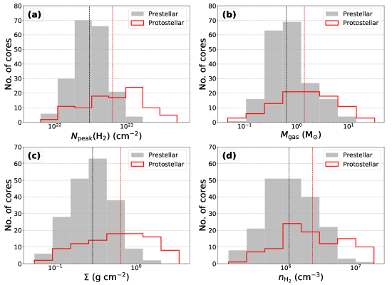
Figure 1: Panels (a)–(d) show the histograms of the peak column density ($N_{\rm peak}$(H₂)), gas mass ($M_{\rm gas}$), surface density ($\Sigma_{\rm H_{2}}$), and volume density ($n_{\rm H_{2}}$) for the prestellar and protostellar cores. The black and red dashed vertical lines indicate the median values of prestellar and protostellar cores, respectively.

3.3 Core Mass and Core Density

We retrieved the rotational excitation temperature ($T_{\rm NH_{3}}$), that is derived from NH₃ (1,1) and (2,2) transition lines (see Appendix B in Li et al., 2022, for detailed procedure on excitation temperature determination), from the Complete ATCA Census of High-Mass Clumps (CACHMC; Allingham et al., 2023, in preparation) at about 5^′′ angular resolution. The retrieved $T_{\rm NH_{3}}$ is used as excitation temperature in the calculation of all molecular parameters and core mass, except for G332.96 that has no available NH₃ data. The dust temperature of 12.6 K derived from the clump scale is used for G332.96 (Sanhueza et al., 2019). The prestellar and protostellar cores have similar $T_{\rm NH_{3}}$, with the median values of 14.1 and 14.8 K for the prestellar and protostellar cores, respectively. These values are lower than the typical gas temperature $\geqslant$ 20 K of protostellar cores reported in previous studies (e.g., Lu et al., 2014; Billington et al., 2019). This further supports the notion that these protostellar cores are still at a very early evolutionary phase. The low temperature in the protostellar cores could be attributed to the fact that these cores are still at a very early evolutionary stage, and the surrounding core materials have not been sufficiently warmed up. On other other hand, we cannot fully rule out the possibility that the NH₃ observations have not enough sensitivity or angular resolution to reveal local small temperature enhancement toward the protostellar cores.

We have updated the gas mass ($M_{\rm gas}$), peak column density ($N_{\rm peak}$(H₂)), volume density ($n_{\rm H_{2}}$), and surface density ($\Sigma=M_{\rm gas}/(\pi r^{2})$) using the temperatures derived from the NH₃ data (see Li et al., 2022). The updated parameters are 0.05–31.66 $M_{\odot}$ for the gas mass, 6.3 $\times$ 10²¹–5.0 $\times$ 10²³ cm^-2 for the peak column density, 1.5 $\times$ 10⁵–1.8 $\times$ 10⁷ cm^-3 for the core-averaged volume density, and 0.05–3.39 g cm^-2 for the core-averaged surface density. The updated parameters are slightly different compared to the previous results using the clump-scale dust temperatures in Sanhueza et al. (2019). The updated parameters of each core are tabulated in Table 2 (see also Figure 1).

3.4 Properties of the Molecular Line Data

Due to the low temperatures ($<$20 K) and high densities ($>10^{5}$ cm^-3) found in cores at early stages of evolution, there is a high level of deuteration due to freeze out of the CO molecules into dust grains (e.g., Caselli et al., 2002; Tan, 2018; Sabatini et al., 2019, 2022; Li et al., 2021). This makes the emission from the N₂D⁺ ($J$=3-2; $n_{\rm crit}=1.7\times 10^{6}$ cm^-3) and DCO⁺ ($J$=3-2; $n_{\rm crit}=1.8\times 10^{6}$ cm^-3) molecules almost exclusively associated to the cold and dense gas toward the cores. Unlike H₂CO and CH₃OH that are associated with more turbulent gas components, N₂D⁺ and DCO⁺ preferentially trace quiescent dense gas (see Li et al., 2022). Therefore, N₂D⁺ and DCO⁺ are excellent tracers of the gas velocity dispersion in cold dense cores, minimizing the contribution from more diffuse intra-clump gas and/or more turbulent gas related to protostellar activity, like, for example, molecular outflows.

To determine the properties of the core envelope, defined as the lower-density gas surrounding a dense core, we used the C¹⁸O emission. C¹⁸O ($J$=2-1; $n_{\rm crit}=9.3\times 10^{3}$ cm^-3) traces lower-density gas; thus by determining the properties of the emission observed in the same line of sight to the cores, we can have an idea of the material that might be associated to the gas surrounding each core, or core envelope.

For each core detected in the continuum, we extracted the core-averaged spectrum of the N₂D⁺, DCO⁺, C¹⁸O, H₂CO, and CH₃OH molecular line emission within the same area defined for each core by the dendrogram technique in Sanhueza et al. (2019). The spectral extraction was done for the images created by combining the 12 and 7 m arrays (hereafter 12m7m or interferometric images), and for the images created by adding the TP array data to the 12m7m dataset via the feathering technique (hereafter 12m7mTP or feathered images). We preformed Gaussian fittings to the core-averaged spectrum for each line, except for N₂D⁺ that is fitted using hyperfine line structures (hfs); the detail fitting processes can be found in Li et al. (2022). The best-fit parameters, including the peak brightness temperature ($I$), the line central velocity ($v_{\rm LSR}$), and observed velocity dispersion ($\sigma_{\rm obs}$ = FWHM_obs/$\rm 2\sqrt{2ln2}$), are presented in Table 3.

The C¹⁸O emission, along the line of sight, presents asymmetric profiles toward some of cores. These line features in our sample can be attributed mostly to multiple velocity components because the C¹⁸O is virtually always optically thin in this sample (see Sabatini et al., 2022), and these multiple velocity components match those of N₂H⁺ ($J$=1-0) and ortho-H₂D⁺ (1_1,0-1_1,1) toward G14.49 (the latter two lines are from Redaelli et al., 2022). In order to fit the C¹⁸O emission associated to the cores, the central velocity derived from the other dense gas tracers (i.e., DCO⁺, N₂D⁺, CH₃OH, or H₂CO) was used to guide the Gaussian fit of the C¹⁸O line.

Table 3 summarizes the properties derived from the Gaussian fit for all cores, and Figure 2 shows examples of the molecular lines emission and the fits for five selected cores.

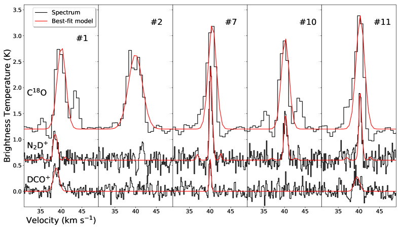
Figure 2: Examples of spectra of C¹⁸O, N₂D⁺, and DCO⁺ for five selected cores in the G14.49. The results of best fit are overlaid on the spectra as red curves.

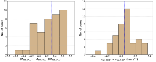
Figure 3: Left panel: histogram of the differences between the velocity dispersion of the DCO⁺ and N₂D⁺ emission. Right panel: histogram of the differences between the $v_{LSR}$ of these two molecules. In both panels, the histogram shows the differences based on the spectra from the 12 and 7 m images. The blue dashed line indicates the median value in each panel.

Table 3: Summary of N₂D⁺ and DCO⁺ lines properties

Clump	Core			N2D+					DCO+
		$T_{a}$	$v_{\rm LSR}$	$\sigma_{\rm obs}$	$\sigma_{\rm nth}$	$\mathcal{M}$	Ta	$v_{\rm LSR}$	$\sigma_{\rm obs}$	$\sigma_{\rm nth}$	$\mathcal{M}$
		(K)	(km s-1)	(km s-1)	(km s-1)		(K)	(km s-1)	(km s-1)	(km s-1)
G10.99	1	0.41(0.03)	29.75(0.03)	0.28(0.03)	0.27(0.03)	1.24(0.14)	0.33(0.03)	29.69(0.05)	0.23(0.12)	0.21(0.13)	0.95(0.61)
G10.99	2	…	…	…	…	…	0.57(0.06)	29.89(0.09)	0.28(0.25)	0.27(0.27)	1.27(1.29)
G10.99	3	0.51(0.05)	29.63(0.05)	0.44(0.05)	0.43(0.05)	2.07(0.25)	0.32(0.03)	29.97(0.13)	0.53(0.38)	0.52(0.39)	2.54(1.88)
G10.99	4	…	…	…	…	…	0.22(0.02)	30.01(0.10)	0.14(0.07)	0.10(0.10)	0.46(0.43)
G10.99	5	0.79(0.11)	29.90(0.03)	0.18(0.03)	0.16(0.03)	0.82(0.22)	0.71(0.07)	29.72(0.06)	0.22(0.13)	0.20(0.15)	1.01(0.77)
G10.99	6	…	…	…	…	…	…	…	…	…	…
G10.99	7	1.74(0.07)	29.56(0.01)	0.19(0.01)	0.17(0.01)	0.82(0.06)	0.55(0.05)	29.41(0.04)	0.18(0.05)	0.15(0.05)	0.73(0.26)
G10.99	8	0.44(0.06)	29.83(0.05)	0.30(0.05)	0.28(0.05)	1.35(0.26)	…	…	…	…	…
G10.99	9	0.66(0.07)	29.52(0.04)	0.35(0.04)	0.34(0.04)	1.69(0.23)	0.56(0.06)	29.46(0.07)	0.20(0.08)	0.17(0.09)	0.87(0.44)
G10.99	10	0.29(0.05)	30.46(0.05)	0.28(0.05)	0.26(0.06)	1.23(0.27)	0.42(0.04)	30.17(0.05)	0.11(0.05)	0.06(0.09)	0.30(0.44)
G10.99	11	0.87(0.16)	29.78(0.03)	0.13(0.02)	0.09(0.04)	0.43(0.18)	…	…	…	…	…

(This table is available in its entirety in a machine-readable form in the online journal. A portion is shown here for guidance regarding its form and content.)

3.4.1 Effects of Combining the Single-dish Observations with the Interferometric Data

We compared the line properties of the spectra obtained from the 12m7m datasets with the 12m7mTP datasets. We found no difference in the $v_{\rm LSR}$ between the spectra for any of the three molecules from the present study (N₂D⁺, DCO⁺, and C¹⁸O), whether we included or excluded TP observations.

For DCO⁺, the spectra obtained from the feathered images have a velocity dispersion $\sigma_{\rm obs}$ on average 10% larger than the spectra obtained from the interferometric data alone. In addition, for 63% of the sample, this difference is lower than 10%. For the N₂D⁺ data, we also see a similar behaviour; however, the differences of $\sigma_{\rm obs}$ between the feathered and nonfeathered data are on average only 3%. This suggests that the DCO⁺ line traces more extended gas than the N₂D⁺ emission toward dense cores.

The largest discrepancy was found for the C¹⁸O velocity dispersion, where the differences between the interferometric data and the one including the single-dish are of the order of $\sim$30%. This is because the C¹⁸O traces relatively lower-density gas compared to the DCO⁺ and N₂D⁺, such as the low-density envelope of cores (Walsh et al., 2004; Tychoniec et al., 2021).

The maximum scale recovered by the 7 m array corresponds to $\sim$0.58 pc (30^′′ at the averaged source distance of 4 kpc), which is much larger than the detected core typical size of $\sim$0.02 pc. Also, the sizes of the cores were determined from their dust continuum emission, which only have the emission from the 12 and 7 m arrays. Therefore to have a better comparison between the properties of the cores and their envelopes, and to avoid the more extended emission that might be associated with the clump itself (intra-clump gas not associated with the dense cores), for the rest of our analyses, we will use the properties of the line emission derived from the data cubes that only contain the 12 and 7 m arrays.

In addition, we have assessed how much flux is recovered in the 12m7m continuum images using the single-dish data retrieved from the APEX ATLASGAL survey at 870 $\mu$m (Schuller et al., 2009). We have scaled the 870 $\mu$m flux to 1.3 mm flux assuming a dust emissivity spectral index of $\beta$ = 1.5; $F_{\rm 1.3mm,exp}=F_{\rm 0.87mm}\,(1.3/0.87)^{-(\beta+2)}$. The continuum images recover about 10–33% ($F_{\rm 1.3mm,12m7m}/F_{\rm 1.3mm,exp}$) of single-dish continuum flux, with a mean value of 21% (see also Sanhueza et al., 2019). For the DCO⁺ and N₂D⁺ lines, their 12m7m data can recover about 79% and 92% of the 12m7mTP flux (see also Li et al., 2022). This suggests that the continuum images recover less extended emission than the DCO⁺ and N₂D⁺ images made using the 12m7m data.

3.5 Gas Properties of the Cores

In general, the emission from the N₂D⁺ and/or DCO⁺ traces well the dust continuum core in the ASHES observations. For the 294 cores detected in the 12 clumps, we detected DCO⁺ emission toward 116 cores (40%) and N₂D⁺ emission toward 54 cores (18%). We detected both DCO⁺ and N₂D⁺ emission toward 41 cores (14%). In total, 129 cores (44%) were detected in either DCO⁺ and/or N₂D⁺.

More than half of dust continuum cores present no detectable emission from either N₂D⁺ or DCO⁺. Comparing the physical properties of the cores with detected and undetected deuterated species, we found that the ones without emission from deuterated species have lower integrated fluxes in their continuum emission ($\langle S_{\rm cont,nodeu}\rangle=1.5$ mJy, compared to $\langle S_{\rm cont,deu}\rangle=4.4$ mJy), smaller masses ($\langle M_{\rm gas,nodeu}\rangle=0.95$ $M_{\odot}$, compared to $\langle M_{\rm gas,deu}\rangle=2.87$ $M_{\odot}$), and lower surface densities ($\langle\Sigma_{\rm nodeu}\rangle=0.36$ g cm^-2, compared to $\langle\Sigma_{\rm deu}\rangle=0.70$ g cm^-2).

Since the emission from the deuterated species is rather weak, with the signal-to-noise in both species going up to 10, the lack of detection of deuterated species could be due to either the sensitivity of our observations or their abundances being too low in the gas phase, or both. Given that we want to compare the properties of the gas and the dust, we only focus on those cores that show emission in both the dust continuum and molecular lines.

The average values of the core line velocity dispersion ($\sigma_{\rm obs}$) are similar in both molecules, with $\sigma_{\rm obs,N_{2}D^{+}}=0.23$ km s^-1 and $\sigma_{\rm obs,DCO^{+}}=0.32$ km s^-1. For the 41 cores that showed emission in both molecules, we compared the observed velocity dispersion ($\sigma_{\rm obs}$) and the central velocity ($v_{\rm LSR}$). Figure 3 shows the differences of these two quantities between DCO⁺ and N₂D⁺. In general, the central velocity differences have a normal distribution centered around 0.05 km s^-1. The DCO⁺ lines are slightly broader than N₂D⁺ lines, which could be due to unresolved hyperfine structure. The velocity dispersion of DCO⁺ is derived from the single Gaussian fit, whereas N₂D⁺ is derived from the hfs fit. In two cases (these two cores are not shown in Figure 3), the central velocity differences are up to 2.10 km s^-1 (G14.49-#6) and 0.77 km s^-1 (G14.49-#11). This is most likely because their local environments have been significantly affected by the nearby strong protostellar outflow (see Figure 1 of Li et al., 2022).

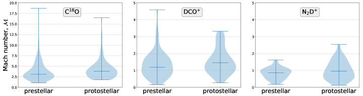
Figure 4: Violin plots of the $\mathcal{M}$ distributions for each line. The shape of each distribution shows the probability density of the data smoothed by a kernel density estimator. The blue horizontal bars from the top to bottom in each violin plot represent the maximum, mean, and minimum values, respectively.

We found that 71% of the cores show a difference in the DCO⁺ and N₂D⁺ central velocity $<0.17$ km s^-1, which is smaller than the spectral resolution of our data, and 94% of all cores shows a difference $<0.34$ km s^-1. Thus, the emission from these two molecules is likely arising from the same physical location in the cores. Therefore, for the analysis of this paper, we will use the velocity dispersion obtained from the DCO⁺ emission, and in the case that DCO⁺ is not detected, we will use the velocity dispersion obtained from the N₂D⁺ line. The measured velocity dispersion have a mean value $\langle\sigma_{\rm obs}\rangle=0.32$ km s^-1, ranging between 0.1 and 0.77 km s^-1. The nonthermal velocity dispersion is given by $\sigma_{\rm nt}^{2}=\sigma_{\rm obs,int}^{2}-\sigma_{\rm th,m}^{2}$, where $\sigma_{\rm obs,int}$ is the intrinsic observed velocity dispersion after removing the smearing effect due to the channel width using $\sigma_{\rm obs,int}=\sqrt{(\rm FWHM_{\rm obs}^{2}-FWHM_{\rm ch}^{2})/8ln2}$ = $\sqrt{\sigma_{\rm obs}^{2}-\rm FWHM_{\rm ch}^{2}/8ln2}$, $\sigma_{\rm obs}$ is the observed velocity dispersion, FWHM_ch is the channel width, and $\sigma_{\rm th,m}=(k_{\rm B}T/\mu m_{H})^{1/2}=9.08\times 10^{-2}\,{\rm km\,s^{-1}}\rm\left(\frac{T}{K}\right)^{0.5}\mu^{-0.5}$ is the thermal velocity dispersion. The value of $\mu$ for both DCO⁺ and N₂D⁺ is 30. The sound speed $c_{\rm s}$ can be estimated using a mean molecular weight per free particle of $\mu_{\rm p}$ = 2.37, which assumes a typical interstellar abundance of H, He, and metals (Kauffmann et al., 2008). For the cores, $\sigma_{\rm th,m}$ ranges between 0.04 and 0.08 km s^-1, with a mean value of 0.06 km s^-1, and $\sigma_{\rm nt}$ ranges between 0.03 and 0.77 km s^-1, with a mean value $\sigma_{\rm nt}=0.27$ km s^-1.

3.6 Gas properties of the envelopes

The C¹⁸O emission is extended and filamentary in the clumps. In our sample, 91% of the cores have C¹⁸O emission, and we speculate that C¹⁸O is likely depleted in the cores where there is no detection (Sabatini et al., 2022). Using the core systemic velocity defined by other dense gas tracers (i.e., N₂D⁺, DCO⁺, H₂CO, or CH₃OH), we were able to fit a Gaussian to the C¹⁸O line profiles to 267 out of the 294 cores. C¹⁸O was observed in a spectral window with coarser spectral resolution (1.3 km s^-1), which is in general still narrower than the derived typical FWHM (2.2 km s^-1) for this transition. However, the coarser spectral resolution might make us overestimate the true internal velocity dispersion of the gas (inside cores). For these reasons, we focused our analysis on the deuterated species, and used the parameters derived from the C¹⁸O only as a reference, to compare the properties of the core’s gas with the properties of their envelopes. The velocity dispersions for the C¹⁸O emission, as expected, have larger values than the ones found for the deuterated species, ranging from $\sigma_{\rm obs,C^{18}O}=0.4$ to 3.4 km s^-1, with a mean value of 0.9 km s^-1.

3.7 Virial mass and virial parameter

To determine the gravitational state of the cores, we calculated their virial parameter $\alpha=M_{\rm vir}/M_{\rm gas}$, where $M_{\rm vir}$ is the virial mass, and $M_{\rm gas}$ is the mass derived from the dust continuum emission. The virial parameter, $\alpha$, is commonly used to assess the gravitational state of molecular clouds. A value of $\alpha<1$ suggests that a core is gravitationally unstable to collapse, and turbulence alone cannot maintain its stability (Bertoldi & McKee, 1992). Nonmagnetized cores with $\alpha\sim 1$ and $\alpha<2$ are considered to be in hydrostatic equilibrium and gravitationally bound, respectively. A value of $\alpha>2$, on the other hand, suggests that the core is gravitationally unbound (Kauffmann et al., 2013), and if we ignore additional support mechanisms such as the magnetic field or external pressure, then the core might be a transient object.

The virial mass was calculated using the observation measurements following (Bertoldi & McKee, 1992):

$$M_{\rm vir}=\frac{5}{a\beta}\frac{\sigma_{\rm tot}^{2}R}{G},$$ (1)

where $R$ is the core radius, $a=(1-b/3)/(1-2b/5)$ is the correction factor for a power-law density profile $\rho\propto R^{-b}$, $\beta=({\rm arcsin}\,e)/e$ is the geometry factor (see Fall & Frenk, 1983; Li et al., 2013, for detailed derivation), $\sigma_{\rm tot}$ is the total velocity dispersion of the gas in the core, and $G$ is the gravitational constant. The eccentricity $e=\sqrt{1-f_{\rm int}^{2}}$ is calculated by the intrinsic axis ratio, $f_{\rm int}$, of the dense cores. The $f_{\rm int}$ can be estimated from observed axis ratio, $f_{\rm obs}$, with $f_{\rm int}=\frac{2}{\pi}\,f_{\rm obs}\,\mathcal{F}_{1}(0.5,0.5,-0.5,1.5,1,1-f_{\rm obs}^{2})$ (Fall & Frenk, 1983), where $\mathcal{F}_{1}$ is the Appell hypergeometric function of the first kind. For the dense cores, the derived $\beta$ ranges from 1.0 to 1.4, with a mean value of 1.2. Here we adopted a typical density profile index $b=1.6$ for all dense cores (e.g., Beuther et al., 2002; Butler & Tan, 2012; Palau et al., 2014; Li et al., 2019). The velocity dispersion is given by $\sigma_{\rm tot}^{2}=\sigma_{\rm nt}^{2}+c_{\rm s}^{2}$, and it reflects a combination between the nonthermal motions of the gas within the core, $\sigma_{\rm nt}$, and the thermal motion of the particle mean mass, $c_{\rm s}^{2}$. $c_{\rm s}^{2}$ ranges between 0.16 and 0.28 km s^-1, with a mean value of 0.23 km s^-1.

We found that the values of the virial masses range from 0.22 to 8.61 $M_{\odot}$, and the mean value is 1.89 $M_{\odot}$ for all the 129 cores analyzed. The virial parameter $\alpha=M_{\rm vir}/M_{\rm gas}$ ranges from 0.15 to 8.91, with a mean value of 1.39. Seventy-three out of 129 cores have virial parameters below 1, 28 cores have virial parameters between 1 and 2, and 28 cores have $\alpha$ larger than 2. The derived values of the virial mass and virial parameter are summarized in Table 2.

Table 4: Median and mean values of derived core properties for each category

Name	Prestellar		Protostellar								All
			Outflow Core		Warm Core		Warm&outflow Core		Suma
	Median	Mean	Median	Mean	Median	Mean	Median	Mean	Median	Mean	Median	Mean
$T_{\rm NH_{3}}$	14.1	14.2	12.8	13.8	14.8	14.3	15.3	14.9	14.8	14.4	14.4	14.3
$M$	0.63	1.15	1.26	2.18	0.69	2.00	3.11	4.66	1.41	3.11	0.77	1.79
$n_{\rm H_{2}}$	1.11	1.58	1.59	2.62	1.26	2.82	3.59	5.55	2.40	3.87	1.32	2.34
$N_{\rm peak}$(H2)	3.01	3.58	5.40	7.26	3.35	5.55	11.40	15.57	6.32	9.95	3.58	3.73
$\Sigma$	0.29	0.34	0.46	0.60	0.30	0.54	0.96	1.27	0.64	0.85	0.35	0.51
$R$	0.012	0.014	0.014	0.015	0.012	0.013	0.013	0.015	0.013	0.014	0.013	0.014
$M_{\rm vir}$	1.05	1.67	1.31	1.33	1.28	2.29	2.00	2.42	1.58	2.18	1.25	1.89
$\alpha$	1.01	1.54	0.52	0.61	1.88	2.35	0.40	0.53	0.58	1.19	0.87	1.39
$\mathcal{M}_{\rm N_{2}D^{+}}$	0.9	0.8	1.0	1.1	0.8	0.9	1.0	1.0	0.9	1.0	0.9	1.0
$\mathcal{M}_{\rm DCO^{+}}$	1.2	1.3	1.4	1.3	1.6	1.7	1.5	1.5	1.5	1.6	1.3	1.4
$\mathcal{M}_{\rm C^{18}O}$	3.1	3.8	3.8	4.2	4.0	4.4	3.6	4.0	3.8	4.2	3.3	3.9

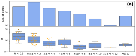
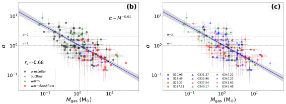
Figure 5: Panel (a): upper panel shows the number of sources per mass bin, and the bottom panel shows a box plot of the values of the virial parameter per bin. In the box plot, the mean value of the virial parameter is shown with a horizontal line. Panels (b) and (c): $\alpha$ versus mass for all the cores where molecular emission from either N₂D⁺ or DCO⁺ was detected. Panel (b) shows the cores color coded by their evolutionary stage classification (Li et al., 2022), and panel (c) shows the cores color coded by their parental molecular cloud. The solid line in both figures shows the linear regression to all the point in the plot, gives a slope of -0.61 $\pm$ 0.06, and the gray shadowed area shows the 1$\sigma$ confidence interval for the fit. The Spearman’s rank test returns a coefficient of $r_{s}$ = -0.68.

3.8 Mach Number

To analyze the amount of turbulence within the cores, we calculated the one-dimensional (1D) turbulent Mach number ($\mathcal{M}=\sigma_{\rm nt}/c_{\rm s}$). The $\mathcal{M}$ shows no significant difference between the prestellar and protostellar cores for C¹⁸O, DCO⁺, and N₂D⁺ (see Figure 4), indicating that the nonthermal motions of the molecular gas traced by C¹⁸O, DCO⁺, or N₂D⁺ have not yet been significantly influenced by protostellar activity. There are 98% (53/54) and 82% (95/116) of $\mathcal{M}$ derived from N₂D⁺ and DCO⁺ smaller than 2, respectively. N₂D⁺ and DCO⁺ are typical tracers of cold and dense gas that are closely related to core formation. The transonic $\mathcal{M}$ suggests that the cold and dense gas in the cores have been so far weakly affected by protostellar feedback (see also Li et al., 2020b), albeit a small fraction (14%) of embedded cores is associated with outflow activity. Therefore, these 70 $\mu$m dark clumps are ideal targets for investigating the initial conditions of massive star and cluster formation.

Overall, $\sigma_{\rm obs}$ and $\mathcal{M}$ of C¹⁸O are systemically higher than N₂D⁺ and DCO⁺. This is because the latter two deuterated species are preferentially tracing cold and dense gas, whereas C¹⁸O probes relatively less dense gas.

For all cores, the $\mathcal{M}$ derived from DCO⁺ or N₂D⁺ ranges from 0.1 to 4.6, with the mean and median values of 1.4 and 1.3, respectively. We found that 44 cores show subsonic motions ($\mathcal{M}\leqslant$1), and 64 cores present transonic motions (1$<\mathcal{M}\leqslant$2). This suggests that the motions in most of the deuterated cores (108/129 = 84%) are subsonic or transonic dominated.

4 Discussion

4.1 Core mass growth

As shown in Figure 1, the protostellar cores have higher column densities, gas masses, volume densities, and surface densities than those from prestellar cores (see also Table 4). A similar trend is found in the individual clumps, except for G331.37, G340.17, and G340.22. The latter two clumps are still at very early evolutionary phases as evidenced by the nondetection of molecular outflows. The G331.37 hosts 1 relatively massive (7.96 $M_{\odot}$) prestellar core, while the rest of the prestellar and protostellar cores have comparable mass ($<$ 4 $M_{\odot}$).

These results suggest that the protostellar cores are more massive and denser than the prestellar cores, indicating a core mass growth from the prestellar to protostellar stages (e.g., Kong et al., 2021; Takemura et al., 2022; Nony et al., 2023). In addition, Li et al. (2020b) found that the more massive cores have a longer accretion history than the less massive cores. A Kolmogorov-Smirnov (KS) test, which returns a probability ($p$-value) of two samples being drawn from the same population, was used to compare the peak column density, gas mass, volume density, and surface density of the prestellar cores with those of the protostellar cores. If the $p$-value is much smaller than 0.05, we can reject the null hypothesis that the two samples are drawn from the same parent distribution (Teegavarapu, 2019). The KS test reveals that the $p$-value is 2.5$\times$10^-13, 1.6$\times$10^-6, 1.6$\times$10^-6, and 6.8$\times$10^-12 for peak column density, gas mass, volume density, and surface density, respectively, indicating that the prestellar cores and the protostellar cores in our sample are drawn from significantly different populations ($p$-value $\ll$ 0.05).

Table 4 also shows that warm and outflow cores tend to be more massive and denser than the remaining type of cores. The warm and outflow cores associated with molecular outflows and warm line(s) emission could be considered as the most evolved objects among the identified cores. This further supports that the cores have grown in mass and density over time.

4.2 Stability

Several observational biases could lead to underestimate the virial parameter. For instance, the observed line width could be underestimated when a particular molecular line preferentially traces molecular gas with densities above the critical density of the line transition, resulting in an underestimation of the virial parameter (Traficante et al., 2018b). In our case, this effect is likely insignificant owing to the critical density of the transition lines used in this study typically being 1-2 orders of magnitude larger than the effective excitation density because of the effect of radiative trapping (Shirley, 2015); the critical density is $\sim$10⁶ cm^-3 for DCO⁺ and N₂D⁺. Therefore, both DCO⁺ and N₂D⁺ can effectively trace dense gas within the cores. On the other hand, the virial parameter could be overestimated if gas bulk motions and background emission are not properly considered in the calculation of the velocity dispersion (e.g., Singh et al., 2021). We computed the velocity dispersion from the core-averaged spectrum for each core, bulk motions (if present) already included as they could increase the velocity dispersion over the core. In addition, the interferometric observations of dense gas tracers filter out the large-scale emission and, therefore, are barely affected by the contamination of background emission. Overall, the above-mentioned observational biases do not significantly affect our results.

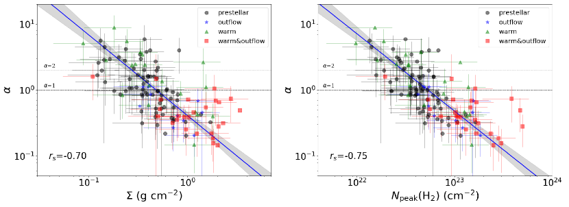
Figure 6: Left panel: virial parameter versus surface density. Right panel: virial parameter versus peak column density. The blue solid line in both figures shows the linear regression to all the point in the plot, and the gray shadowed area shows the 1$\sigma$ confidence interval for the fit. The best fit gives a slope -1.22 $\pm$ 0.15 and -1.17 $\pm$ 0.13 for $\alpha$–$\Sigma$ and $\alpha$–$N_{\rm H_{2}}$, respectively. The Spearman’s rank coefficients are shown in the lower left of each panel.

4.2.1 Are massive cores more unstable?

Comparing the virial parameter of the cores with their masses, we find a correlation between these two quantities. The value of $\alpha$ appears to decrease with increasing core mass (see Figure 5), with a Spearman’s rank correlation coefficient of $r_{s}$ = -0.68 ($p$-value=1.7$\times 10^{-18}$). Considering that the virial parameter is mathematically inversely proportional to the cores’ mass, a slope of -1 in a log–log plot would suggest that the trend seen is not physically meaningful. A linear regression between the $\log{\alpha}$ and $\log{M_{\rm gas}}$, gives a slope of -0.61 $\pm$ 0.06, indicating that the trend between the stability of the cores and their mass is real, and not due to an observational bias given by the correlation between the two core properties. The observed trend of $\alpha$ and $M_{\rm gas}$, $\alpha\sim M_{\rm gas}^{-0.61\pm 0.06}$, is consistent with the expectations for pressure-confined cores, in which $\alpha$ should depend on mass as $\alpha\sim M_{\rm gas}^{-2/3}$ (e.g., Bertoldi & McKee, 1992). The $\log{\alpha}-\log{M_{\rm gas}}$ correlation indicates that the most massive cores tend to be more gravitationally unstable. In contrast, the less massive cores are gravitationally unbound and may eventually disperse if no other mechanism(s) can help to confine them, such as external pressure (Li et al., 2020a). A similar inverse relationship between the virial parameter and the core mass has also been seen in other IRDCs (e.g., Li et al., 2019, 2020a).

As shown in Figure 6, there is a strong inverse relationship between the virial parameter and the core surface density, with a Spearman’s rank coefficient of $r_{s}$ = -0.70 ($p$-value=6.4$\times 10^{-20}$), and the best fit returns a slope of -1.22 $\pm$ 0.15. This indicates that higher surface density cores appear to be more gravitationally unstable. We also find a strong trend of virial parameters and column density, with the higher column density tending to show a lower virial parameter (see Figure 6). The Spearman’s rank test returns a coefficient of $r_{s}$ = -0.75 ($p$-value=1.8$\times 10^{-24}$), and the best fit gives a slope of -1.17 $\pm$ 0.13. The inverse $\alpha-N_{\rm H_{2}}$ relation suggests that the higher-density cores tend to be more gravitationally unstable. Overall, these results suggest that the more massive and denser cores tend to be more gravitationally unstable.

Given the angular resolution of our observations, it is possible that with observations at higher angular resolution the most massive cores could further fragment into smaller objects. Assuming that the cores are not fragmented, and ignoring the effect of additional support (such as magnetic fields), we suggest that cores with masses M${}_{\rm core}>4$ $M_{\odot}$ in each clump are strongly self-gravitating ($\langle\alpha\rangle\,=0.37<1$) and prone to collapse, except for core #8-G28.27, #1-G332.96, and #4-G340.22 that have $\alpha$ of 1.6, 1.4, and 1.1, respectively.

The most massive core in all the 12 IRDCs is core #1 in G340.23, with a mass of 31.66 $M_{\odot}$. For the remaining IRDCs, the most massive cores have masses of $\sim$10 $M_{\odot}$. If these cores will form high-mass stars, then while collapsing they might still be accreting material from their environment in order to have enough mass ($>27$ $M_{\odot}$, assuming a star formation efficiency of 30%) to form a $>$8 $M_{\odot}$ star. Indeed, this is happening for one of the cores of G331.37 (core #1), where additional observations of the HCO⁺ molecular gas show that this subvirialized core is accreting material at a high rate from its environment (Contreras et al., 2018). If this core in G331.37 continues to accrete at its current rate ($2.0\times 10^{-3}$ $M_{\odot}$ yr^-1), it is expected that in a freefall time (3.3 $\times$ 10⁴ yr) the core will have 82 $M_{\odot}$, gathering a large mass reservoir and allowing the formation of high-mass stars. Although this is only one example, we may expect similar accretion rates in several ASHES cores given their low virial parameters and massive gas reservoir in their natal clumps (see Table 1). In addition, the filamentary structures connected to cores can also transport material from the parental clump onto cores and thus further increase their masses. For example, the mass flow rate along a filamentary structure feeding a protostellar core in one of the ASHES targets, G14.49, is about $2.2\times 10^{-4}$ $M_{\odot}$ yr^-1 (Redaelli et al., 2022). Such accretion rates along filamentary structures are not unusual in high-mass star-forming regions (e.g., Sanhueza et al., 2021).

4.2.2 Does core stability change with the evolutionary stage of cores?

Prestellar and protostellar cores have a mean virial mass of $\langle M_{\rm vir}\rangle=1.67$ $M_{\odot}$ and $\langle M_{\rm vir}\rangle=2.18$ $M_{\odot}$, respectively. Overall, protostellar cores have higher virial mass than that of prestellar cores, indicating that the virial mass tends to increase with the evolutionary stage of cores. This is likely because the velocity dispersion toward protostellar cores is slightly larger than that of prestellar cores; the mean velocity dispersion derived from N₂D⁺ or DCO⁺ is 0.28 and 0.32 km s^-1 for prestellar and protostellar cores, respectively. On the other hand, the virial parameter of protostellar cores is slightly lower than the prestellar cores as shown in Figure 5. The prestellar cores have a mean virial parameter of $\langle\alpha\rangle=1.5$, while the protostellar cores have a mean value of $\langle\alpha\rangle=1.2$. This is because the protostellar cores have relatively higher gas mass than the prestellar cores. The lower value of the virial parameter, ignoring additional forces of support, for protostellar cores is in agreement with the scenario where protostars might be embedded in them, and thus the gravitational collapse has already started in these regions. Figures 5 and 6 suggest that the virial parameter decreases with mass and density. In Section 4.1, we also find that both mass and density of cores increase from the prestellar to the protostellar phase. These observational results indicate that the virial parameter tends to decrease with the evolutionary stage of cores, and therefore cores become more gravitationally unstable with evolution.

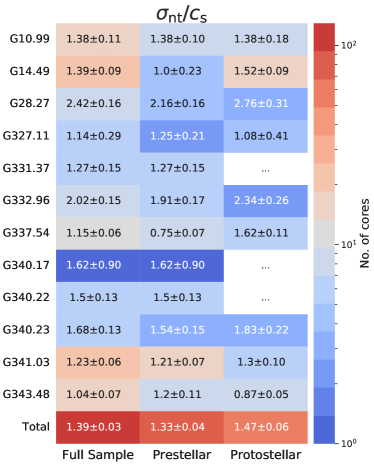
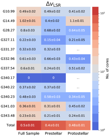
Figure 7: Left panel: the Mach number ($\sigma_{\rm nt}/c_{\rm s}$) of the cores, obtained from DCO⁺ or N₂D⁺ molecular line emission for each clump. The total row shows the mean value of the velocity dispersion for the clumps that have a measurement in both the prestellar and protostellar sample. Right panel: core-to-core velocity dispersion of the cores $v_{\rm LSR}$ obtained from DCO⁺ or N₂D⁺ molecular line emission for each clump. The total row shows the mean value of the core-to-core velocity dispersion for the clumps that have a measurement in both the prestellar and protostellar sample. The color scale shows the number of cores considered to determine the velocity dispersion. ‘0’ means only one available core. Dashes denote no available core.

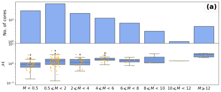
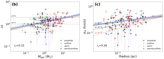
Figure 8: Panel (a): upper panel shows the number of sources per mass bin, and the bottom panel shows a box plot of the values of the Mach number per bin. In the box plot the mean value of the Mach number is shown with a horizontal line. Panel (b): Mach number versus mass for all the cores where molecular emission from N₂D⁺ or DCO⁺ was detected. The blue solid line shows the linear regression to all the points in the plot (slope of 0.17 $\pm$ 0.04) and the gray shadowed area shows the 1$\sigma$ confidence interval for the fit. The Spearman’s rank test gives a coefficient of $r_{s}$ = 0.33, suggesting a moderate correlation between Mach number and gas mass. Panel (c): nonthermal velocity versus core radius for all the cores where molecular emission from N₂D⁺ or DCO⁺ was detected. The correlation between nonthermal velocity and core radius is weak, with a spearman’s rank coefficient of $r_{s}$ = 0.28. The black dashed line shows the the original Larson relation with $\sigma\propto R^{0.38}$ (Larson, 1981), and the red dashed line is the revised Heyer & Brunt (2004) relation with $\sigma\propto R^{0.56}$. The blue solid line indicates the best fitting result with $\sigma\propto R^{0.27}$.

4.3 Turbulence

4.3.1 Global turbulence in IRDCs

The origin of turbulence in molecular clouds is still not well understood, as well as its behavior with cloud evolution. Molecular cloud formation and destruction can be a dynamical process, in which turbulence is transient, decaying quickly on timescales comparable to the cloud lifetime (e.g., Elmegreen, 2000; Hartmann, 2001; Dib et al., 2007). Alternatively, the turbulence can decay slowly in a quasi-equilibrium process, in which turbulence is fed into the molecular cloud by, for example, protostellar outflows, HII regions, or external cloud shearing (e.g., Shu et al., 1987; McKee, 1999; Krumholz & Bonnell, 2007; Nakamura & Li, 2007).

Simulations of isothermal molecular clouds with and without a continuous injection of energy have shown differences in the properties of the core gas internal velocity dispersion and the relative motions (i.e., the core-to-core centroid velocity dispersion) between the cores (Offner et al., 2008a, b). Therefore, observations of these properties can in principle be used to analyze the degree of turbulence within molecular clouds.

In the driven scenario, i.e., where there is a continuous injection of energy into the cloud, the simulations show that, in a clump, prestellar cores have in average $\sigma_{\rm nt}<1.5c_{\rm s}$, and there is a small increment of this value for protostellar cores (Offner et al., 2008b, a). In the decay scenario, where there is no additional injection of energy to the cloud, prestellar cores have in average $\sigma_{\rm nt}<1.0c_{\rm s}$, and it increases to larger values for protostellar cores (Offner et al., 2008b, a). This is because, as the turbulence decays, the cloud will start to collapse, and material will fall into the clump gravitational potential.

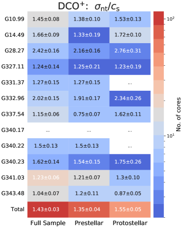
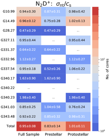
Figure 11: Nonthermal velocity dispersion of the cores $\sigma_{\rm nt}$, obtained from their DCO⁺ (left) and N₂D⁺ (right) molecular line emission for each clump. The total row shows the mean value of the velocity dispersion for the clumps that have a measurement in both the prestellar and protostellar sample. The color scale shows the number of cores considered to determine the velocity dispersion. Dashes denote no available core.

In our observations, the mean velocity dispersion, derived from the N₂D⁺ or DCO⁺, between the prestellar and protostellar cores increases slightly from $\sigma_{\rm nt}\sim(1.33\pm 0.04)c_{\rm s}$ to $\sigma_{\rm nt}\sim(1.47\pm 0.06)c_{\rm s}$. This trend is also seen in 7 out of 9 clumps that have available $\sigma_{\rm nt}$ from N₂D⁺ or DCO⁺. G327.11 and G343.48 do not show this trend. There are three clumps (G331.37, G340.17, G340.22) with no available $\sigma_{\rm nt}$ from N₂D⁺ or DCO⁺ for the protostellar sample. The velocity dispersion in the protostellar cores is similar or slightly smaller than those of prestellar cores in the latter two clumps. In addition, the mean velocity dispersion obtained from C¹⁸O also shows a small increment from prestelllar to protostellar stages in a clump. The statistics for the velocity dispersion of DCO⁺ and N₂D⁺ for each clump are presented in Appendix A (see Figure 11). Overall, the measured core-averaged $\sigma_{\rm nt}$ does not increase significantly from prestellar to protostellar phases, suggesting that our observations are consistent with simulations where there is a continuous injection of energy, consistent with the driven scenario.

An additional piece of information can be obtained by studying the core-to-core velocity dispersion. For simulations where no additional sources of turbulence are injected, and therefore the turbulence is decaying, the relative motions between protostellar cores have a higher dispersion compared to the prestellar cores (Offner et al., 2008b). On the other hand, if the turbulence is driven, i.e., energy is continuously injected into the simulations, the prestellar cores have a higher core-to-core velocity dispersion than the protostellar cores (Offner et al., 2008b).

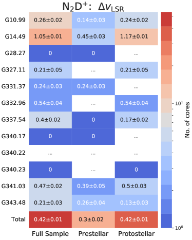
Figure 12: Core-to core velocity dispersion of the cores $v_{\rm LSR}$ obtained from their DCO⁺ (left) and N₂D⁺ (right) molecular line emission for each clump. The total row shows the mean value of the core-to-core velocity dispersion for the clumps that have a measurement in both the prestellar and protostellar sample. The color scale shows the number of cores considered to determine the core-to-core velocity dispersion. ‘0’ means only one available core. Dashes denote no available core.

The core-to-core velocity dispersion ($\Delta v_{\rm LSR}$) is computed from the standard deviation of the centroid velocity ($v_{\rm LSR}$) of all of the dense cores within each clump. The calculations were performed for clumps having more than two core centroid velocities available. We calculated the core-to-core centroid velocity dispersion between the cores for each clump from the $v_{\rm LSR}$ of the Gaussian fits to the DCO⁺ and N₂D⁺ emission. Figure 7 shows a heat-map of the velocity dispersion for all the cores, and for the cores classified as prestellar and protostellar. We find that in three clumps the core-to-core velocity dispersion is comparable between protostellar and prestellar cores (i.e., G28.27, G343.48, and G327.11), which is neither consistent with the driven nor the decaying turbulence simulations. The core-to-core velocity dispersion of prestellar cores is higher than that of protostellar cores in three clumps (i.e., G10.99, G332.96, and G340.23), which is consistent the driven turbulence scenario. On the other hand, we also find that the core-to-core velocity dispersion of prestellar cores is smaller than that of protostellar cores in other three clumps (i.e., G14.49, G337.54, and G341.03), which is consistent with the decaying turbulence scenario. The core-to-core velocity dispersion variation among the clumps might reflect differences in their internal turbulence, which possibly varies clump by clump and/or related to the local cloud environments. The statistics for the core-to-core velocity dispersion derived from DCO⁺ and N₂D⁺ for each clump are presented in Appendix A (see Figure 12). Overall, the prestellar cores have a smaller core-to-core velocity dispersion compared to the protostellar cores if we take the mean value of all the ASHES clumps (Figure 7).

The observations presented here, corresponding to the pilot survey (Sanhueza et al., 2019), give some support to the scenario in which the global turbulence of IRDCs is driven, but a larger sample is required before to draw firm conclusions on the relative merits of driven or decaying turbulence. We expect to address this point again using the complete survey in the future.

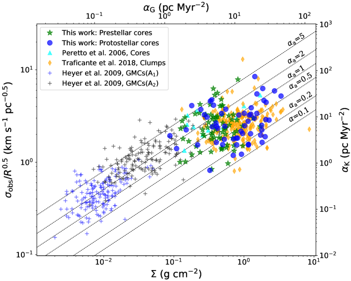
Figure 9: Modified Larson relationship, also called Heyer relationship, between the cloud line widths, radius, and surface density. Top and right axes express the same quantities in term of acceleration parameters ($a_{G},a_{K}$). Green stars and blue circles show the prestellar and protostellar cores, respectively. Cyan triangles present the values for the dense cores in high-mass star formation regions (Peretto et al., 2006). Diamonds show the values for the massive 70 $\mu$m dark clumps (Traficante et al., 2018a). Crosses present the values obtained for the GMCs in the Galactic plane (Heyer et al., 2009).

4.3.2 Turbulence within the cores

To determine the turbulence of the gas within the cores, we analyzed the nonthermal velocity dispersion of the molecular emission detected from each core, and their Mach number (see Section 3.8).

The Mach number, which provides an indication of the level of gas turbulence, shows a moderate positive correlation with the mass of the cores (see panel (b) of Figure 8), with a Spearman’s rank correlation of $r_{s}$ = 0.33 ($p$–value=1$\times 10^{-4}$). A similar positive correlation has also been seen in the IR-dark, high-mass star-forming region NGC6334S (Li et al., 2020a). Also, there is a small increment (11%) in the mean Mach numbers from prestellar cores, with $\langle\mathcal{M}\rangle=1.33\pm 0.04$, to protostellar cores, with $\langle\mathcal{M}\rangle=1.47\pm 0.06$.

The nonthermal velocity dispersion derived from the deuterated species also slightly increases from the prestellar to the protostellar stage. The variation is small (14%) from the prestellar cores, with ($\langle\sigma_{\rm nt}\rangle=0.28$ km s^-1), to the protostellar cores, with ($\langle\sigma_{\rm nt}\rangle=0.32$ km s^-1). The nonthermal velocity dispersion of the envelope traced by C¹⁸O remains essentially the same, with only a small variation of 12%, between the prestellar ($\langle\sigma_{\rm nt,C^{18}O}\rangle=0.83$ km s^-1) and protostellar ($\langle\sigma_{\rm nt,C^{18}O}\rangle=0.93$ km s^-1) cores. This suggests that the variation of turbulence within the cores from the prestellar to the protostellar phase is negligible in the very early stages of high-mass star formation studied in ASHES, likely because not enough time has passed from the protostellar cores to inject turbulence into the surrounding medium (core and envelope). This is consistent with the outflow analysis made on the ASHES sample by Li et al. (2020b); they presented a detailed study of the energy input given by the outflows and found that the outflow-induced turbulence contribution to the internal clump turbulence at the current epoch is very limited.

Studies from more evolved high-mass star-forming regions (e.g., Sánchez-Monge et al., 2013), however, have shown larger differences between the prestellar and protostellar cores’ line widths ($\sim$80% differences); the mean observed velocity dispersion is 0.42 and 0.76 km s^-1 for the prestellar and protostellar cores, respectively. Larger values seen in more evolved objects seem to be associated with the effect of turbulence injected by outflow activity (e.g., Liu et al., 2020b). This difference could be explained by the fact that the ASHES IRDCs are in a very early stage of evolution (70 $\mu$m dark), and what we define as protostellar cores in this sample corresponds to an intermediate stage, between prestellar cores and more evolved protostellar cores that already have significant emission at infrared wavelengths. This suggests that the outflow of these early protostellar cores is not yet significantly affecting the turbulence within the cores (see also Li et al., 2020b).

The lack of a significant increment in the turbulence within the cores as they evolve suggests that the star formation activity in our protostellar cores is very recent (see also Figure 7). It is likely that the effect of the new, recently formed protostars have not had sufficient time and sufficient energy to considerably affect their natal cocoons at the core scale (a few 1000 au), and their effect may be localized at much smaller scales than those we can resolve with the current observations. The massive cores tend to have larger radii (see Figure 14), whereas the nonthermal velocity dispersion has no significant change with the core radius (see Figure 8). This suggests that the larger Mach number found in the massive cores is not because of the spectrum averaged over the larger core radius. Therefore, the increase in turbulence with the core mass might not be the result of core evolution, but rather a natural difference between low- and high-mass cores. The high-mass cores show relatively lower virial parameters, indicating that the high-mass cores would need additional support, even though it is not sufficient to maintain equilibrium, to counterbalance gravity, slowing down the collapse on times larger than the free-fall time.

4.3.3 Are observed line widths dominated by gravitational collapse?

If a cloud is undergoing global gravitational collapse, then the line widths can be dominated by the inward motions produced by this collapse. This can happen at both cloud and/or core scales (Vázquez-Semadeni et al., 2009; Ballesteros-Paredes et al., 2011). Indeed, Heyer et al. (2009) showed that the dynamics of molecular clouds can be dominated by the global gravitational collapse and presented a scaling relation that extends the initial relation of Larson (1981), between the clumps’ line velocity dispersion and radius. The scaling relation proposed by Heyer et al. (2009) shows that the ratio $\sigma/R^{0.5}$ is proportional to the surface density, $\Sigma$, of the clouds.

The effect of the global collapse on the nonthermal motions can be estimated by a gravitational parameter that depends on the surface density ($\Sigma$) of the cloud and/or core, $a_{\rm G}=\pi G\Sigma/5$, compared to a kinetic parameter that depends on the line width ($\sigma$) and radius (R) of the cloud and/or core $a_{\rm K}=\sigma_{\rm tot}^{2}/R$ (Traficante et al., 2018a). These two parameters are related to a virial parameter ($\alpha_{a}$) via $a_{\rm K}=\alpha_{\rm a}a_{\rm G}$, whose interpretation is different than the usual virial parameter derived from the ratio between virial mass and total gas mass (Section 3.7). If the gravitational collapse dominates over the kinetic energy in the cloud, then $a_{\rm K}<a_{\rm G}$.

We computed these parameters for the clumps and their embedded cores from the ASHES survey, and compared them with the values found by Traficante et al. (2018c) in a sample of clumps, by Peretto et al. (2006) for a sample of cores embedded in a high-mass star-forming region, and by Heyer et al. (2009) for a sample of giant molecular cloud (GMC) in the Galactic plane (see Figure 9), which includes GMCs (A₁) and their high-density area within 1/2 maximum isophote of H₂ column density (A₂).

There are 47 out of 129 cores with a value of $\alpha_{a}$ smaller than 1 in the ASHES survey. In general, the cores have values of $a_{\rm G}$ and $a_{\rm K}$ leading to values of $\alpha_{\rm a}$ between 0.1 and 5.0, and the dense clumps have a similar distribution. On the other hand, the GMCs have relatively larger $\alpha_{\rm a}$ compared to the clumps and the cores.

To determine any real correlation, we calculated the Spearman’s correlation coefficient between $\sigma_{\rm obs}/R^{0.5}$ and $\Sigma$ (or $a_{\rm G}$ and $a_{\rm K}$) for the prestellar and protostellar cores. The correlation coefficient for prestellar cores is $r_{s}$ = 0.05 ($p$–value=0.65), suggesting that there is no linear correlation between these values. For protostellar cores, the value of the correlation coefficient is $r_{s}$ = 0.27 ($p$–value=0.04), suggesting a moderate linear trend. This suggests that for prestellar cores the observed line widths are not dominated by gravity. However, once star formation begins, the gravitational collapse plays a role in the dynamics of the cores and thus contributes to the line widths. This is also consistent with the low value of the “standard” virial parameter found for the protostellar cores in which the role of gravitational potential energy with respects to the kinematic energy becomes more important (Section 4.2.2).

4.3.4 The first Larson relation: velocity dispersion-size relation

Larson (1981) found an empirical power-law relationship between global velocity dispersion, $\sigma_{\rm obs}$ (km s^-1), and cloud size, $R$ (pc), of molecular clouds, with a slope of 0.38, $\sigma_{\rm obs}\propto R^{0.38}$. This correlation resembles the turbulent cascade of energy, and thus, it is considered as an indication that turbulence dissipates from large spatial scale down to smaller spatial scales. The $\sigma_{\rm obs}$–$R$ relation has also been found in the other studies of different molecular clouds, but with a different slope (e.g., 0.56; Heyer & Brunt, 2004). On the other hand, the relation seems to break in some studies of star-forming regions, either with a significantly lower slope, e.g., $\sigma_{\rm obs}\propto R^{0.21}$ obtained from Orion A and B (Caselli et al., 1995), or without correlation (Plume et al., 1997; Ballesteros-Paredes et al., 2011; Traficante et al., 2018a).

To explore the variation of $\sigma_{\rm obs}$–$R$ relation in different spatial scales, we have retrieved data from Li et al. (2020a) and Lu et al. (2018) for a sample of embedded cores in high-mass star-forming regions, from Ohashi et al. (2016) for a sample of high-mass clumps and embedded cores, from Traficante et al. (2018c) for a sample of high-mass clumps, and from Heyer et al. (2009) for a sample of GMCs. From the top panel of Figure 10, we note that there is a weak correlation ($r_{s}$ = 0.27, and $p$–value=0.002) between $\sigma$ and R for ASHES cores only, with a slope of 0.24 $\pm$ 0.08 that is similar to the values of 0.2–0.3 reported in Caselli et al. (1995) and Shirley et al. (2003). For ASHES cores only, the sample covers a limited range of radii, which could break down the $\sigma_{\rm obs}$–$R$ relation.

As shown in the middle panel of Figure 10, if the clumps and relatively larger size cores are included, the $\sigma_{\rm obs}$ and $R$ show a strong correlation ($r_{s}$ = 0.82, and $p$–value=4.5$\times 10^{-114}$), with a slope of 0.46 $\pm$ 0.01 that is between 0.38 and 0.56. On the other hand, if the GMCs are included, the correlation between $\sigma_{\rm obs}$ and R becomes even stronger ($r_{s}$ = 0.88, and $p$–value=2.7$\times 10^{-208}$), but however, the slope (0.35 $\pm$ 0.01) becomes more flattened. The change in the slope between including or excluding GMCs could be due to intrinsic turbulent variation from GMC scale to clump and/or core scale or observational bias since the measurements are obtained with different molecular lines and different kind of telescopes. The GMCs values were derived from ¹³CO, while clumps and/or cores were obtained from more dense gas tracers (i.e., NH₃, DCO⁺, and N₂D⁺). Unfortunately, we can not conclude which effect drives the variation in the slope.

Overall, our results suggest that the relation between $\sigma_{\rm obs}$ and $R$ persists from GMC scale down to core scale (Figure 10), and the slope is between 1/3 and 1/2, the former is expected for turbulence-dominated solenoidal motions, and the latter expected for shock-dominated turbulence (Kolmogorov, 1941; Galtier & Banerjee, 2011; Federrath, 2013). Our results also indicate that caution is required in interpreting the investigation of a sample with a small range of radii because it could break down the $\sigma_{\rm obs}$–$R$ relation due to the small dynamical range in the spatial size.

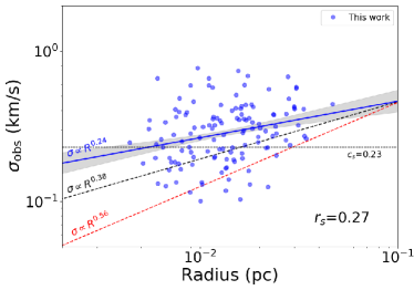
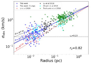
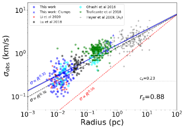
Figure 10: Observed velocity dispersion $\sigma_{\rm obs}$ as a function of the radius. From upper to bottom, panels show the $\sigma_{\rm obs}$ versus radius for dense cores, clumps and dense core, and GMCs down to core, respectively. The blue solid line shows the linear regression to all the points in the plot, and the gray shadowed area shows the 1$\sigma$ confidence interval for the fit. The best fit returns slopes of 0.24 $\pm$ 0.08, 0.46 $\pm$ 0.01, and 0.35 $\pm$ 0.01 for upper, middle, and bottom panels, respectively. The Spearman’s rank coefficients between observed velocity and radius are presented in the lower right corner in each panel. The black dashed line shows the the original Larson relation with $\sigma_{\rm obs}\propto R^{0.38}$ (Larson, 1981), and the red dashed line is the revised Heyer & Brunt (2004) relation with $\sigma_{\rm obs}\propto R^{0.56}$.

4.4 The relationship between the embedded cores and parental clump

4.4.1 Influence of the parental clump properties on the cores properties

We analyze whether the global properties of the clumps, such as their mass, virial mass, surface density, velocity dispersion, and virial parameter, have any impact on the properties of their embedded cores. To quantify any correlation, we calculated the Spearman’s correlation coefficients between different parameters of the clumps and the cores.

We found a strong correlation between the mass of the clump and the fraction of protostellar cores ($r_{s}=0.50$, and $p$–value=0.095). There is also a strong anticorrelation between the surface density of the clumps and the average value of the core’s virial parameter ($r_{s}=-0.76$, and $p$–value=0.004), suggesting that, at a higher surface density, clumps encompass more gravitationally bound cores within it. There is no correlation between the number of embedded cores and the clump velocity dispersion ($r_{s}=-0.05$, and $p$–value=0.89), indicating no significant relationship between the turbulence within the clumps and their level of fragmentation. We found a moderate correlation between the global virial parameter of the clump and the mean value of the virial parameter of the cores ($r_{s}=0.36$, and $p$–value=0.25). We also found a weak correlation ($r_{s}=-0.29$, and $p$–value=0.35) between the virial parameter of the clump and the fraction of cores per clump that are gravitationally bound ($\alpha<2$), and a weak correlation ($r_{p}=-0.21$ and $p$–value=0.51) is seen between the virial parameter of the clump and the number of embedded cores.

We also analyzed whether the velocity dispersion of the clumps increased with the number of embedded protostellar cores, as one may expect if the turbulence is injected from the protostellar objects into the surrounding medium. However, we find a very weak correlation between the number of protostellar cores and $\sigma_{\rm clump}$ ($r_{s}=-0.11$, and $p$–value=0.74). Therefore, the turbulence injected by the protostellar cores in form of outflows is not enough to increase the overall turbulence in the clumps at these early stages of evolutions. This is consistent with the results of Li et al. (2020b).

Overall, we found no strong correlation between the large-scale properties of the clumps with the small-scale properties of the cores, except for the mass and surface density of the clump that may have an impact on the properties of their embedded cores.

4.4.2 The kinematical relationship between cores and the parental clump

On average, the core-to-core velocity dispersion ($\Delta v_{\rm lsr}$ = 0.5–2.9 km s^-1) derived from the C¹⁸O line shows the highest value among all detected lines, except for CO. The core-to-core velocity dispersion is 0.4–1.8 km s^-1 for H₂CO and 0.2–1.6 km s^-1 for CH₃OH, both higher than those of the N₂D⁺ and DCO⁺ lines; 0.2–1.1 km s^-1 for N₂D⁺ and 0.2–1.0 km s^-1 for DCO⁺. The latter two lines have comparable $\Delta v_{\rm lsr}$ in most of the clumps. The discrepancy of $\Delta v_{\rm lsr}$ in different lines is most likely because they trace different gas components (e.g., H₂CO, CH₃OH, CO and its isotopologues are easily affected by protostellar outflows, Li et al., 2020b, 2022) The core-to-core velocity dispersions derived from N₂D⁺ and DCO⁺ are comparable to that found in low-mass star-forming regions, such as the core-to-core N₂H⁺ velocity dispersion for Perseus ($\sim$0.4 km s^-1; Kirk et al., 2010).

The comparison between core-to-core motions and the global motions of the clumps can be used to evaluate how the dense cores are connected to the lower-density gas in the clumps (e.g., Kirk et al., 2010). For example, if the dense cores are connected to the large-scale motions, then the dispersion of the core centroid velocities should be similar to the global velocity dispersion of the natal clump. On the other hand, we expect to see a much smaller core-to-core velocity dispersion than the global velocity dispersion of the natal clump if the dense cores are kinematically detached from the large-scale motions within the clump. The core-to-core velocity dispersions obtained from the N₂D⁺ and DCO⁺ lines are about 4 times smaller than the derived C¹⁸O velocity dispersion ($\sigma_{\rm obs,C^{18}O}$) over the clump that is also about 2–3 times higher than the core-to-core velocity dispersions derived from H₂CO and CH₃OH. These results suggest that the dense cores are kinematically detached from the large-scale motions (e.g., large-scale gas flows).

4.5 The relative motions of dense cores and their envelopes

Simulations of star formation suggest that the mass of a star could be determined by the motions of its path through the natal molecular cloud (Bonnell et al., 2001). The relative motions between dense cores and their associated envelopes can be examined using suitable molecular lines, e.g., a high-density gas tracer can be used to probe the dense core, and a low-density gas tracer can be utilized to measure the envelope. In this work, we used N₂D⁺ and DCO⁺ (hereafter deuterated species) as our high-density core tracers, because both molecules have high critical densities ($1.7-1.8\times 10^{6}\,\rm cm^{-3}$), and used C¹⁸O as the low-density envelope tracer because it has a low critical density ($9.3\times 10^{3}\,\rm cm^{-3}$). The line-center velocity ($v_{\rm LSR}$) differences between deuterated species and C¹⁸O range from 0.24 to 1.85 km s^-1 (see also Tabel 5), with mean and median values of 0.64 and 0.41 km s^-1, respectively. Our observed values are greater than that of $\sim$0.1 km s^-1 measured toward low-mass star-forming regions (Walsh et al., 2004). The derived differences in line-center velocities are smaller than the deuterated species and C¹⁸O line widths (FWHM; see Table 5), which is similar to the results of low-mass star-forming regions (e.g., Walsh et al., 2004). The mean and median values of line-center velocity differences for each clump and the line widths of deuterated species and C¹⁸O are tabulated in Table 5. The line-center velocity differences are expected to be comparable to or even somewhat greater than the C¹⁸O line width if cores move ballistically from their birth sites (Walsh et al., 2004, and reference therein). The observed small difference indicates that the dense cores are comoving with their envelopes rather than moving ballistically. In the framework of Bonnell et al. (2001), this result might imply that the embedded dense cores do not obtain large amounts of mass by accreting material as they move through the lower-density environment in their natal molecular cloud.

Table 5: Line-center velocity difference and line width

Clump	$v_{\rm LSR,deu}$ - $v_{\rm LSR,C^{18}O}$		FWHMdeu		FWHM${}_{\rm C^{18}O}$
	median	mean	median	mean	median	mean
G10.99	0.30	0.41	0.67	0.71	1.78	1.95
G14.49	0.70	1.19	0.63	0.80	2.43	2.65
G28.23	0.20	0.37	1.01	1.09	2.61	3.29
G327.11	1.54	1.85	0.68	0.68	1.81	2.42
G331.37	0.17	0.30	0.70	0.74	1.43	1.60
G332.96	0.37	0.41	0.96	1.02	1.60	1.73
G337.54	0.72	0.99	0.48	0.64	1.78	2.17
G340.17	0.73	0.73	0.99	0.99	2.15	2.63
G340.22	0.24	0.30	0.75	0.79	2.03	2.53
G340.23	0.27	0.41	0.87	0.94	2.26	2.48
G341.03	0.28	0.46	0.58	0.63	1.91	1.87
G343.48	0.09	0.24	0.47	0.57	1.45	1.57
minimum	0.09	0.24	0.47	0.57	1.43	1.57
maximum	1.54	1.85	1.01	1.09	2.61	3.29
median	0.29	0.41	0.69	0.77	1.86	2.29
mean	0.47	0.64	0.73	0.80	1.94	2.24

4.6 Properties of the most massive cores

We found 6 cores that are relatively massive (10.80–31.66 $M_{\odot}$). On average, these cores have a core nonthermal velocity dispersion 1.7 times larger than the remaining lower mass cores (0.49 km s^-1 compared to 0.29 km s^-1). On the other hand, the most massive cores have envelopes, traced by C¹⁸O, with a nonthermal velocity dispersion 1.4 times larger than the values of the lower mass cores (1.22 km s^-1 compared to 0.86 km s^-1). The most massive cores are strongly self-gravitating ($\langle\alpha\rangle=0.37$) with a higher surface density ($\langle\Sigma\rangle=1.50$ g cm^-2) and higher peak column density ($\langle N_{\rm peak}(\rm H_{2})\rangle=2.02\times 10^{23}$ cm^-2), compared to the lower mass cores ($\langle\alpha\rangle=1.44$, $\langle\Sigma\rangle=0.49$ g cm^-2, and $\langle N_{\rm peak}(\rm H_{2})\rangle=5.38\times 10^{22}$ cm^-2). The most massive cores also have a mean Mach number of $\langle\mathcal{M}\rangle=2.5$ which is larger than those of lower mass cores of $\langle\mathcal{M}\rangle=1.3$.

The derived properties for the most massive cores in the ASHES sample are not only different from the lower mass cores in the same sample but also different from the cores embedded in low-mass star-forming regions, in terms of mass, surface density, and velocity dispersion (e.g., Ophiuchus, Serpens, or Perseus; Myers & Benson, 1983; Caselli et al., 2002; Kirk et al., 2006; Enoch et al., 2008; Friesen et al., 2009; Bovino et al., 2021). For low-mass star-forming regions, the typical core masses range between 0.1 and 10 $M_{\sun}$ with a typical surface density of $<$ 1.0 g cm^-2 (e.g. Hogerheijde et al., 1999; Kirk et al., 2006; Enoch et al., 2008). In addition, the core nonthermal velocity dispersion is larger in our cores compared to those cores (typical size $\sim$0.06 pc) seen in low-mass star-forming regions (typical nonthermal velocity dispersion of $\lesssim$0.2 km s^-1, e.g. Caselli et al., 2002; Friesen et al., 2009; Chen et al., 2019). We conclude that the physical properties of the most massive cores in IRDCs are inconsistent with cores that will only form low-mass protostars. Based on the evidence presented in this work, we suggest that, at least, the most massive cores in ASHES are likely to be the seeds of future high-mass stars.

4.7 Comparison with high-mass star formation models

Two high-mass star formation scenarios, “core-fed” and “clump-fed”, have been proposed in previous theoretical studies (see Section 1). In this section, we compare our observational results with four representative high-mass star formation models in terms of the core’s dynamics or properties.

In the “core-fed” model, the mass of the star is determined by the mass reservoir of its parental core, which gathers the mass in a prestellar stage (McKee & Tan, 2002). Therefore, the high-mass prestellar core ($\gtrsim$ 30 $M_{\odot}$), as the cornerstone of this model (is known as “turbulent core accretion model,” McKee & Tan, 2002), must exist in order to form a high-mass star. However, based on our results, we do not find the high-mass prestellar core over 197 prestellar cores toward 12 massive dense clumps. The most massive prestellar core detected has a mass of 12.89 $M_{\odot}$. In addition, we find that the majority of identified cores have virial parameters below the critical value of 2 for a nonmagnetized cloud, which is inconsistent with the quasi-equilibrium configuration proposed by the “core-fed” model (McKee & Tan, 2002). This indicates that the “core-fed” model cannot explain the virial parameters of dense cores seen in our observations. We note that the limited amount of studies including estimations of the magnetic field strength in the virial equilibrium analysis indicate that the most massive cores still remain (strongly) subvirialized (e.g., Beuther et al., 2018; Liu et al., 2020a; Morii et al., 2021; Sanhueza et al., 2021).

In the “clump-fed” scenario, the final mass of stars is not determined by the mass of prestellar cores. In this scenario, the material can be replenished by funnelling mass from large scales (e.g., clump, cloud) to small scales (e.g., dense core). For instance, filaments can continue to provide the mass reservoir for the growth of stars. Therefore, protostars embedded in cores can continue to grow in mass through accreting material from their parental clump and/or cloud. There are three representative “clump-fed” theoretical models, i.e., competitive accretion scenario (Bonnell et al., 2001, 2004), global hierarchical collapse (GHC; Vázquez-Semadeni et al., 2017, 2019), and inertial-inflow model (Padoan et al., 2020), in which protostars would then be fed from the surrounding clump and/or cloud, in order to accumulate the mass to form high-mass stars.

In the competitive accretion model, fragmentation produces low-mass stars while the stars near the center of the gravitational potential well grow from low to high mass via accretion (Bonnell et al., 2001, 2004). To form a high-mass star from a low-mass stellar “seed” in this model, the embedded object maintains approximately a virial parameter of $\alpha$ = 0.5 (Bonnell & Bate, 2006). As shown in Figure 5, most of the detected cores have virial parameters not around 0.5, which appears to be inconsistent with simulations of competitive accretion.

On the other hand, we also find some agreements between the simulation and the observations. We find that the subsonic turbulent motions of cores in competitive accretion simulations are in agreement with the measurements in identified cores where turbulence is dominated by subsonic or transonic motions (see Section 3.8, Padoan et al., 2001). In addition, the line-center velocity difference between high-density cores is smaller than the N₂D⁺ and DCO⁺ line widths, which traces the high-density cores, and certainly smaller than the C¹⁸O line width (see Section 4.5 and Table 5), which traces the low-density envelopes. The small velocity difference is inconsistent with the competitive accretion model, in which dense cores have large velocities relative to the low-density envelopes due to the cores’ movement within the clump (Ayliffe et al., 2007).

In the GHC scenario, the dense cores form from hierarchical gravitational fragmentation, in which mass is accreted from parent structures onto their embedded substructures (Vázquez-Semadeni et al., 2017, 2019). This model can be considered as an extension of the competitive accretion model. The GHC model suggests that the nonthermal motions of the molecular clouds are dominated by infall and by a moderately supersonic turbulent background, which has a typical sonic Mach number of $\sim$3. As discussed in Section 4.3.3, the gravitational collapse indeed plays a role in the dynamics of the protostellar cores, but not for prestellar cores. The 1D Mach number derived from C¹⁸O is around 3–4. This is similar to the values of the GHC model, although the Mach number could be larger for the lower-density gas traced by CO; CO ($n_{\rm crit}\sim 2\times 10^{3}\,\rm cm^{-3}$) has a relatively lower critical density than that of C¹⁸O ($n_{\rm crit}=9.3\times 10^{3}$ cm^-3). In addition, the inverse $\alpha\,\sim\,M_{\rm gas}$ relation seen in our data can be explained by the GHC model, if the sample satisfies $M\,\propto\,R^{p}$ with $0\,<\,p\,<\,3$; the detected cores show $M\,\propto\,R^{1.89}$ (see Figure 14). The observations are consistent with the GHC model in this respect.

In the inertial flow model, the dense cores are originated from turbulent fragmentation in supersonic turbulence environments, in which high-mass stars are assembled by large-scale, converging, and inertial flows (Padoan et al., 2020). The infall rate of dense cores is controlled by the large-scale inertial inflow rather than the current core mass and density. In general, the accretion time increases with mass, indicating that more massive stars require longer accretion times than the less massive ones in order to achieve their final mass. This is in agreement with the observed outflow properties in the ASHES sample. We find that the estimated outflow dynamical timescale increases with the core mass, which indicates that more massive cores have longer accretion timescales than less massive cores (see Li et al., 2019, 2020b). In addition, the derived mass distribution of the prestellar core candidates is comparable to the prediction of mass distribution from the inertial flow model (Padoan et al., 2020; Sanhueza et al., 2019; Morii, 2023).

In general, ASHES observations are more consistent with the “clump-fed” scenario rather than with the “core-fed” scenario, although all “clump-fed” models have their own limitations and cannot fully explain the dynamics of dense cores found in the observations. A more complete and realistic theoretical model of high-mass star formation should be able to reproduce (1) the observed dynamics of dense cores revealed in ASHES, including the subsonic and transonic turbulence in dense cores, nonequilibrium state of dense cores, comoving of high-density cores and their low-density envelopes, and kinematically detached dense cores from large-scale motions; (2) the characteristics of dense cores found in ASHES (see Sanhueza et al., 2019, and references therein), including the presence of a large population of low-mass cores but without high-mass prestellar cores, hierarchical subclustering, absence of primordial mass segregation, and a slightly shallower core mass function (CMF) than the slope of the Salpeter’s initial mass function (IMF).

5 Conclusions

We analyzed the kinematics and dynamics of 12 IRDCs and their 294 embedded cores observed as part of the pilot ALMA Survey of 70 $\mu$m dark High-mass clumps in Early Stages (ASHES). For these, we determined their properties, including the velocity dispersion, gas mass, virial mass, virial parameter, Mach number, and core-to-core velocity dispersion. Our main results can be summarized as follows.

1. The prestellar and protostellar cores have similar gas temperatures obtained from NH₃, suggesting that the protostellar cores in our sample are still at a very early evolutionary phase. On the other hand, the gas mass, column density, and volume density of the protostellar cores are higher than those of the prestellar cores, likely indicating a core mass growth from the prestellar to the protostellar stage.

2. On average, protostellar cores have relatively higher virial masses compared to prestellar cores. The virial parameter, $\alpha$, decreases with the mass of the cores. Therefore, the more massive cores are more unstable against gravitational collapse if one neglects the effects of magnetic field support. The virial parameter tends to decrease with the evolution of the cores. The value of $\alpha$ is slightly lower for protostellar cores, compared to the prestellar cores, suggesting they might be prone to gravitational instabilities. In addition, the most massive cores ($>$ 10 $M_{\odot}$) are strongly self-gravitating ($\langle\alpha\rangle=0.37$), have higher nonthermal velocity dispersion ($\langle\sigma_{\rm nt}\rangle=0.49$ km s^-1), higher surface density ($\langle\Sigma\rangle=1.50$ g cm^-2), higher peak column density ($\langle N_{\rm peak}(\rm H_{2})\rangle=2.02\times 10^{23}$ cm^-2), and higher Mach numbers ($\langle\mathcal{M}\rangle=2.5$) compared to the lower mass cores ($\langle\alpha\rangle=1.44$, $\langle\sigma_{\rm nt}\rangle=0.29$ km s^-1, $\langle\Sigma\rangle=0.49$ g cm^-2, $\langle N_{\rm peak}(\rm H_{2})\rangle=5.38\times 10^{22}$ cm^-2, and $\langle\mathcal{M}\rangle=1.3$). The most massive cores in ASHES likely harbor the seeds of future high-mass stars.

3. There is a positive correlation between the Mach number and the mass of the cores. This suggests that the turbulence within the cores increases with their mass. In addition, most of the deuterated detected cores (84%) are subsonic or transonic, with Mach number values between $0.1$ and 2.0. The level of turbulence within the cores, traced by their velocity dispersion and turbulent Mach number, does not increase significantly with the evolutionary stage of the core. This suggests that, once star formation begins, the core remains oblivious to the turbulence generated by outflows at the current extremely early evolutionary stage traced in these 70 $\mu$m dark IRDCs.

4. With respect to the core-to-core velocity dispersion, and the core velocity dispersion, we found that the later is consistent with what is predicted in simulations of molecular clouds in which turbulence is continuously injected into the system, while the former is in disagreement with the driven turbulence and decaying turbulence scenarios.

5. We also analyzed whether the line width in the IRDCs and cores can be dominated by the gravitational collapse. We find that the protostellar cores show a moderate correlation between $\sigma_{\rm obs}/R^{0.5}$ and $\Sigma$, indicating that the gravitational collapse plays a role in the turbulence of the protostellar cores and thus contributes to the line width. However, for the prestellar cores, there is no clear trend, which suggests that their line width is not dominated by gravity-induced motions.

6. We also find that the relation between velocity dispersion and size, also known as the first Larson relation, persists from the GMC scale down to the core scale. We note that considering a sample with a small range of radii can easily break down this relation.

7. Within each clump, the core-to-core velocity dispersion obtained from dense gas tracers is about 2–4 times smaller than the C¹⁸O velocity dispersion over the entire clump. This indicates that the dense cores are kinematically detached from the large-scale motions. In addition, the differences of line-center velocities in low (C¹⁸O) and high (N₂D⁺ and DCO⁺) density tracers are smaller than the line width of N₂D⁺, DCO⁺, and C¹⁸O lines. This indicates that the dense cores have small velocity shifts relative to their low-density envelopes, suggesting that the dense cores are comoving with their envelopes rather than moving ballistically.

8. We compare our observational results to existing high-mass star formation models, including “core-fed” (i.e., turbulent core accretion model) and “clump-fed” scenarios (i.e., competitive accretion model, global hierarchical model, inertial-inflow model). We find that the observed core properties do not match the core properties predicted by the turbulent accretion model. On the other hand, the competitive accretion, global hierarchical collapse, and inertial-inflow models can partially explain the observed dynamics of dense cores (see Section 4.7 for details). In general, the observed cores are more consistent with the “clump-fed” scenario than the “core-fed” scenario. However, none of the existing theoretical models can fully explain the dynamics of dense cores revealed in the ASHES observations. A more complete and realistic theoretical model of high-mass star formation should reproduce the dynamics of dense cores revealed in this work, as well as the characteristics of dense cores presented in Sanhueza et al. (2019).

Appendix A Additional Figures and tables

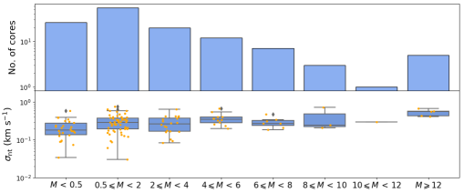
Figure 13: Nonthermal velocity dispersion derived from the emission of the deuterated species as function of the mass of the cores. In the upper panel is shown the number of cores per mass bin, and in the lower panel is shown a box plot with the mean and range of values of the nonthermal velocity dispersion per mass bin.

Figure 14: The core mass as a function of core radius. The blue solid line shows the linear regression to all the points in the plot, and the gray shadowed area shows the 1$\sigma$ confidence interval for the fit. The best fit gives a slope of 1.89 $\pm$ 0.11. The Spearman’s rank coefficient is 0.69 with the $p$-value of 1.0$\times 10^{-43}$.

References

- Astropy Collaboration et al. (2013) Astropy Collaboration, Robitaille, T. P., Tollerud, E. J., et al. 2013, A&A, 558, A33, doi: 10.1051/0004-6361/201322068
- Ayliffe et al. (2007) Ayliffe, B. A., Langdon, J. C., Cohl, H. S., & Bate, M. R. 2007, MNRAS, 374, 1198, doi: 10.1111/j.1365-2966.2006.11259.x
- Ballesteros-Paredes et al. (2011) Ballesteros-Paredes, J., Vázquez-Semadeni, E., Gazol, A., et al. 2011, MNRAS, 416, 1436, doi: 10.1111/j.1365-2966.2011.19141.x
- Barnes et al. (2021) Barnes, A. T., Henshaw, J. D., Fontani, F., et al. 2021, MNRAS, 503, 4601, doi: 10.1093/mnras/stab803
- Bergin & Tafalla (2007) Bergin, E. A., & Tafalla, M. 2007, ARA&A, 45, 339, doi: 10.1146/annurev.astro.45.071206.100404
- Bertoldi & McKee (1992) Bertoldi, F., & McKee, C. F. 1992, ApJ, 395, 140, doi: 10.1086/171638
- Beuther et al. (2002) Beuther, H., Schilke, P., Menten, K. M., et al. 2002, ApJ, 566, 945, doi: 10.1086/338334
- Beuther et al. (2018) Beuther, H., Soler, J. D., Vlemmings, W., et al. 2018, A&A, 614, A64, doi: 10.1051/0004-6361/201732378
- Billington et al. (2019) Billington, S. J., Urquhart, J. S., Figura, C., Eden, D. J., & Moore, T. J. T. 2019, MNRAS, 483, 3146, doi: 10.1093/mnras/sty3053
- Bonnell & Bate (2006) Bonnell, I. A., & Bate, M. R. 2006, MNRAS, 370, 488, doi: 10.1111/j.1365-2966.2006.10495.x
- Bonnell et al. (2001) Bonnell, I. A., Bate, M. R., Clarke, C. J., & Pringle, J. E. 2001, MNRAS, 323, 785, doi: 10.1046/j.1365-8711.2001.04270.x
- Bonnell et al. (2004) Bonnell, I. A., Vine, S. G., & Bate, M. R. 2004, MNRAS, 349, 735, doi: 10.1111/j.1365-2966.2004.07543.x
- Bontemps et al. (2010) Bontemps, S., Motte, F., Csengeri, T., & Schneider, N. 2010, A&A, 524, A18, doi: 10.1051/0004-6361/200913286
- Bovino et al. (2021) Bovino, S., Lupi, A., Giannetti, A., et al. 2021, A&A, 654, A34, doi: 10.1051/0004-6361/202141252
- Butler & Tan (2012) Butler, M. J., & Tan, J. C. 2012, ApJ, 754, 5, doi: 10.1088/0004-637X/754/1/5
- Caselli et al. (2002) Caselli, P., Benson, P. J., Myers, P. C., & Tafalla, M. 2002, ApJ, 572, 238, doi: 10.1086/340195
- Caselli et al. (1995) Caselli, P., Myers, P. C., & Thaddeus, P. 1995, ApJ, 455, L77+, doi: 10.1086/309805
- Chen et al. (2019) Chen, H. H.-H., Pineda, J. E., Goodman, A. A., et al. 2019, ApJ, 877, 93, doi: 10.3847/1538-4357/ab1a40
- Cohen (1988) Cohen, J. 1988, 1988 Statistical Power Analysis for the Behavioral Sciences (Hillsdale, NJ: L. Erlbaum Associates)
- Contreras et al. (2016) Contreras, Y., Garay, G., Rathborne, J. M., & Sanhueza, P. 2016, MNRAS, 456, 2041, doi: 10.1093/mnras/stv2796
- Contreras et al. (2017) Contreras, Y., Rathborne, J. M., Guzman, A., et al. 2017, MNRAS, 466, 340, doi: 10.1093/mnras/stw3110
- Contreras et al. (2013) Contreras, Y., Schuller, F., Urquhart, J. S., et al. 2013, A&A, 549, A45, doi: 10.1051/0004-6361/201220155
- Contreras et al. (2018) Contreras, Y., Sanhueza, P., Jackson, J. M., et al. 2018, ApJ, 861, 14, doi: 10.3847/1538-4357/aac2ec
- Csengeri et al. (2017) Csengeri, T., Bontemps, S., Wyrowski, F., et al. 2017, A&A, 600, L10, doi: 10.1051/0004-6361/201629754
- Cyganowski et al. (2017) Cyganowski, C. J., Brogan, C. L., Hunter, T. R., et al. 2017, MNRAS, 468, 3694, doi: 10.1093/mnras/stx043
- Dib et al. (2007) Dib, S., Kim, J., Vázquez-Semadeni, E., Burkert, A., & Shadmehri, M. 2007, ApJ, 661, 262, doi: 10.1086/513708
- Egan et al. (1998) Egan, M. P., Shipman, R. F., Price, S. D., et al. 1998, ApJ, 494, L199, doi: 10.1086/311198
- Elmegreen (2000) Elmegreen, B. G. 2000, ApJ, 530, 277, doi: 10.1086/308361
- Enoch et al. (2008) Enoch, M. L., Evans, II, N. J., Sargent, A. I., et al. 2008, ApJ, 684, 1240, doi: 10.1086/589963
- Fall & Frenk (1983) Fall, S. M., & Frenk, C. S. 1983, AJ, 88, 1626, doi: 10.1086/113452
- Federrath (2013) Federrath, C. 2013, MNRAS, 436, 1245, doi: 10.1093/mnras/stt1644
- Foster et al. (2011) Foster, J. B., Jackson, J. M., Barnes, P. J., et al. 2011, ApJS, 197, 25, doi: 10.1088/0067-0049/197/2/25
- Foster et al. (2013) Foster, J. B., Rathborne, J. M., Sanhueza, P., et al. 2013, PASA, 30, e038, doi: 10.1017/pasa.2013.18
- Friesen et al. (2009) Friesen, R. K., Di Francesco, J., Shirley, Y. L., & Myers, P. C. 2009, ApJ, 697, 1457, doi: 10.1088/0004-637X/697/2/1457
- Galtier & Banerjee (2011) Galtier, S., & Banerjee, S. 2011, Phys. Rev. Lett., 107, 134501, doi: 10.1103/PhysRevLett.107.134501
- Ginsburg & Mirocha (2011) Ginsburg, A., & Mirocha, J. 2011, PySpecKit: Python Spectroscopic Toolkit, Astrophysics Source Code Library, record ascl:1109.001. http://ascl.net/1109.001
- Guzmán et al. (2015) Guzmán, A. E., Sanhueza, P., Contreras, Y., et al. 2015, ApJ, 815, 130, doi: 10.1088/0004-637X/815/2/130
- Hartmann (2001) Hartmann, L. 2001, AJ, 121, 1030, doi: 10.1086/318770
- Henshaw et al. (2017) Henshaw, J. D., Jiménez-Serra, I., Longmore, S. N., et al. 2017, MNRAS, 464, L31, doi: 10.1093/mnrasl/slw154
- Heyer et al. (2009) Heyer, M., Krawczyk, C., Duval, J., & Jackson, J. M. 2009, ApJ, 699, 1092, doi: 10.1088/0004-637X/699/2/1092
- Heyer & Brunt (2004) Heyer, M. H., & Brunt, C. M. 2004, ApJ, 615, L45, doi: 10.1086/425978
- Hogerheijde et al. (1999) Hogerheijde, M. R., van Dishoeck, E. F., Salverda, J. M., & Blake, G. A. 1999, ApJ, 513, 350, doi: 10.1086/306844
- Hunter (2007) Hunter, J. D. 2007, Computing in Science Engineering, 9, 90
- Jackson et al. (2013) Jackson, J. M., Rathborne, J. M., Foster, J. B., et al. 2013, PASA, 30, 57, doi: 10.1017/pasa.2013.37
- Kauffmann et al. (2008) Kauffmann, J., Bertoldi, F., Bourke, T. L., Evans, N. J., I., & Lee, C. W. 2008, A&A, 487, 993, doi: 10.1051/0004-6361:200809481
- Kauffmann et al. (2013) Kauffmann, J., Pillai, T., & Goldsmith, P. F. 2013, ApJ, 779, 185, doi: 10.1088/0004-637X/779/2/185
- Kelly (2007) Kelly, B. C. 2007, ApJ, 665, 1489, doi: 10.1086/519947
- Kennicutt (1998) Kennicutt, Robert C., J. 1998, ARA&A, 36, 189, doi: 10.1146/annurev.astro.36.1.189
- Kirk et al. (2006) Kirk, H., Johnstone, D., & Di Francesco, J. 2006, ApJ, 646, 1009, doi: 10.1086/503193
- Kirk et al. (2010) Kirk, H., Pineda, J. E., Johnstone, D., & Goodman, A. 2010, ApJ, 723, 457, doi: 10.1088/0004-637X/723/1/457
- Kolmogorov (1941) Kolmogorov, A. 1941, Akademiia Nauk SSSR Doklady, 30, 301
- Kong et al. (2021) Kong, S., Arce, H. G., Shirley, Y., & Glasgow, C. 2021, ApJ, 912, 156, doi: 10.3847/1538-4357/abefe7
- Krumholz & Bonnell (2007) Krumholz, M. R., & Bonnell, I. A. 2007, ArXiv e-prints. https://arxiv.org/abs/0712.0828
- Krumholz et al. (2005) Krumholz, M. R., McKee, C. F., & Klein, R. I. 2005, Nature, 438, 332, doi: 10.1038/nature04280
- Larson (1981) Larson, R. B. 1981, MNRAS, 194, 809, doi: 10.1093/mnras/194.4.809
- Li et al. (2013) Li, D., Kauffmann, J., Zhang, Q., & Chen, W. 2013, ApJ, 768, L5, doi: 10.1088/2041-8205/768/1/L5
- Li et al. (2019) Li, S., Zhang, Q., Pillai, T., et al. 2019, ApJ, 886, 130, doi: 10.3847/1538-4357/ab464e
- Li et al. (2020a) Li, S., Zhang, Q., Liu, H. B., et al. 2020a, ApJ, 896, 110, doi: 10.3847/1538-4357/ab84f1
- Li et al. (2020b) Li, S., Sanhueza, P., Zhang, Q., et al. 2020b, ApJ, 903, 119, doi: 10.3847/1538-4357/abb81f
- Li et al. (2021) Li, S., Lu, X., Zhang, Q., et al. 2021, ApJ, 912, L7, doi: 10.3847/2041-8213/abf64f
- Li et al. (2022) Li, S., Sanhueza, P., Lu, X., et al. 2022, ApJ, 939, 102, doi: 10.3847/1538-4357/ac94d4
- Liu et al. (2020a) Liu, J., Zhang, Q., Qiu, K., et al. 2020a, ApJ, 895, 142, doi: 10.3847/1538-4357/ab9087
- Liu et al. (2020b) Liu, T., Evans, N. J., Kim, K.-T., et al. 2020b, MNRAS, 496, 2790, doi: 10.1093/mnras/staa1577
- Lu et al. (2014) Lu, X., Zhang, Q., Liu, H. B., Wang, J., & Gu, Q. 2014, ApJ, 790, 84, doi: 10.1088/0004-637X/790/2/84
- Lu et al. (2015) Lu, X., Zhang, Q., Wang, K., & Gu, Q. 2015, ApJ, 805, 171, doi: 10.1088/0004-637X/805/2/171
- Lu et al. (2018) Lu, X., Zhang, Q., Liu, H. B., et al. 2018, ApJ, 855, 9, doi: 10.3847/1538-4357/aaad11
- McKee (1999) McKee, C. F. 1999, in NATO Advanced Science Institutes (ASI) Series C, Vol. 540, NATO Advanced Science Institutes (ASI) Series C, ed. C. J. Lada & N. D. Kylafis, 29
- McKee & Ostriker (2007) McKee, C. F., & Ostriker, E. C. 2007, ARA&A, 45, 565, doi: 10.1146/annurev.astro.45.051806.110602
- McKee & Tan (2002) McKee, C. F., & Tan, J. C. 2002, Nature, 416, 59
- McMullin et al. (2007) McMullin, J. P., Waters, B., Schiebel, D., Young, W., & Golap, K. 2007, in Astronomical Society of the Pacific Conference Series, Vol. 376, Astronomical Data Analysis Software and Systems XVI, ed. R. A. Shaw, F. Hill, & D. J. Bell, 127
- Morii et al. (2021) Morii, K., Sanhueza, P., Nakamura, F., et al. 2021, ApJ, 923, 147, doi: 10.3847/1538-4357/ac2365
- Morii (2023) Morii, K. e. a. 2023, submitted to ApJ
- Myers & Benson (1983) Myers, P. C., & Benson, P. J. 1983, ApJ, 266, 309, doi: 10.1086/160780
- Nakamura & Li (2007) Nakamura, F., & Li, Z.-Y. 2007, ApJ, 662, 395, doi: 10.1086/517515
- Nony et al. (2023) Nony, T., Galvan-Madrid, R., Motte, F., et al. 2023, arXiv e-prints, arXiv:2301.07238, doi: 10.48550/arXiv.2301.07238
- Offner et al. (2008a) Offner, S. S. R., Klein, R. I., & McKee, C. F. 2008a, ApJ, 686, 1174, doi: 10.1086/590238
- Offner et al. (2008b) Offner, S. S. R., Krumholz, M. R., Klein, R. I., & McKee, C. F. 2008b, AJ, 136, 404, doi: 10.1088/0004-6256/136/1/404
- Ohashi et al. (2016) Ohashi, S., Sanhueza, P., Chen, H.-R. V., et al. 2016, ApJ, 833, 209, doi: 10.3847/1538-4357/833/2/209
- Padoan et al. (2001) Padoan, P., Juvela, M., Goodman, A. A., & Nordlund, Å. 2001, ApJ, 553, 227, doi: 10.1086/320636
- Padoan et al. (2020) Padoan, P., Pan, L., Juvela, M., Haugbølle, T., & Nordlund, Å. 2020, ApJ, 900, 82, doi: 10.3847/1538-4357/abaa47
- Palau et al. (2013) Palau, A., Fuente, A., Girart, J. M., et al. 2013, ApJ, 762, 120, doi: 10.1088/0004-637X/762/2/120
- Palau et al. (2014) Palau, A., Estalella, R., Girart, J. M., et al. 2014, ApJ, 785, 42, doi: 10.1088/0004-637X/785/1/42
- Pelkonen et al. (2021) Pelkonen, V. M., Padoan, P., Haugbølle, T., & Nordlund, Å. 2021, MNRAS, 504, 1219, doi: 10.1093/mnras/stab844
- Peretto et al. (2006) Peretto, N., André, P., & Belloche, A. 2006, A&A, 445, 979, doi: 10.1051/0004-6361:20053324
- Pillai et al. (2019) Pillai, T., Kauffmann, J., Zhang, Q., et al. 2019, A&A, 622, A54, doi: 10.1051/0004-6361/201732570
- Plume et al. (1997) Plume, R., Jaffe, D. T., Evans, Neal J., I., Martín-Pintado, J., & Gómez-González, J. 1997, ApJ, 476, 730, doi: 10.1086/303654
- Price-Whelan et al. (2018) Price-Whelan, A. M., Sip’ocz, B. M., G”unther, H. M., et al. 2018, aj, 156, 123, doi: 10.3847/1538-3881/aabc4f
- Rathborne et al. (2004) Rathborne, J. M., Simon, R., Jackson, J. M., & Shah, R. Y. 2004, in Astronomical Society of the Pacific Conference Series, Vol. 322, The Formation and Evolution of Massive Young Star Clusters, ed. H. J. G. L. M. Lamers, L. J. Smith, & A. Nota, 273–+
- Rathborne et al. (2016) Rathborne, J. M., Whitaker, J. S., Jackson, J. M., et al. 2016, PASA, 33, e030, doi: 10.1017/pasa.2016.23
- Redaelli et al. (2021) Redaelli, E., Bovino, S., Giannetti, A., et al. 2021, A&A, 650, A202, doi: 10.1051/0004-6361/202140694
- Redaelli et al. (2022) Redaelli, E., Bovino, S., Sanhueza, P., et al. 2022, arXiv e-prints, arXiv:2208.01675. https://arxiv.org/abs/2208.01675
- Rosolowsky et al. (2008) Rosolowsky, E. W., Pineda, J. E., Kauffmann, J., & Goodman, A. A. 2008, ApJ, 679, 1338, doi: 10.1086/587685
- Sabatini et al. (2019) Sabatini, G., Giannetti, A., Bovino, S., et al. 2019, MNRAS, 490, 4489, doi: 10.1093/mnras/stz2818
- Sabatini et al. (2022) Sabatini, G., Bovino, S., Sanhueza, P., et al. 2022, ApJ, 936, 80, doi: 10.3847/1538-4357/ac83aa
- Sakai et al. (2022) Sakai, T., Sanhueza, P., Furuya, K., et al. 2022, ApJ, 925, 144, doi: 10.3847/1538-4357/ac3d2e
- Sánchez-Monge et al. (2013) Sánchez-Monge, Á., Palau, A., Fontani, F., et al. 2013, MNRAS, 432, 3288, doi: 10.1093/mnras/stt679
- Sanhueza et al. (2010) Sanhueza, P., Garay, G., Bronfman, L., et al. 2010, ApJ, 715, 18, doi: 10.1088/0004-637X/715/1/18
- Sanhueza et al. (2012) Sanhueza, P., Jackson, J. M., Foster, J. B., et al. 2012, ApJ, 756, 60, doi: 10.1088/0004-637X/756/1/60
- Sanhueza et al. (2013) —. 2013, ApJ, 773, 123, doi: 10.1088/0004-637X/773/2/123
- Sanhueza et al. (2017) Sanhueza, P., Jackson, J. M., Zhang, Q., et al. 2017, ApJ, 841, 97, doi: 10.3847/1538-4357/aa6ff8
- Sanhueza et al. (2019) Sanhueza, P., Contreras, Y., Wu, B., et al. 2019, ApJ, 886, 102, doi: 10.3847/1538-4357/ab45e9
- Sanhueza et al. (2021) Sanhueza, P., Girart, J. M., Padovani, M., et al. 2021, ApJ, 915, L10, doi: 10.3847/2041-8213/ac081c
- Schuller et al. (2009) Schuller, F., Menten, K. M., Contreras, Y., et al. 2009, A&A, 504, 415, doi: 10.1051/0004-6361/200811568
- Shirley (2015) Shirley, Y. L. 2015, PASP, 127, 299, doi: 10.1086/680342
- Shirley et al. (2003) Shirley, Y. L., Evans, Neal J., I., Young, K. E., Knez, C., & Jaffe, D. T. 2003, ApJS, 149, 375, doi: 10.1086/379147
- Shu et al. (1987) Shu, F. H., Lizano, S., & Adams, F. C. 1987, in IAU Symposium, Vol. 115, Star Forming Regions, ed. M. Peimbert & J. Jugaku, 417–433
- Simon et al. (2006) Simon, R., Rathborne, J. M., Shah, R. Y., Jackson, J. M., & Chambers, E. T. 2006, ApJ, 653, 1325, doi: 10.1086/508915
- Singh et al. (2021) Singh, A., Matzner, C. D., Friesen, R. K., et al. 2021, ApJ, 922, 87, doi: 10.3847/1538-4357/ac20d2
- Smith et al. (2009) Smith, R. J., Longmore, S., & Bonnell, I. 2009, MNRAS, 400, 1775, doi: 10.1111/j.1365-2966.2009.15621.x
- Tafoya et al. (2021) Tafoya, D., Sanhueza, P., Zhang, Q., et al. 2021, ApJ, 913, 131, doi: 10.3847/1538-4357/abf5da
- Takemura et al. (2022) Takemura, H., Nakamura, F., Arce, H. G., et al. 2022, arXiv e-prints, arXiv:2211.10215. https://arxiv.org/abs/2211.10215
- Tan (2018) Tan, J. C. 2018, IAU Symposium, 332, 139, doi: 10.1017/S1743921317009784
- Teegavarapu (2019) Teegavarapu, R. S. 2019, in Trends and Changes in Hydroclimatic Variables, ed. R. Teegavarapu (Elsevier), 1–89, doi: https://doi.org/10.1016/B978-0-12-810985-4.00001-3
- Traficante et al. (2018a) Traficante, A., Fuller, G. A., Smith, R. J., et al. 2018a, MNRAS, 473, 4975, doi: 10.1093/mnras/stx2672
- Traficante et al. (2018b) Traficante, A., Lee, Y. N., Hennebelle, P., et al. 2018b, A&A, 619, L7, doi: 10.1051/0004-6361/201833513
- Traficante et al. (2018c) Traficante, A., Duarte-Cabral, A., Elia, D., et al. 2018c, MNRAS, 477, 2220, doi: 10.1093/mnras/sty798
- Tychoniec et al. (2021) Tychoniec, Ł., van Dishoeck, E. F., van’t Hoff, M. L. R., et al. 2021, A&A, 655, A65, doi: 10.1051/0004-6361/202140692
- Vázquez-Semadeni et al. (2009) Vázquez-Semadeni, E., Gómez, G. C., Jappsen, A.-K., Ballesteros-Paredes, J., & Klessen, R. S. 2009, ApJ, 707, 1023, doi: 10.1088/0004-637X/707/2/1023
- Vázquez-Semadeni et al. (2017) Vázquez-Semadeni, E., González-Samaniego, A., & Colín, P. 2017, MNRAS, 467, 1313, doi: 10.1093/mnras/stw3229
- Vázquez-Semadeni et al. (2019) Vázquez-Semadeni, E., Palau, A., Ballesteros-Paredes, J., Gómez, G. C., & Zamora-Avilés, M. 2019, MNRAS, 490, 3061, doi: 10.1093/mnras/stz2736
- Virtanen et al. (2020) Virtanen, P., Gommers, R., Oliphant, T. E., et al. 2020, Nature Methods, 17, 261, doi: 10.1038/s41592-019-0686-2
- Walsh et al. (2004) Walsh, A. J., Myers, P. C., & Burton, M. G. 2004, ApJ, 614, 194, doi: 10.1086/423425
- Wang et al. (2014) Wang, K., Zhang, Q., Testi, L., et al. 2014, MNRAS, 439, 3275, doi: 10.1093/mnras/stu127
- Ward-Thompson et al. (1994) Ward-Thompson, D., Scott, P. F., Hills, R. E., & Andre, P. 1994, MNRAS, 268, 276, doi: 10.1093/mnras/268.1.276
- Waskom (2021) Waskom, M. L. 2021, Journal of Open Source Software, 6, 3021, doi: 10.21105/joss.03021
- Whitaker et al. (2017) Whitaker, J. S., Jackson, J. M., Rathborne, J. M., et al. 2017, AJ, 154, 140, doi: 10.3847/1538-3881/aa86ad
- Zhang et al. (2015) Zhang, Q., Wang, K., Lu, X., & Jiménez-Serra, I. 2015, ApJ, 804, 141, doi: 10.1088/0004-637X/804/2/141
- Zhang et al. (2009) Zhang, Q., Wang, Y., Pillai, T., & Rathborne, J. 2009, ApJ, 696, 268, doi: 10.1088/0004-637X/696/1/268
- Zinnecker & Yorke (2007) Zinnecker, H., & Yorke, H. W. 2007, ARA&A, 45, 481, doi: 10.1146/annurev.astro.44.051905.092549