Decoupling Dynamic Monocular Videos for Dynamic View Synthesis

Abstract

The challenge of dynamic view synthesis from dynamic monocular videos, i.e., synthesizing novel views for free viewpoints given a monocular video of a dynamic scene captured by a moving camera, mainly lies in accurately modeling the dynamic objects of a scene using limited 2D frames, each with a varying timestamp and viewpoint. Existing methods usually require pre-processed 2D optical flow and depth maps by off-the-shelf methods to supervise the network, making them suffer from the inaccuracy of the pre-processed supervision and the ambiguity when lifting the 2D information to 3D. In this paper, we tackle this challenge in an unsupervised fashion. Specifically, we decouple the motion of the dynamic objects into object motion and camera motion, respectively regularized by proposed unsupervised surface consistency and patch-based multi-view constraints. The former enforces the 3D geometric surfaces of moving objects to be consistent over time, while the latter regularizes their appearances to be consistent across different viewpoints. Such a fine-grained motion formulation can alleviate the learning difficulty for the network, thus enabling it to produce not only novel views with higher quality but also more accurate scene flows and depth than existing methods requiring extra supervision. We will make the code publicly available at https://github.com/mengyou2/DecoulpingNeRF.

I Introduction

Novel view synthesis aims to generate new views of a scene from existing views or 3D models, allowing for immersive experiences in virtual/augmented reality [48, 8], robotics [26], and so on. In a more general scenario, dynamic view synthesis from dynamic monocular videos makes this field more prominent, in which given a monocular video of a scene containing moving objects captured by a moving camera, novel views at arbitrary viewpoints and timestamps will be synthesized to create visually stunning effects like the bullet-time effect, as demonstrated in Fig. 1. However, dynamic view synthesis is much more challenging due to the difficulty of accurately modeling dynamic objects in the scene using limited 2D frames, each with a varying timestamp and viewpoint.

[width=0.392loop, autoplay]4demo/umbrella/011

(a) Input Video

[width=0.268loop, autoplay]12demo/umbrella_crop/gao_188

(b) Gao et al. [13]

[width=0.268loop, autoplay]12demo/umbrella_crop/ours_188

(c) Ours

Figure 1: Given a monocular video of a dynamic scene captured by a moving camera, rendered novel views (zoomed in at dynamic part) at arbitrary viewpoints and any input timestep by state-of-the-art method Gao et al. [13] and Ours. Please use Adobe Acrobat to display these videos.

Recently, the advancements in deep learning have led to remarkable achievements in novel view synthesis. One of the most notable works in this field is the neural radiance field (NeRF) [29], which represents a scene using a continuous 5D volumetric function encoded by a multi-layer perceptron. Efforts are being made to expand the use of NeRF to dynamic view synthesis, such as learning a deformable warp field between different time frames and a canonical space [37, 43, 33] or a neural scene flow field (NSFF) between adjacent frames [21, 13, 10, 46]. Moreover, the NSFF is more capable of maintaining continuity across timestamps in real-world monocular videos than the deformable NeRF. However, previous methods usually require pre-processed 2D optical flow and depth maps by additional methods as supervision during network training, making them suffer from the following limitations. First, the inevitable local errors of the pre-processed supervision would harm the network and negatively affect the reconstruction quality, as demonstrated in Fig. 2. Second, using 2D maps to supervise 3D geometry would introduce ambiguity and result in inaccurate reconstructions. Finally, obtaining accurate pre-processed maps may be computationally expensive and time-consuming, making it inconvenient.

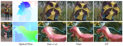
Figure 2: Visual illustration of the limitation of existing method Gao et al. [13]. The pre-processed 2D optical flow maps used for training networks contain severe errors, resulting in the corresponding parts of synthesized novel views being wrong.

In contrast to existing methods, we aim to tackle this challenge in an unsupervised manner, i.e., without using pre-processed information by off-the-shelf methods as supervision. Specifically, we propose to decouple the motion of dynamic objects in a scene into object motion and camera motion. Then, we propose two novel unsupervised regularization terms named surface consistency and multi-view consistency for modeling object motion and camera motion, respectively. The former ensures that the surface of moving objects remains geometrically consistent over time, while the latter ensures consistent appearance across different viewpoints. Such a fine-grained formulation of the motion of dynamic objects makes it easier for the network to model them. It is impressive that our unsupervised method even substantially improves state-of-the-art supervised methods. Besides, our method can output more accurate scene flow and depth. We believe our method will provide a promising baseline for dynamic view synthesis.

In summary, the main contributions of this paper are:

• fine-grained formulation of the motion of dynamic objects in a scene in a decoupling fashion;

• unsupervised surface consistency regularization for modeling object motion;

• unsupervised patch-based multi-view regularization for modeling camera motion; and

• current state-of-the-art performance of dynamic view synthesis and unsupervised scene flow and depth prediction.

The rest of this paper is orgarnized as follows. Section II briefly reviews related works. Section III reviews the general pipeline of NSFF-based novel view synthesis for dynamic videos. Section IV presents the proposed constraints for optimizing dynamic NeRF, followed by comprehensive experiments and analyses in Section V. Finally, Section VI concludes the paper and discusses some future directions for improving the proposed method.

II Related Work

II-A Novel View Synthesis for Static Scenes

View synthesis for static scenes is a long-standing problem in computer vision/graphics. Owing to the development of deep learning techniques, recent image-based rendering learns scene information with neural networks. Some methods [60, 5, 41, 32] adopt neural networks to estimate depth or appearance flow explicitly between viewpoints and use it to warp pixels from sources to the novel view. Many recent methods choose to learn 3D scene geometry with explicit scene representations which can be rendered to novel viewpoints. Some [54, 7, 16, 17, 36, 53, 15, 25] learn voxel-based grid from source images, representing objects as a 3D volume in the form of voxel occupancies. Another class of methods [59, 11, 28, 40, 23] use multiplane images (MPI) to represent the scene as a set of front-parallel planes at fixed depths, where each plane consists of an RGB image and an $\alpha$ map. Similar to MPI, LDI [38, 42, 45, 39, 9] keeps several depth and color values at every pixel and renders images by a back-to-front forward warping algorithm. Another explicit scene representation is the 3D point cloud. Some methods [50, 18, 3] project 2D images or features to the 3D point cloud space and generate novel views with a differentiable renderer.

More recent methods represent the scene as an NeRF [29] by learning a continuous volumetric scene function. Following methods extend NeRF in different aspects: reconstruction quality [57, 1], generalization [56, 47, 44, 6, 19, 4], unconstrained scene [27, 2], and so on.

II-B Novel View Synthesis for Dynamic Scenes

Novel view synthesis for dynamic scenes can be more challenging because multi-view geometry consistency does not apply to contents with motion. Recently, some image-based rendering methods [55, 24] have achieved impressive performance for dynamic view synthesis. Yoon et al. [55] proposed to blend depth-based warping with blending techniques for dynamic view synthesis. They used multi-view stereo for static parts and monocular depth estimation for dynamic parts, which are then blended for warping to the final result. Lin et al. [24] modeled a 3D scene using deep 3D mask volume representation based on MPI. The 3D scene is modeled as a background and an instantaneous MPI, added to a global MPI with predicted masks. However, these image-based rendering methods rely heavily on accurate depth estimation and are not flexible enough to render novel views from arbitrary viewpoints.

Recently, NeRF has achieved impressive performance in view synthesis tasks. Many methods have extended NeRF to address dynamic view synthesis. Some recent methods [49, 12, 35, 31] focus on specific domains, such as the face or human synthesis. Others focus on more general settings with video inputs capturing a global scene containing static and dynamic objects. There are three main ideas for extending NeRF: (1) incorporating time information or time-related latent codes into the input of NeRF [52, 20]; (2) learning a deformable NeRF [37, 43, 33]; and (3) learning 3D neural flow fields [21, 13, 10, 46].

Deformable NeRF splits the rendering process into two parts: a base NeRF encoding the canonical space and a warp field that maps the canonical NeRF into a deformed scene at another time. A multi-layer perceptron (MLP) is used to encode the frames at $t=0$, which is considered the canonical scene, while another MLP takes the points’ positions and time as input to produce the displacement between the point’s position in the current time and the canonical space. Pumarola et al. [37] applied this approach to dynamic synthetic objects. Tretschk et al. [43] further extended it to real dynamic scenes from monocular video by incorporating a rigidity prediction network. Park et al. introduced an elastic regularization of the deformation field to improve the regularization of NeRFs [33] and further handled topological changes by lifting NeRFs into a higher dimensional space [34]. Based on [34], Wu et al. [51] proposed to segment dynamic objects from the static background in a monocular video by using separate neural radiance fields to represent the moving objects and the static background in a self-supervised manner. However, the main challenge in deformable NeRF is handling large motions in the scene, as all frames are warped from the same canonical space, resulting in a lack of continuity throughout the sequence.

Neural scene flow fields model the dynamic scene as a time-variant continuous function of appearance, geometry, and 3D scene motion. Li et al. [21] proposed to estimate 3D motion by modeling scene flow as a dense 3D vector field. Given a 3D point and time, their methods output not only reflectance and opacity but also forward and backward scene flow. Gao et al. [13] adopted the same formulation and improved the reconstruction quality by further regulating the temporal consistency and rigidity of the neural scene flow. Du et al. [10] addressed a set of consistency losses regarding scene appearance, density, and motion to enforce consistency through the flow fields. Wang et al. [46] adopt a neural trajectory field to model the scene flow and parameterize the trajectory as a combination of sinusoidal bases, i.e., the discrete cosine transform. Li et al. [22] adopted a volumetric image-based rendering framework that addresses the challenges of blurry or inaccurate renderings in long videos for dynamic view synthesis by aggregating features from nearby views. Despite inheriting the simplicity and efficiency of NeRF, these methods often require additional regulations, particularly preprocessing data-driven terms, to function optimally.

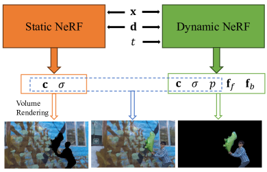
Figure 3: Our approach follows existing methods by utilizing two neural radiance fields: a static NeRF [29] for modeling the static background of a scene and an NSFF [21, 13] for modeling the dynamic objects and the scene flow. We train a Static NeRF model to reconstruct the scene background, excluding pixels marked as dynamic during training. We train a Dynamic NeRF that takes (x, d) and t as input for modeling dynamic objects. This allows the Dynamic NeRF to predict color c, density $\sigma$, 3D scene flow $\textbf{f}_{f},\textbf{f}_{b}$, and blending weight $p$. The blending weight $p$ enables the composition of static and dynamic NeRF components.

III Preliminary

Let $\mathcal{I}:=\left\{\mathbf{I}_{n}\in\mathbb{R}^{H\times W}\right\}_{n=1}^{N}$ denote a dynamic monocular video, consisting of $N$ frames, each of dimensions $H\times W$. Each frame $\mathbf{I}_{n}$ associates with a timestamp $t_{n}$ and a camera pose $\mathbf{p}_{n}$. Given $\mathcal{I}$ and $\{t_{n},\mathbf{p}_{n}\}_{n=1}^{N}$, dynamic view synthesis aims at synthesizing novel views at arbitrarily given viewpoints and timestamps. This task is challenging because the 3D geometry of dynamic objects in the scene varies across different timestamps, while the monocular video only provides a single 2D observation of them at each timestamp. Existing methods [21, 13] use two neural radiance fields: a static NeRF [29] to model the static background of a scene, and an NSFF [21, 13] to model the dynamic objects and the scene flow.

Static NeRF adopts the plain NeRF to model the static background of a scene. Specifically, for a 3D point $\mathbf{x}\in\mathbb{R}^{3}$ sampled on a ray $\mathbf{r}(s)=\mathbf{o}+s\mathbf{d}$ with the origin $\mathbf{o}\in\mathbb{R}^{3}$ and the normalized viewing direction $\mathbf{d}\in\mathbb{R}^{3}$, the static NeRF uses an MLP $\texttt{MLP}_{s}(\cdot)$ to map directional $\mathbf{x}$ to an RGB color $\mathbf{c}_{s}$ and a density $\sigma_{s}$:

$$(\mathbf{c}_{s},\sigma_{s})=\texttt{MLP}_{s}(\mathbf{x},\mathbf{d}).$$ (1)

The static NeRF is trained by minimizing

$$\mathcal{L}_{static}=\sum_{\mathbf{r}\in\mathcal{R}}\|(\mathbf{\widehat{C}}_{s}(\mathbf{r})-\mathbf{C}(\mathbf{r}))(1-M(\mathbf{r}))\|_{2}^{2},$$ (2)

where $\mathcal{R}$ is the set of rays in each batch, $\mathbf{\widehat{C}}_{s}(\mathbf{r})$ computed with the volume rendering integral is the rendered color of the pixel the ray r passes through, $\mathbf{C}(\mathbf{r})$ is the ground truth color value, and $M$ is the preprocessed mask indicating the dynamic part.

NSFF. Taking $(\mathbf{x},~{}\mathbf{d},~{}t)$ as input, where $t$ is the timestamp of the frame, NSFF outputs the forward 3D scene flow $\mathbf{f}_{f}$ from $t$ to $t+1$, the backward 3D scene flow $\mathbf{f}_{b}$ from $t$ to $t-1$, and a probability value $p$ indicating the dynamic part, in addition to the volume density and view-dependent emitted radiance:

$$(\mathbf{c}^{t}_{d},\sigma^{t}_{d},\mathbf{f}_{f},\mathbf{f}_{b},p)=\texttt{MLP}_{d}(\mathbf{x},\mathbf{d},t),$$ (3)

where $\texttt{MLP}_{d}(\cdot)$ is the learnable MLP.

Thus, time neighboring points can be computed easily by $\mathbf{x}+\mathbf{f}_{f}$ and $\mathbf{x}+\mathbf{f}_{b}$. By querying these points, the corresponding color, density, and forward/backward flow can be predicted by the same MLP:

$$\begin{split}\begin{aligned} (\mathbf{c}_{d}^{t+1},\sigma_{d}^{t+1},\mathbf{f}_{ff},\mathbf{f}_{fb})=\texttt{MLP}_{d}(\mathbf{x}+\mathbf{f}_{f},\mathbf{d},t+1),\\ (\mathbf{c}_{d}^{t-1},\sigma_{d}^{t-1},\mathbf{f}_{bf},\mathbf{f}_{bb})=\texttt{MLP}_{d}(\mathbf{x}+\mathbf{f}_{b},\mathbf{d},t-1).\end{aligned}\end{split}$$ (4)

The rendering color $\mathbf{\widehat{C}}^{\overline{t}}_{d}$ of the ray $\mathbf{r}$ in the consequent three timestamps $\overline{t}\in\left\{t-1,t,t+1\right\}$ can be computed with the volume rendering integral. NSFF can be trained with minimizing

$$\mathcal{L}_{dynamic}=\sum_{\overline{t}\in\left\{t-1,t,t+1\right\}}\sum_{\mathbf{r}\in\mathcal{R}}\|\mathbf{\widehat{C}}_{d}^{\overline{t}}(\mathbf{r})-\mathbf{C}(\mathbf{r})\|_{2}^{2}.$$ (5)

At the same time, the scene flow $\mathbf{f}_{f}$ and $\mathbf{f}_{b}$ are supervised with the pre-processed 2D optical flow by an off-the-shelf method during training. Specifically, each 3D position corresponding to 2D pixel at time $t$ is warped to the reference frame via $\mathbf{f}_{f}$ and $\mathbf{f}_{b}$ and then projected onto the reference camera to generate 2D optical flow, which is enforced to approach the pre-processed 2D optical flow by a pre-trained network. Also, the expected termination depth along each ray and the predicted dynamic probability $p$ are supervised with the pre-processed depth and mask by off-the-shelf methods, respectively.

In addition, the NSFF model is also regularized by the following constraints. $\|\mathbf{f}_{f}\|_{1}$ and $\|\mathbf{f}_{b}\|_{1}$ are minimized to promote the predicted scene flow to be temporally smooth and slow, and $\|\mathbf{f}_{f}+\mathbf{f}_{fb}\|_{2}$ and $\|\mathbf{f}_{b}+\mathbf{f}_{bf}\|_{2}$ are minimized to promote the scene flow to be consistent. The depth maps from the static NeRF are used to restrict those from NSFF. To ensure that only a few samples representing the dynamic objects dominate the rendering of the NSFF, the entropy of the rendering weights $T_{d}$ along each ray is minimized.

Finally, the static NeRF and NSFF are fused by leading the predicted dynamic probability value $p$ into the rendering equation to produce a composite color:

$$\begin{split}\mathbf{\widehat{C}}_{f}(r)=\int_{s_{n}}^{s_{f}}T_{f}(s)\big{(}(1-p)\sigma_{s}(\mathbf{r}(s))\mathbf{c}_{s}(\mathbf{r}(s),\mathbf{d})\\ +p\sigma_{d}(\mathbf{r}(s))\mathbf{c}_{d}(\mathbf{r}(s),\mathbf{d})\big{)}dt,\end{split}$$ (6)

where

$$T_{f}=\texttt{Exp}(-{\int_{s_{n}}^{s}}\big{(}(1-p)\sigma_{s}(\mathbf{r}(q))\big{)}\big{(}p\sigma_{d}(\mathbf{r}(q))\big{)}dq),$$ (7)

and $s_{n}$, and $s_{f}$ are the near and far bounds of the scene, respectively. Also, $\widehat{\mathbf{C}}_{f}$ is supervised with the ground-truth, i.e.,

$$\mathcal{L}_{full}=\sum_{\mathbf{r}\in\mathcal{R}}\|\mathbf{\widehat{C}}_{f}(\mathbf{r})-\mathbf{C}(\mathbf{r})\|_{2}^{2}.$$ (8)

IV Proposed Method

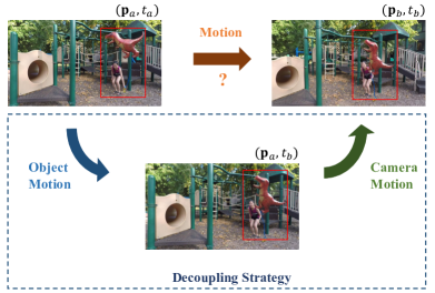
Figure 4: Given two successive frames of a dynamic monocular video with their camera poses and timestamps being $(\mathbf{p}_{a},~{}t_{a})$ and $(\mathbf{p}_{b},~{}t_{b})$. Directly modeling the motion of the dynamic objects (highlighted in red frames) between them can be challenging. Here, we propose to decouple the motion between them into two types: (1) the motion caused by the object movement; and (2) the motion caused by the camera movement.

Motivation. As aforementioned, to tackle the challenge of modeling the dynamic objects of a scene, existing dynamic view synthesis methods adopt pre-processed 2D optical flow and depth maps by off-the-shelf methods to supervise the NSFF explicitly. However, such a manner suffers from the following drawbacks. The pre-processed maps inevitably contain inaccurate regions, which would be harmful to the network during training, and thus compromise the quality of synthesized views, as demonstrated in Fig. 2. Moreover, the ambiguity exists when using the pre-processed 2D information to supervise the 3D geometry of the scene, as the same 2D pixels can result from various density and radiance distributions on the ray due to the rendering integral, leading to an unlimited number of possible explanations. Finally, obtaining accurate pre-processed maps may be computationally expensive and time-consuming, making it inconvenient.

Our Solution. Unlike existing methods, we tackle this challenging problem in an unsupervised manner. Generally, as shown in Fig. 4, we propose to decouple the motion of dynamic objects between two successive frames of a monocular video, such that the transition/flow from $\mathbf{I}_{a}$ at $(\mathbf{p}_{a},t_{a})$ to $\mathbf{I}_{b}$ at $(\mathbf{p}_{b},t_{b})$ can be modeled by first transforming the timestamp only with object motion involved, and then transforming the pose coordinate only with camera motion involved. Such a decoupling process can produce a fine-grained formulation of the motion of dynamic objects to alleviate the network’s difficulty in learning their complex 3D motion from extremely limited 2D observations. In accordance with our decoupling modeling approach, we propose two unsupervised regularization terms to enforce the network to learn under this paradigm. These terms are the surface consistency constraint (Sec. IV-A), which addresses temporal changes, and the patch-based multi-view constraint (Sec. IV-B), which addresses camera changes. Note that our method is built upon Gao et al. [13] without using pre-processed optical flow and depth as supervision. In the following, we will detail the two proposed constraints.

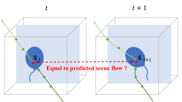
Figure 5: Illustration of the surface consistency constraint. Under the NeRF scheme, at timestamp $t$, we sample points (green points) on a ray and predict their density values to compute the weights they contribute to the rendering. The intersection point $\hat{\mathbf{x}}_{t}$ between the surface and the ray can be calculated by a weighted averaging of the coordinates of the sampled points. With NSFF, we can predict a 3D scene flow for each of the sampled points and warp them to the next timestamp $t+1$. Also, we can calculate the intersection point $\hat{\mathbf{x}}_{t+1}$ between the warped ray and the surface by a weighted averaging of the coordinates of the warped points. Our surface consistency constraint requires the difference between $\hat{\mathbf{x}}_{t}$ and $\hat{\mathbf{x}}_{t+1}$ should equal the scene flow predicted for the intersection point at $t$ by NSFF.

IV-A Surface Consistency Constraint

Assuming that the 3D geometric surface of a moving object is dynamically consistent throughout the video, we propose the surface consistency constraint to regularize the object motion among different timestamps, That is, the surface in the current timestamp should be correctly mapped to scene surfaces in its neighboring timestamps using the NSFF. To be more specific, we ensure that the predicted flow for a point on the scene surface at time $t$ accurately maps that point to the surface at time $t+1$.

Specifically, as illustrated in Fig. 5, for the ray $\mathbf{r}$ at time $t$, we sample $K$ points $\left\{\mathbf{x}_{i}\right\}_{i=1}^{K}$ for NeRF optimization and predict their corresponding density value, denoted as $\{\sigma_{d,i}^{t}\}_{i=1}^{K}$. For each point, we calculate the weight indicating its contribution to the rendering as

$$w_{d,i}^{t}=T_{d}\sigma_{d,i}^{t},$$ (9)

where

$$T_{d,i}=\texttt{Exp}(-{\int_{s_{n}}^{s_{i}}}\sigma_{d}^{t}(\mathbf{r}(q))dq),$$ (10)

where $s_{i}$ is the distance between $\mathbf{x}_{i}$ and $\mathbf{o}$. Also, for $\mathbf{r}$ at time $t$, we predict its intersection point with the scene surface, denoted as $\widehat{\mathbf{x}}_{t}$, by a weighted average of the coordinates of the sampled points over $\mathbf{r}$:

$$\widehat{\mathbf{x}}_{t}=\sum_{i=1}^{K}w_{d,i}^{t}\cdot\mathbf{x}_{i}.$$ (11)

With the scene flow $\mathbf{f}_{f}$ by NSFF (i.e., Eq. (3)), we can warp ray $\mathbf{r}$ to the next timestamp $t+1$:

$$\widetilde{\mathbf{x}}_{i}=\mathbf{x}_{i}+\mathbf{f}_{f}(\mathbf{x}_{i}),$$ (12)

where $\mathbf{f}_{f}(\mathbf{x}_{i})$ refers to the scene flow for $\mathbf{x}_{i}$, and $\widetilde{\mathbf{x}}_{i}$ is the warped point of $\mathbf{x}_{i}$. Note that the scene flow $\mathbf{f}_{f}$ is only an output of NSFF and NOT supervised during training in our framework. Similar to the above process, for $\widetilde{\mathbf{x}}_{i}$, we can also predict the corresponding weight $w_{d,i}^{t+1}$ and the intersection point of the warped ray with the scene surface at $t+1$, denoted as $\widehat{\mathbf{x}}_{t+1}$:

$$\widehat{\mathbf{x}}_{t+1}=\sum_{i=1}^{K}w_{d,i}^{t+1}\cdot\widetilde{\mathbf{x}}_{i}.$$ (13)

Based on the fact that the scene flow-induced surface should be consistent with the predicted surface, we propose a point-to-point loss by enforcing the warped intersection point of $\widehat{\mathbf{x}}_{t}$ by the flow, denoted as $\widehat{\mathbf{x}}_{t}+\mathbf{f}_{f}(\widehat{\mathbf{x}}_{t})$, to coincide with $\widehat{\mathbf{x}}_{t+1}$, i.e.,

$$\mathcal{L}_{surface}=\sum_{\mathbf{r}\in\mathcal{R}}\left\|(\widehat{\mathbf{x}}_{t}+\mathbf{f}_{f}(\widehat{\mathbf{x}}_{t}))-\widehat{\mathbf{x}}_{t+1}\right\|_{1},$$ (14)

where $\left\|\cdot\right\|_{1}$ is the $\ell_{1}$-norm of a vector. We also apply this loss to the previous timestamp $t-1$.

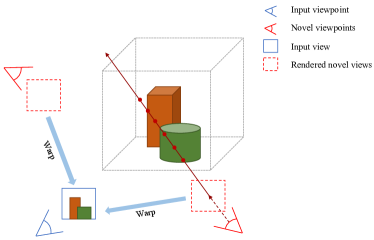
Figure 6: Illustration of the patch-based multi-view constraint. Under a certain timestamp, we enforce the multi-view consistency between the single input view and unknown novel viewpoints. We can synthesize a well-quality RGB-D image at the input viewpoint (blue viewpoint) owing to the capacity of NeRF. We then randomly sample novel viewpoints (red viewpoints) and render novel views in patch-wise for efficiency. The rendered novel view is warped to the input viewpoint using the rendered depth map for the input viewpoint. We compute the photometric reconstruction loss between the warped and rendered patches of the input view for efficiency.

IV-B Patch-based Multi-view Constraint

Here we propose the multi-view constraint to ensure consistency between the single input view and synthesized novel views at the same timestamp, enhancing the ability of the network to handle various camera movements. Moreover, we implement this constraint patch-wise for efficiency.

Taking time $t_{m}$ ($m=1,~{}2,~{}\cdots,~{}N$) as an example. Specifically, as shown in Fig. 6, at $t_{m}$, we have a single input view $\mathbf{I}_{m}$ associated with its camera pose $\mathbf{p}_{m}$ available. Owing to the powerful capability of NeRF, we can synthesize a well-quality patch $\mathbf{I}_{s}^{p}$ and derive a reasonable depth map $\mathbf{D}_{s}^{p}$ for this known viewpoint. We assume that this RGB-D map accurately represents the appearance and geometry of the scene and can thus serve as supervision for the synthesized novel views. To train a robust model, we randomly select a viewpoint $\mathbf{p}_{r}$ as the object of supervision and render a new patch $\mathbf{I}_{r}^{p}$. With $\mathbf{D}_{s}^{p}$, we inversely warp $\mathbf{I}_{r}^{p}$ to the viewpoint $\mathbf{p}_{m}$, written as

$$\widetilde{\mathbf{I}}_{s}^{p}=\mathcal{W}(\mathbf{I}_{r}^{p},~{}\mathbf{D}_{s}^{p},~{}\mathbf{p}_{r},~{}\mathbf{p}_{m}),$$ (15)

where $\mathcal{W}(\cdot)$ denotes the inverse warping operation. Finally, we formulate the patch-based multi-view constraint as

$$\mathcal{L}_{patch}=\|\mathbf{M_{w}}\odot(\mathbf{I}_{s}^{p}-\widetilde{\mathbf{I}}_{s}^{p})\|_{1},$$ (16)

where $\mathbf{M_{w}}$ is the induced mask by the inverse warping operation, and $\odot$ denotes the Hadamard product.

TABLE I: Pre-processed optical flow maps and depth maps supervision used in different methods. “$\checkmark$” (resp. “$\times$”) represents the corresponding term is used (resp. unused).

	Optical flow maps	Depth maps
Yoon et al. [55]	$\checkmark$	$\checkmark$
Tretschk et al. [43]	$\times$	$\times$
Li et al. [21]	$\checkmark$	$\checkmark$
Gao et al. [13]	$\checkmark$	$\checkmark$
Ours	$\times$	$\times$

TABLE II: Quantitative comparison of different methods on the Dynamic Scene Dataset. $\uparrow$ (resp. $\downarrow$) means the larger (resp. smaller), the better. The best and second best results are highlighted in bold and underline, respectively.

PSNR$\uparrow$ / SSIM$\uparrow$ / LPIPS$\downarrow$	Balloon1	Balloon2	Jumping	Playground
NeRF[29]	19.82 / 0.699 / 0.287	24.37 / 0.815 / 0.180	20.99 / 0.687 / 0.418	21.07 / 0.768 / 0.240
NeRF-t	18.54 / 0.443 / 0.419	20.69 / 0.570 / 0.349	18.04 / 0.465 / 0.535	14.68 / 0.230 / 0.534
Yoon et al. [55]	18.74 / 0.606 / 0.248	19.88 / 0.416 / 0.288	20.15 / 0.616 / 0.250	15.08 / 0.249 / 0.309
Tretschk et al. [43]	17.39 / 0.363 / 0.496	22.41 / 0.708 / 0.319	20.09 / 0.630 / 0.416	15.06 / 0.240 / 0.458
Li et al. [21]	21.96 / 0.702 / 0.288	24.27 / 0.740 / 0.288	24.65 / 0.813 / 0.227	21.22 / 0.717 / 0.268
Gao et al. [13]	22.36 / 0.773 / 0.173	27.06 / 0.864 / 0.117	24.68 / 0.843 / 0.151	24.15 / 0.858 / 0.148
Ours	22.49 / 0.773 / 0.186	27.34 / 0.870 / 0.120	24.09 / 0.823 / 0.162	24.62 / 0.864 / 0.147
PSNR$\uparrow$ / SSIM$\uparrow$ / LPIPS$\downarrow$	Skating	Truck	Umbrella	Average
NeRF [29]	23.67 / 0.781 / 0.418	22.73 / 0.747 / 0.334	21.29 / 0.546 / 0.457	21.99 / 0.720 / 0.333
NeRF-t	20.32 / 0.504 / 0.558	18.33 / 0.4380 / 0.524	17.69 / 0.267 / 0.667	18.33 / 0.417 / 0.512
Yoon et al. [55]	21.75 / 0.561 / 0.262	21.53 / 0.623 / 0.172	20.35 / 0.543 / 0.243	19.64 / 0.517 / 0.253
Tretschk et al. [43]	23.95 / 0.732 / 0.343	19.33 / 0.462 / 0.546	19.63 / 0.380 / 0.480	19.69 / 0.502 / 0.437
Li et al. [21]	29.29 / 0.888 / 0.190	25.96 / 0.774 / 0.249	22.97 / 0.659 / 0.319	24.33 / 0.756 / 0.261
Gao et al. [13]	32.66 / 0.951 / 0.080	28.56 / 0.872 / 0.149	23.26 / 0.720 / 0.193	26.10 / 0.840 / 0.144
Ours	33.66 / 0.955 / 0.084	28.63 / 0.871 / 0.172	23.71 / 0.726 / 0.186	26.36 / 0.840 / 0.151

TABLE III: Quantitative comparison of different methods on the dynamic part of a scene. $\uparrow$ (resp. $\downarrow$) means the larger (resp. smaller), the better. The best and second best results are highlighted in bold and underline, respectively.

PSNR$\uparrow$ / SSIM$\uparrow$ / LPIPS$\downarrow$	Balloon1	Balloon2	Jumping	Playground
NeRF[29]	17.06 / 0.562 / 0.395	19.74 / 0.631 / 0.273	16.95 / 0.471 / 0.480	16.62 / 0.618 / 0.337
NeRF-t	17.01 / 0.375 / 0.447	17.47 / 0.316 / 0.469	14.08 / 0.248 / 0.578	13.99 / 0.147 / 0.571
Yoon et al. [55]	17.46 / 0.505 / 0.318	18.59 / 0.332 / 0.272	17.17 / 0.466 / 0.289	13.86 / 0.188 / 0.402
Tretschk et al. [43]	16.69 / 0.341 / 0.531	18.69 / 0.531 / 0.425	15.88 / 0.357 / 0.514	13.83 / 0.136 / 0.573
Li et al. [21]	19.73 / 0.609 / 0.334	21.57 / 0.590 / 0.351	20.61 / 0.668 / 0.286	20.09 / 0.697 / 0.275
Gao et al. [13]	19.49 / 0.647 / 0.251	22.93 / 0.738 / 0.157	19.95 / 0.669 / 0.237	19.76 / 0.726 / 0.221
Ours	19.80 / 0.653 / 0.265	23.45 / 0.763 / 0.175	19.46 / 0.629 / 0.262	20.63 / 0.753 / 0.195
PSNR$\uparrow$ / SSIM$\uparrow$ / LPIPS$\downarrow$	Skating	Truck	Umbrella	Average
NeRF [29]	14.44 / 0.406 / 0.563	15.40 / 0.370 / 0.471	13.96 / 0.290 / 0.624	16.31 / 0.478 / 0.449
NeRF-t	14.27 / 0.284 / 0.648	15.58 / 0.278 / 0.481	14.29 / 0.188 / 0.720	15.24 / 0.262 / 0.559
Yoon et al. [55]	15.00 / 0.251 / 0.358	19.32 / 0.523 / 0.207	14.50 / 0.326 / 0.425	16.56 / 0.370 / 0.324
Tretschk et al. [43]	14.37 / 0.324 / 0.561	16.95 / 0.304 / 0.540	14.04 / 0.208 / 0.647	15.78 / 0.315 / 0.542
Li et al. [21]	21.65 / 0.651 / 0.271	23.38 / 0.689 / 0.213	15.90 / 0.401 / 0.463	20.42 / 0.615 / 0.313
Gao et al. [13]	21.68 / 0.680 / 0.201	23.21 / 0.706 / 0.121	15.79 / 0.428 / 0.361	20.40 / 0.656 / 0.221
Ours	23.31 / 0.771 / 0.208	23.65 / 0.714 / 0.190	16.52 / 0.470 / 0.320	20.97 / 0.679 / 0.231

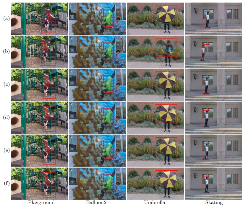
Figure 7: Visual comparison of different methods on Dynamic Scene Dataset. (a) Yoon et al. [55], (b) Tretschk et al. [43], (c) Li et al. [21], (d) Gao et al. [13], (e) Ours, (f) Ground Truth. Dynamic regions are highlighted in the red rectangular.

Remark. The concept of utilizing multi-view consistency to enhance NeRF in handling sparse views is similar between our method and RegNeRF [30]. However, the specific idea of the patch-based multi-view constraint in our method differs significantly from that of RegNeRF [30] In our approach, we focus on using a single input view to supervise other viewpoints within a specific timestamp. We achieve this by warping unknown viewpoints, represented as patches, to align with the input view and then applying RGB consistency loss for supervision. On the other hand, RegNeRF samples unobserved viewpoints in 3D space and directly renders a patch from the selected viewpoint. They utilize depth smoothness loss and RGB log-likelihood loss for their training process. While both methods share the idea of multi-view consistency, our patch-based approach involves a warping process that distinguishes it from RegNeRF’s methodology, which primarily relies on depth smoothness and RGB log-likelihoods without warping.

V Experiments

V-A Experiment Settings

Dataset. We conducted extensive experiments on the NVIDIA Dynamic Scene Dataset [55]. For each scene, the dataset provides 12 sequences captured by 12 fixed cameras. The scene contains a static background and a moving object in the foreground. We followed the setting of training/testing data and pre-processing protocol of Gao et al. [13]. The input video is obtained by selecting the $i$-th view at time $t_{i}$. In this way, each input view has a different viewpoint and timestamp from others. The evaluation set is determined by fixing the camera to the first view and changing timestamps.

Implementation details. Our approach follows NeRF to use positional encoding for input coordinates. For NSFF, we add an extra positional encoding of time. We sample 64 points along each ray for both training and testing. We first train the static NeRF and then fix its network parameters when training the NSFF. Training a full model takes approximately one day per scene using one NVIDIA GeForce RTX 3090 GPU, and rendering a single frame takes roughly 3 seconds.

V-B Comparison with State-of-the-Art Methods

We compared our method with six methods: NeRF [29], NeRF-t (a straightforward extension of NeRF by incorporating the time dimension into the input coordinate), an image-based rendering method Yoon et al. [55], a deformable NeRF-based method Tretschk et al. [43], and two NSFF-based methods Li et al. [21] and Gao et al. [13]. We also summarize whether they use pre-processed optical flow or depth as supervision in Table I.

Quantitative comparisons. Table II lists the PSNR, SSIM, and LPIPS [58] values of different methods on each of the scenes in the Dynamic Scene Dataset. From Table II, it can be observed that

• Ours outperforms all comparison methods in terms of the average PSNR for 7 scenes and achieves the highest PSNR on 6 out of 7 scenes. Regarding SSIM and LPIPS, Ours performs significantly better than other methods, except Gao et al. [13] that utilizes pre-processed depth and optical flow maps predicted by well-trained state-of-the-art models, providing the network with more information and indicating the movement of objects at a pixel level. Although our model can regularize the motion part using unsupervised losses, this is much less straight and forceful compared to these explicit supervisions, which may result in blurry moving objects, thus limiting LPIPS;

• the superiority of Ours in handling dynamic scenes is more evident in scenes with significant motion, such as Skating, Playground, and Umbrella, where it improves the reconstruction quality of the second best method by more than 0.5 dB;

• regarding the scene named Jumping, Ours does not perform as well as Li et al. [21] and Gao et al. [13]. The scene contains dynamic content primarily consisting of people jumping, which involves intricate non-rigid deformations. Our surface consistency constraint becomes invalid when dealing with non-rigid deformations.
  

Note that in our framework, we adopt the same model as Gao et al. [13] and Li et al. [21] to synthesize the static background of a scene, and the proposed two constraints are only imposed on NSFF. To directly demonstrate the advantages of our constraints, we present the quantitative results of different methods only on the dynamic part of a scene in Table III, where it can be seen that the superiority of our method over other methods is more significant.

Qualitative comparisons. In Fig. 7, we compared the visual results of different methods on four scenes from the Dynamic Scene Dataset. Our method produces better reconstruction results for dynamic objects compared to all other compared methods under the same experimental configuration. Yoon et al. [55] shows slight bias in the orientation and position of dynamic objects in complex scenes. Trestchk et al. [43] struggles to guarantee the integrity of synthetic objects in complex scenes and fails to model motion correctly for scenes with significant movements. While Li et al. [21] can accurately model dynamic objects, it produces blurry and less detailed results. Gao et al. [13] fails to handle thin edges, such as the rope of the balloon and the strip of the umbrella, and generates blurry or artifact-laden regions containing large motions. We also refer the reviewers to the associated video demo.

TABLE IV: Quantitative results of the ablative study on the two proposed constraints.

	PSNR$\uparrow$	SSIM$\uparrow$	LPIPS$\downarrow$
Baseline	24.81	0.822	0.161
Baseline+$\mathcal{L}_{surface}$	25.95	0.838	0.154
Baseline+$\mathcal{L}_{patch}$	25.35	0.829	0.151
Full (Baseline+$\mathcal{L}_{surface}$+$\mathcal{L}_{patch}$)	26.36	0.840	0.151

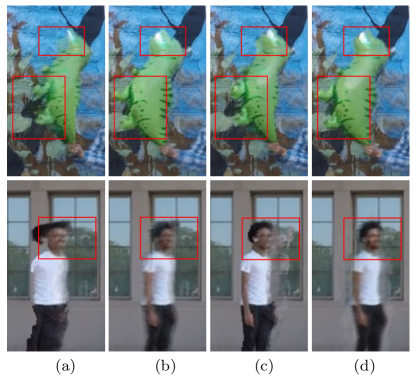
Figure 8: Visual comparison of ablations of (a) Baseline, (b) Baseline+$\mathcal{L}_{surface}$, (c) Baseline+$\mathcal{L}_{patch}$, (d) Full model (Baseline+$\mathcal{L}_{surface}$+$\mathcal{L}_{patch}$).

V-C Ablation Study

We conducted ablation studies to understand the two proposed regularization terms better. We excluded these two terms from the complete framework to construct the baseline while keeping other regularization terms unchanged. Note that this baseline is actually the approach of Gao et al. [13] without flow/depth supervision. To isolate the effects of the two key regularization terms on the dynamic objects, we used the same static model for all experiments in the ablation study, as we separated the static part and the dynamic part of scenes in our approach.

Table IV lists the quantitative results, where it can be seen that each of the two terms can significantly improve the baseline, and the reconstruction quality is further improved largely when simultaneously using the two terms. Besides, as visualized in Fig. 8, the baseline model cannot predict the correct trajectory for dynamic objects, leading to distortions, artifacts, and blurs. The surface consistency constraint enables us to map the dynamic motions accurately and ensures object geometry consistency, while the patch-based multi-view consistency constraint produces sharper, clearer reconstructions with more details. The full model can accurately model dynamic movements and produce clear results, even for videos with large object motion.

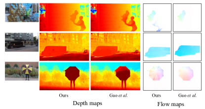
Figure 9: Visual comparison of rendered depth maps and 2D optical flow maps of our method and Gao et al. [13]. We masked the optical flow maps using the estimated dynamic mask.

TABLE V: Comparison of the predicted scene flows by Gao et al. [13] and Ours using PCK-T. $\uparrow$ means the larger, the better.

PCK-T$\uparrow$	Balloon1	Balloon2	Jumping	Playground
Gao et al. [13]	0.819	0.886	0.955	0.962
Ours	0.673	0.909	0.946	0.970
PCK-T$\uparrow$	Skating	Truck	Umbrella	-
Gao et al. [13]	1.00	0.936	0.744	-
Ours	1.00	0.978	0.767	-

V-D Comparison of Flow and Depth Estimation

Our method can predict the depth and flow maps of novel views in an unsupervised manner. Note that the 2D optical flow is obtained by projecting the predicted 3D scene flow to the camera space. As shown in Fig. 9, despite some noise, our results exhibit strong structure awareness and can smoothly handle slight depth/flow changes across different parts of the same object. The flow and depth maps of novel views by our method are comparable to or even more accurate than those by Gao et al. [13] that adopts pre-processed depth and flow maps as supervision, which is credited to our fine-grained formulation.

To quantitatively evaluate the predicted scene flow, we utilized the PCK-T metric [14], which assesses 2D correspondences across frames by measuring the percentage of correctly transferred keypoints. As listed in Table V, our method outperforms Gao et al. [13] on 5 out of 7 scenes, demonstrating the efficiency of our unsupervised regularization terms. Since most pixels of the moving object in scene Balloon1 have an identical color, equivalent to a textureless region, our flow estimation only driven by the unsupervised photometric loss is inaccurate.

VI Conclusion and Discussion

We have presented a new approach for dynamic view synthesis from a monocular video. Our method decouples the scene motion into object and camera motion and regularizes them separately with two loss terms: surface consistency constraint and path-based multi-view constraint, thus eliminating the need for pre-processed optical flow or depth maps as supervision. Impressively, our unsupervised method even substantially improves state-of-the-art supervised methods. Besides, our method can output more accurate scene flow and depth. We believe our method will provide a promising baseline for dynamic view synthesis.

Despite the encouraging performance, our method also suffers from a limitation, i.e., it is not proficient in addressing non-rigid deformation. The reason is that our approach relies heavily on the surface consistency constraint to model object movement. Regrettably, the surface consistency constraint becomes invalid when non-rigid deformation occurs. Besides, the general framework of existing works, including ours, still requires separate modeling of the static and dynamic parts of the scene using two NeRFs and mask supervision for predicting which parts belong to the dynamic region. Inspired by the encouraging performance of our method, it is promising to simplify the modeling process even further to eliminate the need for such pre-processing steps and make the modeling process more efficient in the future. Furthermore, since our method aligns with established frameworks like NeRF and NSFF that prioritize forward-facing data processing, it may not perform optimally on casually captured videos, such as selfie videos. Therefore, it is a promising direction for future research to explore how to refine our approach and make it applicable to a wider range of casual and realistic videos. Additionally, it is worth noting that our method, being based on NeRF, can be relatively time-consuming. Therefore, exploring the integration of performance-improving and acceleration technologies into dynamic NeRF holds significant promise for future research endeavors.

Last but not least, while we replace pre-processed supervision information with two unsupervised constraints, it is worth noting that incorporating pre-processed supervisions such as depth and optical flow maps into the network can provide prior knowledge about scene geometry and motion, which can have a positive impact. In situations where there is a need to speed up or stabilize the training process, explicit supervision can also be considered as an option for our method.

References

- [1] Jonathan T Barron, Ben Mildenhall, Matthew Tancik, Peter Hedman, Ricardo Martin-Brualla, and Pratul P Srinivasan. Mip-nerf: A multiscale representation for anti-aliasing neural radiance fields. In IEEE/CVF International Conference on Computer Vision (ICCV), pages 5855–5864, 2021.
- [2] Jonathan T Barron, Ben Mildenhall, Dor Verbin, Pratul P Srinivasan, and Peter Hedman. Mip-nerf 360: Unbounded anti-aliased neural radiance fields. In IEEE/CVF Conference on Computer Vision and Pattern Recognition (CVPR), pages 5470–5479, 2022.
- [3] Ang Cao, Chris Rockwell, and Justin Johnson. Fwd: Real-time novel view synthesis with forward warping and depth. In IEEE/CVF Conference on Computer Vision and Pattern Recognition (CVPR), pages 15713–15724, 2022.
- [4] Anpei Chen, Zexiang Xu, Fuqiang Zhao, Xiaoshuai Zhang, Fanbo Xiang, Jingyi Yu, and Hao Su. Mvsnerf: Fast generalizable radiance field reconstruction from multi-view stereo. In IEEE/CVF International Conference on Computer Vision (ICCV), pages 14124–14133, 2021.
- [5] Xu Chen, Jie Song, and Otmar Hilliges. Monocular neural image based rendering with continuous view control. In IEEE/CVF International Conference on Computer Vision (CVPR), pages 4090–4100, 2019.
- [6] Julian Chibane, Aayush Bansal, Verica Lazova, and Gerard Pons-Moll. Stereo radiance fields (srf): Learning view synthesis from sparse views of novel scenes. In IEEE/CVF International Conference on Computer Vision (CVPR), pages 7907–7916, 2021.
- [7] Christopher B Choy, Danfei Xu, JunYoung Gwak, Kevin Chen, and Silvio Savarese. 3d-r2n2: A unified approach for single and multi-view 3d object reconstruction. In European Conference on Computer Vision (ECCV), pages 628–644, 2016.
- [8] Alvaro Collet, Ming Chuang, Pat Sweeney, Don Gillett, Dennis Evseev, David Calabrese, Hugues Hoppe, Adam Kirk, and Steve Sullivan. High-quality streamable free-viewpoint video. ACM Transactions on Graphics (ToG), 34(4):1–13, 2015.
- [9] Helisa Dhamo, Nassir Navab, and Federico Tombari. Object-driven multi-layer scene decomposition from a single image. In IEEE/CVF International Conference on Computer Vision (CVPR), pages 5369–5378, 2019.
- [10] Yilun Du, Yinan Zhang, Hong-Xing Yu, Joshua B Tenenbaum, and Jiajun Wu. Neural radiance flow for 4d view synthesis and video processing. In IEEE/CVF International Conference on Computer Vision (ICCV), pages 14304–14314. IEEE Computer Society, 2021.
- [11] John Flynn, Michael Broxton, Paul Debevec, Matthew DuVall, Graham Fyffe, Ryan Overbeck, Noah Snavely, and Richard Tucker. Deepview: View synthesis with learned gradient descent. In IEEE/CVF Conference on Computer Vision and Pattern Recognition (CVPR), pages 2367–2376, 2019.
- [12] Guy Gafni, Justus Thies, Michael Zollhofer, and Matthias Nießner. Dynamic neural radiance fields for monocular 4d facial avatar reconstruction. In IEEE/CVF Conference on Computer Vision and Pattern Recognition (CVPR), pages 8649–8658, 2021.
- [13] Chen Gao, Ayush Saraf, Johannes Kopf, and Jia-Bin Huang. Dynamic view synthesis from dynamic monocular video. In IEEE/CVF International Conference on Computer Vision (ICCV), pages 5712–5721, 2021.
- [14] Hang Gao, Ruilong Li, Shubham Tulsiani, Bryan Russell, and Angjoo Kanazawa. Monocular dynamic view synthesis: A reality check. Advances in Neural Information Processing Systems, 35:33768–33780, 2022.
- [15] Philipp Henzler, Niloy J Mitra, and Tobias Ritschel. Escaping plato’s cave: 3d shape from adversarial rendering. In IEEE/CVF International Conference on Computer Vision (CVPR), pages 9984–9993, 2019.
- [16] Danilo Jimenez Rezende, SM Eslami, Shakir Mohamed, Peter Battaglia, Max Jaderberg, and Nicolas Heess. Unsupervised learning of 3d structure from images. Advances in neural information processing systems, 29:4996–5004, 2016.
- [17] Abhishek Kar, Christian Häne, and Jitendra Malik. Learning a multi-view stereo machine. In International Conference on Neural Information Processing Systems (NIPS), pages 364–375, 2017.
- [18] Hoang-An Le, Thomas Mensink, Partha Das, and Theo Gevers. Novel view synthesis from single images via point cloud transformation. In Proceedings of the British Machine Vision Conference (BMVC), 2020.
- [19] Jiaxin Li, Zijian Feng, Qi She, Henghui Ding, Changhu Wang, and Gim Hee Lee. Mine: Towards continuous depth mpi with nerf for novel view synthesis. In IEEE/CVF International Conference on Computer Vision (CVPR), pages 12578–12588, 2021.
- [20] Tianye Li, Mira Slavcheva, Michael Zollhoefer, Simon Green, Christoph Lassner, Changil Kim, Tanner Schmidt, Steven Lovegrove, Michael Goesele, Richard Newcombe, et al. Neural 3d video synthesis from multi-view video. In IEEE/CVF Conference on Computer Vision and Pattern Recognition (CVPR), pages 5521–5531, 2022.
- [21] Zhengqi Li, Simon Niklaus, Noah Snavely, and Oliver Wang. Neural scene flow fields for space-time view synthesis of dynamic scenes. In IEEE/CVF Conference on Computer Vision and Pattern Recognition (CVPR), pages 6498–6508, 2021.
- [22] Zhengqi Li, Qianqian Wang, Forrester Cole, Richard Tucker, and Noah Snavely. Dynibar: Neural dynamic image-based rendering. In Proceedings of the IEEE/CVF Conference on Computer Vision and Pattern Recognition (CVPR), 2023.
- [23] Zhengqi Li, Wenqi Xian, Abe Davis, and Noah Snavely. Crowdsampling the plenoptic function. In European Conference on Computer Vision (ECCV), pages 178–196, 2020.
- [24] Kai-En Lin, Lei Xiao, Feng Liu, Guowei Yang, and Ravi Ramamoorthi. Deep 3d mask volume for view synthesis of dynamic scenes. In Proceedings of the IEEE/CVF International Conference on Computer Vision, pages 1749–1758, 2021.
- [25] Stephen Lombardi, Tomas Simon, Jason Saragih, Gabriel Schwartz, Andreas Lehrmann, and Yaser Sheikh. Neural volumes: learning dynamic renderable volumes from images. ACM Transactions on Graphics (TOG), 38(4):1–14, 2019.
- [26] Lucas Manuelli, Wei Gao, Peter Florence, and Russ Tedrake. kpam: Keypoint affordances for category-level robotic manipulation. arXiv preprint arXiv:1903.06684, 2019.
- [27] Ricardo Martin-Brualla, Noha Radwan, Mehdi SM Sajjadi, Jonathan T Barron, Alexey Dosovitskiy, and Daniel Duckworth. Nerf in the wild: Neural radiance fields for unconstrained photo collections. In IEEE/CVF Conference on Computer Vision and Pattern Recognition (CVPR), pages 7210–7219, 2021.
- [28] Ben Mildenhall, Pratul P Srinivasan, Rodrigo Ortiz-Cayon, Nima Khademi Kalantari, Ravi Ramamoorthi, Ren Ng, and Abhishek Kar. Local light field fusion: Practical view synthesis with prescriptive sampling guidelines. ACM Transactions on Graphics (TOG), 38(4):1–14, 2019.
- [29] Ben Mildenhall, Pratul P Srinivasan, Matthew Tancik, Jonathan T Barron, Ravi Ramamoorthi, and Ren Ng. Nerf: Representing scenes as neural radiance fields for view synthesis. In European conference on computer vision (ECCV), pages 405–421, 2020.
- [30] Michael Niemeyer, Jonathan T. Barron, Ben Mildenhall, Mehdi S. M. Sajjadi, Andreas Geiger, and Noha Radwan. Regnerf: Regularizing neural radiance fields for view synthesis from sparse inputs. In Proc. IEEE Conf. on Computer Vision and Pattern Recognition (CVPR), 2022.
- [31] Atsuhiro Noguchi, Xiao Sun, Stephen Lin, and Tatsuya Harada. Neural articulated radiance field. In IEEE/CVF International Conference on Computer Vision (ICCV), pages 5762–5772, 2021.
- [32] Eunbyung Park, Jimei Yang, Ersin Yumer, Duygu Ceylan, and Alexander C Berg. Transformation-grounded image generation network for novel 3d view synthesis. In IEEE/CVF International Conference on Computer Vision (CVPR), pages 3500–3509, 2017.
- [33] Keunhong Park, Utkarsh Sinha, Jonathan T Barron, Sofien Bouaziz, Dan B Goldman, Steven M Seitz, and Ricardo Martin-Brualla. Nerfies: Deformable neural radiance fields. In IEEE/CVF International Conference on Computer Vision (ICCV), pages 5865–5874, 2021.
- [34] Keunhong Park, Utkarsh Sinha, Peter Hedman, Jonathan T Barron, Sofien Bouaziz, Dan B Goldman, Ricardo Martin-Brualla, and Steven M Seitz. Hypernerf: A higher-dimensional representation for topologically varying neural radiance fields. arXiv preprint arXiv:2106.13228, 2021.
- [35] Sida Peng, Junting Dong, Qianqian Wang, Shangzhan Zhang, Qing Shuai, Xiaowei Zhou, and Hujun Bao. Animatable neural radiance fields for modeling dynamic human bodies. In IEEE/CVF International Conference on Computer Vision (ICCV), pages 14314–14323, 2021.
- [36] Eric Penner and Li Zhang. Soft 3d reconstruction for view synthesis. ACM Transactions on Graphics (TOG), 36(6):1–11, 2017.
- [37] Albert Pumarola, Enric Corona, Gerard Pons-Moll, and Francesc Moreno-Noguer. D-nerf: Neural radiance fields for dynamic scenes. In IEEE/CVF Conference on Computer Vision and Pattern Recognition (CVPR), pages 10318–10327, 2021.
- [38] Jonathan Shade, Steven Gortler, Li-wei He, and Richard Szeliski. Layered depth images. In Proceedings of the 25th annual conference on Computer graphics and interactive techniques, pages 231–242, 1998.
- [39] Meng-Li Shih, Shih-Yang Su, Johannes Kopf, and Jia-Bin Huang. 3d photography using context-aware layered depth inpainting. In IEEE/CVF Conference on Computer Vision and Pattern Recognition (CVPR), pages 8028–8038, 2020.
- [40] Pratul P Srinivasan, Richard Tucker, Jonathan T Barron, Ravi Ramamoorthi, Ren Ng, and Noah Snavely. Pushing the boundaries of view extrapolation with multiplane images. In IEEE/CVF Conference on Computer Vision and Pattern Recognition (CVPR), pages 175–184, 2019.
- [41] Shao-Hua Sun, Minyoung Huh, Yuan-Hong Liao, Ning Zhang, and Joseph J Lim. Multi-view to novel view: Synthesizing novel views with self-learned confidence. In European Conference on Computer Vision (ECCV), pages 155–171, 2018.
- [42] Lech Świrski, Christian Richardt, and Neil A Dodgson. Layered photo pop-up. In ACM SIGGRAPH 2011 Posters, pages 1–1. 2011.
- [43] Edgar Tretschk, Ayush Tewari, Vladislav Golyanik, Michael Zollhöfer, Christoph Lassner, and Christian Theobalt. Non-rigid neural radiance fields: Reconstruction and novel view synthesis of a dynamic scene from monocular video. In IEEE/CVF International Conference on Computer Vision (ICCV), pages 12959–12970, 2021.
- [44] Alex Trevithick and Bo Yang. Grf: Learning a general radiance field for 3d representation and rendering. In IEEE/CVF International Conference on Computer Vision (ICCV), pages 15182–15192, 2021.
- [45] Shubham Tulsiani, Richard Tucker, and Noah Snavely. Layer-structured 3d scene inference via view synthesis. In European Conference on Computer Vision (ECCV), pages 302–317, 2018.
- [46] Chaoyang Wang, Ben Eckart, Simon Lucey, and Orazio Gallo. Neural trajectory fields for dynamic novel view synthesis. arXiv preprint arXiv:2105.05994, 2021.
- [47] Qianqian Wang, Zhicheng Wang, Kyle Genova, Pratul P. Srinivasan, Howard Zhou, Jonathan T. Barron, Ricardo Martin-Brualla, Noah Snavely, and Thomas Funkhouser. Ibrnet: Learning multi-view image-based rendering. In IEEE/CVF Conference on Computer Vision and Pattern Recognition (CVPR), pages 4690–4699, 2021.
- [48] Shih-En Wei, Jason Saragih, Tomas Simon, Adam W Harley, Stephen Lombardi, Michal Perdoch, Alexander Hypes, Dawei Wang, Hernan Badino, and Yaser Sheikh. Vr facial animation via multiview image translation. ACM Transactions on Graphics (TOG), 38(4):1–16, 2019.
- [49] Chung-Yi Weng, Brian Curless, Pratul P Srinivasan, Jonathan T Barron, and Ira Kemelmacher-Shlizerman. Humannerf: Free-viewpoint rendering of moving people from monocular video. In IEEE/CVF Conference on Computer Vision and Pattern Recognition (CVPR), pages 16210–16220, 2022.
- [50] Olivia Wiles, Georgia Gkioxari, Richard Szeliski, and Justin Johnson. Synsin: End-to-end view synthesis from a single image. In IEEE/CVF Conference on Computer Vision and Pattern Recognition (CVPR), pages 7467–7477, 2020.
- [51] Tianhao Wu, Fangcheng Zhong, Andrea Tagliasacchi, Forrester Cole, and Cengiz Oztireli. D^ 2nerf: Self-supervised decoupling of dynamic and static objects from a monocular video. Advances in Neural Information Processing Systems, 35:32653–32666, 2022.
- [52] Wenqi Xian, Jia-Bin Huang, Johannes Kopf, and Changil Kim. Space-time neural irradiance fields for free-viewpoint video. In IEEE/CVF Conference on Computer Vision and Pattern Recognition (CVPR), pages 9421–9431, 2021.
- [53] Haozhe Xie, Hongxun Yao, Xiaoshuai Sun, Shangchen Zhou, and Shengping Zhang. Pix2vox: Context-aware 3d reconstruction from single and multi-view images. In IEEE/CVF International Conference on Computer Vision (CVPR), pages 2690–2698, 2019.
- [54] Xinchen Yan, Jimei Yang, Ersin Yumer, Yijie Guo, and Honglak Lee. Perspective transformer nets: Learning single-view 3d object reconstruction without 3d supervision. Advances in Neural Information Processing Systems, 29:1696–1704, 2016.
- [55] Jae Shin Yoon, Kihwan Kim, Orazio Gallo, Hyun Soo Park, and Jan Kautz. Novel view synthesis of dynamic scenes with globally coherent depths from a monocular camera. In IEEE/CVF Conference on Computer Vision and Pattern Recognition (CVPR), pages 5336–5345, 2020.
- [56] Alex Yu, Vickie Ye, Matthew Tancik, and Angjoo Kanazawa. pixelnerf: Neural radiance fields from one or few images. In IEEE/CVF Conference on Computer Vision and Pattern Recognition (CVPR), pages 4578–4587, 2021.
- [57] Kai Zhang, Gernot Riegler, Noah Snavely, and Vladlen Koltun. Nerf++: Analyzing and improving neural radiance fields. arXiv preprint arXiv:2010.07492, 2020.
- [58] Richard Zhang, Phillip Isola, Alexei A Efros, Eli Shechtman, and Oliver Wang. The unreasonable effectiveness of deep features as a perceptual metric. In IEEE/CVF International Conference on Computer Vision (CVPR), pages 586–595, 2018.
- [59] Tinghui Zhou, Richard Tucker, John Flynn, Graham Fyffe, and Noah Snavely. Stereo magnification: learning view synthesis using multiplane images. ACM Transactions on Graphics (TOG), 37(4):1–12, 2018.
- [60] Tinghui Zhou, Shubham Tulsiani, Weilun Sun, Jitendra Malik, and Alexei A Efros. View synthesis by appearance flow. In European Conference on Computer Vision (ECCV), pages 286–301, 2016.