A thermodynamic bound on spectral perturbations,
with applications to oscillations and relaxation dynamics

Abstract

In discrete-state Markovian systems, many important properties of correlations functions and relaxation dynamics depend on the spectrum of the rate matrix. Here we demonstrate the existence of a universal trade-off between thermodynamic and spectral properties. We show that the entropy production rate, the fundamental thermodynamic cost of a nonequilibrium steady state, bounds the difference between the eigenvalues of a nonequilibrium rate matrix and a reference equilibrium rate matrix. Using this result, we derive thermodynamic bounds on the spectral gap, which governs autocorrelations times and the speed of relaxation to steady state. We also derive thermodynamic bounds on the imaginary eigenvalues, which govern the speed of oscillations. We illustrate our approach using a simple model of biomolecular sensing.

I Introduction

One of the main goals of nonequilibrium thermodynamics is to understand trade-offs between thermodynamic costs and functionality in molecular systems dou2019thermodynamic ; mehta2016landauer . The entropy production rate (EPR) is one of the most important costs, since it quantifies both thermodynamic dissipation van2015ensemble and statistical irreversibility fodor2022irreversibility . It has been found to constrain functional properties such as accuracy hopfield1974kinetic ; sartori2015thermodynamics , sensitivity of nonequilibrium response owen2020universal , and precision of fluctuating observables horowitz2020thermodynamic .

Here we consider discrete-state Markovian systems, which are commonly employed in stochastic thermodynamics, biophysics, chemistry, and other fields schnakenbergNetworkTheoryMicroscopic1976 ; van1992stochastic ; allen2010introduction . In such systems, many important properties are determined by the spectrum (set of eigenvalues) of the rate matrix. For concreteness, one may imagine a molecular system that transitions between a finite number of configurations, such as the push-pull model shown in Fig. 1(a) and studied in our examples below. In general, the system is described by a probability distribution $\boldsymbol{p}(t)=(p_{1}(t),\dots,p_{n}(t))$ with dynamics $\partial_{t}\boldsymbol{p}(t)=W\boldsymbol{p}(t)$, where $W$ is the rate matrix. The system’s evolution over time $\tau$ is given by $\boldsymbol{p}(\tau)=e^{\tau W}\boldsymbol{p}(0)$. Assuming $W$ is irreducible and diagonalizable , the time-evolution operator can be expressed as

$$e^{\tau W}=\boldsymbol{\pi}\boldsymbol{1}^{T}+\sum_{\alpha:\lambda_{\alpha}\neq 0}e^{\tau\mathrm{Re}\,\lambda_{\alpha}}e^{\mathrm{i}\tau\mathrm{Im}\,\lambda_{\alpha}}\boldsymbol{u}^{(\alpha)}{\boldsymbol{v}^{(\alpha)}}^{T}\,,$$ (1)

where $\boldsymbol{\pi}$ is the steady-state distribution while $(\lambda_{\alpha},\boldsymbol{u}^{(\alpha)},\boldsymbol{v}^{(\alpha)})$ refer to the eigenvalues and right/left eigenvectors of $W$. In this way, relaxation toward steady state is decomposed into contributions from different eigenmodes, with mode $\alpha$ decaying with rate $-\mathrm{Re}\,\lambda_{\alpha}\geq 0$ and oscillatory frequency $\mathrm{Im}\,\lambda_{\alpha}/2\pi$ barato2017coherence ; oberreiter2022universal ; hodas2010quality . The spectrum of the rate matrix also determines other aspects of relaxation. For instance, degenerate eigenvalues can lead to power-law decay times polettiniFisherInformationMarkovian2014a ; andrieuxSpectralSignatureNonequilibrium2011 as well as dynamical phase transitions in relaxation trajectories teza2023eigenvalue .

The spectrum also plays a role in autocorrelation functions. The steady-state autocorrelation of observable $a$ over time lag $\tau$ is

$$\langle a(\tau)a(0)\rangle-\langle a\rangle\langle a\rangle=\sum_{i,j}([e^{\tau W}]_{ji}-\pi_{j})\pi_{i}a_{j}a_{i}.$$ (2)

Combining Eqs. (1) and (2) implies that the real parts of the eigenvalues control the decay rates of autocorrelations, while the imaginary parts control their oscillations qian2000pumped ; ohga2023thermodynamic .

Relaxation and autocorrelation timescales determine many important functions in biomolecular systems, including the response speed of sensors to changing environmental parameters mancini2013time , the information-theoretic capacity of signal transmission munakata2006stochastic ; tostevin2009mutual , and the robustness of bistable states jia2020dynamical . Especially important is the so-called spectral gap, the smallest nonzero $-\mathrm{Re}\,\lambda_{\alpha}$, which determines the slowest timescale mitrophanov2004spectral . Oscillatory behavior also has important functional functions, e.g., in biochemical clocks barato2017coherence ; del2020high ; uhlAffinitydependentBoundSpectrum2019 ; oberreiter2021stochastic ; oberreiter2022universal ; ohga2023thermodynamic ; shiraishi2023entropy ; zheng2023topological .

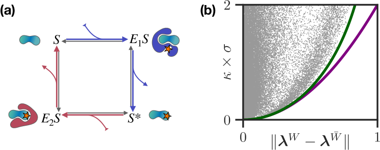
Figure 1: (a) Our results imply thermodynamic trade-offs with relaxation speed and oscillations in discrete-state systems, such as the 4-state “push-pull” model of enzyme concentration sensing owen2020universal . (b) Our thermodynamic bounds on the spectral perturbation (7) are illustrated on randomly sampled rate matrices. The far-from-equilibrium bound $\kappa\times\sigma\geq 2\|\Delta\boldsymbol{\lambda}\|\operatorname{\tanh^{-1}}\|\Delta\boldsymbol{\lambda}\|$ is shown in green and the near-equilibrium bound $\kappa\times\sigma\geq 2\|\Delta\boldsymbol{\lambda}\|^{2}$ is shown in purple.

Given the importance of the spectrum in various functional properties, we ask whether there is any relationship between a system’s spectral and thermodynamic properties. In this paper, we prove the existence of this kind of relationship and explore some of its physical consequences. As one consequence, we demonstrate that steady-state EPR bounds the size of the spectral gap, implying a fundamental thermodynamic cost for fast relaxation and for rapid decay of autocorrelation. We also show that steady-state EPR bounds the size of the imaginary part of the spectrum, implying a fundamental thermodynamic cost for fast oscillations. Both consequences follow from a general relationship between thermodynamic cost and spectral perturbations, illustrated in Fig. 1(b). This general relationship shows that the steady-state EPR under the nonequilibrium rate matrix $W$ bounds the difference between the spectrum of $W$ and a “reference” equilibrium rate matrix $\bar{W}$, which has the same steady state and dynamical activity as $W$ but obeys detailed balance.

II Preliminaries

Given a rate matrix $W$ with steady-state $\boldsymbol{\pi}$, the steady-state EPR is defined as schnakenbergNetworkTheoryMicroscopic1976 ; van2015ensemble

$$\sigma:=\frac{1}{2}\sum_{i\neq j}(\pi_{i}W_{ji}-\pi_{j}W_{ij})\ln\frac{\pi_{i}W_{ji}}{\pi_{j}W_{ij}}\geq 0\,.$$ (3)

For simplicity, we assume that $W$ is irreducible and “weakly reversible” ($W_{ji}>0$ whenever $W_{ij}>0$) ensuring that $\boldsymbol{\pi}$ is unique and $\sigma$ is finite. The steady-state EPR vanishes when forward and backward probability fluxes balance for all $i,j$, $\pi_{i}W_{ji}=\pi_{j}W_{ij}$. This condition is termed detailed balance (DB), and we identify it with equilibrium.

The quantity $\sigma$ can be interpreted as the rate of increase of thermodynamic entropy when the master equation obeys “local detailed balance” (LDB). Formally, LDB holds if for each transition $i\to j$, the log-ratio $\ln({W_{ji}}/{W_{ij}})$ can be identified with the corresponding increase of thermodynamic entropy in the environment. (See Ref. maes_ldb_notes for more details and a microscopic derivation of LDB.) LDB can also be considered for coarse-grained systems Note100 ; esposito2012stochastic and systems in contact with multiple thermodynamic reservoirs esposito2010three , in which case $\sigma$ provides a lower bound on the rate of increase of thermodynamic entropy. If LDB does not hold, $\sigma$ can still serve as a useful information-theoretic measure of time irreversibility fodor2022irreversibility .

In our first result below, we relate $\sigma$ to the difference between the spectrum of the rate matrix $W$ and that of a “reference” rate matrix $\bar{W}_{ij}:=(W_{ij}+W_{ji}{\pi_{i}}/{\pi_{j}})/2$. The rate matrix $\bar{W}$ obeys DB while having many of the same dynamical properties as $W$: the same steady state $\boldsymbol{\pi}$, same escape rates $\bar{W}_{ii}=W_{ii}$, and same dynamical activity across each transition. The dynamical activity across transition $i\to j$ is the rate of back-and-forth jumps maes2020frenesy ,

$$\mathcal{A}_{ji}:=\pi_{i}W_{ji}+\pi_{j}W_{ij}=\pi_{i}\bar{W}_{ji}+\pi_{j}\bar{W}_{ij}.$$ (4)

The rate matrix $\bar{W}$ is the equilibrium analogue of $W$, and it is equal to $W$ if and only if $W$ obeys DB. It is sometimes called the “additive reversibilization” of $W$ in the literature sakai2016eigenvalue ; bremaud2001markov .

For any rate matrix such as $W$, we use $\boldsymbol{\lambda}^{W}$ to indicate the vector of eigenvalues of $W$ sorted in descending order by real part, $\mathrm{Re}\,\lambda_{1}^{W}\geq\dots\geq\mathrm{Re}\,\lambda_{n}^{W}$. We will study the spectral perturbation between $W$ and $\bar{W}$, i.e., the difference between their eigenvalues. There are some subtleties involved in quantifying this difference, since in general there is no canonical one-to-one mapping between the eigenmodes of these two matrices. Following previous work kahanSpectraNearlyHermitian1975 ; bhatiaMatrixAnalysis1997 , we quantify it in terms of the distance between the sorted eigenvalue vectors: $\|\Delta\boldsymbol{\lambda}\|:=\|\boldsymbol{\lambda}^{W}-\boldsymbol{\lambda}^{\bar{W}}\|$. Importantly, $\|\Delta\boldsymbol{\lambda}\|$ is the minimal distance across all possible one-to-one mappings between the eigenvalues, $\|\Delta\boldsymbol{\lambda}\|=\min_{\Pi}\|\boldsymbol{\lambda}^{W}-\Pi\boldsymbol{\lambda}^{\bar{W}}\|$, where $\Pi$ runs over all permutation matrices . In physical terms, $\|\Delta\boldsymbol{\lambda}\|$ compares the slowest modes of $W$ with the slowest modes of $\bar{W}$, and the fastest modes with the fastest modes.

Finally, we introduce two rate constants that will play a central role in our analysis. The first rate constant, which we term the mixing rate, is defined as

$$\kappa :=\max_{i\neq j}\frac{\mathcal{A}_{ji}}{2\pi_{i}\pi_{j}}.$$ (5)

The mixing rate quantifies the maximum dynamical activity across any edge, after an appropriate normalization by the steady-state probabilities. As shown in Appendix A, it can be understood as the maximum speed with which probability can flow between different regions of state space. The second rate constant is

$$\eta_{W}:=\sqrt{\sum_{i\neq j}\pi_{i}\pi_{j}\Big{(}\frac{\mathcal{A}_{ji}}{2\pi_{i}\pi_{j}}\Big{)}^{2}}.$$ (6)

It reflects the overall magnitude of the normalized dynamical activity, where the contribution of each transition is weighted by the steady-state distribution. These two constants depend only on the dynamical activity and steady-state distribution and can be equivalently defined either in terms of $W$ or $\bar{W}$.

III Thermodynamic bound on spectral perturbations

In our first main result, we demonstrate that the steady-state EPR bounds the magnitude of the spectral perturbation $\|\Delta\boldsymbol{\lambda}\|=\|\boldsymbol{\lambda}^{W}-\boldsymbol{\lambda}^{\bar{W}}\|$ as

$$\frac{\sigma}{2\kappa} \geq\left(\frac{\eta_{W}}{\kappa}\right)^{2}\frac{\|\Delta\boldsymbol{\lambda}\|}{\eta_{W}}\operatorname{\tanh^{-1}}\frac{\|\Delta\boldsymbol{\lambda}\|}{\eta_{W}}\geq\frac{\|\Delta\boldsymbol{\lambda}\|^{2}}{\kappa^{2}}\,.$$ (7)

The first bound is derived using a classic spectral perturbation theorem from linear algebra kahanSpectraNearlyHermitian1975 , see derivation in Appendix C.1. The second bound follows from $x\operatorname{\tanh^{-1}}x\geq x^{2}$, which is tight for small $x$. The two bounds become equivalent near equilibrium, when $\sigma\approx 0$, $W\approx\bar{W}$, and $\|\Delta\boldsymbol{\lambda}\|\approx 0$.

Eq. (7) implies that there is a universal thermodynamic cost for having the eigenvalues of $W$ be different from those of its equilibrium analogue $\bar{W}$. Importantly, all terms that appear in our bounds ($\sigma$, $\kappa$, $\eta_{W}$, and $\|\Delta\boldsymbol{\lambda}\|$) are functions of the system’s rate matrix and they all have units of “per time”. Moreover, all of these terms increase in the same linear manner when the rate matrix is scaled as $W\mapsto\alpha W$. Therefore, the bounds (7) are invariant to the overall scaling of the rate matrix, depending instead only on its structure.

Observe that steady-state EPR (3) depends both on the system’s kinetic properties, via the fluxes $\pi_{i}W_{ji}-\pi_{j}W_{ij}$, and its thermodynamic properties, via the dimensionless ratios $\ln(\pi_{i}W_{ji}/\pi_{j}W_{ij})$ (which are called “thermodynamic forces” in the literature esposito2010three ). The rate constants $\eta_{W}$ and $\kappa$ serve as normalization terms for the kinetics, allowing EPR to be compared to the spectral perturbation in a dimensionless manner. Near equilibrium, only the mixing rate $\kappa$ plays a role, while the rate constant $\eta_{W}$ becomes relevant in the far-from-equilibrium regime. The dimensionless ratio ${\eta_{W}}/{\kappa}$ in (7) measures the disorder of the normalized dynamical activity, and it reaches its maximum when the values of $\mathcal{A}_{ji}/{2\pi_{i}\pi_{j}}$ are equal for all allowed transitions.

We illustrate our result in Fig. 1(b). We generate $10^{5}$ random 5-by-5 rate matrices, scaled to have $\eta_{W}=1$. We plot $\kappa\times\sigma$ versus two lower bounds that follow from (7): $2\|\Delta\boldsymbol{\lambda}\|\operatorname{\tanh^{-1}}\|\Delta\boldsymbol{\lambda}\|$ and $2\|\Delta\boldsymbol{\lambda}\|^{2}$. Observe that the first bound can be arbitrarily tight far from equilibrium. In fact, one can verify that it is saturated by unicyclic rate matrices with uniform rates.

We can also invert Eq. (7) to derive an upper bound on the spectral perturbation as a function of the EPR. Define the function $\Phi_{y}:\mathbb{R}_{\geq 0}\to\mathbb{R}_{\geq 0}$ as

$$\Phi_{y}(x):=2xy\operatorname{\tanh^{-1}}({x}/{y})\,,$$ (8)

so that (7) implies $\kappa\sigma\geq\Phi_{\eta_{W}}(\|\Delta\boldsymbol{\lambda}\|)$. We can then bound the spectral perturbation using EPR as

$$\|\Delta\boldsymbol{\lambda}\|\leq\Phi_{\eta_{W}}^{-1}(\kappa\sigma)\leq\sqrt{\frac{\kappa}{2}\sigma}\,,$$ (9)

where $\Phi_{\eta_{W}}^{-1}$ is the inverse function (which can be computed numerically from $\Phi_{\eta_{W}}$).

III.1 Intermediate bounds

The constant $\eta_{W}$ depends on the overall pattern of dynamical activity across all transitions, which can be difficult to access in practice. Below, it will be useful to derive more general bounds that do not depend on this constant. We define another rate matrix $G$,

$$G_{ij}:=\begin{cases}\pi_{i}&i\neq j,\,W_{ij}>0\\ 0&i\neq j,\,W_{ij}=0\end{cases}\qquad G_{ii}:=-\sum_{j(\neq i)}G_{ji}.$$ (10)

This rate matrix obeys DB and has the same steady-state distribution and the same graph topology as $W$ (the same pattern of allowed transitions with non-zero rates). At the same time, it does not depend on the dynamical activity under $W$. The constant $\eta_{W}$ can then be bound as

$$\eta_{W}\leq\kappa\eta_{G}\leq\kappa\sqrt{1-\sum_{i}\pi_{i}^{2}}\leq\kappa,$$ (11)

where $\eta_{G}$ is defined as in (6) but using $G$ instead of $W$ (see Appendix B). Plugging these inequalities into (9) and using that $\Phi_{y}^{-1}(x)$ is increasing in $y$ gives a hierarchy of inequalities which fall in-between the two expressions in (9):

$$\|\Delta\boldsymbol{\lambda}\|\leq\Phi_{\eta_{W}}^{-1}(\kappa\sigma)\leq\Phi_{\kappa\eta_{G}}^{-1}(\kappa\sigma)\leq..\leq\Phi_{\kappa}^{-1}(\kappa\sigma)\leq\sqrt{\frac{\kappa}{2}\sigma}.$$

Within this hierarchy, tighter bounds reflect finer-grained information about the rate matrix $W$. The weakest bounds depend only on the mixing rate $\kappa$, the intermediate bound also depends on the steady-state distribution and the graph topology (via $\eta_{G}$), while the tightest bound depends on the overall pattern of dynamical activity (via $\eta_{W}$). In principle, there are systems in which all the bounds expressed in terms of $\Phi_{y}^{-1}$ are tight far-from-equilibrium.

III.2 Real and imaginary eigenvalues

The spectral perturbation can be decomposed into contributions from the real and imaginary parts of each eigenvalue,

$$\|\Delta\boldsymbol{\lambda}\|^{2}=\sum_{\alpha=2}^{n}|\Delta\mathrm{Re}\,\lambda_{\alpha}|^{2}+\sum_{\alpha=2}^{n}|\mathrm{Im}\,\lambda_{\alpha}^{W}|^{2},$$ (12)

where $\Delta\mathrm{Re}\,\lambda_{\alpha}=\mathrm{Re}\,\lambda_{\alpha}^{W}-\lambda_{\alpha}^{\bar{W}}$. In this expression, we used $\lambda_{1}^{\bar{W}}=\lambda_{1}^{W}=0$ and that the eigenvalues of $\bar{W}$ are real valued (Appendix C).

In the following, we use our general results to study separate trade-offs between EPR versus decay timescales and EPR versus oscillations. Interestingly, (12) also implies a three-way trade-off between EPR, decay timescales, and oscillations, exploration of which we leave for future work.

IV Spectral gap

We now derive thermodynamic bounds on the spectral gap $|\mathrm{Re}\,\lambda_{2}^{W}|$, which controls the slowest decay timescale of relaxation and autocorrelation.

We first consider a thermodynamic bound on the increase of the spectral gap:

$$0\leq|\mathrm{Re}\,\lambda_{2}^{W}|-|\lambda_{2}^{\bar{W}}|\leq\Phi_{\eta_{W}}^{-1}(\kappa\sigma)\leq\sqrt{\frac{\kappa}{2}\sigma}.$$ (13)

Thus, accelerating decay timescales under $W$, relative to the equilibrium rate matrix $\bar{W}$, carries an unavoidable thermodynamic cost. Weaker but more general bounds can be derived by combining (13) with the inequalities (11).

We derive (13) by combining (9) with $\|\Delta\boldsymbol{\lambda}\|\geq|\Delta\mathrm{Re}\,\lambda_{2}|$, then using that the spectral gap of $W$ is always larger than the spectral gap of $\bar{W}$ (see Appendix C.2):

$$|\Delta\mathrm{Re}\,\lambda_{2}|=|\mathrm{Re}\,\lambda_{2}^{W}|-|\lambda_{2}^{\bar{W}}|\geq 0\,.$$ (14)

The inequality (14) has been previously used to motivate “irreversible Monte Carlo” schemes ichikiViolationDetailedBalance2013 ; suwa2010markov ; bierkens2016non ; diaconis2000analysis ; turitsyn2011irreversible ; chen2013accelerating ; takahashi2016conflict ; sakai2016eigenvalue ; kaiser2017acceleration ; ghimenti2022accelerating . We note that the upper bounds (13) are often not tight, since the inequality $\|\Delta\boldsymbol{\lambda}\|\geq|\Delta\mathrm{Re}\,\lambda_{2}|$ is usually not saturated.

It is often useful to bound the spectral gap of $W$ itself, rather than the increase of the spectral gap of $W$ relative to $\bar{W}$. To do so, we combine $\Phi_{\eta_{W}}^{-1}(\kappa\sigma)\leq\Phi_{\kappa\eta_{G}}^{-1}(\kappa\sigma)$, as follows from (11), with the following inequalities on the spectral gap of $\bar{W}$ (Appendix C.3):

$$|\lambda_{2}^{\bar{W}}|\leq\kappa|\lambda_{2}^{G}|\leq\kappa,$$ (15)

where $|\lambda_{2}^{G}|$ is the spectral gap of the rate matrix $G$ from (10). Combining with (13) and rearranging gives

$$|\mathrm{Re}\,\lambda_{2}^{W}|\leq\Phi_{\kappa\eta_{G}}^{-1}(\kappa\sigma)+\kappa|\lambda_{2}^{G}|\leq\sqrt{\frac{\kappa}{2}\sigma}+\kappa|\lambda_{2}^{G}|.$$ (16)

These bounds depend only on the mixing rate $\kappa$, steady state $\boldsymbol{\pi}$, and graph topology of the rate matrix. They include one term that is a thermodynamic cost, which depends on the EPR and vanishes in equilibrium, and a second “baseline” term, which does not vanish in equilibrium. Weaker but simpler bounds can also be derived using (11) and (15). For instance, we may derive bounds which depend only on the mixing rate as

$$|\mathrm{Re}\,\lambda_{2}^{W}|\leq\Phi_{\kappa}^{-1}(\kappa\sigma)+\kappa\leq\sqrt{\frac{\kappa}{2}\sigma}+\kappa.$$ (17)

Eqs. (16) and (17) together form our second main result.

IV.1 Example

We illustrate our bounds on the spectral gap by studying the thermodynamic cost of response speed in biomolecular sensing mehta2012energetic ; govern2014energy ; skoge2013chemical ; owen2020universal ; qian2003thermodynamic ; goldbeter1981amplified . We consider a 4-state system with a cyclic topology, Fig. 1(a), inspired by the “push-pull” enzymatic sensor in the regime of low substrate concentrations owen2020universal . Here, a substrate molecule can be either unmodified ${S}$ or modified ${S}^{*}$. Modification is catalyzed by enzyme $E_{1}$ via bound state $E_{1}S$, and demodification is catalyzed by enzyme $E_{2}$ via bound state $E_{2}S$.

The steady-state distribution depends on the concentrations of $E_{1}$ and $E_{2}$ and serves as the sensor readout. Following a change of enzyme concentrations, the sensor’s response speed is determined by the rate of relaxation toward the new steady state, which can be quantified using the spectral gap $|\mathrm{Re}\,\lambda_{2}^{W}|$. The same idea applies not only to the push-pull system but also other molecular sensors where the steady state reflects environmental parameters.

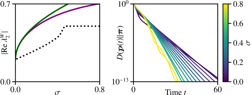
Figure 2: Thermodynamic bound on the spectral gap illustrated on the biomolecular sensing model from Fig. 1(a). Left: Two bounds from (16) (solid lines) versus the maximal spectral gap (dotted line) identified by numerical optimization at varying levels of steady-state EPR. Right: larger EPR is associated with faster relaxation to steady state, shown using the decay of KL divergence $D(\boldsymbol{p}(t)\|\boldsymbol{\pi})$ over time.

We use numerical optimization to find 4-by-4 cyclic rate matrices that have the largest spectral gap for a given steady-state EPR, given a fixed steady-state distribution $\boldsymbol{\pi}$ and mixing rate $\kappa$. For concreteness, we fix $\boldsymbol{\pi}=(0.4,0.1,0.4,0.1)$ and $\kappa=1$. Fig. 2(left) compares our bounds on the spectral gap (16) with the largest gap found by numerical optimization at different levels of EPR. Fig. 2(right) also shows that increased steady-state EPR is actually associated with faster relaxation. Specifically, using the rate matrices identified using numerical optimization, we plot $D(\boldsymbol{p}(t)\|\boldsymbol{\pi})=\sum_{i}p_{i}(t)\ln[p_{i}(t)/\pi_{i}]$. This is the Kullback–Leibler (KL) divergence between the time-dependent probability distribution $\boldsymbol{p}(t)$ (starting from $\boldsymbol{p}(0)=(1,0,0,0)$) and the steady state $\boldsymbol{\pi}$.

As seen in Fig. 2, our bounds are always satisfied but only saturate at $\sigma=0$. Interestingly, the spectral gap plateaus above $\sigma\approx 0.5$, when it reaches the largest value achievable for a given topology and steady state. Beyond this point, additional EPR leads to changes in other eigenvalues and increases the imaginary part of $\lambda_{2}$, as evidenced by oscillatory relaxation dynamics that emerge at large EPR in Fig. 2(right).

In future work, it may be interesting to relate our thermodynamic bound on response speed to existing thermodynamic bounds on sensitivity (ability of small parameter changes to elicit large changes in the steady state) mehta2012energetic ; govern2014energy ; skoge2013chemical ; owen2020universal ; qian2003thermodynamic .

V Imaginary eigenvalues

In our final set of main results, we show that the steady-state EPR bounds the magnitude of the entire imaginary part of the spectrum of $W$,

$$\|\mathrm{Im}\,\boldsymbol{\lambda}^{W}\|\leq\Phi_{\eta_{W}}^{-1}(\kappa\sigma)\leq\sqrt{\frac{\kappa}{2}\sigma},$$ (18)

where $\|\mathrm{Im}\,\boldsymbol{\lambda}^{W}\|=\sqrt{\sum_{\alpha=2}^{n}|\mathrm{Im}\,\lambda_{\alpha}^{W}|^{2}}$. This follows immediately from (9) and (12). Intermediate bounds which do not depend on the constant $\eta_{W}$ can be derived using (11).

We can also bound the imaginary part of any particular eigenmode (e.g., the slowest or the fastest). Consider the size of the imaginary part of any eigenvalue, $|\mathrm{Im}\,\lambda_{\alpha}^{W}|$ for $\alpha\in\{2,\dots,n\}$. Since nonreal eigenvalues come in conjugate pairs, there must be another eigenmode $\alpha^{\prime}$ with $|\mathrm{Im}\,\lambda_{\alpha^{\prime}}^{W}|=|\mathrm{Im}\,\lambda_{\alpha}^{W}|$. Given (12), we have $\|\mathrm{Im}\,\boldsymbol{\lambda}^{W}\|^{2}\geq 2|\mathrm{Im}\,\lambda_{\alpha}^{W}|^{2}$, which is tight for $n\leq 4$ and becomes increasingly weak for systems with many states. Plugging into (18) gives

$$|\mathrm{Im}\,\lambda_{\alpha}^{W}|\leq\frac{1}{\sqrt{2}}\Phi_{\eta_{W}}^{-1}(\kappa\sigma)\leq\sqrt{\frac{\kappa}{4}\sigma}.$$ (19)

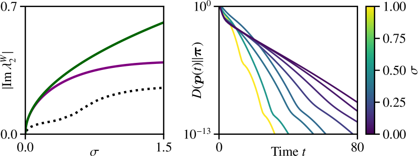
Figure 3: Thermodynamic bound on imaginary eigenvalues illustrated on the model from Fig. 1(a). Left: Two bounds from (19) (solid lines) versus the maximal imaginary part of the second eigenvalue (dotted line) identified by numerical optimization at varying levels of steady-state EPR. Right: larger EPR is associated with faster oscillatory “pulsing” during relaxation.

V.1 Example

As an illustration, we study the trade-off between steady-state EPR and oscillatory behavior, as quantified by the imaginary part of the slowest eigenmode, $|\mathrm{Im}\,\lambda_{2}^{W}|$. We again consider the 4-state cyclic system studied above, Fig. 1(a). Although oscillatory behavior is not typically desired in biomolecular sensors, it is necessary for other types of systems modeled using similar cyclic rate matrices, such as biochemical clocks barato2017coherence .

We use numerical optimization to find 4-by-4 cyclic rate matrices that maximize $|\mathrm{Im}\,\lambda_{2}^{W}|$ for a given EPR, given a fixed steady-state distribution and mixing rate $\kappa$ (chosen as above). In Fig. 3(left), we compare our bounds (19) with the largest imaginary part found by numerical optimization at different levels of steady-state EPR. In Fig. 3(right), we select some rate matrices identified using numerical optimization and plot $D(\boldsymbol{p}(t)\|\boldsymbol{\pi})=\sum_{i}p_{i}(t)\ln[p_{i}(t)/\pi_{i}]$. Observe that relaxation dynamics exhibit oscillatory “pulsing”, whose frequency increases with steady-state EPR.

VI Discussion

In this paper, we proved a relationship between the thermodynamic and spectral properties of a rate matrix. Our results on imaginary eigenvalues contribute to the extensive literature on the relationship between dissipation and oscillations barato2017coherence ; del2020high ; uhlAffinitydependentBoundSpectrum2019 ; oberreiter2021stochastic ; oberreiter2022universal ; ohga2023thermodynamic ; shiraishi2023entropy ; zheng2023topological .

More surprising, perhaps, is our thermodynamic bound on the real eigenvalues, including the increase of the spectral gap. This is because EPR quantifies the violation of time-reversal symmetry, which at first glance appears to be unrelated to the real part of the eigenvalues. These results contribute to the growing interest in time-symmetric phenomena maesTimeSymmetricFluctuationsNonequilibrium2006 ; maes2020frenesy ; baiesi2015inflow and relaxation timescales ghimenti2022accelerating ; bao2023universal ; teza2023eigenvalue ; dechant2023thermodynamic ; andrieuxSpectralSignatureNonequilibrium2011 as signatures of nonequilibrium.

In future work, it may be interesting to consider nonlinear systems, e.g., by studying the relationship between EPR and the Jacobian spectrum in deterministic chemical reaction networks. It is also interesting to extend our approach to continuous-state systems (Fokker–Planck generators) and open quantum systems (Lindblad generators). Interestingly, a recent preprint derived a different type of thermodynamic bound on relaxation in Fokker-Planck dynamics dechant2023thermodynamic ; comparison with our approach is left for future work.

APPENDIX A MEANING OF THE MIXING RATE $\kappa$

We show that the mixing rate $\kappa$, as defined in (5), can be understood as the maximum speed of probability flow between different regions of state space.

Consider any two subsets of states $\mathcal{X}\subseteq\{1,\dots,n\}$ and $\mathcal{Y}\subseteq\{1,\dots,n\}$. Let $T=e^{tW}$ indicate the time-$t$ transition matrix, and let $p_{\mathcal{X}\to\mathcal{Y}}(t)=\sum_{i\in\mathcal{X},j\in\mathcal{Y}}\pi_{i}T_{ji}$ indicate the probability that the steady-state process visits subset $\mathcal{X}$ at time $0$ and subset $\mathcal{Y}$ at time $t$. Since we assume that $W$ is irreducible, this probability converges to $p_{\mathcal{X}\to\mathcal{Y}}(\infty)=\sum_{i\in\mathcal{X},j\in\mathcal{Y}}\pi_{i}\pi_{j}$ in the long-time limit $t\to\infty$. Then, the mixing rate can be written as the normalized growth rate of $p_{\mathcal{X}\to\mathcal{Y}}(t)+p_{\mathcal{Y}\to\mathcal{X}}(t)$, maximized across all subsets:

$$\kappa=\max_{\mathcal{X},\mathcal{Y}}\frac{d}{dt}\frac{p_{\mathcal{X}\to\mathcal{Y}}(t)+p_{\mathcal{Y}\to\mathcal{X}}(t)}{p_{\mathcal{X}\to\mathcal{Y}}(\infty)+p_{\mathcal{Y}\to\mathcal{X}}(\infty)}\Big{|}_{t=0}.$$ (20)

To show the equivalence of (5) and (20), we first bound the numerator in (20) as

$$\frac{d}{dt}[p_{\mathcal{X}\to\mathcal{Y}}(t)+p_{\mathcal{Y}\to\mathcal{X}}(t)]\big{|}_{t=0}$$

$$\qquad\quad=\frac{d}{dt}\left[\sum_{i\in\mathcal{X},j\in\mathcal{Y}}(\pi_{i}T_{ji}+\pi_{j}T_{ij})\right]\Bigg{|}_{t=0}$$

$$\qquad\quad=\sum_{i\in\mathcal{X},j\in\mathcal{Y}}\pi_{i}W_{ji}+\pi_{j}W_{ij}$$

$$\qquad\quad\leq\left(\sum_{i\in\mathcal{X},j\in\mathcal{Y}}\pi_{i}\pi_{j}\right)\left(\max_{i\in\mathcal{X},j\in\mathcal{Y}}\frac{\pi_{i}W_{ji}+\pi_{j}W_{ij}}{\pi_{i}\pi_{j}}\right)$$

$$\qquad\quad=\left(\sum_{i\in\mathcal{X},j\in\mathcal{Y}}\pi_{i}\pi_{j}\right)\left(\max_{i\in\mathcal{X}\neq j\in\mathcal{Y}}\frac{\mathcal{A}_{ji}}{\pi_{i}\pi_{j}}\right).$$

In the last line, we used the definition of dynamical activity (4). We also restricted the maximization to $i\neq j$ by using the fact that $\mathcal{A}_{ii}\leq 0$ (since $W_{ii}\leq 0$). The denominator of the objective in (20) is given by

$$p_{\mathcal{X}\to\mathcal{Y}}(\infty)+p_{\mathcal{Y}\to\mathcal{X}}(\infty)=2\sum_{i\in\mathcal{X},j\in\mathcal{Y}}\pi_{i}\pi_{j}.$$

Combining gives the following upper bound on the right side of (20),

$$\max_{\mathcal{X}\neq\mathcal{Y}}\max_{i\in\mathcal{X}\neq j\in\mathcal{Y}}\frac{\mathcal{A}_{ji}}{2\pi_{i}\pi_{j}}\leq\max_{i\neq j}\frac{\mathcal{A}_{ji}}{2\pi_{i}\pi_{j}}.$$

where the last expression is the definition of $\kappa$ from (5). It can be verified that this upper bound is achieved by choosing $\mathcal{X}=\{i^{*}\}$ and $\mathcal{Y}=\{j^{*}\}$ in (20), where

$$(i^{*},j^{*})\in\operatorname*{\arg\,\max}_{i\neq j}\frac{\mathcal{A}_{ji}}{2\pi_{i}\pi_{j}}.$$

Therefore, (5) and (20) are equivalent.

APPENDIX B DERIVATION OF $\eta_{W}$ BOUNDS (LABEL:EQ:SEQ)

We first derive the following bound:

$$\eta_{W} =\sqrt{\sum_{i\neq j}\pi_{i}\pi_{j}\Bigg{(}\frac{\pi_{i}W_{ji}+\pi_{j}W_{ij}}{2\pi_{i}\pi_{j}}\Bigg{)}^{2}}$$

$$=\sqrt{\sum_{i\neq j:W_{ji}>0}\pi_{i}\pi_{j}\Bigg{(}\frac{\pi_{i}W_{ji}+\pi_{j}W_{ij}}{2\pi_{i}\pi_{j}}\Bigg{)}^{2}}$$

$$\leq\kappa\sqrt{\sum_{i\neq j:W_{ji}>0}\pi_{i}\pi_{j}}\,.$$

In the second line, we used the assumption $W$ is weakly reversible ($W_{ij}>0$ whenever $W_{ji}>0$), and in the last line we used the definition of $\kappa$ from (5). Next, observe that

$$\sqrt{\sum_{i\neq j:W_{ji}>0}\pi_{i}\pi_{j}}=\sqrt{\sum_{i\neq j}\pi_{i}\pi_{j}\Bigg{(}\frac{\pi_{i}G_{ji}+\pi_{j}G_{ij}}{2\pi_{i}\pi_{j}}\Bigg{)}^{2}}=\eta_{G},$$

where we used the definition of the rate matrix $G$ (10). Thus, we recover the first inequality in (11).

The second and third inequalities follow from

$$\sqrt{\sum_{i\neq j:W_{ji}>0}\pi_{i}\pi_{j}}\leq\sqrt{\sum_{i\neq j}\pi_{i}\pi_{j}}=\sqrt{1-\sum_{i}\pi_{i}^{2}}\leq 1.$$

APPENDIX C SPECTRAL INEQUALITIES

We begin by reviewing some of the notation and definitions introduced in the main text, along with a few useful results from linear algebra.

For any $n$-by-$n$ matrix $M$, we use the notation $\boldsymbol{\lambda}^{M}$ to indicate the vector of eigenvalues of matrix $M$ sorted in descending order by real part, $\mathrm{Re}\,\lambda_{1}^{M}\geq\dots\geq\mathrm{Re}\,\lambda_{n}^{M}$.

Given the rate matrix $W$, we define the reference equilibrium matrix

$$\bar{W}_{ij} :=\frac{1}{2}\big{(}W_{ij}+W_{ji}\frac{\pi_{i}}{\pi_{j}}\big{)}\,.$$ (21)

Assuming $W$ has a unique steady-state distribution $\boldsymbol{\pi}$, the first eigenvalue is $\lambda_{1}^{W}=0$, and $\mathrm{Re}\,\lambda_{\alpha}^{W}<0$ for all $\alpha\in\{2,\dots,n\}$. The right eigenvector corresponding to $\lambda_{1}^{W}$ is $\boldsymbol{\pi}=(\pi_{1},\dots,\pi_{n})^{T}$ so that $W\boldsymbol{\pi}=0$. The corresponding left eigenvector is $\boldsymbol{1}=(1,\dots,1)^{T}$ so that $\boldsymbol{1}^{T}W=0$. Any other right eigenvectors are orthogonal to $\boldsymbol{1}$, and any other left eigenvectors are orthogonal to $\boldsymbol{\pi}$. The same statements apply to $\bar{W}$ because it has the same unique steady-state distribution.

For convenience, we define the matrix

$$K_{ji} :=W_{ji}\sqrt{\pi_{i}/\pi_{j}}\,.$$ (22)

We write the Hermitian and anti-Hermitian parts of $K$ as

$$L:=\frac{1}{2}(K+K^{T})\qquad M:=\frac{1}{2}(K-K^{T}).$$ (23)

Introducing the diagonal matrix $D_{ji}=\delta_{ji}\sqrt{\pi_{i}}$, we can express $K$ and $L$ as similarity transformations of $W$ and $\bar{W}$ respectively, $K=D^{-1}WD$ and $L=D^{-1}\bar{W}D$. It then follows that they share the same spectra (hornMatrixAnalysis1990, , Cor. 1.3.4),

$$\boldsymbol{\lambda}^{K}=\boldsymbol{\lambda}^{W}\qquad\text{and}\qquad\boldsymbol{\lambda}^{L}=\boldsymbol{\lambda}^{\bar{W}}.$$ (24)

Note that $L$ is Hermitian, thus $\boldsymbol{\lambda}^{L}$ and $\boldsymbol{\lambda}^{\bar{W}}$ are real-valued. In addition, the second eigenvalue of $L$ obeys the variational principle (hornMatrixAnalysis1990, , Sec. 4.2)

$$\lambda_{2}^{L}=\max_{\boldsymbol{v}\in\mathbb{C}^{n}:\;\boldsymbol{v}\perp\sqrt{\boldsymbol{\pi}},\|\boldsymbol{v}\|=1}{\boldsymbol{v}}^{\dagger}L{\boldsymbol{v}}\,,$$ (25)

where $\sqrt{\boldsymbol{\pi}}:=(\sqrt{\pi_{1}},\dots,\sqrt{\pi_{n}})^{T}$ and the notation $\boldsymbol{a}\perp\boldsymbol{b}$ indicates orthogonality, $\sum_{i}a_{i}b_{i}=0$.

C.1 Derivation of first main result (7)

We first plug the definitions of $L$ and $M$ from (22) and (23) into the definition of steady-state EPR, which appears as (3) in the main text. After a bit of rearranging, this gives

$$\sigma =\sum_{i\neq j}2\sqrt{\pi_{i}\pi_{j}}|M_{ji}|\operatorname{\tanh^{-1}}\frac{|M_{ji}|}{L_{ji}}$$

$$\geq\frac{2}{\kappa}\sum_{i\neq j}L_{ji}|M_{ji}|\operatorname{\tanh^{-1}}\frac{|M_{ji}|}{L_{ji}}$$

$$\geq\frac{2}{\kappa}\Big{(}\sum_{i\neq j}L_{ji}|M_{ji}|\Big{)}\operatorname{\tanh^{-1}}\frac{\sum_{i\neq j}M_{ji}^{2}}{\sum_{i\neq j}L_{ji}|M_{ji}|}.$$ (26)

The second line uses $\sqrt{\pi_{i}\pi_{j}}\geq L_{ji}/\kappa$, where $\kappa$ is defined in (5). The third line applies Jensen’s inequality to the convex function $\operatorname{\tanh^{-1}}x$ (for $x\geq 0)$ with weights $L_{ji}|M_{ji}|/(\sum_{i\neq j}L_{ji}|M_{ji}|)$. Applying the Cauchy–Schwarz inequality then gives

$$\sum_{i\neq j}L_{ji}|M_{ji}|\leq\sqrt{\sum_{i\neq j}L_{ji}^{2}}\sqrt{\sum_{i\neq j}M_{ji}^{2}}=\eta_{W}\,\|M\|_{F},$$ (27)

where we used $\eta_{W}$ from (6) and the Frobenious norm $\|\cdot\|_{F}$.

We now combine (26) and (27), while using that $x\operatorname{\tanh^{-1}}(y/x)$ is decreasing in $x$ for $x,y\geq 0$. After a bit of rearranging, this gives

$$\frac{\sigma}{2\kappa}\geq\left(\frac{\eta_{W}}{\kappa}\right)^{2}\,\frac{\|M\|_{F}}{\eta_{W}}\operatorname{\tanh^{-1}}\frac{\|M\|_{F}}{\eta_{W}}.$$ (28)

Next, we will use the following classic theorem by Kahan (kahanSpectraNearlyHermitian1975, ), which we state here without proof and using our own notation.

Theorem. For Hermitian $L\in\mathbb{C}^{n\times n}$ and any $M\in\mathbb{C}^{n\times n}$,

$$\|\boldsymbol{\lambda}^{L}-\mathrm{Re}\,\boldsymbol{\lambda}^{L+M}\|\leq$$

$$\qquad\Big{\|}\frac{M+M^{\dagger}}{2}\Big{\|}_{F}+\sqrt{\Big{\|}\frac{M-M^{\dagger}}{2}\Big{\|}_{F}^{2}-\|\mathrm{Im}\,\boldsymbol{\lambda}^{L+M}\|^{2}}.$$

Observe that $L+M=K$, which follows from our definitions (23). Moreover, $M$ is anti-Hermitian, so $\|(M+M^{\dagger})/2\|_{F}=0$ and $\|(M-M^{\dagger})/2\|_{F}=\|M\|_{F}$. Combining with the theorem above and rearranging gives

$$\|M\|_{F}^{2} \geq\|\boldsymbol{\lambda}^{L}-\mathrm{Re}\,\boldsymbol{\lambda}^{K}\|^{2}+\|\mathrm{Im}\,\boldsymbol{\lambda}^{K}\|^{2}$$

$$=\|\boldsymbol{\lambda}^{L}-\boldsymbol{\lambda}^{K}\|^{2}=\big{\|}\boldsymbol{\lambda}^{W}-\boldsymbol{\lambda}^{\bar{W}}\big{\|}^{2}.$$ (29)

In the last line, we used that $\mathrm{Im}\,\boldsymbol{\lambda}^{L}=0$ since $L$ is Hermitian, and then used Eq. (24).

The result (7) follows by combining Eqs. (28) and (29), while using that $x\operatorname{\tanh^{-1}}x$ is decreasing in $x\geq 0$.

C.2 Derivation of the spectral gap inequality (14)

Let $\boldsymbol{u}$ be the right eigenvector of $K$ corresponding to $\lambda_{2}^{K}$, normalized so that $\|\boldsymbol{u}\|=1$. Using $K\boldsymbol{u}=\lambda_{2}^{K}\boldsymbol{u}$ and $\boldsymbol{u}^{\dagger}K^{T}=(\lambda_{2}^{K})^{*}\boldsymbol{u}^{\dagger}$, we can express the real part of the eigenvalue as

$$\mathrm{Re}\,\lambda_{2}^{K}=\frac{1}{2}\boldsymbol{u}^{\dagger}(K+K^{T})\boldsymbol{u}={\boldsymbol{u}}^{\dagger}L\boldsymbol{u}.$$ (30)

Since $K=D^{-1}WD$ and $\boldsymbol{1}^{T}W=0$, $K$ has a left eigenvector $(\boldsymbol{1}^{T}D)^{T}=\sqrt{\boldsymbol{\pi}}$ with the corresponding eigenvalue $\lambda_{1}^{K}=0$. The vector $\boldsymbol{u}$ is orthogonal to this eigenvector, $\boldsymbol{u}\perp\sqrt{\boldsymbol{\pi}}$. Therefore, $\boldsymbol{u}$ satisfies the constraints of the maximization (25). Combining (24), (25), and (30) then gives

$$\lambda_{2}^{\bar{W}}=\lambda_{2}^{L}\geq{\boldsymbol{u}}^{\dagger}L\boldsymbol{u}=\mathrm{Re}\,\lambda_{2}^{K}=\mathrm{Re}\,\lambda_{2}^{W}.$$ (31)

Finally, to derive (14), note that $\bar{W}$ and $W$ are rate matrices, thus $\lambda_{2}^{\bar{W}}\leq 0$ and $\mathrm{Re}\,\lambda_{2}^{W}\leq 0$.

We emphasize that the inequality (31) is known in the literature on irreversible Monte Carlo methods (ichikiViolationDetailedBalance2013, ; suwa2010markov, ; bierkens2016non, ; diaconis2000analysis, ; turitsyn2011irreversible, ; chen2013accelerating, ; takahashi2016conflict, ; sakai2016eigenvalue, ; kaiser2017acceleration, ; ghimenti2022accelerating, ). The derivation above is provided for completeness.

C.3 Derivation of spectral gap inequalities (15)

Using $|\lambda_{2}^{\bar{W}}|=|\lambda_{2}^{L}|=-\lambda_{2}^{L}$ and the variational principle (25), we write

$$|\lambda_{2}^{\bar{W}}| =-\max_{\boldsymbol{v}:\,\boldsymbol{v}\perp\sqrt{\boldsymbol{\pi}},\|\boldsymbol{v}\|=1}\sum_{ij}v_{i}^{*}L_{ij}v_{j}$$

$$=-\max_{\boldsymbol{v}:\,\boldsymbol{v}\perp\sqrt{\boldsymbol{\pi}},\|\boldsymbol{v}\|=1}\sum_{ij}\frac{v_{i}^{*}v_{j}}{\sqrt{\pi_{i}\pi_{j}}}\bar{W}_{ij}\pi_{j},$$

where we used that $L_{ij}=\bar{W}_{ij}\sqrt{\pi_{j}/\pi_{i}}$, as follows from our definitions (21), (22), and (23).

Next, we introduce the variables

$$\phi_{i}:=v_{i}/\sqrt{\pi_{i}}$$

and the norm

$$\|\boldsymbol{\phi}\|_{\boldsymbol{\pi}}=\sqrt{\sum_{i}|\phi_{i}|^{2}\pi_{i}}\,.$$

This allows us to rewrite

$$|\lambda_{2}^{\bar{W}}| =-\max_{\boldsymbol{\phi}:\,\boldsymbol{\phi}\perp\boldsymbol{\pi},\|\boldsymbol{\phi}\|_{\boldsymbol{\pi}}=1}\sum_{ij}\phi_{i}^{*}\phi_{j}\bar{W}_{ij}\pi_{j}$$

$$=\frac{1}{2}\min_{\boldsymbol{\phi}:\,\boldsymbol{\phi}\perp\boldsymbol{\pi},\|\boldsymbol{\phi}\|_{\boldsymbol{\pi}}=1}\sum_{i\neq j}|\phi_{i}-\phi_{j}|^{2}\bar{W}_{ij}\pi_{j},$$

where the second line follows from $\bar{W}_{ii}=-\sum_{j:\,j\neq i}\bar{W}_{ji}$ and the detailed balance condition $\bar{W}_{ij}\pi_{j}=\bar{W}_{ji}\pi_{i}$. Using

$$\bar{W}_{ij}\pi_{j}=\frac{W_{ij}\pi_{j}+W_{ji}\pi_{i}}{2\pi_{i}\pi_{j}}\pi_{i}\pi_{j}\leq\kappa G_{ij}\pi_{j}\leq\kappa\pi_{i}\pi_{j},$$

we can bound $|\lambda_{2}^{\bar{W}}|$ as

$$|\lambda_{2}^{\bar{W}}| \leq\frac{\kappa}{2}\min_{\boldsymbol{\phi}:\,\boldsymbol{\phi}\perp\boldsymbol{\pi},\|\boldsymbol{\phi}\|_{\boldsymbol{\pi}}=1}\sum_{i\neq j}|\phi_{i}-\phi_{j}|^{2}G_{ij}\pi_{j}=\kappa|\lambda_{2}^{G}|$$

$$\leq\frac{\kappa}{2}\min_{\boldsymbol{\phi}:\,\boldsymbol{\phi}\perp\boldsymbol{\pi},\|\boldsymbol{\phi}\|_{\boldsymbol{\pi}}=1}\sum_{i\neq j}|\phi_{i}-\phi_{j}|^{2}\pi_{i}\pi_{j}=\kappa,$$

where the last equality follows from $\frac{1}{2}\sum_{ij}|\phi_{i}-\phi_{j}|^{2}\pi_{i}\pi_{j}=1$ for any $\boldsymbol{\phi}$ that satisfies $\sum_{i}\phi_{i}\pi_{i}=0$ and $\sum_{i}|\phi_{i}|^{2}\pi_{i}=1$. This recovers the inequalities (15).

References

- (1) Y. Dou, K. Dhatt-Gauthier, and K. J. Bishop, “Thermodynamic costs of dynamic function in active soft matter,” Current Opinion in Solid State and Materials Science, vol. 23, no. 1, pp. 28–40, 2019.
- (2) P. Mehta, A. H. Lang, and D. J. Schwab, “Landauer in the age of synthetic biology: energy consumption and information processing in biochemical networks,” Journal of Statistical Physics, vol. 162, no. 5, pp. 1153–1166, 2016.
- (3) C. Van den Broeck and M. Esposito, “Ensemble and trajectory thermodynamics: A brief introduction,” Physica A: Statistical Mechanics and its Applications, vol. 418, pp. 6–16, 2015.
- (4) É. Fodor, R. L. Jack, and M. E. Cates, “Irreversibility and biased ensembles in active matter: Insights from stochastic thermodynamics,” Annual Review of Condensed Matter Physics, vol. 13, pp. 215–238, 2022.
- (5) J. J. Hopfield, “Kinetic proofreading: a new mechanism for reducing errors in biosynthetic processes requiring high specificity,” Proceedings of the National Academy of Sciences, vol. 71, no. 10, pp. 4135–4139, 1974.
- (6) P. Sartori and S. Pigolotti, “Thermodynamics of error correction,” Physical Review X, vol. 5, no. 4, p. 041039, 2015.
- (7) J. A. Owen, T. R. Gingrich, and J. M. Horowitz, “Universal thermodynamic bounds on nonequilibrium response with biochemical applications,” Physical Review X, vol. 10, no. 1, p. 011066, 2020.
- (8) J. M. Horowitz and T. R. Gingrich, “Thermodynamic uncertainty relations constrain non-equilibrium fluctuations,” Nature Physics, vol. 16, no. 1, pp. 15–20, 2020.
- (9) J. Schnakenberg, “Network theory of microscopic and macroscopic behavior of master equation systems,” Reviews of Modern physics, vol. 48, no. 4, p. 571, 1976.
- (10) N. G. Van Kampen, Stochastic processes in physics and chemistry. Elsevier, 1992, vol. 1.
- (11) L. J. Allen, An introduction to stochastic processes with applications to biology. CRC press, 2010.
- (12) If is not diagonalizable, it can still be written using the Jordan-Chevalley decomposition as the sum of two commuting matrices , with diagonalizable and nilpotent. Then , where can be decomposed as in Eq. (1) while contributes a factor that is polynomial in goudon2017math . A sufficient (but not necessary) condition for to be diagonalizable is having non-degenerate eigenvalues.
- (13) T. Goudon, Mathematics for modeling and scientific computing. Iste Ltd, 2016.
- (14) A. C. Barato and U. Seifert, “Coherence of biochemical oscillations is bounded by driving force and network topology,” Physical Review E, vol. 95, no. 6, p. 062409, 2017.
- (15) L. Oberreiter, U. Seifert, and A. C. Barato, “Universal minimal cost of coherent biochemical oscillations,” Physical Review E, vol. 106, no. 1, p. 014106, 2022.
- (16) N. O. Hodas, “The quality of oscillations in overdamped networks,” arXiv preprint arXiv:1006.0271, 2010.
- (17) M. Polettini, “Fisher information of Markovian decay modes: Nonequilibrium equivalence principle, dynamical phase transitions and coarse graining,” The European Physical Journal B, vol. 87, no. 9, p. 215, Sep. 2014.
- (18) D. Andrieux, “Spectral signature of nonequilibrium conditions,” Mar. 2011, arXiv:1103.2243 [cond-mat].
- (19) G. Teza, R. Yaacoby, and O. Raz, “Eigenvalue crossing as a phase transition in relaxation dynamics,” Physical Review Letters, vol. 130, no. 20, p. 207103, 2023.
- (20) H. Qian and M. Qian, “Pumped biochemical reactions, nonequilibrium circulation, and stochastic resonance,” Physical Review Letters, vol. 84, no. 10, p. 2271, 2000.
- (21) N. Ohga, S. Ito, and A. Kolchinsky, “Thermodynamic bound on the asymmetry of cross-correlations,” Physical Review Letters, vol. 131, no. 7, p. 077101, 2023.
- (22) F. Mancini, C. H. Wiggins, M. Marsili, and A. M. Walczak, “Time-dependent information transmission in a model regulatory circuit,” Physical Review E, vol. 88, no. 2, p. 022708, 2013.
- (23) T. Munakata and M. Kamiyabu, “Stochastic resonance in the fitzhugh-nagumo model from a dynamic mutual information point of view,” The European Physical Journal B-Condensed Matter and Complex Systems, vol. 53, pp. 239–243, 2006.
- (24) F. Tostevin and P. R. Ten Wolde, “Mutual information between input and output trajectories of biochemical networks,” Physical review letters, vol. 102, no. 21, p. 218101, 2009.
- (25) C. Jia and R. Grima, “Dynamical phase diagram of an auto-regulating gene in fast switching conditions,” The Journal of chemical physics, vol. 152, no. 17, 2020.
- (26) A. Y. Mitrophanov, “The spectral gap and perturbation bounds for reversible continuous-time Markov chains,” Journal of applied probability, vol. 41, no. 4, pp. 1219–1222, 2004.
- (27) C. Del Junco and S. Vaikuntanathan, “High chemical affinity increases the robustness of biochemical oscillations,” Physical Review E, vol. 101, no. 1, p. 012410, 2020.
- (28) M. Uhl and U. Seifert, “Affinity-dependent bound on the spectrum of stochastic matrices,” Journal of Physics A: Mathematical and Theoretical, vol. 52, no. 40, p. 405002, Oct. 2019.
- (29) L. Oberreiter, U. Seifert, and A. C. Barato, “Stochastic discrete time crystals: Entropy production and subharmonic synchronization,” Physical Review Letters, vol. 126, no. 2, p. 020603, 2021.
- (30) N. Shiraishi, “Entropy production limits all fluctuation oscillations,” Physical Review E, vol. 108, no. 4, p. L042103, 2023.
- (31) C. Zheng and E. Tang, “A topological mechanism for robust and efficient global oscillations in biological networks,” arXiv preprint arXiv:2302.11503, 2023.
- (32) C. Maes, “Local detailed balance,” SciPost Phys. Lect. Notes, p. 32, 2021.
- (33) Our spectral perturbation bounds are applicable to coarse-grained systems that are Markovian, so that their relaxation dynamics and autocorrelation functions can still be characterized by a rate matrix.
- (34) M. Esposito, “Stochastic thermodynamics under coarse graining,” Physical Review E, vol. 85, no. 4, p. 041125, 2012.
- (35) M. Esposito and C. Van den Broeck, “Three faces of the second law. I. Master equation formulation,” Physical Review E, vol. 82, no. 1, p. 011143, 2010.
- (36) C. Maes, “Frenesy: Time-symmetric dynamical activity in nonequilibria,” Physics Reports, vol. 850, pp. 1–33, 2020.
- (37) Y. Sakai and K. Hukushima, “Eigenvalue analysis of an irreversible random walk with skew detailed balance conditions,” Physical Review E, vol. 93, no. 4, p. 043318, 2016.
- (38) P. Brémaud, Markov chains: Gibbs fields, Monte Carlo simulation, and queues. Springer Science & Business Media, 2001, vol. 31.
- (39) W. Kahan, “Spectra of nearly Hermitian matrices,” Proceedings of the American Mathematical Society, vol. 48, no. 1, pp. 11–17, 1975.
- (40) R. Bhatia, Matrix Analysis. Springer, 1997.
- (41) This follows because has a real-valued spectrum. For details, see (bhatiaMatrixAnalysis1997, , p. 166).
- (42) A. Ichiki and M. Ohzeki, “Violation of detailed balance accelerates relaxation,” Physical Review E, vol. 88, no. 2, p. 020101, Aug. 2013.
- (43) H. Suwa and S. Todo, “Markov chain Monte Carlo method without detailed balance,” Physical Review Letters, vol. 105, no. 12, p. 120603, 2010.
- (44) J. Bierkens, “Non-reversible Metropolis-Hastings,” Statistics and Computing, vol. 26, no. 6, pp. 1213–1228, 2016.
- (45) P. Diaconis, S. Holmes, and R. M. Neal, “Analysis of a nonreversible Markov chain sampler,” Annals of Applied Probability, pp. 726–752, 2000.
- (46) K. S. Turitsyn, M. Chertkov, and M. Vucelja, “Irreversible Monte Carlo algorithms for efficient sampling,” Physica D: Nonlinear Phenomena, vol. 240, no. 4-5, pp. 410–414, 2011.
- (47) T.-L. Chen and C.-R. Hwang, “Accelerating reversible Markov chains,” Statistics & Probability Letters, vol. 83, no. 9, pp. 1956–1962, 2013.
- (48) K. Takahashi and M. Ohzeki, “Conflict between fastest relaxation of a Markov process and detailed balance condition,” Physical Review E, vol. 93, no. 1, p. 012129, 2016.
- (49) M. Kaiser, R. L. Jack, and J. Zimmer, “Acceleration of convergence to equilibrium in Markov chains by breaking detailed balance,” Journal of Statistical Physics, vol. 168, pp. 259–287, 2017.
- (50) F. Ghimenti and F. van Wijland, “Accelerating, to some extent, the p-spin dynamics,” Physical Review E, vol. 105, no. 5, p. 054137, 2022.
- (51) P. Mehta and D. J. Schwab, “Energetic costs of cellular computation,” Proceedings of the National Academy of Sciences, vol. 109, no. 44, pp. 17 978–17 982, 2012.
- (52) C. C. Govern and P. R. ten Wolde, “Energy dissipation and noise correlations in biochemical sensing,” Physical review letters, vol. 113, no. 25, p. 258102, 2014.
- (53) M. Skoge, S. Naqvi, Y. Meir, and N. S. Wingreen, “Chemical sensing by nonequilibrium cooperative receptors,” Physical review letters, vol. 110, no. 24, p. 248102, 2013.
- (54) H. Qian, “Thermodynamic and kinetic analysis of sensitivity amplification in biological signal transduction,” Biophysical chemistry, vol. 105, no. 2-3, pp. 585–593, 2003.
- (55) A. Goldbeter and D. E. Koshland Jr, “An amplified sensitivity arising from covalent modification in biological systems,” Proceedings of the National Academy of Sciences, vol. 78, no. 11, pp. 6840–6844, 1981.
- (56) C. Maes and M. H. Van Wieren, “Time-symmetric fluctuations in nonequilibrium systems,” Physical Review Letters, vol. 96, no. 24, p. 240601, Jun. 2006.
- (57) M. Baiesi and G. Falasco, “Inflow rate, a time-symmetric observable obeying fluctuation relations,” Physical Review E, vol. 92, no. 4, p. 042162, 2015.
- (58) R. Bao and Z. Hou, “Universal trade-off between irreversibility and relaxation timescale,” arXiv preprint arXiv:2303.06428, 2023.
- (59) A. Dechant, J. Garnier-Brun, and S.-i. Sasa, “Thermodynamic bounds on correlation times,” Physical Review Letters, vol. 131, no. 16, p. 167101, 2023.
- (60) R. A. Horn and C. R. Johnson, Matrix Analysis. Cambridge university press, 1990.