Energy-Saving Precoder Design for
Narrowband and Wideband Massive MIMO

Abstract

In this work, we study massive multiple-input multiple-output (MIMO) precoders optimizing power consumption while achieving the users’ rate requirements. We first characterize analytically the solutions for narrowband and wideband systems minimizing the power amplifiers (PAs) consumption in low system load, where the per-antenna power constraints are not binding. After, we focus on the asymptotic wideband regime. The power consumed by the whole base station (BS) and the high-load scenario are then also investigated. We obtain simple solutions, and the optimal strategy in the asymptotic case reduces to finding the optimal number of active antennas, relying on known precoders among the active antennas. Numerical results show that large savings in power consumption are achievable in the narrowband system by employing antenna selection, while all antennas need to be activated in the wideband system when considering only the PAs consumption, and this implies lower savings. When considering the overall BS power consumption and a large number of subcarriers, we show that significant savings are achievable in the low-load regime by using a subset of the BS antennas. While optimization based on transmit power pushes to activate all antennas, optimization based on consumed power activates a number of antennas proportional to the load.

I Introduction

I-A Problem Statement

The reduction of electrical energy consumption and carbon footprint is among the priorities of our society [1]. The information and communications technology (ICT) industry targets to reduce its greenhouse gas emissions by 45% by 2030 [2]. Moreover, decreasing the energy consumption of radio access networks lowers the operational expenses of operators, which have the largest impact on their bills [3]. Energy efficiency of mobile communications has been the object of research for more than a decade [4, 5, 6], but there is still room for improvement. Measurements [7, 8] show that the power consumption of current wireless networks does not depend much on data traffic and barely decreases even when the traffic is close to zero. This creates opportunities for energy savings: improving the load dependence of the consumption by, e.g., implementing adaptive shutdown of the network components [3, 7, 9]. Recent studies highlight how energy-saving gains up to 48.2% are achievable by only adapting the spatial transmission resources to the traffic [9].

The power amplifier (PA) is among the main contributors to the energy consumption of a base station (BS) [10], even though the share of the baseband processing is increasing in fifth-generation (5G) systems [11]. In orthogonal frequency-division multiplexing (OFDM), the current broadband modulation format used in cellular systems, the PA operates in linear regime to avoid signal distortion and out-of-band emissions. However, the PA efficiency is maximal when operating in the saturation region, leading to a trade-off between system capacity and power consumption [12]. Despite this, the conventional massive multiple-input multiple-output (MIMO) precoders are typically found by optimizing a certain figure of merit at the receivers, i.e., rate, signal-to-interference-plus-noise ratio (SINR), or mean square error (MSE), under a transmit power constraint [13]. Indeed, the maximal transmit power is commonly fixed by regulations. This would be optimal – in terms of PAs consumption – if the PA efficiency was fixed, but it actually depends on the output power level [14], making power consumption and transmit power not linearly proportional. Moreover, the optimization of the energy performance of existing precoders is traditionally based on their energy efficiency (EE), i.e., the number of transferred bits per unit of energy [15]. However, EE maximization does not guarantee a given quality-of-service (QoS) and can lead to undesirable situations, e.g., low power consumption but small rates, or large rates but equally high power consumption. An alternative approach is to fix the QoS requirements and minimize the power consumption. In this way, one can optimize the transmission resources for a specific traffic level, and avoid allocating too many resources when not necessary [9]. The above makes the trade-off between energy consumption and performance requirements transparent [3].

I-B State-of-the-Art

Considering a BS equipped with $M$ antennas, $p_{m}$ is defined as the power at the output of antenna $m$. The total transmit power is then given by $p_{\mathrm{tx}}=\sum_{m=0}^{M-1}p_{m}$. A common assumption is that the consumed power by the PA at antenna $m$ can be modeled as $\frac{p_{m}}{\eta}$, where $\eta$ is the fixed PA efficiency. In this way, the total power consumed by the PAs is linearly related to the total transmit power

$$p_{\mathrm{PAs}}^{\mathrm{(ideal)}}=\sum_{m=0}^{M-1}\frac{p_{m}}{\eta}=\frac{p_{\mathrm{tx}}}{\eta}.$$ (1)

However, (1) represents an ideal model. A more realistic expression of the efficiency of the PA $m$ is $\eta_{m}=\eta_{\mathrm{sat}}\left(\frac{p_{m}}{p_{\mathrm{sat}}}\right)^{1/2}$, where $p_{\mathrm{sat}}$ is the PA saturation power and $\eta_{\mathrm{sat}}$ is the maximal PA efficiency, achieved when $p_{m}=p_{\mathrm{sat}}$ [14]. This expression is accurate for class B amplifiers [16]. Considering also an industrial PA for 5G massive MIMO (mMIMO) [17], the square-root behavior proves to be suited to model the efficiency when far from saturation (e.g., considering a $10$ dB back-off). A back-off of $10$ dB is typically used in OFDM systems to operate in the linear regime [10], given the high peak-to-average power ratio (PAPR). Under this model, the total power consumed by the PAs becomes

$$p_{\mathrm{PAs}}=\sum_{m=0}^{M-1}\frac{p_{m}}{\eta_{m}}=\frac{p_{\mathrm{sat}}^{1/2}}{\eta_{\mathrm{sat}}}\sum_{m=0}^{M-1}p_{m}^{1/2}.$$ (2)

Despite the extensive research in mMIMO signal processing, few works have considered (2) in the precoders design, especially for a multicarrier system. In [18, 19], the authors analyzed the cases of multiple-input single-output (MISO) and MIMO with orthogonal channels. In the MISO case, the problem is formulated as minimization of (2) subject to a rate constraint and per-antenna power constraints. The solution corresponds to antenna selection, saturating the antennas with the largest channel gains and not activating the remaining antennas. The application to point-to-point MIMO is studied in [20], but the multi-user MIMO system is not investigated in detail. The work in [21] assumes the general form of the precoder (maximum ratio transmission (MRT) and zero-forcing (ZF) schemes) and finds a posteriori the system parameters (number of BS antennas, number of users, etc.) that minimize (2). They optimize the number of utilized BS antennas in a low-traffic regime, as in the high-traffic situation their choice is to always keep all the BS antennas turned on to guarantee the coverage in the cell. The solution (when considering only the power consumed by the PAs) is to activate all the BS antennas, in contrast to [18, 19]. The reason is that [18, 19] consider the minimization of (2) from the precoding problem definition, not assuming any particular precoding scheme. When other BS components are included in the power consumption model, the optimal number of BS antennas to be utilized decreases.

Similarly to [21], several studies have investigated the whole BS power consumption for energy-efficient mMIMO communications. A power consumption model for a mMIMO BS is developed in [22], where the total consumed power is the sum of the contributions from the PAs and from the BS circuits, plus a static consumption term. The circuit power consumption considers the radio frequency transceivers, the baseband processing, the backhauling, the cooling, and the power supply, and typically scales linearly with $M$ [22]. In [23], the authors jointly minimize the total transmit power and the circuit power consumption for MRT and ZF precoders. Differently from [21], they consider different traffic situations and they show that the number of activated antennas increases as a function of the traffic.

Remarkably, the multicarrier regime has not been investigated in enough detail in the literature. When considering a fixed PA efficiency, the definition (1) allows one to decouple and optimally solve the precoder design problem per-subcarrier. When optimizing the expression (2), instead, the problem is coupled between subcarriers as the PA efficiency depends on the total power at its input. The work [21] considers (2) in a mMIMO system assuming a uniform power among the antennas, given that each antenna serves a large number of subcarriers. Nonetheless, the form of the precoder is fixed a priori and this constitutes a limit in the analysis. The authors in [20] consider the case of point-to-point MIMO and optimize the sum-capacity subject to consumed power constraints and per-antenna power constraints. The expression of the consumed power takes into account the multicarrier nature of the system. Their conclusion is in line with ours (i.e., all the BS antennas are equally good, then random antenna selection performs well), but the analysis of the mMIMO scenario and further elaboration on how to optimize the parameters of the system are missing.

Available works have considered the maximization of the EE in MIMO precoding [24, 25], in some cases also considering a non-fixed PA efficiency [26, 27]. As previously mentioned, our approach does not focus on the EE, but fixes the rate requirements and derives the precoder that minimizes the power consumption. Indeed, conventional precoders can be obtained as solutions to optimization problems that minimize the transmit power subject to QoS constraints [13]. Therefore, one can optimize the transmission resources for an instance of QoS requirements, and repeat this process once the requirements change.

I-C Contributions

In this paper, we propose mMIMO precoders that minimize the consumed power under a zero inter-user interference constraint, starting from a general multi-user multicarrier system. The study is an extension of our previous work [28], where we only considered the PAs consumption and the single-carrier scenario (referred to as narrowband to underline that we consider the channel to be frequency flat). Our main contributions are:

• We derive closed-form solutions to the problem of minimizing the PAs consumption in wideband systems (Section III), where the powers at the BS antennas are computed via iterative fixed point algorithm. We focus on the low-load scenario, in which the antenna output powers are lower than the maximal PA power and the per-antenna power constraints are not binding.

• We characterize analytically the solutions to the same problem in narrowband systems and low load (Section IV), and we show that the single-user solution does not require an iterative method to be retrieved.

• We analyze the asymptotic behavior of wideband systems (Section V), solving the problem of minimizing the BS consumption subject to per-antenna power constraints. We derive the optimal number of active antennas, which depends on the traffic load.

In Section VI, the performance of the proposed solutions are evaluated numerically, and their complexity is discussed. Section VII concludes the paper.

Notations

Vectors and matrices are denoted by bold lowercase $\boldsymbol{\mathrm{a}}$ and uppercase letters $\boldsymbol{\mathrm{A}}$, respectively. The superscripts $(\cdot)^{*}$, $(\cdot)^{\mathrm{T}}$ and $(\cdot)^{\mathrm{H}}$ indicate complex conjugate, transpose, and conjugate transpose operations. The symbols $\mathrm{tr}\left(\cdot\right)$ and $\mathbb{E}\left\{\cdot\right\}$ indicate the trace and the expectation operators. The notation $\mathrm{diag}\left(\boldsymbol{\mathrm{a}}\right)$ refers to a diagonal matrix whose $k$-th diagonal entry is equal to the $k$-th element of $\boldsymbol{\mathrm{a}}$. A diagonal matrix associated with the vector $\boldsymbol{\mathrm{a}}$ is indicated by $\boldsymbol{\mathrm{D}}_{\boldsymbol{\mathrm{a}}}$. The identity matrix of size $K$ is $\boldsymbol{\mathrm{I}}_{K}$. The $(i,j)$-th element of $\boldsymbol{\mathrm{A}}$ is indicated by $\left[\boldsymbol{\mathrm{A}}\right]_{i,j}$. The notation $\mathcal{CN}(\mu,\sigma^{2})$ stands for a complex normal distribution with mean $\mu$ and variance $\sigma^{2}$. A complex Wishart distribution with mean $\boldsymbol{\mathrm{M}}$ and $n$ degrees of freedom is indicated by $\mathcal{CW}(\boldsymbol{\mathrm{M}},n,p)$, while a complex inverse Wishart distribution with mean $\boldsymbol{\mathrm{M}}\in\mathbb{C}^{p\times p}$ and $n$ degrees of freedom is denoted by $\mathcal{CW}^{-1}(\boldsymbol{\mathrm{M}},n,p)$. The symbol $\delta_{i,j}$ is the Kronecker delta function. If $f\colon\mathcal{X}\mapsto\mathbb{R}$ and $x\in\mathcal{X}$, $\lfloor x\rceil$ selects, among the two closest integers to $x$, the one associated to the minimum value of $f$. The matrix $\boldsymbol{\mathrm{A}}^{1/2}$ is the only Hermitian positive semidefinite matrix satisfying $\boldsymbol{\mathrm{A}}=\boldsymbol{\mathrm{A}}^{1/2}\boldsymbol{\mathrm{A}}^{1/2}$, $\boldsymbol{\mathrm{A}}^{n}$ is the multiplication of $n$ $\boldsymbol{\mathrm{A}}$ matrices and $\boldsymbol{\mathrm{A}}^{-n}$ is the multiplication of $n$ $\boldsymbol{\mathrm{A}}^{-1}$ matrices, for $n\in\mathbb{N}^{+}$. If $z=x+\jmath y$, with $x,y\in\mathbb{R}$, the Wirtinger derivative is defined as $\frac{\partial}{\partial z^{*}}=\frac{1}{2}\left(\frac{\partial}{\partial x}+\jmath\frac{\partial}{\partial y}\right)$. $\mathcal{O}(\cdot)$ stands for the big O notation.

II System Model

II-A Transmission Model

We consider the downlink of a single-cell mMIMO OFDM system with $Q$ subcarriers. The $M$ antennas at the BS serve $K$ single-antenna users using space-division multiplexing. The transmitted symbol for the user $k$ at the subcarrier $q$ is denoted by $s_{k,q}$, and the symbols are uncorrelated and of unit variance, i.e., $\mathbb{E}\left\{s_{k,q}s_{k^{\prime},q^{\prime}}^{*}\right\}=\delta_{k,k^{\prime}}\delta_{q,q^{\prime}}$. Indicating with $w_{m,k,q}$ the precoding coefficient for antenna $m$, user $k$ and subcarrier $q$, the precoded signal in the frequency domain at antenna $m$ and subcarrier $q$ is

$$x_{m,q}=\sum_{k=0}^{K-1}w_{m,k,q}s_{k,q}.$$ (3)

We assume the cyclic prefix to be sufficiently long and the channel to be time-invariant over an OFDM symbol period so that it can be considered flat at each subcarrier. Defining $h_{k,m,q}$ as the channel coefficient between user $k$ and antenna $m$ at subcarrier $q$, the signal received by the user $k$ at the subcarrier $q$ is

$$r_{k,q}=\sum_{m=0}^{M-1}h_{k,m,q}\sum_{k^{\prime}=0}^{K-1}w_{m,k^{\prime},q}s_{k^{\prime},q}+\nu_{k,q}$$ (4)

where $\nu_{k,q}\sim\mathcal{C}\mathcal{N}\left(0,\sigma_{\nu}^{2}\right)$ represents the thermal noise, which is assumed independently and identically distributed (i.i.d.) among subcarriers and users.

The above description represents a wideband multi-user scenario. The particular cases of narrowband and single-user systems are obtained for $Q=1$ and $K=1$, respectively. When we vary the number of subcarriers, the channel is assumed to remain flat at the subcarrier level. The underlying assumption is that the subcarrier spacing is fixed (i.e., the system bandwidth will decrease as a function of $Q$). The interest in analyzing a narrowband system is motivated, e.g., by the inclusion of services as narrowband IoT (NB-IoT) in the 5G standard [29].

II-B Power Consumption Model

Considering the precoded signal in (3), the transmit power at antenna $m$ equals

$$p_{m}=\sum_{q=0}^{Q-1}\mathbb{E}\left\{\left|x_{m,q}\right|^{2}\right\}=\sum_{k=0}^{K-1}\sum_{q=0}^{Q-1}\left|w_{m,k,q}\right|^{2}.$$ (5)

Consequently, the total transmit power at the BS is given by

$$p_{\mathrm{tx}}=\sum_{m=0}^{M-1}\sum_{q=0}^{Q-1}\mathbb{E}\left\{\left|x_{m,q}\right|^{2}\right\}=\sum_{m=0}^{M-1}\sum_{k=0}^{K-1}\sum_{q=0}^{Q-1}\left|w_{m,k,q}\right|^{2}.$$ (6)

Moreover, following the model in (2), the total power consumed by the PAs is given by

$$p_{\mathrm{PAs}}=\underbrace{\frac{p_{\mathrm{max}}^{1/2}}{\eta_{\mathrm{max}}}}_{\alpha}\sum_{m=0}^{M-1}\left(\sum_{k=0}^{K-1}\sum_{q=0}^{Q-1}\left|w_{m,k,q}\right|^{2}\right)^{1/2}.$$ (7)

Here and in the following, we consider $p_{\mathrm{max}}=\frac{p_{\mathrm{sat}}}{\mathrm{BO}}$ as the maximal PA’s power, where $\mathrm{BO}$ is the back-off (e.g., $\mathrm{BO}=10$), and $\eta_{\mathrm{max}}$ as the PA efficiency when $p_{m}=p_{\mathrm{max}}$. This choice is justified by the fact that a MIMO OFDM system must operate in the linear regime.

Expression (7) only considers the PAs contribution, while other BS components are also consuming. A simple, though appropriate, model of the BS power consumption is

$$p_{\mathrm{BS}}=p_{\mathrm{PAs}}+p_{\mathrm{fix}}+\mathcal{C}M_{\mathrm{a}}$$ (8)

where $p_{\mathrm{fix}}$ is the static power consumption, $\mathcal{C}$ is a positive linear scaling constant, and $M_{\mathrm{a}}\leq M$ is the number of active antennas (i.e., associated with a non-zero transmit power $p_{m}$). The term $\mathcal{C}M_{\mathrm{a}}$ accounts for the non-static contribution of the components other than the PAs, such as the transceiver chains and the baseband processing. A radio frequency (RF) transceiver chain comprises digital-to-analog converters (DACs), analog-to-digital converters (ADCs), filters, and mixers, and its consumption is either zero (non-active antenna) or equal to a constant value (active antenna). For common linear precoding schemes, the power consumption of the baseband unit is also linear in the number of active antennas [22]. It is worth pointing out that hybrid precoding strategies, using less RF chains than digital streams, enable the reduction of the BS consumption [31]. However, this paper focuses on fully digital architectures, which are typically used in sub-6 GHz systems.

II-C Assumptions

Some assumptions are made in certain sections of the paper:

$\mathbf{(As1)}$: low-load scenario, $p_{\mathrm{max}}\to\infty$.
We point out that, by letting $p_{\mathrm{max}}$ go to infinity, we practically mean that the constraints on the maximal power per antenna are not binding, as it usually happens in a low-load scenario. Indeed, if we define the load at antenna $m$ as the ratio $\frac{p_{m}}{p_{\mathrm{max}}}$, in a low-load scenario (i.e., with few users or low path loss) we expect that $p_{m}\ll p_{\mathrm{max}}\;\forall m$.

$\mathbf{(As2)}$: asymptotic wideband regime, $Q\to\infty$.
Also in this case, we underline that the results obtained by letting $Q$ go to infinity apply also for finite values of $Q$.

$\mathbf{(As3)}$: uncorrelated Rayleigh fading, $\boldsymbol{\mathrm{H}}_{q}=\boldsymbol{\mathrm{D}}_{\boldsymbol{\mathrm{\beta}}}^{1/2}\boldsymbol{\mathrm{G}}_{q}$,
where $\boldsymbol{\mathrm{H}}_{q}\in\mathbb{C}^{K\times M}$ is the channel matrix at subcarrier $q$, $\boldsymbol{\mathrm{D}}_{\boldsymbol{\mathrm{\beta}}}=\mathrm{diag}\left(\beta_{0},\dotsc,\beta_{K-1}\right)$ is the large-scale fading matrix and $\beta_{k}$ is the large-scale fading coefficient of user $k$. The matrix $\boldsymbol{\mathrm{G}}_{q}$ models the small-scale fading and is composed of i.i.d. elements, where the single entry is $g_{k,m,q}\sim\mathcal{C}\mathcal{N}\left(0,1\right)$. The i.i.d. assumption is made over space and not over frequency, therefore the channels of different subcarriers can be correlated.

III Precoders Design for Wideband System

III-A Traditional Transmit Power Solution

Denoting by $\gamma_{k}$ the target SINR for the user $k$, the precoder minimizing the total transmit power is the solution to

$$\operatorname*{minimize}_{\{w_{m,k,q}\}}\quad p_{\mathrm{tx}}=\sum_{m=0}^{M-1}p_{m}$$ (9)

$$\mathrm{subject\ to}\quad \boldsymbol{\mathrm{H}}_{q}\boldsymbol{\mathrm{W}}_{q}=\tilde{\boldsymbol{\mathrm{D}}}_{\boldsymbol{\mathrm{\gamma}}}^{1/2}\sigma_{\nu}\;\;\forall q,$$

$$p_{m}\leq p_{\mathrm{max}}\;\;\forall m$$

where $p_{m}$ is given by (5), $\boldsymbol{\mathrm{H}}_{q}\in\mathbb{C}^{K\times M}$ and $\boldsymbol{\mathrm{W}}_{q}\in\mathbb{C}^{M\times K}$ are the channel and precoding matrices at subcarrier $q$, respectively, $\tilde{\boldsymbol{\mathrm{D}}}_{\boldsymbol{\mathrm{\gamma}}}=\mathrm{diag}\left(\frac{\gamma_{0}}{Q},\dotsc,\frac{\gamma_{K-1}}{Q}\right)$ contains the target users’ SINRs normalized with respect to $Q$, and $\sigma_{\nu}$ is the noise standard deviation. The SINR at each subcarrier for user $k$ is then $\frac{\gamma_{k}}{Q}$. The first constraint is a ZF constraint, forcing the inter-user interference to zero. In the majority of the next sections, we rely on $\mathbf{(As1)}$ and we will relax the maximal power constraints.

The problem at hand is convex and differentiable. It can be solved by, e.g., the Lagrange multipliers method. Under $\mathbf{(As1)}$, the solution at the subcarrier $q$ is given by

$$\boldsymbol{\mathrm{W}}_{q}=\boldsymbol{\mathrm{H}}_{q}^{\mathrm{H}}\left(\boldsymbol{\mathrm{H}}_{q}\boldsymbol{\mathrm{H}}_{q}^{\mathrm{H}}\right)^{-1}\tilde{\boldsymbol{\mathrm{D}}}_{\boldsymbol{\mathrm{\gamma}}}^{1/2}\sigma_{\nu}$$ (10)

which corresponds to the per-subcarrier ZF [32]. Note that we consider instantaneous channel state information (CSI) to be available at the BS for the computation of the precoding matrices.

III-B PAs Consumed Power Solution

The precoder minimizing the total power consumed by the PAs is instead found by solving the following problem

$$\operatorname*{minimize}_{\{w_{m,k,q}\}}\quad p_{\mathrm{PAs}}=\alpha\sum_{m=0}^{M-1}p_{m}^{1/2}$$ (11)

$$\mathrm{subject\ to}\quad \boldsymbol{\mathrm{H}}_{q}\boldsymbol{\mathrm{W}}_{q}=\tilde{\boldsymbol{\mathrm{D}}}_{\boldsymbol{\mathrm{\gamma}}}^{1/2}\sigma_{\nu}\;\;\forall q,$$

$$p_{m}\leq p_{\mathrm{max}}\;\;\forall m.$$

As previously assumed to derive the conventional ZF, we consider $\mathbf{(As1)}$, thus neglecting the constraints on $p_{m}$. With this assumption, the transmit power at the individual antennas could become large. In practice, one can consider a rescaling of the rows of the precoding matrices corresponding to the antennas that are exceeding the maximum allowed power value, with the consequent reduction of the users’ SINR requirements. We focus on PA consumption because (i) the PA is usually one of the main drivers of the BS consumption [10], and (ii) the addition of other consumption terms would render the problem less tractable. However, in Section V we will show how the asymptotic analysis allows us to consider the BS consumption while remaining very accurate in practical situations with a finite realistic number of subcarriers.

The solution to the above problem can be found by, e.g., applying the Lagrange multipliers method, and is given in Theorem 1.

Theorem 1.

Under $(\mathbf{As1})$, the solution to problem (11) for the subcarrier $q$ is given by

$$\boldsymbol{\mathrm{W}}_{q}=\boldsymbol{\mathrm{D}}_{\boldsymbol{\mathrm{p}}}^{1/2}\boldsymbol{\mathrm{H}}_{q}^{\mathrm{H}}\left(\boldsymbol{\mathrm{H}}_{q}\boldsymbol{\mathrm{D}}_{\boldsymbol{\mathrm{p}}}^{1/2}\boldsymbol{\mathrm{H}}^{\mathrm{H}}_{q}\right)^{-1}\tilde{\boldsymbol{\mathrm{D}}}_{\boldsymbol{\mathrm{\gamma}}}^{1/2}\sigma_{\nu}$$ (12)

where $\boldsymbol{\mathrm{D}}_{\boldsymbol{\mathrm{p}}}=\mathrm{diag}\left(p_{0},\dotsc,p_{M-1}\right)=\mathrm{diag}(\boldsymbol{\mathrm{p}})$ is the matrix containing the transmit powers at the BS antennas, which are found by solving the fixed point equations

$$p_{m}=\sum_{k=0}^{K-1}\sum_{q=0}^{Q-1}\left|\left[\boldsymbol{\mathrm{D}}_{\boldsymbol{\mathrm{p}}}^{1/2}\boldsymbol{\mathrm{H}}_{q}^{\mathrm{H}}\left(\boldsymbol{\mathrm{H}}_{q}\boldsymbol{\mathrm{D}}_{\boldsymbol{\mathrm{p}}}^{1/2}\boldsymbol{\mathrm{H}}_{q}^{\mathrm{H}}\right)^{-1}\tilde{\boldsymbol{\mathrm{D}}}_{\boldsymbol{\mathrm{\gamma}}}^{1/2}\sigma_{\nu}\right]_{m,k}\right|^{2}$$ (13)

for $m=0,\dotsc,M-1$.

Proof.

See Appendix A. ∎

The system of fixed point equations can be solved through the fixed point iteration method, which is given in Algorithm 1. Once $\boldsymbol{\mathrm{D}}_{\boldsymbol{\mathrm{p}}}$ is known, it can be substituted in (12) to find the precoding matrices.

Algorithm 1 Fixed point method to retrieve the powers at the BS antennas

$\varepsilon,I_{\mathrm{max}}$ $\triangleright$ Set tolerance and max. number of iterations

$i\leftarrow 0$

for $m\in\{0,\dotsc,M-1\}$ do $\triangleright$ Init. powers at the BS antennas

    $p_{m}^{(0)}\leftarrow 1$

    $p_{m}^{(-1)}\leftarrow\infty$

end for

while $i<I_{\mathrm{max}}\textbf{ and }\max_{m}\left\{|p_{m}^{(i)}-p_{m}^{(i-1)}|\right\}>\varepsilon$ do

    $\boldsymbol{\mathrm{D}}_{\boldsymbol{\mathrm{p}}}\leftarrow\mathrm{diag}\left(p_{0}^{(i)},\dotsc,p_{M-1}^{(i)}\right)$

    for $m\in\{0,\dotsc,M-1\}$ do $\triangleright$ Update powers at the BS antennas

         $p_{m}^{(i+1)}\leftarrow(\ref{eq:MC-MU_fpe})$

    end for

    $i\leftarrow i+1$

end while

Let us now analyze the single-user case.

Corollary 1.

Under $\mathbf{(As1)}$, the particularization of Theorem 1 when $K=1$ gives the solution for the subcarrier $q$

$$\boldsymbol{\mathrm{w}}_{q}=\frac{\sigma_{\nu}\gamma^{1/2}}{Q^{1/2}}\frac{1}{\sum_{m^{\prime}=1}^{M-1}|h_{m^{\prime},q}|^{2}p_{m^{\prime}}^{1/2}}\boldsymbol{\mathrm{D}}_{\boldsymbol{\mathrm{p}}}^{1/2}\boldsymbol{\mathrm{h}}^{*}_{q}$$ (14)

where $\boldsymbol{\mathrm{w}}_{q}\in\mathbb{C}^{M\times 1}$ and $\boldsymbol{\mathrm{h}}_{q}\in\mathbb{C}^{M\times 1}$ are the precoding and channel vectors at the subcarrier $q$, respectively. The fixed point equations in the powers per antenna are

$$p_{m}=\frac{\sigma_{\nu}^{2}\gamma}{Q}p_{m}\sum_{q=0}^{Q-1}\frac{\left|h_{m,q}\right|^{2}}{\left(\sum_{m^{\prime}=0}^{M-1}\left|h_{m^{\prime},q}\right|^{2}p_{m^{\prime}}^{1/2}\right)^{2}}$$ (15)

for $m=0,\dotsc,M-1$.

In line-of-sight (LoS) channels, the problem simplifies and this allows us to draw interesting insights.

Corollary 2.

Under $\mathbf{(As1)}$, in pure LoS channels (i.e., characterized by $|h_{m,q}|=1\;\forall m,q$), and considering at least one $p_{m}$ different from zero, (15) reduces to

$$\sum_{m=0}^{M-1}p_{m}^{1/2}=\sigma_{\nu}\gamma^{1/2}.$$ (16)

Every transmit power allocation satisfying (16) is, therefore, an optimal solution to the wideband single-user problem in the low-load case, and thus also the narrowband single-user solution. One has now freedom in the precoder design. All the power can be allocated to antenna $m$, which will give $p_{m}=\sigma_{\nu}^{2}\gamma$. A uniform allocation is another possible choice, with $p_{m}=p=\frac{\sigma_{\nu}^{2}\gamma}{M^{2}}$. Random allocations are also doable, as long as they fulfill equation (16). In practice, however, it is better to activate the minimum number of antennas, so that the RF chains of the non-active antennas can be turned off to save power.

IV Narrowband System

IV-A Traditional Transmit Power Solution

When $Q=1$ the system reduces to a narrowband one. The subcarrier index $q$ is then discarded. The conventional solution, minimizing the total transmit power, corresponds to

$$\boldsymbol{\mathrm{W}}=\boldsymbol{\mathrm{H}}^{\mathrm{H}}\left(\boldsymbol{\mathrm{H}}\boldsymbol{\mathrm{H}}^{\mathrm{H}}\right)^{-1}\boldsymbol{\mathrm{D}}_{\boldsymbol{\mathrm{\gamma}}}^{1/2}\sigma_{\nu}$$ (17)

where $\boldsymbol{\mathrm{D}}_{\boldsymbol{\mathrm{\gamma}}}=\mathrm{diag}\left(\gamma_{0},\dotsc,\gamma_{K-1}\right)$, while $\boldsymbol{\mathrm{H}}\in\mathbb{C}^{K\times M}$ and $\boldsymbol{\mathrm{W}}\in\mathbb{C}^{M\times K}$ are the single-carrier channel and precoding matrices, respectively.

IV-B PAs Consumed Power Solution

Corollary 3.

Under $\mathbf{(As1)}$, it directly follows from Theorem 1 that the precoding matrix for a narrowband system is

$$\boldsymbol{\mathrm{W}}=\boldsymbol{\mathrm{D}}_{\boldsymbol{\mathrm{p}}}^{1/2}\boldsymbol{\mathrm{H}}^{\mathrm{H}}\left(\boldsymbol{\mathrm{H}}\boldsymbol{\mathrm{D}}_{\boldsymbol{\mathrm{p}}}^{1/2}\boldsymbol{\mathrm{H}}^{\mathrm{H}}\right)^{-1}\boldsymbol{\mathrm{D}}_{\boldsymbol{\mathrm{\gamma}}}^{1/2}\sigma_{\nu}.$$ (18)

The fixed point equation for the antenna $m$ is given by

$$p_{m}=\sum_{k=1}^{K}\left|\left[\boldsymbol{\mathrm{D}}_{\boldsymbol{\mathrm{p}}}^{1/2}\boldsymbol{\mathrm{H}}^{\mathrm{H}}\left(\boldsymbol{\mathrm{H}}\boldsymbol{\mathrm{D}}_{\boldsymbol{\mathrm{p}}}^{1/2}\boldsymbol{\mathrm{H}}^{\mathrm{H}}\right)^{-1}\boldsymbol{\mathrm{D}}_{\boldsymbol{\mathrm{\gamma}}}^{1/2}\sigma_{\nu}\right]_{m,k}\right|^{2}.$$ (19)

The solution can be retrieved in the same way as the wideband system, first computing the powers per antenna and substituting them in (18).

The single-user case can now be discussed.

Corollary 4.

Under $\mathbf{(As1)}$, by assuming different channel gains among the antennas and by defining $\hat{m}=\operatorname*{arg\,max}_{m}|h_{m}|$, the particularization of Corollary 1 when $Q=1$ gives the single-user solution

$$w_{m}=\begin{cases}\sigma_{\nu}\gamma^{1/2}\frac{1}{|h_{m}|^{2}}h_{m}^{*}&\mathrm{if}\ m=\hat{m}\\ 0&\mathrm{otherwise}\end{cases}.$$ (20)

All the power is therefore allocated to the antenna with the largest channel gain.

Proof.

From Corollary 1, when $Q=1$ we obtain

$$\boldsymbol{\mathrm{w}}=\sigma_{\nu}\gamma^{1/2}\frac{1}{\sum_{m^{\prime}=0}^{M-1}|h_{m^{\prime}}|^{2}p_{m^{\prime}}^{1/2}}\boldsymbol{\mathrm{D}}_{\boldsymbol{\mathrm{p}}}^{1/2}\boldsymbol{\mathrm{h}}^{*}$$ (21)

where $\boldsymbol{\mathrm{w}}\in\mathbb{C}^{M\times 1}$ and $\boldsymbol{\mathrm{h}}\in\mathbb{C}^{M\times 1}$ are the single-carrier precoding and channel vectors, respectively. The fixed point equation for the antenna $m$ is

$$\sum_{m^{\prime}=0}^{M-1}|h_{m^{\prime}}|^{2}p_{m^{\prime}}^{1/2}=\sigma_{\nu}\gamma^{1/2}|h_{m}|.$$ (22)

For all the activated antennas, there is a fixed point equation. However, when the channel gains $|h_{m}|$ are different, (22) cannot be solved since the left-hand side does not depend on $m$, while the right-hand side does. This actually shows that the optimal solution corresponds to using only one antenna, the one with the strongest channel gain [28]. This solution makes sense since the maximal per-antenna power constraint is not considered here. ∎

If several antennas share the same maximal channel gains, they can be all activated while still solving equation (22). Equation (22) reduces to equation (16) among the antennas sharing the same maximal channel gain. In pure LoS channels, we obtain again (16), this time among all the antennas. In both cases, one has freedom of choice in the precoder design.

When the per-antenna power constraints are active, instead, the optimal strategy is to progressively saturate the antennas with the highest channel gains until the QoS is achieved [18].

V Asymptotic Wideband System

We now assume a large value of $Q$, which makes sense given that in fourth-generation (4G) and 5G systems the number of active subcarriers varies from $72$ to $1320$ and from $132$ to $3300$, respectively [29]. The asymptotic results are validated numerically, and we show how they prove to be accurate even for a finite and relatively low number of subcarriers. The closed-form expressions of the consumed powers are obtained for the i.i.d. Rayleigh fading channel given in $\mathbf{(As3)}$.

V-A PAs Consumed Power

The following theorem gives the asymptotic expression of the PAs consumed power by the precoder (12). This characterization is possible because, in the asymptotic wideband regime, all the BS antennas are approximately allocated the same power.

Theorem 2.

Under $\mathbf{(As1)}-\mathbf{(As3)}$, the transmit power allocated to each antenna by the precoder (12) converges to

$$p_{m}\to\overline{p}=\frac{1}{M(M-K)}\mathrm{tr}\left(\boldsymbol{\mathrm{D}}_{\boldsymbol{\mathrm{\beta}}}^{-1}\boldsymbol{\mathrm{D}}_{\boldsymbol{\mathrm{\gamma}}}\sigma_{\nu}^{2}\right)$$ (23)

implying that the total power consumed by the PAs satisfies

$$p_{\mathrm{PAs}}\to\overline{p_{\mathrm{PAs}}}=\alpha\left(\frac{M}{M-K}\mathrm{tr}\left(\boldsymbol{\mathrm{D}}_{\boldsymbol{\mathrm{\beta}}}^{-1}\boldsymbol{\mathrm{D}}_{\boldsymbol{\mathrm{\gamma}}}\sigma_{\nu}^{2}\right)\right)^{1/2}.$$ (24)

The per-subcarrier ZF precoder is therefore found back

$$\boldsymbol{\mathrm{W}}_{q}=\boldsymbol{\mathrm{H}}_{q}^{\mathrm{H}}\left(\boldsymbol{\mathrm{H}}_{q}\boldsymbol{\mathrm{H}}_{q}^{\mathrm{H}}\right)^{-1}\tilde{\boldsymbol{\mathrm{D}}}_{\boldsymbol{\mathrm{\gamma}}}^{1/2}\sigma_{\nu}.$$ (25)

Proof.

See Appendix B. ∎

Looking at (24), the power consumed by the PAs is a monotonically decreasing function of $M$: activating more antennas is then always beneficial. However, the marginal gain of activating more antennas decreases as $M$ increases since $\frac{M}{M-K}$ converges to a unit constant.

V-B BS Consumed Power

Considering the power consumption of the BS, the optimal precoder does not necessarily activate all the antennas. Indeed, the power consumed by the BS circuits induces a penalty on the number of active antennas $M_{\mathrm{a}}$. The general problem, considering the BS consumption and the per-antenna power constraints, consists in solving

$$\operatorname*{minimize}_{\begin{subarray}{c}\{w_{m,k,q}\},M_{\mathrm{a}}\\ m=0,\dotsc,M_{\mathrm{a}}-1\end{subarray}}\quad p_{\mathrm{BS}}=\alpha\sum_{m=0}^{M_{\mathrm{a}}-1}p_{m}^{1/2}+p_{\mathrm{fix}}+\mathcal{C}M_{\mathrm{a}}$$ (26)

$$\mathrm{\ subject\ to}\quad \boldsymbol{\mathrm{H}}_{q}\boldsymbol{\mathrm{W}}_{q}=\tilde{\boldsymbol{\mathrm{D}}}_{\boldsymbol{\mathrm{\gamma}}}^{1/2}\sigma_{\nu}\;\;\forall q,$$

$$p_{m}\leq p_{\mathrm{max}}\;\;\forall m,$$

$$M_{\mathrm{a}}\leq M.$$

Without loss of generality, one can first optimize with respect to the precoding coefficients considering a generic number of active antennas $M_{\mathrm{a}}$, and then find the optimal integer number of active antennas.

Let us consider the power allocation defined in Theorem 2 among the $M_{\mathrm{a}}$ active antennas. By combining the BS consumption model in (8) with the asymptotic PAs consumption in (24), the asymptotic BS consumption is computed as

$$p_{\mathrm{BS}}\to\overline{p_{\mathrm{BS}}}=\alpha\left(\frac{M_{\mathrm{a}}}{M_{\mathrm{a}}-K}\mathrm{tr}\left(\boldsymbol{\mathrm{D}}_{\boldsymbol{\mathrm{\beta}}}^{-1}\boldsymbol{\mathrm{D}}_{\boldsymbol{\mathrm{\gamma}}}\sigma_{\nu}^{2}\right)\right)^{1/2}+p_{\mathrm{fix}}+\mathcal{C}M_{\mathrm{a}}.$$ (27)

The above quantity is the solution, under $\mathbf{(As1)-(As3)}$, to the minimization problem (26) with respect to the precoding coefficients and considering a fixed number of active antennas $M_{\mathrm{a}}$. The corresponding precoder is a per-subcarrier ZF precoder among the $M_{\mathrm{a}}$ active antennas.

We can now optimize the number of active antennas $M_{\mathrm{a}}$.

V-B1 Optimal $M_{\mathrm{a}}$ without Power Constraints

In this case, we can directly minimize (27) and check that the solution is within the allowed bounds.

Lemma 1.

Under $\mathbf{(As1)}-\mathbf{(As3)}$, the optimal integer number of active antennas $M^{\star}_{\mathrm{a}}\in\mathbb{N}$, $K+1\leq M^{\star}_{\mathrm{a}}\leq M$, minimizing $\overline{p_{\mathrm{BS}}}$ is given by

$$M_{\mathrm{a}}^{\star}=\left\lfloor\min{\left\{\max{\left\{\tilde{M}_{\mathrm{a}},K+1\right\}},M\right\}}\right\rceil$$ (28)

where $\tilde{M}_{\mathrm{a}}=x$, $x$ being the solution to the quartic equation

$$x(x-K)^{3}-\frac{\alpha\left(\mathrm{tr}\left(\boldsymbol{\mathrm{D}}_{\boldsymbol{\mathrm{\beta}}}^{-1}\boldsymbol{\mathrm{D}}_{\boldsymbol{\mathrm{\gamma}}}\sigma_{\nu}^{2}\right)\right)^{1/2}K}{2\mathcal{C}}=0$$ (29)

for $x>K$. Closed-form solutions to (29) can be found via [33].

Proof.

See Appendix C. ∎

Two opposite cases can occur: $M_{\mathrm{a}}^{\star}=K+1$ (circuits power-limited regime) and $M_{\mathrm{a}}^{\star}=M$ (PAs power-limited regime). Note that the ceil-floor operator $\left\lfloor\cdot\right\rceil$ is evaluated after having checked the bounds. Indeed, if $M_{\mathrm{a}}^{\star}$ is equal to one of the two extremes, the ceil-floor operator becomes trivial.

V-B2 Optimal $M_{\mathrm{a}}$ with Power Constraints

Up to now, there is no guarantee that the antenna powers by using $M_{\mathrm{a}}^{\star}$ antennas satisfy the per-antenna power constraints. One has to solve problem (26) by relaxing $\mathbf{(As1)}$. In Appendix D we show how, under $\mathbf{(As2)}$ and $\mathbf{(As3)}$, the per-antenna power constraints reduce to $\overline{p}\leq p_{\mathrm{max}}$, where $\overline{p}$ is the asymptotic transmit power at each active antenna given in (23). It is therefore sufficient to compute the continuous number of antennas that gives exactly $p_{\mathrm{max}}$ as transmit power, and then apply the ceiling operator to prevent the constraint from being violated. This value is then included as a lower bound on the final solution.

In the following, we assume that problem (26) is feasible, i.e., activating all antennas is sufficient to meet the QoS constraints. This is expressed, using (23), by the following condition:

$(\mathbf{As4)}$: $\frac{1}{M(M-K)}\mathrm{tr}\left(\boldsymbol{\mathrm{D}}_{\boldsymbol{\mathrm{\beta}}}^{-1}\boldsymbol{\mathrm{D}}_{\boldsymbol{\mathrm{\gamma}}}\sigma_{\nu}^{2}\right)\leq p_{\mathrm{max}}$,
which ensures that activating $M_{\mathrm{a}}=M$ antennas does not violate the per-antenna power constraints.

Theorem 3.

Under $\mathbf{(As2)-(As4)}$, the optimal integer number of active antennas solving problem (26) is given by

$$M_{\mathrm{a}}^{\dagger}=\left\lfloor\min{\left\{\max{\left\{\tilde{M}_{\mathrm{a}},K+1,\hat{M}_{\mathrm{a}}\right\}},M\right\}}\right\rceil$$ (30)

where $\tilde{M}_{\mathrm{a}}=x$, $x$ being the solution to (29), and

$$\hat{M}_{\mathrm{a}}=\left\lceil\frac{1}{2}\left(K+\left(K^{2}+\frac{4\mathrm{tr}\left(\boldsymbol{\mathrm{D}}_{\boldsymbol{\mathrm{\beta}}}^{-1}\boldsymbol{\mathrm{D}}_{\boldsymbol{\mathrm{\gamma}}}\sigma_{\nu}^{2}\right)}{p_{\mathrm{max}}}\right)^{1/2}\right)\right\rceil.$$ (31)

The quantity $\hat{M}_{\mathrm{a}}$ is the minimal integer number of active antennas required to satisfy the per-antenna power constraint and achieve the users’ QoS.

Proof.

See Appendix D. ∎

We stress that all the involved quantities depend only on the large-scale fading coefficients, i.e., the second-order statistics of the channel. Therefore, instantaneous CSI is not required and $M_{\mathrm{a}}^{\dagger}$ does not need to be computed every channel coherence time. As in Lemma 1, the ceil-floor operator is evaluated at last to avoid unnecessary operations. Algorithm 2 illustrates the different steps that are performed to assign the value of $M_{\mathrm{a}}^{\dagger}$.

Algorithm 2 Find optimal number of active antennas in asymptotic wideband system

$\gamma_{0},\dotsc,\gamma_{K-1},\beta_{0},\dotsc,\beta_{K-1}$ $\triangleright$ Set large-scale fading-based parameters

$\hat{M}_{\mathrm{a}}\leftarrow(\ref{eq:Mhat})$ $\triangleright$ Min. number of BS antennas required by per-antenna power constraints

$\tilde{M}_{\mathrm{a}}\leftarrow\mathrm{Sol.\ of\ }(\ref{eq:quartic_eq})$ $\triangleright$ Number of BS antennas in $[K,\infty[$ minimizing asymptotic BS consumption

$y\leftarrow\max\left\{\hat{M}_{\mathrm{a}},\tilde{M}_{\mathrm{a}}\right\}$

if $y\leq K+1$ then

    $M_{\mathrm{a}}^{\dagger}\leftarrow K+1$ $\triangleright$ Use as less antennas as possible

else if $y\geq M$ then

    $M_{\mathrm{a}}^{\dagger}\leftarrow M$ $\triangleright$ Use as many antennas as possible

else

    $M_{\mathrm{a}}^{\dagger}\leftarrow\left\lfloor y\right\rceil$ $\triangleright$ Compute ceil-floor operation on intermediate number of antennas

end if

VI Performance Evaluation

In the numerical experiments, the large-scale fading coefficient (in dB) for the user $k$ is computed as [25]

$$\beta_{k}^{\mathrm{dB}}=-35.3-37.6\log_{10}u_{k}$$ (32)

where $u_{k}$ is the distance in meters between the user $k$ and the BS. We consider the users to be uniformly distributed within a circular cell delimited by $u_{\mathrm{min}}$ and $u_{\mathrm{max}}$. The cumulative density function of $u_{k}$ is given by the ratio between the area of the annulus bounded by $u_{k}$ and the area of the largest possible annulus, i.e., $F_{u_{k}}(\upsilon)=\frac{\upsilon^{2}-u_{\mathrm{min}}^{2}}{u_{\mathrm{max}}^{2}-u_{\mathrm{min}}^{2}}$. Therefore, the probability density function of $u_{k}$ is $f_{u_{k}}(\upsilon)=\frac{dF_{u_{k}}(\upsilon)}{d\upsilon}=\frac{2\upsilon}{u_{\mathrm{max}}^{2}-u_{\mathrm{min}}^{2}}$. The target SINR (in dB) of the user $k$ is then computed as

$$\gamma_{k}^{\mathrm{dB}}=5\log_{10}\left(\frac{\beta_{k}}{4.86\times 10^{-14}}\right).$$ (33)

Using (33), $\gamma_{k}^{\mathrm{dB}}\in[4,20]$ dB. The channel model is given in $\mathbf{(As3)}$. The remaining parameters are listed in Table I. As performance metrics, we consider the gain in $p_{\mathrm{PAs}}$ and the gain in $p_{\mathrm{BS}}$. The gain in $p_{\mathrm{PAs}}$ is the ratio between the PAs consumed power by the transmit power-based precoder and by the PAs consumed power-based precoder. On the other hand, the gain in $p_{\mathrm{BS}}$ is the ratio between the BS consumed power by the transmit power-based precoder and by the PAs consumed power-based precoder. In this way, we are using as a benchmark the conventional ZF precoder, which optimizes the transmit power and activates all BS antennas.

TABLE I: Parameters of the numerical experiments.

Parameter	Value
PAs maximal power: $p_{\mathrm{max}}$	$1$ W
PAs maximal efficiency: $\eta_{\mathrm{max}}$	$0.22$
Noise power: $\sigma_{\nu}^{2}$	$-96$ dBm
Fixed power consumption: $p_{\mathrm{fix}}$	$15$ W
Circuit power consumption scaling per antenna: $\mathcal{C}$	$0.7$ W
Minimum distance from user to BS: $u_{\mathrm{min}}$	$35$ m
Maximum distance from user to BS: $u_{\mathrm{max}}$	$250$ m

Remark: the simulations of the narrowband and wideband systems analyzed in Sections IV and III assume no maximal per-antenna power constraints, as the precoders are obtained under $p_{\mathrm{max}}\to\infty$. However, $p_{\mathrm{max}}$ has to be used to quantify the consumed powers. Therefore, in the simulations, the results exceeding the $p_{\mathrm{max}}$ values are discarded.

When assessing the performance of asymptotic wideband systems, we run simulations for $M=64$ varying the value of $K$ from $1$ (low traffic) to $40$ (high traffic). Using the parameters in Table I and considering the conventional case $M_{\mathrm{a}}=M$, the average contributions of the terms $p_{\mathrm{PAs}}$, $\mathcal{C}M_{\mathrm{a}}$, and $p_{\mathrm{fix}}$ are $7\%$, $70\%$, and $23\%$ for $K=1$, then $31\%$, $52\%$, and $17\%$ for $K=20$, while they are $46\%$, $40\%$, and $14\%$ for $K=40$.

VI-A Precoding Solutions for a Channel Realization

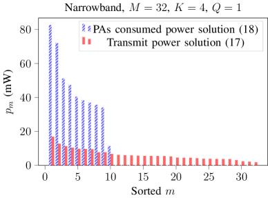
(a)

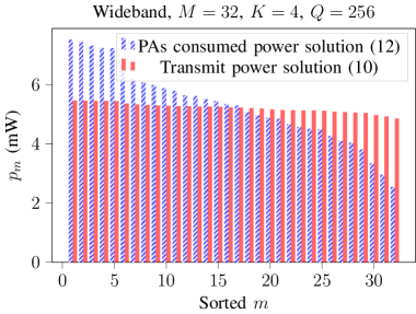
(b)

Figure 1: Transmit power as a function of the antenna index with decreasing allocated power, for $M=32$ antennas and $K=4$ users in i.i.d. Rayleigh fading. (a) Narrowband case, $Q=1$ subcarrier. The gain in PAs consumption is $1.19$, while the gain in BS consumption is $1.51$. (b) Wideband case, $Q=256$ subcarriers. The gains in PAs and BS consumption are both equal to $1.00$.

Fig. 1a shows the solutions, in terms of transmit powers at the different antennas, for the narrowband system and a specific channel realization, $K=4$ and $M=32$. As discussed in [28], the solution based on the PAs consumed power activates only few antennas, while the traditional ZF solution uses all the available antennas. Using (7) as a cost function induces sparsity in the power allocation. Note that, differently from the single-user case where only one antenna is used, the number of active antennas must be greater than $K$ to enable spatial multiplexing.

When moving to a wideband system, the precoder based on the PAs consumed power gradually uses more antennas as $Q$ increases. Fig. 1b shows the solutions for $Q=256$. The solution based on the PAs consumed power, although presenting more variability in the powers per antenna than the traditional solution, still activates all the BS antennas. Achieving the SINR constraints for all the subcarriers, while minimizing the consumed power by the PAs, requires using all the available antennas. In short, Fig. 1b shows that the per-subcarrier ZF (10) is efficient in terms of PAs consumed power.

VI-B Average Gains in Power Consumption

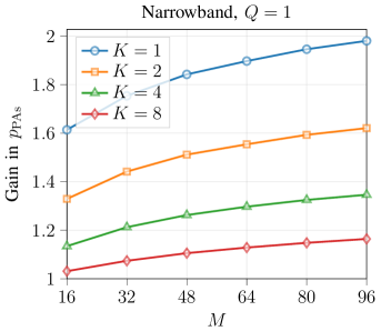
(a)

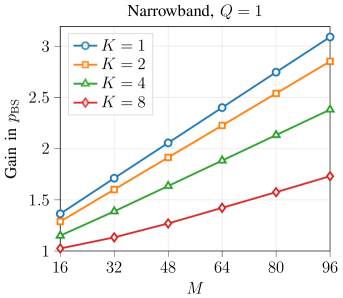
(b)

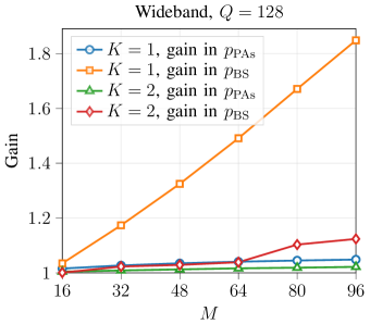
(c)

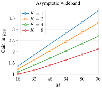
(d)

Figure 2: Gain in power consumption versus number of antennas for narrowband and wideband systems in i.i.d. Rayleigh fading ($2\cdot 10^{3}$ realizations), shown for different values of $K$. (a) Narrowband, gain in PAs consumption. (b) Narrowband, gain in BS consumption. (c) Wideband with $Q=128$, gain in PAs and BS consumption. (d) Asymptotic wideband, gain in asymptotic BS consumption. In this case, the gain is the BS consumption by activating $M$ antennas divided by the BS consumption by activating $M_{\mathrm{a}}^{\dagger}$ antennas.

Following the previous observations, Fig. 2a–2d show the relative differences in the consumed power for different systems. In the narrowband system and considering the PAs consumed power to evaluate the performance (Fig. 2a), the gain of the novel precoder (18) over the traditional one (17) is always greater than $1.5$ for $K=1$. When more users are present, the difference significantly decreases. For $K=8$, the ratio is below $1.2$ for every value of $M$. Instead, when the BS consumed power is evaluated, the achievable gains remain large even when more users are communicating (Fig. 2b). With $M=64$, the gain in the BS power consumption ranges from $1.4$ to $2.4$, depending on $K$.

In a wideband system with $Q=128$ subcarriers, the differences between the conventional and the novel precoder remain significant for $K=1$ and considering the BS consumption (Fig. 2c). However, the presence of $K=2$ users already requires the activation of all the antennas, and both the PAs and BS power consumption gains tend to $1$.

Considering the asymptotic wideband case, one can compute the gains achieved by using $M_{\mathrm{a}}^{\dagger}$ antennas over $M$. Fig. 2d shows that significant savings in BS consumption can be obtained, up to a factor of $3.8\times$. The benefits are similar to the ones achieved in a narrowband system when evaluating the BS consumption. For instance, when $K=4$ and $M=48$, the conventional precoder consumes $1.7$ times more power than the optimized precoder.

VI-C Asymptotic Wideband Regime

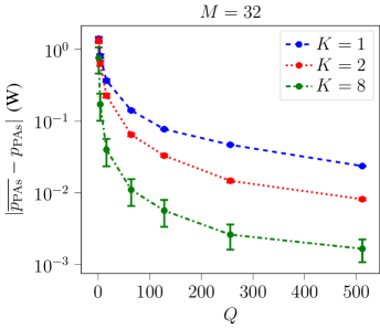
(a)

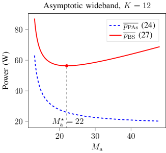
(b)

Figure 3: (a) Magnitude of the difference between the asymptotic and non-asymptotic PAs consumptions versus number of subcarriers for $M=32$ and different values of $K$. The non-asymptotic consumptions are computed through simulations, and the confidence intervals of the results are depicted, where the width is set to two times the variance of the results. The differences become smaller as $Q$ increases. (b) Asymptotic PAs and BS power consumption versus number of active antennas for $M=48$ and $K=12$. The number of antennas $M_{\mathrm{a}}^{\star}$ is also shown.

Fig. 3a illustrates the validity of the asymptotic results in Section V for $M=32$ and different values of $K$. The simulated PAs consumed powers converge to the asymptotic values, and $Q=128$ is already sufficient to allow the asymptotic result to be a tight approximation (i.e., the average errors are below $10^{-1}$). The trend of the asymptotic PAs and BS consumed powers as a function of $M_{\mathrm{a}}$ is shown in Fig. 3b, for $K=12$. The PAs consumed power decreases monotonically with $M_{\mathrm{a}}$, while the BS consumed power first decreases for small $M_{\mathrm{a}}$ (it is beneficial to use more antennas to reduce the PAs consumed power) and then increases for large $M_{\mathrm{a}}$ (it is detrimental to use more antennas due to the larger circuit power consumption). The convexity of (27) implies a global minimum.

The achievable power consumption savings by activating $M_{\mathrm{a}}^{\dagger}$ antennas can be also characterized as a function of the number of users. Fig. 4 illustrates the comparison for $M=64$. We consider the number of users to be an indication of the system traffic and load. Indeed, the per-antenna power constraints are not binding when $K$ is small, and they gradually start to be active when $K$ increases. The conventional precoder always utilizes all the $M$ antennas, while the optimized precoder adapts the number of utilized antennas to the traffic. The value of $M_{\mathrm{a}}^{\dagger}$ grows proportionally to $K$, as shown in Fig. 4b. When the system becomes more loaded, $M_{\mathrm{a}}^{\dagger}$ increases due to the larger value of $p_{\mathrm{PAs}}$ and due to the transmit power constraint (i.e., more antennas need to be saturated to achieve the QoS constraints). The BS consumptions by activating $M$ and $M_{\mathrm{a}}^{\dagger}$ antennas eventually converge (Fig. 4a). We also make a comparison with a precoder that always uses the minimum number of antennas ($K+1$). This precoder minimizes the BS consumption when $K=1$, and then starts to diverge from the optimal precoder because it does not counterbalance the increase in $p_{\mathrm{PAs}}$ with the utilization of more antennas.

In terms of achievable savings (i.e., the ratio between the asymptotic BS consumptions of the benchmark and optimized precoders), Fig. 4b shows that the optimized precoder reduces up to a factor of $2.8\times$ the consumption in low load with respect to the conventional precoder. When $K=10$, we can still achieve a gain equal to $1.5$. For more users, the gain reduces and eventually vanishes (all antennas are activated in both cases). The savings over the precoder that activates $K+1$ antennas follow the opposite trend, increasing in high load up to a factor of $2.2\times$.

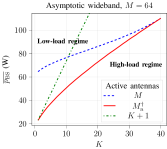
(a)

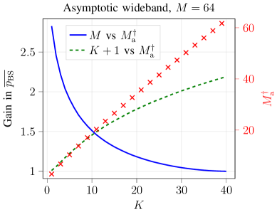
(b)

Figure 4: Characterization of the asymptotic wideband system as a function of $K$ for $M=64$, averaged over $2\cdot 10^{3}$ channel realizations. (a) Asymptotic BS power consumption (27) by using $M$, $K+1$, and $M_{\mathrm{a}}^{\dagger}$ antennas. (b) Referring to the same simulations, ratio between $\overline{p_{\mathrm{BS}}}$ by activating $M$ antennas and $\overline{p_{\mathrm{BS}}}$ by activating $M_{\mathrm{a}}^{\dagger}$ antennas (solid line), ratio between $\overline{p_{\mathrm{BS}}}$ by activating $K+1$ antennas and $\overline{p_{\mathrm{BS}}}$ by activating $M_{\mathrm{a}}^{\dagger}$ antennas (dashed line), and optimized number of active antennas $M_{\mathrm{a}}^{\dagger}$ (crosses).

VI-D Complexity Analysis

To quantify the computational complexity of the proposed precoders, we calculate the number of complex floating point operations (flops). As a reference for the number of flops required by standard linear algebraic operations, we consider [34, App. C.1.1].

VI-D1 Wideband System

In the wideband system, we need to calculate (12). The computation of both $\boldsymbol{\mathrm{H}}_{q}\boldsymbol{\mathrm{D}}_{\boldsymbol{\mathrm{p}}}^{1/2}$ and $\boldsymbol{\mathrm{D}}_{\boldsymbol{\mathrm{p}}}^{1/2}\boldsymbol{\mathrm{H}}_{q}^{\mathrm{H}}$ require $KM$ flops, corresponding to a scalar multiplication for each element of $\boldsymbol{\mathrm{H}}_{q}$. Computing $\boldsymbol{\mathrm{H}}_{q}\boldsymbol{\mathrm{D}}_{\boldsymbol{\mathrm{p}}}^{1/2}\boldsymbol{\mathrm{H}}_{q}^{\mathrm{H}}$, which is a symmetric matrix, requires $K^{2}M$ flops. Using Cholesky factorization and forward and backward substitution, we can compute the $m$-th row of the matrix $\boldsymbol{\mathrm{D}}_{\boldsymbol{\mathrm{p}}}^{1/2}\boldsymbol{\mathrm{H}}_{q}^{\mathrm{H}}\left(\boldsymbol{\mathrm{H}}_{q}\boldsymbol{\mathrm{D}}_{\boldsymbol{\mathrm{p}}}^{1/2}\boldsymbol{\mathrm{H}}_{q}^{\mathrm{H}}\right)^{-1}$ with $\frac{1}{3}K^{3}+2K^{2}$ flops. The forward and backward substitutions need to be performed $M$ times, therefore the number of flops becomes $\frac{1}{3}K^{3}+2K^{2}M$. At the end, the scaling by $\tilde{\boldsymbol{\mathrm{D}}}_{\boldsymbol{\mathrm{\gamma}}}^{1/2}\sigma_{\nu}$ requires $K$ flops. All that needs to be repeated for every subcarrier. By adding the terms, we obtain $\frac{1}{3}K^{3}Q+3K^{2}MQ+2KMQ+KQ$ flops, which scales as $\mathcal{O}\left(K^{3}Q+K^{2}MQ\right)$. Before computing (12), the powers at the antennas need to be retrieved. The computation of (13) requires, other than the necessary flops to compute $\boldsymbol{\mathrm{W}}_{q}$, $KQ$ multiplications to calculate the magnitudes and $K+Q-2$ additions to calculate the sums. Multiplying by $M$, we obtain $KQM+KM+QM-2M$ additional flops. The trend, however, remains $\mathcal{O}\left(K^{3}Q+K^{2}MQ\right)$. By using Algorithm 1, the computation of powers is repeated until convergence. If the algorithm converges in $I$ iterations, the total number of flops is $\mathcal{O}\left(K^{3}QI+K^{2}MQI\right)$. The conventional ZF, instead, requires $\mathcal{O}\left(K^{3}Q+K^{2}MQ\right)$ flops.

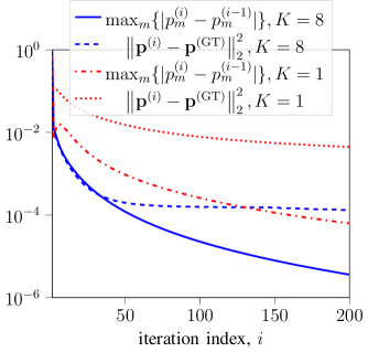
Figure 5: Performance of Algorithm 1 when $Q=1$ and $M=32$, using a tolerance $\varepsilon=10^{-4}$. The ground truth $\boldsymbol{\mathrm{p}}^{\mathrm{(GT)}}$ is computed with a convex solver. Results are averaged over $10^{3}$ executions of the algorithm.

TABLE II: Precoders complexity in the three analyzed systems.

System	Proposed sol.	Conventional sol.
Wideband	$\mathcal{O}\left(K^{3}QI+K^{2}MQI\right)$	$\mathcal{O}\left(K^{3}Q+K^{2}MQ\right)$
Narrowband	$\mathcal{O}\left(K^{3}I+K^{2}MI\right)$	$\mathcal{O}\left(K^{3}+K^{2}M\right)$
As. wideband	$\mathcal{O}\left(K^{3}Q+K^{2}M_{\mathrm{a}}Q\right)$	$\mathcal{O}\left(K^{3}Q+K^{2}MQ\right)$

Fig. 5 illustrates the convergence of the iterative algorithm. We show two narrowband cases because, when $Q$ increases, the convergence is faster (i.e., in tens of iterations), likely due to the more uniform power allocation that might be associated with fewer changes from one iteration to the other. We display the maximum absolute variation among the powers between iterations and the squared norm of the difference between the current solution and the ground truth, which is obtained through a convex solver. Given that the tolerance $\varepsilon$ is set to $10^{-4}$, the algorithm converges in $I\approx 200$ iterations for $K=1$, and in $I\approx 50$ iterations for $K=8$. Moreover, it can be seen as, considering this tolerance, the squared norm stays below $10^{-2}$.

VI-D2 Narrowband System

The same reasoning used for the wideband system applies to the narrowband one, which is then associated with a complexity of $\mathcal{O}\left(K^{3}I+K^{2}MI\right)$ flops for the PAs consumed power solution, while $\mathcal{O}\left(K^{3}+K^{2}M\right)$ for the transmit power solution.

VI-D3 Asymptotic Wideband System

In the asymptotic wideband scenario, the precoding matrices have $M_{\mathrm{a}}$ rows, then are computed with complexity $\mathcal{O}\left(K^{3}Q+K^{2}M_{\mathrm{a}}Q\right)$. Before executing Algorithm 2, which involves only comparisons, we need to solve the quartic equation (29). The solution of quartics can be computed with a fixed number of operations. Calculating the last coefficient in (29) requires the computation of $\mathrm{tr}\left(\boldsymbol{\mathrm{D}}_{\boldsymbol{\mathrm{\beta}}}^{-1}\boldsymbol{\mathrm{D}}_{\boldsymbol{\mathrm{\gamma}}}\right)$, which has complexity $\mathcal{O}\left(K\right)$. Therefore, we can consider that retrieving $M_{\mathrm{a}}^{\dagger}$, which needs to be recomputed when the large-scale fading coefficients change, has lower complexity than retrieving the precoding matrices, which instead need to be retrieved every time the small-scale fading coefficients change. We can therefore consider the complexity to be $\mathcal{O}\left(K^{3}Q+K^{2}M_{\mathrm{a}}Q\right)$. In the conventional case, the complexity remains $\mathcal{O}\left(K^{3}Q+K^{2}MQ\right)$.

Table II summarizes the complexities of the precoders for the three investigated systems. Given the behavior of Algorithm 1, the proposed wideband and narrowband precoders have complexities of $1$ or $2$ orders of magnitudes larger than the conventional precoders. However, the larger complexity is justified by the large savings shown in Fig. 2, especially for narrowband systems. Instead, the asymptotic wideband precoder has better performance and lower complexity in low-to-medium load.

VII Conclusion

In this paper, we have studied mMIMO precoders optimizing consumed power in both narrowband and wideband systems. In narrowband systems not subject to per-antenna power constraints, the optimal precoder activates few BS antennas, with consequent savings up to a factor of $3\times$ in the BS consumption by deactivating the RF chains of the non-active antennas. In wideband systems, more BS antennas are progressively activated as the number of subcarriers increases, hence no RF chains can be switched off. The asymptotic analysis of wideband systems subject to per-antenna power constraints reveals, however, how a simple optimization on the number of active antennas can lead to BS consumption savings up to a factor of $2.8\times$ in low-traffic scenarios. Complexity analysis suggests the viability of the proposed solutions, with the number of active antennas that is only computed when the large-scale fading changes.

A fundamental extension of this work is the analysis in the context of distributed mMIMO. The power consumption model and QoS constraints might be redefined, depending on the selected implementation. Relevant aspects to be included in the characterization of cellular systems are the impact of non-ideal channel estimation and the effect of PA non-linear distortions. The comparison with hybrid precoding architectures constitutes also an interesting future direction, as well as the consideration of correlation between BS antennas in the channel modeling.

Appendix A Proof of Theorem 1

The Lagrangian function of problem (11) under $\mathbf{(As1)}$, where the Lagrange multipliers are $\left\{\lambda_{k^{\prime},k,q}\in\mathbb{C}\right\}$ and the single element of $\tilde{\boldsymbol{\mathrm{D}}}_{\boldsymbol{\mathrm{\gamma}}}^{1/2}\sigma_{\nu}$ is $d_{k^{\prime},k}$, is

$$\mathcal{L}\left(w_{0,0,0},\dotsc,w_{M-1,K-1,Q-1},\lambda_{0,0,0},\dotsc,\lambda_{K-1,K-1,Q-1}\right)$$ (34)

$$=\underbrace{\sum_{m=0}^{M-1}\left(\sum_{k=0}^{K-1}\sum_{q=0}^{Q-1}|w_{m,k,q}|^{2}\right)^{1/2}}_{(a)}+\underbrace{\sum_{q=0}^{Q-1}\Re\left(\sum_{k^{\prime}=0}^{K-1}\sum_{k=0}^{K-1}\lambda_{k^{\prime},k,q}\right.\left.\left(\sum_{m=0}^{M-1}h_{k^{\prime},m,q}w_{m,k,q}-d_{k^{\prime},k}\right)\right)}_{(b)}.$$

By using the property that, for $z\in\mathbb{C}$, $\Re\{{z}\}=\frac{1}{2}\left(z+z^{*}\right)$, we expand the constraint as

$$(b) =\frac{1}{2}\sum_{q=0}^{Q-1}\sum_{k^{\prime}=0}^{K-1}\sum_{k=0}^{K-1}\lambda_{k^{\prime},k,q}\left(\sum_{m=0}^{M-1}h_{k^{\prime},m,q}w_{m,k,q}-d_{k^{\prime},k}\right)$$ (35)

$$+\frac{1}{2}\sum_{q=0}^{Q-1}\sum_{k^{\prime}=0}^{K-1}\sum_{k=0}^{K-1}\lambda_{k^{\prime},k,q}^{*}\left(\sum_{m=0}^{M-1}h_{k^{\prime},m,q}^{*}w_{m,k,q}^{*}-d_{k^{\prime},k}\right).$$

Let us now compute the Wirtinger derivative of the Lagrangian function using the properties that, for $z\in\mathbb{C}$, $\frac{\partial z^{*}}{\partial z^{*}}=1$, $\frac{\partial\left(zz^{*}\right)}{\partial z^{*}}=z$, and $\frac{\partial z}{\partial z^{*}}=0$ [35]. To differentiate $(a)$, we note that, for $z_{1},\dotsc,z_{N}\in\mathbb{C}$, $\frac{\partial}{\partial z_{n}^{*}}\left(\left(\sum_{n=1}^{N}z_{n}z_{n}^{*}\right)^{1/2}\right)=\frac{1}{2}z_{n}\left(\sum_{n^{\prime}=1}^{N}z_{n^{\prime}}z_{n^{\prime}}^{*}\right)^{-1/2}$. The differentiation of $(b)$ follows from the basic properties listed above. The Wirtinger derivative of $\mathcal{L}$ with respect to a precoding coefficient is then given by

$$\frac{\partial\mathcal{L}}{\partial w_{m,k,q}^{*}}=\frac{1}{2}\frac{w_{m,k,q}}{\left(\sum_{k^{\prime}=0}^{K-1}\sum_{q^{\prime}=0}^{Q-1}|w_{m,k^{\prime},q^{\prime}}|^{2}\right)^{1/2}}+\frac{1}{2}\sum_{k^{\prime}=0}^{K-1}\lambda_{k^{\prime},k,q}^{*}h_{k^{\prime},m,q}^{*}.$$ (36)

Recalling that $p_{m}=\sum_{k=0}^{K-1}\sum_{q=0}^{Q-1}|w_{m,k,q}|^{2}$ and setting (36) to zero, we obtain

$$\frac{\partial\mathcal{L}}{\partial w_{m,k,q}^{*}}=0\iff w_{m,k,q}=-p_{m}^{1/2}\sum_{k^{\prime}=0}^{K-1}\lambda_{k^{\prime},k,q}^{*}h_{k^{\prime},m,q}^{*}.$$ (37)

The constraint gives

$$\sum_{m=0}^{M-1}h_{k^{\prime},m,q}^{*}w_{m,k,q}^{*}-d_{k^{\prime},k}=0$$ (38)

which, using (37), can be rewritten as

$$\sum_{m=0}^{M-1}h_{k^{\prime},m,q}^{*}p_{m}^{1/2}\sum_{k^{\prime\prime}=0}^{K-1}\lambda_{k^{\prime\prime},k,q}h_{k^{\prime\prime},m,q}=-d_{k^{\prime},k}.$$ (39)

We are left with the following system of equations

$$\begin{cases}w_{m,k,q}=-p_{m}^{1/2}\displaystyle\sum_{k^{\prime}=0}^{K-1}\lambda_{k^{\prime},k,q}^{*}h_{k^{\prime},m,q}^{*}\\ \displaystyle\sum_{m=0}^{M-1}h_{k^{\prime},m,q}^{*}p_{m}^{1/2}\displaystyle\sum_{k^{\prime\prime}=0}^{K-1}\lambda_{k^{\prime\prime},k,q}h_{k^{\prime\prime},m,q}=-d_{k^{\prime},k}\end{cases}.$$ (40)

Making use of $\boldsymbol{\mathrm{D}}_{\boldsymbol{\mathrm{p}}}=\mathrm{diag}\left(p_{0},\dotsc,p_{M-1}\right)$ and denoting with $\boldsymbol{\mathrm{\Lambda}}_{q}\in\mathbb{C}^{K\times K}$ the matrix containing the Lagrange multipliers for the subcarrier $q$, (40) can be written in matrix form as

$$\begin{cases}\boldsymbol{\mathrm{W}}_{q}=-\boldsymbol{\mathrm{D}}_{\boldsymbol{\mathrm{p}}}^{1/2}\boldsymbol{\mathrm{H}}_{q}^{\mathrm{H}}\boldsymbol{\mathrm{\Lambda}}_{q}^{*}\\ \boldsymbol{\mathrm{H}}_{q}^{*}{\boldsymbol{\mathrm{D}}_{\boldsymbol{\mathrm{p}}}^{1/2}}\boldsymbol{\mathrm{H}}_{q}^{\mathrm{T}}\boldsymbol{\mathrm{\Lambda}}_{q}=-\tilde{\boldsymbol{\mathrm{D}}}_{\boldsymbol{\mathrm{\gamma}}}^{1/2}\sigma_{\nu}\end{cases}.$$ (41)

The matrix $\boldsymbol{\mathrm{\Lambda}}_{q}$ is then given by

$$\boldsymbol{\mathrm{\Lambda}}_{q}=-\left(\boldsymbol{\mathrm{H}}_{q}^{*}{\boldsymbol{\mathrm{D}}_{\boldsymbol{\mathrm{p}}}^{1/2}}\boldsymbol{\mathrm{H}}_{q}^{\mathrm{T}}\right)^{-1}\tilde{\boldsymbol{\mathrm{D}}}_{\boldsymbol{\mathrm{\gamma}}}^{1/2}\sigma_{\nu}$$ (42)

therefore, by substituting it back to the first expression of (41), we obtain

$$\boldsymbol{\mathrm{W}}_{q}=\boldsymbol{\mathrm{D}}_{\boldsymbol{\mathrm{p}}}^{1/2}\boldsymbol{\mathrm{H}}_{q}^{\mathrm{H}}\left(\boldsymbol{\mathrm{H}}_{q}\boldsymbol{\mathrm{D}}_{\boldsymbol{\mathrm{p}}}^{1/2}\boldsymbol{\mathrm{H}}^{\mathrm{H}}_{q}\right)^{-1}\tilde{\boldsymbol{\mathrm{D}}}_{\boldsymbol{\mathrm{\gamma}}}^{1/2}\sigma_{\nu}.$$ (43)

Appendix B Proof of Theorem 2

Problem (11) is convex. In the asymptotic wideband regime, the power allocations in the neighborhood of the global optimum achieve substantially the same performance. Fig. 1b illustrates as (i) different power allocations consume approximately the same amount of power while achieving the users’ QoS, and (ii) the power tends to be uniformly allocated among the antennas as $Q$ increases. Among the possible allocations, let us consider a uniform allocation, i.e., $\boldsymbol{\mathrm{D}}_{\boldsymbol{\mathrm{p}}}=p\boldsymbol{\mathrm{I}}_{M}$. When validating the asymptotic results, we will prove that this allocation is optimal. Equation (13) becomes

$$p=\sum_{q=0}^{Q-1}\sum_{k=0}^{K-1}\left|\left[\boldsymbol{\mathrm{H}}_{q}^{\mathrm{H}}\left(\boldsymbol{\mathrm{H}}_{q}\boldsymbol{\mathrm{H}}_{q}^{\mathrm{H}}\right)^{-1}\tilde{\boldsymbol{\mathrm{D}}}_{\boldsymbol{\mathrm{\gamma}}}^{1/2}\sigma_{\nu}\right]_{m,k}\right|^{2}.$$ (44)

By summing over the antennas we can write

$$\begin{split}Mp&=\sum_{q=0}^{Q-1}\sum_{m=0}^{M-1}\sum_{k=0}^{K-1}\left|\left[\boldsymbol{\mathrm{H}}_{q}^{\mathrm{H}}\left(\boldsymbol{\mathrm{H}}_{q}\boldsymbol{\mathrm{H}}_{q}^{\mathrm{H}}\right)^{-1}\tilde{\boldsymbol{\mathrm{D}}}_{\boldsymbol{\mathrm{\gamma}}}^{1/2}\sigma_{\nu}\right]_{m,k}\right|^{2}\\ &=\sum_{q=0}^{Q-1}\mathrm{tr}\left(\boldsymbol{\mathrm{H}}_{q}^{\mathrm{H}}\left(\boldsymbol{\mathrm{H}}_{q}\boldsymbol{\mathrm{H}}_{q}^{\mathrm{H}}\right)^{-1}\tilde{\boldsymbol{\mathrm{D}}}_{\boldsymbol{\mathrm{\gamma}}}\sigma_{\nu}^{2}\left(\boldsymbol{\mathrm{H}}_{q}\boldsymbol{\mathrm{H}}_{q}^{\mathrm{H}}\right)^{-1}\boldsymbol{\mathrm{H}}_{q}\right).\end{split}$$ (45)

By using the cyclic property of the trace

$$p=\frac{1}{M}\sum_{q=0}^{Q-1}\mathrm{tr}\left(\left(\boldsymbol{\mathrm{H}}_{q}\boldsymbol{\mathrm{H}}_{q}^{\mathrm{H}}\right)^{-1}\tilde{\boldsymbol{\mathrm{D}}}_{\boldsymbol{\mathrm{\gamma}}}\sigma_{\nu}^{2}\right).$$ (46)

Under $\mathbf{(As2)}$ and recalling that $\tilde{\boldsymbol{\mathrm{D}}}_{\boldsymbol{\mathrm{\gamma}}}=\frac{1}{Q}\boldsymbol{\mathrm{D}}_{\boldsymbol{\mathrm{\gamma}}}$, the law of large numbers gives

$$\frac{1}{Q}\sum_{q=0}^{Q-1}\left(\boldsymbol{\mathrm{H}}_{q}\boldsymbol{\mathrm{H}}_{q}^{\mathrm{H}}\right)^{-1}\boldsymbol{\mathrm{D}}_{\boldsymbol{\mathrm{\gamma}}}\sigma_{\nu}^{2}\to\mathbb{E}\left\{\left(\boldsymbol{\mathrm{H}}_{q}\boldsymbol{\mathrm{H}}_{q}^{\mathrm{H}}\right)^{-1}\boldsymbol{\mathrm{D}}_{\boldsymbol{\mathrm{\gamma}}}\sigma_{\nu}^{2}\right\}$$ (47)

then (46) becomes

$$p\to\frac{1}{M}\mathrm{tr}\left(\mathbb{E}\left\{\left(\boldsymbol{\mathrm{H}}_{q}\boldsymbol{\mathrm{H}}_{q}^{\mathrm{H}}\right)^{-1}\boldsymbol{\mathrm{D}}_{\boldsymbol{\mathrm{\gamma}}}\sigma_{\nu}^{2}\right\}\right).$$ (48)

Under $\mathbf{(As3)}$, the Gram matrix $\boldsymbol{\mathrm{H}}_{q}\boldsymbol{\mathrm{H}}_{q}^{\mathrm{H}}\sim\mathcal{C}\mathcal{W}\left(\boldsymbol{\mathrm{D}}_{\boldsymbol{\mathrm{\beta}}},M,K\right)$, then its inverse $\left(\boldsymbol{\mathrm{H}}_{q}\boldsymbol{\mathrm{H}}_{q}^{\mathrm{H}}\right)^{-1}\sim{\mathcal{C}\mathcal{W}}^{-1}\left(\boldsymbol{\mathrm{D}}_{\boldsymbol{\mathrm{\beta}}}^{-1},M,K\right)$ [36]. We obtain a deterministic expression of the transmit power at each antenna

$$p\to\frac{1}{M(M-K)}\mathrm{tr}\left(\boldsymbol{\mathrm{D}}_{\boldsymbol{\mathrm{\beta}}}^{-1}\boldsymbol{\mathrm{D}}_{\boldsymbol{\mathrm{\gamma}}}\sigma_{\nu}^{2}\right)$$ (49)

thereby the total PAs consumed power can be computed as

$$p_{\mathrm{PAs}}=M\alpha p^{1/2}\to\alpha\left(\frac{M}{M-K}\mathrm{tr}\left(\boldsymbol{\mathrm{D}}_{\boldsymbol{\mathrm{\beta}}}^{-1}\boldsymbol{\mathrm{D}}_{\boldsymbol{\mathrm{\gamma}}}\sigma_{\nu}^{2}\right)\right)^{1/2}.$$ (50)

Appendix C Proof of Lemma 1

The optimal number of active antennas lies in between $K+1$ (required by the ZF constraint) and $M$. By considering a continuous number of active antennas $x\in\mathbb{R}$, the function (27)

$$f(x)=t\left(\frac{x}{x-K}\right)^{1/2}+p_{\mathrm{fix}}+\mathcal{C}x$$ (51)

where $t=\alpha\left(\mathrm{tr}\left(\boldsymbol{\mathrm{D}}_{\boldsymbol{\mathrm{\beta}}}^{-1}\boldsymbol{\mathrm{D}}_{\boldsymbol{\mathrm{\gamma}}}\sigma_{\nu}^{2}\right)\right)^{1/2}$, is convex in the domain $]K,M]$. To prove that, let us compute the first derivative of $f$

$$\frac{df(x)}{dx}=t\left(\frac{x^{-1/2}}{2\left(x-K\right)^{1/2}}-\frac{x^{1/2}}{2\left(x-K\right)^{3/2}}\right)+\mathcal{C}=-\frac{t}{2}\left(\frac{Kx^{-1/2}}{\left(x-K\right)^{3/2}}\right)+\mathcal{C}.$$ (52)

By taking the second derivative

$$\frac{d^{2}f(x)}{dx^{2}}=-\frac{tK}{2}\left(-\frac{x^{-3/2}}{2\left(x-K\right)^{3/2}}-\frac{3x^{-1/2}}{2\left(x-K\right)^{5/2}}\right)=\frac{tK}{4}\frac{4x-K}{x^{3/2}\left(x-K\right)^{5/2}}$$ (53)

we can see that, for $x>K$, (53) is always positive. To minimize (51), one can compute its derivative with respect to $x$, given in (52), set it to zero, and isolate the constant term, obtaining the following polynomial

$$x\left(x-K\right)^{3}-\frac{tK}{2\mathcal{C}}=0.$$ (54)

From Descartes’ rule of signs, (54) has 2 positive real roots. Among them, there is only one bigger than $K$. This can also be seen by visualizing (27) in Fig. 3b. The $\min\{\cdot\}$ and $\max\{\cdot\}$ operations guarantee that the final value stays within the allowed range. Due to the convexity of the function (51), the result of the ceil-floor operation $\left\lfloor\cdot\right\rceil$ is guaranteed to be the optimal integer value.

Appendix D Proof of Theorem 3

Let us consider problem (26). Fixing the value of $M_{\mathrm{a}}$, the minimization problem with respect to the precoding coefficients is

$$\operatorname*{minimize}_{\begin{subarray}{c}\{w_{m,k,q}\}\\ m=0,\dotsc,M_{\mathrm{a}}-1\end{subarray}}\quad\quad p_{\mathrm{BS}}=p_{\mathrm{PAs}}+p_{\mathrm{fix}}+\mathcal{C}M_{\mathrm{a}}$$ (55a)

$$\mathrm{\;\;subject\ to}\quad\quad \boldsymbol{\mathrm{H}}_{q}\boldsymbol{\mathrm{W}}_{q}=\tilde{\boldsymbol{\mathrm{D}}}_{\boldsymbol{\mathrm{\gamma}}}^{1/2}\sigma_{\nu}\;\;\forall q,$$ (55b)

$$p_{m}\leq p_{\mathrm{max}}\;\;\forall m.$$ (55c)

From Theorem 2, we know that the solution to the above problem (in the asymptotic wideband regime and i.i.d. Rayleigh fading) when the per-antenna power constraints are not binding tends to allocate the power uniformly among the antennas,

$$p_{m}\to\overline{p}=\frac{1}{M_{\mathrm{a}}(M_{\mathrm{a}}-K)}\mathrm{tr}\left(\boldsymbol{\mathrm{D}}_{\boldsymbol{\mathrm{\beta}}}^{-1}\boldsymbol{\mathrm{D}}_{\boldsymbol{\mathrm{\gamma}}}\sigma_{\nu}^{2}\right)\quad\forall m.$$ (56)

Let us consider two cases, recalling that we are considering an arbitrary value of $M_{\mathrm{a}}$:

1. $\overline{p}\leq p_{\mathrm{max}}$, which guarantees that the above solution is optimal. Indeed, solution (56) minimizes (55a) while satistying (55b), and in this case it fulfils also (55c).

2. $\overline{p}>p_{\mathrm{max}}$, which indicates that the above solution is not feasible by using $M_{\mathrm{a}}$ antennas. Indeed, to satisfy the constraints (55c), we would need to decrease every value of $p_{m}$ to $p_{\mathrm{max}}$ or a smaller quantity. By doing this, we would need a solution consuming less power (given that PAs consumption increases monotonically with $p_{m}$) while fulfilling (55b). This is not possible, otherwise this new solution would correspond to the optimal one for the unconstrained problem, i.e., the one allocating the power $\overline{p}$ to all antennas.

The above reasoning entails that, in the asymptotic wideband regime and i.i.d. Rayleigh fading, the per-antenna power constraints imply a lower bound on the number of active antennas $M_{\mathrm{a}}$ (by using (56) and assuming $M_{\mathrm{a}}>K$)

$$\overline{p}\leq p_{\mathrm{max}}\iff M_{\mathrm{a}}^{2}-KM_{\mathrm{a}}-\frac{\mathrm{tr}\left(\boldsymbol{\mathrm{D}}_{\boldsymbol{\mathrm{\beta}}}^{-1}\boldsymbol{\mathrm{D}}_{\boldsymbol{\mathrm{\gamma}}}\sigma_{\nu}^{2}\right)}{p_{\mathrm{max}}}\geq 0,$$ (57)

$$M_{\mathrm{a}}\geq\frac{1}{2}\left(K+\left(K^{2}+\frac{4\mathrm{tr}\left(\boldsymbol{\mathrm{D}}_{\boldsymbol{\mathrm{\beta}}}^{-1}\boldsymbol{\mathrm{D}}_{\boldsymbol{\mathrm{\gamma}}}\sigma_{\nu}^{2}\right)}{p_{\mathrm{max}}}\right)^{1/2}\right).$$ (58)

Using this lower bound as a constraint in the original problem, we can drop the per-antenna power constraints and solve the equivalent problem

$$\operatorname*{minimize}_{M_{a}}\quad \overline{p_{\mathrm{BS}}}=\alpha\left(\frac{M_{a}}{M_{a}-K}\mathrm{tr}\left(\boldsymbol{\mathrm{D}}_{\boldsymbol{\mathrm{\beta}}}^{-1}\boldsymbol{\mathrm{D}}_{\boldsymbol{\mathrm{\gamma}}}\sigma_{\nu}^{2}\right)\right)^{1/2}+p_{\mathrm{fix}}+\mathcal{C}M_{a}$$ (59)

$$\mathrm{subject\ to}\quad M_{a}\geq\frac{1}{2}\left(K+\left(K^{2}+\frac{4\mathrm{tr}\left(\boldsymbol{\mathrm{D}}_{\boldsymbol{\mathrm{\beta}}}^{-1}\boldsymbol{\mathrm{D}}_{\boldsymbol{\mathrm{\gamma}}}\sigma_{\nu}^{2}\right)}{p_{\mathrm{max}}}\right)^{1/2}\right),$$

$$M_{a}\leq M.$$

The condition in $\mathbf{(As4)}$ ensures that the power constraint is always satisfied by activating all the $M$ antennas. It can be simply derived from (56) by setting $M_{\mathrm{a}}=M$.

References

- [1] European Commission, “The European Green Deal,” COM (2019), p. 640, Nov. 2019.
- [2] International Telecommunication Union, “ITU-T L.1470 (01/2020): Greenhouse gas emissions trajectories for the information and communication technology sector compatible with the UNFCCC Paris Agreement,” 2020.
- [3] C. Andersson, J. Bengtsson, G. Byström, P. Frenger, Y. Jading, and M. Nordenström, “Improving energy performance in 5G networks and beyond,” Ericsson Technol. Rev., vol. 2022, no. 8, pp. 2–11, 2022.
- [4] C. Han et al., “Green radio: Radio techniques to enable energy-efficient wireless networks,” IEEE Commun. Mag., vol. 49, no. 6, pp. 46–54, 2011.
- [5] S. Buzzi, C.-L. I, T. E. Klein, H. V. Poor, C. Yang, and A. Zappone, “A survey of energy-efficient techniques for 5G networks and challenges ahead,” IEEE J. Sel. Areas Commun., vol. 34, no. 4, pp. 697–709, 2016.
- [6] D. López-Pérez et al., “A survey on 5G radio access network energy efficiency: Massive MIMO, lean carrier design, sleep modes, and machine learning,” IEEE Commun. Surveys Tuts., vol. 24, no. 1, pp. 653–697, 2022.
- [7] Huawei, “Green 5G white paper: Building green networks to lighten up the way to a low-carbon future,” Tech. Rep., Oct. 2021.
- [8] L. Golard, J. Louveaux, and D. Bol, “Evaluation and projection of 4G and 5G RAN energy footprints: the case of Belgium for 2020–2025,” Ann. Telecommun., Nov. 2022.
- [9] 3GPP, “3rd Generation Partnership Project; Technical Specification Group Radio Access Network; Study on network energy savings for NR (Release 18),” Tech. Rep. 38.864, Dec. 2022, version 18.0.0.
- [10] G. Auer et al., “How much energy is needed to run a wireless network?” IEEE Wireless Commun., vol. 18, no. 5, pp. 40–49, 2011.
- [11] X. Ge, J. Yang, H. Gharavi, and Y. Sun, “Energy efficiency challenges of 5G small cell networks,” IEEE Commun. Mag., vol. 55, no. 5, pp. 184–191, 2017.
- [12] S. Muneer, L. Liu, O. Edfors, H. Sjöland, and L. Van der Perre, “Handling PA nonlinearity in massive MIMO: What are the tradeoffs between system capacity and power consumption,” in Proc. Asilomar Conf. Signals Syst. Comput., 2020, pp. 974–978.
- [13] E. Björnson, M. Bengtsson, and B. Ottersten, “Optimal multiuser transmit beamforming: A difficult problem with a simple solution structure [lecture notes],” IEEE Signal Process. Mag., vol. 31, no. 4, pp. 142–148, 2014.
- [14] A. Grebennikov, RF and Microwave Power Amplifier Design, 1st ed. New York, NY, USA: McGraw-Hill, 2005.
- [15] Y. Chen, S. Zhang, S. Xu, and G. Y. Li, “Fundamental trade-offs on green wireless networks,” IEEE Commun. Mag., vol. 49, no. 6, pp. 30–37, 2011.
- [16] A. He et al., “Power consumption minimization for MIMO systems — A cognitive radio approach,” IEEE J. Sel. Areas Commun., vol. 29, no. 2, pp. 469–479, 2011.
- [17] 3.4 - 3.6 GHz, 3 Watt, 28 Volt GaN Power Amplifier Module, Qorvo, QPA3503, 2018, Rev. B.
- [18] D. Persson, T. Eriksson, and E. G. Larsson, “Amplifier-aware multiple-input multiple-output power allocation,” IEEE Commun. Lett., vol. 17, no. 6, pp. 1112–1115, 2013.
- [19] ——, “Amplifier-aware multiple-input single-output capacity,” IEEE Trans. Commun., vol. 62, no. 3, pp. 913–919, 2014.
- [20] H. V. Cheng, D. Persson, and E. G. Larsson, “Optimal MIMO precoding under a constraint on the amplifier power consumption,” IEEE Trans. Commun., vol. 67, no. 1, pp. 218–229, 2019.
- [21] H. V. Cheng, D. Persson, E. Björnson, and E. G. Larsson, “Massive MIMO at night: On the operation of massive MIMO in low traffic scenarios,” in Proc. IEEE Int. Conf. Commun., 2015, pp. 1697–1702.
- [22] E. Björnson, J. Hoydis, and L. Sanguinetti, “Massive MIMO networks: Spectral, energy, and hardware efficiency,” Found. Trends Signal Process., vol. 11, no. 3-4, pp. 154–655, 2017.
- [23] K. Senel, E. Björnson, and E. G. Larsson, “Joint transmit and circuit power minimization in massive MIMO with downlink SINR constraints: When to turn on massive MIMO?” IEEE Trans. Wireless Commun., vol. 18, no. 3, pp. 1834–1846, 2019.
- [24] J. Xu and L. Qiu, “Energy efficiency optimization for MIMO broadcast channels,” IEEE Trans. Wireless Commun., vol. 12, no. 2, pp. 690–701, 2013.
- [25] E. Björnson, L. Sanguinetti, J. Hoydis, and M. Debbah, “Optimal design of energy-efficient multi-user MIMO systems: Is massive MIMO the answer?” IEEE Trans. Wireless Commun., vol. 14, no. 6, pp. 3059–3075, 2015.
- [26] Y. Dong, Y. Huang, and L. Qiu, “Energy-efficient sparse beamforming for multiuser MIMO systems with nonideal power amplifiers,” IEEE Trans. Veh. Technol., vol. 66, no. 1, pp. 134–145, 2017.
- [27] M. M. A. Hossain, C. Cavdar, E. Björnson, and R. Jäntti, “Energy saving game for massive MIMO: Coping with daily load variation,” IEEE Trans. Veh. Technol., vol. 67, no. 3, pp. 2301–2313, 2018.
- [28] E. Peschiera and F. Rottenberg, “Linear precoder design in massive MIMO under realistic power amplifier consumption constraint,” in Proc. WIC/IEEE Symp. Inf. Theory Signal Process. Benelux, 2022.
- [29] E. Dahlman, S. Parkvall, and J. Sköld, 5G NR: The Next Generation Wireless Access Technology, 2nd ed. New York, NY, USA: Academic, 2020.
- [30] F. Rottenberg, G. Callebaut, and L. Van der Perre, “The Z3RO family of precoders cancelling nonlinear power amplification distortion in large array systems,” IEEE Trans. Wireless Commun., vol. 22, no. 3, pp. 2036–2047, 2023.
- [31] X. Gao, L. Dai, S. Han, C.-L. I, and R. W. Heath, “Energy-efficient hybrid analog and digital precoding for mmWave MIMO systems with large antenna arrays,” IEEE J. Sel. Areas Commun., vol. 34, no. 4, pp. 998–1009, 2016.
- [32] Q. Spencer, A. Swindlehurst, and M. Haardt, “Zero-forcing methods for downlink spatial multiplexing in multiuser MIMO channels,” IEEE Trans. Signal Process., vol. 52, no. 2, pp. 461–471, 2004.
- [33] S. Shmakov, “A universal method of solving quartic equations,” Int. J. Pure Appl. Math., vol. 2, no. 71, pp. 251–259, 2011.
- [34] S. Boyd and L. Vandenberghe, Convex Optimization. Cambridge, U.K.: Cambridge Univ. Press, 2004.
- [35] A. Hjørungnes, Complex-Valued Matrix Derivatives: With Applications in Signal Processing and Communications. Cambridge, U.K.: Cambridge Univ. Press, 2011.
- [36] D. Maiwald and D. Kraus, “On moments of complex Wishart and complex inverse Wishart distributed matrices,” in Proc. IEEE Int. Conf. Acoust., Speech Signal Process., vol. 5, 1997, pp. 3817–3820.