Exact enumeration of fullerenes

Abstract.

A fullerene, or buckyball, is a trivalent graph on the sphere with only pentagonal and hexagonal faces. Building on ideas of Thurston, we use modular forms to give an exact formula for the number of oriented fullerenes with a given number of vertices.

1. Introduction

We call a triangulation $\mathcal{T}$ of $S^{2}$ convex if every vertex has valence $6$ or less. The curvature of a vertex $v_{i}\in\mathcal{T}$ is $\kappa_{i}:=6-{\rm valence}(v_{i})$ and the curvature profile $\{\kappa_{1},\dots,\kappa_{m}\}$ is the multiset of nonzero curvatures. It is a consequence of Euler’s formula that $\sum\kappa_{i}=12$ and so there are at most $12$ vertices of positive curvature. We call the dual complex of a triangulation with exactly $12$ vertices of positive curvature a buckyball or fullerene—a trivalent graph on the sphere, whose faces are all pentagons and hexagons.

The terminology originates from the famous Buckminsterfullerene molecule, with chemical formula ${\rm C}_{60}$. It is formed from $60$ carbon atoms, each one bonded to three other carbon atoms in $sp^{2}$-hybridized orbitals, and forming a spherical molecule with carbon rings of length $5$ and $6$, see Figure 1. The molecule was first discovered in the laboratory in 1985 by Kroto, Heath, O’Brien, Curl, and Smalley [13], work which received the 1996 Nobel prize in chemistry.

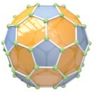
Figure 1. The Buckminsterfullerene molecule

1.1. Algorithmic enumeration

Soon after the discovery of fullerenes, the question of their enumeration was explored by chemists, computer scientists, and mathematicians, resulting in a large body of literature: see Liu, Klein, Schmalz, and Seitz [15], Manolopoulos and May [19], Manolopoulos and Fowler [17, 18], Sah [20], Yoshida and Osawa [28], Brinkmann and Dress [3], Hasheminezhad, Fleischner, and McKay [12], Brinkmann, Goedgebeur, and McKay [4, 11].

The earliest algorithms, proposed by Manolopoulos et al. enumerated fullerenes by spiraling outward from a face, as one might peel an orange. A spiral representation $[i_{1},\dots,i_{12}]$ of the fullerene is then simply the list of $12$ indices corresponding to positions of the 12 pentagons in a face spiral of the given fullerene. The canonical spiral representation is the lexicographically minimal spiral representation. For example, the canonical spiral representation of Buckminsterfullerene is

$$[1,7,9,11,13,15,18,20,22,24,26,32].$$

Remarkably, there are fullerenes with no spiral representation, the first counterexample being an isomer of ${\rm C}_{380}$ with tetrahedral symmetry [5].

The spiral algorithm was supplanted by Brinkmann and Dress’s algorithm, implemented in the program fullgen. It generates all fullerenes with a given number of vertices by stitching together patches which are bounded by zigzag (Petrie) paths. This was again supplanted by buckygen, developed by Brinkmann, Goedgebeur, and McKay [4]. It generates larger fullerenes from smaller ones, by excising a patch of faces and replacing it with a larger patch having the same boundary. There are three irreducible fullerenes in the buckygen algorithm, isomers of ${\rm C}_{20}$, ${\rm C}_{28}$, and ${\rm C}_{30}$.

Because of its recursion, buckygen is much more efficient than fullgen, especially for generating fullerenes up to $n$ vertices. Contradicting results of buckygen and fullgen led to the detection of a small programming error in fullgen, which led to a discrepancy in the counts beyond $136$ vertices. After this was fixed, the two programs agreed up to 380 vertices, giving a high degree of confidence in their accuracy.

The input to this paper was generated with buckygen, see Appendix A by Jan Goedgebeur, with a built-in setting that counts enantiomorphic (mirror) fullerenes as distinct. This makes the mathematical enumeration somewhat less complicated; we hope to return to the case of enumerating unoriented fullerenes in future work.

1.2. Mathematical enumeration

Thurston’s paper “Shapes of Polyhedra” [27] introduced the moduli spaces $\mathcal{M}_{\alpha_{1}\,,\,\dots\,,\,\alpha_{k}}$ of flat cone spheres (modulo scaling): These are flat metrics on $S^{2}$ with $k$ conical singularities $p_{i}$ of cone angles $2\pi-\alpha_{i}$ and $\alpha_{i}\in(0,2\pi)$. The Gauss-Bonnet formula implies $\sum\alpha_{i}=4\pi$. Alexandrov’s theorem [1] states that a flat cone sphere is isometric to a convex polyhedron in $\mathbb{R}^{3}$, unique up to rigid motion.

Thurston proved that $\mathcal{M}_{\alpha_{1}\,,\,\dots\,,\,\alpha_{k}}$ admits a canonical Hermitian metric, endowing it with the structure of a locally symmetric space: It admits a local isometry [27, Thm. 0.2] to complex hyperbolic space

$$\mathbb{CH}^{k-3}:=\mathbb{P}\{v\in\mathbb{C}^{1,{k-2}}\,\big{|}\,v\cdot v>0\},$$

also called the complex ball. The metric completion $\overline{\mathcal{M}}_{\alpha_{1}\,,\,\dots\,,\,\alpha_{k}}$ is a complex hyperbolic cone manifold, and admits a moduli-theoretic interpretation, corresponding to allowing collections of cone points $\{p_{i}\,\big{|}\,i\in I\}$ to coalesce, so long as $\sum_{i\in I}\alpha_{i}<2\pi$.

The completed Thurston moduli space of interest to this paper is

$$M:=\overline{\mathcal{M}}_{\pi/3\,,\,\dots\,,\,\pi/3}$$

as every convex triangulation defines a point in it, by declaring each triangle metrically equilateral of side length $1$. A convex triangulation corresponds to a fullerene if and only if the corresponding flat cone sphere has $12$ distinct points of positive curvature, or equivalently, defines a point in the open stratum $\mathcal{M}_{\pi/3\,,\,\dots\,,\,\pi/3}$. There are $48$ possible curvature profiles for convex triangulations of the two sphere $S^{2}$, in bijection with the $48$ partitions $\{\kappa_{1},\dots,\kappa_{m}\}$ of $12$ into parts of size $5$ or less. Each such partition corresponds to a curvature stratum:

$$M=\overline{\mathcal{M}}_{\pi/3\,,\,\dots\,,\,\pi/3}=\!\!\!\!\!\!\coprod_{\begin{subarray}{c}\sum\kappa_{i}=12\\ \kappa_{i}\in\{1,2,3,4,5\}\end{subarray}}\!\!\!\!\!\!\mathcal{M}_{\kappa_{1}\pi/3\,,\,\dots\,,\,\kappa_{m}\pi/3}.$$

Thurston proved that $M=\mathbb{P}\Gamma\backslash\mathbb{CH}^{9}$ is a global ball quotient for an arithmetic subgroup $\Gamma\subset U(1,9)$; it is the largest-dimensional completed Thurston moduli space which is a global quotient. See also [22].

Definition 1.1.

An Eisenstein lattice $\Lambda$ is a finitely generated $\mathbb{Z}[\zeta_{6}]$-module $\Lambda\simeq\mathbb{Z}[\zeta_{6}]^{k}$, together with a non-degenerate $\mathbb{Z}[\zeta_{6}]$-valued Hermitian inner product $v\star w$. Its signature $(m,n)$ is the signature of $\Lambda\otimes_{\mathbb{Z}[\zeta_{6}]}\mathbb{C}\simeq\mathbb{C}^{m,n}$.

Theorem 1.2 ([27, Thm. 0.1]).

There is an Eisenstein lattice $\Lambda$ of signature $(1,9)$ for which convex triangulations of the sphere, up to oriented isomorphism, are in bijection with $\Gamma\backslash\Lambda^{+}$. Here $\Lambda^{+}\subset\Lambda$ is the set of vectors of positive norm and $\Gamma=U(\Lambda)$ is the group of unitary isometries.

Furthermore, for a vector $v\in\Lambda^{+}$ corresponding to a triangulation, the number of triangles is $\tfrac{2}{3}(v\star v)$.

The point in $\mathbb{P}\Gamma\backslash\mathbb{CH}^{9}=M$ corresponding to the triangulation is the $\Gamma$-orbit of the complex line $\mathbb{C}v\in\mathbb{CH}^{9}$.

Thurston’s theorem bounds the growth rate for the number of fullerenes with $2n$ vertices as $O(n^{9})$. The computational chemists were aware of this fact and Thurston’s result, see for instance the survey of Schwerdtfeger, Wirz, and Avery [23].

In 2017, the authors used Thurston’s theorem to enumerate convex triangulations, when counted with an appropriate weight:

Definition 1.3.

Define the mass of a convex triangulation to be

$$m(\mathcal{T}):=\frac{1}{|{\rm Aut}^{+}(\mathcal{T})|}\prod_{i=1}^{m}\frac{(1-\kappa_{i}/6)^{\kappa_{i}-1}}{\kappa_{i}!}$$

where $\kappa_{i}$ are the curvatures and ${\rm Aut}^{+}(\mathcal{T})$ is the group of oriented automorphisms. Alternatively, we can define $m(\mathcal{T})={|{\rm Stab}_{\Gamma}(v)|}^{-1}$ where $v\in\Lambda^{+}$ corresponds to $\mathcal{T}$.

Theorem 1.4 ([10, Thm. 1.1]).

The mass-weighted sum of all convex triangulations with $2n$ triangles is exactly

$$\sum_{|\mathcal{T}|=2n}m(\mathcal{T})=\frac{809}{2^{15}3^{13}5^{2}}\sum_{d\mid n}d^{9}.$$

The key point of the proof is to use the Siegel theta correspondence to show that the mass-weighted generating function $f(q)$ for convex triangulations is a modular form of weight $10$ for $SL_{2}(\mathbb{Z})$. Up to a constant scaling factor, this pins down $F(q)$ uniquely as the Eisenstein series $E_{10}(q)=-\frac{1}{264}+\sum_{n\geq 1}\big{(}\sum_{d\mid n}d^{9}\big{)}q^{n}$. To determine the constant, it suffices to compute the the weighted count of triangulations with $2$ triangles.

Let $G$ be a group acting on a set $S$, with finitely many orbits $\{G\cdot s\,\big{|}\,s\in S\}$, and finite stabilizers. It is most natural to weight the count of orbits by $|{\rm Stab}_{G}(s)|^{-1}$ where $s\in S$ is an orbit representative. This way, passing to a finite index subgroup $H\subset G$ changes the weighted count by the index $[G:H]$. It is this manner of enumeration employed in Theorem 1.4, with $G=U(\Lambda)$ and $S=\Lambda^{+}$.

1.3. Main results

The enumeration of fullerenes by chemists is not a mass-weighted count. In contrast to the mass-weighted enumeration, we call an unweighted count of orbits naive enumeration.

Definition 1.5.

Let ${\rm BB}(q):=\sum_{n\geq 1}{\rm BB}_{n}q^{n}$ where ${\rm BB}_{n}$ is the naive count of oriented fullerenes with $2n$ vertices. We have

$${\rm BB}(q)=q^{10}+q^{12}+q^{13}+3q^{14}+3q^{15}+10q^{16}+9q^{17}+23q^{18}+\cdots.$$

Obviously, ${\rm BB}(q)\in\mathbb{Z}[[q]]$ has integer coefficients, while the weighted generating function for convex triangulations $F(q)\in\mathbb{Q}[[q]]$ does not. Even though the $q^{n}$-coefficients of $F(q)$ and ${\rm BB}(q)$ as asymptotic to each other as $n\to\infty$, the series differ in two key ways:

1. Counts for $F(q)$ are over the completed space $M=\overline{\mathcal{M}}_{\pi/3\,,\,\dots\,,\,\pi/3}$ whereas counts for ${\rm BB}(q)$ are over the open stratum $\mathcal{M}_{\pi/3\,,\,\dots\,,\,\pi/3}$.

2. Counts for $F(q)$ are weighted, but counts for ${\rm BB}(q)$ are naive. Both $\{\kappa_{1},\dots,\kappa_{m}\}$ and ${\rm Aut}^{+}(\mathcal{T})$ affect the weight.

Our goal is to surmount these obstacles, and count fullerenes naively. While conceptually simpler, this is mathematically much more complicated.

The main idea is to prove that for each curvature profile and automorphism group, there is an appropriately weighted count of such triangulations which is again a (quasi)modular form, but of lower weight and higher level. Then, by Möbius inversion on strata, the naive count ${\rm BB}(q)$ has an expression as a weighted inclusion-exclusion of weighted counts. So ${\rm BB}(q)$ is a linear combination of modular forms, but of mixed levels and weights. Sah [21, Thm. 3.4] was the first to realize ${\rm BB}_{n}$ would have a formula of an arithmetic nature.

Our formula is proven by bounding the levels and weights of these modular forms explicitly, and using the buckygen program as input—we solve a large linear system for the coefficients of the linear combination. Fortuitously, buckygen can compute $200$ Fourier coefficients ${\rm BB}_{n}$. This exceeds the $152$-dimensional space of modular forms in which we prove ${\rm BB}(q)$ lives. Once a formula in a finite-dimensional space is established, the ambient space of modular forms is pruned, resulting in our main theorem:

Theorem 1.6.

${\rm BB}(q)$ is an explicit linear combination of Eisenstein series, of weight at most $10$ and levels lying in $\{1,2,3,4,5,6,9,12,15,18\}.$

More precise statements are given in the body of the paper, see Theorem 3.25. Using this explicit formula, we can compute the number of oriented fullerenes far beyond buckygen. In fact, evaluating the formula is computationally only as hard as factoring $n$.

2. Strata of triangulations

We must understand the stratification of $M=\overline{\mathcal{M}}_{\pi/3\,,\,\dots\,,\,\pi/3}=\mathbb{P}\Gamma\backslash\mathbb{CH}^{9}$ by curvatures and automorphism groups in more detail.

Definition 2.1.

The automorphism stratification of $M$ is the stratification by oriented automorphism groups ${\rm Aut}^{+}(\mathcal{T})$. Let $M_{G}\subset M$ denote the stratum of flat cone spheres with ${\rm Aut}^{+}(\mathcal{T})=G$. So $M=\coprod_{G}M_{G}$.

A flat cone sphere can be specified by a Lauricella differential, i.e. a multivalued differential $\omega$ on $\mathbb{P}^{1}$ with fractional pole orders (see [7, 16]). Such a differential defines a flat structure $\mathcal{T}$ on $\mathbb{P}^{1}\simeq S^{2}$ by declaring $z$ a local flat coordinate if $dz=\omega$, i.e. the flat metric is $|\omega|^{2}$. Two Lauricella differentials $\omega_{1}$ and $\omega_{2}$ determine the same flat cone sphere, mod scaling, if and only if $\omega_{1}=c\omega_{2}$ for $c\in\mathbb{C}^{*}$. Conversely, every flat cone sphere is naturally a Riemann surface isomorphic to $\mathbb{P}^{1}$, and defines a Lauricella differential by declaring $\omega=dz$ for a local flat coordinate $z$.

Given any 12 points $p_{i}\in\mathbb{P}^{1}$, no more than 5 of which are simultaneously equal, and any constant $c\in\mathbb{C}^{*}$, we form the Lauricella differential

(1) $$\omega=c(x-p_{1})^{-1/6}\cdots(x-p_{k})^{-1/6}\,dx$$

in which the product is over $p_{i}\neq\infty$. Then the resulting flat cone sphere lies in $M$, and conversely every point of $M$ can be described by a Lauricella differential of this form with $c=1$. Thus, $M$ also admits a description as the space of $12$ unordered points on $\mathbb{P}^{1}$, in which up to $5$ points can coalesce, up to the action of the holomorphic automorphism group of $\mathbb{P}^{1}$.

Note that such a differential $\omega$ is multivalued and that $\omega=\zeta\omega$ for $\zeta$ any sixth root of unity.

Proposition 2.2.

The possible automorphism groups ${\rm Aut}^{+}(\mathcal{T})$ for some $\mathcal{T}\in M$ are precisely:

1. a cyclic group $C_{n}$ for $n\in\{1,2,3,4,5,6,7,8,9,10,11\}$,

2. a dihedral group $D_{n}$ for $n\in\{2,3,4,5,6,8,10,12\}$, or

3. one of the three exceptional groups $T$, $O$, $I$, which are respectively symmetries of the tetrahedron, octahedron, icosahedron.

Proof.

The three exceptional groups are realized by putting $p_{1},\dots,p_{12}$ at the vertices of the tetrahedron, octahedron, and dodecahedron respectively. Note that for $T$, three points coincide at each vertex, and for $O$, two points coincide at each vertex.

The remaining finite subgroups of $PGL_{2}(\mathbb{C})$ are $C_{n}$ and $D_{n}$. The orbits of the $C_{n}$ action, acting by $x\mapsto\zeta_{n}x$, are the singleton poles $\{0\}$, $\{\infty\}$ and free orbits of size $n$. Since no more than $5$ points can coalesce at $0$ or $\infty$, there must be at least one free orbit and so $n\leq 12$. If $n=12$, then the points $p_{i}$ lie in a single free orbit of $C_{12}$, in which case $D_{12}$ symmetry is automatic. For $C_{n}$ with $n\leq 11$, we can always put some points $p_{i}$ at the poles $0$, $\infty$ with non-equal weights less than $6$, and add a union of free orbits, to get a flat cone sphere $\mathcal{T}\in M$ with cyclic $C_{n}$ symmetry.

To realize $D_{n}$ symmetry with $n\in\{2,3,4,5,6\}$, we place $6-n$ points at each of $0$, $\infty$ and place the remaining $2n$ points on a free $D_{n}$ orbit. To realize $D_{n}$ symmetry with $n\in\{8,10,12\}$, we place $\frac{12-n}{2}$ points at each of $0$, $\infty$ and put the remaining $n$ points along the equator in a $D_{n}$ orbit of size $n$. The other dihedral groups $D_{n}$ for $n\in\{7,9,11,13,14,\dots\}$ are not realizable because either they contain $C_{n}$ with $n\geq 13$ or the weights at $0$, $\infty$ cannot be made equal for parity reasons. ∎

Not all automorphism groups of flat cone spheres in $M$ are realized as automorphism groups of triangulations:

Example 2.3.

The cyclic group $C_{11}$ acts on $\mathbb{P}^{1}$ by rotations, with a generator acting by $x\mapsto\zeta_{11}x$. There is a flat cone sphere with one point at $\infty$ and $11$ points on the equator, all of curvature $1$, associated to the Lauricella differential $(1-x^{11})^{-1/6}\,dx$. This flat cone sphere is not realized by an equilateral triangulation.

If $\omega$ is a Lauricella differential of the form $\eqref{eqn:lauricella}$, then the integral of $\omega$ along any path is well-defined up to a sixth root of unity. By the periods of $\omega$, we mean the integrals along paths between singular points, considered as numbers in $\mathbb{C}/\langle\zeta_{6}\rangle$. It follows from [27] that:

Proposition 2.4.

Equilaterally triangulated flat cone spheres are equivalent to Lauricella differentials of the form (1), all of whose periods lie in $\mathbb{Z}[\zeta_{6}]$.

Proof.

If $\mathcal{T}$ is triangulated, we choose the Lauricella differential $\omega$ so that the period map sends any given triangle of $\mathcal{T}$ onto a triangle of the standard triangulation of $\mathbb{C}$. (Recall that $\omega$ is a priori determined only up to a complex number of norm one). Then the developing map sends all singularities of $\mathcal{T}$ onto points of $\mathbb{Z}[\zeta_{6}]$, i.e. the periods of $\omega$ will lie in $\mathbb{Z}[\zeta_{6}]$.

In the other direction, if all the periods of $\omega$ lie in $\mathbb{Z}[\zeta_{6}]$, then we recover the triangulation by declaring a point $p\in\mathcal{T}$ to be a vertex if the integral of $\omega$ from any singularity to $p$ lies in $\mathbb{Z}[\zeta_{6}]$, and a path from one vertex to another to be an edge if the integral of $\omega$ along that path takes values between 0 and 1, up to the indeterminacy of $\langle\zeta_{6}\rangle$. ∎

Proposition 2.5.

Suppose that a flat cone sphere $\mathcal{T}$ admits an equilateral triangulation. Then ${\rm Aut}^{+}(\mathcal{T})$ preserves the triangulation.

Proof.

Let $\omega=c\prod_{i}(x-p_{i})^{-1/6}\,dx$ be the Lauricella differential associated to the triangulation. Oriented automorphisms of $\mathcal{T}$ are exactly given by $g\in PGL_{2}(\mathbb{C})$ for which $g^{*}\omega\in\mathbb{C}\omega$ or equivalently $g^{*}\{p_{i}\}=\{p_{i}\}$. Since $\gamma$ has finite order, we necessarily have $g^{*}\omega=\zeta\omega$ for some root of unity $\zeta$, well-defined up to a sixth root of unity. When $\mathcal{T}$ is triangulated, then $g$ preserves the triangulation iff $\zeta=1$ (up to a sixth root of unity).

Let $\gamma$ be any path between singularities of $\mathcal{T}$ with nonzero period. Since

$$\int_{g^{*}\gamma}\omega=\int_{\gamma}g^{*}\omega=\zeta\int_{\gamma}\omega$$

and all periods of $\omega$ are in $\mathbb{Z}[\zeta_{6}]$, we see that $\zeta\in\mathbb{Q}[\zeta_{6}]$. But the only roots of unity in $\mathbb{Q}[\zeta_{6}]$ are sixth roots of unity, so $g$ must preserve the Lauricella differential, and hence the triangulation. ∎

If $\mathcal{T}$ is a flat cone sphere, and $G\subset\mathrm{Aut}^{+}(\mathcal{T})$, then the quotient can also be given the structure of a flat cone sphere, where the cone angle at a point in the quotient is the cone angle upstairs divided by the size of its stabilizer. However, we will also find it useful to consider the quotient as an orbifold. To that end, we define:

Definition 2.6.

A flat cone orbifold is a flat metric on $S^{2}$ with $k$ conical singularities of cone angle $2\pi-\alpha_{i}$ and specified “ramification orders” $n_{i}$ subject to the condition that $n_{i}(2\pi-\alpha_{i})\in(0,2\pi]$ and $\alpha_{i}>0$.

A local orbifold chart near such a cone point is given by an $n_{i}$-to-$1$ branched cover from a cone of angle $n_{i}(2\pi-\alpha_{i})$, which is a local isometry away from the branch point.

Definition 2.7.

An orbitriangulation of a flat cone orbifold is a system of compatible equilateral triangulations in every possible orbifold chart.

For the orbifold $\mathcal{T}/G$, an orbitriangulation of $\mathcal{T}/G$ is the same thing as a $G$-invariant triangulation of $\mathcal{T}$. By Proposition 2.5, every triangulation of $\mathcal{T}$ is $G$-invariant, so in particular we have

Corollary 2.8.

The quotient of a triangulated flat cone sphere in $\mathcal{T}\in M$ by a subgroup of its automorphism group ${\rm Aut}^{+}(\mathcal{T})$ is an orbitriangulated flat cone sphere in $M$.

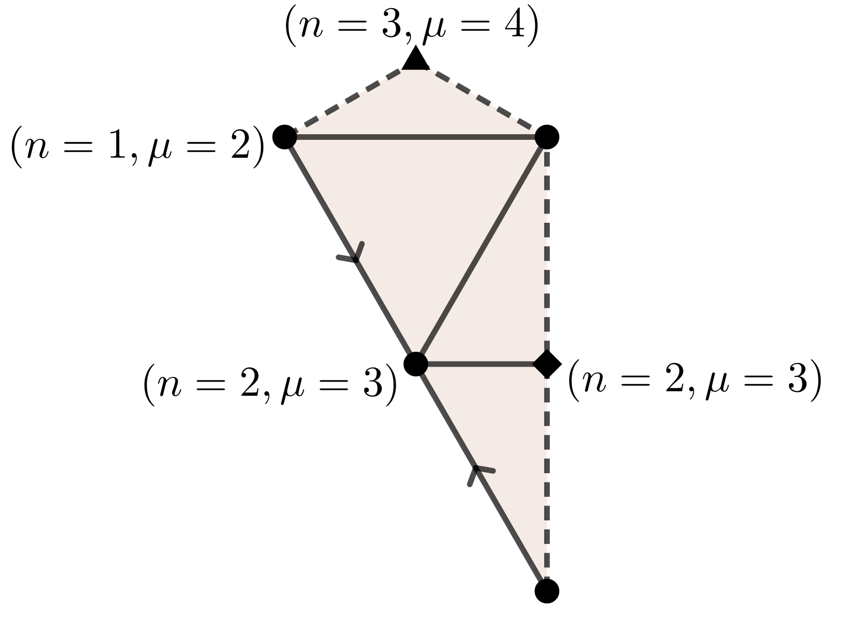
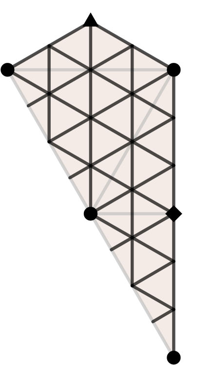
Figure 2. An orbitriangulation (left) and a triangulation of the underlying flat cone sphere.

Example 2.9.

Figure 2 (left) shows an orbitriangulation. The points are labeled with their ramification orders $n$ and their curvature $\mu$, which is related to the cone angle deficit $\alpha$ by $\alpha/(2\pi)=\mu/6$. The unlabeled vertices are identified with the $(n=1,\mu=2)$ vertex by the gluing, which identifies the dotted lines in pairs and the solid lines as marked. As required, we have $n(6-\mu)\leq 6$ at each point.

Since the orbifold indices are $(3,2,2)$, this is equal to $\mathbb{P}^{1}/D_{3}$ as an orbifold. The corresponding $D_{3}$-invariant triangulation upstairs has $6$ singular points $p_{i}$ each of curvature $\kappa_{i}=2$, the preimages of the $(n=1,\mu=2)$ point. In this example, none of the orbifold points are singular upstairs.

Remark 2.10.

A flat cone orbifold is not necessarily the quotient of a manifold (i.e. a good orbifold). For example, in the same picture of Figure 2, if we had declared the vertex between the two arrows to instead be $(n=1,\mu=3)$, this would be an orbitriangulated flat cone orbifold that is not good. By the convexity inequality, every good flat cone orbifold is the quotient either of the plane (if $n_{i}(2\pi-\alpha_{i})=2\pi$ for all $i$) or of a flat cone sphere.

Note that an orbitriangulated flat cone sphere also admits a triangulation, but by triangles of side length $\tfrac{1}{2\sqrt{3}}$ rather than $1$. See Figure 2 (right).

Remark 2.11.

As we can see from Example 2.3, if $\mathcal{T}$ is not triangulated, then its quotient by its automorphism group may not even lie in $M$. For example, the quotient by the $C_{11}$ action on the flat cone sphere $(1-x^{11})^{-1/6}\,dx$ lies in $\mathcal{M}_{61\pi/33\,,\,20\pi/11\,,\,\pi/3}$.

Proposition 2.12.

The poset diagram of automorphism groups of convex triangulations is:

Proof.

We first observe that any element $g\in{\rm Aut}^{+}(\mathcal{T})$ has order at most $6$. This is because any $g\in PGL_{2}(\mathbb{C})$ fixes some point $p$. Assuming $g\neq 1$, either $p$ is the center of a triangular face and ${\rm ord}(g)=3$, or $p$ is the center of an edge and ${\rm ord}(g)=2$, or $p$ is a vertex and ${\rm ord}(g)$ divides ${\rm val}(p)\leq 6.$

Conversely, we can easily construct convex triangulations on which $C_{n}$ and $D_{n}$ act for $n\leq 6$, for instance $n$-gonal bipyramids, and there are triangulated platonic solids with automorphism groups $T$, $O$, $I$.

But, note that $C_{4}$, $C_{5}$, $C_{6}$ do not appear in the diagram. The reason is the following: Any cyclic symmetry of order $4$, $5$, $6$ must fix a vertex of the triangulation of valence $4$, $5$, $6$, at both of the poles of the cyclic rotation. There are either one or two remaining free $C_{4}$, $C_{5}$, $C_{6}$ orbits. Thus $C_{4}$, $C_{5}$, $C_{6}$ symmetry always implies $D_{4}$, $D_{5}$, $D_{6}$ symmetry—there is always an involution switching the two poles and the remaining free orbit(s). ∎

We now analyze how automorphism groups and curvatures interact.

Definition 2.13.

The bistratification of $M=\mathbb{P}\Gamma\backslash\mathbb{CH}^{9}$ is the stratification by conjugacy classes of inertia groups ${\rm Stab}_{\mathbb{P}\Gamma}(p)$ where $p\in\mathbb{CH}^{9}$.

Proposition 2.14.

The bistrata are the intersections of automorphism strata and curvature strata.

Proof.

The local stabilizer of some $[\mathcal{T}]\in M$ corresponding to $\mathbb{C}v\in\mathbb{CH}^{9}$ has a canonical extension structure

$$0\to\textstyle\prod_{i}B_{\kappa_{i}}\to{\rm Stab}_{\mathbb{P}\Gamma}(\mathbb{C}v)\to{\rm Aut}^{+}(\mathcal{T})\to 0$$

where $B_{\kappa_{i}}$ is the image in $U(\Lambda)$ of the local braid group of the $\kappa_{i}$ colliding singularities. Thus, ${\rm Stab}_{\mathbb{P}\Gamma}(p)$ jumps in size exactly when (1) singularities further collide or (2) the size of the automorphism group increases.∎

A bistratum of $M$ is specified by the list of pairs $\{(n_{i},\mu_{i})\}$ of ramification orders and curvatures, at each of the singularities of the quotient flat cone orbifold. Such a list determines a nonempty bistratum if and only if

1. The multiset of ramification orders $\{n_{i}\}$ not equal to 1 are those of a good orbifold $\mathbb{P}^{1}/G$, for one of the groups $G$ in Proposition 2.12,

2. for each $i$, $0<\mu_{i}<6$ and $n_{i}(6-\mu_{i})\leq 6$, and

3. $\sum_{i}\mu_{i}=12$.

The automorphism group $G$ of the corresponding bistratum is determined by the $\{n_{i}\}$. The curvature profile $\{\kappa_{j}\}$ of the flat cone sphere upstairs is determined as follows: Each singular point of the quotient orbifold with indices $(n_{i},\mu_{i})$ satisfying $n_{i}(6-\mu_{i})<6$ corresponds to $|G|/n_{i}$ singular points upstairs, each with curvature $\kappa_{j}$ given by the formula

$$6-\kappa_{j}=n_{i}(6-\mu_{i}).$$

The singular points of the quotient orbifold with $n_{i}(6-\mu_{i})=6$ are non-singular upstairs.

Notation 2.15.

We introduce an alternative notation for the bistratum $\{(n_{i},\mu_{i})\}$. First, instead of listing the ramification orders $\{n_{i}\}$, we write the corresponding group $G$. Second, we order the $\mu_{i}$ so that they correspond to the ramification orders of $\mathbb{P}^{1}/G$ in descending order. Third, we add a superscript $\bf e$ to the index $\mu_{i}=3$ whenever $n_{i}=2$, and we add a superscript $\bf f$ to the index $\mu_{i}=4$ whenever $n_{i}=3$.

So, for example, the bistratum $\{(3,4),(2,3),(2,3),(1,2)\}$ of the orbifold depicted in Figure 2 is written $(D_{3},\{4^{\bf f},3^{\bf e},3^{\bf e},2\})$. We will call the list $\{\mu_{i}\}$ with superscripts a decorated curvature profile.

The explanation for the superscripts is the following. The superscript $\bf f$ stands for face, because a singular point of an orbifold with $\mu_{i}=4$ and $n_{i}=3$ may lie in the middle of a face of the orbitriangulation. The superscript $\bf e$ stands for edge, because a point of the orbifold with $\mu_{i}=3$ and $n_{i}=2$ may lie in the middle of an edge of the orbitriangulation. Of course, both points may also lie at a vertex.

On the other hand, a singular point without a superscript must lie at a vertex. This is because first, the only possible non-vertex points in a triangulation, with non-trivial stabilizers under an automorphism group, are the center of an edge and the center of a face, with stabilizers of size $2$ and $3$ respectively. So $n$ must be $2$ or $3$. Second, if $n(6-\mu)\neq 6$, the point upstairs has positive curvature and hence must be a vertex.

Thus, the justification for this alternative notation is that the orbitriangulations in a given stratum of flat cone orbifolds depend only on the decorated curvature profile—that is, which $\mu_{i}$ are decorated with an ${\bf f}$ or ${\bf e}$, see Proposition 2.17 for a more precise statement.

Definition 2.16.

The undecorated profile $\mu^{u}$ of a quotient profile $\mu$ is the result of deleting the decorations ${\bf f}$, ${\bf e}$.

Undecorating corresponds to forgetting the orbifold structure, i.e. taking the coarse space or resetting $n_{i}=1$. The orbitriangulations with curvature profile $\mu^{u}$ are simply triangulations in the curvature stratum $\mu^{u}$.

Proposition 2.17.

Let $\kappa$ be an (undecorated) curvature profile. There is a Hermitian Eisenstein sublattice $\Lambda_{\kappa}\subset\Lambda$ of signature $(1,{\rm len}(\kappa)-3)$ and a subgroup $\Gamma_{\kappa}\subset{\rm Stab}_{\Gamma}(\Lambda_{\kappa})$ for which $\Gamma_{\kappa}\backslash\Lambda_{\kappa}^{+}$ is in bijection with convex triangulations of the sphere, whose curvature profile is a collision of $\kappa$.

Now let $\mu$ be a decorated curvature profile and let $\mu^{u}$ be is undecoration. There is an Eisenstein module

$$\Lambda_{\mu^{u}}\subset\Lambda_{\mu}\subset\tfrac{1}{2(1+\zeta_{6})}\Lambda_{\mu^{u}}$$

of signature $(1,{\rm len}(\mu)-3)$ and a subgroup $\Gamma_{\mu}\subset{\rm Stab}_{\Gamma}(\Lambda_{\mu})$ for which $\Gamma_{\mu}\backslash\Lambda_{\mu}^{+}$ is in bijection with orbitriangulations with profile a collision of $\mu$.

Proof.

First, we treat the undecorated case. In the local period coordinates $(\int_{p_{j}}^{p_{j+1}}\omega)\in\mathbb{C}^{1,9}$, the condition that $\kappa_{i}$ singularities $p_{1},\dots,p_{\kappa_{i}}$ have coalesced is locally described by the equation

$$\textstyle\int_{p_{j}}^{p_{j+1}}\omega=0\textrm{ for }j=1,\dots,\kappa_{i}-1.$$

This is a $\mathbb{Z}[\zeta_{6}]$-linear condition, and thus cuts out a sublattice $\Lambda_{\kappa_{i}}\subset\Lambda$ exactly corresponding to triangulations with a point of curvature $\kappa_{i}$. These linear conditions can be imposed for each coalescence, and are independent, giving a sublattice

$$\Lambda_{\kappa}:=\cap_{i}\,\Lambda_{\kappa_{i}}\subset\Lambda.$$

In fact, it is shown in Thurston’s paper that the completed moduli space $\overline{\mathcal{M}}_{\kappa_{1}\pi/3\,,\,\dots\,,\,\kappa_{m}\pi/3}$ is a subball quotient $\mathbb{P}\Gamma_{\kappa}\backslash\mathbb{CH}^{{\rm len}(\kappa)-3}\subset\mathbb{P}\Gamma\backslash\mathbb{CH}^{9}$. The bijection between $\Gamma_{\kappa}\backslash\Lambda^{+}_{\kappa}$ and triangulations works in the same way as for $M$: the triangulation associated to $v\in\Lambda_{\kappa}^{+}$ corresponds to

$$\mathbb{C}v\in\mathbb{P}\{x\in\Lambda_{\kappa}\otimes_{\mathbb{Z}[\zeta_{6}]}\mathbb{C},\big{|}\,x\star x>0\}=\mathbb{CH}^{{\rm len}(\kappa)-3}.$$

We now consider the decorated case $\mu$. The moduli space of flat cone orbifolds containing orbitriangulations with curvature profile a collision of $\mu$ is simply $\overline{\mathcal{M}}_{\mu_{1}\pi/3\,,\,\dots\,,\,\mu_{r}\pi/3}$ as in the undecorated case. Triangulations with curvature profile $\mu^{u}$ correspond to $\Gamma_{\mu^{u}}$ orbits of $v\in\Lambda_{\mu^{u}}^{+}$ by the previous paragraph. In period coordinates, admitting a triangulation is simply the condition $\int_{p_{j}}^{p_{j+1}}\omega\in\mathbb{Z}[\zeta_{6}]\textrm{ for all }j$.

Let $\mu_{i}$ be an undecorated curvature. Admitting an orbitriangulation amounts to the slightly weaker period conditions:

(2) $$\begin{aligned} \textstyle\int_{p_{i}}^{p_{j}}\omega&\in\tfrac{1}{1+\zeta_{6}}\mathbb{Z}[\zeta_{6}]\textrm{ if }\mu_{j}=4^{\bf f},\\ \textstyle\int_{p_{i}}^{p_{j}}\omega&\in\tfrac{1}{2}\mathbb{Z}[\zeta_{6}]\textrm{ if }\mu_{j}=3^{\bf e},\\ \textstyle\int_{p_{i}}^{p_{j}}\omega&\in\mathbb{Z}[\zeta_{6}]\textrm{ otherwise.}\end{aligned}$$

This is because $\frac{1}{1+\zeta_{6}}\mathbb{Z}[\zeta_{6}]$ is the superlattice of $\mathbb{Z}[\zeta_{6}]$ containing the centers of the standard triangular tiles of $\mathbb{C}$ (and the vertices), while $\frac{1}{2}\mathbb{Z}[\zeta_{6}]$ is the superlattice of $\mathbb{Z}[\zeta_{6}]$ containing the centers of the edges (and the vertices).

Conditions (2) on period integrals describe a finite index enlargement $\Lambda_{\mu}\supset\Lambda_{\mu^{u}}$ which is contained in $\frac{1}{2(1+\zeta_{6})}\Lambda_{\mu^{u}}$. Equality of orbitriangulations is the same as equality of the underlying flat cone spheres, preserving the ramification orders $n_{i}$. Thus, $\Gamma_{\mu}\subset\Gamma_{\mu^{u}}$ is a finite index subgroup. ∎

Remark 2.18.

We will identify properties of the Eisenstein lattices/modules $\Lambda_{\kappa}$ and $\Lambda_{\mu}$ in greater detail in the following section.

We call $\Lambda_{\mu}$ an Eisenstein module, rather than an Eisenstein lattice, for the following reason: Its natural Hermitian inner product $\star$ need not be valued in $\mathbb{Z}[\zeta_{6}]$. Unlike $\Lambda_{\mu^{u}}$, there may be vectors $v\in\Lambda_{\mu}$ for which $v\star v\notin 3\mathbb{Z}$, because an orbitriangulation need not have an even integer number of triangles.

Definition 2.19.

Let $f_{\mu}(q)=c_{0}+\sum_{n>0}c_{n}q^{n}$, where $n\in\tfrac{1}{6}\mathbb{Z}$, be the completed generating function for orbitriangulations in the decorated stratum $\mu$: Concretely, for $n>0$, $c_{n}$ is the count of orbitriangulations $v\in\Gamma_{\mu}\backslash\Lambda_{\mu}^{+}$ with $2n$ triangles, weighted by $|{\rm Stab}_{\Gamma_{\mu}}(v)|^{-1}$.

We define the constant term $c_{0}$ in the next section.

Example 2.20.

We define the important generating function

$$A(q):=\tfrac{1}{6}\sum_{v\in\mathbb{Z}[\zeta_{6}]}q^{v\overline{v}}.$$

For any $0$-dimensional decorated profile (i.e. ${\rm len}(\mu)=3$), we have that $f_{\mu}(q)=A(q^{r})$ where $r\in\tfrac{1}{6}\mathbb{Z}$ is the (possibly fractional) number of triangles in the smallest area orbitriangulation $\mathcal{T}_{0}$. This is because every orbitriangulation with decorated profile $\mu$ is the result of scaling $\mathcal{T}_{0}$ the flat structure by some nonzero Eisenstein integer.

Definition 2.21.

Let ${\rm BB}_{(G,\mu)}(q)$ to be generating function for naive enumeration of triangulations in the bistratum $(G,\mu)$ i.e. triangulations with automorphism group $G$ and decorated quotient profile $\mu$.

Note that here we are counting the upstairs triangulations, not the quotient orbitriangulations, so ${\rm BB}_{(G,\mu)}(q)\in\mathbb{Z}[[q]]$.

Proposition 2.22.

Let $\{M_{(H,\nu)}\}$ be the collection of all lower-dimensional bistrata in the closure $\overline{M}_{(G,\mu)}$ of a fixed bistratum. There exist constants $c_{(H,\nu)}\in\mathbb{Q}$ and $c_{0}\in\mathbb{R}$ for which

$$f_{\mu}(q^{|G|})={\rm BB}_{(G,\mu)}(q)+c_{0}+\sum_{(H,\nu)}c_{(H,\nu)}{\rm BB}_{(H,\nu)}(q).$$

Proof.

By Corollary 2.8, a triangulation $\mathcal{T}$ with automorphism group $G$ gives rise to a flat cone sphere $\mathcal{T}/G$ admiting an orbitriangulation with decorated profile $\mu$. But conversely, given a group $G$ and an orbitriangulation with decorated profile $\mu$, the $G$-cover $\mathbb{P}^{1}\to\mathbb{P}^{1}/G$ branched over the appropriate orbipoints gives a triangulation with a $G$-action.

Thus, triangulations in the open bistratum $M_{(G,\mu)}$ with $|G|n$ triangles are in bijection with orbitriangulations with decorated profile $\mu$ and $n$ triangles, whose $G$-cover has automorphism group $G$. Furthermore, in both $f_{\mu}(q)$ and ${\rm BB}_{(G,\mu)}(q)$, these (orbi)triangulations are counted with weight $1$.

In fact, whenever the automorphism group of an orbitriangulation jumps, so does the automorphism group of its $G$-cover, and the same holds for singularity collisions. Thus, the $G$-covers of orbitriangulations which contribute a fixed mass to $f_{\mu}(q)$ lie in a disjoint union of bistrata $M_{(H,\nu)}$. The proposition follows. ∎

Remark 2.23.

The converse to the last paragraph of Proposition 2.22 is false. For instance, it is possible that an orbitriangulation contributes $1$ to $f_{\mu}(q)$ but its $G$-cover has an automorphism group larger than $G$, and hence would contribute less than $1$ in a weighted count. This can occur if one quotients a triangulation $\mathcal{T}$ by a non-normal subgroup of ${\rm Aut}^{+}(\mathcal{T})$.

Corollary 2.24.

${\rm BB}_{(G,\mu)}(q)$ is a linear combination of $f_{\nu}(q^{|H|})$ ranging over all bistrata $M_{(H,\nu)}\subset\overline{M}_{(G,\mu)}$ (plus a constant).

Proof.

This follows from Proposition 2.22, which shows that ${\rm BB}_{(G,\mu)}(q)$ and $f_{\mu}(q^{|G|})$ differ by a strictly triangular change-of-basis. ∎

Theorem 2.25.

The naive generating function ${\rm BB}(q)$ for fullerenes is a linear combination of $f_{\mu}(q^{|G|})$, ranging over all bistrata $M_{(G,\mu)}\subset M$.

Proof.

This follows immediately from Corollary 2.24 as

$${\rm BB}(q)=\sum_{\begin{subarray}{c}(G,\mu)\textrm{ s.t.}\\ \kappa\,=\,1^{12}\end{subarray}}{\rm BB}_{(G,\mu)}(q)$$

where $\kappa$ is the curvature profile of the $G$-cover of an orbitriangulation with decorated curvature profile $\mu$. ∎

The final computation for this section is the enumeration of all bistrata. This is accomplished relatively easily by considering the generic flat cone quotient for each group:

1. $\mathbb{P}^{1}/G=\mathbb{P}^{1}_{5,3,2}$ with $\mu=\{5,4^{\bf f},3^{\bf e}\}$ the only bistratum.

2. $\mathbb{P}^{1}/G=\mathbb{P}^{1}_{4,3,2}$ with $\mu=\{5,4^{\bf f},3^{\bf e}\}$ the only triangulated bistratum.

3. $\mathbb{P}^{1}/G=\mathbb{P}^{1}_{3,3,2}$ with $\mu=\{4^{\bf f},4^{\bf f},3^{\bf e},1\}$ the largest bistratum.

4. $\mathbb{P}^{1}/G=\mathbb{P}^{1}_{6,2,2}$ with $\mu=\{5,3^{\bf e},3^{\bf e},1\}$ the largest bistratum.

5. $\mathbb{P}^{1}/G=\mathbb{P}^{1}_{5,2,2}$ with $\mu=\{5,3^{\bf e},3^{\bf e},1\}$ the largest bistratum.

6. $\mathbb{P}^{1}/G=\mathbb{P}^{1}_{4,2,2}$ with $\mu=\{5,3^{\bf e},3^{\bf e},1\}$ the largest bistratum.

7. $\mathbb{P}^{1}/G=\mathbb{P}^{1}_{3,2,2}$ with $\mu=\{4^{\bf f},3^{\bf e},3^{\bf e},1,1\}$ the largest bistratum.

8. $\mathbb{P}^{1}/G=\mathbb{P}^{1}_{3,3}$ with $\mu=\{4^{\bf f},4^{\bf f},1^{4}\}$ the largest bistratum.

9. $\mathbb{P}^{1}/G=\mathbb{P}^{1}_{2,2,2}$ with $\mu=\{3^{\bf e},3^{\bf e},3^{\bf e},1^{3}\}$ the largest bistratum.

10. $\mathbb{P}^{1}/G=\mathbb{P}^{1}_{2,2}$ with $\mu=\{3^{\bf e},3^{\bf e},1^{6}\}$ the largest bistratum.

11. $\mathbb{P}^{1}/G=\mathbb{P}^{1}$ with $\mu=\{1^{12}\}$ the largest bistratum.

Remark 2.26.

The cuboctahedron is another flat cone sphere in $M$ with $O$ symmetry, but it cannot be equilaterally triangulated.

All other bistrata result from colliding some singularities of curvature $\mu_{i}=1$ either into each other or the orbipoints of $\mathbb{P}^{1}/G$. The results of such collisions are shown in Table LABEL:bistrata. On occasion, the $G$-cover of an orbitrianguation with specified $(G,\mu)$ automatically has a larger automorphism group, leading to some repeated bistrata in Table LABEL:bistrata. This is indicated in the “Description” column, and only occurs for bistrata of dimension $0$ or $1$.

Proposition 2.27.

There are 101 bistrata of $M$.

Proof.

The proposition follows from direct enumeration. ∎

Table 1. Bistrata of $M$

$G$	$|G|$	$n_{i}$	$\mu_{i}$	Weight	Level	$\mathbb{C}f_{\mu}(q^{|G|})$	Description
$I$	$60$	${5,3,2}$	${5,4^{\bf f},3^{\bf e}}$	1	$30$	$A(q^{10})$	icosahedron
$O$	$24$	${4,3,2}$	${5,4^{\bf f},3^{\bf e}}$	1	$12$	$A(q^{4})$	octahedron
$T$	$12$	${3,3,2}$	${4^{\bf f},4^{\bf f},3^{\bf e},1}$	2	$(6,12)$
			${4^{\bf f},4^{\bf f},4}$	1	$12$	$A(q^{4})$	$(O,\{5,4^{\bf f},3^{\bf e}\})$
			${5,4^{\bf f},3^{\bf e}}$	1	$6$	$A(q^{2})$	tetrahedron
$D_{6}$	$12$	${6,2,2}$	${5,3^{\bf e},3^{\bf e},1}$	$2$ (Q)	$6$	$E_{2}(q^{6})$	$6$-tubes
			${5,4,3^{\bf e}}$	$1$	$18$	$A(q^{6})$	doubled hexagon
$D_{5}$	$10$	${5,2,2}$	${5,3^{\bf e},3^{\bf e},1}$	$2$ (Q)	$5$	$E_{2}(q^{5})$	$5$-tubes
			${5,4,3^{\bf e}}$	$1$	$15$	$A(q^{5})$	pentagonal bipyramid
$D_{4}$	$8$	${4,2,2}$	${5,3^{\bf e},3^{\bf e},1}$	$2$ (Q)	$4$	$E_{2}(q^{4})$	$4$-tubes
			${5,4,3^{\bf e}}$	$1$	$12$	$A(q^{4})$	$(O,\{5,4^{\bf f},3^{\bf e}\})$
$D_{3}$	$6$	${3,2,2}$	${4^{\bf f},3^{\bf e},3^{\bf e},1,1}$	$3$	$(6,6)$
			${4^{\bf f},3^{\bf e},3^{\bf e},2}$	$2$ (Q)	$(6,6)$
			${4^{\bf f},4,3^{\bf e},1}$	$2$	$(6,6)$
			${4^{\bf f},4,4}$	$1$	$18$	$A(q^{6})$	$(D_{6},\{5,4,3^{\bf e}\})$
			${5,3^{\bf e},3^{\bf e},1}$	$2$ (Q)	$3$	$E_{2}(q^{3})$	$3$-tubes
			${5,4,3^{\bf e}}$	1	$9$	$A(q^{3})$	triangular bipyramid
			${4^{\bf f},5,3^{\bf e}}$	1	$3$	$A(q)$	doubled triangle
$C_{3}$	$3$	${3,3}$	${4^{\bf f},4^{\bf f},1^{4}}$	$4$	$(3,3)$
			${4^{\bf f},4^{\bf f},2,1,1}$	$3$	$(3,3)$
			${4^{\bf f},4^{\bf f},2,2}$	$2$ (Q)	$(3,3)$
			${4^{\bf f},4^{\bf f},3,1}$	$2$	$(6,3)$
			${4^{\bf f},4^{\bf f},4}$	$1$	$3$	$A(q)$	$(D_{3},\{4^{\bf f},5,3^{\bf e}\})$
			${5,4^{\bf f},1^{3}}$	$3$	$(3,3)$
			${5,4^{\bf f},2,1}$	$2$ (Q)	$(3,3)$
			${5,4^{\bf f},3}$	$1$	$6$	$A(q^{2})$	$(T,\{5,4^{\bf f},3^{\bf e}\})$
			${5,5,1,1}$	$2$ (Q)	$3$	$E_{2}(q^{3})$	$(D_{3},\{5,3^{\bf e},3^{\bf e},1\})$
			${5,5,2}$	$1$	$9$	$A(q^{3})$	$(D_{3},\{5,4,3^{\bf e}\})$
$D_{2}$	$4$	${2,2,2}$	${3^{\bf e},3^{\bf e},3^{\bf e},1^{3}}$	$4$	$(2,4)$
			${3^{\bf e},3^{\bf e},3^{\bf e},2,1}$	$3$	$(6,4)$
			${3^{\bf e},3^{\bf e},3^{\bf e},3}$	$2$ (Q)	$2$	$E_{2}(q^{2})$	pillowcases
			${4,3^{\bf e},3^{\bf e},1,1}$	$3$	$(6,4)$
			${4,3^{\bf e},3^{\bf e},2}$	$2$ (Q)	$(6,4)$
			${4,4,3^{\bf e},1}$	$2$	$(6,4)$
			${4,4,4}$	$1$	$12$	$A(q^{4})$	$(O,\{5,4^{\bf f},3^{\bf e}\})$
			${5,3^{\bf e},3^{\bf e},1}$	$2$ (Q)	$2$	$E_{2}(q^{2})$	$2$-tubes
			${5,4,3^{\bf e}}$	$1$	$6$	$A(q^{2})$	doubled rhombus
$C_{2}$	$2$	${2,2}$	${3^{\bf e},3^{\bf e},1^{6}}$	$6$	$(2,2)$
			${3^{\bf e},3^{\bf e},2,1^{4}}$	$5$	$(6,2)$
			${3^{\bf e},3^{\bf e},2,2,1,1}$	$4$	$(6,2)$
			${3^{\bf e},3^{\bf e},2,2,2}$	$3$	$(6,2)$
			${3^{\bf e},3^{\bf e},3,1^{3}}$	$4$	$(2,2)$
			${3^{\bf e},3^{\bf e},3,2,1}$	$3$	$(6,2)$
			${3^{\bf e},3^{\bf e},3,3}$	$2$ (Q)	$2$	$E_{2}(q^{2})$	$(D_{2},\{3^{\bf e},3^{\bf e},3^{\bf e},3\})$
			${3^{\bf e},3^{\bf e},4,1,1}$	$3$	$(6,2)$
			${3^{\bf e},3^{\bf e},4,2}$	$2$ (Q)	$3$
			${3^{\bf e},3^{\bf e},5,1}$	$2$ (Q)	$1$	$E_{2}(q)$	$1$-tubes
			${4,3^{\bf e},1^{5}}$	$5$	$(6,2)$
			${4,3^{\bf e},2,1^{3}}$	$4$	$(6,2)$
			${4,3^{\bf e},2,2,1}$	$3$	$(6,2)$
			${4,3^{\bf e},3,1,1}$	$3$	$(6,2)$
			${4,3^{\bf e},3,2}$	$2$ (Q)	$(6,2)$
			${4,3^{\bf e},4,1}$	$2$	$(6,2)$
			${4,3^{\bf e},5}$	$1$	$3$	$A(q)$	doubled pediment
			${4,4,1^{4}}$	$4$	$(3,2)$
			${4,4,2,1,1}$	$3$	$(3,2)$
			${4,4,2,2}$	$2$ (Q)	$(3,2)$
			${4,4,3,1}$	$2$	$(6,2)$
			${4,4,4}$	$1$	$6$	$A(q^{2})$	$(D_{2},\{5,4,3^{\bf e}\})$
			${5,3^{\bf e},1^{4}}$	$4$	$(2,2)$
			${5,3^{\bf e},2,1,1}$	$3$	$(6,2)$
			${5,3^{\bf e},2,2}$	$2$	$(6,2)$
			${5,3^{\bf e},3,1}$	$2$ (Q)	$(2,2)$
			${5,3^{\bf e},4}$	$1$	$3$	$A(q)$	$(D_{3},\{4^{\bf f},5,3^{\bf e})$
			${5,4,1^{3}}$	$3$	$(3,2)$
			${5,4,2,1}$	$2$ (Q)	$(3,2)$
			${5,4,3}$	$1$	$12$	$A(q^{4})$	doubled dart
			${5,5,1,1}$	$2$ (Q)	2	$E_{2}(q^{2})$	$(D_{2},\{5,3^{\bf e},3^{\bf e},1\})$
			${5,5,2}$	$1$	$6$	$A(q^{2})$	$(D_{2},\{5,4,3^{\bf e}\})$
$C_{1}$	$1$	$\mathbb{P}^{1}$	$1^{12}$	$10$	$1$	$E_{10}(q)$	buckyballs
			$2,1^{10}$	$9$	$3$
			${3,1^{9}}$	$8$	$2$
			${2,2,1^{9}}$	$8$	$3$
			${3,2,1^{7}}$	$7$	$6$
			$\cdots$	$\cdots$	$6$
			$3,3,3,3$	$2$ (Q)	$2$	$E_{2}(q^{2})$	$(D_{2},\{3^{\bf e},3^{\bf e},3^{\bf e},3\})$
			$4,3,3,2$	$2$ (Q)	$6$
			$4,4,2,2$	$2$ (Q)	$3$		$(C_{2},\{3^{\bf e},3^{\bf e},4,2\})$
			$4,4,3,1$	$2$	$6$
			$5,3,2,2$	$2$	$6$
			$5,3,3,1$	$2$ (Q)	$2$
			$5,4,2,1$	$2$ (Q)	$3$
			$5,5,1,1$	$2$ (Q)	$1$	$E_{2}(q)$	$(C_{2},\{3^{\bf e},3^{\bf e},5,1\})$
			$4,4,4$	$1$	$3$	$A(q)$	$(D_{3},\{4^{\bf f},5,3^{\bf e}\})$
			$5,4,3$	$1$	$6$	$A(q^{2})$	(doubled 30-60-90)
			$5,5,2$	$1$	$3$	$A(q)$	$(C_{2},\{4,3^{\bf e},5\})$

Taxonomy of triangulations

We explain the terms used in the “Description” column of Table LABEL:bistrata.

Definition 2.28.

A doubled polygon is the flat cone sphere constructed by taking two copies of the polygon (with opposite orientations), and gluing them along their common boundary to form a sphere, with cone points at the vertices of the glued polygons.

Doubles appearing as $0$-dimensional bistrata are of the (regular) hexagon, (equilateral) triangle, the $\mathit{30}$-$\mathit{60}$-$\mathit{90}$ triangle, the $60$-$120$-$60$-$120$ rhombus, the pediment which is a $30$-$30$-$120$ triangle, and the dart which is a $60$-$90$-$120$-$90$ quadrilateral forming a fundamental domain for $\triangle/C_{3}$.

Definition 2.29.

The pillowcases are the quotients by $\{\pm 1\}$ of equilaterally triangulated elliptic curves $\mathbb{C}/L$, $L\subset\mathbb{Z}[\zeta_{6}]$.

Definition 2.30.

A $k$-gonal bipyramid is the result of gluing two pyramids with $k$-gonal base along their bases. The resulting triangulation has $2k$ triangles and $D_{k}$ symmetry (at least).

The hexagonal bipyramid is also a doubled hexagon, and the square bipyramid is also an octahedron.

Definition 2.31.

A $k$-tube, $k\in\{1,2,3,4,5,6\}$ is built from three pieces. At the left and right ends, we have a $k$-gonal pyramid with equilateral triangular faces. These $k$-gonal pyramids are glued to the two boundary components of a flat cylinder, which goes between the two ends.

The $k$-tubes form $1$-dimensional bistrata for the group $D_{k}$. The terminology is motivated by buckytubes, which are fullerenes dual to $5$-tubes.

3. Modularity of bistratum generating functions

In this section, we prove the modularity properties of the generating functions $f_{\mu}(q^{|G|})$. We recall from [10], see also Allcock [2], that the lattice $(\Lambda,\star)$ is $(1+\zeta_{6})$-modular: $(1+\zeta_{6})\Lambda^{\vee}=\Lambda$ where

$$\Lambda^{\vee}:=\{v\in\Lambda\otimes_{\mathbb{Z}[\zeta_{6}]}\mathbb{C}\,\big{|}\,v\star w\in\mathbb{Z}[\zeta_{6}]\textrm{ for all }w\in\Lambda\}$$

is the Hermitian dual. It is the unique such Eisenstein lattice of signature $(1,9)$. We have ${\rm Re}(v\star w)\in\tfrac{3}{2}\mathbb{Z}$, and so we have an even $\mathbb{Z}$-lattice $(\Lambda,\cdot)$ of signature $(2,18)$ defined by

$$v\cdot w:=\tfrac{2}{3}{\rm Re}(v\star w).$$

This lattice is even unimodular of signature $(2,18)$, hence isometric $I\!I_{2,18}$. Denote the $\mathbb{Z}$-dual of $(\Lambda,\cdot)$ by $\Lambda^{*}$. Then $\Lambda^{*}=\Lambda$. For any even $\mathbb{Z}$-lattice, $\cdot$ defines a $\mathbb{Q}/2\mathbb{Z}$-valued quadratic form on the discriminant group $\Lambda^{*}/\Lambda$.

Definition 3.1.

We define $\Gamma(N)\subset SL_{2}(\mathbb{Z})$ to be the subgroup of $2\times 2$ matrices which reduce to the identity mod $N$. It is contained in the group $\Gamma_{1}(N)$ of matrices which are strictly upper triangular mod $N$. Given any subgroup $H\subset(\mathbb{Z}/N\mathbb{Z})^{*}$, we define $\Gamma_{H}(N)$ as the matrices whose reduction mod $N$ is upper triangular, and with diagonal entries in $H$.

Definition 3.2.

A real-analytic function $f\colon\mathbb{H}\to\mathbb{C}$ is modular of weight $(r,s)$ for a subgroup $\Gamma\subset SL_{2}(\mathbb{Z})$ if it satisfies

$$f(\gamma\cdot\tau)=(c\tau+d)^{r}(c\overline{\tau}+d)^{s}f(\tau)$$

for all $\gamma=\begin{pmatrix}a&b\\ c&d\end{pmatrix}\in\Gamma$.

We will need a generalization of this to vector-valued modular forms:

Definition 3.3.

Let $\rho\colon SL_{2}(\mathbb{Z})\to GL(E)$ be a finite-dimensional representation on a complex vector space $E$. A real-analytic function $f\colon\mathbb{H}\to E$ is modular for $SL_{2}(\mathbb{Z})$ of weight $(r,s)$ for the representation $\rho$ if

$$f(\gamma\cdot\tau)=(c\tau+d)^{r}(c\overline{\tau}+d)^{s}\rho(\gamma)\cdot f(\tau)$$

for all $\gamma\in SL_{2}(\mathbb{Z})$.

Definition 3.4.

A modular form of weight $k$ is a function $f(\tau)$ on the upper half-plane such that:

1. $f$ is holomorphic,

2. $f$ is modular of weight $(k,0)$, and

3. $f$ has bounded growth at the cusps of $\mathbb{H}$.

This definition applies both to modular forms valued in a representation $\rho$ and scalar-valued modular forms for subgroups of $SL_{2}(\mathbb{Z})$.

Thus, we distinguish between “modular” functions and “modular forms.”

Definition 3.5.

Let $(\Lambda,\cdot)$ be an even $\mathbb{Z}$-lattice of even rank and signature $(r,s)$. The Weil representation

$$\rho_{\Lambda}\colon SL_{2}(\mathbb{Z})\to GL(\mathbb{C}[\Lambda^{*}/\Lambda])$$

sends generators $S:=\begin{pmatrix}0&-1\\ 1&0\end{pmatrix}$ and $T:=\begin{pmatrix}1&1\\ 0&1\end{pmatrix}\in SL_{2}(\mathbb{Z})$ to

$$\rho_{\Lambda}(S)e_{\gamma} =\frac{i^{(s-r)/2}}{\sqrt{|\Lambda^{*}/\Lambda|}}\sum_{\delta\in\Lambda^{*}/\Lambda}e^{-2\pi i(\gamma\cdot\delta)}e_{\delta}$$

$$\rho_{\Lambda}(T)e_{\gamma} =e^{\pi i(\gamma\cdot\gamma)}e_{\gamma}.$$

Here $\gamma\in\Lambda^{*}/\Lambda$ and $e_{\gamma}$ is a basis element of the group algebra $\mathbb{C}[\Lambda^{*}/\Lambda]$.

Definition 3.6.

Let $(\Lambda,\cdot)$ be a $\mathbb{Z}$-lattice of signature $(2r,2s)$, and let $\mathbb{D}:=Gr^{+}(2r,V\otimes\mathbb{R})$ be the Grassmannian of positive-definite $2r$-planes. The Siegel theta correspondence is the function $\mathbb{D}\times\mathbb{H}\to\mathbb{C}[\Lambda^{*}/\Lambda]$ given by

$$\Theta(p,\tau):=\sum_{v\in\Lambda^{*}}q^{\frac{1}{2}v^{+}\cdot v^{+}}\overline{q}^{-\frac{1}{2}v^{-}\cdot v^{-}}e_{[v]}.$$

Here $q=e^{2\pi i\tau}$, $v^{+}$ and $v^{-}$ are orthogonal projections to the positive $2r$-space $p\in\mathbb{D}$ and its negative-definite perpendicular $2s$-space $p^{\perp}$ respectively, and $e_{[v]}$ is the basis element of $\mathbb{C}[\Lambda^{*}/\Lambda]$ corresponding to the reduction of $v\in\Lambda^{*}$.

Let $O^{*}(\Lambda)$ be the subgroup of the orthogonal group acting trivially on $\Lambda^{*}/\Lambda$. It is clear from the definition that $\Theta(g\cdot p,\tau)=\Theta(p,\tau)$ for all $g\in O^{*}(\Lambda)$. We additionally have the transformation property

$$\Theta\left(p,\frac{-1}{\tau}\right)=\tau^{r}\overline{\tau}^{s}\rho_{\Lambda}(S)\cdot\Theta(p,\tau)$$

in $\tau$, which follows from the Poisson summation formula. Thus, in the $\tau$ variable, $\Theta(p,\tau)$ is modular of weight $(r,s)$ for the Weil representation $\rho_{\Lambda}$.

Definition 3.7.

Let $(\Lambda,\star)$ be an Eisenstein lattice of signature $(1,s)$ with $\star$ valued in $(1+\zeta_{6})\mathbb{Z}[\zeta_{6}]$ and let $v\cdot w:=\tfrac{2}{3}{\rm Re}(v\star w)$ be the corresponding even $\mathbb{Z}$-lattice of signature $(2,2s)$. Let $U^{*}(\Lambda)$ be the subgroup of the unitary group acting trivially on $\Lambda^{*}/\Lambda$. Define the function

$$g_{\Lambda}(\tau):=\frac{({\rm Im}\,\tau)^{s}}{|Z(U^{*}(\Lambda))|}\int_{U^{*}(\Lambda)\backslash\mathbb{CH}^{s}}\Theta(p,\tau)\,dp$$

which is a real-analytic function from $\mathbb{H}$ to $\mathbb{C}[\Lambda^{*}/\Lambda]$, modular of weight $(1-s,0)$ with respect to the Weil representation.

Theorem 3.8.

Let $\Gamma\subset U^{*}(\Lambda)$ be a finite index subgroup. If $s>1$ or $s=1$ and $\Gamma\backslash\mathbb{CH}^{s}$ is compact, then

$$f_{\Lambda}(\tau):=[U^{*}(\Lambda):\Gamma]\left(\frac{1}{2\pi i}\partial_{\tau}\right)^{s}g_{\Lambda}(\tau)=c_{0}+\sum_{\begin{subarray}{c}v\in\Gamma\backslash\Lambda^{*}\\ v\cdot v>0\end{subarray}}\frac{1}{|{\rm Stab}_{\Gamma}(v)|}q^{\frac{1}{2}v\cdot v}e_{[v]}$$

and furthermore, this is a modular form of weight $1+s$ for $SL_{2}(\mathbb{Z})$, valued in the Weil representation $\rho_{\Lambda}$.

If $s=1$ and $\Gamma\backslash\mathbb{CH}^{s}$ is non-compact, $f_{\Lambda}(\tau)$ is a quasimodular form of weight $2$ for $SL_{2}(\mathbb{Z})$, valued in $\rho_{\Lambda}$—the transformation law for $\tau\mapsto-1/\tau$ is corrected by adding a factor of the form $c/({\rm Im}\,\tau)$ for some $c\in\mathbb{C}[\Lambda^{*}/\Lambda]$.

Sketch..

This is essentially due to Siegel [24], and is proved in greater generality by Kudla and Millson in [14]; the details are worked out in the unimodular case for $s>1$ in [10]. The vector-valued case follows the same proof.

The only difficulty arises in the $s=1$ case, see [10, bottom of p. 18]. Essentially, if $\Gamma\backslash\mathbb{CH}^{s}$ is $1$-dimensional and has a cusp, there is only conditional convergence of the integral defining $g_{\Lambda}(\tau)$. Then, the summation over $v\in\Lambda$ and integration over $\Gamma\backslash\mathbb{CH}^{s}$ fail to commute, and a more careful analysis leads to the extra factor of $c/({\rm Im}\,\tau)$. ∎

Proposition 3.9.

Let $f\colon\mathbb{H}\to\mathbb{C}[\Lambda^{*}/\Lambda]$ be a modular (resp. quasimodular) form valued in the Weil representation $\rho_{\Lambda}$ of an even $\mathbb{Z}$-lattice $\Lambda$ of even dimension. Let $N$ be an integer for which $\Lambda^{*}/\Lambda$ is $N$-divisible. Then, the $e_{\gamma}$-coefficient of $f(\tau)$ is a modular (resp. quasimodular) form for $\Gamma(N)$, for any $\gamma\in\Lambda^{*}/\Lambda$.

Proof.

The level of $(\Lambda,\cdot)$ is the smallest positive integer $L$ for which $L\Lambda^{*}$ is an even lattice. It is well-known that the Weil representation $\rho_{\Lambda}\colon SL_{2}(\mathbb{Z})\to GL(\mathbb{C}[\Lambda^{*}/\Lambda])$ factors through $SL_{2}(\mathbb{Z}/L\mathbb{Z})$. The proposition follows. ∎

Definition 3.10.

Let $\kappa=\{\kappa_{1},\dots,\kappa_{n}\}$ be a curvature profile. Define a finite group

$$\Delta_{\kappa_{i}}:=\left\{\begin{array}[]{lll}0&\mbox{if }\kappa_{i}=1,5\\ \mathbb{Z}/3\mathbb{Z}&\mbox{if }\kappa_{i}=2,4\\ \mathbb{Z}/2\mathbb{Z}\oplus\mathbb{Z}/2\mathbb{Z}&\mbox{if }\kappa_{i}=3\end{array}\right.$$

and $\Delta_{\kappa}:=\bigoplus_{i}\Delta_{\kappa_{i}}$.

An Eisenstein structure on a $\mathbb{Z}$-lattice is an order $3$ isometry whose only fixed point is $0$. There are Eisenstein structures on $\{0\}$, $A_{2}$, $D_{4}$, $E_{6}$, $E_{8}$ and we call the resulting Eisenstein lattices

$$A_{0}^{\mathbb{Z}[\zeta_{6}]},\,A_{1}^{\mathbb{Z}[\zeta_{6}]},\,A_{2}^{\mathbb{Z}[\zeta_{6}]},\,A_{3}^{\mathbb{Z}[\zeta_{6}]},\,A_{4}^{\mathbb{Z}[\zeta_{6}]}$$

because their Dynkin diagrams over $\mathbb{Z}[\zeta_{6}]$ have $A_{n}$ diagram shape: There are $n$ generators $\{\alpha_{i}\}$ over $\mathbb{Z}[\zeta_{6}]$, satisfying

$$\alpha_{j}\star\alpha_{j} =-3$$

$$\alpha_{j}\star\alpha_{j+1} =1+\zeta_{6}\textrm{ for }j=1,\dots,n-1$$

$$\alpha_{j}\star\alpha_{k} =0\textrm{ for }|j-k|\geq 2.$$

The discriminant groups of their underlying $\mathbb{Z}$-lattices $\{0\}$, $A_{2}$, $D_{4}$, $E_{6}$, $E_{8}$ are exactly the groups $\Delta_{\kappa_{i}}$ for $\kappa_{i}=1,2,3,4,5$ respectively. As the discriminant of an even lattice, $\Delta_{\kappa_{i}}$ has a $\mathbb{Q}/2\mathbb{Z}$-valued quadratic form, descended from the extension of $\cdot$ to $\Lambda^{*}$.

Proposition 3.11.

Let $\Lambda_{\kappa}\subset\Lambda$ be the sublattice corresponding to convex triangulations with curvature profile $\kappa$ (cf. Proposition 2.17). The disciminant group $\Lambda_{\kappa}^{*}/\Lambda_{\kappa}$ of the underlying $\mathbb{Z}$-lattice $(\Lambda_{\kappa},\cdot)$ is a subquotient $I^{\perp}/I$ associated to an isotropic (possibly zero) subspace $I\subset\Delta_{\kappa}$ for the $\mathbb{Q}/2\mathbb{Z}$-valued quadratic form on $\Delta_{\kappa}$.

Proof.

In the proof of Proposition 2.17, we construct $\Lambda_{\kappa}$ as the intersection $\cap_{i}\Lambda_{\kappa_{i}}$ where $\Lambda_{\kappa_{i}}$ is the sublattice for which $\kappa_{i}-1$ periods $\int_{p_{j}}^{p_{j+1}}\omega$ equal zero.

In fact, we claim $\Lambda_{\kappa_{i}}=(A^{\mathbb{Z}[\zeta_{6}]}_{\kappa_{i}-1})^{\perp}$ for an embedded copy of $A^{\mathbb{Z}[\zeta_{6}]}_{\kappa_{i}-1}\subset\Lambda$. The braid half-twisting $p_{j},p_{j+1}$ maps to a triflection in $U(\Lambda)$ along an Eisenstein root $\alpha_{j}$ satisfying $\alpha_{j}\star\alpha_{j}=-3$. Thus, the locus where $p_{j},p_{j+1}$ have collided is the perpendicular of $\alpha_{j}$. Since the half-twists of $p_{j},p_{j+1}$ and $p_{k},p_{k+1}$ commute unless $|j-k|\leq 1$, the corresponding triflections in $U(\Lambda)$ commute, and so $\alpha_{j}\star\alpha_{k}=0$ for $|j-k|\geq 2$. Analyzing a braid cyclically rotating $p_{j},p_{j+1},p_{j+2}$ gives the formula $\alpha_{j}\star\alpha_{j+1}=1+\zeta_{6}$.

We conclude that

$$\Lambda_{\kappa}=\left(\textstyle\bigoplus_{i}A^{\mathbb{Z}[\zeta_{6}]}_{\kappa_{i}-1}\right)^{\perp}$$

for some embedding $\phi\colon\bigoplus_{i}A^{\mathbb{Z}[\zeta_{6}]}_{\kappa_{i}-1}\hookrightarrow\Lambda$. The Eisenstein root lattices for each coalescence are perpendicular to each other, because they involve braiding disjoint collections of singularities. In general, $\phi$ may not be a primitive embedding, and $\Lambda_{\kappa}^{\perp}$ is its saturation. Finally, observe that $\Lambda_{\kappa}^{\perp}$ and $\Lambda_{\kappa}$ are mutually perpendicular, saturated sublattices of the unimodular $\mathbb{Z}$-lattice $(\Lambda,\cdot)$. So their discriminant groups are canonically isomorphic. Thus, the discriminant of $(\Lambda_{\kappa},\cdot)$ is the subquotient associated to an isotropic subspace $I\subset\Delta_{\kappa}$ of the discriminant of $\bigoplus_{i}(A^{\mathbb{Z}[\zeta_{6}]}_{\kappa_{i}-1},\cdot)$. ∎

Corollary 3.12.

The discriminant group of $(\Lambda_{\kappa},\cdot)$ is:

1. $1$-divisible if $\kappa_{i}\in\{1,5\}$ for all $i$,

2. $2$-divisible if $\kappa_{i}\in\{1,3,5\}$ for all $i$,

3. $3$-divisible if $\kappa_{i}\in\{1,2,4,5\}$ for all $i$,

4. $6$-divisible if $\kappa_{i}\in\{1,2,3,4,5\}$ for all $i$.

Define $L(\kappa)\in\{1,2,3,6\}$ to be the above integer, for which $\Lambda_{\kappa}$ is automatically $L(\kappa)$-divisible.

Theorem 3.13.

The weighted generating function $f_{\kappa}(q)$ for triangulations in the closure of the curvature stratum associated to $\kappa$ is a (quasi)modular form for $\Gamma_{1}(L(\kappa))$ of weight ${\rm len}(\kappa-2)$.

Proof.

This follows directly from Corollary 3.12, Proposition 3.9, and Theorem 3.8 applied to the $e_{0}$-coefficient, as

$$f_{\kappa}(q)=\frac{1}{[\Gamma_{\kappa}:\Gamma]}\cdot[e_{0}]\,f_{\Lambda_{\kappa}}(q).$$

Here $\Gamma=U^{*}(\Lambda_{\kappa})\cap\Gamma_{\kappa}$. Note that we get the congruence subgroup $\Gamma_{1}(L(\kappa))$ rather than $\Gamma(L(\kappa))$ because $f_{\kappa}(\tau)$ is automatically a power series in $q$, rather than a fractional power of $q$. ∎

Remark 3.14.

This sets the constant coefficient $f_{\kappa}(q)$, which was left ambiguous in Definition 2.19, to be

$$c_{0}=\frac{d!{\rm Vol}(\mathbb{P}\Gamma_{\kappa}\backslash\mathbb{CH}^{d})}{6(4\pi)^{d}}$$

where $d={\rm len}(\kappa)-3$ is the dimension.

Finally, we extend these results to the enumeration of orbitriangulations with decorated profile $\mu$.

Proposition 3.15.

The Eisenstein module $\Lambda_{\mu}\supset\Lambda_{\mu^{u}}$ counting orbitriangulations (cf. Proposition 2.17) corresponds to a partial saturation of $\Lambda_{\mu^{u}}$ in $\Lambda_{\mu^{u}}^{*}$, saturating each summand of $\Delta_{\mu}=\bigoplus\Delta_{\mu_{i}}$ with a decoration $3^{\bf e}$ or $4^{\bf f}$.

Proof.

It was observed in the proof of Proposition 2.17 that allowing $p_{j}$ to be the center of an orbi-face (decoration $4^{\bf f}$) or center of an orbi-edge (decoration $3^{\bf e}$) corresponds to allowing the period to lie in $\int_{p_{1}}^{p_{j}}\omega\in\tfrac{1}{1+\zeta_{6}}\mathbb{Z}[\zeta_{6}]$ or $\tfrac{1}{2}\mathbb{Z}[\zeta_{6}]$, respectively.

Note that $\tfrac{1}{1+\zeta_{6}}\mathbb{Z}[\zeta_{6}]/\mathbb{Z}[\zeta_{6}]=\mathbb{Z}/3\mathbb{Z}$ and $\tfrac{1}{2}\mathbb{Z}[\zeta_{6}]/\mathbb{Z}[\zeta_{6}]=\mathbb{Z}/2\mathbb{Z}\oplus\mathbb{Z}/2\mathbb{Z}$. We can exactly identify this weakening of the period integrality with allowing the period vector to lie in the $\mathbb{Z}/3\mathbb{Z}$- or $\mathbb{Z}/2\mathbb{Z}\oplus\mathbb{Z}/2\mathbb{Z}$-enlargement corresponding to saturating $\Lambda_{\mu^{u}}\subset\Lambda_{\mu_{u}}^{*}$ in the corresponding summand of $\Delta_{\mu}$. ∎

Theorem 3.16.

The weighted generating function $f_{\mu}(q)$ for orbitriangulations with decorated profile $\mu$ is a modular form for $\Gamma(L(\mu^{u}))$ of weight ${\rm len}(\mu)-2$, possibly quasimodular if ${\rm len}(\mu)=4$.

Proof.

The proof is the same as Theorem 3.13, except that we sum over the coefficients $[e_{\gamma}]\,f_{\Lambda_{\mu}}(q)$ ranging over all $\gamma\in\Lambda_{\mu}/\Lambda_{\mu^{u}}\subset\Lambda_{\mu^{u}}^{*}/\Lambda_{\mu^{u}}.$ In particular, the resulting series may involve a fractional power of $q$, and so we only deduce modularity for $\Gamma(L(\mu^{u}))$ as opposed to $\Gamma_{1}(L(\mu^{u}))$. ∎

Remark 3.17.

The $1/|{\rm Aut}^{+}\mathcal{T}|$-weighted counts of generating functions for orbitriangulations in any fixed stratum of sextic differentials (even for higher genus curves) is a mixed weight quasimodular form for $\Gamma(6)$ by [8, 9]. While this bounds the dimension of the space in which ${\rm BB}(q)$ lives, it does not give sufficient control on the dimension for the purposes of this paper.

Proposition 3.18.

Let $h(q)$ be a quasimodular form for $\Gamma(N)$ which is a power series in $q^{1/d}$ for some divisor $d\mid N$. Then $h(q^{d})\in\mathbb{C}[[q]]$ is a quasimodular form for $\Gamma_{H}(Nd)$ where $H\subset(\mathbb{Z}/Nd\mathbb{Z})^{*}$ is the subgroup of units which are $1$ mod $N$.

Proof.

Because $h(q)$ is a series in $q^{1/d}$, it is modular for any matrix

$$M=\begin{pmatrix}1+a_{1}N&a_{2}d\\ a_{3}N&1+a_{4}N\end{pmatrix}\in\Gamma_{1}(N).$$

Substituting $q\to q^{d}$ corresponds to the substitution $\tau\mapsto d\tau$, which is induced by the element

$$D=\begin{pmatrix}d&0\\ 0&1\end{pmatrix}\in GL_{2}^{+}(\mathbb{Q}).$$

Then $h(q^{d})$ is modular for any matrix

$$D^{-1}MD=\begin{pmatrix}1+a_{1}N&a_{2}\\ a_{3}dN&1+a_{4}N\end{pmatrix}$$

which exactly defines the group $\Gamma_{H}(Nd)$. ∎

Definition 3.19.

Define $\Gamma(N,d)$ to be $\Gamma_{H}(Nd)$ where $H$ is the subgroup of $(\mathbb{Z}/Nd\mathbb{Z})^{*}$ of units congruent to $1$ mod $N$. We say that a (quasi)modular form for $\Gamma(N,d)$ is of level $(N,d)$.

Theorem 3.20.

For any bistratum $(G,\mu)$, its generating function for triangulations $f_{\mu}(q^{|G|})$ is a modular form (quasimodular when ${\rm len}(\mu)=4$) for $\Gamma(L(\mu),|G|)$ of weight ${\rm len}(\mu)-2$.

This follows directly from Theorem 3.16 and Proposition 3.18.

Definition 3.21.

Let $M_{k}^{N,d}=M_{k}(\Gamma(N,d))$ denote the space of modular forms of level $(N,d)$ and weight $k$ and let $M_{k}^{N}$ denote the space of modular forms for $\Gamma_{1}(N)=\Gamma(N,1)$.

We have $M_{k}^{N,d}\supset M_{k}^{N^{\prime},d^{\prime}}$ when $N^{\prime}\mid N$ and $d^{\prime}\mid d$.

Proposition 3.22.

The generating function ${\rm BB}(q)$ for oriented fullerenes lies in the $152$-dimensional vector space

$$\mathbb{O}:=M_{10}^{1}\,\oplus \,M_{9}^{3}\oplus M_{8}^{6}\oplus M_{7}^{6}\oplus M_{6}^{6,2}\oplus M_{5}^{6,2}\oplus M_{4}^{6,12}\oplus M_{3}^{6,12}\oplus M_{2}^{6,12}\,\oplus$$

$$\mathbb{C}E_{2}(q)\oplus\mathbb{C}E_{2}(q^{5})\oplus_{n\in\{1,2,3,4,5,6,10\}}\mathbb{C}A(q^{n})\oplus\mathbb{C}.$$

Proof.

For all bistrata of dimension $2$ (weight $3$) or greater, we simply go through the list in Table LABEL:bistrata, applying Theorem 3.20 in each case, to determine a space of modular forms containing $f_{\mu}(q^{|G|})$. The results are listed in the level and weight columns of Table LABEL:bistrata. Using the containments between $M_{k}^{N,d}$ spaces, we take the least common multiples of the $N$’s and the $d$’s to produce a level $(N,d)$ in that weight containing all $f_{\mu}(q^{|G|})$.

In weight $2$, the series $f_{\mu}(q^{|G|})$ may be only a quasimodular form, indicated in the weight column of Table LABEL:bistrata by (Q). Any quasimodular form of weight $2$ is modular after subtracting a constant multiple of $E_{2}(q)=-\tfrac{1}{24}+\sum_{n\geq 1}\sigma(n)q^{n}$. So $M_{2}^{6,12}+\mathbb{C}E_{2}(q)$ covers all the $1$-dimensional bistrata for which $f_{\mu}(q^{|G|})$ is not explicitly listed.

The bistrata of dimension $1$ where $f_{\mu}(q^{|G|})$ is given explicitly are the $k$-tubes. Any $k$-tube is a $C_{k}$-cover of a triangulation in the curvature stratum $\kappa=\{5,5,1,1\}$, branched over the two points of curvature $5$. We necessarily have $f_{\{5,5,1,1\}}(q)\in\mathbb{C}E_{2}(q)$ because it is quasimodular of level $1$ and weight $2$. Thus, the generating function for $k$-tubes is $E_{2}(q^{k})$, up to a constant. Note $E_{2}(q)-kE_{2}(q^{k})$ is modular of level $k$ and so lies in $M_{2}^{6,12}$ for $k=1,2,3,4,6$. So the only extra series we need beyond $E_{2}(q)$ is $E_{2}(q^{5})$.

The bistrata of dimension $0$ correspond to flat cone spheres unique up to scaling. If the smallest triangulation in this bistratum has $2n$ triangles, then the generating function for the stratum is $A(q^{n})$ because the corresponding Eisenstein lattice has rank $1$ (Ex. 2.20). Finally, we add a constant in $\mathbb{C}$. Then, by Theorem 2.25, the resulting space of forms contains ${\rm BB}(q)$.

The spaces in the decomposition are mutually linearly independent, since for weight $\geq 3$, there is only one space of that weight, and for weight $2$, the only generator beyond $M^{6,12}_{2}\oplus\mathbb{C}E_{2}(q)$ is $E_{2}(q^{5})$, which does not lie in the former space. The weight $1$ terms $A(q^{n})$ are also linearly independent. ∎

Proposition 3.23.

The map $\mathbb{C}[[q]]\to\mathbb{C}[[q]]/q^{200}\simeq\mathbb{C}^{200}$ which truncates at $q^{200}$ is injective upon restriction to $\mathbb{O}$.

Proof.

It is an easy check in SAGE that the $200\times 152$ coefficient matrix of a basis of the above space has maximal rank. ∎

Using the first $200$ coefficients of ${\rm BB}(q)$ from Appendix A, computed using buckygen, we can solve a linear system to determine ${\rm BB}(q)$ explicitly. We find that ${\rm BB}(q)$ lies in a much smaller space:

Proposition 3.24.

${\rm BB}(q)$ lies in the $47$-dimensional space

$$\mathbb{M}=\mathbb{E}_{10}^{1}\oplus\mathbb{E}_{9}^{3}\oplus(\mathbb{E}_{8}^{2}+_{\mathbb{E}_{8}^{1}}\mathbb{E}_{8}^{3})\oplus\mathbb{E}_{7}^{6}\oplus\mathbb{E}_{6}^{6}\oplus\mathbb{E}_{5}^{6}\oplus(\mathbb{E}_{4}^{6}+_{\mathbb{E}_{4}^{2}}\mathbb{E}_{4}^{2,2})\,\oplus$$

$$(\mathbb{E}_{3}^{6,2} +_{\mathbb{E}_{3}^{3}}\mathbb{E}_{3}^{3,3})\oplus(\mathbb{E}_{2}^{6,2}+_{\mathbb{E}_{2}^{3}}\mathbb{E}_{2}^{3,3})\oplus\mathbb{C}E_{2}(q)\oplus\mathbb{C}E_{2}(q^{5})\oplus_{n\leq 6}\mathbb{C}A(q^{n})\oplus\mathbb{C}$$

where $\mathbb{E}_{k}^{N,d}\subset M_{k}^{N,d}$ is the Eisenstein submodule.

Furthermore, all but a small number of coefficients in the expression of ${\rm BB}(q)$ in the SAGE basis of $\mathbb{M}$ are nonzero, suggesting that this result is nearly optimal. We now give an explicit formula.

If $\chi$ and $\psi$ are two Dirichlet characters of modulus $L$ and $R$ respectively, with $\psi$ primitive, and $k$ is a positive integer such that $\chi(-1)\psi(-1)=(-1)^{k}$, the Eisenstein series $E_{k,\chi,\psi}$ is defined by its Fourier expansion

$$E_{k,\chi,\psi}(q)=c_{0}+\sum_{n\geq 1}\left(\sum_{d|n}\chi(n/d)\psi(d)d^{k-1}\right)q^{n}.$$

where $c_{0}$ is 0 if $L>1$ and a certain Bernoulli number if $L=1$. If both characters are the trivial character $\mathbf{1}$, we abbreviate $E_{k}=E_{k,\mathbf{1},\mathbf{1}}$. If $k\neq 2$, then for any positive integer $t$, and any $N$ such that $LRt$ divides $N$, the series $E_{k,\chi,\psi}(q^{t})$ is a modular form of weight $k$ for $\Gamma_{1}(N)$ [26, Thm. 5.8]. If $k=2$, then $E_{2}(q)-tE_{2}(q^{t})$ is a modular form of weight 2 for $\Gamma_{0}(t)$.

In the following, $\chi_{3}$ denotes the non-trivial Dirichlet character with modulus 3, and $\mathbf{1}$ the trivial character with modulus 1.

Theorem 3.25.

${\rm BB}(q)=$

$$\,\,\,\,\,\,\,\tfrac{809}{2^{15}3^{13}5^{2}}E_{10}(q)-\tfrac{1}{2^{16}3^{11}5^{2}}E_{9,\mathbf{1},\chi_{3}}(q)-\tfrac{1}{2^{16}3^{3}5^{2}}E_{9,\chi_{3},\mathbf{1}}(q)+\tfrac{515}{2^{13}3^{11}}E_{8}(q)$$

$$-\tfrac{1}{2^{6}3^{9}5}E_{8}(q^{2})-\tfrac{1}{2^{11}3^{4}5}E_{8}(q^{3})+\tfrac{47}{2^{14}3^{12}}E_{7,\mathbf{1},\chi_{3}}(q)+\tfrac{1}{2^{8}3^{9}5\cdot 7}E_{7,\mathbf{1},\chi_{3}}(q^{2})$$

$$-\tfrac{7}{2^{14}3^{3}5}E_{7,\chi_{3},\mathbf{1}}(q)-\tfrac{1}{2^{8}3^{3}5\cdot 7}E_{7,\chi_{3},\mathbf{1}}(q^{2})+\tfrac{2138939}{2^{14}3^{11}5^{2}}E_{6}(q)+\tfrac{3571}{2^{9}3^{8}5}E_{6}(q^{2})$$

$$-\tfrac{29}{2^{11}3^{6}5}E_{6}(q^{3})+\tfrac{1}{2^{6}3^{3}5}E_{6}(q^{6})+\tfrac{274421}{2^{15}3^{11}5^{2}}E_{5,\mathbf{1},\chi_{3}}(q)-\tfrac{8231}{2^{11}3^{9}5}E_{5,\mathbf{1},\chi_{3}}(q^{2})$$

$$-\tfrac{2393}{2^{15}3^{2}5^{2}}E_{5,\chi_{3},\mathbf{1}}(q)-\tfrac{203}{2^{11}3^{2}5}E_{5,\chi_{3},\mathbf{1}}(q^{2})+\tfrac{12074417}{2^{13}3^{12}}E_{4}(q)+\tfrac{287281}{2^{10}3^{9}5}E_{4}(q^{2})$$

$$-\tfrac{2672137}{2^{1}13^{9}5}E_{4}(q^{3})-\tfrac{1}{2^{2}3^{3}}E_{4}(q^{4})-\tfrac{4289}{2^{8}3^{6}}E_{4}(q^{6})+\tfrac{3343037}{2^{14}3^{11}}E_{3,\mathbf{1},\chi_{3}}(q)$$

$$+\tfrac{227779}{2^{12}3^{8}5}E_{3,\mathbf{1},\chi_{3}}(q^{2})+\tfrac{1}{2^{3}3^{3}}E_{3,\mathbf{1},\chi_{3}}(q^{3})+\tfrac{1}{2^{5}3^{2}}E_{3,\mathbf{1},\chi_{3}}(q^{4})-\tfrac{33103}{2^{14}3^{3}5}E_{3,\chi_{3},\mathbf{1}}(q)$$

$$-\tfrac{713}{2^{12}3\cdot 5}E_{3,\chi_{3},\mathbf{1}}(q^{2})+\tfrac{1}{2^{3}3}E_{3,\chi_{3},\mathbf{1}}(q^{3})-\tfrac{1}{2^{5}3}E_{3,\chi_{3},\mathbf{1}}(q^{4})+\tfrac{4314057521}{2^{15}3^{11}5^{2}}E_{2}(q)$$

$$-\tfrac{59136661}{2^{14}3^{9}5}E_{2}(q^{2})-\tfrac{32541151}{2^{11}3^{10}5}E_{2}(q^{3})+\tfrac{1}{2^{5}3}E_{2}(q^{4})+\tfrac{2}{3\cdot 5}E_{2}(q^{5})+\tfrac{5023687}{2^{10}3^{8}5}E_{2}(q^{6})$$

$$+\tfrac{1}{2^{6}}E_{2}(q^{9})+\tfrac{2}{3^{3}}E_{2}(q^{12})-\tfrac{24019585289}{2^{15}3^{13}5^{2}}A(q)-\tfrac{3212143}{2^{11}3^{9}5}A(q^{2})-\tfrac{1}{2^{2}3^{4}}A(q^{3})$$

$$-\tfrac{7}{2^{7}3^{3}}A(q^{4})-\tfrac{2}{3\cdot 5}A(q^{5})-\tfrac{1}{2\cdot 3^{2}}A(q^{6})+\tfrac{3608212332449}{2^{18}3^{14}5\cdot 11}$$

where $A=E_{1,\mathbf{1},\chi_{3}}$.

Example 3.26.

If $n$ is congruent to $1$ mod $3$, and not divisible by $2$ or $5$, the number $\mathrm{BB}_{n}$ of fullerenes with $2n$ carbon atoms is $\sum_{d|n}\chi_{3}(d)p(\chi_{3}(d)d)$, where $p(d)$ is the polynomial

$$p(d)=\frac{1}{2^{15}3^{13}5^{2}}\big{(}809d^{9} -29529d^{8}+463500d^{7}-4126380d^{6}$$

$$+3 8500902d^{5}-421442982d^{4}+3622325100d^{3}$$

$$-18042623820d^{2}+38826517689d-24019585289\big{)}.$$

In particular, if $n$ is prime and congruent to $1$ mod $3$, then $\mathrm{BB}_{n}=p(n)$.

Example 3.27.

There are $1203397779055806181762759$ fullerenes with $10000$ carbon atoms. This trails the leading term $\frac{809}{2^{15}3^{13}5^{2}}\sigma_{9}(5000)$ by about $0.73\%$.

Remark 3.28.

The final answer is a linear combination of Eisenstein series because of the Siegel-Weil formula and the fact that each curvature stratum lattice is unique in its genus. Roughly, this follows from the fact that the Eisenstein root lattices embed uniquely up to isometry into $\Lambda$.

Remark 3.29.

One strange occurrence is the non-appearance of the generating function $A(q^{10})$ for the icosahedral bistratum. Essentially, it means that all the various inclusions and exclusions of this bistratum end up cancelling perfectly. We do not know why this is the case.

Appendix A buckygen counts (by Jan Goedgebeur)

In [4] an algorithm is described to generate all pairwise non-isomorphic fullerenes up to a given order $n$. An efficient implementation of this algorithm was made in the program called buckygen (of which the source code is available at [6]). This program was already used in [4] to generate all

Table 2. Counts $\mathrm{BB}_{n}$ of oriented fullerenes with $2n$ vertices

$2n$	$\mathrm{BB}_{n}$	$2n$	$\mathrm{BB}_{n}$	$2n$	$\mathrm{BB}_{n}$	$2n$	$\mathrm{BB}_{n}$
20	1	116	2 411 814	212	739 119 987	308	23 803 804 599
22	0	118	2 814 401	214	803 025 838	310	25 177 747 311
24	1	120	3 345 147	216	880 381 442	312	26 820 388 881
26	1	122	3 882 755	218	954 791 893	314	28 342 433 015
28	3	124	4 588 131	220	1 045 149 256	316	30 170 072 140
30	3	126	5 297 876	222	1 131 745 304	318	31 860 956 489
32	10	128	6 224 194	224	1 236 558 914	320	33 883 714 816
34	9	130	7 157 006	226	1 337 268 127	322	35 760 178 173
36	23	132	8 359 652	228	1 458 771 168	324	38 003 821 487
38	30	134	9 570 462	230	1 575 048 577	326	40 074 384 246
40	66	136	11 128 035	232	1 715 797 098	328	42 560 801 885
42	80	138	12 683 755	234	1 850 016 768	330	44 852 179 762
44	162	140	14 676 481	236	2 011 965 672	332	47 592 925 209
46	209	142	16 671 248	238	2 166 827 672	334	50 126 102 754
48	374	144	19 201 153	240	2 353 180 355	336	53 155 439 383
50	507	146	21 728 036	242	2 530 571 274	338	55 939 718 941
52	835	148	24 930 330	244	2 744 801 058	340	59 284 163 396
54	1 113	150	28 109 625	246	2 948 134 826	342	62 354 562 777
56	1 778	152	32 122 355	248	3 192 869 772	344	66 028 033 946
58	2 344	154	36 112 223	250	3 425 774 760	346	69 410 105 709
60	3 532	156	41 107 620	252	3 705 433 966	348	73 456 137 608
62	4 670	158	46 064 096	254	3 970 400 266	350	77 160 823 316
64	6 796	160	52 272 782	256	4 289 774 460	352	81 612 318 561
66	8 825	162	58 393 248	258	4 591 482 273	354	85 683 960 523
68	12 501	164	66 032 535	260	4 953 928 565	356	90 556 797 909
70	16 091	166	73 582 782	262	5 297 277 909	358	95 026 883 784
72	22 142	168	82 940 953	264	5 708 945 811	360	100 377 559 914
74	28 232	170	92 160 881	266	6 097 098 730	362	105 257 194 470
76	38 016	172	103 602 394	268	6 564 284 155	364	111 124 529 629
78	47 868	174	114 816 693	270	7 003 726 743	366	116 472 010 663
80	63 416	176	128 686 912	272	7 530 784 730	368	122 874 832 878
82	79 023	178	142 308 166	274	8 027 877 473	370	128 726 803 405
84	102 684	180	159 057 604	276	8 623 164 190	372	135 735 763 019
86	126 973	182	175 455 386	278	9 181 941 021	374	142 104 866 311
88	162 793	184	195 657 995	280	9 853 806 446	376	149 768 451 649
90	199 128	186	215 335 951	282	10 482 937 182	378	156 727 483 454
92	252 082	188	239 498 752	284	11 236 734 954	380	165 065 400 161
94	306 061	190	263 096 297	286	11 944 678 343	382	172 658 723 068
96	382 627	192	291 923 618	288	12 791 770 724	384	181 761 605 787
98	461 020	194	319 971 240	290	13 583 361 145	386	190 001 957 648
100	570 603	196	354 321 904	292	14 534 386 155	388	199 925 650 318
102	682 017	198	387 597 455	294	15 421 369 613	390	208 906 495 800
104	836 457	200	428 220 000	296	16 483 227 350	392	219 673 875 162
106	993 461	202	467 658 270	298	17 476 267 675	394	229 445 258 636
108	1 206 782	204	515 596 902	300	18 663 927 061	396	241 169 817 560
110	1 424 663	206	561 974 100	302	19 768 989 050	398	251 745 893 960
112	1 718 034	208	618 503 629	304	21 096 191 945	400	264 495 159 034
114	2 014 713	210	672 960 919	306	22 328 857 779

pairwise non-isomorphic (unoriented) fullerenes up to 400 vertices. These counts were independently confirmed by the generator fullgen of Brinkmann and Dress [3] up to 380 vertices.

By default, buckygen outputs or counts one graph from each isomorphism class. However, there is also a built-in option to write one member of each orientation-preserving isomorphism class (by using the flag -o). In this case, the output graphs are tested for the presence of an orientation-reversing automorphism. If there is none, the mirror image of the graph is output as well. We used this option to generate all oriented fullerenes (i.e. considering enantiomorphic fullerenes as distinct) up to 400 vertices. The computation took approximately 3 CPU years and was performed on the supercomputer of the VSC (Flemish Supercomputer Center). The counts are found in Table 2. Previously these counts were determined up to 98 vertices (cf. sequence A057210 in the On-Line Encyclopedia of Integer Sequences [25]).

References

- [1] A. D. Alexandrov. Convex Polyhedra. Springer Science & Business Media, 2005.
- [2] D. Allcock. The Leech lattice and complex hyperbolic reflections. Inventiones mathematicae, 140(2): 283–301, 2000.
- [3] G. Brinkmann and A.W.M. Dress. A constructive enumeration of fullerenes. Journal of Algorithms, 23:345–358, 1997.
- [4] G. Brinkmann, J. Goedgebeur, and B. D. McKay. The generation of fullerenes. Journal of Chemical Information and Modeling, 52(11):2910–2918, 2012.
- [5] G. Brinkmann, J. Goedgebeur, and B.D. McKay. The smallest fullerene without a spiral. Chemical Physics Letters, 522:54–55, 01 2012.
- [6] G. Brinkmann, J. Goedgebeur, and B. D. McKay. Homepage of buckygen: https://caagt.ugent.be/buckygen/.
- [7] P. Deligne and G. D. Mostow. Monodromy of hypergeometric functions and non-lattice integral monodromy. Publications Mathématiques de l’IHÉS 63.1: 5–89, 1986.
- [8] P. Engel. Hurwitz theory of elliptic orbifolds, I. Geometry & Topology 25: 229–274, 2021.
- [9] P. Engel. Hurwitz theory of elliptic orbifolds, II. 2018.
- [10] P. Engel and P. Smillie. The number of convex tilings of the sphere by triangles, squares, and hexagons. Geometry & Topology 22: 2839–2864, 2018.
- [11] J. Goedgebeur and B.D. Mckay. Recursive generation of IPR fullerenes. Journal of Mathematical Chemistry, 53(8):1702–1724, 2015.
- [12] M. Hasheminezhad, H. Fleischner, and B. D. McKay. A universal set of growth operations for fullerenes. Chemical Physics Letters 464(1): 118–121, 2008.
- [13] H. W. Kroto, J. R. Heath, S. C. O’Brien, R. F. Curl, and R. E. Smalley. C60: Buckminsterfullerene. Nature 318(6042): 162–163, 1985.
- [14] S. S. Kudla and J. J. Millson. Intersection numbers of cycles on locally symmetric spaces and Fourier coefficients of holomorphic modular forms in several complex variables. Publications Mathématiques de l’IHÉS (71): 121–172, 1990.
- [15] X. Liu, D. J. Klein, T. G. Schmalz, and W. A. Seitz. Generation of carbon-cage polyhedra. Journal of Computational Chemistry 12(10): 1252–1259, 1991.
- [16] E. N. Looijenga. Uniformization by Lauricella functions—an overview of the theory of Deligne-Mostow. Arithmetic and geometry around hypergeometric functions: 207–244, Birkhäuser Basel, 2007.
- [17] D. E. Manolopoulos and P. W. Fowler. Molecular graphs, point groups, and fullerenes. The Journal of Chemical Physics 96(10): 7603–7614, 1992.
- [18] D. E. Manolopoulos and P. W. Fowler. A fullerene without a spiral. Chemical Physics Letters, 204(1): 1–7, 1993.
- [19] D. E. Manolopoulos, J. C. May, and S. E. Down. Theoretical studies of the fullerenes: C34 to C70. Chemical Physics Letters 181(2): 105–111, 1991.
- [20] C.-H. Sah. Combinatorial construction of fullerene structures. Croatica Chemica Acta 66(1): 1–12, 1993.
- [21] C.-H. Sah. A generalized leapfrog for fullerene structures. Fullerenes, Nanotubes, and Carbon Nanostructures 2.4: 445-458, 1994.
- [22] R. Schwartz. Notes on Shapes of Polyhedra. arXiv: 1506.07252, 2015.
- [23] P. Schwerdtfeger, L. N. Wirz, and J. Avery. The topology of fullerenes. WIREs Computational Molecular Science 5(1): 96–145, 2015.
- [24] C. L. Siegel. Indefinite quadratische Formen und Funktionentheorie II. Mathematische Annalen 124.1: 364–387, 1951.
- [25] N. Sloane. The On-Line Encyclopedia of Integer Sequences. Available at https://oeis.org/
- [26] W. Stein. Modular forms, a computational approach, Graduate Studies in Mathematics 79. American Mathematical Society, Providence, RI, 2007. With an appendix by P. E. Gunnells.
- [27] W. P. Thurston. Shapes of polyhedra and triangulations of the sphere, Geometry and Topology monographs 1: 511-549, 1998.
- [28] M. Yoshida and E. Osawa. Formalized drawing of fullerene nets. 1. algorithm and exhaustive generation of isomeric structures. Bulletin of the Chemical Society of Japan 68(7): 2073–2081, 1995.