High-rate Reliable Communication using Multi-hop and Mesh THz/FSO Networks

Abstract

In this work, we consider multi-hop and mesh hybrid teraHertz/free-space optics (THz/FSO)-based backhaul networks for high data-rate communications. The results are presented for the cases with both out-band integrated access and backhaul (IAB) and non-IAB based communication setups. We consider different deployments of the THz and FSO networks and consider both switching and combining methods between the hybrid FSO/THz links. We study the impact of atmospheric turbulence, atmospheric attenuation, and the pointing error on the FSO communication. The THz communication suffers from small scale fading, path-loss, and the misalignment error. Finally, we evaluate the effects of atmospheric attenuation/path-loss, pointing/misalignment error, small-scale fading, atmospheric turbulence, number of antennas, number of user equipments, number of hops, and the threshold data-rates on the performance of considered systems. As we show, with different network deployments and switching/combining methods, the hybrid implementation of the THz/FSO links improves the network reliability significantly.

I Introduction

A tremendous growth in wirelessly connected Internet devices and mobile traffic is expected in beyond fifth generation (5G) communications. For this, along with the large available bandwidth in millimeter wave (mmWave) and beyond communication bands, various solutions are provided to achieve the high data rates with large capacity and coverage. One such solution is network densification [1] by deploying multiple access points in an area. This increases the need for wireless backhauling, as fiber installation may not be possible or economically viable. Wireless backhaul currently shares a large portion of the backhaul market and is mainly based on well-planned point-to-point communication in the range of up to 80 GHz. This may need improvements from different aspects in 5G and beyond. For instance, alternative technologies such as free space optics (FSO) can be combined with existing networks to boost the reliability. Also, higher, e.g., sub-THz and THz bands provide more bandwidth for backhauling. Finally, the so called integrated access and backhaul (IAB) enables multi-hop backhauling. IAB provides flexible wireless backhauling as well as the existing cellular services to the user equipments (UEs) in the same node. Therefore, IAB complements the microwave point-to-point backhaul deployments in dense urban and suburban regions. Both in-band and out-band backhaul operations are supported by the IAB. In the in-band IAB (resp. out-band IAB) operation, the backhaul and the access links operate in the same (resp. different) frequency bands [2]. Note that, in 5G NR, IAB has not been standardized for the sub-THz or THz bands. However, while the scopes of 6G are still not clear, due to the demands on high rate backhauling, in 6G the IAB implementation in high bands may be considered.

In the literature, various works study the IAB-enabled communication systems [2, 3, 4]. Considering multiple hops, [5, 6, 7] study the resource allocation and routing in IAB networks. Also, [8] discusses the node placement strategies in multi-hop IAB network. In [9], the downlink sum-rate is maximized by joint resource allocation and node placement strategies. Further, [10] investigates the performance of mmWave IAB networks and validates their feasibility through simulations. Then, [11] investigates the user throughput of a pico-cell based multi-hop mmWave network which is helpful to deploy the IAB networks for network densification. In [12, 13], the throughput of an IAB network is analyzed by allocating the resources through dynamic time division duplexing (TDD). To handle the interference in mobile IAB networks, [14] proposes a TDD design. Then, [15] proposes various challenges and solutions towards the mobile IAB design. Considering the infinite Poisson point processes, coverage probability of IAB-based mmWave networks is characterized in [16, 17].

For the upcoming 6G communications, (sub-)THz communication is expected to play a role in high data rate wireless backhauling. The THz bands (100 GHz to 10 THz including sub-THz bands) enables highly secured communication with large directional gain, and provides large operational bandwidth [18, 19, 20]. However, THz communication may be limited to a short operational range (a few hundred meters) due to large path-loss, misalignment error, and blockage in a dense environment. This may limit the (sub-)THz operations in backhaul only, and access communications may be difficult at THz bands.

In parallel, the demand for high capacity and data rates guide us towards FSO communication which provides a low-cost alternative to optical fiber cables for backhauling. The FSO enables a secured line-of-sight (LoS) communication in a license-free optical band with colossal bandwidth and is easily deployed [21]. However, the FSO communication is severely affected by the pointing error, atmospheric attenuation, atmospheric turbulence, and weather conditions like fog and smoke, which limits its operations mainly in backhaul applications. Hence, a parallel deployment of the THz and FSO links can provide a robust and highly reliable backhaul solution.

Considering mmWave bands for the RF link, various works study the hybrid FSO/RF systems, where both the FSO and the RF links are used separately in different hops or in parallel in one of the hops. For instance, [22, 23, 24, 25, 26, 27, 28, 29, 30] study various dual or multi-hop hybrid FSO/RF systems by considering the FSO and the RF links in separate hops. On the other hand, [31, 32, 33, 34, 35, 36, 37, 38] investigate the hybrid FSO/RF systems with the parallel deployment of the FSO and the RF links in at-least one hop, and either switching or simultaneous transmission is performed. Note that [22, 23, 24, 25, 26, 27, 28, 29, 30, 31, 39, 32, 33, 35, 34, 36, 37, 38] do not study the THz channel characteristics and its performance in the considered communication systems. Further, [40, 20, 41] investigate the performance of dual-hop communication systems with at-lease one THz link, however, do not consider the FSO link in any hop. Considering the FSO and the THz links in separate hops, [42] analyzes the performance of a hybrid FSO/THz system. On the other hand, [43] considers a dual-hop FSO/THz system, where both the FSO and the THz links are deployed in parallel in backhaul and mmWave in access link, and both the soft and hard switching schemes are studied.

In this work, we consider mesh and multi-hop hybrid THz/FSO networks for high-rate reliable communications. We present the results for different models of network deployment and for both cases with out-band IAB and non-IAB based communication setups. We deploy both the FSO and the THz transceivers at each node according to the network models shown in Figs. 1-2. We consider Gamma-Gamma distribution for the FSO link’s atmospheric turbulence with Rayleigh distributed pointing error. The $\alpha-\mu$ distribution is considered for the THz link’s small-scale fading, along with the Rayleigh distributed pointing error. The THz link is supported with a multi-antenna configuration to reach the same order of rates as in the FSO links. Further, the successfully decoded information signal at each node is forwarded to the next node through DF relaying. At each node in the multi-hop or the mesh setup, if both the THz and the FSO signals are available, we consider different decoding methods based on either switching between the two signals or their combination. Finally, multiple RF antennas are deployed at each micro base station (MiBS)/child IAB to serve multiple UEs through the mmWave access links, which are Nakagami-m distributed.

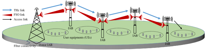
Figure 1: Multi-hop hybrid THz/FSO-based backhaul network with NLoS communication between the macro BS/donor IAB node and the final micro BS/child IAB node.

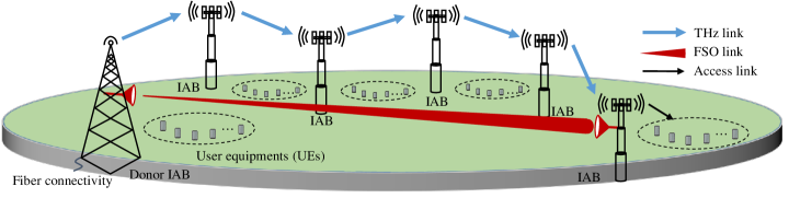
Figure 2: Multi-hop hybrid THz/FSO-based backhaul network with LoS communication between the macro BS/donor IAB node and the final micro BS/child IAB node.

From this perspective, this study focuses on the following:

• We first obtain closed-form and high signal-to-noise ratio (SNR) approximated probability density function (PDF) and cumulative distribution function (CDF) expressions of the FSO, the THz, and the mmWave access links’ SNR.

• Based on the derived PDF and CDF expressions, we derive the outage probability expressions for both system models of Figs. 1-2 as well as the mesh networks with both switching and combining methods between the parallel THz and FSO signals.

• Based on the high SNR approximated PDF and CDF expressions, we derive the asymptotic outage probability expressions for the considered system models with switching and combining methods between the parallel THz and FSO signals. Also, we find the diversity order for all considered setups.

• For both system models, the multi-hop analysis is extended to the mesh network by increasing the number of routes to improve the end-to-end (E2E) UE performance.

• Finally, we show the impact of atmospheric attenuation/path-loss, pointing/misalignment error, small-scale fading, atmospheric turbulence, number of RF antennas, number of UEs, number of hops, and the threshold data-rates on the performance of considered systems.

From the results, we observe that the parallel deployment of the THz/FSO links in the backhaul with proper system configuration improves the overall performance of the communication system. Also, the diversity order for combining and switching methods remains the same. However, depending on the network deployment, the combining method may provide a considerable performance gain compared to the switching method. Further, higher jitter standard deviation drastically reduces the performance of the THz, the FSO, and consequently the backhaul hybrid THz/FSO link. Then, the increase in number of hops increases the coverage area, however, reduces the E2E throughput. Also, mesh networks enable multiple routes and improve the coverage.

Table I consists of the notations considered throughout this work. The rest of the paper is organized as follows. Section II discusses the considered system and channel models. Then, the performance analysis of System-1 and System-2, shown in Figs. 1-2, are discussed in details in Section III and Section IV, respectively. Section V extends the performance of the considered systems to mesh networks. Then, the numerical and simulations results are shown and discussed in Section VI, and finally, the conclusions are drawn in Section VII.

TABLE I: Notations considered throughout the work.

Notation	Definition	Notation	Definition
$\text{j}\in\{\text{T},\text{F},\text{acc}\}$	The THz, FSO, or mmWave link’s selection parameter	$n$	Number of hops
$N_{\text{t}}$	Transmit antennas at the $n^{\text{th}}$ MiBS/child IAB	Q	Number of routes
$N_{\text{r}}$	Antennas at the $n^{\text{th}}$ MiBS/child IAB THz receiver	$\kappa$	FSO detector type
$P_{\text{j}_{n}}$	Transmit power at source j of $n^{\text{th}}$ hop	$L_{\text{j}_{n}}$	The j link length of $n^{\text{th}}$ hop
$G_{\text{t}}^{\text{j}_{n}}$	Transmit antenna gain at node j of $n^{\text{th}}$ hop	$G_{\text{r}}^{\text{j}_{n}}$	Receive antenna gain at node j of $n^{\text{th}}$ hop
$\alpha_{n}$,$\mu_{n}$	$n^{\text{th}}$ $\alpha-\mu$ distributed THz link’s fading coefficients	m	mmWave link’s fading parameter
$\alpha_{\text{F}_{n}}$,$\beta_{\text{F}_{n}}$	$n^{\text{th}}$ FSO link’s atmospheric turbulence parameters	$f_{\text{j}}$	Operating frequency of the j link
$\xi_{\text{j}}$,$A_{0,\text{j}}$	Pointing error parameters for the j link in $n^{\text{th}}$ hop	$\lambda_{\text{j}}$	Wavelength of the j link
$\omega_{\text{j}_{n}}$,$a_{\text{j}_{n}}$,$\varepsilon_{\text{j}_{n}}$	Beamwidth, receiver radius, and jitter standard deviation of j link	$\varrho_{\text{ox}}$	Oxygen absorption in mmWave link
$h_{\text{l}_{n}}$,$I_{\text{l}_{n}}$,$p_{\text{l}_{n}}$	Path-loss of the $n^{\text{th}}$ THz, FSO, and mmWave links	$\varrho_{\text{ra}}$	Rain attenuation in mmWave link
$\gamma_{\text{j}_{n}}$	Received SNR at node j in $n^{\text{th}}$ hop	c	Speed of light
$\gamma_{\text{th},n}$	SNR threshold at the $n^{\text{th}}$ FSO and THz receiver	$\gamma^{\text{UE}}_{\text{th}}$	SNR threshold at the mmWave UE

II System and Channel Models

We consider multi-hop hybrid THz/FSO networks to provide reliable high data-rates to the mmWave UEs (for the extension of the results to the cases with mesh networks, see Section V). We consider both non-IAB and out-band IAB-based communication setups. With a non-IAB setup, the relay nodes in between do not serve UEs and only forward backhaul data to the end relay node which is responsible for access communication to the UEs. With out-band IAB, on the other hand, while each relay node forwards backhaul data to following IAB nodes, it also provides access links to its surrounding UEs. With an IAB setup, the IAB donor is the node connecting to the core network via, for example, fiber links. Then, the nodes following the IAB donor in a multi-hop fashion are called IAB nodes (see Figs. 1-2). With a non-IAB setup, these nodes are referred to as macro BS (MaBS) and micro BS (MiBS), respectively.

For both non-IAB and IAB models, we consider two different network configurations:

• System 1: The MaBS/donor IAB node and the final MiBS/child IAB node communicate in NLoS manner. In this case, illustrated in Fig. 1, there are hybrid THz/FSO links in each backhaul link. Such a setup is of interest when there is no strong direct link between the MaBS/donor IAB and the final MiBS/child IAB node.

• System 2: The MaBS/donor IAB node and the final MiBS/child IAB node communicate in LoS manner. In this case, there is a direct FSO link between the MaBS and the final MiBS, as the FSO links can support long ranges. However, because with large hop distances, the THz links may not support the same order of rates as in the FSO links, we do not consider a direct THz link between the MaBS and final MiBS. Instead, in the THz, the data is forwarded to the final MiBS through multiple hops, as illustrated in Fig. 2.

Note that System-2 is of interest specially because, although we present the results for the general case with different number of hops, as we explain in the following, in practice multi-hop systems are of interest with a maximum of two hops. In such cases, it is probable to have a strong LoS connection between the first and last nodes, while due to the hop distance, the direct THz connection between these two nodes is not desirable. Moreover, the comparison between System 1 and 2 gives the chance to evaluate the benefits of multi-hop FSO communication.

Both heterodyne detection and intensity modulation/direct detection (IM/DD) methods are considered in the FSO links. Further, we consider DF relaying at each node to forward the successfully decoded signal from the previous node to the next node. For System-1 (resp. System-2) as shown in Fig. 1 (resp. Fig. 2), for each MiBS (resp. for the final MiBS), we consider different techniques for signal reception:

• Switching method: The receiver selects the best signal received through the THz or the FSO links and decodes it.

• Combination method: Based on the individual links SNR, the receiver may combine the signals received through the THz and FSO links.

II-A FSO Link Model

Considering the $n^{\text{th}}$ FSO link, the transmitted signal $s(t)$ received at the MiBS/child IAB node is expressed as

$$y_{{\text{F}_{n}}}\left(t\right)=\left({P_{\text{F}_{n}}}\eta I_{\text{l}_{n}}I_{n}\right)^{\frac{\kappa}{2}}s(t)+v_{\text{F}_{n}}\left(t\right),$$ (1)

where $P_{\text{F}_{n}}$ represents the transmit power at the $n^{\text{th}}$ FSO node and $\eta$ is the optical-to-electrical (O/E) conversion coefficient considered to be the same for all hops. Further, $I_{n}=I_{\text{p}_{n}}I_{\text{a}_{n}}$ represents the fading coefficient of the $n^{\text{th}}$ FSO link, where $I_{\text{p}_{n}}$ is the pointing error during the transmission and $I_{\text{a}_{n}}$ represents the fading due to the atmospheric turbulence. Also, $I_{\text{l}_{n}}$ is the atmospheric attenuation of the $n^{\text{th}}$ FSO link. Moreover, $\kappa=1$ and $\kappa=2$ represent the heterodyne detection and IM/DD, respectively, to write the generalized expressions for both the FSO detectors. Furthermore, $v_{\text{F}_{n}}(t)\sim\mathcal{N}(0,\sigma_{\text{o}}^{2})$ represents the additive white Gaussian noise (AWGN) associated with the $n^{\text{th}}$ FSO link with zero mean and $\sigma_{\text{o}}^{2}$ variance. For simplicity, we consider identical variance for all optical links. Hence, at the $n^{\text{th}}$ FSO receiver, the instantaneous received SNR will be $\gamma_{\text{F}_{n}}={\left(P_{\text{F}_{n}}\eta I_{\text{l}_{n}}I_{n}\right)^{\kappa}}/{\sigma^{2}_{\text{o}}}.$

II-A1 Atmospheric Attenuation

The atmospheric attenuation of the FSO link follows the Beer-Lambert Law [44] and is characterized as

$$I_{\text{l}_{n}}=\text{exp}\left(-\mathcal{C}_{\text{A}_{n}}L_{\text{F}_{n}}\right),$$ (2)

where, $L_{\text{F}_{n}}$ represents the $n^{\text{th}}$ FSO link length. Further, attenuation coefficient $\mathcal{C}_{\text{A}_{n}}$ is modeled as

$$\mathcal{C}_{\text{A}_{n}}=\frac{3.912}{\text{Vi}_{n}}\left(\frac{\lambda_{\text{F}_{n}}}{550}\right)^{\text{q}\left(\text{Vi}_{n}\right)}.$$ (3)

Here, for the $n^{\text{th}}$ FSO link, $\text{Vi}_{n}$ is the visibility with the visibility coefficient $\text{q}\left(\text{Vi}_{n}\right)$, where

$$\text{q}(\text{Vi}_{n})=\begin{cases}0.585\text{Vi}_{n}^{1/3},&\text{for }\text{Vi}_{n}<6\,\text{km}\\ 1.3,&\text{for }6<\text{Vi}_{n}<50\,\text{km}\\ 1.6,&\text{for }\text{Vi}_{n}>50\,\text{km}.\end{cases}$$ (4)

II-A2 Pointing/Misalignment Error

For the $n^{\text{th}}$-hop, we consider an $a_{\text{j}_{n}}$ aperture radius receiver situated $L_{\text{j}_{n}}$ distance apart from the transmitter. Hence, at the receiver, the received power from the transmitted $\omega_{\text{j}_{n}}$ beamwidth Gaussian beam is given as [45]

$$I_{\text{p,j}_{n}}\left(r_{\text{d},\text{j}_{n}};L_{\text{j}_{n}}\right)\approx A_{\text{0,j}_{n}}~{}\text{exp}\left(-{2r_{\text{d,j}_{n}}^{2}}/{\omega^{2}_{\text{eq},\text{j}_{n}}}\right),$$ (5)

where $r_{\text{d,j}_{n}}$ is the radial displacement between the detector and beam center for the $n^{\text{th}}$-hop. The $A_{\text{0,j}_{n}}=\left[\text{erf}(v_{0,\text{j}_{n}})\right]^{2}$ represents the fraction of the collected power at $r_{\text{d,j}_{n}}=0$ for the $n^{\text{th}}$-hop, where $v_{\text{0,j}_{n}}=\sqrt{{a_{\text{j}_{n}}^{2}\pi}/{(2\omega_{\text{j}_{n}}^{2})}}$ and $\text{erf}\left(x\right)=\frac{2}{\sqrt{\pi}}\int_{0}^{x}\exp\left(-z^{2}\right)\text{d}z$ is the error function. Further, the equivalent beamwidth is given as $\omega^{2}_{\text{eq},\text{j}_{n}}=\frac{\sqrt{A_{\text{0,j}_{n}}\pi}}{2v_{\text{0,j}_{n}}~{}\text{exp}(-v_{\text{0,j}_{n}}^{2})}\omega_{\text{j}_{n}}^{2}$. Note that for both FSO and THz links, the pointing/misalignment error modeling is considered to be similar and subscript $\text{j}\in[\text{F,T}]$ corresponds to the parameters for the FSO or THz links, respectively. However, the selection parameters may differ for both the THz and FSO links. Figure 3 depicts the pointing/misalignment error for the FSO/THz systems. Here, for the $n^{\text{th}}$-hop, $d_{\text{x,j}_{n}}$ is the beam displacement in the horizontal plane and $d_{\text{y,j}_{n}}$ is the beam displacement in the vertical plane. Consequently, the radial displacement vector is $r_{\text{d,j}_{n}}=\left[d_{\text{x,j}_{n}},d_{\text{y,j}_{n}}\right]^{\text{Tr}}$, where Tr is the transpose of a vector. If $d_{\text{x,j}_{n}}\approx\mathcal{N}\left(\varpi_{\text{x,j}_{n}},\varepsilon_{\text{x,j}_{n}}^{2}\right)$ and $d_{\text{y,j}_{n}}\approx\mathcal{N}\left(\varpi_{\text{y,j}_{n}},\varepsilon_{\text{y,j}_{n}}^{2}\right)$ are independently distributed Gaussian random variables (RVs), then $|r_{\text{d,j}_{n}}|=\sqrt{d_{\text{x,j}_{n}}^{2}+d_{\text{y,j}_{n}}^{2}}$ will be Beckmann distributed. Hence, different pointing error modeling are possible for different boresight and jitter values [46].

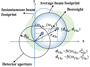
Figure 3: The misalignment/pointing error in the THz/FSO links.

Here, we consider that there is no boresight error, and jitters in horizontal and vertical directions are identical. This corresponds to $\varpi_{\text{x,j}_{n}}$ = $\varpi_{\text{y,j}_{n}}=0$ and $\varepsilon_{\text{x,j}_{n}}^{2}=\varepsilon_{\text{y,j}_{n}}^{2}=\varepsilon_{\text{j}_{n}}^{2}$ for the $n^{\text{th}}$-hop. Thus, the radial displacement is Rayleigh distributed and the PDF of pointing error is

$$f_{\text{I}_{\text{p,j}_{n}}}(x)=\frac{\xi_{\text{j}_{n}}^{2}}{A_{0,\text{j}_{n}}^{\xi_{\text{j}_{n}}^{2}}}x^{\xi_{\text{j}_{n}}^{2}-1},~{}~{}~{}~{}\text{for }0\leq x\leq A_{0,\text{j}_{n}}$$ (6)

where $\xi_{\text{j}_{n}}={\omega_{\text{eq},\text{j}_{n}}}/{(2\varepsilon_{\text{j}_{n}})}$ is a parameter related to the severity of pointing error.

II-A3 Exact PDF and CDF Expressions of FSO Link

We consider Gamma-Gamma distribution to model the atmospheric turbulence of the $n^{\text{th}}$ FSO link $I_{\text{a}_{n}}$, whose PDF is defined as

$$f_{I_{\text{a}_{n}}}(x) =\frac{2\left(\alpha_{\text{F}_{n}}\beta_{\text{F}_{n}}\right)^{\frac{\alpha_{\text{F}_{n}}+\beta_{\text{F}_{n}}}{2}}}{\Gamma(\alpha_{\text{F}_{n}})\Gamma(\beta_{\text{F}_{n}})}x^{\frac{\alpha_{\text{F}_{n}}+\beta_{\text{F}_{n}}}{2}-1}$$

$$\times\text{K}_{\alpha_{\text{F}_{n}}-\beta_{\text{F}_{n}}}\left(2\sqrt{\alpha_{\text{F}_{n}}\beta_{\text{F}_{n}}x}\right).$$ (7)

Here, $\Gamma(x)=\int_{0}^{\infty}z^{x-1}\exp\left(-z\right)\text{d}z$ represents complete Gamma function [47, (6.1.1)] and $\text{K}_{l}(x)=\frac{\Gamma\left(l+\frac{1}{2}\right)}{\sqrt{\pi}}\left(2x\right)^{l}\int_{0}^{\infty}\frac{\text{cos}(z)}{\left(x^{2}+z^{2}\right)^{l+\frac{1}{2}}}\text{d}z$ is the modified Bessel function of second kind with ${l}^{\text{th}}$ order [47, (9.6.25)]. The atmospheric turbulence’s fading coefficients for plane wave propagation are given as

$$\alpha_{\text{F}_{n}}=\left[\text{exp}\left(\frac{0.49\sigma_{\text{RV}_{n}}^{2}}{\left(1+1.11\sigma_{\text{RV}_{n}}^{12/5}\right)^{7/6}}\right)-1\right]^{-1},$$

$$\beta_{\text{F}_{n}}=\left[\text{exp}\left(\frac{0.51\sigma_{\text{RV}_{n}}^{2}}{\left(1+0.69\sigma_{\text{RV}_{n}}^{12/5}\right)^{5/6}}\right)-1\right]^{-1},$$ (8)

where the Rytov variance $\sigma_{\text{RV}_{n}}^{2}=1.23C_{{n}}^{2}k_{{0}_{n}}L_{\text{F}_{n}}^{11/6}$ represents the turbulence strength metric of the $n^{\text{th}}$ FSO link. Further, $k_{\text{0}_{n}}=2\pi/\lambda_{\text{F}_{n}}$ is the wave number and refractive index structure parameter $C_{{n}}^{2}$ corresponds to the strength of the atmospheric turbulence.

The fading coefficient $I_{n}=I_{\text{p}_{n}}I_{\text{a}_{n}}$ of the $n^{\text{th}}$ FSO link has the combined impact of the pointing error and the atmospheric turbulence. Hence, considering zero boresight error with identical jitters for the pointing error and Gamma-Gamma PDF for the atmospheric turbulence, for both detection techniques, the generalized PDF of the $n^{\text{th}}$ FSO link’s SNR is given by

$$f_{\gamma_{\text{F}_{n}}}(\gamma_{\text{F}_{n}}) =\frac{\xi^{2}_{\text{F}_{n}}}{\kappa\Gamma(\alpha_{\text{F}_{n}})\Gamma(\beta_{\text{F}_{n}})\gamma_{\text{F}_{n}}}$$

$$\times\text{G}^{3,0}_{1,3}\left[\frac{\alpha_{\text{F}_{n}}\beta_{\text{F}_{n}}}{A_{0{\text{F}_{n}}}}\left(\frac{\gamma_{\text{F}_{n}}}{\delta_{{\kappa}_{n}}}\right)^{\frac{1}{\kappa}}\Big{|}^{\xi^{2}_{\text{F}_{n}}+1}_{\xi^{2}_{\text{F}_{n}},\alpha_{\text{F}_{n}},\beta_{\text{F}_{n}}}\right],$$ (9)

where $\text{G}^{\hat{m},\hat{n}}_{\hat{p},\hat{q}}\left[z\big{|}^{a_{1},...,a_{\hat{n}},a_{\hat{n}+1},...,a_{\hat{p}}}_{b_{1},...,b_{\hat{m}},b_{\hat{m}+1},...,b_{\hat{q}}}\right]$ represents the Meijer-G function. Applying $F_{\gamma_{\text{F}_{n}}}(x)=\int_{0}^{x}f_{\gamma_{\text{F}_{n}}}(z)\text{d}z$ with [48, (07.34.21.0084.01)], the CDF of the $n^{\text{th}}$ FSO link’s SNR is given by

$$F_{\gamma_{\text{F}_{n}}}(\gamma_{\text{F}_{n}}) =\mathbb{D}^{n}_{1}\text{G}^{3\kappa,1}_{\kappa+1,3\kappa+1}\left[\frac{\mathbb{D}^{n}_{2}\gamma_{\text{F}_{n}}}{\left(A_{0{\text{F}}_{n}}\right)^{{\kappa}}\delta_{\kappa_{n}}}\Big{|}^{1,\Psi^{n}_{1}}_{\Psi^{n}_{2},0}\right],$$ (10)

where

$$\mathbb{D}^{n}_{1} =\frac{\kappa^{\left(\alpha_{\text{F}_{n}}+\beta_{\text{F}_{n}}-2\right)}\xi_{\text{F}_{n}}^{2}}{\left(2\pi\right)^{\kappa-1}\Gamma\left(\alpha_{\text{F}_{n}}\right)\Gamma\left(\beta_{\text{F}_{n}}\right)},\mathbb{D}^{n}_{2}=\frac{\left(\alpha_{\text{F}_{n}}\beta_{\text{F}_{n}}\right)^{\kappa}}{\kappa^{2\kappa}},$$

$$\Psi^{n}_{1} =\left[\frac{\xi_{\text{F}_{n}}^{2}+1}{\kappa},...,\frac{\xi_{\text{F}_{n}}^{2}+\kappa}{\kappa}\right],\Psi^{n}_{2}=\Big{[}\frac{\xi_{\text{F}_{n}}^{2}}{\kappa},...,\frac{\xi_{\text{F}_{n}}^{2}+\kappa-1}{\kappa},$$

$$\frac{\alpha_{\text{F}_{n}}}{\kappa},...,\frac{\alpha_{\text{F}_{n}}+\kappa-1}{\kappa},\frac{\beta_{\text{F}_{n}}}{\kappa},...,\frac{\beta_{\text{F}_{n}}+\kappa-1}{\kappa}\Big{]},$$ (11)

II-A4 High SNR PDF and CDF Expressions of the FSO Link

At high SNRs, the Meijer-G function can be approximated as [48, (07.34.06.0001.01)]. Hence, the PDF and CDF of the $n^{\text{th}}$ FSO link are approximated as

$$f^{A}_{\gamma_{\text{F}_{n}}}(\gamma_{\text{F}_{n}})\approx\frac{\xi^{2}_{\text{F}_{n}}}{\kappa\Gamma(\alpha_{\text{F}_{n}})\Gamma(\beta_{\text{F}_{n}})\gamma_{\text{F}_{n}}}$$

$$\times\sum_{p=1}^{3}\left(\frac{\alpha_{\text{F}_{n}}\beta_{\text{F}_{n}}}{A_{0{\text{F}_{n}}}}\left(\frac{\gamma_{\text{F}_{n}}}{\delta_{{\kappa}_{n}}}\right)^{\frac{1}{\kappa}}\right)^{\Psi^{n}_{4,p}}\frac{\overset{3}{\underset{\underset{q\neq p}{q=1}}{\prod}}\Gamma(\Psi^{n}_{4,q}-\Psi^{n}_{4,p})}{\overset{1}{\underset{q=1}{\prod}}\Gamma(\Psi^{n}_{3,q}-\Psi^{n}_{4,p})},$$ (12)

$$F^{\text{A}}_{\gamma_{\text{F}_{n}}}(\gamma_{\text{F}_{n}})\approx\mathbb{D}^{n}_{1}\sum_{p=1}^{3\kappa}\left(\frac{\mathbb{D}^{n}_{2}\gamma_{\text{F}_{n}}}{(A_{{0\text{F}}_{n}})^{\kappa}\delta_{\kappa_{n}}}\right)^{\Psi^{n}_{6,p}}$$

$$\times\frac{\overset{3\kappa}{\underset{\underset{q\neq p}{q=1}}{\prod}}\Gamma(\Psi^{n}_{6,q}-\Psi^{n}_{6,p})\overset{1}{\underset{q=1}{\prod}}\Gamma(1-\Psi^{n}_{5,q}+\Psi^{n}_{6,p})}{\overset{\kappa+1}{\underset{q=2}{\prod}}\Gamma(\Psi^{n}_{5,q}-\Psi^{n}_{6,p})\overset{3\kappa+1}{\underset{q=3\kappa+1}{\prod}}\Gamma(1-\Psi^{n}_{6,q}+\Psi^{n}_{6,p})},$$ (13)

where, $\Psi^{n}_{3}=[\xi_{\text{F}_{n}}^{2}+1]$, $\Psi^{n}_{4}=[\xi_{\text{F}_{n}}^{2},\alpha_{\text{F}_{n}},\beta_{\text{F}_{n}}]$, $\Psi^{n}_{5}=[1,\Psi^{n}_{1}]$, and $\Psi^{n}_{6}=[\Psi^{n}_{2},0]$ for the $n^{\text{th}}$ FSO link. Further, $\Psi^{n}_{3,p}$/$\Psi^{n}_{3,q}$, $\Psi^{n}_{4,p}$/$\Psi^{n}_{4,q}$, $\Psi^{n}_{5,p}$/$\Psi^{n}_{5,q}$, and $\Psi^{n}_{6,p}$/$\Psi^{n}_{6,q}$ represent the $p^{\text{th}}$/$q^{\text{th}}$ entry of $\Psi^{n}_{3}$, $\Psi^{n}_{4}$, $\Psi^{n}_{5}$, and $\Psi^{n}_{6}$, respectively. From (13), the high SNR CDF can be represented as $\approx(G_{\text{c}}\times\delta_{\kappa_{n}})^{-G_{\text{d}}}$ with $G_{\text{d}}$ and $G_{\text{c}}$ being the diversity and coding gains, respectively. Here, $G_{\text{d}}$ can be decided by $\Psi^{n}_{6}=[\Psi^{n}_{2},0]=\left[\frac{\xi_{\text{F}_{n}}^{2}}{\kappa},...,\frac{\xi_{\text{F}_{n}}^{2}+\kappa-1}{\kappa},\frac{\alpha_{\text{F}_{n}}}{\kappa},...,\frac{\alpha_{\text{F}_{n}}+\kappa-1}{\kappa},\frac{\beta_{\text{F}_{n}}}{\kappa},...,\frac{\beta_{\text{F}_{n}}+\kappa-1}{\kappa},0\right]$. Further, $F^{\text{A}}_{\gamma_{\text{F}_{n}}}(\gamma_{\text{F}_{n}})$ has $3\kappa$ summation terms, hence, the diversity order of the $n^{\text{th}}$ FSO link is $\min\left(\frac{\xi_{\text{F}_{n}}^{2}}{\kappa},\frac{\alpha_{\text{F}_{n}}}{\kappa},\frac{\beta_{\text{F}_{n}}}{\kappa}\right).$

II-B THz Link

To compensate for the large path-loss at the sub-THz bands, we deploy $N_{\text{r}}$ antennas at the THz receiver with maximum ratio combining (MRC). Considering the $n^{\text{th}}$ THz link, the transmitted signal $s(t)$ received at the MiBS/child IAB node is given by

$$y_{\text{T}_{n}}(t)=\sqrt{P_{\text{T}_{n}}}h_{\text{l}_{n}}\sum_{i=1}^{N_{\text{r}}}h^{i}_{{\text{T}}_{{n}}}~{}s(t)+v_{\text{T}_{n}}(t),$$ (14)

where $P_{\text{T}_{n}}$ is the transmitted power from the $n^{\text{th}}$ THz source node with $h_{\text{l}_{n}}$ being the path-loss. Further, for the $n^{\text{th}}$-hop, $h^{i}_{\text{T}_{n}}=h^{i}_{\text{f}_{n}}h^{i}_{\text{p}_{n}}$ is the fading coefficient of the THz link to the $i^{\text{th}}$ receiving antenna that has the combined impact of channel fading $h^{i}_{\text{f}_{n}}$ and antenna misalignment $h^{i}_{\text{p}_{n}}$. The THz transmitter and receiver are not very far and the receiving antennas are deployed close to each other. Hence, the same pointing error is considered at each receiving antenna. Therefore, the combined channel gain can be written as $||h_{\text{T}_{n}}||^{2}=h_{\text{p}_{n}}^{2}\sum_{i=1}^{N_{\text{r}}}|h^{i}_{\text{f}_{n}}|^{2}$. Further, $v_{\text{T}_{n}}(t)$ is the AWGN associated with the $n^{\text{th}}$ THz link having 0 mean and $\sigma_{\text{T}}^{2}$ variance. Note that, for simplicity, the identical AWGN variance $\sigma_{\text{T}}^{2}$ is considered in each hop. Performing MRC at the $n^{\text{th}}$ THz receiver, the instantaneous received SNR will be $\gamma_{\text{T}_{n}}=\sum_{i=1}^{N_{\text{r}}}\gamma^{i}_{\text{T}_{n}}={P_{\text{T}_{n}}h_{\text{l}_{n}}^{2}||h_{\text{T}_{n}}||^{2}}/{\sigma_{\text{T}}^{2}}.$

II-B1 Path-loss

The path-loss $h_{\text{l}_{n}}$ of the $n^{\text{th}}$ THz link is expressed as [41, 49]

$$h_{\text{l}_{n}}=\frac{c\sqrt{G^{\text{T}_{n}}_{\text{t}}G^{\text{T}_{n}}_{\text{r}}}}{4\pi f_{\text{T}_{n}}d_{\text{T}_{n}}}$$

$$\times\exp\left(-\frac{1}{2}d_{\text{T}_{n}}\left(\sum_{\hat{i}}\mathbb{F}_{\hat{i}}(f_{\text{T}_{n}},\nu)+\mathbb{G}(f_{\text{T}_{n}},\nu)\right)\right),$$ (15)

where $f_{\text{T}_{n}}$, $d_{\text{T}_{n}}$, $G^{\text{T}_{n}}_{\text{t}}$, and $G^{\text{T}_{n}}_{\text{r}}$ are the operational frequency, link length, transmit antenna gain, and receive antenna gain of the $n^{\text{th}}$ THz link, respectively. Here, $\mathbb{G}_{\hat{i}}(f_{\text{T}},\nu)$ is a fitting polynomial to match (II-B1) with the actual response. Further, at 119, 183, 325, 380, 439, and 448 GHz frequencies, the six major absorption lines are shown by the set of polynomials $\mathbb{F}_{\hat{i}}(f_{\text{T}_{n}},\nu)$. These parameters are described in [50, Section II].

II-B2 Exact PDF and CDF expressions of the THz Link

We consider the experimentally validated $\alpha-\mu$ fading to characterize each of the THz link’s gain [51]. Performing MRC at the THz receiver, the sum of $N_{\text{r}}$ RVs with $\alpha-\mu$ distributions is also approximated with a single $\alpha-\mu$ RV. Further, the same statistical modeling can be considered for the misalignment error associated with the THz link as shown in Fig. 3. Hence, we consider the Rayleigh distributed misalignment error for the THz link whose PDF is given in (6).

Considering the combined impact of $\alpha-\mu$ distributed channel fading with Rayleigh distributed misalignment error, the PDF of the SNR of the $n^{\text{th}}$ THz link is obtained as

$$f_{\gamma_{\text{T}_{n}}}(\gamma_{\text{T}_{n}}) =\frac{\mathbb{C}^{n}_{1}}{2(\hat{\gamma}_{\text{T}_{n}})^{\frac{\xi_{\text{T}_{n}}^{2}}{2}}}\gamma_{\text{T}_{n}}^{\frac{\xi_{\text{T}_{n}}^{2}}{2}-1}\Gamma\left(\mathbb{C}^{n}_{2},\mathbb{C}^{n}_{3}\left(\frac{\gamma_{\text{T}_{n}}}{\hat{\gamma}_{\text{T}_{n}}}\right)^{\frac{\alpha_{n}}{2}}\right),$$ (16)

where $\Gamma\left(a,x\right)=\int_{x}^{\infty}z^{a-1}\exp\left(-z\right)\text{d}z$ is the upper incomplete Gamma function. Here, $\mathbb{C}^{n}_{1}=\frac{\xi^{2}_{\text{T}_{n}}}{\left(A_{0,\text{T}_{n}}\right)^{\xi^{2}_{\text{T}_{n}}}}\frac{(N_{\text{r}}\mu_{n})^{\xi^{2}_{\text{T}_{n}}/\alpha_{n}}}{\Omega_{n}^{\xi^{2}_{\text{T}_{n}}}\Gamma(N_{\text{r}}\mu_{n})}$, $\mathbb{C}^{n}_{2}=\frac{\alpha_{n}N_{\text{r}}\mu_{n}-\xi^{2}_{\text{T}_{n}}}{\alpha_{n}}$, $\mathbb{C}^{n}_{3}=\frac{N_{\text{r}}\mu_{n}}{\left(A_{{0,\text{T}}_{n}}\right)^{\alpha_{n}}\Omega_{n}^{\alpha_{n}}}$, $\hat{\gamma}_{\text{T}_{n}}=N_{\text{r}}{\bar{\gamma}}_{\text{T}_{n}}$, and $\Omega_{n}$ is the $\alpha_{n}$-root mean value of the fading channel of the $n^{\text{th}}$-hop RVs with $\alpha-\mu$ distributions. Applying $F_{\gamma_{\text{F}_{n}}}(x)=\int_{0}^{x}f_{\gamma_{\text{F}_{n}}}(z)\text{d}z$, CDF of the $n^{\text{th}}$ THz link is derived as

$$F_{\gamma_{\text{T}_{n}}}(\gamma_{\text{T}_{n}}) =\frac{\mathbb{C}^{n}_{1}}{\xi_{\text{T}_{n}}^{2}}\Bigg{[}\left(\frac{\gamma_{\text{T}_{n}}}{{\hat{\gamma}}_{\text{T}_{n}}}\right)^{\frac{\xi_{\text{T}_{n}}^{2}}{2}}\Gamma\left(\mathbb{C}^{n}_{2},\mathbb{C}^{n}_{3}\left(\frac{\gamma_{\text{T}_{n}}}{{\hat{\gamma}}_{\text{T}_{n}}}\right)^{\frac{\alpha_{n}}{2}}\right)$$

$$+{\left(\mathbb{C}^{n}_{3}\right)}^{-\frac{\xi_{\text{T}_{n}}^{2}}{\alpha_{n}}}\Upsilon\left(N_{\text{r}}\mu_{n},\mathbb{C}^{n}_{3}\left(\frac{\gamma_{\text{T}_{n}}}{{\hat{\gamma}}_{\text{T}_{n}}}\right)^{\frac{\alpha_{n}}{2}}\right)\Bigg{]},$$ (17)

where $\Upsilon\left(a,x\right)=\int_{0}^{x}z^{a-1}\exp\left(-z\right)\text{d}z$ is the lower incomplete gamma function.

In Meijer-G form, the CDF of the $n^{\text{th}}$ THz link’s SNR can also be represented as

$$F_{\gamma_{\text{T}_{n}}}(\gamma_{\text{T}_{n}}) =\frac{\mathbb{C}^{n}_{1}}{\alpha_{n}({\hat{\gamma}}_{\text{T}_{n}})^{\frac{\xi_{\text{T}_{n}}^{2}}{2}}}\gamma_{\text{T}_{n}}^{\frac{\xi_{\text{T}_{n}}^{2}}{2}}$$

$$\times\text{G}^{2,1}_{2,3}\left[\mathbb{C}^{n}_{3}\left(\frac{\gamma_{\text{T}_{n}}}{{\hat{\gamma}}_{\text{T}_{n}}}\right)^{\frac{\alpha_{n}}{2}}\Big{|}^{1-\frac{\xi_{\text{T}_{n}}^{2}}{\alpha_{n}},1}_{0,\mathbb{C}^{n}_{2},-\frac{\xi_{\text{T}_{n}}^{2}}{\alpha_{n}}}\right].$$ (18)

II-B3 High SNR PDF and CDF expressions of the THz Link

Using $\Gamma(m,x)\underset{\overset{x\rightarrow 0}{}}{\approx}\left(\Gamma(m)-\frac{x^{m}}{m}\right)$ at high SNR, the $n^{\text{th}}$ THz link’s PDF (16) can be approximated as

$$f^{\text{A}}_{\gamma_{\text{T}_{n}}}(\gamma_{\text{T}_{n}}) \approx\frac{\mathbb{C}^{n}_{1}}{2({\hat{\gamma}}_{\text{T}_{n}})^{\frac{\xi_{\text{T}_{n}}^{2}}{2}}}\gamma_{\text{T}_{n}}^{\frac{\xi_{\text{T}_{n}}^{2}}{2}-1}$$

$$\times\left(\Gamma(\mathbb{C}^{n}_{2})-\frac{{\left(\mathbb{C}^{n}_{3}\right)}^{\mathbb{C}^{n}_{2}}}{\mathbb{C}^{n}_{2}}\left(\frac{\gamma_{\text{T}}}{{\hat{\gamma}}_{\text{T}_{n}}}\right)^{\frac{\mathbb{C}^{n}_{2}\alpha_{n}}{2}}\right).$$ (19)

Using $F^{\text{A}}_{\gamma_{\text{T}_{n}}}(\gamma_{\text{T}_{n}})=\int_{0}^{\gamma_{\text{T}_{n}}}f^{\text{A}}_{\gamma_{\text{T}_{n}}}(z)\text{d}z$, at high SNRs, the $n^{\text{th}}$ THz link’s CDF is approximated as

$$F^{\text{A}}_{\gamma_{\text{T}_{n}}}(\gamma_{\text{T}_{n}}) \approx\frac{\mathbb{C}^{n}_{1}\Gamma(\mathbb{C}^{n}_{2})}{\xi_{\text{T}_{n}}^{2}}\left(\frac{\gamma_{\text{T}_{n}}}{{\hat{\gamma}}_{\text{T}_{n}}}\right)^{\frac{\xi_{\text{T}_{n}}^{2}}{2}}$$

$$-\frac{\mathbb{C}^{n}_{1}{\left(\mathbb{C}^{n}_{3}\right)}^{\mathbb{C}^{n}_{2}}}{\mathbb{C}^{n}_{2}\left(\alpha_{n}N_{\text{r}}\mu_{n}\right)}\left(\frac{\gamma_{\text{T}_{n}}}{{\hat{\gamma}}_{\text{T}_{n}}}\right)^{\frac{\alpha_{n}N_{\text{r}}\mu_{n}}{2}}.$$ (20)

From (II-B3), the high SNR CDF can be represented as $\approx(G_{\text{c}}\times\hat{\gamma}_{\text{T}_{n}})^{-G_{\text{d}}}$. Hence, the diversity order of the $n^{\text{th}}$ THz link is $\min\left(\frac{\xi_{\text{T}_{n}}^{2}}{2},\frac{\alpha_{n}N_{\text{r}}\mu_{n}}{2}\right)$.

II-C mmWave Access Links

We deploy multiple RF antennas ($N_{\text{t}}$) at each MiBS/child IAB node for mmWave transmission to the UEs, which has single antenna due to the small size. Then, with $\hat{s}(t)$ being the successfully decoded signal at the $n^{\text{th}}$ MiBS/child IAB node, the $l^{\text{th}}$ UE receives the signal after maximal ratio transmission (MRT) as

$$y_{\text{I}_{n}\text{U}_{l}}\left(t\right)=\sqrt{P_{\text{acc}}p_{\text{l}}}\sum_{k=1}^{N_{\text{t}}}h_{{\text{k}_{n}\text{U}_{l}}}\hat{s}(t)+v_{\text{U}_{l}}(t),$$ (21)

where $p_{\text{l}}$ represents the gain of the path-loss in mmWave access link and $P_{\text{acc}}$ is the transmit power at the MiBS/child IAB node. Further, $h_{{\text{k}_{n}\text{U}_{l}}}$ is the fading coefficient of the $k^{\text{th}}$ antenna in $n^{\text{th}}$ hop to the $l^{\text{th}}$ UE and $v_{\text{U}_{l}}(t)$ is the zero mean and $\sigma_{\text{acc}}^{2}$ variance AWGN of the $l^{\text{th}}$ UE’s receiver. We consider Gamma distributed mmWave access link’s gain, i.e., $\mathcal{G}(m,\Omega_{\text{acc}})$, where $m$ is the fading severity and $\Omega_{\text{acc}}$ is the average power. We consider that all UEs are independent and identically distributed, hence, the same fading severity $m$ and average power is considered for each UE. At the $l^{\text{th}}$ UE, a single Gamma RV $\approx\mathcal{G}(mN_{\text{t}},\Omega_{\text{acc}})$ can approximate the sum of $N_{\text{t}}$ Gamma RVs. Hence, the received SNR at $l^{\text{th}}$ UE is $\gamma_{\text{acc}}={P_{\text{acc}}p_{\text{l}}||h_{\text{acc}}||^{2}}/{\sigma_{\text{acc}}^{2}}$ with $||h_{\text{acc}}||^{2}=\sum_{k=1}^{N_{\text{t}}}|h_{{\text{k}_{n}\text{U}_{l}}}|^{2}$ with the following PDF and CDF

$$f_{\gamma_{\text{I}_{n}\text{U}_{l}}}(\gamma_{\text{acc}}) =\frac{1}{\Gamma\left(mN_{\text{t}}\right)}\left(\frac{m}{\bar{\gamma}_{\text{acc}}}\right)^{mN_{\text{t}}}\gamma_{\text{acc}}^{mN_{\text{t}}-1}\exp{\left(-\frac{m}{\bar{\gamma}_{\text{acc}}}\gamma_{\text{acc}}\right)},$$ (22)

$$~{}~{}~{}F_{\gamma_{\text{I}_{n}\text{U}_{l}}}(\gamma_{\text{acc}}) =1-\frac{1}{\Gamma\left(mN_{\text{t}}\right)}\Gamma\left(mN_{\text{t}},\frac{m}{\bar{\gamma}_{\text{acc}}}\gamma_{\text{acc}}\right),$$ (23)

respectively, where $\bar{\gamma}_{\text{acc}}={\Omega_{\text{acc}}P_{\text{acc}}p_{\text{l}}}/{\sigma_{\text{acc}}^{2}}$ is the average received SNR.

II-C1 Path-loss

The gain of the path-loss $p_{\text{l}}$ for the mmWave access link is given as [52]

$$p_{\text{l}}[\text{dB}]=G^{\text{acc}}_{\text{t}}+G^{\text{acc}}_{\text{r}}-20\log_{10}\left(\frac{4\pi L_{\text{acc}}}{\lambda_{\text{acc}}}\right)-\left(\varrho_{\text{ox}}+\varrho_{\text{ra}}\right)L_{\text{acc}},$$ (24)

where $G^{\text{acc}}_{\text{t}}$, $G^{\text{acc}}_{\text{r}}$, $\lambda_{\text{acc}}$, and $L_{\text{acc}}$ are the transmit antenna gain, receiver antenna gain, wavelength, and the link distance of the mmWave access link, respectively. Also, $\varrho_{\text{ra}}$ and $\varrho_{\text{ox}}$ represent respectively the rain attenuation and the oxygen absorption.

III Performance Analysis of System-1

For System-1 (as shown in Fig. 1), we consider the MaBS/donor IAB and the final MiBS/child IAB are in NLoS. Hence, we deploy both the THz and the FSO links in parallel in each hop and the overall backhaul communication is completed through the serial multi-hop hybrid THz/FSO links with DF relaying. Further, we consider both switching and combining methods at the receiver, as explained in the following. We start the analysis for the multi-hop networks. Then, as explained in Section V, the results are extended to the cases with mesh networks.

III-A Combining Method

III-A1 Outage Probability

For the considered setup, the THz link is given higher priority and the FSO link is deployed to provide the backup to the THz link, if required. Hence, considering the $n^{\text{th}}$ hybrid THz/FSO backhaul link with combining method, the THz link works alone if its SNR is greater than or equal to an SNR threshold, i.e., $\gamma_{\text{T}_{n}}\geq\gamma_{\text{th},n}$, where $\gamma_{\text{th},n}$ is the threshold. However, with $\gamma_{\text{T}_{n}}<\gamma_{\text{th},n}$, receiver generates a feedback to activate the FSO link for simultaneous transmission along with the THz link if $\left(\gamma_{\text{T}_{n}}+\gamma_{\text{F}_{n}}\right)\geq\gamma_{\text{th},n}$. Therefore, for the $n^{\text{th}}$ backhaul hop, the instantaneous received SNR $\left(\gamma^{\text{CO}}_{\text{I}_{n}}\right)$ of the hybrid THz/FSO link is given as

$$\gamma^{\text{CO}}_{\text{I}_{n}}=\begin{cases}\gamma_{\text{T}_{n}},&\text{for }\gamma_{\text{T}_{n}}\geq\gamma_{\text{th},n}\\ \left(\gamma_{\text{T}_{n}}+\gamma_{\text{F}_{n}}\right),&\text{for }\gamma_{\text{T}_{n}}<\gamma_{\text{th},n}~{}\&~{}\left(\gamma_{\text{T}_{n}}+\gamma_{\text{F}_{n}}\right)\geq\gamma_{\text{th},n}\\ 0,&\text{for }\left(\gamma_{\text{T}_{n}}+\gamma_{\text{F}_{n}}\right)<\gamma_{\text{th},n}.\end{cases}$$ (25)

With combining, outage probability of the $n^{\text{th}}$ hybrid THz/FSO backhaul link is calculated as

$$\mathcal{P}^{\text{CO}}_{\gamma_{\text{I}_{n}}}(\gamma_{\text{th},n}) =F^{\text{CO}}_{\gamma_{\text{I}_{n}}}(\gamma_{\text{th},n})=\mathcal{P}\left[\left(\gamma_{\text{T}_{n}}+\gamma_{\text{F}_{n}}\right)<\gamma_{\text{th},n}\right].$$ (26)

Then, (26) can be derived as

$$\mathcal{P}^{\text{CO}}_{\gamma_{\text{I}_{n}}}(\gamma_{\text{th},n}) =\mathbb{I}_{1}(\gamma_{\text{th},n})-\mathbb{I}_{2}(\gamma_{\text{th},n})+\mathbb{I}_{3}(\gamma_{\text{th},n}).$$ (27)

Here,

$$\mathbb{I}_{1}(\gamma_{\text{th},n}) =\mathbb{D}^{n}_{1}\frac{\mathbb{C}^{n}_{1}\Gamma\left(\mathbb{C}^{n}_{2}\right)}{\xi_{\text{T}_{n}}^{2}{{\bar{\gamma}}_{\text{T}_{n}}}^{\frac{\xi^{2}_{\text{T}_{n}}}{2}}}\Gamma(\mathbb{C}^{n}_{4})\gamma_{\text{th},n}^{\mathbb{C}^{n}_{4}-1}$$

$$\times\text{G}^{3\kappa,1}_{\kappa+1,3\kappa+1}\left[\frac{\mathbb{D}^{n}_{2}\gamma_{\text{F}_{n}}}{\left(A_{0{\text{F}_{n}}}\right)^{{\kappa}}\delta_{\kappa_{n}}}\Big{|}^{1,\Psi^{n}_{1}}_{\Psi^{n}_{2},1-\mathbb{C}^{n}_{4}}\right],$$

$$\mathbb{I}_{2}(\gamma_{\text{th},n}) =\mathbb{D}^{n}_{1}\frac{\mathbb{C}^{n}_{1}}{\xi_{\text{T}_{n}}^{2}{{\bar{\gamma}}_{\text{T}_{n}}}^{\frac{\xi^{2}_{\text{T}_{n}}}{2}}}\sum_{z_{1}=0}^{\infty}\frac{(-1)^{z_{1}}}{z_{1}!\left(\mathbb{C}^{n}_{2}+z_{1}\right)}\left(\frac{\mathbb{C}^{n}_{3}}{{{\bar{\gamma}}_{\text{T}_{n}}}^{\frac{\alpha_{n}}{2}}}\right)^{\mathbb{C}^{n}_{2}+z_{1}}$$

$$\times\Gamma(\mathbb{C}^{n}_{5})\gamma_{\text{th},n}^{\mathbb{C}^{n}_{5}-1}\text{G}^{3\kappa,1}_{\kappa+1,3\kappa+1}\left[\frac{\mathbb{D}^{n}_{2}\gamma_{\text{F}_{n}}}{\left(A_{0{\text{F}_{n}}}\right)^{{\kappa}}\delta_{\kappa_{n}}}\Big{|}^{1,\Psi^{n}_{1}}_{\Psi^{n}_{2},1-\mathbb{C}^{n}_{5}}\right],$$

$$\mathbb{I}_{3}(\gamma_{\text{th},n}) =\mathbb{D}^{n}_{1}\frac{\mathbb{C}^{n}_{1}{\left(\mathbb{C}^{n}_{3}\right)}^{-\frac{\xi_{\text{T}_{n}}^{2}}{\alpha_{n}}}}{\xi_{\text{T}_{n}}^{2}}\sum_{z_{2}=0}^{\infty}\frac{(-1)^{z_{2}}}{z_{2}!\left(N_{\text{r}}\mu_{n}+z_{2}\right)}$$

$$\times\left(\frac{\mathbb{C}^{n}_{3}}{{{\bar{\gamma}}_{\text{T}_{n}}}^{\frac{\alpha_{n}}{2}}}\right)^{N_{\text{r}}\mu_{n}+z_{2}}\Gamma(\mathbb{C}^{n}_{6})\gamma_{\text{th},n}^{\mathbb{C}^{n}_{6}-1}$$

$$\times\text{G}^{3\kappa,1}_{\kappa+1,3\kappa+1}\left[\frac{\mathbb{D}^{n}_{2}\gamma_{\text{F}_{n}}}{\left(A_{0{\text{F}_{n}}}\right)^{{\kappa}}\delta_{\kappa_{n}}}\Big{|}^{1,\Psi^{n}_{1}}_{\Psi^{n}_{2},1-\mathbb{C}^{n}_{6}}\right],$$ (28)

where $\mathbb{C}^{n}_{4}=\frac{\xi^{2}_{\text{T}_{n}}}{2}+1$, $\mathbb{C}^{n}_{5}=\frac{\xi^{2}_{\text{T}_{n}}}{2}+\frac{\alpha_{n}}{2}\left(\mathbb{C}^{n}_{2}+z_{1}\right)+1$, and $\mathbb{C}^{n}_{6}=\frac{\alpha_{n}}{2}\left(N_{\text{r}}\mu_{n}+z_{1}\right)+1$.

Substituting the identities $\mathbb{I}_{1}(\gamma_{\text{th},n})$, $\mathbb{I}_{2}(\gamma_{\text{th},n})$, and $\mathbb{I}_{3}(\gamma_{\text{th},n})$ in (27), outage probability of the $n^{\text{th}}$ hybrid THz/FSO backhaul link for the combining method is obtained.

Proof: See Appendix A.

With DF relaying, outage probability of the $N$-hop hybrid THz/FSO-based backhaul system in a non-IAB setup is obtained as

$$\mathcal{P}^{\text{CO}}_{\text{BH,S-1}} =1-\prod_{\underset{}{n=1}}^{\overset{}{N}}\left(1-F^{\text{CO}}_{\gamma_{\text{I}_{n}}}\left(\gamma_{\text{th},n}\right)\right).$$ (29)

Also, the E2E outage probability of the considered network at $l^{\text{th}}$ UE is derived as

$$\mathcal{P}^{\text{CO}}_{\text{E2E,S-1}}\left(\gamma^{\text{UE}}_{\text{th}}\right) =1-\left(1-\mathcal{P}^{\text{CO}}_{\text{BH,S-1}}\right)\times\left(1-F_{\gamma_{\text{acc}}}\left(\gamma^{\text{UE}}_{\text{th}}\right)\right),$$

$$=\mathcal{P}^{\text{CO}}_{\text{BH,S-1}}+F_{\gamma_{\text{acc}}}\left(\gamma^{\text{UE}}_{\text{th}}\right)-\mathcal{P}^{\text{CO}}_{\text{BH,S-1}}\times F_{\gamma_{\text{acc}}}\left(\gamma^{\text{UE}}_{\text{th}}\right).$$ (30)

Note. The outage probability in (III-A1) is for a non-IAB setup. However, with an IAB setup, we need to average the performance over the outage probabilities in each hop to find the overall network outage probability, i.e., with an $N$-hop network, the total outage probability, assuming the same number of UEs per node, is given by

$$\mathcal{P}_{\text{out}}^{\text{total}}=\frac{1}{N}\sum_{n=1}^{N}\mathcal{P}_{\text{out}}^{n},$$ (31)

with $\mathcal{P}_{\text{out}}^{n}$ given by (34), except for the case where the donor IAB serves the UEs. In that case, a direct access link exists between the donor and UEs, with outage probability given in (23).

Note. In an alternative method, one can always use both links simultaneously. In that case, outage probability is given by $\mathcal{P}\left[\left(\gamma_{\text{T}_{n}}+\gamma_{\text{F}_{n}}\right)<\gamma_{\text{th},n}\right]$ which ends up the same as in (27).

III-A2 Diversity Order for the Combining Method

For combining method, the asymptotic outage probability of System-1 is derived as

$$\mathcal{P}^{\text{CO,A}}_{\gamma_{\text{I}_{n}}}(\gamma_{\text{th},n}) \approx\int_{0}^{\gamma_{\text{th},n}}f^{\text{A}}_{\gamma_{\text{F}}}(\gamma)\times F^{\text{A}}_{\gamma_{\text{T}}}(\gamma_{\text{th},n}-\gamma)\text{d}\gamma.$$ (32)

This can be simplified as

$$\mathcal{P}^{\text{CO,A}}_{\gamma_{\text{I}_{n}}}(\gamma_{\text{th},n})\approx\sum_{p=1}^{3}\Theta_{1}(p)$$

$$\times\left[\Theta_{2}\left(\frac{\gamma_{\text{th},n}}{\bar{\gamma}}\right)^{\frac{\xi_{\text{T}_{n}}^{2}}{2}+\frac{\Psi_{4,p}}{\kappa}}-\Theta_{3}\left(\frac{\gamma_{\text{th},n}}{\bar{\gamma}}\right)^{\frac{\alpha_{n}N_{\text{r}}\mu_{n}}{2}+\frac{\Psi_{4,p}}{\kappa}}\right],$$ (33)

where $\Theta_{1}(p)=\frac{\xi^{2}_{\text{F}_{n}}}{\kappa\Gamma(\alpha_{\text{F}_{n}})\Gamma(\beta_{\text{F}_{n}})}\frac{\overset{3}{\underset{\underset{q\neq p}{q=1}}{\prod}}\Gamma(\Psi_{4,q}-\Psi_{4,p})}{\overset{1}{\underset{q=1}{\prod}}\Gamma(\Psi_{3,q}-\Psi_{4,p})}\left(\frac{\alpha_{\text{F}_{n}}\beta_{\text{F}_{n}}}{A_{0{\text{F}_{n}}}\Delta_{1}^{\frac{1}{\kappa}}}\right)^{\Psi_{4,p}}$, $\Theta_{2}=\frac{\mathbb{C}^{n}_{1}\Gamma(\mathbb{C}^{n}_{2})}{\xi_{\text{T}_{n}}^{2}{\left(\Delta_{2}\right)}^{\frac{\xi_{\text{T}_{n}}^{2}}{2}}}\text{B}\left(\frac{\xi_{\text{T}_{n}}^{2}}{2}+1,\frac{\Psi_{4,p}}{\kappa}\right)$, and
$\Theta_{3}=\frac{\mathbb{C}^{n}_{1}{\left(\mathbb{C}^{n}_{3}\right)}^{\mathbb{C}^{n}_{2}}}{\mathbb{C}^{n}_{2}\left(\alpha_{n}N_{\text{r}}\mu_{n}\right){\left(\Delta_{2}\right)}^{\frac{\alpha_{n}N_{\text{r}}\mu_{n}}{2}}}\text{B}\left(\frac{\alpha_{n}N_{\text{r}}\mu_{n}}{2}+1,\frac{\Psi_{4,p}}{\kappa}\right).$

Proof: See Appendix B

From (III-A2), the diversity order of the $n^{\text{th}}$ backhaul link with combining is obtained as

$$G^{\text{CO},n}_{\text{d}}=\underset{\overset{\text{diversity order of the nth FSO link}}{}}{\underbrace{\min\left(\frac{\xi_{\text{F}_{n}}^{2}}{\kappa},\frac{\alpha_{\text{F}_{n}}}{\kappa},\frac{\beta_{\text{F}_{n}}}{\kappa}\right)}}+\underset{\overset{\text{diversity order of the nth THz link}}{}}{\underbrace{\min\left(\frac{\xi_{\text{T}_{n}}^{2}}{2},\frac{\alpha_{n}N_{\text{r}}\mu_{n}}{2}\right)}}.$$ (34)

Here, the first and the second terms represent the diversity order of the $n^{\text{th}}$ FSO and THz links, respectively. Further, the sum operation represents that both FSO and THz links work in parallel. Also, the diversity order of the $N$-hop hybrid THz/FSO-based backhaul system is given as

$$G^{\text{CO}}_{\text{d,S-1}}=$$

$${\underset{\forall_{n=1}^{N}}{\min}}\left[\underset{\overset{\text{diversity order of the nth hybrid THz/FSO link}}{}}{\underbrace{\min\left(\frac{\xi_{\text{F}_{n}}^{2}}{\kappa},\frac{\alpha_{\text{F}_{n}}}{\kappa},\frac{\beta_{\text{F}_{n}}}{\kappa}\right)+\min\left(\frac{\xi_{\text{T}_{n}}^{2}}{2},\frac{\alpha_{n}N_{\text{r}}\mu_{n}}{2}\right)}}\right].$$ (35)

Here, the final minimum operation outside the bracket denotes that the diversity order of a multi-hop network is limited by the worst hop. Note that the diversity order is the same for the IAB and non-IAB setup because, at high-SNR, the performance is determined by the worst-case scenario which is the outage probability at the end of the multi-hop chain.

III-B Switching Method

III-B1 Outage Probability

Considering the $n^{\text{th}}$ hybrid THz/FSO backhaul link with switching, the THz link is active, if $\gamma_{\text{T}_{n}}\geq\gamma_{\text{th},n}$. However, with $\gamma_{\text{T}_{n}}<\gamma_{\text{th},n}$, receiver generates a feedback to switch off the THz link and activate the FSO link if $\gamma_{\text{F}_{n}}\geq\gamma_{\text{th},n}$. Hence, for the $n^{\text{th}}$ hybrid THz/FSO backhaul link, the instantaneous received SNR at the MiBS/IAB $\left(\gamma^{\text{SW}}_{\text{I}_{n}}\right)$ is

$$\gamma^{\text{SW}}_{\text{I}_{n}}=\begin{cases}\gamma_{\text{T}_{n}},&\text{for }\gamma_{\text{T}_{n}}\geq\gamma_{\text{th},n}\\ \gamma_{\text{F}_{n}},&\text{for }\gamma_{\text{T}_{n}}<\gamma_{\text{th},n}~{}\&~{}\gamma_{\text{F}_{n}}\geq\gamma_{\text{th},n}\\ 0,&\text{for }\gamma_{\text{T}_{n}}<\gamma_{\text{th},n}~{}\&~{}\gamma_{\text{F}_{n}}<\gamma_{\text{th},n}.\end{cases}$$ (36)

The hybrid THz/FSO link is in outage when the instantaneous received SNRs of both the THz and the FSO links (i.e., $\gamma_{\text{T}_{n}}$ and $\gamma_{\text{F}_{n}}$) are below thresholds. Therefore, the outage probability of the $n^{\text{th}}$ hybrid THz/FSO backhaul link is calculated as

$$\mathcal{P}^{\text{SW}}_{\gamma_{\text{I}_{n}}}(\gamma_{\text{th},n}) =F^{\text{SW}}_{\gamma_{\text{I}_{n}}}(\gamma_{\text{th},n})=\mathcal{P}\left[\gamma_{\text{T}_{n}}<\gamma_{\text{th},n}~{}\&~{}\gamma_{\text{F}_{n}}<\gamma_{\text{th},n}\right].$$ (37)

The THz and FSO links are statistically independent, hence, outage probability is obtained as

$$\mathcal{P}^{\text{SW}}_{\gamma_{\text{I}_{n}}}\left(\gamma_{\text{th},n}\right) =F_{\gamma_{\text{T}_{n}}}\left(\gamma_{\text{th},n}\right)\times F_{\gamma_{\text{F}_{n}}}\left(\gamma_{\text{th},n}\right).$$ (38)

Substituting (10) and (II-B2) in (38), outage probability of the $n^{\text{th}}$ hop is derived as

$$\mathcal{P}^{\text{SW}}_{\gamma_{\text{I}_{n}}}\left(\gamma_{\text{th},n}\right) =\frac{\mathbb{C}^{n}_{1}\mathbb{D}^{n}_{1}}{\alpha_{\text{T}_{n}}({\bar{\gamma}}_{\text{T}_{n}})^{\frac{\xi_{\text{T}_{n}}^{2}}{2}}}\gamma_{\text{th},n}^{\frac{\xi_{\text{T}_{n}}^{2}}{2}}$$

$$\times\text{G}^{2,1}_{2,3}\left[\mathbb{C}^{n}_{3}\left(\frac{\gamma_{\text{th},n}}{{\bar{\gamma}}_{\text{T}_{n}}}\right)^{\frac{\alpha_{\text{T}_{n}}}{2}}\Big{|}^{1-\frac{\xi^{2}_{\text{T}_{n}}}{\alpha_{n}},1}_{0,\mathbb{C}^{n}_{2},-\frac{\xi^{2}_{\text{T}_{n}}}{\alpha_{n}}}\right]$$

$$\times\text{G}^{3\kappa,1}_{\kappa+1,3\kappa+1}\left[\frac{\mathbb{D}^{n}_{2}\gamma_{\text{th},n}}{\left(A_{{0\text{F}_{n}}}\right)^{\kappa}\delta_{\kappa_{n}}}\Big{|}^{1,\Psi^{n}_{1}}_{\Psi^{n}_{2},0}\right].$$ (39)

Also, outage probability of the $N$-hop hybrid THz/FSO-based backhaul system is obtained as

$$\mathcal{P}^{\text{SW}}_{\text{BH,S-1}} =1-\overset{N}{\underset{n=1}{\prod}}\left(1-F^{\text{SW}}_{\gamma_{\text{I}_{n}}}\left(\gamma_{\text{th},n}\right)\right).$$ (40)

Finally, the E2E outage probability of System-1 at $l^{\text{th}}$ UE is obtained as

$$\mathcal{P}^{\text{SW}}_{\text{E2E,S-1}}\left(\gamma^{\text{UE}}_{\text{th}}\right) =1-\left(1-\mathcal{P}^{\text{SW}}_{\text{BH,S-1}}\right)\times\left(1-F_{\gamma_{\text{acc}}}\left(\gamma^{\text{UE}}_{\text{th}}\right)\right).$$ (41)

Note. Equation (41) gives the outage probability for the non-IAB setup where the UEs are served only by the end access point. The same as in (31), the outage probability in the out-band IAB setup is given by averaging the outage probability over all IAB donor and child IAB nodes.

III-B2 Diversity Order for the Switching Method

For the $n^{\text{th}}$ hybrid THz/FSO backhaul link, the asymptotic outage probability can be derived as

$$\mathcal{P}^{\text{SW,A}}_{\gamma_{\text{I}_{n}}}(\gamma_{\text{th},n}) \approx F^{\text{A}}_{\gamma_{\text{F}}}(\gamma_{\text{th},n})\times F^{\text{A}}_{\gamma_{\text{T}}}(\gamma_{\text{th},n}).$$ (42)

Substituting $F^{\text{A}}_{\gamma_{\text{F}}}(\gamma_{\text{th},n})$ and $F^{\text{A}}_{\gamma_{\text{T}}}(\gamma_{\text{th},n})$ from (13) and (II-B3), respectively, in (42), we obtain

$$\mathcal{P}^{\text{SW,A}}_{\gamma_{\text{I}_{n}}}(\gamma_{\text{th},n})\approx\mathbb{D}^{n}_{1}\sum_{p=1}^{3\kappa}\left(\frac{\mathbb{D}^{n}_{2}\gamma_{\text{th},n}}{(A_{0,\text{F}})^{\kappa}\delta_{{\kappa}}}\right)^{\Psi^{n}_{6,p}}$$

$$\times\frac{\overset{3\kappa}{\underset{\underset{q\neq p}{q=1}}{\prod}}\Gamma(\Psi^{n}_{6,q}-\Psi^{n}_{6,p})\overset{1}{\underset{q=1}{\prod}}\Gamma(1-\Psi^{n}_{5,q}+\Psi^{n}_{6,p})}{\overset{\kappa+1}{\underset{q=2}{\prod}}\Gamma(\Psi^{n}_{5,q}-\Psi^{n}_{6,p})\overset{3\kappa+1}{\underset{q=5\kappa+1}{\prod}}\Gamma(1-\Psi^{n}_{6,q}+\Psi^{n}_{6,p})}$$

$$\times\left[\frac{\mathbb{C}^{n}_{1}\Gamma(\mathbb{C}^{n}_{2})}{\xi_{\text{T}_{n}}^{2}}\left(\frac{\gamma_{\text{th},n}}{{\bar{\gamma}}_{\text{T}_{n}}}\right)^{\frac{\xi_{\text{T}_{n}}^{2}}{2}}-\frac{\mathbb{C}^{n}_{1}{\left(\mathbb{C}^{n}_{3}\right)}^{\mathbb{C}^{n}_{2}}}{\mathbb{C}^{n}_{2}\left(\alpha_{n}N_{\text{r}}\mu_{n}\right)}\left(\frac{\gamma_{\text{th},n}}{{\bar{\gamma}}_{\text{T}_{n}}}\right)^{\frac{\alpha_{n}N_{\text{r}}\mu_{n}}{2}}\right].$$ (43)

At high SNRs, we have $\bar{\gamma}\rightarrow\infty$. Consequently, the average received SNR of the THz and the FSO links tend to infinity, i.e, $\bar{\gamma}_{\text{T}_{n}},\delta_{\kappa_{n}}\rightarrow\infty$. Hence, considering $\bar{\gamma}_{\text{T}_{n}}=\Delta_{1}\bar{\gamma}$ and $\delta_{\kappa_{n}}=\Delta_{2}\bar{\gamma}$, where $\Delta_{1}$ and $\Delta_{2}$ are constants, (III-B2) can be modified as

$$\mathcal{P}^{\text{SW,A}}_{\gamma_{\text{I}_{n}}}(\gamma_{\text{th},n})\approx\sum_{p=1}^{3\kappa}\Theta_{4}(p)\times\bigg{[}\Theta_{5}\left(\frac{\gamma_{\text{th},n}}{\bar{\gamma}}\right)^{\Psi^{n}_{6,p}+\frac{\xi_{\text{T}_{n}}^{2}}{2}}$$

$$-\Theta_{6}\left(\frac{\gamma_{\text{th},n}}{\bar{\gamma}}\right)^{\Psi^{n}_{6,p}+\frac{\alpha_{n}N_{\text{r}}\mu_{n}}{2}}\bigg{]},$$ (44)

where $\Theta_{4}(p)=\mathbb{D}^{n}_{1}\frac{\overset{3\kappa}{\underset{\underset{q\neq p}{q=1}}{\prod}}\Gamma(\Psi^{n}_{6,q}-\Psi^{n}_{6,p})\overset{1}{\underset{q=1}{\prod}}\Gamma(1-\Psi^{n}_{5,q}+\Psi^{n}_{6,p})}{\overset{\kappa+1}{\underset{q=2}{\prod}}\Gamma(\Psi^{n}_{5,q}-\Psi^{n}_{6,p})\overset{3\kappa+1}{\underset{q=5\kappa+1}{\prod}}\Gamma(1-\Psi^{n}_{6,q}+\Psi^{n}_{6,p})}\\ \left(\frac{\mathbb{D}^{n}_{2}}{(A_{0,\text{F}})^{\kappa}\Delta_{1}}\right)^{\Psi^{n}_{6,p}}$, $\Theta_{5}=\frac{\mathbb{C}^{n}_{1}\Gamma(\mathbb{C}^{n}_{2})}{\xi_{\text{T}_{n}}^{2}\Delta_{2}^{\frac{\xi_{\text{T}_{n}}^{2}}{2}}}$, and $\Theta_{6}=\frac{\mathbb{C}^{n}_{1}{\left(\mathbb{C}^{n}_{3}\right)}^{\mathbb{C}^{n}_{2}}}{\mathbb{C}^{n}_{2}\left(\alpha_{n}N_{\text{r}}\mu_{n}\right)\Delta_{2}^{\frac{\alpha_{n}N_{\text{r}}\mu_{n}}{2}}}$.

From (III-B2), the diversity order of the $n^{\text{th}}$ hybrid THz/FSO backhaul link is given as

$$G^{\text{SW},n}_{\text{d}}=\min\left(\frac{\xi_{\text{F}_{n}}^{2}}{\kappa},\frac{\alpha_{\text{F}_{n}}}{\kappa},\frac{\beta_{\text{F}_{n}}}{\kappa}\right)+\min\left(\frac{\xi_{\text{T}_{n}}^{2}}{2},\frac{\alpha_{n}N_{\text{r}}\mu_{n}}{2}\right)$$ (45)

From (34) and (45), it is clear that the diversity order of the $n^{\text{th}}$ hybrid THz/FSO backhaul link for both the combining and switching methods is the same. However, combining provides additional SNR gain over switching, which we will see in Section VI. Finally, the diversity order of the $N$-hop hybrid THz/FSO-based backhaul system is given as

$$G^{\text{SW}}_{\text{d,S-1}}=$$

$$\underset{\overset{\forall_{n=1}^{N}}{}}{\min}\left[\underset{\overset{\text{diversity order of the nth hybrid THz/FSO link}}{}}{\underbrace{\min\left(\frac{\xi_{\text{F}_{n}}^{2}}{\kappa},\frac{\alpha_{\text{F}_{n}}}{\kappa},\frac{\beta_{\text{F}_{n}}}{\kappa}\right)+\min\left(\frac{\xi_{\text{T}_{n}}^{2}}{2},\frac{\alpha_{n}N_{\text{r}}\mu_{n}}{2}\right)}}\right].$$ (46)

IV Performance Analysis of System-2

For System-2 (as shown in Fig. 2), we consider the MaBS/donor IAB and the final MiBS/child IAB are in LoS. Hence, the backhaul communication takes place through $N$ cascaded THz links and a single FSO link, with proper combining at the final MiBS/IAB node. We analyze the performance of the proposed System-2 by combining both signals coming from the $N$ cascaded THz links and the single FSO link, or by switching between $N$ cascaded THz links or to the single FSO link for signal reception. Both cases are analyzed in the following.

IV-A Combining Method

IV-A1 Outage Probability

Since the FSO link is working as a backup for the cascaded THz links, first we check the availability of THz links in the multi-hop hybrid THz/FSO-based network. If all THz links experience good channel quality, the equivalent cascaded THz link serves irrespective of the FSO link. If the final THz link is below threshold given that all intermediate THz links experience good channel quality, we consider simultaneous transmission through the cascaded THz links and the FSO link. Also, if any of the intermediate THz link fails, the FSO link becomes active if $\gamma_{\text{F}}\geq\gamma_{\text{th},N}$. Therefore, for the considered System-2 with combining method, the instantaneous received SNR at the final MiBS/child IAB is given as (47), at the top of the next page.

$$\gamma^{\text{CO}}_{\text{CI}}=\begin{cases}\gamma_{\text{T}_{\text{eq}}},&\text{for }\forall_{n=1}^{N}~{}\gamma_{\text{T}_{n}}\geq\gamma_{\text{th},n}\\ \gamma_{\text{T}_{n}}+\gamma_{\text{F}},&\text{for }\forall_{n=1}^{N}\left({\gamma_{\text{T}_{n}}}<\gamma_{\text{th},n}~{}\&~{}\left(\gamma_{\text{T}_{n}}+\gamma_{\text{F}}\right)\geq\gamma_{\text{th},N}~{}\&~{}\gamma_{\text{T}_{n-1}}\geq\gamma_{\text{th},(n-1)}\right)\\ \gamma_{\text{F}},&\text{for }\forall_{n=1}^{N-1}\big{(}\gamma_{\text{T}_{n}}<\gamma_{\text{th},n}~{}\&~{}\gamma_{\text{F}}\geq\gamma_{\text{th},N}~{}\&~{}\gamma_{\text{T}_{n-1}}\geq\gamma_{\text{th},(n-1)}\big{)}\\ 0,&\text{for }\forall_{n=1}^{N-1}\big{(}\gamma_{\text{T}_{n}}<\gamma_{\text{th},n}~{}\&~{}\gamma_{\text{F}}<\gamma_{\text{th},N}~{}\&~{}\gamma_{\text{T}_{n-1}}\geq\gamma_{\text{th},(n-1)}\big{)}\\ &~{}{\text{or }}\forall_{n=1}^{N}\left(\left(\gamma_{\text{T}_{n}}+\gamma_{\text{F}}\right)<\gamma_{\text{th},N}~{}\&~{}\gamma_{\text{T}_{n-1}}\geq\gamma_{\text{th},(n-1)}\right),\end{cases}$$ (47)

Hence, the outage probability of the multi-hop THz/FSO backhaul network is found as

$$\mathcal{P}^{\text{CO}}_{\gamma_{\text{CI}}}=$$

$$\mathcal{P}\bigg{[}\forall_{n=1}^{N-1}\big{(}\gamma_{\text{T}_{n}}<\gamma_{\text{th},n}~{}\&~{}\gamma_{\text{F}}<\gamma_{\text{th},N}~{}\&~{}\gamma_{\text{T}_{n-1}}\geq\gamma_{\text{th},(n-1)}\big{)}$$

$$~{}{\text{or }}\forall_{n=1}^{N}\left(\left(\gamma_{\text{T}_{n}}+\gamma_{\text{F}}\right)<\gamma_{\text{th},N}~{}\&~{}\gamma_{\text{T}_{n-1}}\geq\gamma_{\text{th},(n-1)}\right)\bigg{]}.$$ (48)

This can be solved as

$$\mathcal{P}^{\text{CO}}_{\gamma_{\text{CI}}} =F_{\gamma_{\text{F}}}\left(\gamma_{\text{th},N}\right)\times\bigg{[}\sum_{n=1}^{N-1}F_{\gamma_{\text{T}_{n}}}\left(\gamma_{\text{th},n}\right)$$

$$\times\prod_{n_{1}=1}^{n-1}\left(1-F_{\gamma_{\text{T}_{(n-n_{1})}}}\left(\gamma_{\text{th},(n-n_{1})}\right)\right)\bigg{]}$$

$$+\prod_{n=1}^{N-1}\left(1-F_{\gamma_{\text{T}_{n}}}\left(\gamma_{\text{th},n}\right)\right)\times F^{\text{CO}}_{\gamma_{\text{I}_{N}}}.$$ (49)

Here, $F^{\text{CO}}_{\gamma_{\text{I}_{N}}}$ is the CDF by performing the combining between the $N^{\text{th}}$ THz link and the single FSO link at the final node which is calculated the same as in (26). Further, $F_{\gamma_{\text{T}_{n}}}\left(\gamma_{\text{th},n}\right)$ is the CDF of the $n^{\text{th}}$ THz link (II-B2) and $F_{\gamma_{\text{F}}}\left(\gamma_{\text{th},N}\right)$ is the CDF of the FSO link (10). Substituting (10), (II-B2), and (26) in (IV-A1), outage probability of backhaul links in System-2 is obtained.

Finally, the E2E outage probability of the considered network at $l^{\text{th}}$ UE is derived as

$$\mathcal{P}^{\text{CO}}_{\text{E2E,S-2}}\left(\gamma^{\text{UE}}_{\text{th}}\right) =1-\left(1-\mathcal{P}^{\text{CO}}_{\gamma_{\text{CI}}}\right)\times\left(1-F_{\gamma_{\text{acc}}}\left(\gamma^{\text{UE}}_{\text{th}}\right)\right).$$ (50)

Note that (50) gives the E2E outage probability for the cases with non-IAB based communication setup. Following (31), one can extend the results to the cases with IAB setup.

Finally, in an alternative method, one can always use both links simultaneously. In that case, the outage probability is given by $\mathcal{P}\Big{[}\forall_{n=1}^{N-1}\big{(}\gamma_{\text{T}_{n}}<\gamma_{\text{th},n}~{}\&~{}\gamma_{\text{F}}<\gamma_{\text{th},N}~{}\&~{}\gamma_{\text{T}_{n-1}}\geq\gamma_{\text{th},(n-1)}\big{)}~{}{\text{or }}\forall_{n=1}^{N}\left(\left(\gamma_{\text{T}_{n}}+\gamma_{\text{F}}\right)<\gamma_{\text{th},N}~{}\&~{}\gamma_{\text{T}_{n-1}}\geq\gamma_{\text{th},(n-1)}\right)\Big{]}$ which ends up in the same result as in (IV-A1).

IV-A2 Diversity Order for the Combining Method

The diversity order of the $N$ cascaded THz links is $\underset{\forall_{n=1}^{N}}{\min}\left(\frac{\xi_{\text{T}_{n}}^{2}}{2},\frac{\alpha_{n}N_{\text{r}}\mu_{n}}{2}\right)$. Further, the diversity order of the single FSO link is $\min\left(\frac{\xi_{\text{F}}^{2}}{\kappa},\frac{\alpha_{\text{F}}}{\kappa},\frac{\beta_{\text{F}}}{\kappa}\right)$. Thus, the overall diversity order of System-2 for the combining method is obtained as

$$G^{\text{ST}}_{\text{d,S-2}}=\underset{\overset{\text{diversity order of the single E2E FSO link}}{}}{\underbrace{\min\left(\frac{\xi_{\text{F}}^{2}}{\kappa},\frac{\alpha_{\text{F}}}{\kappa},\frac{\beta_{\text{F}}}{\kappa}\right)}}+\underset{\overset{\text{diversity order of the N cascaded THz links}}{}}{\underbrace{\underset{\forall_{n=1}^{N}}{\min}\left(\frac{\xi_{\text{T}_{n}}^{2}}{2},\frac{\alpha_{n}N_{\text{r}}\mu_{n}}{2}\right)}}.$$ (51)

IV-B Switching Method

IV-B1 Outage Probability

$$\gamma^{\text{SW}}_{\text{CI}}=\begin{cases}\gamma_{\text{T}_{\text{eq}}},&\text{for }{\forall_{n=1}^{N}~{}\gamma_{\text{T}_{n}}}\geq\gamma_{\text{th},n}\\ \gamma_{\text{F}},&\text{for }\forall_{n=1}^{N}\big{(}\gamma_{\text{T}_{n}}<\gamma_{\text{th},n}~{}\&~{}\gamma_{\text{F}}\geq\gamma_{\text{th}}~{}\&~{}\gamma_{\text{T}_{n-1}}\geq\gamma_{\text{th},(n-1)}\big{)}\\ 0,&\text{for }\forall_{n=1}^{N}\big{(}\gamma_{\text{T}_{n}}<\gamma_{\text{th},n}~{}\&~{}\gamma_{\text{F}}<\gamma_{\text{th}}~{}\&~{}\gamma_{\text{T}_{n-1}}\geq\gamma_{\text{th},(n-1)}\big{)}.\end{cases}$$ (52)

TABLE II: Considered parameters for the simulations.

THz link		FSO link		mmWave access link
Parameters	Value	Parameters	Value	Parameters	Value
$f_{\text{T}_{n}}$	119 GHz	$\lambda_{\text{F}_{n}}$	1550 nm	$f_{\text{acc}}$	28 GHz
$G_{\text{t}}^{\text{T}_{n}}$	55 dBi	Strong: $C_{n}^{2}$	1$\times 10^{-12}$m-2/3	$G_{\text{t}}^{\text{acc}}$	44 dBi
$G_{\text{r}}^{\text{T}_{n}}$	55 dBi	Moderate: $C_{n}^{2}$	5$\times 10^{-13}$m-2/3	$G_{\text{r}}^{\text{acc}}$	44 dBi
$p$	101325 Pa	Strong: $\alpha_{\text{F}_{n}}$,$\beta_{\text{F}_{n}}$	4.343, 2.492	$\varrho_{\text{ra}}$	0 dB/km
$T$	298 K	Moderate: $\alpha_{\text{F}_{n}}$,$\beta_{\text{F}_{n}}$	5.838, 4.249	$\varrho_{\text{ox}}$	15.1 dB/km
$\chi$	50$\%$	$\eta$	1
${a_{\text{T}_{n}}}$	${\lambda_{\text{T}_{n}}/{\left(2\pi\right)}\sqrt{G^{\text{T}_{n}}_{\text{t}}}}$	${a_{\text{F}_{n}}}$	20 cm
${\omega_{\text{T}_{n}}}$	50 cm	${\omega_{\text{F}_{n}}}$	40 cm
$\varepsilon_{\text{T}_{n}}$	6 cm	$\varepsilon_{\text{F}_{n}}$	5 cm

Since the FSO link is working as a backup for the THz link, first we check the availability of the THz link in the multi-hop hybrid THz/FSO-based backhaul network. If all THz nodes can decode the data correctly, the equivalent multi-hop THz link will serve irrespective of the FSO link. However, if any of the THz links fails, the FSO link becomes active if $\gamma_{\text{F}}\geq\gamma_{\text{th}}$. Therefore, for the considered System-2 with switching, the instantaneous received SNR at the final MiBS/child IAB is given as (52), at the top of this page. From this, the outage probability is calculated as

$$\mathcal{P}^{\text{SW}}_{\gamma_{\text{CI}}}\left(\gamma_{\text{th}}\right)=$$

$$\mathcal{P}\left[\forall_{n=1}^{N}\big{(}\gamma_{\text{T}_{n}}<\gamma_{\text{th},n}~{}\&~{}\gamma_{\text{F}}<\gamma_{\text{th}}~{}\&~{}\gamma_{\text{T}_{n-1}}\geq\gamma_{\text{th},(n-1)}\big{)}\right].$$

This can be solved as

$$\mathcal{P}^{\text{SW}}_{\gamma_{\text{CI}}}\left(\gamma_{\text{th}}\right) =F_{\gamma_{\text{F}}}\left(\gamma_{\text{th}}\right)\times\bigg{[}\sum_{n=1}^{N}F_{\gamma_{\text{T}_{n}}}\left(\gamma_{\text{th},n}\right)$$

$$\times\prod_{n_{1}=1}^{n-1}\left(1-F_{\gamma_{\text{T}_{(n-n_{1})}}}\left(\gamma_{\text{th},(n-n_{1})}\right)\right)\bigg{]}.$$ (54)

With non-IAB setup, the E2E outage probability of the considered network is derived as

$$\mathcal{P}^{\text{SW}}_{\text{E2E,S-2}}\left(\gamma^{\text{UE}}_{\text{th}}\right) =1-\left(1-\mathcal{P}^{\text{SW}}_{\gamma_{\text{CI}}}\right)\times\left(1-F_{\gamma_{\text{acc}}}\left(\gamma^{\text{UE}}_{\text{th}}\right)\right).$$ (55)

Finally, the same as in (31), the outage probability in the out-band IAB setup is given by averaging the outage probability over all IAB donor and child IAB nodes.

IV-B2 Diversity Order for the Switching Method

With DF relaying, the diversity order of the considered System-2 with switching is given as

$$G^{\text{SW}}_{\text{d,S-2}}=\underset{\overset{\text{diversity order of the single E2E FSO link}}{}}{\underbrace{\min\left(\frac{\xi_{\text{F}}^{2}}{\kappa},\frac{\alpha_{\text{F}}}{\kappa},\frac{\beta_{\text{F}}}{\kappa}\right)}}+\underset{\overset{\text{diversity order of the N cascaded THz links}}{}}{\underbrace{\underset{\forall_{n=1}^{N}}{\min}\left(\frac{\xi_{\text{T}_{n}}^{2}}{2},\frac{\alpha_{n}N_{\text{r}}\mu_{n}}{2}\right)}}.$$ (56)

Note that the diversity order of System-2 for both combining and switching methods is the same, which is already proved in Section III for System-1.

V Mesh Network

We consider a mesh network with $Q$ independent and non-overlapping multi-hop routes from the MaBS to the UE. The $q^{\text{th}}$ route ($q=1,2,...,Q$) consists of the multi-hop hybrid THz/FSO links according to System-1 and System-2. Thus, for the mesh network, outage probability is

$$\mathcal{P}^{\text{mesh}}_{\text{out}}=\prod_{q=1}^{Q}\mathcal{P}_{\text{out},q},$$ (57)

where $\mathcal{P}_{\text{out},q}$ is the outage probability of the $q^{\text{th}}$ E2E path from the MaBS to the destination UE. For System-1, this is derived in (III-A1) and (41) for the combining and the switching methods, respectively. For System-2, this is derived in (50) and (55) for the combining and the switching methods, respectively. Note that in (57) we have used the fact that in a mesh network an outage occurs if the data is correctly transferred to the destination through none of the routes and there is no overlap between the routes.

VI Simulation Results

We present our results with respect to the transmit power which is defined as $10\log_{10}\left({P_{\text{j}}}\right)$ in the log-domain. Here, $P_{\text{j}}$ with $\text{j}\in\{\text{T,F,acc}\}$ is the transmit power at the $j$ node. For simplicity, we consider $P_{\text{F}}=P_{\text{T}}=P_{\text{acc}}$ in each hop for the analysis. Further, $\sigma^{2}_{\text{o}}=\sigma^{2}_{\text{T}}=\sigma^{2}_{\text{acc}}=1$ is assumed in each hop. Rest of the simulation parameters are given in Table II. We present the results for the general cases with multi-hop and mesh networks. However, as demonstrated in [2, 3], with multi-hop and IAB networks, the system performance is significantly affected by increasing the number of hops, as the traffic congestion and E2E latency increases. For this reason, except for Fig. 4, where multi-hop results are shown for both the systems, only dual backhaul hops are considered for rest of the results. In Figs. 7-10, we present the results for the cases with IAB setup where each intermediate IAB node in the multi-hop setup serves a number of surrounding UEs. In Figs. 4-6, on the other hand, we present the results for the non-IAB setup where the UEs are served only by the end MiBS. Note that if the SNR threshold is fixed in all hops, we are in non-IAB case (even if the figure only presents the backhaul performance).

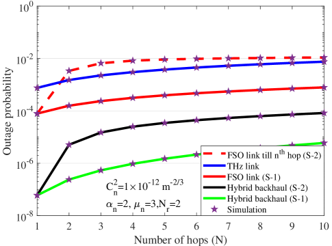
Figure 4: Impact of number of hops on the outage probability of the backhaul hybrid THz/FSO systems with switching. Here, we consider 200 m links in each hop, 25 dB transmit power, $\gamma_{\text{th}}=1$ in each hop, and present the results for both System 1 and 2. Also, $C_{n}^{2}=1\times 10^{-12}\text{m}^{-2/3}$ and $\alpha_{n}=2,\mu_{n}=3,N_{r}=2$.

In Fig. 4, we compare the outage probability of the multi-hop backhaul hybrid THz/FSO systems for different turbulence/fading conditions. We study both System-1 (S-1 in Figs.) and System-2 (S-2 in Figs.), as defined in Figs. 1-2, respectively. From Fig. 4, we observe that the FSO link’s performance decreases significantly for System-2 (shown with dotted red) as compared to System-1 (shown with solid red), where $N$ FSO links are deployed in DF mode. However, for both systems, $N$ THz links are deployed in series for the E2E backhaul communication, hence, the THz link’s performance remains the same (shown in blue for both systems). Consequently, the E2E performance of System-2 decreases significantly as compared to System-1. As shown in Fig. 4, for both systems, increasing the number of hops from 1 to 2 results in significant outage probability increment. However, for more than 2 hops, the outage probability is only slightly affected by increasing the number of hops. On the other hand, as discussed before and shown in [2, 3], the E2E delay/throughout are significantly deteriorated by increasing the number of hops.

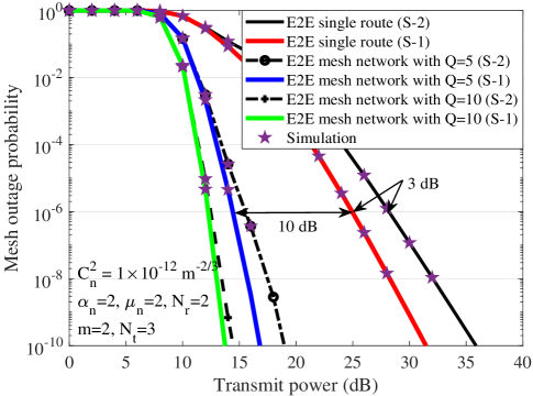
Figure 5: E2E outage probability of mesh network for both the systems with different routes by fixing 3 hops per route (2 backhaul and one access link) and by considering switching method. Here, $L_{\text{F}}=200$ m, $L_{\text{T}}=200$ m, and $L_{\text{acc}}=100$ m in each hop.

In Fig. 5, we show the E2E outage probability of mesh networks for both system models. Here, in each route, we fix the number of hops to three with two hybrid THz/FSO-based backhaul hops and one mmWave access hop. We consider strong turbulence/fading case by setting $C_{n}^{2}=1\times 10^{-12}$ m^-2/3 which gives $\alpha_{\text{F}}=4.34$, $\beta_{\text{F}}=2.49$ for the FSO links. Further, we consider $\alpha=2,\mu=2,N_{\text{r}}=2$ and $m=2,N_{\text{t}}=3$ for the THz and mmWave access links, respectively.

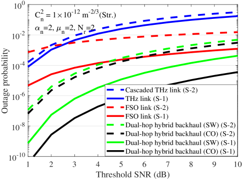
Figure 6: Comparison of outage probability of both the multi-hop THz/FSO-based systems against SNR threshold.

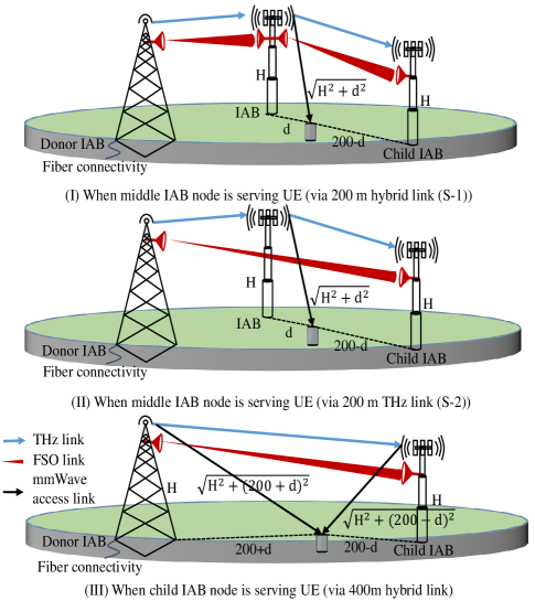
(a) Different cases with and without middle IAB node.

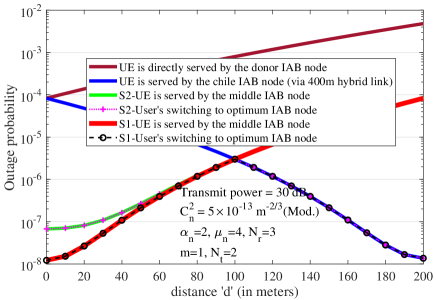
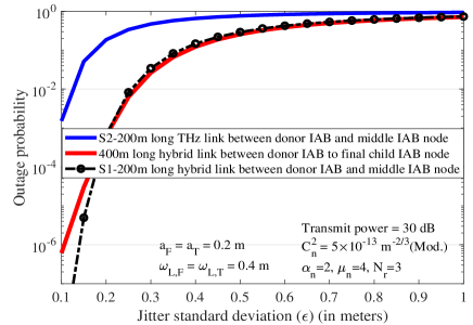
(b) Outage probability versus UE distance with respect to the middle IAB and child IAB nodes.

(c) Outage probability versus jitter standard deviation.

Figure 7: Comparison of both the hybrid THz/FSO-based dual-hop IAB networks with switching.

As compared to the single route multi-hop network (as shown in Fig. 4), whose outage performance degrades with number of hops, a mesh network improves the overall outage performance by enabling more routes. From Fig. 5, we observe that for the considered set of parameters and an outage probability $10^{-6}$, System-1 provides 3 dB gain over System-2 for a single route multi-hop network. Also, by increasing the E2E routes (Q=5) in the mesh network and outage probability $10^{-6}$, we obtain approximately 10 dB gain over the single route multi-hop network for both systems. Adding more routes will further improve the E2E performance, however, with a decreased rate than before. The results are shown for the switching case. With combining, we will achieve improved performance over switching, however, the qualitative insights remain the same.

In Fig. 6, we show the impact of SNR threshold on the outage performance of the dual-hop backhaul systems for both System-1 (solid lines) and System-2 (dotted lines) with both switching and combining methods. Here, we consider the same SNR threshold at each receiving MiBS node, hence, it is a non-IAB system. The FSO link of System-1 outperforms the FSO link of System-2, since, for the dual-backhaul hops, the FSO link in System-2 is approximately twice longer than the FSO link in System-1. Further, the cascaded THz link of System-2 (dual-hop) has slightly lower performance than the single THz link of System-1. Consequently, the dual-hop backhaul hybrid THz/FSO-based link of System-1 has better performance than System-2 for both the switching and combining methods. Further, we observe a significant performance improvement in System-1 with combining over the switching method at the receiving MiBS as compared to System-2. This is due to the fact, that in System-2, the switching/combining is performed at the end of the second hop, and the single THz link of the first hop dominates in the backhaul dual-hop communication. Hence, in this case, we observe only slight improvement in combining over switching in System-2.

(a) Different cases when UE lies in between the donor and middle IAB node.

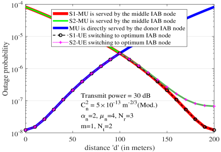
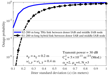
(b) Outage probability versus MU distance with respect to the middle IAB and child IAB nodes.

(c) Outage probability versus jitter standard deviation.

Figure 8: Comparison of both dual-hop IAB networks with switching.

In Figs. 4-6, we have shown the results of non-IAB multi-hop and mesh networks, where identical SNR threshold is considered on each of the receiving MiABs. On the other hand, Figs. 7-10 illustrate the results for IAB networks. With IAB, each IAB node carries the information of all UEs to be served by the IAB node itself and its following child IAB nodes. Different SNR thresholds consideration at each IAB node is motivated with the fact that the SNR threshold is directly related to the number of UEs associated with each IAB node. Let us assume a desired rate $\mathcal{R}$ bps/Hz at each UE, and $L$ such UEs are being served by the $n^{\text{th}}$ IAB node or its following child IAB nodes in the multi-hop chain. Then, the SNR threshold at the $n^{\text{th}}$ IAB node will be $\gamma_{\text{th},n}=2^{L\times\mathcal{R}}-1$. Thus, the SNR threshold of each IAB node is scaled by the total number of UEs which are served by the IAB node and its following child nodes.

Considering 10 UEs associated to each IAB node with $\mathcal{R}=0.1$ bps/Hz, we set the threshold at each IAB node. In Fig. 7(a), we show the movement of the UE in between the middle and last IAB nodes, and show the need of the middle IAB node. We consider that the height of the donor and the child IAB node is $H=30$ m, and the $l^{\text{th}}$ UE is at distance $d$ apart from the middle IAB node and moving towards the final IAB node. We consider the cases when the middle IAB node is serving the UE via 200 m hybrid THz/FSO link (System-1 (first case of Fig. 7(a))), the middle IAB node is serving the UE via 200 m THz link (System-2 (second case of Fig. 7(a))), and the final IAB node is serving the UE via 400 m hybrid THz/FSO link (in the absence of middle IAB (third case of Fig. 7(a))).

In Fig. 7(c), we show the results of the UE’s outage probability versus distance $d$. Here, we observe that System-1 outperforms System-2 up-to some distance when the middle IAB is serving the UE. This is due to the fact that the hybrid THz/FSO link is serving the UE in System-1, as opposed to a single THz link in System-2. Further, we observe after 100 m distance, the outage performance at the UE through the middle IAB node is quite poor for both systems. This is due to the fact that the UE is far from the middle IAB’s coverage region. At the same time, it reaches in the final IAB’s coverage region. Hence, we observe that the outage performance at the UE through the final IAB node (via 400 m hybrid THz/FSO link) is improved (shown with green) after 100 m distance, which was quite poor earlier. Hence, there is a handover as the UE moves towards the final node. The UE which was initially served by the middle IAB node is now served by the final IAB node and will not reach below an acceptable performance limit. Also, we show that without the middle IAB node, the UE’s outage performance is quite poor if it is directly being served by the donor IAB node. This motivated for the IAB setups.

In Fig. 7(c), we show the impact of pointing error by varying the jitter standard deviation ($\varepsilon_{\text{F}}=\varepsilon_{\text{T}}=\varepsilon$) on the performance of the THz, the FSO, and the hybrid THz/FSO links. For this, we fix the receiver radius $a_{\text{F}}=a_{\text{T}}=0.2$ m and beamwidth $\omega_{\text{F}}=\omega_{\text{T}}=0.4$ m in each hop. From Fig. 7(c), we observe that the 200 m hybrid THz/FSO link between the donor and middle IAB node (System-1) has acceptable performance till $\varepsilon=0.25$ m (for an outage probability of $10^{-2})$, and reaches into outage with further increase in $\varepsilon$. The 400 m hybrid THz/FSO link between the donor and final IAB node (when middle IAB is not used) has poorer performance than the 200 m hybrid THz/FSO link at lower $\varepsilon$, however, has nearly the same performance at higher values of $\varepsilon$. Also, the 400 m hybrid THz/FSO link has acceptable performance till $\varepsilon=0.25$ m (for an outage probability of $10^{-2}$), and reaches into outage with further increase in $\varepsilon$. On the other hand, 200 m THz link between the donor and middle IAB node (System-2) has the worst performance, and reaches below $10^{-2}$ outage probability even at approximately $\varepsilon=0.15$ m. Further, increase in $\varepsilon$ forces the THz link into complete outage. Hence, from Fig. 7c, at low values of $\varepsilon$, System-1 is more sensitive to pointing error, which is intuitively because, in System-1, in each hop both the FSO and the THz links are affected by the pointing error.

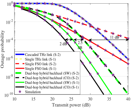
(a)

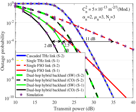
(b)

Figure 9: Comparison of outage probability for both system models versus transmit power.

In Fig. 8(a), we show the movement of the UE in between the donor and the middle IAB nodes and its impact on the E2E outage performance. We consider that the UE is at distance $d$ apart from the donor IAB node and is moving towards the middle IAB node. We consider the cases when the donor IAB is serving the UE directly, when the middle IAB node is serving the UE via 200m hybrid THz/FSO link (System-1 (second case of Fig. 8(a))), or the middle IAB node is serving the UE via 200 m THz link (System-2 (third case of Fig. 8(a))).

From Fig. 8(c), we observe that the outage performance at the UE is low till 100 m when it is served by the donor IAB directly. However, with further increase in $d$, the UE reaches in the middle IAB’s coverage region. Hence, the performance decreases rapidly when donor IAB serves the UE. At the same time, it receives strong signal for the middle IAB node, and has improved performance, compared to the case when the UE is served by the donor IAB node. Hence, there exist a handover after 100 m distance, and the UE is served by the middle IAB node, while the UE was earlier served by the donor IAB node. Further, we have better performance with System-1 (with hybrid THz/FSO link) as compared to System-2 (with single THz link) when the middle IAB serves the UE. Finally, Fig. 8(c) shows the same impact of the jitter standard deviation $\varepsilon$ on the 200 m hybrid THz/FSO link (System-1) and the 200 m THz link (System-2) between the donor IAB and the middle IAB nodes, as also discussed in Fig. 7(c).

Considering 10 UEs associated to each IAB node with $\mathcal{R}=0.1$ bps/Hz, we set the threshold at each IAB and obtain the outage results for both systems with switching/combining methods in Fig. 9. Here, Fig. 9(a) and Fig. 9(b) show the results for the strong and moderate turbulence/fading, respectively. From Fig. 9(a), we observe that the FSO link of System-1 has significant performance improvement (around 11 dB for an outage probability $10^{-4}$) than the FSO link of System-2. This allows superior outage performance for System-1, as compared to System-2 for both switching/combining methods (around 2.5 dB gain with switching and 4.5 dB gain with combining method for an outage probability $10^{-4}$). Also, the combining method provides around 2 dB gain over the switching method for System-1. However, the outage performance remains the same for both switching/combining methods for System-2. This is because the switching/combining is performed at the second hop and the single THz link of the first hop dominates in overall performance. The similar insights can be obtained from Fig. 9(b) for the moderate turbulence/fading case.

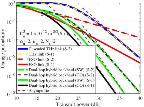
Figure 10: Theoretical and asymptotic outage probability of both the systems for combining/switching methods.

In Fig. 10, the asymptotic outage probability results are shown for both systems. The asymptotic outage results follow the exact outage probability at medium and high SNRs which validates their accuracy. Further, at high SNRs, the results of combining and switching have the same slope for both systems which justifies the same diversity order for the combining and switching methods. The diversity order of the FSO link is $\text{min}\left(\frac{\xi_{\text{F}_{n}}^{2}}{\kappa},\frac{\alpha_{\text{F}_{n}}}{\kappa},\frac{\beta_{\text{F}_{n}}}{\kappa}\right)$ and the diversity order of the THz link is $\min\left(\frac{\xi_{\text{T}_{n}}^{2}}{2},\frac{\alpha_{n}N_{\text{r}}\mu_{n}}{2}\right)$. Thus, with multi-hop parallel THz/FSO deployment, the diversity order of System-1 for both combining and switching is given by (III-B2). Similarly, the diversity order of System-2 for both the combining/switching methods is obtained by (51).

VII Conclusions

In this work, we consider multi-hop and mesh hybrid THz/FSO-based backhaul networks with different deployments of the THz and the FSO links, and analyze their performance for the cases with both IAB and non-IAB based communication setups. For the analysis, we consider both the combining and switching methods between the THz/FSO links, and the impact of various practical considerations like atmospheric attenuation/path-loss, pointing/misalignment error, atmospheric turbulence/fading, number of antennas, number of UEs, number of hops, and the threshold data-rates are shown on the performance of considered systems. From the results, we observe that the parallel deployment of the THz/FSO links in the backhaul with proper system configuration improves the overall performance of the communication system. Also, the diversity order for combining and switching methods remains the same. However, combining provides a considerable performance gain, compared to switching. Further, the increased jitter standard deviation drastically reduces the performance of the THz, the FSO, and consequently the backhaul THz/FSO link. This significantly deteriorates the E2E performance. Then, an increase in number of hops increases the coverage area, at the cost of traffic congestion and E2E latency. Finally, mesh networks enable multiple routes and improve the E2E performance significantly.

Appendix A Proof of Outage Probability for Combining Method

The (26) can be solved as

$$\mathcal{P}^{\text{ST}}_{\gamma_{\text{I}_{n}}}(\gamma_{\text{th},n})=\int_{0}^{\gamma_{\text{th},n}}f_{\gamma_{\text{F}_{n}}}(\gamma)F_{\gamma_{\text{T}_{n}}}(\gamma_{\text{th},n}-\gamma)\text{d}\gamma,$$

$$=\frac{\xi^{2}_{\text{F}_{n}}}{\kappa\Gamma(\alpha_{\text{F}_{n}})\Gamma(\beta_{\text{F}_{n}})}\frac{\mathbb{C}^{n}_{1}}{\xi_{\text{T}_{n}}^{2}}$$

$$\times\int_{0}^{\gamma_{\text{th},n}}\gamma^{-1}\text{G}^{3,0}_{1,3}\left[\frac{\alpha_{\text{F}_{n}}\beta_{\text{F}_{n}}}{A_{0{\text{F}_{n}}}\delta_{{\kappa_{n}}}^{\frac{1}{\kappa}}}\gamma^{\frac{1}{\kappa}}\Big{|}^{\xi^{2}_{\text{F}_{n}}+1}_{\xi^{2}_{\text{F}_{n}},\alpha_{\text{F}_{n}},\beta_{\text{F}_{n}}}\right]$$

$$\times\Bigg{[}\left(\frac{\gamma_{\text{th},n}-\gamma}{{\bar{\gamma}}_{\text{T}_{n}}}\right)^{\frac{\xi_{\text{T}_{n}}^{2}}{2}}\Gamma\left(\mathbb{C}^{n}_{2},\frac{\mathbb{C}^{n}_{3}}{{{\bar{\gamma}}_{\text{T}_{n}}}^{\frac{\alpha_{n}}{2}}}\left(\gamma_{\text{th},n}-\gamma\right)^{\frac{\alpha_{n}}{2}}\right)$$

$$+{\left(\mathbb{C}^{n}_{3}\right)}^{-\frac{\xi_{\text{T}_{n}}^{2}}{\alpha_{n}}}\Upsilon\left(N_{\text{r}}\mu_{n},\frac{\mathbb{C}^{n}_{3}}{{{\bar{\gamma}}_{\text{T}_{n}}}^{\frac{\alpha_{n}}{2}}}\left(\gamma_{\text{th},n}-\gamma\right)^{\frac{\alpha_{n}}{2}}\right)\Bigg{]}\text{d}\gamma.$$ (A.1)

Series expansion of the lower incomplete gamma function is given as [53, (8.354.2)]

$$\Gamma\left(a,bx\right)=\Gamma\left(a\right)- \sum_{z_{1}=0}^{\infty}\frac{(-1)^{z_{1}}}{z_{1}!\left(a+z_{1}\right)}\left(bx\right)^{a+z_{1}},$$

$$~{}~{}~{}~{}~{}~{}~{}~{}~{}~{}~{}~{}\text{for }\left[a\neq 0,-1,-2,...\right].$$ (A.2)

Substituting (A) in (A), we obtain

$$\mathcal{P}^{\text{ST}}_{\gamma_{\text{I}_{n}}}(\gamma_{\text{th},n})=\frac{\xi^{2}_{\text{F}_{n}}}{\kappa\Gamma(\alpha_{\text{F}_{n}})\Gamma(\beta_{\text{F}_{n}})}\frac{\mathbb{C}^{n}_{1}}{\xi_{\text{T}_{n}}^{2}}$$

$$\times\int_{0}^{\gamma_{\text{th},n}}\gamma^{-1}\text{G}^{3,0}_{1,3}\left[\frac{\alpha_{\text{F}_{n}}\beta_{\text{F}_{n}}}{A_{0{\text{F}_{n}}}\delta_{{\kappa_{n}}}^{\frac{1}{\kappa}}}\gamma^{\frac{1}{\kappa}}\Big{|}^{\xi^{2}_{\text{F}_{n}}+1}_{\xi^{2}_{\text{F}_{n}},\alpha_{\text{F}_{n}},\beta_{\text{F}_{n}}}\right]$$

$$\times\Bigg{[}\left(\frac{\gamma_{\text{th},n}-\gamma}{{\bar{\gamma}}_{\text{T}_{n}}}\right)^{\frac{\xi_{\text{T}_{n}}^{2}}{2}}\bigg{(}\Gamma\left(\mathbb{C}^{n}_{2}\right)-\sum_{z_{1}=0}^{\infty}\frac{(-1)^{z_{1}}}{z_{1}!\left(\mathbb{C}^{n}_{2}+z_{1}\right)}$$

$$\times\left(\frac{\mathbb{C}^{n}_{3}}{{{\bar{\gamma}}_{\text{T}_{n}}}^{\frac{\alpha_{n}}{2}}}\right)^{\mathbb{C}^{n}_{2}+z_{1}}\left(\gamma_{\text{th},n}-\gamma\right)^{\frac{\alpha_{n}}{2}\left(\mathbb{C}^{n}_{2}+z_{1}\right)}\bigg{)}$$

$$+{\left(\mathbb{C}^{n}_{3}\right)}^{-\frac{\xi_{\text{T}_{n}}^{2}}{\alpha_{n}}}\sum_{z_{1}=0}^{\infty}\frac{(-1)^{z_{1}}}{z_{1}!\left(N_{\text{r}}\mu_{n}+z_{1}\right)}\left(\frac{\mathbb{C}^{n}_{3}}{{{\bar{\gamma}}_{\text{T}_{n}}}^{\frac{\alpha_{n}}{2}}}\right)^{N_{\text{r}}\mu_{n}+z_{1}}$$

$$\times\left(\gamma_{\text{th},n}-\gamma\right)^{\frac{\alpha_{n}}{2}\left(N_{\text{r}}\mu_{n}+z_{1}\right)}\Bigg{]}\text{d}\gamma.$$ (A.3)

This can be written as

$$\mathbb{I}_{1}(\gamma_{\text{th},n})-\mathbb{I}_{2}(\gamma_{\text{th},n})+\mathbb{I}_{3}(\gamma_{\text{th},n}),$$ (A.4)

where identities $\mathbb{I}_{1}(\gamma_{\text{th},n})$, $\mathbb{I}_{2}(\gamma_{\text{th},n})$, and $\mathbb{I}_{3}(\gamma_{\text{th},n})$ are shown in (A), at the top of the next page.

$$\mathbb{I}_{1}(\gamma_{\text{th},n}) =\frac{\xi^{2}_{\text{F}_{n}}}{\kappa\Gamma(\alpha_{\text{F}_{n}})\Gamma(\beta_{\text{F}_{n}})}\frac{\mathbb{C}^{n}_{1}\Gamma\left(\mathbb{C}^{n}_{2}\right)}{\xi_{\text{T}_{n}}^{2}{{\bar{\gamma}}_{\text{T}_{n}}}^{\frac{\xi^{2}_{\text{T}}}{2}}}\int_{0}^{\gamma_{\text{th},n}}\gamma^{-1}\left(\gamma_{\text{th},n}-\gamma\right)^{\frac{\xi^{2}_{\text{T}_{n}}}{2}}\text{G}^{3,0}_{1,3}\left[\frac{\alpha_{\text{F}_{n}}\beta_{\text{F}_{n}}}{A_{0\text{F}_{n}}\delta_{\kappa_{n}}^{1/\kappa}}\gamma^{\frac{1}{\kappa}}\Big{|}^{\xi^{2}_{\text{F}_{n}}+1}_{\xi^{2}_{\text{F}_{n}},\alpha_{\text{F}_{n}},\beta_{\text{F}_{n}}}\right]\text{d}\gamma,$$

$$\mathbb{I}_{2}(\gamma_{\text{th},n}) =\frac{\xi^{2}_{\text{F}_{n}}}{\kappa\Gamma(\alpha_{\text{F}_{n}})\Gamma(\beta_{\text{F}_{n}})}\frac{\mathbb{C}^{n}_{1}}{\xi_{\text{T}_{n}}^{2}{{\bar{\gamma}}_{\text{T}_{n}}}^{\frac{\xi^{2}_{\text{T}}}{2}}}\sum_{z_{1}=0}^{\infty}\frac{(-1)^{z_{1}}}{z_{1}!\left(\mathbb{C}^{n}_{2}+z_{1}\right)}\left(\frac{\mathbb{C}^{n}_{3}}{{{\bar{\gamma}}_{\text{T}_{n}}}^{\frac{\alpha_{n}}{2}}}\right)^{\mathbb{C}^{n}_{2}+z_{1}}$$

$$\times\int_{0}^{\gamma_{\text{th},n}}\gamma^{-1}\left(\gamma_{\text{th},n}-\gamma\right)^{\frac{\xi^{2}_{\text{T}}}{2}+\frac{\alpha_{n}}{2}\left(\mathbb{C}^{n}_{2}+z_{1}\right)}\text{G}^{3,0}_{1,3}\left[\frac{\alpha_{\text{F}_{n}}\beta_{\text{F}_{n}}}{A_{0\text{F}_{n}}\delta_{\kappa_{n}}^{1/\kappa}}\gamma^{\frac{1}{\kappa}}\Big{|}^{\xi^{2}_{\text{F}_{n}}+1}_{\xi^{2}_{\text{F}_{n}},\alpha_{\text{F}_{n}},\beta_{\text{F}_{n}}}\right]\text{d}\gamma,$$

$$\mathbb{I}_{3}(\gamma_{\text{th},n}) =\frac{\xi^{2}_{\text{F}_{n}}}{\kappa\Gamma(\alpha_{\text{F}_{n}})\Gamma(\beta_{\text{F}_{n}})}\frac{\mathbb{C}^{n}_{1}{\left(\mathbb{C}^{n}_{3}\right)}^{-\frac{\xi_{\text{T}_{n}}^{2}}{\alpha}}}{\xi_{\text{T}_{n}}^{2}}\sum_{z_{2}=0}^{\infty}\frac{(-1)^{z_{2}}}{z_{2}!\left(N_{\text{r}}\mu+z_{2}\right)}\left(\frac{\mathbb{C}^{n}_{3}}{{{\bar{\gamma}}_{\text{T}_{n}}}^{\frac{\alpha_{n}}{2}}}\right)^{N_{\text{r}}\mu+z_{2}}$$

$$\times\int_{0}^{\gamma_{\text{th},n}}\gamma^{-1}\left(\gamma_{\text{th},n}-\gamma\right)^{\frac{\xi^{2}_{\text{T}}}{2}+\frac{\alpha_{n}}{2}\left(N_{\text{r}}\mu+z_{2}\right)}\text{G}^{3,0}_{1,3}\left[\frac{\alpha_{\text{F}_{n}}\beta_{\text{F}_{n}}}{A_{0\text{F}_{n}}\delta_{\kappa_{n}}^{1/\kappa}}\gamma^{\frac{1}{\kappa}}\Big{|}^{\xi^{2}_{\text{F}_{n}}+1}_{\xi^{2}_{\text{F}_{n}},\alpha_{\text{F}_{n}},\beta_{\text{F}_{n}}}\right]\text{d}\gamma.$$ (A.5)

Applying [48, (07.34.21.0085.01)] with mathematical computations, closed-form solutions of the identities $\mathbb{I}_{1}(\gamma_{\text{th},n})$, $\mathbb{I}_{2}(\gamma_{\text{th},n})$, and $\mathbb{I}_{3}(\gamma_{\text{th},n})$ are obtained as given in (III-A1).

Appendix B Proof of Diversity Analysis for Combining Method

Substituting the high SNR PDF expression of the FSO link (12) and the high SNR CDF expression of the THz link (II-B3) in (32), we obtain

$$\mathcal{P}^{\text{ST,A}}_{\gamma_{\text{I}_{n}}}(\gamma_{\text{th},n})\approx\frac{\xi^{2}_{\text{F}_{n}}}{\kappa\Gamma(\alpha_{\text{F}_{n}})\Gamma(\beta_{\text{F}_{n}})}$$

$$\times\sum_{p=1}^{3}\frac{\overset{3}{\underset{\underset{q\neq p}{q=1}}{\prod}}\Gamma(\Psi_{4,q}-\Psi_{4,p})}{\overset{1}{\underset{q=1}{\prod}}\Gamma(\Psi_{3,q}-\Psi_{4,p})}\left(\frac{\alpha_{\text{F}_{n}}\beta_{\text{F}_{n}}}{A_{0{\text{F}_{n}}}}\right)^{\Psi_{4,p}}\left(\frac{1}{\delta_{\kappa_{n}}}\right)^{\frac{\Psi_{4,p}}{\kappa}}$$

$$\times\int_{0}^{\gamma_{\text{th},n}}\gamma^{\frac{\Psi_{4,p}}{\kappa}-1}\bigg{[}\frac{\mathbb{C}^{n}_{1}\Gamma(\mathbb{C}^{n}_{2})}{\xi_{\text{T}_{n}}^{2}{{\bar{\gamma}}_{\text{T}_{n}}}^{\frac{\xi_{\text{T}_{n}}^{2}}{2}}}\left(\gamma_{\text{th},n}-\gamma\right)^{\frac{\xi_{\text{T}_{n}}^{2}}{2}}$$

$$-\frac{\mathbb{C}^{n}_{1}{\left(\mathbb{C}^{n}_{3}\right)}^{\mathbb{C}^{n}_{2}}}{\mathbb{C}^{n}_{2}\left(\alpha_{n}N_{\text{r}}\mu_{n}\right){\bar{\gamma}}_{\text{T}_{n}}^{\frac{\alpha_{n}N_{\text{r}}\mu_{n}}{2}}}\left(\gamma_{\text{th},n}-\gamma\right)^{\frac{\alpha_{n}N_{\text{r}}\mu_{n}}{2}}\bigg{]}\text{d}\gamma,$$ (B.1)

Applying the identity [53, (3.191.1)] in (B) with mathematical computations, we obtain

$$\mathcal{P}^{\text{ST,A}}_{\gamma_{\text{I}_{n}}}(\gamma_{\text{th},n})\approx\frac{\xi^{2}_{\text{F}_{n}}}{\kappa\Gamma(\alpha_{\text{F}_{n}})\Gamma(\beta_{\text{F}_{n}})}$$

$$\times\sum_{p=1}^{3}\frac{\overset{3}{\underset{\underset{q\neq p}{q=1}}{\prod}}\Gamma(\Psi_{4,q}-\Psi_{4,p})}{\overset{1}{\underset{q=1}{\prod}}\Gamma(\Psi_{3,q}-\Psi_{4,p})}\left(\frac{\alpha_{\text{F}_{n}}\beta_{\text{F}_{n}}}{A_{0{\text{F}_{n}}}}\right)^{\Psi_{4,p}}\left(\frac{1}{\delta_{\kappa_{n}}}\right)^{\frac{\Psi_{4,p}}{\kappa}}$$

$$\times\bigg{[}\frac{\mathbb{C}^{n}_{1}\Gamma(\mathbb{C}^{n}_{2})}{\xi_{\text{T}_{n}}^{2}{{\bar{\gamma}}_{\text{T}_{n}}}^{\frac{\xi_{\text{T}_{n}}^{2}}{2}}}\left(\gamma_{\text{th},n}\right)^{\frac{\xi_{\text{T}_{n}}^{2}}{2}+\frac{\Psi_{4,p}}{\kappa}}\text{B}\left(\frac{\xi_{\text{T}_{n}}^{2}}{2}+1,\frac{\Psi_{4,p}}{\kappa}\right)$$

$$-\frac{\mathbb{C}^{n}_{1}{\left(\mathbb{C}^{n}_{3}\right)}^{\mathbb{C}^{n}_{2}}}{\mathbb{C}^{n}_{2}\left(\alpha_{n}N_{\text{r}}\mu_{n}\right){\bar{\gamma}}_{\text{T}_{n}}^{\frac{\alpha_{n}N_{\text{r}}\mu_{n}}{2}}}\left(\gamma_{\text{th},n}\right)^{\frac{\alpha_{n}N_{\text{r}}\mu_{n}}{2}+\frac{\Psi_{4,p}}{\kappa}}$$

$$\times\text{B}\left(\frac{\alpha_{n}N_{\text{r}}\mu_{n}}{2}+1,\frac{\Psi_{4,p}}{\kappa}\right)\bigg{]},$$ (B.2)

where $\text{B}\left(a,b\right)=\int_{0}^{1}z^{a-1}(1-z)^{b-1}\text{d}z$ represents the Beta function.

At high SNRs, the transmit SNR $\bar{\gamma}\rightarrow\infty$. Consequently, the average received SNR of the THz and the FSO links also tend to infinity, i.e, $\bar{\gamma}_{\text{T}_{n}},\delta_{\kappa_{n}}\rightarrow\infty$. Hence, considering $\bar{\gamma}_{\text{T}_{n}}=\Delta_{1}\bar{\gamma}$ and $\delta_{\kappa_{n}}=\Delta_{2}\bar{\gamma}$, where $\Delta_{1}$ and $\Delta_{2}$ are constants, (B) can be finally simplified as (III-A2).

References

- [1] M. Agiwal, A. Roy, and N. Saxena, “Next generation 5G wireless networks: A comprehensive survey,” IEEE Commun. Surv. Tuto., vol. 18, no. 3, pp. 1617–1655, Feb. 2016.
- [2] C. Madapatha, B. Makki, C. Fang, O. Teyeb, E. Dahlman, M.-S. Alouini, and T. Svensson, “On integrated access and backhaul networks: Current status and potentials,” IEEE Open J. Commun. Soc., vol. 1, pp. 1374–1389, Sep. 2020.
- [3] C. Madapatha, B. Makki, A. Muhammad, E. Dahlman, M.-S. Alouini, and T. Svensson, “On topology optimization and routing in integrated access and backhaul networks: A genetic algorithm-based approach,” IEEE Open J. Commun. Soc., vol. 2, pp. 2273–2291, Sep. 2021.
- [4] Y. Zhang, M. A. Kishk, and M.-S. Alouini, “A survey on integrated access and backhaul networks,” Frontiers Commun. Netw., vol. 2, p. 647284, Jun. 2021.
- [5] M. N. Islam, S. Subramanian, and A. Sampath, “Integrated access backhaul in millimeter wave networks,” in Proc. IEEE WCNC’2017, San Francisco, CA, USA, Mar. 2017, pp. 1–6.
- [6] Y. Liu, A. Tang, and X. Wang, “Joint incentive and resource allocation design for user provided network under 5G integrated access and backhaul networks,” IEEE Trans. Netw. Sci. Eng., vol. 7, no. 2, pp. 673–685, Apr. 2019.
- [7] H. Yin, S. Roy, and L. Cao, “Routing and resource allocation for IAB multi-hop network in 5G advanced,” IEEE Trans. Commun., vol. 70, no. 10, pp. 6704–6717, Aug. 2022.
- [8] O. Teyeb, A. Muhammad, G. Mildh, E. Dahlman, F. Barac, and B. Makki, “Integrated access backhauled networks,” in Proc. IEEE VTC’2019, Honolulu, HI, USA, Sep. 2019, pp. 1–5.
- [9] J. Y. Lai, W.-H. Wu, and Y. T. Su, “Resource allocation and node placement in multi-hop heterogeneous integrated-access-and-backhaul networks,” IEEE Access, vol. 8, pp. 122 937–122 958, Jul. 2020.
- [10] M. Polese, M. Giordani, T. Zugno, A. Roy, S. Goyal, D. Castor, and M. Zorzi, “Integrated access and backhaul in 5G mmwave networks: Potential and challenges,” IEEE Commun. Mag., vol. 58, no. 3, pp. 62–68, Mar. 2020.
- [11] F. Gomez-Cuba and M. Zorzi, “Optimal link scheduling in millimeter wave multi-hop networks with space division multiple access,” in Proc. IEEE ITA’2016, La Jolla, CA, USA, Jan. 2016, pp. 1–9.
- [12] M. N. Kulkarni, J. G. Andrews, and A. Ghosh, “Performance of dynamic and static TDD in self-backhauled millimeter wave cellular networks,” IEEE Trans. Wireless Commun., vol. 16, no. 10, pp. 6460–6478, Jul. 2017.
- [13] B. Makki, M. Hashemi, L. Bao, and M. Coldrey, “On the performance of FDD and TDD systems in different data traffics: Finite block-length analysis,” in Proc. IEEE VTC’2018, Chicago, IL, USA, Aug. 2018, pp. 1–5.
- [14] V. F. Monteiro, F. Lima, R. Marques, D. C. Moreira, D. A. Sousa, T. F. Maciel, B. Makki, R. Shreevastav, and H. Hannu, “TDD frame design for interference handling in mobile IAB networks,” arXiv preprint arXiv:2204.13198, Apr. 2022.
- [15] V. F. Monteiro, F. R. M. Lima, D. C. Moreira, D. A. Sousa, T. F. Maciel, B. Makki, and H. Hannu, “Paving the way toward mobile IAB: Problems, solutions and challenges,” IEEE Open J. Commun. Soc., vol. 3, pp. 2347–2379, Nov. 2022.
- [16] S. Singh, M. N. Kulkarni, A. Ghosh, and J. G. Andrews, “Tractable model for rate in self-backhauled millimeter wave cellular networks,” IEEE J. Sel. Areas Commun., vol. 33, no. 10, pp. 2196–2211, May 2015.
- [17] C. Saha and H. S. Dhillon, “Millimeter wave integrated access and backhaul in 5G: Performance analysis and design insights,” IEEE J. Sel. Areas Commun., vol. 37, no. 12, pp. 2669–2684, Oct. 2019.
- [18] H. Elayan, O. Amin, B. Shihada, R. M. Shubair, and M.-S. Alouini, “Terahertz band: The last piece of RF spectrum puzzle for communication systems,” IEEE Open J. Commun. Soc., vol. 1, pp. 1–32, Nov. 2019.
- [19] N. Rajatheva, I. Atzeni, S. Bicais, E. Bjornson, A. Bourdoux, S. Buzzi, C. D’Andrea, J.-B. Dore, S. Erkucuk, M. Fuentes et al., “Scoring the terabit/s goal: Broadband connectivity in 6G,” arXiv preprint arXiv:2008.07220, Aug. 2020.
- [20] S. Li and L. Yang, “Performance analysis of dual-hop THz transmission systems over - fading channels with pointing errors,” IEEE Internet Things J., Dec. 2021.
- [21] A. Trichili, M. A. Cox, B. S. Ooi, and M.-S. Alouini, “Roadmap to free space optics,” J. Optical Society America B, vol. 37, no. 11, pp. A184–A201, Nov. 2020.
- [22] P. K. Singya and M.-S. Alouini, “Performance of UAV assisted multiuser terrestrial-satellite communication system over mixed FSO/RF channels,” IEEE Trans. Aero. Electron. Syst., vol. 58, no. 2, pp. 781–796, Sep. 2021.
- [23] P. K. Singya, N. Kumar, V. Bhatia, and M.-S. Alouini, “On the performance analysis of higher order QAM schemes over mixed RF/FSO systems,” IEEE Trans. Veh. Technol., vol. 69, no. 7, pp. 7366–7378, Apr. 2020.
- [24] B. Makki, T. Svensson, M. Brandt-Pearce, and M.-S. Alouini, “On the performance of millimeter wave-based RF-FSO multi-hop and mesh networks,” IEEE Tran. Wireless Commun., vol. 16, no. 12, pp. 7746–7759, Sep. 2017.
- [25] ——, “Performance analysis of RF-FSO multi-hop networks,” in Proc. IEEE WCNC’2017, San Francisco, CA, USA, Mar. 2017, pp. 1–6.
- [26] E. Zedini, A. Kammoun, and M.-S. Alouini, “Performance of multibeam very high throughput satellite systems based on FSO feeder links with HPA nonlinearity,” IEEE Trans. Wireless Commun., vol. 19, no. 9, pp. 5908–5923, Jun. 2020.
- [27] J.-H. Lee, K.-H. Park, Y.-C. Ko, and M.-S. Alouini, “Throughput maximization of mixed FSO/RF UAV-aided mobile relaying with a buffer,” IEEE Trans. Wireless Commun., vol. 20, no. 1, pp. 683–694, Oct. 2020.
- [28] G. Xu and Z. Song, “Performance analysis for mixed - fading and M-distribution dual-hop radio frequency/free space optical communication systems,” IEEE Trans. Wireless Commun., vol. 20, no. 3, pp. 1517–1528, Nov. 2020.
- [29] P. K. Singya and M.-S. Alouini, “Mixed FSO/RF based multiple HAPs assisted multiuser multiantenna terrestrial communication,” Frontiers Commun. Netw., Mar. 2022.
- [30] M. Z. Hassan, M. J. Hossain, J. Cheng, and V. C. Leung, “Hybrid RF/FSO backhaul networks with statistical-QoS-aware buffer-aided relaying,” IEEE Trans. Wireless Commun., vol. 19, no. 3, pp. 1464–1483, Oct. 2019.
- [31] A. Douik, H. Dahrouj, T. Y. Al-Naffouri, and M.-S. Alouini, “Hybrid radio/free-space optical design for next generation backhaul systems,” IEEE Trans. Commun., vol. 64, no. 6, pp. 2563–2577, Apr. 2016.
- [32] S. Sharma, A. Madhukumar, and R. Swaminathan, “Switching-based cooperative decode-and-forward relaying for hybrid FSO/RF networks,” IEEE/OSA J. Optical Commun. Netw., vol. 11, no. 6, pp. 267–281, Jun. 2019.
- [33] R. Swaminathan, S. Sharma, N. Vishwakarma, and A. Madhukumar, “HAPS-based relaying for integrated space-air-ground networks with hybrid FSO/RF communication: A performance analysis,” IEEE Trans. Aero. Electron. Syst., vol. 57, no. 3, pp. 1581–1599, Jan. 2021.
- [34] A. Gupta, P. Garg, and N. Sharma, “Hard switching-based hybrid RF/VLC system and its performance evaluation,” Wiley Trans. Emerg. Telecommun. Technol., vol. 30, no. 2, p. e3515, Feb. 2019.
- [35] S. Nath, S. Sengar, S. K. Shrivastava, and S. P. Singh, “Impact of atmospheric turbulence, pointing error, and traffic pattern on the performance of cognitive hybrid FSO/RF system,” IEEE Trans. Cognitive Commun. Netw., vol. 5, no. 4, pp. 1194–1207, Nov. 2019.
- [36] S. Althunibat, R. Mesleh, and K. Qaraqe, “Secure index-modulation based hybrid free space optical and millimeter wave links,” IEEE Trans. Veh.Technol., vol. 69, no. 6, pp. 6325–6332, Apr. 2020.
- [37] T. Rakia, H.-C. Yang, M.-S. Alouini, and F. Gebali, “Outage analysis of practical FSO/RF hybrid system with adaptive combining,” IEEE Commun. Lett., vol. 19, no. 8, pp. 1366–1369, Jun. 2015.
- [38] B. Makki, T. Svensson, T. Eriksson, and M.-S. Alouini, “On the performance of RF-FSO links with and without hybrid ARQ,” IEEE Trans. Wireless Commun., vol. 15, no. 7, pp. 4928–4943, Apr. 2016.
- [39] K. Nock, C. Font, and M. Rupar, “Adaptive transmission algorithms for a hard-switched FSO/RF link,” in Proc. IEEE MILCOM’2016, Baltimore, MD, USA, Dec. 2016, pp. 877–881.
- [40] A.-A. A. Boulogeorgos and A. Alexiou, “Error analysis of mixed THz-RF wireless systems,” IEEE Commun. Lett., vol. 24, no. 2, pp. 277–281, Dec. 2019.
- [41] P. Bhardwaj and S. Zafaruddin, “Performance of dual-hop relaying for THz-RF wireless link over asymmetrical fading,” IEEE Trans. Veh. Technol., vol. 70, no. 10, pp. 10 031–10 047, Jul. 2021.
- [42] S. Li, L. Yang, J. Zhang, P. S. Bithas, T. A. Tsiftsis, and M.-S. Alouini, “Mixed THz/FSO relaying systems: Statistical analysis and performance evaluation,” IEEE Trans. Wireless Commun., 2022.
- [43] P. K. Singya, B. Makki, A. D’Errico, and M.-S. Alouini, “Hybrid FSO/THz-based backhaul network for mmwave terrestrial communication,” IEEE Trans. Wireless Commun., 2022.
- [44] H. Henniger and O. Wilfert, “An introduction to free-space optical communications.” Radioengineering, vol. 19, no. 2, Jun. 2010.
- [45] A. A. Farid and S. Hranilovic, “Outage capacity optimization for free-space optical links with pointing errors,” J. Lightwave Technol., vol. 25, no. 7, pp. 1702–1710, Jul. 2007.
- [46] K.-J. Jung, S. S. Nam, M.-S. Alouini, and Y.-C. Ko, “Unified finite series approximation of FSO performance over strong turbulence combined with various pointing error conditions,” IEEE Trans. Commun., vol. 68, no. 10, pp. 6413–6425, Jul. 2020.
- [47] M. Abramowitz and I. A. Stegun, “Handbook of Mathematical Functions with Formulas, Graphs, and Mathematical Tables,” New York, NY, USA: Dover, 1972.
- [48] The Wolfram Function Site. [Online]. Available: http://functions.wolfram.com/
- [49] J. Kokkoniemi, J. Lehtomäki, and M. Juntti, “A line-of-sight channel model for the 100–450 gigahertz frequency band,” EURASIP J. Wireless Commun. Netw., vol. 2021, no. 1, pp. 1–15, Dec. 2021.
- [50] P. K. Singya, B. Makki, A. D’Errico, and M.-S. Alouini, “Hybrid FSO/THz-based backhaul network for mmwave terrestrial communication,” arXiv preprint arXiv:2204.08357, Apr. 2022.
- [51] E. N. Papasotiriou, A.-A. A. Boulogeorgos, K. Haneda, M. F. de Guzman, and A. Alexiou, “An experimentally validated fading model for THz wireless systems,” Nature Scientific Reports, vol. 11, no. 1, pp. 1–14, Sep. 2021.
- [52] B. He and R. Schober, “Bit-interleaved coded modulation for hybrid RF/FSO systems,” IEEE Trans. Commun., vol. 57, no. 12, pp. 3753–3763, Dec. 2009.
- [53] I. Gradshteyn and I. Ryzhik, Table of Integrals, Series and Products. 6th ed. New York, NY, USA: Academic, 2000.