Moving Obstacle Collision Avoidance via Chance-Constrained MPC with CBF

Abstract

Model predictive control (MPC) with control barrier functions (CBF) is a promising solution to address the moving obstacle collision avoidance (MOCA) problem. Unlike MPC with distance constraints (MPC-DC), this approach facilitates early obstacle avoidance without the need to increase prediction horizons. However, the existing MPC-CBF method is deterministic and fails to account for perception uncertainties. This paper proposes a generalized MPC-CBF approach for stochastic scenarios, which maintains the advantages of the deterministic method for addressing the MOCA problem. Specifically, the chance-constrained MPC-CBF (CC-MPC-CBF) technique is introduced to ensure that a user-defined collision avoidance probability is met by utilizing probabilistic CBFs. However, due to the potential empty intersection between the reachable set and the safe region confined by CBF constraints, the CC-MPC-CBF problem can pose challenges in achieving feasibility. To address this issue, we propose a sequential implementation approach that involves solving a standard MPC optimization problem followed by a predictive safety filter optimization, which leads to improved feasibility. Furthermore, we introduce an iterative convex optimization scheme to further expedite the resolution of the predictive safety filter, which results in an efficient approach to tackling the non-convex CC-MPC-CBF problem. We apply our proposed algorithm to a 2-D integrator system for MOCA, and we showcase its resilience to obstacle measurement uncertainties and favorable feasibility properties.

I Introduction

Moving Obstacle Collision Avoidance (MOCA) aims to enable objects to navigate safely in dynamic environments with moving obstacles. However, this critical issue presents a difficult challenge for ensuring safety in dynamic and unpredictable environments across numerous applications, including robotic arms [1], autonomous vehicles [2], and formation control [3]. To address this challenge, a range of methods have been developed, such as velocity obstacles [4], potential fields [5], and model predictive control (MPC) [6, 7, 8]. Among the various solutions, MPC is a favored approach for solving the MOCA problem due to its capability to predict the future behavior of the system and optimize a control action to satisfy safety constraints.

However, as noted in [8], the existing MOCA literature typically uses Euclidean norms for distance constraints, resulting in robots avoiding obstacles only when they are close by. The optimization process is not activated by the distance constraint until the reachable set intersects with the obstacles, meaning that a robot only takes action to avoid obstacles when it approaches them closely. This feature motivates a combination of MPC with CBF [8], which allows for avoiding obstacles in an early stage and gaining optimal performance in real-time applications. However, the MPC-CBF formulation in [8] does not account for system uncertainties, which are significant challenges frequently encountered in real-world applications. To resolve this limitation, we can modify the MPC-CBF approach to ensure robustness to uncertainties based on whether they are bounded or unbounded. For bounded uncertainties, robust CBFs [9, 10, 11], adaptive CBFs, or data-driven CBFs [12, 13] can be combined with MPC to guarantee safety under certain conditions. This can be achieved by considering the upper bounds of the uncertainties (infinity norm of the uncertainties) or estimating uncertainties with bounded estimation errors. When uncertainties are unbounded, one solution is to impose chance constraints on the safety criterion with the MPC formulation [14]. This approach ensures that the probability of collision is below a specified threshold while allowing for some violations of the constraint with a specified probability over an infinite time horizon. Another solution is to use stochastic CBFs [15] in combination with MPC, which constrains the probability of violating the CBF constraint over a finite time horizon.

In this paper, we are interested in the MOCA problem in a stochastic scenario that considers obstacle measurements with unbounded uncertainties. The contributions are three-fold:

1. We propose the CC-MPC-CBF to address the MOCA problem in a stochastic environment, which extends the (deterministic) MPC-CBF solution presented in [8]. The CC-MPC-CBF approach combines MPC with chance-constrained CBFs to handle stochastic uncertainties and provide probabilistic guarantees of safety. This approach allows for some violations of the CBF constraint with a specified probability over an infinite time horizon while ensuring that the probability of collision is below a user-specified threshold.

2. We develop a sequential implementation approach for tackling the optimization of CC-MPC-CBF to improve the feasibility, which includes two sub-optimization problems, i.e., a standard MPC and a predictive safety filter. To solve the predictive safety filter, an iterative optimization scheme is developed, which involves fixing and updating the system states iteratively while minimizing the cost function with respect to control inputs. By utilizing this methodology, we are able to obtain desirable solutions for the CC-MPC-CBF problem with improved feasibility and fast computation speed.

3. We demonstrate the effectiveness of our developed algorithms by applying them to a real MOCA example, and show their advantageous properties through numerous simulation results. Specifically, we highlight that our approach is robust to large sensing uncertainties in obstacle measurements, achieves a high success rate for MOCA, and is feasible for real-world applications.

II Preliminaries and Problem Statement

In this section, we provide an overview of the system models and definitions of discrete-time CBFs. We also examine the limitations of MPC with CBF and its inability to address system uncertainties. This motivates the chance-constrained formulation of MPC-CBF.

II-A System Models

Consider the following model governing the motion of the robot.

$$\mathbf{x}_{k+1}=\mathbf{f}(\mathbf{x}_{k})+\mathbf{g}(\mathbf{x}_{k})\mathbf{u}_{k},$$ (1)

where $\mathbf{x}_{k}\in\mathcal{X}\subset\mathbb{R}^{n}$, $\mathbf{u}_{k}\in\mathcal{U}\subset\mathbb{R}^{m}$, and the functions $\mathbf{f}:\mathbb{R}^{n}\rightarrow\mathbb{R}^{n}$ and $\mathbf{g}:\mathbb{R}^{n}\rightarrow\mathbb{R}^{n\times m}$, $m$ and $n$ are known constants. The dynamical model for an obstacle is given as:

$$\mathbf{o}_{k+1}=\bm{\xi}(\mathbf{o}_{k}),$$ (2)

where $\mathbf{o}_{k}\in\mathbb{R}^{n_{\mathrm{o}}},n_{\mathrm{o}}\leq n,$ denotes the state of the obstacle at time $k$, and $\bm{\xi}(\cdot)$ is a nonlinear state transition function.

II-B Discrete-Time Control Barrier Functions

Let a closed convex set $\mathcal{C}\subset\mathbb{R}^{n}\times\mathbb{R}^{n_{\mathrm{o}}}$ be the $0$-superlevel set of a function $h:\mathbb{R}^{n}\times\mathbb{R}^{n_{\mathrm{o}}}\rightarrow\mathbb{R}$, which is defined as

$$\mathcal{C}_{k} \triangleq\left\{(\mathbf{x}_{k},\mathbf{o}_{k})\subseteq\mathbb{R}^{n}\times\mathbb{R}^{n_{\mathrm{o}}}:h(\mathbf{x}_{k},\mathbf{o}_{k})\geq 0\right\}$$ (3)

$$\partial\mathcal{C}_{k} \triangleq\left\{(\mathbf{x}_{k},\mathbf{o}_{k})\subseteq\mathbb{R}^{n}\times\mathbb{R}^{n_{\mathrm{o}}}:h(\mathbf{x}_{k},\mathbf{o}_{k})=0\right\}$$

Herein, we assume that $\mathcal{C}_{k}$ is nonempty.

Definition 1.

(Discrete-time CBF [16]) Consider the discrete-time system (1) and (2). Given a set $\mathcal{C}_{k}$ defined by (3) for a function $h:\mathbb{R}^{n}\times\mathbb{R}^{n_{\mathrm{o}}}\rightarrow\mathbb{R}$, the function $h$ is a CBF defined on set $\mathbb{R}^{n}\times\mathbb{R}^{n_{\mathrm{o}}}$ if there exists a function $\alpha\in\mathcal{K}_{\infty}$ such that

$$\inf\limits_{\mathbf{u}\in\mathcal{U}}\Delta h(\mathbf{x}_{k},\mathbf{o}_{k},\mathbf{u}_{k})\geq-\alpha(h(\mathbf{x}_{k},\mathbf{o}_{k})),$$ (4)

where $\Delta h(\mathbf{x}_{k},\mathbf{o}_{k},\mathbf{u}_{k}):=h(\mathbf{x}_{k+1},\mathbf{o}_{k+1})-h(\mathbf{x}_{k},\mathbf{o}_{k})$.

We follow the result of [16] and select the $\mathcal{K}_{\infty}$ function $\alpha(h(\mathbf{x}_{k},\mathbf{o}_{k}))$ to be $\gamma h(\mathbf{x}_{k},\mathbf{o}_{k}),0<\gamma\leq 1$. Then the condition for CBF is defined as:

$$\mathrm{CBC}_{k}\triangleq h(\mathbf{x}_{k+1},\mathbf{o}_{k+1})-(1-\gamma)h(\mathbf{x}_{k},\mathbf{o}_{k})\geq 0,$$ (5)

where $\mathrm{CBC}_{k}=\mathrm{CBC}(\mathbf{x}_{k},\mathbf{o}_{k},\mathbf{u}_{k})$.

II-C MPC with CBF

We consider using MPC with CBF to address the MOCA problem (6). It solves the following constrained finite-time optimization control problem with horizon $N$ at each time instant $t_{k}$ with $i=0,\ldots,N-1$.

$$\min_{\mathbf{u}_{k:k+N-1\mid k}}J(\mathbf{x}_{k:k+N\mid k},\mathbf{u}_{k:k+N-1\mid k})$$ (6a)

$$\text{ s.t. }\,\mathbf{x}_{k+i+1\mid k}=\mathbf{f}(\mathbf{x}_{k+i\mid k})+\mathbf{g}(\mathbf{x}_{k+i\mid k})\mathbf{u}_{k+i\mid k},$$ (6b)

$$\qquad\mathbf{x}_{k+i\mid k}\in\mathcal{X},\quad\mathbf{u}_{k+i\mid k}\in\mathcal{U},$$ (6c)

$$\qquad\mathbf{x}_{k\mid k}=\mathbf{x}_{k},\quad\,\,\,\,\mathbf{x}_{k+N\mid k}\in\mathcal{X}_{f},$$ (6d)

$$\qquad\mathrm{CBC}_{k+i|k}\geq 0,$$ (6e)

where the cost function in (6a) is the sum of the terminal cost $p\left(\mathbf{x}_{k+N\mid k}\right)$ and stage cost $\sum_{i=0}^{N-1}q\left(\mathbf{x}_{k+i\mid k},\mathbf{u}_{k+i\mid k}\right)$, which means that $J(\mathbf{x}_{k:k+N\mid k},\mathbf{u}_{k:k+N-1\mid k})=p\left(\mathbf{x}_{k+N\mid k}\right)+\sum_{i=0}^{N-1}q\left(\mathbf{x}_{k+i\mid k},\mathbf{u}_{k+i\mid k}\right)$; (6b) describes the system dynamics; (6c) shows the state and input constraints along the horizon; and (6d) provides the constraints on initial condition and terminal set $\mathcal{X}_{f}$. The CBF constraint $\mathrm{CBC}_{k+i|k}=h\left(\mathbf{x}_{k+i+1\mid k},\mathbf{o}_{k+i+1\mid k}\right)-(1-\gamma)h\left(\mathbf{x}_{k+i\mid k},\mathbf{o}_{k+i\mid k}\right)\geq 0$ given in (6e) guarantees the forward invariance of the safety set $\mathcal{C}_{k+i|k}$ as defined in (3).

II-D Problem Statement

Due to inaccurate localization or sensing, perfect measurements of the obstacle are unavailable. We assume that the measurements of the obstacle are corrupted by stochastic noise $\bm{\omega}_{k}$ and are generated with the following model.

$$\begin{split}\mathbf{o}_{k+1}=\bm{\xi}(\mathbf{o}_{k})+\bm{\omega}_{k},\end{split}$$ (7)

where $\bm{\omega}_{k}$ is white driving noise, which follows a Gaussian distribution $\mathcal{N}(\mathbf{0},\sigma^{2}\mathbf{I}_{n_{\mathrm{o}}\times n_{\mathrm{o}}})$, where $\sigma$ is the standard deviation of the noise. Since the stochastic noise is introduced in (7), the condition in (6e) cannot be satisfied anymore. To address this issue, we are interested in modifying the MPC-CBF in (6) to handle stochastic uncertainties. Therefore, the research problem of this paper is formally stated as follows.

Problem 1.

Develop a new MPC-CBF formulation to address the MOCA problem in a stochastic environment, which allows designing a controller that is robust to the random noise in (7).

III Chance Constrained MPC-CBF

In this section, we formulate the CC-MPC-CBF to handle the influence of stochasticity that arises from noisy obstacle measurements. Specifically, we assume that the uncertainty in an obstacle measurement follows a Gaussian distribution, and we transform the chance constraint into a deterministic constraint with their mean and variance. By following the formulation in (6), the CC-MPC-CBF is provided.

III-A CBF and Chance Constraints

Hyperellipsoid is one popular choice of a discrete-time CBF and is commonly used for representing obstacles (or the region of operation where the robot is allowed to move). In our formulation, we continue to use hyperellipsoids to parameterize CBFs, which are denoted as:

$$\begin{split}h(\mathbf{x}_{k},\mathbf{o}_{k})=\|\mathbf{x}_{k}-\mathbf{o}_{k}\|_{\mathbf{W}}^{2}-1,\end{split}$$ (8)

where $\mathbf{W}\in\mathbb{R}^{n_{\mathrm{o}}\times n_{\mathrm{o}}}$ is a symmetric positive definite matrix and $\|\mathbf{x}_{k}-\mathbf{o}_{k}\|_{\mathbf{W}}^{2}=(\mathbf{x}_{k}-\mathbf{o}_{k})^{\top}\mathbf{W}(\mathbf{x}_{k}-\mathbf{o}_{k})$. It should be noted that in the equation (8), we assumed that the dimension of $\mathbf{x}_{k}$ is $n_{\mathrm{o}}$. However, when the dimension of $\mathbf{x}_{k}$ is greater than $n_{\mathrm{o}}$, the variables in (8) should correspond to a partial state of $\mathbf{x}_{k}$, rather than the full state.

Due to the stochastic noise in (7), we consider the chance-constrained optimization problem to accommodate uncertainty with $\delta\in(0,1)$ as the desired confidence of probabilistic safety. Then the chance constraint for collision avoidance is given as follows.

$$\begin{split}\mathbb{P}(\mathrm{CBC}_{k+i|k}\geq\zeta|\mathbf{x}_{k+i|k},\mathbf{o}_{k+i|k},\mathbf{u}_{k+i|k})\geq\delta,\end{split}$$ (9)

where $\mathbb{P}(\cdot)$ denotes the probability of a condition to be true, the value of $\zeta,\delta\in\mathbb{R}^{+}$ are defined by users which vary for different requirements. Herein, $\delta$ indicates the collision avoidance probability.

Note that $\mathrm{CBC}_{k+i|k}=\|\mathbf{x}_{k+i+1\mid k}-\bm{\xi}(\mathbf{o}_{k+i|k})\|_{\mathbf{W}}^{2}+\bm{\omega}_{k+i|k}^{\top}\mathbf{W}\bm{\omega}_{k+i|k}+2(\mathbf{x}_{k+i+1\mid k}-\bm{\xi}(\mathbf{o}_{k+i|k}))^{\top}\mathbf{W}\bm{\omega}_{k+i|k}-(1-\gamma)h\left(\mathbf{x}_{k+i\mid k},\mathbf{o}_{k+i\mid k}\right)-1$ does not follow a Gaussian distribution. This is due to that there exists a non-Gaussian term $\bm{\omega}_{k+i|k}^{\top}\bm{\omega}_{k+i|k}+2(\mathbf{x}_{k+i+1\mid k}-\bm{\xi}(\mathbf{o}_{k+i|k}))^{\top}\bm{\omega}_{k+i|k}$ in $\mathrm{CBC}_{k+i|k}$. However, as pointed out in [17], the non-Gaussian probability density function resulting from squaring a Gaussian random variable can be well approximated by the Gaussian density function by matching the first-order and second-order moments.

Lemma 1.

([18]) Let $\mathbf{z}$ be a Gaussian variable, and the mean value and covariance are $\bm{\mu}$ and $\bm{\Sigma}$, respectively. $\mathbf{A}$ is a symmetric matrix. Then the expectation and variance of the quadratic form $\mathbf{z}^{\top}\mathbf{A}\mathbf{z}$ are given as follows.

$$\begin{split}\mathbb{E}[\mathbf{z}^{\top}\mathbf{A}\mathbf{z}]&=\mathrm{Tr}(\mathbf{A}\bm{\Sigma})+\bm{\mu}^{\top}\mathbf{A}\bm{\mu},\\ \mathbf{Var}[\mathbf{z}^{\top}\mathbf{A}\mathbf{z}]&=2\operatorname{Tr}(\mathbf{A}\bm{\Sigma}\mathbf{A}\bm{\Sigma})+4\bm{\mu}^{\top}\mathbf{A}\bm{\Sigma}\mathbf{A}\bm{\mu},\end{split}$$ (10)

where $\mathbb{E}(\cdot)$ and $\mathbf{Var}(\cdot)$ denote the operations for computing the expectation and variance of a variable, respectively.

Corollary 1.

Consider the model (1) and (7). We approximate $\mathrm{CBC}_{k+i|k}$ using a Gaussian density, where the parameters, i.e., its expectation and variance, are given as follows.

$$\begin{split}\mathbb{E}\left[\mathrm{CBC}_{k+i|k}\right]&=\mathbf{u}_{k+i|k}^{\top}\bm{\Phi}(\mathbf{x}_{k+i|k})\mathbf{u}_{k+i|k}\\ &\quad+2\mathbf{m}^{\top}(\mathbf{x}_{k+i|k})\mathbf{u}_{k+i|k}+s(\mathbf{x}_{k+i|k})\\ \mathbf{Var}\left[\mathrm{CBC}_{k+i|k}\right]&=\mathbf{u}_{k+i|k}^{\top}\mathbf{H}(\mathbf{x}_{k+i|k})\mathbf{u}_{k+i|k}\\ &\quad+2\mathbf{n}(\mathbf{x}_{k+i|k})^{\top}\mathbf{u}_{k+i|k}+d(\mathbf{x}_{k+i|k}),\end{split}$$ (11)

where

$$\begin{split}\bm{\Phi}(\mathbf{x}_{k+i|k})&=\mathbf{g}(\mathbf{x}_{k+i|k})^{\top}\mathbf{W}\mathbf{g}(\mathbf{x}_{k+i|k})\\ \mathbf{H}(\mathbf{x}_{k+i|k})&=4\sigma^{2}\mathbf{g}(\mathbf{x}_{k+i|k})^{\top}\mathbf{W}^{\top}\mathbf{W}\mathbf{g}(\mathbf{x}_{k+i|k})\\ \mathbf{m}(\mathbf{x}_{k+i|k})&=\mathbf{g}(\mathbf{x}_{k+i|k})^{\top}\mathbf{W}(\mathbf{f}(\mathbf{x}_{k+i|k})-\bm{\xi}(\mathbf{o}_{k+i|k}))\\ \mathbf{n}(\mathbf{x}_{k+i|k})&=4\sigma^{2}\mathbf{g}(\mathbf{x}_{k+i|k})^{\top}\mathbf{W}^{\top}\mathbf{W}(\mathbf{f}(\mathbf{x}_{k+i|k})-\bm{\xi}(\mathbf{o}_{k+i|k}))\\ s(\mathbf{x}_{k+i|k})&=\|\mathbf{f}(\mathbf{x}_{k+i|k})-\bm{\xi}(\mathbf{o}_{k+i|k})\|_{\mathbf{W}}^{2}+\sigma^{2}\mathrm{tr}(\mathbf{W})\\ &-(1-\gamma)h\left(\mathbf{x}_{k+i\mid k},\mathbf{o}_{k+i\mid k}\right)-1\\ d(\mathbf{x}_{k+i|k})&=4\|\sigma\mathbf{W}(\mathbf{f}(\mathbf{x}_{k+i|k})-\bm{\xi}(\mathbf{o}_{k+i|k}))\|^{2}\\ &\quad+2\sigma^{4}\mathrm{tr}(\mathbf{W}^{\top}\mathbf{W}).\end{split}$$

Proof.

Combining the results in (5),  (6e),  (7), (8), we have

$$\begin{split}\mathrm{CBC}_{k+i|k}=&\|\mathbf{f}(\mathbf{x}_{k+i|k})+\mathbf{g}(\mathbf{x}_{k+i|k})\mathbf{u}_{k+i|k}-\bm{\xi}(\mathbf{o}_{k+i|k})\|_{\mathbf{W}}^{2}\\ &+\bm{\omega}_{k+i|k}^{\top}\mathbf{W}\bm{\omega}_{k+i|k}+2(\mathbf{f}(\mathbf{x}_{k+i|k})\\ &+\mathbf{g}(\mathbf{x}_{k+i|k})\mathbf{u}_{k+i|k}-\bm{\xi}(\mathbf{o}_{k+i|k}))^{\top}\mathbf{W}\bm{\omega}_{k+i|k}\\ &-(1-\gamma)h\left(\mathbf{x}_{k+i\mid k},\mathbf{o}_{k+i\mid k}\right)-1\end{split}$$

Next, with the use of Lemma 1, we obtain the following result.

$$\begin{split}&\mathbb{E}\left[\mathrm{CBC}_{k+i|k}\right]=\|\mathbf{f}(\mathbf{x}_{k+i|k})+\mathbf{g}(\mathbf{x}_{k+i|k})\mathbf{u}_{k+i|k}-\bm{\xi}(\mathbf{o}_{k+i|k})\|_{\mathbf{W}}^{2}\\ &\quad+\sigma^{2}\mathrm{tr}(\mathbf{W})-(1-\gamma)h\left(\mathbf{x}_{k+i\mid k},\mathbf{o}_{k+i\mid k}\right)\big{)}-1\\ &\mathbf{Var}\left[\mathrm{CBC}_{k+i|k}\right]=4\|\sigma\mathbf{W}(\mathbf{f}(\mathbf{x}_{k+i|k})+\mathbf{g}(\mathbf{x}_{k+i|k})\mathbf{u}_{k+i|k}\\ &\qquad-\bm{\xi}(\mathbf{o}_{k+i|k}))\|^{2}+2\sigma^{4}\mathrm{tr}(\mathbf{W}^{\top}\mathbf{W}).\end{split}$$ (12)

Finally, the equalities of  (11) are obtained by expanding the results regarding $\mathbf{u}_{k+i|k}$ as the variable. ∎

III-B Linear Chance Constraints

Lemma 2.

([19]) Given any vector $\mathbf{a}$ and scalar $b$, for a multivariate random variable $\mathbf{z}\in\mathcal{N}(\bm{\mu},\bm{\Sigma})$, then the linear chance constraint

$$\begin{split}\mathbb{P}\left(\mathbf{a}^{\top}\mathbf{z}\leq b\right)\leq\lambda\end{split}$$ (13)

is equivalent to a deterministic constraint

$$\begin{split}\mathbf{a}^{\top}\bm{\mu}-b\geq c,\end{split}$$ (14)

where $c=\mathrm{erf}^{-1}(1-2\lambda)\sqrt{2\mathbf{a}^{\top}\bm{\Sigma}\mathbf{a}}$, $\mathrm{erf}$ is the standard error function and is defined as $\mathrm{erf}(x)=\frac{2}{\sqrt{\pi}}\int\nolimits_{0}^{x}e^{-t^{2}}dt$, and $\lambda>0$ is a use-defined probability.

Note that the error function and its inverse corresponding to the confidence level can be obtained through table look-up or series approximation techniques. To ensure that the collision probability is below a certain threshold $1-\delta$, we derive the constraint $\mathbb{P}(\mathrm{CBC}_{k+i|k}<\zeta|\mathbf{x}_{k+i|k},\mathbf{o}_{k+i|k},\mathbf{u}_{k+i|k})<1-\delta$ from the expression in (9). By setting $\mathbf{a}=1$, $\mathbf{z}=\mathrm{CBC}_{k+i|k}$, $b=\zeta$, and $\lambda=1-\delta$ in Lemma 1, we obtain the chance constraint (9) into the following form.

$$\begin{split}\mathbb{E}\left[\mathrm{CBC}_{k+i|k}\right]-\zeta\geq c(\delta)\sqrt{\mathbf{Var}\left[\mathrm{CBC}_{k+i|k}\right]},\end{split}$$ (15)

where $c(\delta)=\sqrt{2}\mathrm{erf}^{-1}(2\delta-1)$. Substituting (11) into (15) gives the following result

$$\begin{split}&c(\delta)\sqrt{\mathbf{u}_{k+i|k}^{\top}\mathbf{H}(\mathbf{x}_{k+i|k})\mathbf{u}_{k+i|k}+2\mathbf{n}(\mathbf{x}_{k+i|k})\mathbf{u}_{k+i|k}+d(\mathbf{x}_{k+i|k})}\\ &-(\mathbf{u}_{k+i|k}^{\top}\bm{\Phi}(\mathbf{x}_{k+i|k})\mathbf{u}_{k+i|k}+2\mathbf{m}(\mathbf{x}_{k+i|k})\mathbf{u}_{k+i|k}+s(\mathbf{x}_{k+i|k}))\\ &\leq-\zeta.\end{split}$$ (16)

Remark 1.

If the measurement given in (7) is noise-free (i.e., $\sigma=0$), the variance obtained in (11) will yield $\mathbb{E}\left[\mathrm{CBC}_{k+i|k}\right]=\|\mathbf{f}(\mathbf{x}_{k+i|k})+\mathbf{g}(\mathbf{x}_{k+i|k})\mathbf{u}_{k+i|k}-\bm{\xi}(\mathbf{o}_{k+i|k})\|_{\mathbf{W}}^{2}-(1-\gamma)h\left(\mathbf{x}_{k+i\mid k},\mathbf{o}_{k+i\mid k}\right)-1$ and $\mathbf{Var}\left[\mathrm{CBC}_{k+i|k}\right]=0$. Consequently, the inequality constraint in (16) can be reduced to a deterministic constraint, i.e., (6e). Furthermore, when the prediction horizon is chosen as $N=1$, the inequality condition (16), presented below, becomes convex.

$$\begin{split}&(\mathbf{u}_{k}^{\top}\bm{\Phi}(\mathbf{x}_{k})\mathbf{u}_{k}+2\mathbf{m}(\mathbf{x}_{k})\mathbf{u}_{k}+s(\mathbf{x}_{k}))\\ &\quad-c(\delta)\sqrt{\mathbf{u}_{k}^{\top}\mathbf{H}(\mathbf{x}_{k})\mathbf{u}_{k}+2\mathbf{n}(\mathbf{x}_{k})\mathbf{u}_{k}+d(\mathbf{x}_{k})}\geq\zeta.\end{split}$$ (17)

This is due to that the state-dependent matrices, which include $\bm{\Phi}(\mathbf{x}_{k})$, $\mathbf{H}(\mathbf{x}_{k})$, $\mathbf{m}(\mathbf{x}_{k})$, $\mathbf{n}(\mathbf{x}_{k})$, $d(\mathbf{x}_{k})$, and $s(\mathbf{x}_{k})$, are constant at each time step $k$, given that $\mathbf{x}_{k}=\mathbf{x}_{k|k}$ can be measured or obtained at time $k$. Note that $\bm{\Phi}(\mathbf{x}_{k})$ and $\mathbf{H}(\mathbf{x}_{k})$ are both positive definite if $\mathbf{g}(\mathbf{x}_{k})$ is row full rank and $\mathbf{W}$ is a full rank matrix.

III-C Chance-Constrained MPC-CBF

For the MPC-CBF formulation given in (6), we usually set the terminal cost to be $p\left(\mathbf{x}_{k+N\mid k}\right)=\|\mathbf{x}_{k+N\mid k}\|_{\mathbf{P}}^{2}$ and the stage cost as $q\left(\mathbf{x}_{k+i\mid k},\mathbf{u}_{k+i\mid k}\right)=\|\mathbf{x}_{k+i\mid k}\|_{\mathbf{Q}}^{2}+\|\mathbf{u}_{k+i\mid k}\|_{\mathbf{R}}^{2}$, where $\mathbf{P}$, $\mathbf{Q}$, and $\mathbf{R}$ are positive definite weight matrices for the terminal states, stage states, and control inputs. Then the CC-MPC-CBF is formulated as follows.

$$\begin{split}&\min_{\mathbf{u}_{k:k+N-1\mid k}}p\left(\mathbf{x}_{k+N\mid k}\right)+\sum\limits_{i=1}^{N-1}q\left(\mathbf{x}_{k+i\mid k},\mathbf{u}_{k+i\mid k}\right)\\ &\quad\text{ s.t. }\eqref{Zb},\eqref{Zc},\eqref{Zd},\eqref{Re_organize},\end{split}$$ (18)

There are several off-the-shelf solvers, such as IPOPT, MOSEK, and CPLEX, that can be used to solve the non-convex optimization problem (18). Additionally, it is important to note that the terminal cost can be treated as a control Lyapunov function (CLF) and formulated as a constraint, similar to [20]. Then the formulation in (18) can be viewed as a chance-constrained MPC-CLF-CBF.

Remark 2.

The nice properties of deterministic MPC-CBF, such as avoiding obstacles at an early stage, are maintained in a stochastic scenario because the chance-constrained approach still considers the CBF constraints in the optimization problem. The chance constraint only adds an additional constraint on the probability of violating the CBF constraint.

Remark 3.

The major limitation associated with the CC-MPC-CBF approach is feasibility. Define the reachable set $\mathcal{R}_{k+i|k}=\{\mathbf{x}_{k+i|k}\in\mathbb{R}^{n}:\eqref{Zb},\eqref{Zc},\eqref{Zd}\},i=0,\cdots,N$ and safety set $\mathcal{S}_{k+i|k}=\{\mathbf{x}_{k+i|k}\in\mathbb{R}^{n}:\eqref{Re_organize}\}$. The CC-MPC-CBF (18) requires the intersection set $\mathcal{R}_{k+i|k}\cap\mathcal{S}_{k+i|k}$ is not empty, making the optimization problem possibly infeasible.

Proposition 1.

If $\delta\geq\frac{1+\mathrm{erf}(0.5)}{2}$, then introducing more randomness to the system by increasing the standard deviation of the noise $\sigma$ may lead to (18) becoming infeasible.

Proof.

The expectation and variance of $\mathrm{CBC}_{k+i|k}$ are given in (12), and $\mathbf{Var}\left[\mathrm{CBC}_{k+i|k}\right]\geq 2\sigma^{4}\mathrm{tr}(\mathbf{W}^{\top}\mathbf{W})$. Meantime, we recall the trace inequality $\sqrt{\mathrm{tr}(\mathbf{W}^{\top}\mathbf{W})}\leq\mathrm{tr}(\mathbf{W})$ with $\mathbf{W}$ being a symmetric positive definite matrix. By substituting (12) and the two inequality conditions into (15), it gives

$$\begin{split}&\mathbb{E}\left[\mathrm{CBC}_{k+i|k}\right]-c(\delta)\sqrt{\mathbf{Var}\left[\mathrm{CBC}_{k+i|k}\right]}-\zeta\\ &\leq\mathbf{D}+\sigma^{2}\mathrm{tr}(\mathbf{W})-c(\delta)\sqrt{2\sigma^{4}\mathrm{tr}(\mathbf{W}^{\top}\mathbf{W})}-\zeta\\ &\leq\mathbf{D}-\zeta+\left(1-\sqrt{2}c(\delta)\right)\sqrt{\mathrm{tr}(\mathbf{W}^{\top}\mathbf{W})}\sigma^{2},\end{split}$$ (19)

where $\mathbf{D}=\|\mathbf{f}(\mathbf{x}_{k+i|k})+\mathbf{g}(\mathbf{x}_{k+i|k})\mathbf{u}_{k+i|k}-\bm{\xi}(\mathbf{o}_{k+i|k})\|_{\mathbf{W}}^{2}-(1-\gamma)h\left(\mathbf{x}_{k+i\mid k},\mathbf{o}_{k+i\mid k}\right)\big{)}-1$ is deterministic if $\mathbf{x}_{k+i|k}$, $\mathbf{o}_{k+i|k}$, and $\mathbf{u}_{k+i|k}$ are given. We can infer that $1-\sqrt{2}c(\delta)\leq 0$, given that $\delta\geq\frac{1+\mathrm{erf}(0.5)}{2}$. This implies that an increase in $\sigma$ leads to a decrease in the safety margin defined by the inequality (15). Consequently, the size of the safety set $\mathcal{S}_{k+i|k}$ decreases, which leads to a reduction in the size of the feasible set $\mathcal{R}_{k+i|k}\cap\mathcal{S}_{k+i|k}$. Therefore, the probability of the constrained MPC in (18) being feasible also decreases. ∎

Proposition 1 highlights that the feasibility of (18) depends on the specified collision avoidance probability $\delta$. This is because the trade-off between robustness to stochasticity and feasibility cannot be simultaneously achieved in (18). For instance, when the collision avoidance probability $\delta$ is set to be high and the noise is highly stochastic, a conservative control strategy may be required to ensure safety, which may render (18) infeasible. Conversely, when a small value of $\delta$ is chosen, allowing for some level of failure in collision avoidance, the optimization problem (18) remains feasible even in the presence of high noise variability.

Remark 4.

The feasibility of (16) is influenced by the parameter $\gamma$, which has the same impact in both deterministic [8] and non-deterministic scenarios. As $\gamma$ is decreased, the parameter $s(\mathbf{x}_{k+i|k})$ defined in (11) is reduced, leading to a corresponding decrease in the expectation $\mathbb{E}\left[\mathrm{CBC}_{k+i|k}\right]$ associated with $s(\mathbf{x}_{k+i|k})$. We rewrite (15) as $c(\delta)\sqrt{\mathbf{Var}\left[\mathrm{CBC}_{k+i|k}\right]}+\zeta\leq\mathbb{E}\left[\mathrm{CBC}_{k+i|k}\right]$, which shows that the upper bound of the inequality, i.e., $\mathbb{E}\left[\mathrm{CBC}_{k+i|k}\right]$, is decreased. Consequently, as $\mathbb{E}\left[\mathrm{CBC}_{k+i|k}\right]$ decreases, the safety set $\mathcal{S}_{k+i|k}$ becomes smaller, resulting in a smaller feasible set $\mathcal{R}_{k+i|k}\cap\mathcal{S}_{k+i|k}$. Therefore, the probability of (18) being feasible will be decreased with a decrease of $\gamma$. Moreover, when $\gamma=1$, the chance-constrained CBF (9) reduces to the form $\mathbb{P}(h(\mathbf{x}_{k+i|k},\mathbf{o}_{k+i|k})\geq\zeta|\mathbf{x}_{k+i|k},\mathbf{o}_{k+i|k},\mathbf{u}_{k+i|k})\geq\delta$, which is recognized as a CC-MPC with distance constraints (CC-MPC-DC) [14].

Remark 5.

Increasing the prediction horizon is likely to raise the probability of infeasibility. This is because the introduction of more constraints, resulting from an increase in the value of $N$, will cause both sets $\mathcal{R}_{k+i|k},i=0,\cdots,N$ and $\mathcal{S}_{k+i|k}$ to contract. It may result in an empty set of $\mathcal{R}_{k+i|k}\cap\mathcal{S}_{k+i|k}$.

IV CC-MPC-CBF with a Sequential Implementation

In this section, we present a solution to address the limitation outlined in Remark 3. Specifically, we propose a sequential implementation of the CC-MPC-CBF approach. This involves decomposing (18) into two sub-optimization problems. The first sub-optimization problem utilizes the MPC formulation without CBF constraints, resulting in a standard MPC formulation. Its objective is to provide a nominal control input $\mathbf{u}_{k:k+N-1\mid k}^{\mathrm{nom}}$ that guarantees system performance, such as closed-loop stability. In the second sub-optimization problem, we ensure safety by incorporating the CBF constraints. It is formulated as follows, and we call it a predictive safety filter.

$$\begin{split}&\min_{\mathbf{u}_{k:k+N-1\mid k}}\sum\limits_{i=1}^{N-1}\|\mathbf{u}_{k+i\mid k}-\mathbf{u}_{k+i\mid k}^{\mathrm{nom}}\|_{\mathbf{R}}^{2}\\ &\quad\text{ s.t. }\quad\eqref{Re_organize}.\end{split}$$ (20)

The first sub-optimization problem has been well-studied in many existing pieces of literature [21, 22], which can be used for stabilization and reference trajectory tracking applications. For the second sub-optimization problem, it is based on the idea of the safety filter, or an active set invariance filter [23], where the nominal control input is filtered through (20) with safety guarantees because of (16). Additionally, it is noteworthy to mention that splitting (18) into a standard MPC and (20) could be a natural option for numerous applications. In real-world systems, a standard MPC is formulated without considering safety constraints, making it a preferred scenario to introduce (20).

Remark 6.

The advantage of using a sequential implementation scheme lies in the fact that the requirements ensured by the standard MPC and CBF constraints are decoupled. Consequently, the resulting optimization problem is often less restrictive than if the safety constraints were directly incorporated into the MPC formulation. In particular, in our formulation, the feasible sets for a standard MPC and a predictive safety filter are $\mathcal{R}_{k+i|k}$ and $\mathcal{S}_{k+i|k}$ respectively. Compared to the feasible region $\mathcal{R}_{k+i|k}\cap\mathcal{S}_{k+i|k}$, the feasible set of both sub-optimization problems is larger. Therefore, both of the sub-optimization problems have a lower likelihood of encountering infeasible cases compared to (18). However, this advantage comes at the cost of potentially sacrificing some degree of optimality since the safety filter modifies the nominal control input generated by MPC.

Remark 7.

In the special case that $N=1$ in (20), it is corresponding to the well-known safety filter, as detailed in [23]. However, despite its widespread recognition, this filter comes with a drawback: it sacrifices its ability to make predictions and may cause excessively aggressive behavior.

IV-A Iterative Convex Optimization

As mentioned, the first sub-optimization problem has already been extensively studied, and hence we will not provide any further descriptions in this paper. However, it is interesting to have some discussions on the second sub-optimization problem (20).

We notice that the optimization problem (20) is convex if a specific set of $\mathbf{x}_{k:k+N|k}$ are previously given, which has already been discussed in Remark 1. Therefore, we suggest using an iterative convex optimization algorithm, as outlined in Algorithm 1, to solve  (20). The proposed algorithm aims to solve (20) using a sequence of convex optimization problems in an iterative manner. In particular, the system state $\mathbf{x}_{k:k+N|k}$ of (20) is fixed and updated at each iteration while the control input is treated as the decision variable. By applying a suitable stop criterion, we can obtain a near-optimal solution of (20). Note that the variable $j$ represents the iteration number, which ranges from 1 to $j_{\mathrm{max}}$, where $j_{\mathrm{max}}$ is the maximum number of allowed iterations. The overall duration of the time interval under consideration is denoted by $k_{\mathrm{max}}$. The stop criterion at each $k$ is given as follows.

$$\sum\limits_{i=0}^{N}\|\mathbf{x}_{k+i|k}^{j+1}-\mathbf{x}_{k+i|k}^{j}\|\leq\varepsilon,$$ (21)

where $\varepsilon>0$ is constant, which can be obtained after some offline trials. It is worth noting that a weighting matrix can be included in the criterion (21). However, for simplicity, we have not taken it into account in this case. Additionally, it should be noted that we make the assumption that the starting state $\mathbf{x}_{0}$ does not encounter any obstacles and that the robot has the capability to reach the state $\mathbf{x}_{k+1|k}^{*}$ (obtained in Step 10 of Algorithm 1) before $k+1$.

0:  The system model (1) and obstacle model (7),

      state $\mathbf{x}_{k}$ at each $k,k=0,\cdots,k_{\mathrm{max}}$.

0:  Closed-loop trajectory $\mathbf{x}_{k:k+N|k}^{*}$ at each $k$.

1:  Set $k=0$ and initial guess $\mathbf{u}_{0:N-1|0}^{0}=\mathbf{u}_{k:k+N-1\mid k}^{\mathrm{nom}}$.

2:  Initialize the variables $\mathbf{x}_{0:N|0}^{0}$ using $\mathbf{x}_{0}$ and $\mathbf{u}_{0:N-1|0}^{0}$ via (6b).

3:  for $k<k_{\mathrm{max}}$ do

4:      Set $j=0$.

5:      While $j<j_{\mathrm{max}}$ or (21) is not satisfied do

6:        Fix $\mathbf{x}_{k:k+N|k}^{j}$ and compute the optimal solution

      $\mathbf{u}_{k:k+N-1|k}^{j+1}$ in (20) through some convex solvers

      like CVXOPT and GUROBI.

7:        Update the variables $\mathbf{x}_{k:k+N|k}^{j+1}$ for the next

      iteration using $\mathbf{x}_{k}$ and $\mathbf{u}_{k:k+N-1|k}^{j+1}$ via (6b).

8:        $j=j+1$.

9:      end while

10:  Extract optimized states $\mathbf{x}_{k:k+N|k}^{*}=\mathbf{x}_{k:k+N|k}^{j}$ and inputs $\mathbf{u}_{k:k+N-1|k}^{*}=\mathbf{u}_{k:k+N-1|k}^{j}$ from the last iteration.

11:  Update $\mathbf{u}_{k+1:k+N|k+1}^{0}$ with $\mathbf{u}_{k:k+N-1|k}^{*}$ and obtain the states $\mathbf{x}_{k+1:k+N+1|k+1}^{0}$ for the next time instant with $\mathbf{x}_{k}$ and $\mathbf{u}_{k:k+N-1|k}^{*}$ according to (6b).

12:  $k=k+1$.

13:  Return closed-loop trajectory $\mathbf{x}_{k:k+N|k}^{*}$.

14:  end for

Algorithm 1 Iterative Convex Optimization

In order to provide a clear explanation of the iterative convex optimization algorithm, we will tour the readers to check some steps of Algorithm 1 with detailed explanations. At Step 2 or Step 7 for each iteration, we use $\mathbf{x}_{k},k=0,\cdots,{k}_{\mathrm{max}}$ and $\mathbf{u}_{k:k+N-1|k}^{0}$ to obtain $\mathbf{x}_{k:k+N|k}^{0}$. If $\mathbf{x}_{k+i|k}^{0}\in\mathcal{S}_{k+i|k},i=0,\cdots,N$, then $\mathbf{u}_{k:k+N-1|k}^{0}$ would be the solution of (20), as the safety requirement is already satisfied with the solution. However, if $\mathbf{x}_{k+i|k}^{0}\notin\mathcal{S}_{k+i|k}$, which means that (20) cannot be satisfied with $\mathbf{x}_{k:k+N|k}^{0}$ and $\mathbf{u}_{k:k+N-1|k}^{0}$, this leads to Step 6. In Step 6, we obtain $\mathbf{u}_{k:k+N-1|k}^{1}$, which ensures that $\mathbf{x}_{k:k+N|k}^{0}$ with $\mathbf{u}_{k:k+N-1|k}^{1}$ satisfies (20). We repeat the above processes until we find a $\mathbf{x}_{k:k+N|k}^{j}\in\mathcal{S}_{k+i|k}$ or until $j=j_{\mathrm{max}}$.

Remark 8.

Note that the stop criterion (21) in Algorithm 1 guarantees a near-optimal solution for  (20). This is because at each iteration $j$, solving (20) ensures that the predicted state $\mathbf{x}_{k:k+N|k}^{j}$ with control input $\mathbf{u}_{k:k+N|k}^{j+1}$ satisfies (20) (as shown in Step 6 of Algorithm 1). The stop criterion (21) ensures that the difference between the predicted states $\mathbf{x}_{k:k+N|k}^{j+1}$ and $\mathbf{x}_{k:k+N|k}^{j}$ is within a certain tolerance level. Therefore, we claim that $\mathbf{x}_{k:k+N|k}^{j+1}$ is a near-optimal solution to (20).

V Application Examples and Simulation Results

This section applies the CC-MPC-CBF approach developed in Section III and the sequential implementation approach presented in Section IV to a 2-D integrator system for MOCA. Through simulations, we highlight the benefits of the proposed approach in terms of its robustness to stochastic noises, fast computation speed for addressing the CC-MPC-CBF optimization problem, and desired feasibility.

V-A Dynamical Model of Robot

We consider a linear discrete-time system modelled by a double integrator

$$\mathbf{x}_{k+1}=\mathbf{A}\mathbf{x}_{k}+\mathbf{B}\mathbf{u}_{k},$$ (22)

where $\mathbf{x}_{k}=[\mathbf{p}_{k},\mathbf{v}_{k}]^{\top}$ is the system state, and $\mathbf{p}_{k}$ and $\mathbf{v}_{k}$ denote position and velocity of the robot, respectively. The control input $\mathbf{u}_{k}$ is the acceleration. The system matrices are given by

$$\mathbf{A}=\left[\begin{array}[]{ll}\mathbf{1}&\Delta T\\ \mathbf{0}&\mathbf{0}\end{array}\right]\quad\mathbf{B}=\left[\begin{array}[]{l}\mathbf{0}\\ \mathbf{I}\end{array}\right].$$

Note that $\mathbf{f}(\mathbf{x})=\mathbf{A}\mathbf{x}_{k}$ and $\mathbf{g}(\mathbf{x})=\mathbf{B}$ in this case.

V-B Obstacle Model

We model each obstacle as a non-rotating enclosing spherical. The motion of the obstacle follows:

$$\mathbf{o}_{k+1}=\mathbf{F}\mathbf{o}_{k}+\mathbf{G}\bm{\tau}_{k}+\bm{\omega}_{\mathbf{o}_{k}},$$ (23)

where $\mathbf{o}_{k}$ is the position of the obstacle at time $k$. We assume the obstacle position at each $k$ is available, while the velocity measurements are corrupted by a Gaussian noise which follows $\mathcal{N}(\mathbf{0},\sigma^{2}\mathbf{I}_{3\times 3})$.

V-C Configurations

V-C1 Reference Trajectory and Obstacle Settings

We consider a desired reference trajectory $\mathbf{r}_{d}=[2\sin(0.4k),2\cos(0.4k),2]^{\top}$, which is a circle in $\mathrm{X-Y}$ plane centered at the origin. We require the robot, initialized at the position $\mathbf{p}_{0}=[0,0,2]^{\top}$, to follow $\mathbf{r}_{d}$ and avoid two sphere-shaped obstacles of radius $r_{1}=r_{2}=0.8$ with the angular velocities $\Omega_{1}=0.8\mathrm{rad/s}$ and $\Omega_{2}=0.4\mathrm{rad/s}$, respectively. The total simulation time for the trajectory is set to be $t_{\mathrm{total}}=20\mathrm{s}$. The sampling time is $\Delta T=0.1$, and hence $k_{\mathrm{max}}=200$. For the measurement noise of the obstacle, we set $\sigma^{2}=0.1$.

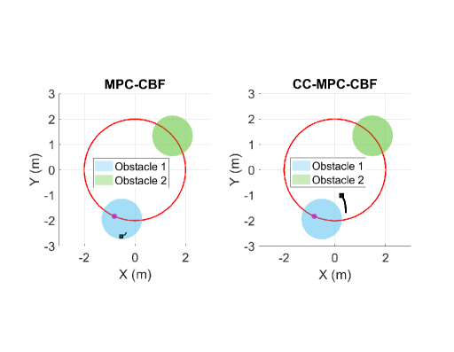
Figure 1: A snapshot of the tracking behaviors of the deterministic MPC-CBF and CC-MPC-CBF at time $k=90$ (top-down view): The red circle denotes the reference trajectory; the magenta solid point and black box maker represent the reference point and tracking point, respectively. Note that the black box is followed by a tail, which relates to the history tracking data.

V-C2 CC-MPC-CBF Settings

For the CC-MPC-CBF optimization problem formulated in Section III, we set the weighting matrices to be $\mathbf{P}=\mathbf{Q}=1000\mathbf{I}_{6\times 6}$ and $\mathbf{R}=\mathbf{I}_{3\times 3}$. The prediction horizon $N=15$. The CBF is defined by:

$$\begin{split}h(\mathbf{p}_{k},\mathbf{o}_{k})=\|\mathbf{p}_{k}-\mathbf{o}_{k}\|_{\mathbf{W}}^{2}-1.\end{split}$$ (24)

The weighting matrix $\mathbf{W}$ for obstacle 1 and obstacle 2 are set to be $\mathbf{W}_{\mathbf{o},1}=\mathrm{diag}([\frac{1}{r_{1}^{2}}\mathbf{I}_{1\times 3}])$ and $\mathbf{W}_{\mathbf{o},2}=\mathrm{diag}([\frac{1}{r_{2}^{2}}\mathbf{I}_{1\times 3}])$, respectively. The system is subject to state constraint $\mathbf{x}_{k}\in\mathcal{X}$ and input constraint $\mathbf{u}_{k}\in\mathcal{U}$,

$$\mathcal{X}=\left\{\mathbf{x}_{k}\in\mathbb{R}^{n}:\mathbf{x}_{\min}\leq\mathbf{x}_{k}\leq\mathbf{x}_{\max}\right\},$$ (25)

$$\mathcal{U}=\left\{\mathbf{u}_{k}\in\mathbb{R}^{m}:\mathbf{u}_{\min}\leq\mathbf{u}_{k}\leq\mathbf{u}_{\max}\right\}.$$

The lower and upper bounds are

$$\mathbf{x}_{\max},\mathbf{x}_{\min}=\pm 5\cdot\mathbf{I}_{6\times 1},\mathbf{u}_{\max},\mathbf{u}_{\min}=\pm 4\cdot\mathbf{I}_{3\times 1}.$$ (26)

Moreover, we define the collision avoidance probability threshold to be $\delta=0.03$ (thus confidence level $0.97$), which corresponds to $3\sigma$ confidence ellipsoid.

V-C3 Computer and Solver Settings

The simulated data is processed using Matlab 2019a on a 64-bit Intel core i7-9750H with a 2.6-GHz processor. Both the optimization problems formulated by CC-MPC-CBF, which is given by (18), and the standard MPC problems mentioned in Section IV, have been solved using a non-convex solver called IPOPT [24], which is implemented in the CaSadi framework that employs the YAMIP modeling language [25]. For the iterative convex optimization problem that is formulated in Section IV, we have used MOSEK, which is a convex solver.

V-D Performances of Different Approaches

V-D1 Tracking Performance of the deterministic MPC-CBF and CC-MPC-CBF

We compare the tracking performance of deterministic MPC-CBF and CC-MPC-CBF in a stochastic setting. Fig. 1 shows a snapshot of the tracking behavior at $k=90$. The actual trajectory (denoted by the black box) fails to avoid the moving obstacles when using deterministic MPC-CBF to track the desired trajectory $\mathbf{r}_{d}$. In contrast, CC-MPC-CBF successfully avoids collisions and achieves satisfying tracking performance. The successful collision avoidance rates with different levels of noise for both methods are provided in TABLE I. As shown in TABLE I, the performance of the deterministic MPC-CBF in ensuring successful MOCA is evaluated under different levels of noise, with $\sigma^{2}$ ranging from $0.0001$ to $0.5$ ($100$ trials conducted for each case). The results indicate that the deterministic MPC-CBF approach is not robust enough to guarantee successful MOCA in the presence of noise. As the noise level increases, the successful MOCA rate decreases. In contrast, the CC-MPC-CBF is robust to large sensing uncertainties as the successful collision avoidance rate remains $100\%$ even when $\sigma^{2}$ goes to $0.6$.

TABLE I: Successful collision avoidance rate for deterministic MPC-CBF and CC-MPC-CBF with different levels of noise.

Noise	$\sigma^{2}=0$	$\sigma^{2}=0.0001$	$\sigma^{2}=0.005$	$\sigma^{2}=0.01$	$\sigma^{2}=0.1$	$\sigma^{2}=0.3$	$\sigma^{2}=0.5$	$\sigma^{2}=0.6$
Deterministic MPC-CBF (%)	$100$	$91$	$53$	$38$	$17$	$12$	$8$	$7$
CC-MPC-CBF (%)	$100$	$100$	$100$	$100$	$100$	$100$	$100$	$100$

V-D2 Feasibility of CC-MPC-CBF with Different Parameters

To verify the observations presented in Remark 1, we conducted $100$ trials with varying levels of noise and set $\delta=0.97>\frac{1+\mathrm{erf}(0.5)}{2}$ to evaluate the feasibility of CC-MPC-CBF. The results are summarized in TABLE II, which clearly indicates that the feasibility of (18) decreases rapidly with an increase in $\sigma^{2}$. Furthermore, we recorded the instances of infeasibility, i.e., the time step $k$ at which it occurred, with different $\sigma^{2}$. The average value of $k$ across the 100 trials is provided in TABLE II, which reveals that this value decreases with increasing $\sigma^{2}$. This finding further supports the claim made in Proposition 1.

TABLE II: Feasibility performance of CC-MPC-CBF with different levels of noise $\sigma^{2}$.

Noise	$\sigma^{2}=0.7$	$\sigma^{2}=0.8$	$\sigma^{2}=0.9$	$\sigma^{2}=1$	$\sigma^{2}=2$	$\sigma^{2}=3$	$\sigma^{2}=4$	$\sigma^{2}=5$	$\sigma^{2}=6$
CC-MPC-CBF (%)	$100$	$100$	$100$	$93$	$60$	$35$	$10$	$2$	$0$
Infeasible at time $k$	\	\	\	$k=191$	$k=123$	$k=71$	$k=48$	$k=33$	$k=23$
Sequential Implementation (%)	$100$	$100$	$100$	$100$	$100$	$89$	$81$	$73$	$67$
Infeasible at time $k$	\	\	\	\	\	$k=182$	$k=167$	$k=144$	$k=122$

TABLE III: Feasibility performance of CC-MPC-CBF with hyperparameter $\gamma$.

Hyperparameter $\gamma$	$\gamma=1$	$\gamma=0.9$	$\gamma=0.8$	$\gamma=0.7$	$\gamma=0.6$	$\gamma=0.5$	$\gamma=0.4$	$\gamma=0.3$	$\gamma=0.2$	$\gamma=0.1$	$\gamma=0$
CC-MPC-CBF (%)	$100$	$100$	$100$	$100$	$100$	$93$	$87$	$61$	$42$	$25$	$13$
Infeasible at time $k$	\	\	\	\	\	$k=191$	$k=168$	$k=133$	$k=123$	$k=77$	$k=48$

The outcomes presented in TABLE III provide compelling support for the claim made in Remark 4. We initially set $\delta=0.97$ and $\sigma^{2}=1$. As indicated in TABLE II, some scenarios may be infeasible under the setting that $\gamma=0.5$. Next, we test the feasibility of CC-MPC-CBF with different $\gamma$. As shown in TABLE III, the results show that decreasing $\gamma$ leads to a higher rate of infeasibility.

As mentioned in Remark 5, increasing the prediction horizon $N$ may lead to infeasibility. To demonstrate this, we again set $\delta=0.97$, $\sigma^{2}=1$, and $\gamma=0.5$ and observe in TABLE IV that a larger $N$ results in more significant feasibility issues.

V-D3 Tracking Performance of the CC-MPC-DC and CC-MPC-CBF

In Fig.2, we compare the tracking performance of CC-MPC-DC [14] and the proposed CC-MPC-CBF (with different $N$ and $\gamma$). In accord with Remark 2, our results demonstrate that CC-MPC-CBF maintains the advantages of early obstacle avoidance when compared to CC-MPC-DC. Specifically, when we set $N=10$ and $\gamma=0.7$, CC-MPC-CBF starts avoiding obstacles at almost the same time as CC-MPC-DC with $N=15$. This means that we can achieve earlier obstacle avoidance without increasing the prediction horizon. Moreover, Fig.2 shows that an increase in $\gamma$ results in more conservative behavior.

V-D4 Feasibility Comparison: CC-MPC-CBF vs Sequential Implementation

By comparing the results shown in TABLE II, we can observe that the sequential implementation approach improves the feasibility of the CC-MPC-CBF formulation significantly, as stated in Remark 6. Due to the limitation of the paper length, we could not present and analyze the feasibility impact of $\gamma$ and $N$ on the sequential implementation approach. Nevertheless, it is worth noting that the conclusion aligns with that of CC-MPC-CBF.

V-D5 Computation efficiency of the sequential implementation approach

When the settings described in Section V-C are applied, it is important to note that the sequential approach proves to be more time-efficient compared to solving the CC-MPC-CBF optimization problem in a single run. In our simulation, after performing 100 trials, the average execution time of the sequential implementation amounts to $21.3\mathrm{s}$, which is considerably faster than the $38.8\mathrm{s}$ it takes to solve the CC-MPC-CBF optimization problem in one go.

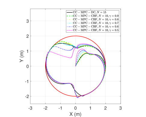
Figure 2: A comparison of the tracking performance of CC-MPC-DC and the proposed CC-MPC-CBF (with different $N$ and $\gamma$) (top-down view): The red circle denotes the reference trajectory; The curves with different line styles and colors indicate the tracking trajectories with different parameters.

TABLE IV: Feasibility performance of CC-MPC-CBF with different prediction horizons $N$.

Prediction horizons $N$	$N=5$	$N=10$	$N=15$	$N=20$	$N=30$	$N=50$	$N=60$
CC-MPC-CBF (%)	$100$	$100$	$93$	$88$	$60$	$0$	$0$
Infeasible at time $k$	\	\	$k=198$	$k=191$	$k=133$	$k=1$	$k=1$

VI Conclusion

In this paper, the MOCA problem in a stochastic scenario with unbounded uncertainties is addressed through the proposed CC-MPC-CBF approach, which combines MPC with chance-constrained CBFs to handle stochastic uncertainties and provides probabilistic guarantees on safety. A sequential implementation approach is also developed to improve the feasibility of the optimization of CC-MPC-CBF, which includes two sub-optimization problems, i.e., a standard MPC and a predictive safety filter. The effectiveness of the developed algorithms is demonstrated through numerous simulation results in a real-life MOCA example, which highlight their advantageous properties, such as robustness to large sensing uncertainties, high success rate for MOCA, fast computation speed, and feasibility for real-world applications. Overall, the proposed approach provides a promising solution to address the MOCA problem in stochastic systems with unbounded uncertainties.

References

[1]
R. M. Murray, Z. Li, and S. S. Sastry, A mathematical introduction to
robotic manipulation. CRC press,
2017.
[2]
X. Xu, J. W. Grizzle, P. Tabuada, and A. D. Ames, “Correctness guarantees for
the composition of lane keeping and adaptive cruise control,” IEEE
Transactions on Automation Science and Engineering, vol. 15, no. 3, pp.
1216–1229, 2017.
[3]
S. Zhao, D. V. Dimarogonas, Z. Sun, and D. Bauso, “A general approach to
coordination control of mobile agents with motion constraints,” IEEE
Transactions on Automatic Control, vol. 63, no. 5, pp. 1509–1516, 2017.
[4]
J. Alonso-Mora, T. Naegeli, R. Siegwart, and P. Beardsley, “Collision
avoidance for aerial vehicles in multi-agent scenarios,” Autonomous
Robots, vol. 39, pp. 101–121, 2015.
[5]
S. S. Mansouri, P. Karvelis, C. Kanellakis, D. Kominiak, and G. Nikolakopoulos,
“Vision-based MAV navigation in underground mine using convolutional
neural network,” in IECON 2019-45th Annual Conference of the IEEE
Industrial Electronics Society, vol. 1. IEEE, 2019, pp. 750–755.
[6]
H. Zhu and J. Alonso-Mora, “Chance-constrained collision avoidance for MAVs
in dynamic environments,” IEEE Robotics and Automation Letters,
vol. 4, no. 2, pp. 776–783, 2019.
[7]
B. Lindqvist, S. S. Mansouri, A.-a. Agha-mohammadi, and G. Nikolakopoulos,
“Nonlinear MPC for collision avoidance and control of UAVs with dynamic
obstacles,” IEEE Robotics and Automation Letters, vol. 5, no. 4, pp.
6001–6008, 2020.
[8]
J. Zeng, B. Zhang, and K. Sreenath, “Safety-critical model predictive control
with discrete-time control barrier function,” in 2021 American Control
Conference (ACC). IEEE, 2021, pp.
3882–3889.
[9]
Y. Emam, P. Glotfelter, and M. Egerstedt, “Robust barrier functions for a
fully autonomous, remotely accessible swarm-robotics testbed,” in 2019
IEEE 58th Conference on Decision and Control (CDC). IEEE, 2019, pp. 3984–3990.
[10]
M. Jankovic, “Robust control barrier functions for constrained stabilization
of nonlinear systems,” Automatica, vol. 96, pp. 359–367, 2018.
[11]
S. Kolathaya and A. D. Ames, “Input-to-state safety with control barrier
functions,” IEEE Control Systems Letters, vol. 3, no. 1, pp.
108–113, 2018.
[12]
M. Ohnishi, L. Wang, G. Notomista, and M. Egerstedt, “Barrier-certified
adaptive reinforcement learning with applications to brushbot navigation,”
IEEE Transactions on Robotics, vol. 35, no. 5, pp. 1186–1205, 2019.
[13]
A. J. Taylor and A. D. Ames, “Adaptive safety with control barrier
functions,” in 2020 American Control Conference (ACC). IEEE, 2020, pp. 1399–1405.
[14]
H. Zhu and J. Alonso-Mora, “Chance-constrained collision avoidance for MAVs
in dynamic environments,” IEEE Robotics and Automation Letters,
vol. 4, no. 2, pp. 776–783, 2019.
[15]
A. Clark, “Control barrier functions for stochastic systems,”
Automatica, vol. 130, p. 109688, 2021.
[16]
A. Agrawal and K. Sreenath, “Discrete control barrier functions for
safety-critical control of discrete systems with application to bipedal robot
navigation.” in Robotics: Science and Systems, vol. 13. Cambridge, MA, USA, 2017.
[17]
G. Grimmett and D. Stirzaker, Probability and Random Processes. Oxford university press, 2020.
[18]
A. C. Rencher and G. B. Schaalje, Linear Models in Statistics. John Wiley & Sons, 2008.
[19]
L. Blackmore, M. Ono, and B. C. Williams, “Chance-constrained optimal path
planning with obstacles,” IEEE Transactions on Robotics, vol. 27,
no. 6, pp. 1080–1094, 2011.
[20]
J. Zeng, Z. Li, and K. Sreenath, “Enhancing feasibility and safety of
nonlinear model predictive control with discrete-time control barrier
functions,” in 2021 60th IEEE Conference on Decision and Control
(CDC). IEEE, 2021, pp. 6137–6144.
[21]
M. Morari and J. H. Lee, “Model predictive control: past, present and
future,” Computers & Chemical Engineering, vol. 23, no. 4-5, pp.
667–682, 1999.
[22]
M. L. Darby and M. Nikolaou, “MPC: Current practice and challenges,”
Control Engineering Practice, vol. 20, no. 4, pp. 328–342, 2012.
[23]
A. D. Ames, S. Coogan, M. Egerstedt, G. Notomista, K. Sreenath, and P. Tabuada,
“Control barrier functions: Theory and applications,” in 2019 18th
European control conference (ECC). IEEE, 2019, pp. 3420–3431.
[24]
L. T. Biegler and V. M. Zavala, “Large-scale nonlinear programming using
ipopt: An integrating framework for enterprise-wide dynamic optimization,”
Computers & Chemical Engineering, vol. 33, no. 3, pp. 575–582, 2009.
[25]
J. Lofberg, “YALMIP: A toolbox for modeling and optimization in MATLAB,”
in 2004 IEEE International Conference on Robotics and Automation
(ICRA). IEEE, 2004, pp. 284–289.