Rational Solutions of the Fifth Painlevé Equation.
Generalised Laguerre Polynomials

Abstract

In this paper rational solutions of the fifth Painlevé equation are discussed. There are two classes of rational solutions of the fifth Painlevé equation, one expressed in terms of the generalised Laguerre polynomials, which are the main subject of this paper, and the other in terms of the generalised Umemura polynomials. Both the generalised Laguerre polynomials and the generalised Umemura polynomials can be expressed as Wronskians of Laguerre polynomials specified in terms of specific families of partitions. The properties of the generalised Laguerre polynomials are determined and various differential-difference and discrete equations found. The rational solutions of the fifth Painlevé equation, the associated $\sigma$-equation and the symmetric fifth Painlevé system are expressed in terms of generalised Laguerre polynomials. Non-uniqueness of the solutions in special cases is established and some applications are considered. In the second part of the paper, the structure of the roots of the polynomials are investigated for all values of the parameter. Interesting transitions between root structures through coalescences at the origin are discovered, with the allowed behaviours controlled by hook data associated with the partition. The discriminants of the generalised Laguerre polynomials are found and also shown to be expressible in terms of partition data. Explicit expressions for the coefficients of a general Wronskian Laguerre polynomial defined in terms of a single partition are given.

• Keywords: Painlevé equation, rational solutions, Laguerre polynomials, discriminant, partition, Wronskian.

Dedicated to Athanassios S. Fokas on the occasion of his 70th anniversary for his many contributions to studies of integrable nonlinear differential equations, including Painlevé equations.

1 Introduction

The fifth Painlevé equation is given by

$$\frac{{\rm d}^{2}{w}}{{{\rm d}{z}}^{2}}=\left(\frac{1}{2w}+\frac{1}{w-1}\right)\left(\frac{{\rm d}{w}}{{{\rm d}{z}}}\right)^{\!\!2}-\frac{1}{z}\frac{{\rm d}{w}}{{{\rm d}{z}}}+\frac{(w-1)^{2}(\alpha w^{2}+{\beta})}{z^{2}w}+\frac{\gamma w}{z}+\frac{\delta w(w+1)}{w-1},$$ (1.1)

with $\alpha$, $\beta$, $\gamma$ and $\delta$ constants. In the generic case of (1.1) when $\delta\not=0$, then we set $\delta=-\tfrac{1}{2}$, without loss of generality (by rescaling $z$ if necessary) and obtain

$$\frac{{\rm d}^{2}{w}}{{{\rm d}{z}}^{2}}=\left(\frac{1}{2w}+\frac{1}{w-1}\right)\left(\frac{{\rm d}{w}}{{{\rm d}{z}}}\right)^{\!\!2}-\frac{1}{z}\frac{{\rm d}{w}}{{{\rm d}{z}}}+\frac{(w-1)^{2}(\alpha w^{2}+{\beta})}{z^{2}w}+\frac{\gamma w}{z}-\frac{w(w+1)}{2(w-1)},$$ (1.2)

which we will refer to as P_V.

The six Painlevé equations (P_I–P_VI), were discovered by Painlevé, Gambier and their colleagues whilst studying second order ordinary differential equations of the form

$$\frac{{\rm d}^{2}{w}}{{{\rm d}{z}}^{2}}=F\left(z,w,\frac{{\rm d}{w}}{{{\rm d}{z}}}\right),$$ (1.3)

where $F$ is rational in ${\rm d}w/{\rm d}z$ and $w$ and analytic in $z$. The Painlevé transcendents, i.e. the solutions of the Painlevé equations, can be thought of as nonlinear analogues of the classical special functions. Iwasaki, Kimura, Shimomura and Yoshida [34] characterize the six Painlevé equations as “the most important nonlinear ordinary differential equations” and state that “many specialists believe that during the twenty-first century the Painlevé functions will become new members of the community of special functions”. Subsequently the Painlevé transcendents are a chapter in the NIST Digital Library of Mathematical Functions [62, §32].

The general solutions of the Painlevé equations are transcendental in the sense that they cannot be expressed in terms of known elementary functions and so require the introduction of a new transcendental function to describe their solution. However, it is well known that all the Painlevé equations, except P_I, possess rational solutions, algebraic solutions and solutions expressed in terms of the classical special functions — Airy, Bessel, parabolic cylinder, Kummer and hypergeometric functions, respectively — for special values of the parameters, see, e.g. [14, 23, 29] and the references therein. These hierarchies are usually generated from “seed solutions” using the associated Bäcklund transformations and frequently can be expressed in the form of determinants.

Vorob’ev [72] and Yablonskii [76] expressed the rational solutions of P_II in terms of special polynomials, now known as the Yablonskii–Vorob’ev polynomials, which were defined through a second-order, bilinear differential-difference equation. Subsequently Kajiwara and Ohta [37] derived a determinantal representation of the polynomials, see also [35, 36]. Okamoto [57] obtained special polynomials, analogous to the Yablonskii–Vorob’ev polynomials, which are associated with some of the rational solutions of P_IV. Noumi and Yamada [54] generalized Okamoto’s results and expressed all rational solutions of P_IV in terms of special polynomials, now known as the generalized Hermite polynomials $H_{m,n}(z)$ and generalized Okamoto polynomials $Q_{m,n}(z)$, both of which are determinants of sequences of Hermite polynomials; see also [38].

Umemura [69] derived special polynomials associated with certain rational and algebraic solutions of P_III and P_V, which are determinants of sequences of associated Laguerre polynomials. (The original manuscript was written by Umemura in 1996 for the proceedings of the conference “Theory of nonlinear special functions: the Painlevé transcendents” in Montreal, which were not published; see [61].) Subsequently there have been further studies of rational and algebraic solutions of P_V [13, 17, 41, 47, 52, 58, 73]. Several of these papers are concerned with the combinatorial structure and determinant representation of the generalised Laguerre polynomials, often related to the Hamiltonian structure and affine Weyl symmetries of the Painlevé equations. Additionally the coefficients of these special polynomials have some interesting combinatorial properties [67, 68, 69]. See also [50] and results on the combinatorics of the coefficients of Wronskian Hermite polynomials [8] and Wronskian Appell polynomials [7].

We define generalised Laguerre polynomials as Wronskians of a sequence of associated Laguerre polynomials specified in terms of a partition of an integer. We give a short introduction to the combinatorial concepts in §2 and record several equivalent definitions of a generalised Laguerre polynomial in §3, where we also show that the polynomials satisfy various differential-difference equations and discrete equations. In §4 we express a family of rational solution of P_V (1.2) in terms of the generalised Laguerre polynomials. For certain values of the parameter, we show that the solutions are not unique. Rational solutions of the P_V $\sigma$-equation, the second-order, second-degree differential equation associated with the Hamiltonian representation of P_V, are considered in §5, which includes a discussion of some applications. In §6 we describe rational solutions of the symmetric P_V system. Properties of generalised Laguerre polynomials are established in §7 as well as an explicit description of all partitions with $2$-core of size $k$ and $2$-quotient $(\boldsymbol{\lambda},\boldsymbol{\emptyset})$ for all partitions $\boldsymbol{\lambda}$. Then in §8 we obtain the discriminants of the polynomials, describe the patterns of roots as a function of the parameter and explain how the roots move as the parameter varies. Finally, we show that many of the results in the last section can be expressed in terms of combinatorial properties of the underlying partition. We also obtain explicit expressions for the coefficients of Wronskian Laguerre polynomials that depend on a single partition using the hooks of the partition.

2 Partitions

Partitions will appear throughout this article. We give a brief description of the key ideas. Useful references include [44, 64]. A partition $\boldsymbol{\lambda}=(\lambda_{1},\lambda_{2},\ldots,\lambda_{r})$ is a sequence of non-increasing integers $\lambda_{1}\geq\lambda_{2}\geq\ldots\geq\lambda_{r}$. We sometimes set $r=\ell(\boldsymbol{\lambda})$. The partition $\boldsymbol{\emptyset}$ represents the unique partition of zero. We define $|\boldsymbol{\lambda}|=\lambda_{1}+\lambda_{2}+\dots+\lambda_{r}$. The associated degree vector $\boldsymbol{h}_{\boldsymbol{\lambda}}=(h_{1},h_{2},\ldots,h_{r})$ is a sequence of distinct integers $h_{1}>h_{2}>\ldots>h_{r}>0$ related to partition elements via

$$\lambda_{j}=h_{j}-r+j,\qquad j=1,2,\ldots,r.$$ (2.1)

We often write $\boldsymbol{h}$ rather than $\boldsymbol{h}_{\boldsymbol{\lambda}}$. Define the Vandermonde determinant $\Delta(\boldsymbol{h})$ as

$$\Delta(\boldsymbol{h})=\prod_{1\leq j<k\leq r}(h_{k}-h_{j}).$$ (2.2)

Partitions are usefully represented as Young diagrams by stacking $r$ rows of boxes of decreasing length $\lambda_{j}$ for $j=1,2,\dots,r$ on top of each other. Reflecting a Young diagram in the main diagonal gives the diagram corresponding to the conjugate partition $\boldsymbol{\lambda}^{*}$. Young’s lattice is the lattice of all partitions partially ordered by inclusion of the corresponding Young diagrams. That is, $\widetilde{\boldsymbol{\lambda}}\leq\boldsymbol{\lambda}$ if $\widetilde{\lambda}_{i}\leq\lambda_{i}$ for $i=1,2,\dots,\ell(\widetilde{\boldsymbol{\lambda}})$. We write $\widetilde{\boldsymbol{\lambda}}<_{j}\boldsymbol{\lambda}$ if $|\widetilde{\boldsymbol{\lambda}}|+j=|\boldsymbol{\lambda}|.$ Let $F_{\boldsymbol{\lambda}}$ denote the number of paths in the Young lattice from $\boldsymbol{\lambda}$ to $\boldsymbol{\emptyset}$, and $F_{\boldsymbol{\lambda}/\widetilde{\boldsymbol{\lambda}}}$ the number of paths from $\boldsymbol{\lambda}$ to $\widetilde{\boldsymbol{\lambda}}$. Explicitly

$$F_{\boldsymbol{\lambda}/\widetilde{\boldsymbol{\lambda}}}=(|\boldsymbol{\lambda}|-|\widetilde{\boldsymbol{\lambda}}|)!\text{ det}\,\left[\frac{1}{(\lambda_{j}-\widetilde{\lambda}_{k}-j+k)!}\right]_{j,k=1}^{\ell(\boldsymbol{\lambda})}.$$

A hook length $h_{jk}$ is assigned to box $(j,k)$ in the Young diagram via

$$h_{j,k}=\lambda_{j}+{\lambda}^{*}_{k}-j-k+1.$$ (2.3)

The hook length counts the number of boxes to the right of and below box $(j,k)$ plus one. Thus

$$F_{\boldsymbol{\lambda}}=\frac{|\boldsymbol{\lambda}|!}{\prod_{h\in\mathcal{H}_{\boldsymbol{\lambda}}}h},$$

where $\mathcal{H}_{\boldsymbol{\lambda}}$ is the set of all hook lengths. The entries of the degree vector $\boldsymbol{h}_{\boldsymbol{\lambda}}$ are the hooks in the first column of the Young diagram. Examples of Young diagrams and the corresponding hook lengths are given in Figure 2.1.

A partition can be represented as $p+1$ smaller partitions known as the $p$-core $\overline{\boldsymbol{\lambda}}$ and $p$-quotient $(\boldsymbol{\nu}_{1},\dots,\boldsymbol{\nu}_{p})$. A partition is a $p$-core partition if it contains no hook lengths of size $p$. Therefore the example partition $(2,1)$ is a $2$-core and $\boldsymbol{\lambda}=(4^{2},2,1^{3})$ is both a $6$- and $7$-core. We only consider $p=2$ here. The hooks of size $2$ are vertical or horizontal dominoes. We note that all $2$-cores are staircase partitions $\overline{\boldsymbol{\lambda}}=(k,k-1,\ldots,1)$.

The $2$-core of a partition is found by sequentially removing all hooks of size $2$ from the Young diagram such that at each step the diagram represents a partition. The terminating Young diagram defines the $2$-core, which we denote $\overline{\boldsymbol{\lambda}}$. It does not depend on the order in which the hooks are removed. For example, the partition $(4^{2},2,1^{3})$ has $2$-core $\overline{\boldsymbol{\lambda}}=(2,1)$. Figure 2.1(a) shows that there are three choices of domino that may be removed at the first step. The $2$-height $\text{ht}(\boldsymbol{\lambda})$ (or $2$-sign) of partition $\boldsymbol{\lambda}$ is the (unique) number of vertical dominoes removed from $\boldsymbol{\lambda}$ to obtain its $2$-core. Equivalently, the $2$-height is the number of vertical dominoes in any domino tiling of the Young diagram of $\boldsymbol{\lambda}$.

The $2$-quotient records how the dominoes are removed from a partition to obtain its core. James’ $p$-abacus [31] is a useful tool to determine the quotient, and provides an alternative visual representation of a partition. A $2$-abacus consists of left and right vertical runners with bead positions labelled $0,2,4,\ldots$ (left) and $1,3,5,\ldots$ (right) from top to bottom. To represent a partition on the $2$-abacus, place a bead at the points corresponding to each element of the degree vector $\boldsymbol{h}$. Since a partition can have as many $0$’s as we like, we allow an abacus to have any number of initial beads and any number of empty beads after the last bead. There are, therefore, an infinite set of abaci associated to each partition, according to the location of the first unoccupied slot. We return to this point below. The parts of a partition are read from its abacus by counting the number of empty spaces before each bead.

A bead with no bead directly above it on the same runner corresponds to a hook of length $2$ in the Young diagram. The $2$-core $\overline{\boldsymbol{\lambda}}$ is found from the abacus by sliding all beads vertically up as far as possible and reading off the resulting partition. Figure 2.1 shows the Young diagram and hooklengths of $(4^{2},2,1^{3})$ in (a), an abacus representation in (c), its $2$-core $\overline{\boldsymbol{\lambda}}=(2,1)$ in (b) and the abacus corresponding to $\overline{\boldsymbol{\lambda}}$ that is obtained from (c) by pushing up all beads.

(a) ${\boldsymbol{\lambda}}$

(b) $\overline{\boldsymbol{\lambda}}$

(c) ${\boldsymbol{\lambda}}$

(d) $\overline{\boldsymbol{\lambda}}$

Figure 2.1: The Young diagrams including hook length corresponding to (a) $\boldsymbol{\lambda}=(4^{2},2,1^{3})$ and its core (b) $\overline{\boldsymbol{\lambda}}=(2,1)$, and corresponding abacus diagrams (c) and (d).

The $2$-quotient is an ordered pair of partitions $(\boldsymbol{\nu}_{1},\boldsymbol{\nu}_{2})$ that encodes how many places the beads on each runner are moved to obtain the $2$-core. The $2$-quotient ordering is specified by ensuring the $2$-core has at least as many beads on the second runner as the first. One can always add a bead to the left runner of the partition abacus and shift all subsequent beads one place if this condition is not met [74], swapping the order of the quotient partitions. Consequently, the relationship between a partition and its $2$-core of size $k$ and $2$-quotient $(\boldsymbol{\nu}_{1},\boldsymbol{\nu}_{2})$ is bijective. In the running example, one bead on the left runner is moved one place and another bead is moved three places. This is recorded in the partition $\boldsymbol{\nu}_{1}=(3,1)$. Only one bead is moved on runner 2, by one space, and so $\boldsymbol{\nu}_{2}=(1)$. Therefore the $2$-core and $2$-quotient of ${\boldsymbol{\lambda}}=(4^{2},2,1^{3})$ are $(2,1)$ and $((3,1),(1))$ respectively.

While we do not know of an explicit representation of the core and quotient for a generic partition, nor vice versa, the corresponding partitions can easily be found case by case and the bijection is known in some special families of partitions. Partitions with $2$-core $k$ and $2$-quotient $(\boldsymbol{\nu},\boldsymbol{\emptyset})$ will be important in this article. For such partitions, we now determine the (unordered) first column hooks of the corresponding partition $\boldsymbol{\Lambda}(k,\boldsymbol{\nu})$. Find the degree vector $\boldsymbol{h}_{\boldsymbol{\nu}}$ and place beads on the $2$-abacus in positions

$$\left\{2h_{i}\right\}_{i=1}^{r}\cup\{2j-1\}_{j=1}^{r+k}.$$ (2.4)

We read off the corresponding partition $\boldsymbol{\Lambda}(k,\boldsymbol{\nu})$ from the position of the beads on the abacus. The first column hooks given by (2.4) must be ordered before using (2.1) to obtain the partition, which is why we cannot give an expression for $\boldsymbol{\Lambda}(k,\boldsymbol{\nu})$ for generic partitions $\boldsymbol{\nu}$. As an example take $k=3$ and $\boldsymbol{\nu}=(4,2,1)$. Then $\boldsymbol{h}_{\boldsymbol{\nu}}=(6,3,1)$. It follows from (2.4) that the abacus of the partition $\boldsymbol{\Lambda}(3,(4,2,1))$ has beads in places $2,6,12$ and $1,3,5,7,9,11$. Therefore $\boldsymbol{h}_{\boldsymbol{\Lambda}}=(12,11,9,7,6,5,3,2,1)$ and thus $\boldsymbol{\Lambda}(3,(4,2,1))=(4^{2},3,2^{3},1^{3})$. In section 7, we use the first column hook set (2.4) to determine an explicit formula for the family of partitions with $2$-core $k$ and $2$-quotient $(((m+1)^{n}),\boldsymbol{\emptyset})$.

3 Generalised Laguerre polynomials

Definition 3.1.

The generalised Laguerre polynomial $T_{m,n}^{(\mu)}(z)$, which is a polynomial of degree $(m+1)n$, is defined by

$$T_{m,n}^{(\mu)}(z)=\det\left[\frac{{\rm d}^{j+k}}{{\rm d}z^{j+k}}L_{m+n}^{(\mu+1)}(z)\right]_{j,k=0}^{n-1},\qquad m\geq 0,\quad n\geq 1,$$ (3.1)

where $L_{n}^{(\alpha)}(z)$ is the associated Laguerre polynomial

$$L_{n}^{(\alpha)}(z)=\frac{z^{-\alpha}\,{\rm e}^{z}}{n!}\frac{{\rm d}^{n}{}}{{{\rm d}{z}}^{n}}\left(z^{n+\alpha}\,{\rm e}^{-z}\right),\qquad n\geq 0.$$ (3.2)

Lemma 3.2.

The generalised Laguerre polynomial $T_{m,n}^{(\mu)}(z)$ can also be written as the Wronskian

$$T_{m,n}^{(\mu)}(z) =(-1)^{n(n-1)/2}\operatorname{Wr}\left(L_{m+n}^{(n+\mu)}(z),L_{m+n-1}^{(n+\mu)}(z),\ldots,L_{m+1}^{(n+\mu)}(z)\right)$$

$$=\operatorname{Wr}\left(L_{m+1}^{(n+\mu)}(z),L_{m+2}^{(n+\mu)}(z),\ldots,L_{m+n}^{(n+\mu)}(z)\right).$$ (3.3)

Proof.

We use

$$\frac{{\rm d}^{k}}{{\rm d}z^{k}}L_{n}^{(\alpha)}(z)=\begin{cases}(-1)^{k}L_{n-k}^{(\alpha+k)}(z),\quad&k\leq n,\\ 0,&\text{otherwise},\end{cases}$$ (3.4)

cf. [62, equation (18.9.23)], to write the determinant form of $T_{m,n}^{(\mu)}(z)$ as a Wronskian

$$\det\left[\frac{{\rm d}^{j+k}}{{\rm d}z^{j+k}}L_{m+n}^{(\mu+1)}(z)\right]_{j,k=0}^{n-1}=(-1)^{n(n-1)/2}\operatorname{Wr}\left(L_{m+n}^{(\mu+1)}(z),L_{m+n-1}^{(\mu+2)}(z),\ldots,L_{m+1}^{(\mu+n)}(z)\right).$$

Using the result

$$L_{m}^{(\alpha)}(z)=L_{m}^{(\alpha+1)}(z)-L_{m-1}^{(\alpha+1)}(z),$$ (3.5)

[62, equation (18.9.13)], it can be shown using induction that

$$L_{m+k}^{(\alpha+1-k)}(z)=L_{m+k}^{(\alpha)}(z)+\sum_{j=1}^{k-1}(-1)^{k-j}\binom{k-1}{j-1}L_{m+j}^{(\alpha)}(z).$$

Hence setting $\alpha=\mu+n$ gives

$$L_{m+k}^{(\mu+n+1-k)}(z)=L_{m+k}^{(\mu+n)}(z)+\sum_{j=1}^{k-1}(-1)^{k-j}\binom{k-1}{j-1}L_{m+j}^{(\mu+n)}(z),\qquad k=1,2,\ldots,n,$$ (3.6)

and so we obtain

$$T_{m,n}^{(\mu)}(z) =(-1)^{n(n-1)/2}$$

$$\times\operatorname{Wr}\left({L_{m+n}^{(n+\mu)}(z)+\sum_{j=1}^{n}(-1)^{n-j}\binom{n-1}{j-1}L_{m+j}^{(n+\mu)},\ldots,L_{m+2}^{(n+\mu)}(z)-L_{m+1}^{(n+\mu)}(z),L_{m+1}^{(n+\mu)}(z)}\right).$$

Since we can add a multiple of any column to any other column without changing the Wronskian determinant, we keep the last term in each sum:

$$T_{m,n}^{(\mu)}(z)=(-1)^{n(n-1)/2}\operatorname{Wr}\left(L_{m+n}^{(n+\mu)}(z),L_{m+n-1}^{(n+\mu)}(z),\ldots,L_{m+1}^{(n+\mu)}(z)\right).$$ (3.7)

On interchanging the $j^{\rm th}$ column with the $(n-j+1)^{\rm th}$ column, we find

$$T_{m,n}^{(\mu)}(z)=\operatorname{Wr}\left(L_{m+1}^{(n+\mu)}(z),L_{m+2}^{(n+\mu)}(z),\ldots,L_{m+n}^{(n+\mu)}(z)\right).$$ (3.8)

∎

We remark that

$$T_{0,m-1}^{(n-m+1)}(z)=\operatorname{Wr}\left(L_{1}^{(n)}(z),L_{2}^{(n)}(z),\ldots,L_{m-1}^{(n)}(z)\right)=(-1)^{\lfloor m/2\rfloor}L_{m-1}^{(-m-n)}(-z).$$

Definition 3.3.

Bonneux and Kuiljaars [9], see also [21, 22, 26], define a Wronskian of Laguerre polynomials

$$\Omega_{\boldsymbol{\lambda}}^{(\alpha)}(z)=\operatorname{Wr}\left(L_{h_{1}}^{(\alpha)}(z),L_{h_{2}}^{(\alpha)}(z),\ldots,L_{h_{r}}^{(\alpha)}(z)\right),$$ (3.9)

in terms of the degree vector $\boldsymbol{h}=(h_{1},h_{2},\ldots,h_{r})$ of partition $\boldsymbol{\lambda}=(\lambda_{1},\lambda_{2},\ldots,\lambda_{r})$. Hence

$$T_{m,n}^{(\mu)}(z)=(-1)^{n(n-1)/2}\,\Omega_{\boldsymbol{\lambda}}^{(n+\mu)}(z),$$ (3.10)

where the partition is $\boldsymbol{\lambda}=((m+1)^{n})$.

Definition 3.4.

The elementary Schur polynomials $p_{j}(\boldsymbol{t})$, for $j\in\mathbb{Z}$, in terms of the variables $\boldsymbol{t}=(t_{1},t_{2},\ldots)$, are defined by the generating function

$$\sum_{j=0}^{\infty}p_{j}(\boldsymbol{t})\,x^{j}=\exp\left(\sum_{j=1}^{\infty}t_{j}\,x^{j}\right),\qquad p_{j}(\boldsymbol{t})=0,\quad\text{for}\quad j<0,$$ (3.11)

with $p_{0}(\boldsymbol{t})=1$. The Schur polynomial $S_{\boldsymbol{\lambda}}(\boldsymbol{t})$ for the partition $\boldsymbol{\lambda}$ is given by

$$S_{\boldsymbol{\lambda}}(\boldsymbol{t})={\rm det}\begin{bmatrix}p_{\lambda_{j}+k-j}(\boldsymbol{t})\end{bmatrix}_{j,k=1}^{r}.$$ (3.12)

The generalised Laguerre polynomial $T_{m,n}^{(\mu)}(z)$ can be expressed as a Schur polynomial, as shown in the following Lemma.

Lemma 3.5.

The generalised Laguerre polynomial $T_{m,n}^{(\mu)}(z)$ is the Schur polynomial

$$T_{m,n}^{(\mu)}(z)=(-1)^{n(n-1)/2}S_{\boldsymbol{\lambda}}(\boldsymbol{t}),$$ (3.13)

where $\boldsymbol{\lambda}=((m+1)^{n})$ and

$$t_{j}=\frac{\mu+n+1}{j}-z,\qquad j=1,2,\ldots\ .$$ (3.14)

Proof.

Since

$$\frac{\partial^{j}p_{m}}{\partial t_{1}^{j}}=p_{m-j},$$

the Schur polynomial (3.12) can be written as the Wronskian

$$S_{\boldsymbol{\lambda}}(\boldsymbol{t})=\operatorname{Wr}\left(p_{\lambda_{n}},{p_{\lambda_{n-1}+1}},\ldots,p_{\lambda_{1}+n-1}\right),$$ (3.15)

for any partition $\boldsymbol{\lambda}$, where the Wronskian is evaluated with respect to $t_{1}$. The choice of $t_{j}$ defined in (3.13) leads to

$$p_{j}(\boldsymbol{t})=L_{j}^{(\mu+n)}(-z),\qquad j=0,1,\ldots\ .$$ (3.16)

Set $\boldsymbol{\lambda}=((m+1)^{n})$, then (3.13) follows from (3.15) by re-ordering rows and columns and letting $z\to-z$. ∎

Definition 3.6.

Define the polynomial $\widehat{T}_{m,n}^{(\mu)}(z)$

$$\widehat{T}_{m,n}^{(\mu)}(z)=\det\left[\frac{{\rm d}^{j+k}}{{\rm d}z^{j+k}}L_{m+n}^{(\mu+1)}(-z)\right]_{j,k=0}^{n-1},\quad m\geq 0,\quad n\geq 1,$$ (3.17)

with $L_{n}^{(\alpha)}(z)$ the associated Laguerre polynomial.

Remark 3.7.

We note that

$$T_{m,n}^{(\mu)}(-z)=\widehat{T}_{m,n}^{(\mu)}(z).$$ (3.18)

Lemma 3.8.

The generalised Laguerre polynomial $T_{m,n}^{(\mu)}(z)$ has the discrete symmetry

$$T_{m,n}^{(\mu)}(z)=(-1)^{\lfloor(m+n+1)/2\rfloor}\,T_{n-1,m+1}^{(-\mu-2n-2m-2)}(-z).$$ (3.19)

Proof.

Apply the standard relation

$$S_{\boldsymbol{\lambda}}(\boldsymbol{t})=S_{\boldsymbol{\lambda}^{*}}(-\boldsymbol{t}).$$ (3.20)

with $\boldsymbol{\lambda}^{*}=(n^{m+1})$ to the Schur form of the generalised Laguerre polynomial (3.5). ∎

Lemma 3.9.

The generalised Laguerre polynomial $T_{m,n}^{(\mu)}(z)$ can also be written as the determinants

$$T_{m,n}^{(\mu)}(z) =\det\left[L_{m+n}^{(\mu+j+k+1)}(z)\right]_{j,k=0}^{n-1}, m\geq 0,\quad n\geq 1,$$ (3.21a)

$$T_{m,n}^{(\mu)}(z) =\det\left[L_{m+n-j-k}^{(\mu+2n-1)}(z)\right]_{j,k=0}^{n-1}, m\geq 0,\quad n\geq 1,$$ (3.21b)

$$T_{m,n}^{(\mu)}(z) =\det\left[L_{m+2-n+j+k}^{(\mu+2n-1)}(z)\right]_{j,k=0}^{n-1}, m\geq 0,\quad n\geq 1,$$ (3.21c)

$$T_{m,n}^{(\mu)}(z) =(-1)^{\lfloor n/2\rfloor}\det\left[L_{m+j+1}^{(\mu+n+k)}(z)\right]_{j,k=0}^{n-1}, m\geq 0,\quad n\geq 1,$$ (3.21d)

$$T_{m,n}^{(\mu)}(z) =(-1)^{\lfloor n/2\rfloor}\det\left[L_{m+1+j-k}^{(\mu+2n-1)}(z)\right]_{j,k=0}^{n-1}, m\geq 0,\quad n\geq 1,$$ (3.21e)

where $L_{n}^{(\alpha)}(z)$ is the Laguerre polynomial with $L_{n}^{(\alpha)}(z)=0$ if $n<0$.

Proof.

These identities are easily proved using the well-known formulae (3.4) and (3.5), and properties of Wronskians in either (3.1) or (3.3).

∎

Lemma 3.10.

The generalised Laguerre polynomial $T_{m,n}^{(\mu)}(z)$ satisfies the second-order, differential-difference equation

$$T_{m,n}^{(\mu)}\frac{{\rm d}^{2}{T_{m,n}^{(\mu)}}}{{{\rm d}{z}}^{2}}-\left(\frac{{\rm d}{T_{m,n}^{(\mu)}}}{{{\rm d}{z}}}\right)^{\!2}=T_{m+1,n-1}^{(\mu)}T_{m-1,n+1}^{(\mu)}.$$ (3.22)

Proof.

According to Sylvester [65], see also [48], if $\mathcal{A}_{n}(\varphi)$ is the double Wronskian given by

$$\mathcal{A}_{n}(\varphi)=\det\left[\frac{{\rm d}^{j+k}{\varphi}}{{{\rm d}{z}}^{j+k}}\right]_{j,k=0}^{n-1}=\operatorname{Wr}\left(\varphi,\frac{{\rm d}{\varphi}}{{{\rm d}{z}}},\ldots,\frac{{\rm d}^{n-1}{\varphi}}{{{\rm d}{z}}^{n-1}}\right),$$

then $\mathcal{A}_{n}(\varphi)$ satisfies the

$$\mathcal{A}_{n}\frac{{\rm d}^{2}{\mathcal{A}_{n}}}{{{\rm d}{z}}^{2}}-\left(\frac{{\rm d}{\mathcal{A}_{n}}}{{{\rm d}{z}}}\right)^{\!2}=\mathcal{A}_{n+1}\mathcal{A}_{n-1},$$ (3.23)

which is now known as the Toda equation. From (3.1)

$$T_{m,n}^{(\mu)}=\det\left[\frac{{\rm d}^{j+k}{L_{m+n}^{(\mu)}}}{{{\rm d}{z}}^{j+k}}\right]_{j,k=0}^{n-1}=\operatorname{Wr}\left(L_{m+n}^{(\mu)},\frac{{\rm d}{L_{m+n}^{(\mu)}}}{{{\rm d}{z}}},\ldots,\frac{{\rm d}^{n-1}{L_{m+n}^{(\mu)}}}{{{\rm d}{z}}^{n-1}}\right).$$

If we let $\varphi=L_{m+n}^{(\mu)}$ and $\mathcal{A}_{n}\left(L_{m+n}^{(\mu)}\right)=T_{m,n}^{(\mu)}$, then we need to show that

$$\mathcal{A}_{n+1}\left(L_{m+n}^{(\mu)}\right)=T_{m-1,n+1}^{(\mu)},\qquad\mathcal{A}_{n-1}\left(L_{m+n}^{(\mu)}\right)=T_{m+1,n-1}^{(\mu)}.$$

By definition

$$\mathcal{A}_{n+1}\left(L_{m+n}^{(\mu)}\right) =\operatorname{Wr}\left(L_{m+n}^{(\mu)},\frac{{\rm d}{L_{m+n}^{(\mu)}}}{{{\rm d}{z}}},\ldots,\frac{{\rm d}^{n}{L_{m+n}^{(\mu)}}}{{{\rm d}{z}}^{n}}\right)=T_{m-1,n+1}^{(\mu)},$$

$$\mathcal{A}_{n-1}\left(L_{m+n}^{(\mu)}\right) =\operatorname{Wr}\left(L_{m+n}^{(\mu)},\frac{{\rm d}{L_{m+n}^{(\mu)}}}{{{\rm d}{z}}},\ldots,\frac{{\rm d}^{n-2}{L_{m+n}^{(\mu)}}}{{{\rm d}{z}}^{n-2}}\right)=T_{m+1,n-1}^{(\mu)},$$

which proves the result. ∎

Remarks 3.11.

2. Lemma 3.10 can also be proved using the well-known Jacobi Identity [19], sometimes known as the Lewis Carroll formula, for the determinant $\mathcal{D}$

   $$\mathcal{D}\,\mathcal{D}\Big{[}\begin{subarray}{c}i,k\\[2.0pt] j,\ell\end{subarray}\Big{]}=\mathcal{D}\Big{[}\begin{subarray}{c}i\\[2.0pt] j\end{subarray}\Big{]}\mathcal{D}\Big{[}\begin{subarray}{c}k\\[2.0pt] \ell\end{subarray}\Big{]}-\mathcal{D}\Big{[}\begin{subarray}{c}k\\[2.0pt] j\end{subarray}\Big{]}\mathcal{D}\Big{[}\begin{subarray}{c}i\\[2.0pt] \ell\end{subarray}\Big{]}$$ (3.24)

   where $\mathcal{D}\Big{[}\begin{subarray}{c}i\\[2.0pt] j\end{subarray}\Big{]}$ is the determinant with the $i^{\rm th}$ row and the $j^{\rm th}$ column removed from $\mathcal{D}$. If

   $$\mathcal{D}=T_{m-1,n+1}^{(\mu)}=\det\left[\frac{{\rm d}^{j+k}}{{\rm d}z^{j+k}}L_{m+n}^{(\mu+1)}\right]_{j,k=0}^{n}=\operatorname{Wr}\left(L_{m+n}^{(\mu+1)},\frac{{\rm d}{L_{m+n}^{(\mu+1)}}}{{{\rm d}{z}}},\ldots,\frac{{\rm d}^{n}{L_{m+n}^{(\mu+1)}}}{{{\rm d}{z}}^{n}}\right),$$

   from (3.1), then

   $$\mathcal{D}\Big{[}\begin{subarray}{c}n,n+1\\[2.0pt] n,n+1\end{subarray}\Big{]} =\operatorname{Wr}\left(L_{m+n}^{(\mu+1)},\frac{{\rm d}{L_{m+n}^{(\mu+1)}}}{{{\rm d}{z}}},\ldots,\frac{{\rm d}^{n-2}{L_{m+n}^{(\mu+1)}}}{{{\rm d}{z}}^{n-2}}\right)=T_{m+1,n-1}^{(\mu)},$$

   $$\mathcal{D}\Big{[}\begin{subarray}{c}n+1\\[2.0pt] n+1\end{subarray}\Big{]} =\operatorname{Wr}\left(L_{m+n}^{(\mu+1)},\frac{{\rm d}{L_{m+n}^{(\mu+1)}}}{{{\rm d}{z}}},\ldots,\frac{{\rm d}^{n-1}{L_{m+n}^{(\mu+1)}}}{{{\rm d}{z}}^{n-1}}\right)=T_{m,n}^{(\mu)},$$

   $$\mathcal{D}\Big{[}\begin{subarray}{c}n\\[2.0pt] n+1\end{subarray}\Big{]} =\mathcal{D}\Big{[}\begin{subarray}{c}n+1\\[2.0pt] n\end{subarray}\Big{]}=\operatorname{Wr}\left(L_{m+n}^{(\mu+1)},\frac{{\rm d}{L_{m+n}^{(\mu+1)}}}{{{\rm d}{z}}},\ldots,\frac{{\rm d}^{n-2}{L_{m+n}^{(\mu+1)}}}{{{\rm d}{z}}^{n-2}},\frac{{\rm d}^{n}{L_{m+n}^{(\mu+1)}}}{{{\rm d}{z}}^{n}}\right)$$

   $$=\frac{{\rm d}{}}{{{\rm d}{z}}}\operatorname{Wr}\left(L_{m+n}^{(\mu+1)},\frac{{\rm d}{L_{m+n}^{(\mu+1)}}}{{{\rm d}{z}}},\ldots,\frac{{\rm d}^{n-2}{L_{m+n}^{(\mu+1)}}}{{{\rm d}{z}}^{n-2}}\right)=\frac{{\rm d}{T_{m,n}^{(\mu)}}}{{{\rm d}{z}}},$$

   $$\mathcal{D}\Big{[}\begin{subarray}{c}n\\[2.0pt] n\end{subarray}\Big{]} =\frac{{\rm d}{}}{{{\rm d}{z}}}\operatorname{Wr}\left(L_{m+n}^{(\mu+1)},\frac{{\rm d}{L_{m+n}^{(\mu+1)}}}{{{\rm d}{z}}},\ldots,\frac{{\rm d}^{n-2}{L_{m+n}^{(\mu+1)}}}{{{\rm d}{z}}^{n-2}},\frac{{\rm d}^{n}{L_{m+n}^{(\mu+1)}}}{{{\rm d}{z}}^{n}}\right)=\frac{{\rm d}^{2}{T_{m,n}^{(\mu)}}}{{{\rm d}{z}}^{2}},$$

   and so (3.22) follows from the Jacobi Identity (3.24) with $i=k=n$ and $j=\ell=n+1$.

3. We note that the generalised Hermite polynomial

   $$H_{m,n}(z)=\operatorname{Wr}\big{(}H_{m}(z),H_{m+1}(z),\ldots,H_{m+n-1}(z)\big{)},$$

   with $H_{k}(z)$ the Hermite polynomial, which arises in the description of rational solutions of P_IV, satisfies two second-order, differential-difference equations, see [54, equation (4.19)].

The generalised Laguerre polynomial $T_{m,n}^{(\mu)}(z)$ satisfies a number of discrete equations. In the following Lemma we prove two of these using Jacobi’s Identity (3.24).

Lemma 3.12.

The generalised Laguerre polynomial $T_{m,n}^{(\mu)}(z)$ satisfies the equations

$$T_{m,n+1}^{(\mu-1)}\,T_{m,n-1}^{(\mu+1)} =T_{m+1,n}^{(\mu-1)}T_{m-1,n}^{(\mu+1)}-\left(T_{m,n}^{(\mu)}\right)^{\!2},$$ (3.25)

$$T_{m,n+1}^{(\mu-1)}\,T_{m+1,n-1}^{(\mu+1)} ={T_{m+1,n}^{(\mu-1)}\,T_{m,n}^{(\mu+1)}}-{T_{m+1,n}^{(\mu)}\,T_{m,n}^{(\mu)}}.$$ (3.26)

Proof.

As the $n+1$-dimensional determinant in (3.25) and (3.26) is the same, then to apply Jacobi’s Identity (3.24), it’ll be necessary to use two different representations of $T_{m,n+1}^{(\mu-1)}$.

To prove (3.25), we use $T_{m,n}^{(\mu)}$ as defined by (3.1) and so we consider

$$\mathcal{A}=T_{m,n+1}^{(\mu-1)}=\operatorname{Wr}\left(L_{m+n+1}^{(\mu)},\frac{{\rm d}{L_{m+n+1}^{(\mu)}}}{{{\rm d}{z}}},\ldots,\frac{{\rm d}^{n}{L_{m+n+1}^{(\mu)}}}{{{\rm d}{z}}^{n}}\right),$$

then

$$\mathcal{A}\Big{[}\begin{subarray}{c}1\\[2.0pt] 1\end{subarray}\Big{]} =\operatorname{Wr}\left(\frac{{\rm d}^{2}{L_{m+n+1}^{(\mu)}}}{{{\rm d}{z}}^{2}},\frac{{\rm d}^{3}{L_{m+n+1}^{(\mu)}}}{{{\rm d}{z}}^{3}},\ldots,\frac{{\rm d}^{n+1}{L_{m+n+1}^{(\mu)}}}{{{\rm d}{z}}^{n+1}}\right)$$

$$=\operatorname{Wr}\left(L_{m+n-1}^{(\mu+2)},\frac{{\rm d}{L_{m+n-1}^{(\mu+2)}}}{{{\rm d}{z}}},\ldots,\frac{{\rm d}^{n-1}{L_{m+n-1}^{(\mu+2)}}}{{{\rm d}{z}}^{n-1}}\right)=T_{m-1,n}^{(\mu+1)},$$

$$\mathcal{A}\Big{[}\begin{subarray}{c}n+1\\[2.0pt] n+1\end{subarray}\Big{]} =\operatorname{Wr}\left(L_{m+n+1}^{(\mu)},\frac{{\rm d}{L_{m+n+1}^{(\mu)}}}{{{\rm d}{z}}},\ldots,\frac{{\rm d}^{n-1}{L_{m+n+1}^{(\mu)}}}{{{\rm d}{z}}^{n-1}}\right)=T_{m+1,n}^{(\mu-1)},$$

$$\mathcal{A}\Big{[}\begin{subarray}{c}1\\[2.0pt] n+1\end{subarray}\Big{]} =\mathcal{A}\Big{[}\begin{subarray}{c}n+1\\[2.0pt] 1\end{subarray}\Big{]}=\operatorname{Wr}\left(\frac{{\rm d}{L_{m+n+1}^{(\mu)}}}{{{\rm d}{z}}},\frac{{\rm d}^{2}{L_{m+n+1}^{(\mu)}}}{{{\rm d}{z}}^{2}},\ldots,\frac{{\rm d}^{n}{L_{m+n+1}^{(\mu)}}}{{{\rm d}{z}}^{n}}\right)$$

$$=(-1)^{n}\operatorname{Wr}\left(L_{m+n}^{(\mu+1)},\frac{{\rm d}{L_{m+n}^{(\mu+1)}}}{{{\rm d}{z}}},\ldots,\frac{{\rm d}^{n-1}{L_{m+n}^{(\mu+1)}}}{{{\rm d}{z}}^{n-1}}\right)=(-1)^{n}T_{m,n}^{(\mu)},$$

$$\mathcal{A}\Big{[}\begin{subarray}{c}1,n+1\\[2.0pt] 1,n+1\end{subarray}\Big{]} =\operatorname{Wr}\left(\frac{{\rm d}^{2}{L_{m+n+1}^{(\mu)}}}{{{\rm d}{z}}^{2}},\frac{{\rm d}^{3}{L_{m+n+1}^{(\mu)}}}{{{\rm d}{z}}^{3}},\ldots,\frac{{\rm d}^{n}{L_{m+n+1}^{(\mu)}}}{{{\rm d}{z}}^{n}}\right)$$

$$=\operatorname{Wr}\left(L_{m+n-1}^{(\mu+2)},\frac{{\rm d}{L_{m+n-1}^{(\mu+2)}}}{{{\rm d}{z}}},\ldots,\frac{{\rm d}^{n-2}{L_{m+n-1}^{(\mu+2)}}}{{{\rm d}{z}}^{n-2}}\right)=T_{m,n-1}^{(\mu+1)},$$

since

$$\frac{{\rm d}{}}{{{\rm d}{z}}}L_{m}^{(\alpha)}(z)=-L_{m-1}^{(\alpha+1)}(z),\qquad\frac{{\rm d}^{2}{}}{{{\rm d}{z}}^{2}}L_{m}^{(\alpha)}(z)=L_{m-2}^{(\alpha+2)}(z).$$

Then using Jacobi’s Identity (3.24) with $i=k=1$ and $j=\ell=n+1$, we obtain (3.25) as required.

To prove (3.26), we use the representation of $T_{m,n}^{(\mu)}$ given by (3.3), so we consider

$$\mathcal{B}=T_{m,n+1}^{(\mu-1)}=\operatorname{Wr}\left(L_{m+1}^{(n+\mu)},L_{m+2}^{(n+\mu)},\ldots,L_{m+n}^{(n+\mu)},L_{m+n+1}^{(n+\mu)}\right),$$

then

$$\begin{split}\mathcal{B}\Big{[}\begin{subarray}{c}1\\[2.0pt] 1\end{subarray}\Big{]}&=\operatorname{Wr}\left(\frac{{\rm d}{}}{{{\rm d}{z}}}L_{m+2}^{(n+\mu)},\frac{{\rm d}{}}{{{\rm d}{z}}}L_{m+3}^{(n+\mu)},\ldots,\frac{{\rm d}{}}{{{\rm d}{z}}}L_{m+n}^{(n+\mu)},\frac{{\rm d}{}}{{{\rm d}{z}}}L_{m+n+1}^{(n+\mu)}\right)\\ &=(-1)^{n}\operatorname{Wr}\left(L_{m+1}^{(n+\mu+1)},L_{m+2}^{(n+\mu+1)},\ldots,L_{m+n-1}^{(n+\mu+1)},L_{m+n}^{(n+\mu+1)}\right)=(-1)^{n}T_{m,n}^{(\mu+1)}\\ \mathcal{B}\Big{[}\begin{subarray}{c}n+1\\[2.0pt] n+1\end{subarray}\Big{]}&=\operatorname{Wr}\left(L_{m+1}^{(n+\mu)},L_{m+2}^{(n+\mu)},\ldots,L_{m+n}^{(n+\mu)}\right)=T_{m,n}^{(\mu)}\\ \mathcal{B}\Big{[}\begin{subarray}{c}n+1\\[2.0pt] 1\end{subarray}\Big{]}&=\operatorname{Wr}\left(L_{m+2}^{(n+\mu)},L_{m+3}^{(n+\mu)},\ldots,L_{m+n}^{(n+\mu)},L_{m+n+1}^{(n+\mu)}\right)=T_{m+1,n}^{(\mu)}\\ \mathcal{B}\Big{[}\begin{subarray}{c}1\\[2.0pt] n+1\end{subarray}\Big{]}&=\operatorname{Wr}\left(\frac{{\rm d}{}}{{{\rm d}{z}}}L_{m+1}^{(n+\mu)},\frac{{\rm d}{}}{{{\rm d}{z}}}L_{m+2}^{(n+\mu)},\ldots,\frac{{\rm d}{}}{{{\rm d}{z}}}L_{m+n-1}^{(n+\mu)},\frac{{\rm d}{}}{{{\rm d}{z}}}L_{m+n}^{(n+\mu)}\right)\\ &=(-1)^{n}\operatorname{Wr}\left(L_{m}^{(n+\mu+1)},L_{m+1}^{(n+\mu+1)},\ldots,L_{m+n-2}^{(n+\mu+1)},L_{m+n-1}^{(n+\mu+1)}\right)=(-1)^{n}T_{m-1,n}^{(\mu+1)}\\ \mathcal{B}\Big{[}\begin{subarray}{c}1,n+1\\[2.0pt] 1,n+1\end{subarray}\Big{]}&=\operatorname{Wr}\left(\frac{{\rm d}{}}{{{\rm d}{z}}}L_{m+2}^{(n+\mu)},\frac{{\rm d}{}}{{{\rm d}{z}}}L_{m+3}^{(n+\mu)},\ldots,\frac{{\rm d}{}}{{{\rm d}{z}}}L_{m+n}^{(n+\mu)}\right)\\ &=(-1)^{n-1}\operatorname{Wr}\left(L_{m+1}^{(n+\mu+1)},L_{m+2}^{(n+\mu+1)},\ldots,L_{m+n-1}^{(n+\mu+1)}\right)=(-1)^{n-1}T_{m+1,n-1}^{(\mu+1)}\end{split}$$

and so using Jacobi’s Identity with $i=k=1$ and $j=\ell=n+1$ gives (3.26) as required. ∎

The generalised Laguerre polynomial $T_{m,n}^{(\mu)}(z)$ satisfies a number of Hirota bilinear equations and discrete bilinear equations.

Lemma 3.13.

The generalised Laguerre polynomial $T_{m,n}^{(\mu)}(z)$ satisfies the Hirota bilinear equations

$${\rm D}_{z}\left(T_{m,n-1}^{(\mu+1)}{\,\scriptstyle\bullet\,}T_{m,n}^{(\mu)}\right)=T_{m+1,n-1}^{(\mu)}\,T_{m-1,n}^{(\mu+1)},$$ (3.27a)

$${\rm D}_{z}\left(T_{m,n-1}^{(\mu+1)}{\,\scriptstyle\bullet\,}T_{m+1,n}^{(\mu-1)}\right)=T_{m+1,n-1}^{(\mu)}\,T_{m,n}^{(\mu)},$$ (3.27b)

$${\rm D}_{z}\left(T_{m,n-1}^{(\mu+1)}{\,\scriptstyle\bullet\,}T_{m,n}^{(\mu-1)}\right)=T_{m+1,n-1}^{(\mu)}\,T_{m-1,n}^{(\mu)},$$ (3.27c)

$${\rm D}_{z}\left(T_{m+1,n}^{(\mu)}{\,\scriptstyle\bullet\,}T_{m,n}^{(\mu+1)}\right)=T_{m+1,n-1}^{(\mu+1)}\,T_{m,n+1}^{(\mu)},$$ (3.27d)

$${\rm D}_{z}\left(T_{m,n}^{(\mu)}{\,\scriptstyle\bullet\,}T_{m,n}^{(\mu+1)}\right)=T_{m+1,n-1}^{(\mu+1)}\,T_{m-1,n+1}^{(\mu)},$$ (3.27e)

$${\rm D}_{z}\left(T_{m+1,n}^{(\mu)}{\,\scriptstyle\bullet\,}T_{m,n}^{(\mu)}\right)=T_{m+1,n-1}^{(\mu+1)}\,T_{m,n+1}^{(\mu-1)},$$ (3.27f)

where ${\rm D}_{z}$ is the Hirota bilinear operator

$${{\rm D}_{z}(f{\,\scriptstyle\bullet\,}g)=\frac{{\rm d}{f}}{{{\rm d}{z}}}g-f\frac{{\rm d}{g}}{{{\rm d}{z}}}},$$ (3.28)

and the discrete bilinear equation

$$T_{m,n}^{(\mu)}\,T_{m,n-1}^{(\mu)}-T_{m-1,n}^{(\mu)}\,T_{m+1,n-1}^{(\mu)}=T_{m,n}^{(\mu-1)}\,T_{m,n-1}^{(\mu+1)}.$$ (3.29)

Proof.

In [70, Theorem 3.6], Vein and Dale prove three variants of the Jacobi Identity (3.24). To prove some to the results in this Lemma, we use,

$$\mathcal{A}_{n}\Big{[}\begin{subarray}{c}1\\[2.0pt] 1\end{subarray}\Big{]}\mathcal{A}_{n+1}\Big{[}\begin{subarray}{c}n\\[2.0pt] 1\end{subarray}\Big{]}-\mathcal{A}_{n}\Big{[}\begin{subarray}{c}n\\[2.0pt] 1\end{subarray}\Big{]}\mathcal{A}_{n+1}\Big{[}\begin{subarray}{c}1\\[2.0pt] 1\end{subarray}\Big{]}=\mathcal{A}_{n+1}\Big{[}\begin{subarray}{c}n+1\\[2.0pt] 1\end{subarray}\Big{]}\mathcal{A}_{n+1}\Big{[}\begin{subarray}{c}1,n\\[2.0pt] 1,n+1\end{subarray}\Big{]},$$ (3.30)

which is identity (C) in [70, Theorem 3.6] with $r=1$. For (3.27a), consider the determinants

$$\mathcal{A}_{n}=\mathcal{W}_{n}\left(L_{m+n+1}^{(\mu)}\right)=T_{m+1,n}^{(\mu-1)},\qquad\mathcal{A}_{n+1}=\mathcal{W}_{n+1}\left(L_{m+n+1}^{(\mu)}\right)=T_{m,n+1}^{(\mu-1)},$$

where $\mathcal{W}_{n}(\varphi)$ is defined by

$$\mathcal{W}_{n}(\varphi)=\det\left[\frac{{\rm d}^{j+k}\varphi}{{\rm d}z^{j+k}}\right]_{j,k=0}^{n-1}=\operatorname{Wr}\left(\varphi,\frac{{\rm d}{\varphi}}{{{\rm d}{z}}},\ldots,\frac{{\rm d}^{n-1}{\varphi}}{{{\rm d}{z}}^{n-1}}\right),$$

then

$$\mathcal{A}_{n}\Big{[}\begin{subarray}{c}1\\[2.0pt] 1\end{subarray}\Big{]} =\mathcal{W}_{n-1}\left(\frac{{\rm d}^{2}{L_{m+n+1}^{(\mu)}}}{{{\rm d}{z}}^{2}}\right)=\mathcal{W}_{n-1}\left(L_{m+n-1}^{(\mu+2)}\right)=T_{m,n-1}^{(\mu+1)},$$

$$\mathcal{A}_{n}\Big{[}\begin{subarray}{c}n\\[2.0pt] 1\end{subarray}\Big{]} =\mathcal{W}_{n-1}\left(\displaystyle\frac{{\rm d}{L_{m+n+1}^{(\mu)}}}{{{\rm d}{z}}}\right)=(-1)^{n-1}\mathcal{W}_{n-1}\left(L_{m+n}^{(\mu+1)}\right)=(-1)^{n-1}\,T_{m+1,n-1}^{(\mu)},$$

$$\mathcal{A}_{n+1}\Big{[}\begin{subarray}{c}1\\[2.0pt] 1\end{subarray}\Big{]} =\mathcal{W}_{n}\left(\frac{{\rm d}^{2}{L_{m+n+1}^{(\mu)}}}{{{\rm d}{z}}^{2}}\right)=\mathcal{W}_{n}\left(L_{m+n-1}^{(\mu+2)}\right)=T_{m-1,n}^{(\mu+1)},$$

$$\mathcal{A}_{n+1}\Big{[}\begin{subarray}{c}n\\[2.0pt] 1\end{subarray}\Big{]} =\displaystyle\frac{{\rm d}{}}{{{\rm d}{z}}}\mathcal{W}_{n}\left(\frac{{\rm d}{L_{m+n+1}^{(\mu)}}}{{{\rm d}{z}}}\right)=(-1)^{n}\displaystyle\frac{{\rm d}{}}{{{\rm d}{z}}}\mathcal{W}_{n}\left(\frac{{\rm d}{L_{m+n}^{(\mu+1)}}}{{{\rm d}{z}}}\right)=(-1)^{n}\displaystyle\frac{{\rm d}{}}{{{\rm d}{z}}}T_{m,n}^{(\mu)},$$

$$\mathcal{A}_{n+1}\Big{[}\begin{subarray}{c}n+1\\[2.0pt] 1\end{subarray}\Big{]} =\mathcal{W}_{n}\left(\frac{{\rm d}{L_{m+n+1}^{(\mu)}}}{{{\rm d}{z}}}\right)=(-1)^{n}\mathcal{W}_{n}\left(L_{m+n}^{(\mu+1)}\right)=(-1)^{n}T_{m,n}^{(\mu)},$$

$$\mathcal{A}_{n+1}\Big{[}\begin{subarray}{c}1,n\\[2.0pt] 1,n+1\end{subarray}\Big{]} =\displaystyle\frac{{\rm d}{}}{{{\rm d}{z}}}\mathcal{W}_{n-1}\left(\frac{{\rm d}^{2}{L_{m+n+1}^{(\mu)}}}{{{\rm d}{z}}^{2}}\right)=\displaystyle\frac{{\rm d}{}}{{{\rm d}{z}}}\mathcal{W}_{n-1}\left(L_{m+n-1}^{(\mu+2)}\right)=\displaystyle\frac{{\rm d}{}}{{{\rm d}{z}}}T_{m,n-1}^{(\mu+1)},$$

and so

$$T_{m,n-1}^{(\mu+1)}\,\displaystyle\frac{{\rm d}{}}{{{\rm d}{z}}}T_{m,n}^{(\mu)}+T_{m+1,n-1}^{(\mu)}\,T_{m-1,n}^{(\mu+1)}=T_{m,n}^{(\mu)}\displaystyle\frac{{\rm d}{}}{{{\rm d}{z}}}T_{m,n-1}^{(\mu+1)},$$

which proves the result.

To prove (3.27b), we use (3.30) with

$$\begin{split}\mathcal{A}_{n}&=\operatorname{Wr}\left(L_{m+1}^{(n+\mu-1)},L_{m+2}^{(n+\mu-1)},\ldots,L_{m+n}^{(n+\mu-1)}\right)=T_{m,n}^{(\mu-1)},\\ \mathcal{A}_{n+1}&=\operatorname{Wr}\left(L_{m+1}^{(n+\mu-1)},L_{m+2}^{(n+\mu-1)},\ldots,L_{m+n+1}^{(n+\mu-1)}\right)=T_{m,n+1}^{(\mu-2)}.\end{split}$$

then

$$\begin{split}\mathcal{A}_{n}\Big{[}\begin{subarray}{c}1\\[2.0pt] 1\end{subarray}\Big{]}&=\operatorname{Wr}\left(\displaystyle\frac{{\rm d}{}}{{{\rm d}{z}}}L_{m+2}^{(n+\mu-1)},\displaystyle\frac{{\rm d}{}}{{{\rm d}{z}}}L_{m+3}^{(n+\mu-1)},\ldots,\displaystyle\frac{{\rm d}{}}{{{\rm d}{z}}}L_{m+n}^{(n+\mu-1)}\right)\\ &=(-1)^{n-1}\operatorname{Wr}\left(L_{m+1}^{(n+\mu)},L_{m+2}^{(n+\mu)},\ldots,L_{m+n-1}^{(n+\mu)}\right)=(-1)^{n-1}\,T_{m,n-1}^{(\mu+1)},\\ \mathcal{A}_{n}\Big{[}\begin{subarray}{c}n\\[2.0pt] 1\end{subarray}\Big{]}&=\operatorname{Wr}\left(L_{m+2}^{(n+\mu-1)},L_{m+2}^{(n+\mu-1)},\ldots,L_{m+n}^{(n+\mu-1)}\right)=T_{m+1,n-1}^{(\mu)},\\ \mathcal{A}_{n+1}\Big{[}\begin{subarray}{c}n\\[2.0pt] 1\end{subarray}\Big{]}&=\displaystyle\frac{{\rm d}{}}{{{\rm d}{z}}}\operatorname{Wr}\left(L_{m+2}^{(n+\mu-1)},L_{m+3}^{(n+\mu-1)},\ldots,L_{m+n+1}^{(n+\mu-1)}\right)=\displaystyle\frac{{\rm d}{}}{{{\rm d}{z}}}T_{m+1,n}^{(\mu-1)},\\ \mathcal{A}_{n+1}\Big{[}\begin{subarray}{c}1\\[2.0pt] 1\end{subarray}\Big{]}&=\operatorname{Wr}\left(\displaystyle\frac{{\rm d}{}}{{{\rm d}{z}}}L_{m+2}^{(n+\mu-1)},\displaystyle\frac{{\rm d}{}}{{{\rm d}{z}}}L_{m+3}^{(n+\mu-1)},\ldots,\displaystyle\frac{{\rm d}{}}{{{\rm d}{z}}}L_{m+n+1}^{(n+\mu-1)}\right)\\ &=(-1)^{n}\operatorname{Wr}\left(L_{m+1}^{(n+\mu)},L_{m+2}^{(n+\mu)},\ldots,L_{m+n}^{(n+\mu)}\right)=(-1)^{n}T_{m,n}^{(\mu)},\\ \mathcal{A}_{n+1}\Big{[}\begin{subarray}{c}n+1\\[2.0pt] 1\end{subarray}\Big{]}&=\operatorname{Wr}\left(L_{m+2}^{(n+\mu-1)},L_{m+3}^{(n+\mu-1)},\ldots,L_{m+n+1}^{(n+\mu-1)}\right)=T_{m+1,n}^{(\mu-1)},\\ \mathcal{A}_{n+1}\Big{[}\begin{subarray}{c}1,n\\[2.0pt] 1,n+1\end{subarray}\Big{]}&=\operatorname{Wr}\left(\displaystyle\frac{{\rm d}{}}{{{\rm d}{z}}}L_{m+2}^{(n+\mu-1)},\displaystyle\frac{{\rm d}{}}{{{\rm d}{z}}}L_{m+3}^{(n+\mu-1)},\ldots,\displaystyle\frac{{\rm d}{}}{{{\rm d}{z}}}L_{m+n}^{(n+\mu-1)}\right),\\ &=(-1)^{n-1}\operatorname{Wr}\left(L_{m+1}^{(n+\mu)},L_{m+2}^{(n+\mu)},\ldots,L_{m+n-1}^{(n+\mu)}\right)=(-1)^{n-1}\displaystyle\frac{{\rm d}{}}{{{\rm d}{z}}}T_{m,n-1}^{(\mu+1)},\end{split}$$

and so

$$T_{m,n-1}^{(\mu+1)}\,\displaystyle\frac{{\rm d}{}}{{{\rm d}{z}}}T_{m+1,n}^{(\mu-1)}-T_{m+1,n-1}^{(\mu)}\,T_{m,n}^{(\mu)}=T_{m+1,n}^{(\mu-1)}\displaystyle\frac{{\rm d}{}}{{{\rm d}{z}}}T_{m,n-1}^{(\mu+1)},$$

which proves the result. The other results (3.27c)–(3.27f) are proved in a similar way. ∎

4 Rational solutions of P_V

4.1 Classification of rational solutions of P_V

Rational solutions of P_V (1.2) are classified in the following Theorem.

Theorem 4.1.

Equation (1.2) has a rational solution if and only if one of the following holds:

1. $\alpha=\tfrac{1}{2}m^{2}$, $\beta=-\tfrac{1}{2}(m+2n+1+\mu)^{2}$, $\gamma=\mu$, for $m\geq 1$;

2. $\alpha=\tfrac{1}{2}(m+\mu)^{2}$, $\beta=-\tfrac{1}{2}(n+\varepsilon\mu)^{2}$, $\gamma=m+\varepsilon n$, with $\varepsilon=\pm 1$, provided that $m\not=0$ or $n\not=0$;

3. $\alpha=\tfrac{1}{2}(m+\tfrac{1}{2})^{2}$, $\beta=-\tfrac{1}{2}(n+\tfrac{1}{2})^{2}$, $\gamma=\mu$, provided that $m\not=0$ or $n\not=0$,

where $m,n\in\mathbb{Z}$ and $\mu$ is an arbitrary constant, together with the solutions obtained through the symmetries

$$\mathcal{S}_{1}:\qquad {w_{1}}({z};{\alpha_{1}},{\beta_{1}},{\gamma_{1}},-\tfrac{1}{2})={w(-z;\alpha,\beta,\gamma,-\tfrac{1}{2})}, ({\alpha_{1}},{\beta_{1}},{\gamma_{1}},-\tfrac{1}{2})=(\alpha,\beta,-\gamma,-\tfrac{1}{2}),$$ (4.1)

$$\mathcal{S}_{2}:\qquad {w_{2}}({z};{\alpha_{2}},{\beta_{2}},{\gamma_{3}},-\tfrac{1}{2})=\frac{1}{w(z;\alpha,\beta,\gamma,-\tfrac{1}{2})}, ({\alpha_{2}},{\beta_{2}},{\gamma_{3}},-\tfrac{1}{2})=(-\beta,-\alpha,-\gamma,-\tfrac{1}{2}),$$ (4.2)

where $w(z;\alpha,\beta,\gamma,-\tfrac{1}{2})$ is a solution of (1.2).

Proof.

See Kitaev, Law and McLeod [41]; also [29, Theorem 40.3].∎

Remark 4.2.

Kitaev, Law and McLeod [41, Theorem 1.1] give four cases, though their cases (I) and (II) are related by the symmetry (4.2). Kitaev, Law and McLeod [41] also state that $\mu\not\in\mathbb{Z}$ in case (iii), but this does not seem necessary, except for uniqueness as discussed in §4.2.

Rational solutions in case (i) of Theorem 4.1 are expressed in terms of generalised Laguerre polynomials, which are written in terms of a determinant of Laguerre polynomials and are our main concern in this manuscript.

Rational solutions in cases (ii) and (iii) of Theorem 4.1 are expressed in terms of generalised Umemura polynomials. As mentioned above, Umemura [69] defined some polynomials through a differential-difference equation to describe rational solutions of P_V (1.2); see also [13, 52, 75]. Subsequently these were generalised by Masuda, Ohta and Kajiwara [47], who defined the generalised Umemura polynomial $U_{m,n}^{(\alpha)}(z)$ through a coupled differential-difference equations and also gave a representation as a determinant. Our study of the generalised Umemura polynomials is currently under investigation and we do not pursue this further here.

Rational solutions in case (i) of Theorem 4.1 are special cases of the solutions of P_V (1.2) expressible in terms of Kummer functions $M(a,b,z)$ and $U(a,b,z)$, or equivalently the confluent hypergeometric function ${}_{1}F_{1}(a;c;z)$. Specifically

$$U\left(-n,\alpha+1,z\right)=(-1)^{n}{\left(\alpha+1\right)_{n}}M\left(-n,\alpha+1,z\right)=(-1)^{n}n!L^{(\alpha)}_{n}(z),$$ (4.3)

with $L_{n}^{(\alpha)}(z)$ the associated Laguerre polynomial, cf. [62, equation (13.6.19)].

Determinantal representations of these rational solutions are given in the following Theorem.

Theorem 4.3.

Define the polynomial $\tau_{m,n}^{(\mu)}(z)$

$$\tau_{m,n}^{(\mu)}(z)=\det\left[\left(z\frac{{\rm d}{}}{{{\rm d}{z}}}\right)^{j+k}L_{m+n}^{(n+\mu)}(z)\right]_{j,k=0}^{n-1},$$ (4.4)

with $L_{n}^{(\alpha)}(z)$ the associated Laguerre polynomial (3.2), then

$${w}_{m,n}(z;\mu) =\left(\frac{m+\mu+2n}{m+\mu+2n+1}\right)^{\!n}\frac{\tau_{m-1,n}^{(\mu)}(z)\,\tau_{m-1,n+1}^{(\mu)}(z)}{\tau_{m,n}^{(\mu)}(z)\,\tau_{m-2,n+1}^{(\mu)}(z)},\qquad m,n\geq 1,$$ (4.5a)

is a rational solution of P_V (1.2) for the parameters

$$\alpha_{m,n}=\tfrac{1}{2}m^{2},\qquad\beta_{m,n}=-\tfrac{1}{2}(m+2n+1+\mu)^{2},\qquad\gamma_{m,n}=\mu$$ (4.6a)

Proof.

This result can be derived from the determinantal representation of the special function solutions of P_V (1.2) given by Masuda [45, Theorem 2.2] .∎

Remark 4.4.

The polynomial $\tau_{m,n}^{(\mu)}(z)$ has degree $\tfrac{1}{2}(2m+n+1)n$.

Lemma 4.5.

The polynomials $\tau_{m,n}^{(\mu)}(z)$ and $T_{m,n}^{(\mu)}(z)$ are related as follows

$$\tau_{m,n}^{(\mu)}(z)=a_{m,n}z^{n(n-1)/2}T_{m,n}^{(\mu)}(z),\qquad a_{m,n}=\prod^{n}_{j=1}(m+n+j+\mu)^{j-1}.$$

Proof.

From (4.4), by definition

$$\tau_{m,n}^{(\mu)}(z)=\det\left[\left(z\frac{{\rm d}{}}{{{\rm d}{z}}}\right)^{\!(j+k)}L_{m+n}^{(n+\mu)}(z)\right]_{j,k=0}^{n-1}.$$

Now we use the identity

$$\det\left[\left(z\frac{{\rm d}{}}{{{\rm d}{z}}}\right)^{\!j}f_{k}(z)\right]_{j,k=0}^{n-1}=z^{n(n-1)/2}\operatorname{Wr}\big{(}f_{0}(z),f_{1}(z),\ldots,f_{n-1}(z)\big{)},$$ (4.7a)

with

$$f_{0}(z)=L_{m+n}^{(n+\mu)}(z),\qquad f_{k}(z)=\left(z\frac{{\rm d}{}}{{{\rm d}{z}}}\right)^{\!k}L_{m+n}^{(n+\mu)}(z),\quad k=1,2,\ldots,n-1.$$ (4.7b)

Using the recurrence relation

$$z\frac{{\rm d}{}}{{{\rm d}{z}}}L_{n}^{(\alpha)}(z)=nL_{n}^{(\alpha)}(z)-(n+\mu)L_{n-1}^{(\alpha)}(z),$$

cf. [62, equations (18.9.14), (18.9.23)], it is straightforward to show by induction that

$$\left(z\frac{{\rm d}{}}{{{\rm d}{z}}}\right)^{\!k}L_{n}^{(\alpha)}(z)=\sum_{j=0}^{k-1}b_{j,k}^{(n,\mu)}L_{n-j}^{(\alpha)}(z)+(-1)^{k}b_{k,k}^{(n,\mu)}L_{n-k}^{(\alpha)}(z),$$ (4.8)

where $b_{j,k}^{(n,\mu)}$, $j=0,1,\ldots,k$, are constants, with

$$b_{k,k}^{(n,\mu)}=\prod_{j=0}^{k-1}(n-j+\mu).$$ (4.9)

(It is not necessary to know what the constants $b_{j,k}^{(n,\mu)}$, $j=0,1,\ldots,k-1$ are.) Therefore, using (4.7) and (4.8), we have

$$\tau_{m,n}^{(\mu)}(z) =z^{n(n-1)/2}\operatorname{Wr}\left(L_{m+n}^{(n+\mu)}(z),z\frac{{\rm d}{}}{{{\rm d}{z}}}L_{m+n}^{(n+\mu)}(z),\ldots,\left(z\frac{{\rm d}{}}{{{\rm d}{z}}}\right)^{n-1}L_{m+n}^{(n+\mu)}(z)\right)$$

$$=z^{n(n-1)/2}\operatorname{Wr}\left(L_{m+n}^{(n+\mu)}(z),-(m+2n+\mu)L_{m+n-1}^{(n+\mu)}(z),\ldots,(-1)^{(n-1)}b_{n-1,n-1}^{(m+n,n+\mu)}L_{m+1}^{(n+\mu)}(z)\right),$$

since, as in the proof of Lemma 3.2, we need only keep the last term due to properties of Wronskians. Consequently from (3.3) we have

$$\tau_{m,n}^{(\mu)}(z) =z^{n(n-1)/2}\left(\prod_{k=0}^{n-1}b_{k,k}^{(m+n,n+\mu)}\right)\operatorname{Wr}\left(L_{m+1}^{(n+\mu)}(z),L_{m+2}^{(n+\mu)}(z),\ldots,L_{m+n}^{(n+\mu)}(z)\right)$$

$$=a_{m,n}z^{n(n-1)/2}\,T_{m,n}^{(\mu)}(z),$$

where, using (4.9)

$$a_{m,n} =\prod_{k=1}^{n-1}b_{k,k}^{(m+n,n+\mu)}=\prod_{k=1}^{n-1}\prod_{j=0}^{k-1}(m+2n-j+\mu)=\prod^{n}_{j=1}(m+n+j+\mu)^{j-1},$$

as required. ∎

Theorem 4.6.

Given the generalised Laguerre polynomial $T_{m,n}^{(\mu)}(z)$ given by (3.1), then

$${w}_{m,n}(z;\mu)=\frac{T_{m-1,n}^{(\mu)}(z)\,T_{m-1,n+1}^{(\mu)}(z)}{T_{m,n}^{(\mu)}(z)\,T_{m-2,n+1}^{(\mu)}(z)},\qquad m,n\geq 1,$$ (4.10a)

is a rational solution of P_V (1.2) for the parameters

$$\alpha_{m,n}=\tfrac{1}{2}m^{2},\qquad\beta_{m,n}=-\tfrac{1}{2}(m+2n+1+\mu)^{2},\qquad\gamma_{m,n}=\mu.$$ (4.10b)

In the case when $n=0$ then

$${w}_{m,0}(z;\mu)=\frac{T_{m-1,1}^{(\mu)}(z)}{T_{m-2,1}^{(\mu)}(z)}=\frac{L_{m}^{(\mu+1)}(z)}{L_{m-1}^{(\mu+1)}(z)},\qquad m\geq 1,$$ (4.11a)

is a rational solution of P_V (1.2) for the parameters

$$\alpha_{m,0}=\tfrac{1}{2}m^{2},\qquad\beta_{m,0}=-\tfrac{1}{2}(m+1+\mu)^{2},\qquad\gamma_{m,0}=\mu.$$ (4.11b)

Proof.

The result follows from Theorem 4.3 and Lemma 4.5. ∎

Corollary 4.7.

The rational solutions related through the symmetry $\mathcal{S}_{1}$ (4.1) are given by

$$\widehat{w}_{m,n}(z;\mu)=\frac{\widehat{T}_{m-1,n}^{(\mu)}(z)\,\widehat{T}_{m-1,n+1}^{(\mu)}(z)}{\widehat{T}_{m,n}^{(\mu)}(z)\,\widehat{T}_{m-2,n+1}^{(\mu)}(z)},\qquad m,n\geq 1,$$ (4.12a)

with $$\widehat{T}_{m,n}^{(\mu)}(z)$$ the polynomial given by (3.17), which is a rational solution of P_V (1.2) for the parameters

$$\alpha_{m,n}=\tfrac{1}{2}m^{2},\qquad\beta_{m,n}=-\tfrac{1}{2}(m+2n+1+\mu)^{2},\qquad\gamma_{m,n}=-\mu.$$ (4.12b)

In the case when $n=0$ then

$$\widehat{w}_{m,0}(z;\mu)=\frac{\widehat{T}_{m-1,1}^{(\mu)}(z)}{\widehat{T}_{m-2,1}^{(\mu)}(z)}=\frac{L_{m}^{(\mu+1)}(-z)}{L_{m-1}^{(\mu+1)}(-z)},\qquad m\geq 1,$$ (4.13a)

is a rational solution of P_V (1.2) for the parameters

$$\alpha_{m,0}=\tfrac{1}{2}m^{2},\qquad\beta_{m,0}=-\tfrac{1}{2}(m+1+\mu)^{2},\qquad\gamma_{m,0}=-\mu.$$ (4.13b)

Proof.

Since $T_{m,n}^{(\mu)}(-z)=\widehat{T}_{m,n}^{(\mu)}(z)$, recall (3.18), then $w_{m,n}(-z;\mu)=\widehat{w}_{m,n}(z;\mu)$ and so the result follows immediately. ∎

It is known that rational solutions of P_III can be expressed either in terms of four special polynomials or in terms of the logarithmic derivative of the ratio of two special polynomials [11, Theorem 2.4]. Hence it might be expected that the rational solutions of P_V discussed here can also be written in terms of the logarithmic derivative of the ratio of two generalised Laguerre polynomials.

Remark 4.8.

Using computer algebra we have verified for several small values of $m$ and $n$ that alternative forms of the rational solutions (4.10) and (4.12) are given by

$$w_{m,n}(z;\mu) =\frac{z}{m}\frac{{\rm d}{}}{{{\rm d}{z}}}\left\{\ln\frac{T_{m-2,n+1}^{(\mu)}(z)}{T_{m,n}^{(\mu)}(z)}\right\}-\frac{z-m-2n-1-\mu}{m},$$ (4.14)

$$\widehat{w}_{m,n}(z;\mu) =\frac{z}{m}\frac{{\rm d}{}}{{{\rm d}{z}}}\left\{\ln\frac{\widehat{T}_{m-2,n+1}^{(\mu)}(z)}{\widehat{T}_{m,n}^{(\mu)}(z)}\right\}+\frac{z+m+2n+1+\mu}{m},$$ (4.15)

respectively. Consequently, by comparing the solutions we expect the relations

$$z{\rm D}_{z}\left({T_{m-1,n+1}^{(\mu)}{\,\scriptstyle\bullet\,}T_{m+1,n}^{(\mu)}}\right)=(z-m-2n-2-\mu)T_{m-1,n+1}^{(\mu)}\,T_{m+1,n}^{(\mu)}+(m+1)T_{m,n}^{(\mu)}T_{m,n+1}^{(\mu)},$$ (4.16a)

$$z{\rm D}_{z}\left({\widehat{T}_{m-1,n+1}^{(\mu)}{\,\scriptstyle\bullet\,}\widehat{T}_{m+1,n}^{(\mu)}}\right)=-(z+m+2n+2+\mu)\widehat{T}_{m-1,n+1}^{(\mu)}\,\widehat{T}_{m+1,n}^{(\mu)}+(m+1)\widehat{T}_{m,n}^{(\mu)}\widehat{T}_{m,n+1}^{(\mu)},$$ (4.16b)

where ${\rm D}_{z}$ is the Hirota bilinear operator (3.28). We envisage that the relations (4.16) can be proved using the Jacobi identity (3.24) or a variant thereof, though we don’t pursue this further here.

Setting $n=0$ in (4.14) gives

$$w_{m,0}(z;\mu) =\frac{z}{m}\frac{{\rm d}{}}{{{\rm d}{z}}}\left\{\ln T_{m-2,1}^{(\mu)}(z)\right\}-\frac{z-m-1-\mu}{m}$$

$$=\frac{z}{m}\frac{{\rm d}{}}{{{\rm d}{z}}}\ln\left\{L_{m-1}^{(\mu+1)}(z)\right\}-\frac{z-m-1-\mu}{m}=\frac{L_{m}^{(\mu+1)}(z)}{L_{m-1}^{(\mu+1)}(z)},$$

which is (4.11), since

$$z\frac{{\rm d}{}}{{{\rm d}{z}}}L_{m-1}^{(\mu+1)}(z)=(m-1)L_{m-1}^{(\mu+1)}(z)-(m+\mu)L_{m-2}^{(\mu+1)}(z).$$

The solutions (4.13) and (4.15) in the case when $n=0$ can be shown to be the same in a similar way.

Remark 4.9.

From Theorem 4.6 we note that $w_{m,n}(z;-m-n-j)$ and $w_{m,j-1}(z;-m-n-j)$ are both rational solutions for

$$\alpha_{m,n}={\textstyle\frac{1}{2}}m^{2},\quad\beta_{m,n}=-{\textstyle\frac{1}{2}}(n+1-j)^{2},\quad\gamma_{m,n}=-m-n-j,\quad j=1,\dots,n.$$

The equality of the solutions follows from lemma 7.2 and the definition of $w_{m,n}(z;\mu)$ in the form (4.14). We add that

$$m\,w_{m,n}(z;-m-n)=-(n+1)\widehat{w}_{n+1,0}(z;-m-n-2).$$

4.2 Non-uniqueness of rational solutions of P_V

Kitaev, Law and McLeod [41, Theorem 1.2] state that rational solutions of P_V (1.2) are unique when the parameter $\mu\not\in\mathbb{Z}$. In the following Lemma we illustrate that when $\mu\in\mathbb{Z}$ then non-uniqueness of rational solutions of P_V (1.2) can occur, that is for certain parameter values there is more than one rational function.

Lemma 4.10.

Consider the rational solutions of P_V (1.2) given by

$${w}_{m,n}(z;\mu) =\frac{T_{m-1,n}^{(\mu)}(z)\,T_{m-1,n+1}^{(\mu)}(z)}{T_{m,n}^{(\mu)}(z)\,T_{m-2,n+1}^{(\mu)}(z)},\qquad\widehat{w}_{m,n}(z;\mu)=\frac{\widehat{T}_{m-1,n}^{(\mu)}(z)\,\widehat{T}_{m-1,n+1}^{(\mu)}(z)}{\widehat{T}_{m,n}^{(\mu)}(z)\,\widehat{T}_{m-2,n+1}^{(\mu)}(z)}.$$ (4.17)

If $\mu\in\mathbb{Z}$ and $\mu\geq-n$ then there are two distinct rational solutions of P_V (1.2) for the same parameters.

Proof.

If $\mu=k$, with $k\in\mathbb{Z}$ and $k\geq-n$, then from Theorem 4.6 and Corollary 4.7, ${w}_{m,n}(z;k)$ and $\widehat{w}_{m,n+k}(z;-k)$ both satisfy P_V (1.2) for the parameters

$$\alpha=\tfrac{1}{2}m^{2},\qquad\beta=-\tfrac{1}{2}(m+2n+k+1)^{2},\qquad\gamma=k.$$

∎

Example 4.11.

The rational functions

$$w_{1,1}(z;1) =-\frac{(z-3)(z^{2}-8z+20)}{(z-2)(z-6)},\qquad\widehat{w}_{1,2}(z;-1)=\frac{(z^{2}+4z+6)(z^{3}+9z^{2}+36z+60)}{z^{4}+12z^{3}+54z^{2}+96z+72},$$

are both solutions of P_V (1.2) with parameters

$$\alpha=1/2,\qquad\beta=-25/2,\qquad\gamma=1.$$

Also the rational functions

$$w_{1,2}(z;-1) =-\frac{(z^{2}-4z+6)(z^{3}+9z^{2}-36z+60)}{z^{4}-12z^{3}+54z^{2}-96z+72},\qquad\widehat{w}_{1,1}(z;1)=\frac{(z+3)(z^{2}+8z+20)}{(z+2)(z+6)},$$

are both solutions of P_V (1.2) with parameters

$$\alpha=1/2,\qquad\beta=-25/2,\qquad\gamma=-1.$$

We note that

$$w_{1,1}(-z;1)=\widehat{w}_{1,1}(z;-1),\qquad{w_{1,2}(-z;-1)=\widehat{w}_{1,2}(z;1)}.$$

The solutions $w_{1,1}(z;1)$ and $\widehat{w}_{1,2}(z;-1)$ have different expansions about both $z=0$ and $z=\infty$, which are singular points of P_V. As $z\to 0$

$$w_{1,1}(z;1) =5-\frac{1}{3}z+\frac{5}{18}z^{2}+\frac{7}{54}z^{3}+\frac{41}{648}z^{4}+\frac{61}{1944}z^{5}+\mathcal{O}(z^{6}),$$

$$\widehat{w}_{1,2}(z;-1) =5-\frac{1}{3}z+\frac{5}{18}z^{2}+\frac{7}{54}z^{3}-\frac{139}{648}z^{4}+\frac{313}{1944}z^{5}+\mathcal{O}(z^{6}),$$

and as $z\to\infty$

$$w_{1,1}(z;1) =-z+3-\frac{8}{z}-\frac{40}{z^{2}}-\frac{224}{z^{3}}-\frac{1312}{z^{4}}-\frac{7808}{z^{5}}+\mathcal{O}(z^{-6}),$$

$$\widehat{w}_{1,2}(z;-1) =z+1+\frac{12}{z}-\frac{36}{z^{2}}+\frac{72}{z^{3}}+\frac{216}{z^{4}}-\frac{3888}{z^{5}}+\mathcal{O}(z^{-6}).$$

Remark 4.12.

Recently Aratyn et al. [4, 5] also discuss non-uniqueness of solutions of P_V (1.2).

5 Rational solutions of the P_V $\sigma$-equation

5.1 Hamiltonian structure

Each of the Painlevé equations P_I–P_VI can be written as a (non-autonomous) Hamiltonian system

$$z\frac{{\rm d}{q}}{{{\rm d}{z}}}=\frac{\partial{\mathcal{H}_{\rm J}}}{{\partial{p}}},\qquad z\frac{{\rm d}{p}}{{{\rm d}{z}}}=-\frac{\partial{\mathcal{H}_{\rm J}}}{{\partial{q}}},\qquad{\rm J}={\rm I,II,\ldots,VI},$$ (5.1)

for a suitable Hamiltonian function $\mathcal{H}_{\rm J}=\mathcal{H}_{\rm J}(q,p,z)$. Further, there is a second-order, second-degree equation, often called the Painlevé $\sigma$-equation or Jimbo-Miwa-Okamoto equation, whose solution is expressible in terms of the solution of the associated Painlevé equation [32, 56].

For P_V (1.2) the Hamiltonian is

$$z\mbox{$\mathcal{H}_{\rm V}$}(q,p,z)=q(q-1)^{2}p^{2}-\left\{\nu_{1}(q-1)^{2}-(\nu_{1}-\nu_{2}-\nu_{3})q(q-1)+zq\right\}p+\nu_{2}\nu_{3}q,$$ (5.2)

with $\nu_{1}$, $\nu_{2}$ and $\nu_{3}$ parameters [32, 56, 58]. Substituting (5.2) into (5.1) gives

$$z\frac{{\rm d}{q}}{{{\rm d}{z}}} =2q(q-1)^{2}p-\nu_{1}(q-1)^{2}+(\nu_{1}-\nu_{2}-\nu_{3})q(q-1)-zq,$$ (5.3a)

$$z\frac{{\rm d}{p}}{{{\rm d}{z}}} =-(3q-1)(q-1)p^{2}-2(\nu_{2}+\nu_{3})qp+(z-\nu_{1}-\nu_{2}-\nu_{3})p-\nu_{2}\nu_{3}.$$ (5.3b)

Eliminating $p$ then $q=w$ satisfies P_V (1.2) with

$$\alpha=\tfrac{1}{2}(\nu_{2}-\nu_{3})^{2},\qquad\beta=-\tfrac{1}{2}\nu_{1}^{2},\qquad\gamma=\nu_{1}-\nu_{2}-\nu_{3}-1.$$

The function $\sigma(z)=z\mbox{$\mathcal{H}_{\rm V}$}(q,p,z)$ defined by (5.2) satisfies the second-order, second-degree equation

$$\left(z\frac{{\rm d}^{2}{\sigma}}{{{\rm d}{z}}^{2}}\right)^{\!\!2}=\left[2\left(\frac{{\rm d}{\sigma}}{{{\rm d}{z}}}\right)^{\!\!2}+(\nu_{1}+\nu_{2}+\nu_{3}-z)\frac{{\rm d}{\sigma}}{{{\rm d}{z}}}+\sigma\right]^{2}-4\frac{{\rm d}{\sigma}}{{{\rm d}{z}}}\prod_{j=1}^{3}\left(\frac{{\rm d}{\sigma}}{{{\rm d}{z}}}+\nu_{j}\right),$$ (5.4)

cf. [32, equation (C.45)]; the P_V $\sigma$-equation derived by Okamoto [56, 58] is equation (5.5) below. Conversely, if $\sigma(z)$ is a solution of equation (5.4), then the solutions of equation (5.3) are

$$q(z) =\frac{z\sigma^{\prime\prime}+2(\sigma^{\prime})^{2}+(\nu_{1}+\nu_{2}+\nu_{3}-z)\sigma^{\prime}+\sigma}{2(\sigma^{\prime}+\nu_{2})(\sigma^{\prime}+\nu_{3})},$$

$$p(z) =\frac{z\sigma^{\prime\prime}-2(\sigma^{\prime})^{2}-(\nu_{1}+\nu_{2}+\nu_{3}-z)\sigma^{\prime}-\sigma}{2(\sigma^{\prime}+\nu_{1})}.$$

Henceforth we shall refer to equation (5.4) as the S_V equation.

The P_V $\sigma$-equation derived by Okamoto [56, 58] is

$$\left(z\frac{{\rm d}^{2}{h}}{{{\rm d}{z}}^{2}}\right)^{\!\!2}=\left[2\left(\frac{{\rm d}{h}}{{{\rm d}{z}}}\right)^{\!\!2}-z\frac{{\rm d}{h}}{{{\rm d}{z}}}+h\right]^{2}-4\prod_{j=0}^{3}\left(\frac{{\rm d}{h}}{{{\rm d}{z}}}+\kappa_{j}\right),$$ (5.5)

with $\kappa_{0}$, $\kappa_{1}$, $\kappa_{2}$ and $\kappa_{3}$ parameters such that $\kappa_{0}+\kappa_{1}+\kappa_{2}+\kappa_{3}=0$. Equation (5.5) is equivalent to S_V (5.4), since these are related by the transformation

$$\sigma(z;\boldsymbol{\nu})=h(z;\boldsymbol{\kappa})+\kappa_{0}z+2\kappa_{0}^{2},\qquad\nu_{j}=\kappa_{j}-\kappa_{0},\quad j=1,2,3,$$ (5.6a)

where $$\boldsymbol{\nu}=(\nu_{1},\nu_{2},\nu_{3}) \boldsymbol{\kappa}=(\kappa_{0},\kappa_{1},\kappa_{2},\kappa_{3})$$ and , with

$$\kappa_{0}=-(\kappa_{1}+\kappa_{2}+\kappa_{3})=-\tfrac{1}{4}(\nu_{1}+\nu_{2}+\nu_{3}),$$ (5.6b)

as is easily verified.

There is a simple symmetry for solutions of S_V (5.4) given in the following Lemma.

Lemma 5.1.

Making the transformation

$$\sigma(z;\boldsymbol{\nu})=\widetilde{\sigma}(z;\boldsymbol{\lambda})-\nu_{1}z+(\nu_{2}+\nu_{3}-\nu_{1})\nu_{1},$$ (5.7a)

with

$$\boldsymbol{\lambda}=(\lambda_{1},\lambda_{2},\lambda_{3})=(-\nu_{1},\nu_{2}+\nu_{1},\nu_{3}+\nu_{1}),$$ (5.7b)

in S_V (5.4) yields

$$\left(z\frac{{\rm d}^{2}{\widetilde{\sigma}}}{{{\rm d}{z}}^{2}}\right)^{\!\!2}=\left[2\left(\frac{{\rm d}{\widetilde{\sigma}}}{{{\rm d}{z}}}\right)^{\!\!2}+(\lambda_{1}+\lambda_{2}+\lambda_{3}-z)\frac{{\rm d}{\widetilde{\sigma}}}{{{\rm d}{z}}}+\widetilde{\sigma}\right]^{2}-4\frac{{\rm d}{\widetilde{\sigma}}}{{{\rm d}{z}}}\prod_{j=1}^{3}\left(\frac{{\rm d}{\widetilde{\sigma}}}{{{\rm d}{z}}}+\lambda_{j}\right).$$

Proof.

This is easily verified by substituting (5.7) in (5.4). ∎

5.2 Classification of rational solutions of S_V

There are two classes of rational solutions of S_V (5.4), one expressed in terms of the generalised Laguerre polynomial $T_{m,n}^{(\mu)}(z)$, which we discuss in the following theorem, and a second in terms of the generalised Umemura polynomial $U_{m,n}^{(\alpha)}(z)$.

Theorem 5.2.

The rational solution of S_V (5.4) in terms of the generalised Laguerre polynomial $T_{m,n}^{(\mu)}$ is

$$\sigma_{m,n}(z;\boldsymbol{\nu})=z\frac{{\rm d}{}}{{{\rm d}{z}}}\ln\left\{T_{m,n}^{(\mu)}(z)\right\}-(m+1)n,\qquad m\geq 0,\quad n\geq 1,$$ (5.8)

for the parameters

$$\boldsymbol{\nu}=(m+1,-n,m+n+\mu+1).$$ (5.9)

Proof.

This result can be inferred from the work of Forrester and Witte [25] and Okamoto [58] on special function solutions of S_V, together with the relationship between Kummer functions and associated Laguerre polynomials (4.3). We have used Lemma 5.1 as a normalisation. ∎

Corollary 5.3.

The rational solution of S_V (5.4) in terms of the generalised Laguerre polynomial $\widehat{T}_{m,n}^{(\mu)}(z)$ is

$$\widehat{\sigma}_{m,n}(z;\boldsymbol{\nu})=z\frac{{\rm d}{}}{{{\rm d}{z}}}\ln\left\{\widehat{T}_{m,n}^{(\mu)}(z)\right\}-(m+1)n,\qquad m\geq 0,\quad n\geq 1,$$ (5.10)

for the parameters

$$\boldsymbol{\nu}=(-m-1,n,-m-n-\mu-1).$$ (5.11)

Proof.

Since $\widehat{T}_{m,n}^{(\mu)}(z)=T_{m,n}^{(\mu)}(-z)$ then $\widehat{\sigma}_{m,n}(z;\boldsymbol{\nu})={\sigma}_{m,n}(-z;-\boldsymbol{\nu})$. ∎

Remark 5.4.

We note that

$$\sigma_{m,n}(z;m+1,-n,m+1-j)=\sigma_{m-j,n}(z;m+1-j,-n,m+1),\quad j =1,\ldots,m,$$

$$\sigma_{m,n}(z;m+1,-n,0)=0,$$

$$\sigma_{m,n}(z;m,-n,1-j)=\sigma_{m,j-1}(z;m+1,1-j,-n),\quad j =2,\ldots,n.$$

This result follow from the factorisation given in Lemma 7.2 of the $T_{m,n}^{(\mu)}(z)$ at certain negative integer values of $\mu$. The third case also follows from the invariance of the Hamiltonian $\mbox{$\mathcal{H}_{\rm V}$}(q,p,z)$ under the interchange of $\nu_{2}$ and $\nu_{3}$.

5.3 Non-uniqueness of rational solutions of S_V

In §4.2 it was shown that there was non-uniqueness of rational solutions of P_V (1.2) in case (i) in terms of the generalised Laguerre polynomial $T_{m,n}^{(\mu)}(z)$ when $\mu$ is an integer. An analogous situation arises for rational solutions of S_V (5.4).

Lemma 5.5.

If $\mu\in\mathbb{Z}$ and $\mu\geq-n$ then there are two distinct rational solutions of S_V (5.4) for the same parameters.

Proof.

If $\mu=k\in\mathbb{Z}$ and $k\geq-n$ then a second rational solution for the parameters (5.9) is

$$\widehat{\sigma}_{m,n}(z;m+1,-n,m+n+k+1)=z\frac{{\rm d}{}}{{{\rm d}{z}}}\ln\left\{\widehat{T}_{m,n+k}^{(-k)}(z)\right\}-(m+1)z-(m+1)n.$$ (5.12)

If $\mu=k\in\mathbb{Z}$ and $k\geq-n$ then a second rational solution for the parameters (5.11) is

$$\sigma_{m,n}(z;m-1,n,-m-n-k-1)=z\frac{{\rm d}{}}{{{\rm d}{z}}}\ln\left\{T_{m,n+k}^{(-k)}(z)\right\}+(m+1)z-(m+1)n.$$ (5.13)

∎

5.4 Applications

5.4.1 Probability density functions associated with the Laguerre unitary ensemble

In their study of probability density functions associated with Laguerre unitary ensemble (LUE), Forrester and Witte [25] were interested in solutions of

$$\left(z\frac{{\rm d}^{2}{S}}{{{\rm d}{z}}^{2}}\right)^{\!2} =\left[2\left(\frac{{\rm d}{S}}{{{\rm d}{z}}}\right)^{\!2}+\left(2M+\ell-\mu-z\right)\left(\frac{{\rm d}{S}}{{{\rm d}{z}}}\right)+S\right]^{2\!}$$

$$\qquad-4\frac{{\rm d}{S}}{{{\rm d}{z}}}\left(\frac{{\rm d}{S}}{{{\rm d}{z}}}-\mu\right)\left(\frac{{\rm d}{S}}{{{\rm d}{z}}}+M\right)\left(\frac{{\rm d}{S}}{{{\rm d}{z}}}+M+\ell\right),$$ (5.14)

where $M\geq 0$, $\ell\in\mathbb{N}$ and $\mu$ is a parameter, which is S_V (5.4) with parameters $\boldsymbol{\nu}=(-\mu,M,M+\ell)$. Forrester and Witte [25, Proposition 3.6] define the solution

$$S(z;-\mu,M,M+\ell)=-\mu M-Mz+z\frac{{\rm d}{}}{{{\rm d}{z}}}\ln\det\left[\frac{{\rm d}^{j}{}}{{{\rm d}{z}}^{j}}L_{M+k}^{(\mu)}(-z)\right]_{j,k=0}^{a-1},$$ (5.15)

which behaves as

$$S(z;-\mu,M,M+\ell)=-\mu M-\frac{\mu M}{\mu+\ell}z+\mathcal{O}(z^{2}),\qquad\text{as}\qquad z\to 0.$$ (5.16)

In terms of the generalised Laguerre polynomial $T_{m,n}^{(\mu)}(z)$, we have

$$S(z;-\mu,M,M+\ell)=-\mu M-Mz+z\frac{{\rm d}{}}{{{\rm d}{z}}}\ln T_{M-1,\ell}^{(\mu-\ell)}(-z).$$ (5.17)

Explicitly, we have

$$\det\left[\frac{{\rm d}^{j}{}}{{{\rm d}{z}}^{j}}L_{M+k}^{(\mu)}(-z)\right]_{j,k=0}^{\ell-1} =(-1)^{\lfloor\ell/2\rfloor}\,T_{M-1,\ell}^{(\mu-\ell)}(-z)$$ (5.18)

$$=(-1)^{\lfloor\ell/2\rfloor+\lfloor(M+\ell)/2\rfloor}T_{\ell-1,M}^{(-\mu-\ell-2M)}(z).$$ (5.19)

5.4.2 Joint moments of the characteristic polynomial of CUE random matrices

In their study of joint moments of the characteristic polynomial of CUE random matrices, Basor et al. [6, equation (3.85)] were interested in solutions of the equation

$$\left(z\frac{{\rm d}^{2}{S_{k}}}{{{\rm d}{z}}^{2}}\right)^{\!2} =\left[2\left(\frac{{\rm d}{S_{k}}}{{{\rm d}{z}}}\right)^{\!2}-(2N+z)\frac{{\rm d}{S_{k}}}{{{\rm d}{z}}}+S_{k}\right]^{2}$$

$$\qquad-4\frac{{\rm d}{S_{k}}}{{{\rm d}{z}}}\left(\frac{{\rm d}{S_{k}}}{{{\rm d}{z}}}+k\right)\left(\frac{{\rm d}{S_{k}}}{{{\rm d}{z}}}-N\right)\left(\frac{{\rm d}{S_{k}}}{{{\rm d}{z}}}-k-N\right)\!,$$ (5.20a)

where $$N,k\in\mathbb{Z} n\geq k>1 \boldsymbol{\nu}=(k,-N,-k-N)$$ with , which is S_V (5.4) with parameters , satisfying the initial condition

$$S_{k}(z)=-kN+\tfrac{1}{2}Nz+\mathcal{O}(z^{2}),\qquad\text{as}\quad z\to 0.$$ (5.20b)

Basor et al. derive the solution of (5.20), see [6, equation (4.23)], given by

$$S_{k}(z)=-kN+z\frac{{\rm d}{}}{{{\rm d}{z}}}\ln{B_{k}(z)},$$ (5.21)

where $B_{k}(z)$ is the determinant

$$B_{k}(z)=\det\left[L_{N+k+1-i-j}^{(2k-1)}(-z)\right]_{i,j=1}^{k},\qquad N\geq k>1$$ (5.22)

with $L_{n}^{(\alpha)}(z)$ the associated Laguerre polynomial. Basor et al. [6] remark that equation (5.20a) is degenerate at $z=0$, which is a singular point of the equation, and so the Cauchy-Kovalevskaya theorem is not applicable to the initial value problem (5.20).

From (3.21c), we have

$$B_{k}(z) =\widehat{T}_{N-1,k}^{(0)}(z)=(-1)^{\lfloor((N+k)/2)\rfloor}T_{k-1,N}^{(-2(k+N))}(z),$$ (5.23)

where the second equality follows from (3.19). In terms of the generalised Laguerre polynomial $T_{m,n}^{(\mu)}(z)$, a solution of (5.20) is given by

$$\sigma(z;k,-N,-k-N)=-kN+Nz+z\frac{{\rm d}{}}{{{\rm d}{z}}}\ln\{T_{N-1,k}^{(0)}(z)\},\qquad N\geq 1,\quad k\geq 1.$$ (5.24)

Alternatively, in terms of the polynomial $\widehat{T}_{m,n}^{(\mu)}(z)$, a solution of (5.20) is given by

$$\widehat{\sigma}(z;k,-N,-k-N)=-kN+z\frac{{\rm d}{}}{{{\rm d}{z}}}\ln\widehat{T}_{N-1,k}^{(0)}(z),\qquad N\geq 1,\quad k\geq 1,$$

which is the same solution as (5.21), though without the constraint $N\geq k$. Therefore we have two different solutions of the initial value problem (5.20). The solutions (5.21) and (5.24) are related by

$$S_{k}(z)={\sigma(z;k,-N,-k-N)-Nz},$$

since equation (5.20) is invariant under the tranformation

$$\sigma(z)\to\sigma(z)-Nz,\qquad z\to-z.$$

For example, suppose that $N=2$ and $k=2$, then from (5.21)

$$\begin{split}S_{2}(z)&=-\frac{16z^{3}+192z^{2}+720z+960}{z^{4}+16z^{3}+96z^{2}+240z+240}=-4+z-\frac{z^{2}}{5}+\frac{3\,z^{4}}{100}+\frac{z^{5}}{45}+\mathcal{O}(z^{6}).\end{split}$$

and from (5.24)

$$\begin{split}\sigma(z;2,-2,-4)&=2z+\frac{16z^{3}-192z^{2}+720z-960}{z^{4}-16z^{3}+96z^{2}-240z+240}=-4+z-\frac{z^{2}}{5}+\frac{3\,z^{4}}{100}-\frac{z^{5}}{45}+\mathcal{O}(z^{6}).\end{split}$$

If we seek a series solution of (5.20) in the form

$$\sigma(z)=-Nk+\tfrac{1}{2}Nz+\sum_{j=2}^{\infty}a_{j}z^{j},$$

then $a_{2j}$ are uniquely determined with

$$a_{2}=\frac{(N+2k)N}{4(4k^{2}-1)},\qquad a_{4}=\frac{(N+2k+1)(N+2k)(N+2k-1)N}{16(4k^{2}-1)^{2}(4k^{2}-1)}+\frac{36(4k^{2}-1)(k^{2}-1)}{N(N+2k)(4k^{2}-9)}a_{3}^{2},\quad\ldots\ ,$$

and $a_{2j+1}=0$ unless $k$ is an integer. If $k$ is an integer then $a_{2j+1}=0$ for $j<k$, $a_{2k+1}$ is arbitrary, and $a_{2j+1}$ uniquely determined for $j>k$, as discussed in [6]. For example, when $N=2$ and $k=2$ then

$$\sigma(z;k,-N,-k-N)=-4+z-\frac{z^{2}}{5}+\frac{3\,z^{4}}{100}+a_{5}z^{5}+\frac{29\,z^{6}}{3000}+\frac{4a_{5}\,z^{7}}{25}+\frac{263\,z^{8}}{360000}-\frac{13a_{5}\,z^{9}}{6000}+\mathcal{O}(z^{10}),$$

with $a_{5}$ arbitrary.

The solutions $S_{2}(z)$ and $\sigma(z;2,-2,-4)$ have completely different asymptotics as $z\to\infty$, namely

$$S_{2}(z) =-\frac{16}{z}+\frac{64}{z^{2}}+\frac{208}{z^{3}}+\frac{64}{z^{4}}-\frac{7424}{z^{5}}+\mathcal{O}(z^{-6}),$$

$$\sigma(z;2,-2,-4) =2z+\frac{16}{z}+\frac{64}{z^{2}}-\frac{208}{z^{3}}+\frac{64}{z^{4}}+\frac{7424}{z^{5}}+\mathcal{O}(z^{-6}).$$

6 Rational solutions of the symmetric P_V system

From the works of Okamoto [57, 58, 59, 60], it is known that the parameter spaces of P_II–P_VI all admit the action of an extended affine Weyl group; the group acts as a group of Bäcklund transformations. In a series of papers, Noumi and Yamada [49, 51, 53, 55] have implemented this idea to derive a hierarchy of dynamical systems associated to the affine Weyl group of type $\widetilde{A}_{N}^{(1)}$, which are now known as “symmetric forms of the Painlevé equations”. The behaviour of each dynamical system varies depending on whether $N$ is even or odd.

The first member of the $\widetilde{A}_{2n}^{(1)}$ hierarchy, i.e. $\widetilde{A}_{2}^{(1)}$, usually known as sP_IV, is equivalent to P_IV and given by

$$\frac{{\rm d}{f_{1}}}{{{\rm d}{z}}}=f_{1}(f_{2}-f_{3})+\kappa_{1},$$ (6.1a)

$$\frac{{\rm d}{f_{2}}}{{{\rm d}{z}}}=f_{2}(f_{3}-f_{1})+\kappa_{2},$$ (6.1b)

$$\frac{{\rm d}{f_{3}}}{{{\rm d}{z}}}=f_{3}(f_{1}-f_{2})+\kappa_{3},$$ (6.1c)

with constraints

$$\kappa_{1}+\kappa_{2}+\kappa_{3}=1,\qquad f_{1}+f_{2}+f_{3}=z.$$ (6.1d)

The first member of the $\widetilde{A}_{2n+1}^{(1)}$ hierarchy, i.e. $\widetilde{A}_{3}^{(1)}$, usually known as sP_V, is equivalent to P_V (1.2), as shown below, and given by

$$z\frac{{\rm d}{f_{1}}}{{{\rm d}{z}}} =f_{1}f_{3}(f_{2}-f_{4})+(\tfrac{1}{2}-\kappa_{3})f_{1}+\kappa_{1}f_{3},$$ (6.2a)

$$z\frac{{\rm d}{f_{2}}}{{{\rm d}{z}}} =f_{2}f_{4}(f_{3}-f_{1})+(\tfrac{1}{2}-\kappa_{4})f_{2}+\kappa_{2}f_{4},$$ (6.2b)

$$z\frac{{\rm d}{f_{3}}}{{{\rm d}{z}}} =f_{3}f_{1}(f_{4}-f_{2})+(\tfrac{1}{2}-\kappa_{1})f_{3}+\kappa_{3}f_{1},$$ (6.2c)

$$z\frac{{\rm d}{f_{4}}}{{{\rm d}{z}}} =f_{4}f_{2}(f_{1}-f_{3})+(\tfrac{1}{2}-\kappa_{2})f_{4}+\kappa_{4}f_{2},$$ (6.2d)

with the normalisations

$$f_{1}(z)+f_{3}(z)=\sqrt{z},\qquad f_{2}(z)+f_{4}(z)=\sqrt{z}$$ (6.2e)

and $\kappa_{1}$, $\kappa_{2}$, $\kappa_{3}$ and $\kappa_{4}$ are constants such that

$$\kappa_{1}+\kappa_{2}+\kappa_{3}+\kappa_{4}=1.$$ (6.3)

The symmetric systems sP_IV (6.1) and sP_V (6.2) were found by Adler [1] in the context of periodic chains of Bäcklund transformations, see also [71]. The symmetric systems sP_IV (6.1) and sP_V (6.2) have applications in random matrix theory, see, for example, [24, 25].

Setting $f_{1}(z)=\sqrt{z}\,u(z)$ and $f_{2}(z)=\sqrt{z}\,v(z)$, in sP_V (6.2) gives the system

$$z\frac{{\rm d}{{u}}}{{{\rm d}{z}}} =z(2{v}-1){u}^{2}-(2z{v}-z+\kappa_{1}+\kappa_{3}){u}+\kappa_{1},$$ (6.4a)

$$z\frac{{\rm d}{{v}}}{{{\rm d}{z}}} =z(1-2{u}){v}^{2}+(2z{u}-z-\kappa_{2}-\kappa_{4}){v}+\kappa_{2}.$$ (6.4b)

Solving (6.4a) for ${v}$, substituting in (6.4b) gives

$$\frac{{\rm d}^{2}{{u}}}{{{\rm d}{z}}^{2}}=\frac{1}{2} \left(\frac{1}{{u}}+\frac{1}{{u}-1}\right)\left(\frac{{\rm d}{{u}}}{{{\rm d}{z}}}\right)^{\!2}-\frac{1}{z}\frac{{\rm d}{{u}}}{{{\rm d}{z}}}+\frac{({u}-1)^{2}\kappa_{1}^{2}-{u}^{2}\kappa_{3}^{2}}{2z^{2}{u}({u}-1)}$$

$$+\frac{(\kappa_{2}-\kappa_{4}){u}({u}-1)}{z}+\frac{{u}({u}-1)(2{u}-1)}{2}.$$ (6.5)

Making the transformation ${u}=1/(1-w)$ in (6.5) yields

$$\frac{{\rm d}^{2}{w}}{{{\rm d}{z}}^{2}} =\left(\frac{1}{2w}+\frac{1}{w-1}\right)\left(\frac{{\rm d}{w}}{{{\rm d}{z}}}\right)^{\!2}-\frac{1}{z}\frac{{\rm d}{w}}{{{\rm d}{z}}}+\frac{(w-1)^{2}(w^{2}\kappa_{1}^{2}-\kappa_{3}^{2})}{2z^{2}w}+\frac{(\kappa_{2}-\kappa_{4})w}{z}-\frac{w(w+1)}{2w-1)},$$ (6.6a)

which is P_V (1.2) with parameters

$$\alpha=\tfrac{1}{2}\kappa_{1}^{2},\qquad\beta=-\tfrac{1}{2}\kappa_{3}^{2},\qquad\gamma=\kappa_{2}-\kappa_{4}.$$ (6.6b)

Analogously solving (6.4b) for ${u}$, substituting in (6.4a) gives

$$\frac{{\rm d}^{2}{{v}}}{{{\rm d}{z}}^{2}}=\frac{1}{2} \left(\frac{1}{{v}}+\frac{1}{{v}-1}\right)\left(\frac{{\rm d}{{v}}}{{{\rm d}{z}}}\right)^{\!2}-\frac{1}{z}\frac{{\rm d}{{v}}}{{{\rm d}{z}}}+\frac{({v}-1)^{2}\kappa_{2}^{2}-{v}^{2}\kappa_{4}^{2}}{2z^{2}{v}({v}-1)}$$

$$+\frac{(\kappa_{3}-\kappa_{1}){v}({v}-1)}{z}+\frac{{v}({v}-1)(2{v}-1)}{2}.$$

Then making the transformation ${v}=1/(1-w)$ gives P_V (1.2) with parameters

$$\alpha=\tfrac{1}{2}\kappa_{2}^{2},\qquad\beta=-\tfrac{1}{2}\kappa_{4}^{2},\qquad\gamma=\kappa_{3}-\kappa_{1}.$$

As shown above, P_V (1.2) has the rational solution in terms of the generalised Laguerre polynomial $T_{m,n}^{(\mu)}(z)$ given by

$${w}_{m,n}(z;\mu)=\frac{T_{m-1,n}^{(\mu)}(z)\,T_{m-1,n+1}^{(\mu)}(z)}{T_{m,n}^{(\mu)}(z)\,T_{m-2,n+1}^{(\mu)}(z)},$$ (6.7a)

for the parameters

$$\alpha=\tfrac{1}{2}m^{2},\qquad\beta=-\tfrac{1}{2}(m+2n+\mu+1)^{2},\qquad\gamma=\mu,$$ (6.7b)

and so

$$u_{m,n}(z;\mu)=\frac{1}{1-{w}_{m,n}(z;\mu)}=\frac{T_{m,n}^{(\mu)}(z)\,T_{m-2,n+1}^{(\mu)}(z)}{T_{m,n}^{(\mu)}(z)\,T_{m-2,n+1}^{(\mu)}(z)-T_{m-1,n}^{(\mu)}(z)\,T_{m-1,n+1}^{(\mu)}(z)}.$$ (6.8)

From equations (3.26) in Lemma 3.12 and (3.27c) in Lemma 3.13, with $n\to n+1$, we have

$$T_{m,n}^{(\mu)}\,T_{m,n+1}^{(\mu)}-T_{m,n+1}^{(\mu-1)}\,T_{m,n}^{(\mu+1)}=T_{m+1,n}^{(\mu)}\,T_{m-1,n+1}^{(\mu)},$$ (6.9)

$${\rm D}_{z}\left(T_{m,n}^{(\mu+1)}{\,\scriptstyle\bullet\,}T_{m,n+1}^{(\mu-1)}\right)=T_{m+1,n}^{(\mu)}\,T_{m-1,n+1}^{(\mu)},$$ (6.10)

with ${\rm D}_{z}$ the Hirota operator (3.28), and so the solution of equation (6.5) is given by

$$u_{m,n}(z;\mu)=-\frac{T_{m,n}^{(\mu)}(z)\,T_{m-2,n+1}^{(\mu)}(z)}{T_{m-1,n}^{(\mu+1)}(z)\,T_{m-1,n+1}^{(\mu-1)}(z)}=\frac{{\rm d}{}}{{{\rm d}{z}}}\ln\frac{T_{m-1,n+1}^{(\mu-1)}(z)}{T_{m-1,n}^{(\mu+1)}(z)},\qquad m\geq 1,\quad n\geq 1.$$ (6.11)

In the case when $n=0$ then

$$u_{m,0}(z;\mu)=-\frac{T_{m-2,1}^{(\mu)}(z)}{T_{m-1,1}^{(\mu-1)}(z)}=\frac{{\rm d}{}}{{{\rm d}{z}}}\ln T_{m-1,1}^{(\mu-1)}(z),\qquad m\geq 1.$$ (6.12)

We note that

$$u_{m,0}(z;\mu)=-\frac{L_{m}^{(\mu+1)}(z)}{L_{m+1}^{(\mu)}(z)}=\frac{{\rm d}{}}{{{\rm d}{z}}}\ln L_{m}^{(\mu)}(z).$$

From equation (6.4a), we obtain

$${v}=\frac{1}{2z{u}({u}-1)}\left\{z\frac{{\rm d}{{u}}}{{{\rm d}{z}}}+z{u}^{2}-(z-\kappa_{1}-\kappa_{3}){u}-\kappa_{1}\right\}.$$ (6.13)

Depending on the choice of $\kappa_{1}$ and $\kappa_{3}$, there is a different solution for ${v}$. From (6.3), (6.6b) and (6.7b) we obtain

$$\kappa_{1}^{2}=m^{2},\qquad\kappa_{3}^{2}=(m+2n+\mu+1)^{2},\qquad\kappa_{2}-\kappa_{4}=\mu,\qquad\kappa_{1}+\kappa_{2}+\kappa_{3}+\kappa_{4}=1,$$

which gives four solutions

$$\boldsymbol{\kappa}=(m,-m-n,\mu+m+2n+1,-m-n-\mu),$$

$$\boldsymbol{\kappa}=(m,\mu+n+1,-\mu-m-2n-1,n+1),$$

$$\boldsymbol{\kappa}=(-m,-n,\mu+m+2n+1,-n-\mu),$$

$$\boldsymbol{\kappa}=(-m,\mu+m+n+1,-\mu-m-2n-1,m+n+1).$$

Each of these gives a different solution $v_{m,n}(z)$ which we will discuss in turn.

1. For the parameters $\boldsymbol{\kappa}=(m,-m-n,\mu+m+2n+1,-m-n-\mu)$, the solution is

   $$v_{m,n}^{\rm(i)}(z;\mu) =-\frac{m+n}{z}\,\frac{T_{m-1,n+1}^{(\mu-1)}(z)\,T_{m-2,n}^{(\mu+1)}(z)}{T_{m-1,n}^{(\mu)}(z)\,T_{m-2,n+1}^{(\mu)}(z)}$$

   $$=1-\frac{\mu+2n+1}{z}+\frac{{\rm d}{}}{{{\rm d}{z}}}\ln\frac{T_{m-1,n}^{(\mu)}(z)}{T_{m-2,n+1}^{(\mu)}(z)},\qquad m\geq 1,\quad n\geq 1,$$ (6.14a)

   $$v_{m,0}^{\rm(i)}(z;\mu) =-\frac{m}{z}\,\frac{T_{m-1,1}^{(\mu-1)}(z)}{T_{m-2,1}^{(\mu)}(z)}=1-\frac{\mu+1}{z}-\frac{{\rm d}{}}{{{\rm d}{z}}}\ln T_{m-2,1}^{(\mu)}(z),\qquad m\geq 1.$$ (6.14b)

2. For the parameters $\boldsymbol{\kappa}=(m,\mu+n+1,-\mu-m-2n-1,n+1)$, the solution is

   $$v_{m,n}^{\rm(ii)}(z;\mu) =\frac{T_{m-1,n+1}^{(\mu-1)}(z)\,T_{m-2,n+1}^{(\mu+1)}(z)}{T_{m-1,n+1}^{(\mu)}(z)\,T_{m-2,n+1}^{(\mu)}(z)}=1+\frac{{\rm d}{}}{{{\rm d}{z}}}\ln\frac{T_{m-1,n+1}^{(\mu)}(z)}{T_{m-2,n+1}^{(\mu)}(z)},\qquad m\geq 1,\quad n\geq 0.$$ (6.15)

3. For the parameters $\boldsymbol{\kappa}=(-m,-n,\mu+m+2n+1,-n-\mu)$, the solution is

   $$v_{m,n}^{\rm(iii)}(z;\mu) =-\frac{T_{m,n-1}^{(\mu+1)}(z)\,T_{m-1,n+1}^{(\mu-1)}(z)}{T_{m-1,n}^{(\mu)}(z)\,T_{m,n}^{(\mu)}(z)}=\frac{{\rm d}{}}{{{\rm d}{z}}}\ln\frac{T_{m-1,n}^{(\mu)}(z)}{T_{m,n}^{(\mu)}(z)},\qquad m\geq 1,\quad n\geq 1,$$ (6.16)

   and $v_{m,0}^{\rm(iii)}(z;\mu)=0$.

4. For the parameters $\boldsymbol{\kappa}=(-m,\mu+m+n+1,-\mu-m-2n-1,m+n+1)$, the solution is

   $$v_{m,n}^{\rm(iv)}(z;\mu) =\frac{\mu+m+n+1}{z}\,\frac{T_{m,n}^{(\mu+1)}\,T_{m-1,n+1}^{(\mu-1)}}{T_{m,n}^{(\mu)}\,T_{m-1,n+1}^{(\mu)}}$$

   $$=\frac{\mu+2n+1}{z}+\frac{{\rm d}{}}{{{\rm d}{z}}}\ln\frac{T_{m-1,n+1}^{(\mu)}(z)}{T_{m,n}^{(\mu)}(z)},\qquad m\geq 1,\quad n\geq 1,$$ (6.17a)

   $$v_{m,0}^{\rm(iv)}(z;\mu) =\frac{\mu+m+1}{z}\,\frac{T_{m-1,1}^{(\mu-1)}}{T_{m-1,1}^{(\mu)}}=\frac{\mu+1}{z}+\frac{{\rm d}{}}{{{\rm d}{z}}}\ln T_{m-1,1}^{(\mu)}(z),\qquad m\geq 1.$$ (6.17b)

Remarks 6.1.

2. Analogous rational solutions of sP_V (6.2) can be derived in terms of the polynomial $\widehat{T}_{m,n}^{(\mu)}(z)=T_{m,n}^{(\mu)}(-z)$ given by

   $$\widehat{u}_{m,n}(z;\mu)=u_{m,n}(-z;\mu),\qquad\widehat{v}_{m,n}(z;\mu)=v_{m,n}(-z;\mu).$$

3. Some rational solutions of sP_V (6.2) are given in [3, 27, 28], where a different normalisation of the symmetric system is used.

6.1 Non-uniqueness of rational solutions of sP_V

As was the case for P_V (1.2) and S_V (5.4), there is non-uniqueness for some rational solutions of the symmetric system sP_V (6.2). We illustrate this with an example.

Example 6.2.

The sets of functions

$$u_{1,1}(z;1)=\frac{(z-2)(z-6)}{(z-4)(z^{2}-6z+12)},\qquad v_{1,1}^{\rm(i)}(z;1)=\frac{z^{2}-6z+12}{z(z-3)},$$

and

$$\widehat{u}_{1,2}(z;-1)=-\frac{z^{4}+12z^{3}+54z^{2}+96z+72}{(z^{2}+6z+12)(z^{3}+6z^{2}+18z+24)},\qquad\widehat{v}_{1,2}^{\rm(i)}(z;-1)=-\frac{2(z^{2}+6z+12)}{z(z^{2}+4z+6)},$$

are both solutions of the system (6.4) for the parameters

$$\boldsymbol{\kappa}=(1,-2,5,-3).$$

Hence the associated solutions of sP_V (6.2) are

$$f_{1}(z)=\frac{\sqrt{z}\,(z-2)(z-6)}{(z-4)(z^{2}-6z+12)}, f_{2}(z)=\frac{\sqrt{z}\,(z^{2}-6z+12)}{z(z-3)},$$

$$f_{3}(z)=\frac{\sqrt{z}\,(z-3)(z^{2}-8z+20)}{(z-4)(z^{2}-6z+12)}, f_{4}(z)=\frac{3\sqrt{z}\,(z-4)}{z(z-3)},$$

and

$$\widehat{f}_{1}(z)=-\frac{\sqrt{z}\,(z^{4}+12z^{3}+54z^{2}+96z+72)}{(z^{2}+6z+12)(z^{3}+6z^{2}+18z+24)}, \widehat{f}_{2}(z)=-\frac{2\sqrt{z}\,(z^{2}+6z+12)}{z(z^{2}+4z+6)},$$

$$\widehat{f}_{3}(z)=\frac{\sqrt{z}\,(z^{2}+4z+6)(z^{3}+9z^{2}+36z+60)}{(z^{2}+6z+12)(z^{3}+6z^{2}+18z+24)}, \widehat{f}_{4}(z)=\frac{\sqrt{z}\,(z^{3}+6z^{2}+18z+24)}{z(z^{2}+4z+6)}.$$

7 Properties of generalised Laguerre polynomials

Remark 7.1.

The generalised Laguerre polynomial $T_{m,n}^{(\mu)}(z)$ is such that

$$T_{m,n}^{(\mu)}(z)=c_{m,n} \left\{z^{(m+1)n}-n\bigl{(}m{+}1\bigr{)}(m{+}n{+}1{+}\mu)z^{(m+1)n-1}\right.$$

$$\quad+\tfrac{1}{2}n(m+1)(m+n+1+\mu)[(m+1)(mn+n^{2}+n-2)+(mn+n-1)\mu]z^{(m+1)n-2}$$

$$\qquad\left.+\ldots+(-1)^{n(m+n)}d_{m,n}\right\}$$ (7.1)

where

$$c_{m,n}=(-1)^{n(2m+1+n)/2}\prod_{j=1}^{n}\frac{(j-1)!}{(m+j)!},$$ (7.2)

which follows from Lemma 1 in [9], and

$$d_{m,n}=\prod_{j=1}^{{\rm min}(m+1,n)-1}(\mu+n+j)^{j}\prod_{{\rm min}(m+1,n)}^{{\rm max}(m+1,n)}(\mu+n+j)^{{\rm min}(m+1,n)}\prod_{{\rm max}(m+1,n)+1}^{m+n}(\mu+n+j)^{m+n+1-j}.$$ (7.3)

Therefore

$$T_{m,n}^{(-n-j)}(0)=0,\qquad j=1,2,\ldots,m+n.$$ (7.4)

Lemma 7.2.

The generalised Laguerre polynomials have multiple roots at the origin when

$$\mu=-n-j,\qquad j=1,2,\ldots,m+n.$$ (7.5)

Moreover at such values of $\mu$ the polynomials $T_{m,n}^{(\mu)}(z)$ factorise as

$$T_{m,n}^{(-n-j)}(z) =\frac{c_{m,n}}{c_{m-j,n}}z^{nj}\,T_{m-j,n}^{(j-n)}(z), j =1,2,\ldots,m,$$ (7.6)

$$T_{m,n}^{(-m-n-1)}(z) =c_{m,n}\,z^{n(m+1)},$$ (7.7)

$$T_{m,n}^{(-m-n-j)}(z) =\frac{c_{m,n}}{c_{m,j-1}}\,z^{(m+1)(n+1-j)}\,T_{m,j-1}^{(-m-n-j)}(z), j =2,\ldots,n,$$ (7.8)

where

$$T_{m-j,n}^{(j-n)}(0)\neq 0,\qquad T_{m,j-1}^{(-m-n-j)}(0)\neq 0.$$

Proof.

The fact that the generalised Laguerre polynomials have multiple roots at the points (7.5) follows from the discriminant, and that these roots are always at the origin is a consequence of (7.4). We use the standard property of Wronskians

$$\operatorname{Wr}\big{(}c_{1}g(x)f_{1}(x),\ldots,c_{r}g(x)f_{r}(x)\big{)}=\left(\prod_{i=1}^{r}c_{i}\right)[g(x)]^{r}\operatorname{Wr}\big{(}f_{1}(x),\ldots,f_{r}(x)\big{)},\qquad c_{1},\ldots,c_{r}\in\mathbb{C},$$ (7.9)

and the property (see, for example, [43])

$$L_{n}^{(\alpha)}(z)=\frac{(n+\alpha)!}{n!}(-z)^{-\alpha}L_{n+\alpha}^{(-\alpha)}(z),\qquad\alpha\in\{-n,-n+1,\ldots,-1\},$$ (7.10)

to rewrite

$$T_{m,n}^{(-m-n-1)}(z)=\operatorname{Wr}\left(L_{m+1}^{(-m-1)}(z),L_{m+2}^{(-m-1)}(z),\ldots,L_{m+n}^{(-m-1)}(z)\right),$$ (7.11)

as

$$T_{m,n}^{(-m-n-1)}(z)=(-z)^{n(m+1)}\prod_{j=0}^{n-1}\frac{j!}{(m+j+1)!}\operatorname{Wr}\left(L_{0}^{(m+1)}(z),L_{1}^{(m+1)}(z),\ldots,L_{n-1}^{(m+1)}(z)\right).$$ (7.12)

Since $L_{0}^{(m+1)}(z)=1$ and

$$\operatorname{Wr}\big{(}1,f_{1}(x),f_{2}(x),\ldots,f_{r}(x)\big{)}=\operatorname{Wr}\big{(}f_{1}^{\prime}(x),f_{2}^{\prime}(x),\ldots,f_{r}^{\prime}(x)\big{)},$$ (7.13)

we repeatedly use (3.4) and (7.13) to show that

$$\operatorname{Wr}\left(L_{0}^{(m+1)}(z),L_{1}^{(m+1)}(z),\ldots,L_{n-1}^{(m+1)}(z)\right)=\prod_{j=0}^{n-1}(-1)^{j}.$$ (7.14)

Hence we obtain

$$T_{n,m}^{(-m-n-1)}(z)=(-z)^{n(m+1)}\prod_{j=0}^{n-1}\frac{(-1)^{j}j!}{(m+j+1)!}=c_{m,n}\,z^{n(m+1)}.$$ (7.15)

When $\alpha=-n-j$ for $j=1,2,\ldots,m$, we again use (7.10) and (7.9) to obtain

$$T_{m,n}^{(-n-j)}(z) =\operatorname{Wr}\left(L_{m+1}^{(-j)}(z),L_{m+2}^{(-j)}(z),\ldots,L_{m+n}^{(-j)}(z)\right)$$

$$=z^{nj}\,(-1)^{nj}\prod_{i=1}^{n}\frac{(m-j+i)!}{(m+i)!}\operatorname{Wr}\left(L_{m+1-j}^{(j)}(z),L_{m+2-j}^{(j)}(z),\ldots,L_{m+n-j}^{(j)}(z)\right)$$

$$=\frac{c_{m,n}}{c_{m-j,n}}z^{nj}\,T_{m-j,n}^{(j-n)}(z).$$ (7.16)

The final case of $\alpha=-m-n-j$ for $j=2,3,\ldots,n$ follows similarly, except that we first apply the symmetry (3.19) in order to use (7.10). Specifically, we have

$$T_{m,n}^{(-m-n-j)}(z) =(-1)^{\lfloor(m+n+1)/2\rfloor}\,\widehat{T}_{n-1,m+1}^{(-m-n+j-2)}(z)$$

$$=(-1)^{\lfloor(m+n+1)/2\rfloor}z^{(m+1)(n-j+1)}\prod_{i=0}^{m}\frac{(j+i-1)!}{(n+i)!}$$

$$\quad\quad\times\operatorname{Wr}\left(L_{j-1}^{(n+1-j)}(-z),L_{j}^{(n+1-j)}(-z),\ldots,L_{j+m-1}^{(n+1-j)}(-z)\right)$$

$$=(-1)^{\lfloor(m+n+1)/2\rfloor}z^{(m+1)(n-j+1)}\prod_{i=0}^{m}\frac{(j+i-1)!}{(n+i)!}\,\widehat{T}_{j-2,m+1}^{(n-m-j)}(z).$$

Applying the symmetry (3.19) yields (7.8). Finally,

$$T_{m-j,n}^{(j-n)}(0)\neq 0,\qquad j=1,2,\ldots,m,$$

and

$$T_{m,j-1}^{(-m-n-j)}(0)\neq 0,\qquad j=2,\ldots,n,$$

follow from Lemma 2 in [9]. ∎

Remark 7.3.

The Young diagrams of the polynomials on the right-hand side of (7.8) are found from the Young diagram of $\boldsymbol{\lambda}=((m+1)^{n})$ for $j=1,2,\ldots,m+1$ by removing the right-most $j$ columns. When $j=2,3,\ldots,n$ the Young diagrams are those such that the bottom $n-j+1$ rows have been removed from $\boldsymbol{\lambda}$.

Definition 7.4.

A Wronskian Hermite polynomial $H_{\boldsymbol{\lambda}}(z)$, labelled by partition $\boldsymbol{\lambda}$, is a Wronskian of probabilists’ Hermite polynomials $\operatorname{He}_{n}(z)$ given by

$$H_{\boldsymbol{\lambda}}(z)=\frac{\operatorname{Wr}\left(\operatorname{He}_{h_{1}}(z),\operatorname{He}_{h_{2}}(z),\ldots,\operatorname{He}_{h_{r}}(z)\right)}{\Delta(\boldsymbol{h}_{\boldsymbol{\lambda}})}.$$ (7.17)

The scaling by the Vandermonde determinant $\Delta(\boldsymbol{h}_{\boldsymbol{\lambda}})$ ensures the polynomials are monic.

Remark 7.5.

The well-known identities relating Hermite polynomials and Laguerre polynomials

$$\operatorname{He}_{2n}(z)=(-1)^{n}2^{n}n!\,L_{n}^{(-1/2)}(\tfrac{1}{2}z^{2}),\qquad\operatorname{He}_{2n+1}(z)=(-1)^{n}2^{n}n!\,zL_{n}^{(1/2)}(\tfrac{1}{2}z^{2}),$$

cf. [62, §18.7], mean that generalised Laguerre polynomials evaluated at negative half-integers are related to Wronskian Hermite polynomials. We specialise Corollary 4 in [8] to the generalised Laguerre polynomials $\Omega_{\boldsymbol{\nu}}^{(\alpha)}(z)$. Suppose partition $\boldsymbol{\Lambda}=\boldsymbol{\Lambda}(k,\boldsymbol{\nu})$ has $2$-core $k$ and $2$-quotient $(\boldsymbol{\nu},\boldsymbol{\emptyset})$. Set $\alpha_{k}=-\tfrac{1}{2}-\ell(\boldsymbol{\nu})-k$. Then

$$H_{\boldsymbol{\Lambda}(k,\boldsymbol{\nu})}(z)=2^{|\boldsymbol{\nu}|}z^{k(k-1)/2}\frac{\prod_{j=1}^{\ell(\boldsymbol{\nu})}(-1)^{h_{j}}\,h_{j}!}{\Delta(\boldsymbol{h}_{\boldsymbol{\nu}})}\,\Omega_{\boldsymbol{\nu}}^{(\alpha_{k})}\left(\tfrac{1}{2}z^{2}\right),$$ (7.18)

where $\boldsymbol{h}_{\boldsymbol{\nu}}=(h_{1},\ldots,h_{r})$ is the degree vector of partition $\boldsymbol{\nu}$.

Lemma 7.6.

Set $\alpha_{k}=-2n-k-\tfrac{1}{2}$ for $k=0,1,\ldots$ . Then

$$T_{m,n}^{(-2n-k-1/2)}({\textstyle\frac{1}{2}}z^{2})=2^{-n(m+1)}c_{m,n}\,z^{-k(k+1)/2}\,H_{\boldsymbol{\Lambda}_{k,m,n}}(z),$$ (7.19)

where the partition $\boldsymbol{\Lambda}_{k,m,n}$ is

$$\boldsymbol{\Lambda}_{k,m,n}=\begin{cases}\left(\{2m-j-k+1\}_{j=0}^{n-1},\{n+k-j\}_{j=0}^{n+k-1}\right),&k<m-n+2,\\[3.0pt] \left(\{2m-j-k+1\}_{j=0}^{m-k},\{m+1\}_{j=1}^{2(n-m+k-1)},\{m+1-j\}_{j=0}^{m}\right),&m-n+2\leq k<m+1,\\[3.0pt] \left(\{k-j\}_{j=0}^{k-m-1},\{m+1\}_{j=0}^{2n-2},\{m+1-j\}_{j=0}^{m}\right),&k\geq m+1.\end{cases}$$ (7.20)

We can equivalently write

$$T_{m,n}^{(-2n-k-1/2)}({\textstyle\frac{1}{2}}z^{2})=b_{k,m,n}\,z^{-k(k+1)/2}\,\operatorname{Wr}\left(\{\operatorname{He}_{1+2j}\}_{j=0}^{n+k-1},\{\operatorname{He}_{2(m+1+j)}\}_{j=0}^{n-1}\right),$$ (7.21)

where

$$b_{k,m,n}=\frac{2^{-n(m+1)}c_{m,n}}{\Delta\left(\{1+2j\}_{j=0}^{n+k-1},\{2(m+1+j)\}_{j=0}^{n-1}\right)}.$$ (7.22)

We also find

$$T_{m,n}^{(-2n-k-1/2)}({\textstyle\frac{1}{2}}z^{2})=(-1)^{n(m+1)}2^{-n(m+1)}c_{m,n}\,z^{-k(k+1)/2}\,H_{\boldsymbol{\Lambda}_{k,m,n}^{*}}(z),$$ (7.23)

where $\boldsymbol{\Lambda}_{k,m,n}^{*}$ denotes the conjugate partition to $\boldsymbol{\Lambda}_{k,m,n}$ and $c_{m,n}$ is given by (7.2).

Proof.

Set $\mu=\mu_{k}=-2n-k-\tfrac{1}{2}$ in (3.10) then

$$T_{m,n}^{(\nu)}({\textstyle\frac{1}{2}}z^{2}) =(-1)^{n(n-1)/2}\,\Omega_{\boldsymbol{\lambda}}^{(-n-k-1/2)}({\textstyle\frac{1}{2}}z^{2})$$

$$=\frac{(-1)^{n(n-1)/2}2^{n(m+1)}\Delta(\boldsymbol{h}_{\boldsymbol{\lambda}})}{\prod_{m=1}^{n}(-1)^{m+1}(m+1)!}z^{-k(k+1)/2}H_{\boldsymbol{\Lambda}_{k,m,n}}(z),$$ (7.24)

using (7.18) with $\boldsymbol{\nu}=\boldsymbol{\lambda}=((m+1)^{n})$ and $\alpha_{k}=n+\mu_{k}$. We denote by $\boldsymbol{\Lambda}_{k,m,n}$ the partition that has $2$-core $k$ and $2$-quotient $(\boldsymbol{\lambda},\boldsymbol{\emptyset})$. Simplifying the constant term, we obtain (7.19). Moreover (7.23) follows from (7.19) by replacing $z$ with ${\rm i}z$ and using the well-known relation

$$H_{\boldsymbol{\rho}}({\rm i}z)={\rm i}^{|\boldsymbol{\rho}|}H_{\boldsymbol{\rho}^{*}}(z).$$

We determine the degree vector of partition $\boldsymbol{\Lambda}_{k,m,n}$ from the degree vector

$$\boldsymbol{h}_{\boldsymbol{\lambda}}=(m+1,m+3,\ldots,m+n),$$

using (2.4). Put beads in positions $2(m+1)$ to $2(m+n)$ on the left runner and in positions $1$ to $2(n+k-1)+1$ on the right runner. The components of the degree vector of $\boldsymbol{\Lambda}_{k,m,n}$ correspond to the positions of the beads:

$$\{2(m+1+j)\}_{j=0}^{n-1}\cup\{2j-1\}_{j=1}^{n+k}.$$ (7.25)

Writing the Wronskian Hermite polynomial explicitly in terms of (7.25) gives (7.21), where the Vandermonde determinant in the denominator of the constant (7.22) arises because the components of the degree vector as given in (7.25) are not ordered.

The degree vector $\boldsymbol{h}_{\boldsymbol{\Lambda}_{k,m,n}}$ is obtained by ordering (7.25) from largest value to smallest value. Depending on $k,m,n$, there are three possibilities corresponding to the three abaci in Figure 7.1. We deduce from the abaci that the degree vector is

$$\boldsymbol{h}_{\boldsymbol{\Lambda}_{k,m,n}}=\begin{cases}\left(\{2(m{+}n{-}j)\}_{j=0}^{n-1},\{2(n{+}k{-}j){-}1\}_{j=0}^{n+k-1}\right),&k<m{-}n{+}2,\\[3.0pt] \left(\{2(m{+}n{-}j)\}_{j=0}^{m-k},\{2(n{+}k){-}1{-}j\}_{j=0}^{2(n+k-m)-3},\{2(m{-}j){+}1\}_{j=0}^{m}\right),&m{-}n{+}2\leq k<m+1,\\[3.0pt] \left(\{2(n{+}k{-}j){-}1\}_{j=0}^{k-1-m},\{2(m{+}n){-}j\}_{j=0}^{2(n-2)},\{2(m{-}j){+}1\}_{j=0}^{m}\right),&k\geq m{+}1.\end{cases}$$

The description of the partition $\boldsymbol{\Lambda}_{k,m,n}$ in (7.20) follows from the degree vector using (2.1) with $r=2n+k$. ∎

Remark 7.7.

In (7.20) we have explicitly described the partition $\boldsymbol{\Lambda}_{k,m,n}$ with $2$-core $k$ and $2$-quotient $((m+1)^{n},\boldsymbol{\emptyset})$. This result may be of independent interest to those who work in combinatorics.

Remark 7.8.

Wronskian Hermite polynomials of the type $H_{\boldsymbol{\Lambda}_{K,m,n}}(z)$ appear in [27] in their classification of solutions to P_V at half-integer values of the associated Laguerre parameter using Maya diagrams. Such diagrams also represent partitions and there is straightforward connection between their results and the ones in this article. The $H_{\boldsymbol{\Lambda}_{K,m,n}}(z)$ are related to the $k=2$ cases studied in §6 of [27]; the $k=3$ case therein relates to solutions of generalised Umemura polynomials at half-integer values of the parameter.

(a) $k<m-n+2$

(b) $m-n+2\leq k<m$

(c) $k\geq m+1$

Figure 7.1: The abaci of $\boldsymbol{\lambda}_{k,m,n}$.

8 Discriminants, root patterns and partitions

In this section we give an expression for the discriminant of the generalised Laguerre polynomials and obtain several results and conjectures concerning the pattern of roots of the generalised Laguerre polynomials in the complex plane. We finish by noting that several of the results can be reframed using partition data.

8.1 Discriminant of $T_{m,n}^{(\mu)}(z)$

Recall that a monic polynomial $f(x)$

$$f(x)=x^{d}+a_{d-1}x^{d-1}+\ldots+a_{1}x+a_{0},$$ (8.1)

with roots $\alpha_{1},\alpha_{2},\ldots,\alpha_{d}\in\mathbb{C}$ has discriminant

$$\text{Dis}(f)=\prod_{1\leq j<k\leq d}(\alpha_{j}-\alpha_{k})^{2}.$$ (8.2)

The discriminants $\text{Dis}_{m,n}(\mu)$ of several $T_{m,n}^{(\mu)}(z)$ are given in Table 8.1.

$$\text{Dis}_{1,1}(\mu) =(\mu+3)$$

$$\text{Dis}_{1,2}(\mu) =(\mu+3)(\mu+4)^{4}(\mu+5)/2^{4}3^{3}$$

$$\text{Dis}_{1,3}(\mu) =(\mu+4)^{2}(\mu+5)^{8}(\mu+6)^{4}(\mu+7)/2^{24}3^{8}$$

$$\text{Dis}_{2,1}(\mu) =(\mu+3)(\mu+4)^{2}/2^{2}3$$

$$\text{Dis}_{2,2}(\mu) =-(\mu+3)(\mu+4)^{4}(\mu+5)^{8}(\mu+6)^{2}/2^{24}3^{8}$$

$$\text{Dis}_{2,3}(\mu) =-(\mu+4)^{2}(\mu+5)^{8}(\mu+6)^{16}(\mu+7)^{8}(\mu+8)^{2}/2^{60}3^{21}5^{11}$$

Table 8.1: Some discriminants of $T_{m,n}^{(\mu)}(z)$.

Conjecture 8.1.

The discriminant of $T_{m,n}^{(\mu)}(z)$ when $n>m$ is

$$\text{Dis}_{m,n}(\mu) =(-1)^{(m+1)\lfloor n/2\rfloor}c_{m,n}^{2((m+1)n-1)}\prod_{j=1}^{m}j^{j^{3}}\prod_{j=m+1}^{n}j^{j(m+1)^{2}}\prod_{j=n+1}^{m+n}j^{j(m+n-j+1)^{2}}$$

$$\qquad\times\prod_{j=1}^{m}j^{2j(n-j)(j-1-m)}\prod_{j=1}^{m}(\mu+n+j)^{f(n-1,j)}$$

$$\qquad\times\prod_{j=m+1}^{n}(\mu+n+j)^{f(m+n-j,m+1)}\prod_{j=n+1}^{m+n}(\mu+n+j)^{f(m,m+n+1-j)},$$ (8.3)

and when $n\leq m$

$$\text{Dis}_{m,n}(\mu) =(-1)^{(m+1)\lfloor n/2\rfloor}c_{m,n}^{2((m+1)n-1)}\prod_{j=1}^{n}j^{j^{3}}\prod_{j=n+1}^{m}j^{jn^{2}}\prod_{j=m+1}^{m+n}j^{j(m+n-j+1)^{2}}$$

$$\qquad\times\prod_{j=1}^{n}j^{2j(n-j)(j-1-m)}\prod_{j=1}^{n}(\mu+n+j)^{f(n-1,j)}$$

$$\qquad\times\prod_{j=n+1}^{m}(\mu+n+j)^{f(j-1,n)}\prod_{j=m+1}^{m+n}(\mu+n+j)^{f(m,m+n+1-j)}$$ (8.4)

where

$$f(j,p)=jp^{2}-p(p-1)(p-2)/3.$$ (8.5)

Roberts [63] derived formulae for the discriminants of the Yablonskii-Vorob’ev polynomials, the generalised Hermite polynomials and the generalised Okamoto polynomials starting from suitable sets of differential-difference equations. Amdeberhan [2] applied similar ideas to the Umemura polynomials associated with rational solutions of P_III. It would be interesting to see if Roberts’ approach can be adapted to prove the generalised Laguerre discriminants, possibly starting from the differential-difference equations found in section 3.

8.2 Roots in the complex plane

In this section we classify the allowed configuration of roots of $T_{m,n}^{(\mu)}(z)$ in the $z^{2}$-plane as a function of $\mu$. Given the symmetry (3.19), the root plot of $T_{m,n}^{(\mu)}$ when $\mu\in(-m-n-1,\ldots,\infty)$ follows from that of $T_{n-1,m+1}^{(-\mu-2n-2m-2)}(\tfrac{1}{2}z^{2})$ rotated by $\tfrac{1}{2}\pi$.

Example 8.2.

Figure 8.1 shows the roots of $T_{6,4}^{(\mu)}(\tfrac{1}{2}z^{2})$ in the complex plane for various $\mu$. For $\mu=-35/2$ and $\mu=-6$ the non-zero roots form a pair of approximate rectangles of size $5\times 6$. When $\mu=-14$ and $\mu=-8$, there are $24$ roots at the origin and two rectangles of roots of size $3\times 6$. At $\mu=-17/2$ the roots form two rectangles of size $2\times 6$ (or possibly $3\times 6$), two approximate trapezoids of short base 4 and long base $5$ (or $6$) centered on the real axis and two triangles of size $2$ centred on the imaginary axis. At $\mu=-25/2$ there are four $4$-triangles and two $5\times 2$ rectangles.

$$\begin{array}[]{c@{\quad}c@{\quad}c}\includegraphics[width=108.405pt]{P6_4m1.pdf}&\includegraphics[width=108.405pt]{P6_4m2.pdf}&\includegraphics[width=108.405pt]{P6_4m3.pdf}\\ \mu=-6&\mu=-15/2&\mu=-8\\ \includegraphics[width=108.405pt]{P6_4m4.pdf}&\includegraphics[width=108.405pt]{P6_4m5.pdf}&\includegraphics[width=108.405pt]{P6_4m6.pdf}\\ \mu=-17/2&\mu=-19/2&\mu=-25/2\\ \includegraphics[width=108.405pt]{P6_4m7.pdf}&\includegraphics[width=108.405pt]{P6_4m8.pdf}&\includegraphics[width=108.405pt]{P6_4m9.pdf}\\ \mu=-14&\mu=-31/2&\mu=-35/2\\ \end{array}$$

Figure 8.1: The roots of $T_{6,4}^{(\mu)}(\tfrac{1}{2}z^{2})$ for various $\mu$.

Further investigations suggest that the roots of $T_{m,n}^{(\mu)}(\tfrac{1}{2}z^{2})$ that are away from the origin form blocks in the form of approximate trapezoids and/or triangles near the origin and rectangles further away. We label such blocks E–G as shown in Figure 8.2. We say a rectangle has size $d_{1}\times d_{2}$ if it has width $d_{1}$ and height $d_{2}$. A trapezoid of size $d_{1}\times d_{2}$ has long base $d_{1}$ and short base $d_{2}$. If $d_{2}=1$ then we call the resulting (degenerate) trapezoid a triangle. The blocks of roots centered on the real or imaginary axis in approximate rectangles are labelled blocks E and D respectively, and those forming approximate trapezoids are labelled G and F respectively.

(a)

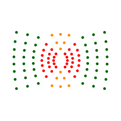
(b)

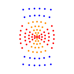
(c)

Figure 8.2: Blocks formed by the zeros of $T_{m,n}^{(\mu)}(\tfrac{1}{2}z^{2})$.

Figures LABEL:root_colour1 and LABEL:root_colour2 show the zeros of $T_{5,8}^{(-57/5)}(\tfrac{1}{2}z^{2})$ and $T_{5,8}^{(-323/20)}(\tfrac{1}{2}z^{2})$ with block E zeros in green, block G in red, block F in orange and block D in blue.

We describe how the roots transition between blocks as a function of $\mu$ and determine the size of each root block for a given $\mu$ when $m=5$ and $n=3$, before stating the result for all $m,n$.

$$\begin{array}[]{c@{\quad}c@{\quad}c}\includegraphics[width=108.405pt]{P5_3m3.pdf}&\includegraphics[width=108.405pt]{P5_3m4.pdf}&\includegraphics[width=108.405pt]{P5_3m5.pdf}\\ \mu=-{\textstyle\frac{16}{5}}&\mu=-{\textstyle\frac{19}{5}}&\mu=-4\\ \includegraphics[width=108.405pt]{P5_3m6.pdf}&\includegraphics[width=108.405pt]{P5_3m8.pdf}&\includegraphics[width=108.405pt]{P5_3m9.pdf}\\ \mu=-{\textstyle\frac{21}{5}}&\mu=-5&\mu=-{\textstyle\frac{26}{5}}\\ \includegraphics[width=108.405pt]{P5_3m11.pdf}&\includegraphics[width=108.405pt]{P5_3m13.pdf}&\includegraphics[width=108.405pt]{P5_3m14.pdf}\\ \mu=-6&\mu=-{\textstyle\frac{34}{5}}&\mu=-7\\ \end{array}$$

Figure 8.3: The roots of $T_{5,3}^{(\mu)}(\tfrac{1}{2}z^{2})$ for $\mu\in[-7,-{\textstyle\frac{16}{5}}].$

$$\begin{array}[]{c@{\quad}c@{\quad}c}\includegraphics[width=108.405pt]{P5_3m16.pdf}&\includegraphics[width=108.405pt]{P5_3m17.pdf}&\includegraphics[width=108.405pt]{P5_3m18.pdf}\\ \mu=-{\textstyle\frac{39}{5}}&\mu=-8&\mu=-{\textstyle\frac{41}{5}}\\ \includegraphics[width=108.405pt]{P5_3m20.pdf}&\includegraphics[width=108.405pt]{P5_3m21.pdf}&\includegraphics[width=108.405pt]{P5_3m23.pdf}\\ \mu=-9&\mu=-{\textstyle\frac{46}{5}}&\mu=-10\\ \includegraphics[width=108.405pt]{P5_3m24.pdf}&\includegraphics[width=108.405pt]{P5_3m26.pdf}&\includegraphics[width=108.405pt]{P5_3m30.pdf}\\ \mu=-{\textstyle\frac{51}{5}}&\mu=-11&\mu=-{\textstyle\frac{61}{5}}\\ \end{array}$$

Figure 8.4: The roots of $T_{5,3}^{(\mu)}(\tfrac{1}{2}z^{2})$ for $\mu\in[-{\textstyle\frac{61}{5}},-{\textstyle\frac{39}{5}}].$

Example 8.3.

Figures 8.3 and 8.4 show the roots of $T_{5,3}^{(\mu)}(\tfrac{1}{2}z^{2})$ for various $\mu$. We describe the root blocks and transitions between the blocks as $\mu$ varies from $-16/5$ to $-61/5$. For $\mu>-4$ the roots form two E-type rectangles of size $6\times 3$ as shown in the first two images in Figure (8.3). As $\mu\to-4$ all roots move towards the imaginary axis. At $\mu=-4$ the innermost column of three zeros from each rectangle have coalesced at the origin and the remaining roots form two rectangles of size $5\times 3$. We discuss the detailed behaviour of the coalesecing zeros in the next section.

As $\mu$ decreases further, the zeros at the origin emerge as a pair of zeros on the imaginary axis and two complex zeros forming a pair of columns of height two. The coalescing roots move away from the origin, while the other roots move towards the origin. As $\mu$ continues to decrease, the zeros that coalesced turn back towards the origin. At $\mu=-5$ these roots and the six roots in the column of the E-rectangle closest to the imaginary axis all coalesce at $z=0$. There are now twelve zeros at the origin and the remaining zeros form two rectangles of size $4\times 3$. As $\mu$ decreases, the roots emerge from the origin as four $2$-triangles with the remaining roots forming two $4\times 3$ E-rectangles. The roots in the triangles initially move away from the origin while the rectangles move towards the origin. For some $\mu\in(-6,-5)$ all the roots in the triangles have turned back towards the origin. At $\mu=-6$ the roots in the triangles and the next innermost column of zeros from each rectangle coalesce at the origin. After the next coalescence, we see the appearance of a a pair of F-trapezoids as well as G-triangles and E-rectangles.

Until all roots coalesce at $\mu=-m-n-1=-9$, the coalescing roots always consist of the roots that previously coalesced plus the innermost column of roots from each E-rectangle. These zeros re-configure and join new blocks as they emerge from the origin. The coalescing roots initially move away from the origin as $\mu$ decreases, and at various values of $\mu$ return to the origin to re-coalesce. For $\mu<-m-n-1$, some of the roots start to form D-type rectangles. Such roots do not return to the origin as $\mu$ decreases, while all other roots return to the origin at each coalesence until they become part of a D-rectangle. The sizes of each root block of $T_{5,3}^{(\mu)}(\tfrac{1}{2}z^{2})$ for $\mu$ between each coalescence point is given in Table 8.2.

$\mu$	E	G	F	D
	rectangle	trapezoid/	triangle/	rectangle
		triangle	trapezoid
$-4<\mu<\infty$	$6\times 3$
$-5<\mu<-4$	$5\times 3$	$2\times 2$	$1$
$-6<\mu<-5$	$4\times 3$	$2\times 1$	$2$
$-7<\mu<-6$	$3\times 3$	2	$3\times 1$
$-8<\mu<-7$	$2\times 3$	2	$4\times 2$
$-9<\mu<-8$	$1\times 3$	2	$5\times 3$
$-10<\mu<-9$		2	$5\times 4$	$6\times 1$
$-11<\mu<-10$		1	$5\times 5$	$6\times 2$
$-\infty<\mu<-11$		$6\times 3$

Table 8.2: Size of the root blocks of $T_{5,3}^{(\mu)}(\tfrac{1}{2}z^{2})$.

Conjecture 8.4.

The block structures when $\mu=-n-j$ for $j=1,\dots,m+n$ and there are roots at the origin are given in Table 8.3. Our investigations suggest the root blocks of $T_{m,n}^{(\mu)}(\tfrac{1}{2}z^{2})$ are as per Table 8.4 for $n>m$ and Table 8.5 for $n\leq m$ for $\mu$ such that $\lceil\mu\rceil=-n-j$ where $j\in\mathbb{Z}$, excluding the points $\mu=-n-1,-n-2,\ldots,-2n-m$.

Condition		Number of zeros	E	D
$j$	$\mu$	at origin	rectangle	rectangle
$1,\ldots,m+1$	$-n-j$	$2nj$	$m-j+1\times n$
$2,\ldots,n$	$-m-n-j$	$2(m+1)(n+1-j)$		$m+1\times j-1$

Table 8.3: Conjectured root blocks of $T_{m,n}^{(\mu)}(\tfrac{1}{2}z^{2})$ at $\mu$ when there are zeros at the origin.

Condition	E	G	F	D
$j=-n-\lceil\mu\rceil$	rectangle	trapezoid/	triangle/	rectangle
		triangle	trapezoid
$j\leq 0$	$m+1\times n$
$1<j<m+1$	$m+1-j\times n$	$n-1\times n-j$	$j$
$m+1<j<n$		$m+n-j\times n-j$	$m$	$m+1\times j-m$
$n<j<m+n$		$m+n-j$	$m\times j-n+1$	$m+1\times j-m$
$j>m+n$				$m+1\times n$

Table 8.4: Conjectured root blocks of $T_{m,n}^{(\mu)}(\tfrac{1}{2}z^{2})$ when $n>m$ and $j=-n-\lceil\mu\rceil\in\mathbb{Z}$.

Condition	E	G	F	D
$j=-n-\lceil\mu\rceil$	rectangle	trapezoid/	trapezoid/	rectangle
		triangle	triangle
$j\leq 0$	$m+1\times n$
$1<j<n$	$m+1-j\times n$	$n-1\times n-j$	$j$
$n+1<j<m+1$	$m+1-j\times n$	$n-1$	$j\times j-n+1$
$m+2<j<m+n$		$m+n-j$	$m\times j-n+1$	$m+1\times j-m$
$j>m+n$				$m+1\times n$

Table 8.5: Conjectured root blocks of $T_{m,n}^{(\mu)}(\tfrac{1}{2}z^{2})$ when $n\leq m$ and $j=-n-\lceil\mu\rceil\in\mathbb{Z}$.

The family of Wronskian Hermite polynomials with partitions $\boldsymbol{\Lambda}=(m^{n})$ are known as the generalised Hermite polynomials $H_{m,n}(z)$. The roots form $m\times n$ rectangles centered on the origin [12, 15].

The appearance of rectangular blocks of width $m+1$ and height $n$ for large positive and negative $k$ in the root pictures for $T_{m,n}^{(-2n-k-1/2)}(\tfrac{1}{2}z^{2})$ is consistent with Theorem 9.6 and Remark 9.7 of [18]. The results therein imply for large $k$ the roots will, up to scaling, be those of a certain Wronskian Hermite polynomial shifted to the right along the real axis, plus the block reflected in the imaginary axis. The numerical investigations in [8] suggest that the relevant Wronskian Hermite polynomial is $H_{m+1,n}(z)$.

8.3 Root coalescences

We now zoom into the origin to investigate precisely how the zeros that coalesce behave as they approach and leave the origin. We start with the example of $T_{5,3}^{(\mu)}(\tfrac{1}{2}z^{2})$, for which the coalescences occur at $\mu=-11,-10,\ldots,-4$.

Example 8.5.

Recall that at $\mu\to-4^{+}$, the six roots of $T_{5,3}^{(\mu)}(\tfrac{1}{2}z^{2})$ that form the two innermost columns of the E-rectangles coalesce at $\mu=-4$. The left-hand plot in Figure 8.5 shows the coalescence of these six zeros by overlaying the root plots for $\mu\in[-4,-16/5]$ near the origin.

$$\begin{array}[]{c@{\quad}c}\includegraphics[width=173.44534pt]{P5_3_nr_m4.pdf}&\includegraphics[width=173.44534pt]{P5_3_second_col_m4_m5.pdf}\\ \mu\in[-4,-{\textstyle\frac{16}{5}}]&\mu\in[-5,-4]\\ \end{array}$$

Figure 8.5: The coalescence of the zeros of $T_{5,3}^{(\mu)}(\tfrac{1}{2}z^{2})$ that are closest to the origin shown by overlaying the zero plots as $\mu$ tends to $\mu=-4$ (left) and $\mu=-5$ (right). The arrows show the direction in which $\mu$ decreases. The solid lines correspond to zeros that arise from the first column of the E-rectangles, and the dashed lines correspond to zeros that arise from the second column of the E-rectangles.

The bold lines in the right-hand plot of Figure 8.5 shows the reapparance of those zeros as $\mu$ decreases towards $\mu=-5$. The previously-real zeros move onto the imaginary axis and the complex zeros return to the complex plane and move away from the origin. The arrows show the direction of decreasing $\mu$. At $\mu\approx 4.2105$, the complex zeros that coalesced turn back towards the origin. The lower solid line in the first quadrant shows the movement of the complex root for $\mu\in(4.2105,-4].$ The upper line shows the root for $\mu\in[-5,4.2105)$. At $\mu\approx 4.32656$, the imaginary zeros also turn back to the origin. The dashed lines show the coalescence of the six zeros in the innermost columns of the E-rectangles for $\mu$ from $-4$ to $-5$. At $\mu=-5$ all twelve zeros are at the origin. The top right plot in Figure 8.6 shows the twelve zeros as they emerge from the origin as $\mu$ decreases from $4$.

$$\begin{array}[]{c@{\quad}c@{\quad}c}\includegraphics[width=108.405pt]{T53_m3m4.pdf}&\includegraphics[width=108.405pt]{T53_m4m5.pdf}&\includegraphics[width=108.405pt]{T53_m5m6.pdf}\\ \mu\in[-4,-3]&\mu\in[-5,-4]&\mu\in[-6,-5]\\ \includegraphics[width=108.405pt]{T53_m6m7.pdf}&\includegraphics[width=108.405pt]{T53_m7m8.pdf}&\includegraphics[width=108.405pt]{T53_m8m9.pdf}\\ \mu\in[-7,-6]&\mu\in[-8,-7]&\mu\in[-9,-8]\\ \includegraphics[width=108.405pt]{T53_m9m10.pdf}&\includegraphics[width=108.405pt]{T53_m10m11.pdf}&\includegraphics[width=108.405pt]{T53_m11m12.pdf}\\ \mu\in[-10,-9]&\mu\in[-11,-10]&\mu\in[-12,-11]\\ \end{array}$$

Figure 8.6: The movement of the roots of $T_{5,3}^{(\mu)}(\tfrac{1}{2}z^{2})$ closest to the origin overlaid for $\mu$ in each given interval.

There are two roots on the imaginary axis, two on the real axis and eight in the complex plane, all of which initially move away from the origin. All roots eventually turn around and return to the origin, along with the next set of six zeros from the innermost column of the E-rectangles. We see the petal-like shapes traced out by the complex zeros as $\mu$ decreases from $-5$ to $-6$. The values of $\mu$ at which each set of zeros turn around are different. The remaining plots in Figure 8.6 show the zeros emerging from the origin and those that coalescence for each of the stated $\mu$. Some roots form F-rectangles when $\mu<-9$.

Our numerical investigations reveal that the angles in the complex plane at which the coalescing roots approach the origin and emerge from it can be determined for all $m,n,j$ where $\mu=-n-j$ and $j=1,2,\ldots,m+n$. Before giving the result for $T_{m,n}^{(\mu)}(z)$ as a function of $z$, we consider an example.

Example 8.6.

The roots of $T_{2,3}^{(\mu)}$ that coalesce at $\mu=-3-j-\varepsilon$ for $j=1\dots,5$ behave as the $n^{\rm th}$ roots of one or minus one as follows:

$$\begin{array}[]{c@{\quad}c@{\quad}c@{\quad}c}j&\mu&\mu\to\mu^{+}&\mu\to\mu^{-}\\ \hline\cr 1&-4&(z^{3}-1)&(z^{3}+1)\\ 2&-5&(z^{4}-1)(z^{2}+1)&(z^{4}+1)(z^{2}-1)\\ 3&-6&(z^{5}-1)(z^{3}+1)(z-1)&(z^{5}+1)(z^{3}-1)(z+1)\\ 4&-7&(z^{4}+1)(z^{2}-1)&(z^{4}-1)(z^{2}+1)\\ 5&-8&(z^{3}-1)&(z^{3}+1)\end{array}$$

Figure 8.7 shows the roots of $T_{2,3}^{(\mu)}$ that converge to to the origin (left) as $\mu\to-4$ and emerge (right) from the origin. The third roots of $1$ and $-1$ are shown in black and red respectively.

$$\begin{array}[]{c@{\quad}c}\includegraphics[width=130.08731pt]{T23_m4in.pdf}&\includegraphics[width=130.08731pt]{T23_m4out}\\ \mu\in[-4,-3]&\mu\in[-5,-4]\\ \end{array}$$

Figure 8.7: The coalescence of the zeros of $T_{2,3}^{(\mu)}$ that are closest to the origin shown by overlaying the zero plots as $\mu$ approaches $\mu=-4$ (left) and $\mu=-5$ (right) from the right. The black arrows (left) indicate the direction of the root movement as $\mu\to-4$ from the right and the red arrows (right) show the roots leaving the origin as $\mu$ decreases from $-4$. The black arrows show the third roots of unity and the red arrows (right) show the third roots of $-1$. The blue lines in the right figure without arrows correspond to the movement of the roots that approach the origin as $\mu\to-5^{-}$ at angles corresponding to the fourth roots of $1$ and the square roots of $-1$.

Conjecture 8.7.

Let $n>m$ and $\varepsilon>0$. For $\mu=-n-j+\varepsilon$ where $j=1,2,\ldots,m+1$ the $nj$ roots of $T_{m,n}^{(\mu)}(z)$ that coalesce at the origin at $\varepsilon=0$ approach the origin on the rays in the complex plane defined by certain roots of $+1$ and $-1$. We encode this behaviour in the polynomial

$$\prod_{k=1}^{j}\left(z^{n+j+1-2k}-(-1)^{n+k}\right),\qquad j=1,2,\ldots,m+1.$$ (8.6)

Furthermore, when $\mu=-n-j+\varepsilon$ for $j=m+2,\ldots,m+n$ the $(m+1)(m+n+1-j)$ roots that approach the origin behave as roots of $\pm 1$ according to

$$\prod_{k=j-m}^{j}\left(z^{n+j+1-2k}-(-1)^{n+k}\right), j=m+2,m+3,\ldots,n,$$ (8.7a)

$$\prod_{k=j-m}^{n}\left(z^{n+j+1-2k}-(-1)^{n+k}\right), j=n+1,n+2,\ldots,m+n.$$ (8.7b)

The roots that coalesce leave the origin on rays that are rotated through $\tfrac{1}{2}\pi$ compared to the coalescence rays. Thus the root behaviours as $\mu=-n-j-\varepsilon$ for $j=1,2,\ldots,m+n$ are encoded in the polynomials

$$\;\;\prod_{k=1}^{j}\left(z^{n+j+1-2k}+(-1)^{n+k}\right), j=1,2,\ldots,m+1,$$ (8.8a)

$$\prod_{k=j-m}^{j}\left(z^{n+j+1-2k}+(-1)^{n+k}\right), j=m+2,m+3,\ldots,n,$$ (8.8b)

$$\prod_{k=j-m}^{n}\left(z^{n+j+1-2k}+(-1)^{n+k}\right), j=n+1,n+2\ldots,m+n.$$ (8.8c)

Similarly, when $n\leq m$ the roots coalesce at and emerge from the origin as $\mu=-n-j\pm\varepsilon$ as roots of $\pm 1$ according to

$$\;\;\prod_{k=1}^{j}\left(z^{n+j+1-2k}\mp(-1)^{n+k}\right), j=1,2\ldots,n,$$ (8.9a)

$$\;\;\prod_{k=1}^{n}\left(z^{n+j+1-2k}\mp(-1)^{n+k}\right), j=n+1,n+2,\ldots,m+1,$$ (8.9b)

$$\prod_{k=j-m}^{n}\left(z^{n+j+1-2k}\mp(-1)^{n+k}\right), j=m+2,m+3,\ldots,m+n.$$ (8.9c)

8.4 The role of the partition

In this section we remark that several features of the generalised Laguerre polynomials can be written in terms of partition data, particularly the hooks of the partition $\boldsymbol{\lambda}=(m+1)^{n}$.

We first propose an expression for the coefficients of the Wronskian Laguerre polynomials $\Omega_{\boldsymbol{\lambda}}^{(\alpha)}(z)$ for all partitions $\boldsymbol{\lambda}$. The result generalises the expression given in Theorem 3 and Proposition 2 in [8] for the coefficients of the Wronskian Hermite polynomials $H_{\boldsymbol{\Lambda}}(z)$ for the subset of partitions $\boldsymbol{\Lambda}$ with $2$-quotient $(\boldsymbol{\lambda},\boldsymbol{\emptyset})$.

Conjecture 8.8.

Consider the Wronskian Laguerre polynomial $\Omega_{\boldsymbol{\lambda}}^{(\alpha)}(z)$ defined in (3.9). Set

$$\Omega_{\boldsymbol{\lambda}}^{(\alpha)}(z)=c_{\boldsymbol{\lambda}}\sum_{j=0}^{|\boldsymbol{\lambda}|}r_{j}^{(\alpha)}\,z^{|\boldsymbol{\lambda}|-j},\$$ (8.10)

with $r_{0}^{(\alpha)}=1$. Then

$$c_{\boldsymbol{\lambda}}=\frac{\Delta_{\boldsymbol{\lambda}}}{\prod_{h\in\boldsymbol{h}_{\boldsymbol{\lambda}}}(-1)^{h}h!}.$$ (8.11)

and

$$r_{j}^{(\alpha)}=\binom{|\boldsymbol{\lambda}|}{j}\sum_{\widetilde{\boldsymbol{\lambda}}<_{j}\,\boldsymbol{\lambda}}\frac{F_{\widetilde{\boldsymbol{\lambda}}}F_{\boldsymbol{\lambda}/\widetilde{\boldsymbol{\lambda}}}}{F_{\boldsymbol{\lambda}}}\frac{\Psi_{\boldsymbol{\lambda}}^{(\alpha)}}{\Psi_{\widetilde{\boldsymbol{\lambda}}}^{(\alpha+\ell(\boldsymbol{\lambda})-\ell(\widetilde{\boldsymbol{\lambda}}))}}\,,$$ (8.12)

where the sum is over all partitions $\widetilde{\boldsymbol{\lambda}}$ in the Young lattice obtained by removing $j$ boxes from the Young diagram of $\boldsymbol{\lambda}$. Moreover,

$$\Psi_{\boldsymbol{\rho}}^{(\alpha)} =(-1)^{|\boldsymbol{\rho}|+\text{ht}(\boldsymbol{\mathrm{P}})}\prod_{j=1}^{\ell(\boldsymbol{\rho})}\Biggl{(}\ \prod_{k=\ell(\boldsymbol{\rho})}^{\boldsymbol{h}_{\boldsymbol{\rho}_{j}}-1}\left(\boldsymbol{h}_{\boldsymbol{\rho}_{j}}-k+\alpha+\ell(\boldsymbol{\rho})\right)$$

$$\quad\quad\quad\quad\quad\quad\quad\times\prod_{k\in\{0,1,\dots,\ell(\boldsymbol{\rho})-1\}\setminus\boldsymbol{h}_{\boldsymbol{\rho}}}^{j-1}\left(j-1-k-\alpha-\ell(\boldsymbol{\rho})\right)\Biggr{)}$$ (8.13)

where $\text{ht}(\boldsymbol{\mathrm{P}})$ is the number of vertical dominoes in the partition $\boldsymbol{\mathrm{P}}$ that has empty 2-core and 2-quotient $(\boldsymbol{\rho},\boldsymbol{\emptyset})$. We remark that $\Psi_{\boldsymbol{\rho}}^{(\alpha)}$ is a polynomial of degree $|\boldsymbol{\rho}|$ in $\alpha$ with leading coefficient $(-1)^{|\boldsymbol{\rho}|}$. A consequence is that all coefficients of the Wronskian Laguerre polynomial are written through (8.13) in terms of the hooks of partitions.

(a) The Young diagram of $\boldsymbol{\Lambda}_{4,3}=(9,8,7,3,2,1)$.

(b) The Young diagram of $\boldsymbol{\Lambda}_{1,3}=(3,2^{4},1)$.

Figure 8.8: Examples of Young diagrams of $\boldsymbol{\Lambda}_{m,n}$ for $m>n-2$ (left) and $m\leq n-2$ (right). The domino tiling is shown. The number of vertical dominoes is $\text{ht}(\boldsymbol{\Lambda}_{4,3})=6$ and $\text{ht}(\boldsymbol{\Lambda}_{1,3})=5$ respectively.

Remark 8.9.

We have also generalised Conjecture 8.8 to determinants of Laguerre polynomials of universal character type [42]. Such polynomials are defined in terms of two partitions and are generalisations of Wronskian Hermite polynomials $H_{\boldsymbol{\Lambda}}(z)$ with $2$-quotient $(\boldsymbol{\lambda}_{1},\boldsymbol{\lambda}_{2})$. Examples include the generalised Umemura polynomials [47] and the Wronskian Laguerre polynomials arising in [9, 21, 22, 26]. A proof of the more general result is under consideration.

We now record some information about the partitions ${\boldsymbol{\lambda}}=((m+1)^{n})$ of the generalised Laguerre polynomial $T_{m,n}^{(\mu)}(z)$ and the corresponding partition $\boldsymbol{\Lambda}_{m,n}$ with empty 2-core and 2-quotient $(\boldsymbol{\lambda},\boldsymbol{\emptyset})$. The Young diagram of $((m+1)^{n})$ is a rectangle of width $m+1$ and height $n$. Since the degree vector of $\boldsymbol{\lambda}$ is

$$\boldsymbol{h}_{\boldsymbol{\lambda}}=(m+n,m+n-1,\ldots,m+1),$$

the Vandermonde determinant is

$$\Delta(\boldsymbol{h}_{\boldsymbol{\lambda}})=(-1)^{n(n-1)/2}\prod_{j=2}^{n}(j-1)!,$$

Since ${\boldsymbol{\lambda}}^{*}=(n^{m+1})$, the multiset of hooks $\mathcal{H}_{m,n}$ of ${\boldsymbol{\lambda}}$ following from (2.3) is

$$\mathcal{H}_{m,n}=\{\{m+n+2-j-k\}_{k=1}^{m+1}\}_{j=1}^{n}\,.$$ (8.14)

The multiset can also be written as

$$\mathcal{H}_{m,n}=\{k^{k}\}_{k=1}^{{\rm min}(m+1,n)-1}\cup\{k^{{\rm min}(m+1,n)}\}_{k={\rm min}(m+1,n)}^{{\rm max}(m+1,n)}\cup\{k^{m+n+1-k}\}_{k={\rm max}(m+1,n)+1}^{m+n}.$$ (8.15)

We now describe the Young diagram of $\boldsymbol{\Lambda}_{m,n}$ and determine its $2$-height. The shape of the Young diagram depends on the relative values of $m$ and $n$. When $m>n-2$, the Young diagram consists of the top $n$ rows of a staircase partition of size $2m+1$ with a complete staircase of size $n$ below. When $m\leq n-2$ the Young diagram consists of the top $m+1$ rows of a $2m+1$ staircase, then $2(n-m-1)$ rows of length $m+1$ and finally a complete $m+1$ staircase. The two cases are illustrated in Figure 8.8.

All Young diagrams corresponding to partitions $\boldsymbol{\Lambda}(0,\boldsymbol{\nu})$ with empty 2-core and 2-quotient $(\boldsymbol{\nu},\boldsymbol{\emptyset})$ have a unique tiling with $|\boldsymbol{\nu}|$ dominoes: tile the boxes of the Young diagram to the right and above the main diagonal with horizontal dominoes and tile the boxes on and below the main diagonal with vertical dominoes. The tiling is illustrated in Figure 8.8. The number of vertical dominoes and, therefore, the $2$-height of $\boldsymbol{\Lambda}(0,\boldsymbol{\nu})$ is

$$\text{ht}(\boldsymbol{\Lambda}(0,\boldsymbol{\nu}))=\sum_{j=1}^{d}(\lambda_{j}^{*}-j)/2,$$

where $d$ is the number of boxes in the main diagonal or, equivalently, the size of the Durfee square. The $2$-heights of the Young diagrams of $\boldsymbol{\Lambda}_{m,n}$ are therefore

$$\text{ht}(\boldsymbol{\Lambda}_{m,n})=\begin{cases}n(n+1)/2&m>n-2\\ (2n-m)(m+1)/2&m\leq n-2.\end{cases}$$ (8.16)

Lemma 8.10.

Recall the expansion (7.1) of the generalised Laguerre polynomial

$$T^{(\mu)}_{\boldsymbol{\lambda}}(z)=c_{m,n}\left(z^{n(m+1)}+d_{1}^{(\mu)}z^{n(m+1)-1}+\dots+(-1)^{n(m+1)}d_{n(m+1)}^{(\mu)})\right)\,.$$

The overall constant is

$$c_{m,n}=(-1)^{n(m+1)}\frac{\Delta(h_{\boldsymbol{\lambda}})}{\prod_{h\in\boldsymbol{h}_{\boldsymbol{\lambda}}}(-1)^{h}\,h!}$$ (8.17)

where

$$\Delta(\boldsymbol{h}_{\boldsymbol{\lambda}})=(-1)^{n(n-1)/2}\prod_{j=1}^{n}(j-1)!,$$ (8.18)

and

$$d_{1}^{(\mu)}=-n(m+1)(\mu+m+n+1)\,.$$ (8.19)

The constant $d_{n(m+1)}^{(\mu)}$ can be written in terms of the hooks of the Young diagram of $\boldsymbol{\lambda}$:

$$d_{n(m+1)}^{(\mu)}=\prod_{h\in\mathcal{H}_{m,n}}\mu+n+h\,.$$ (8.20)

Proof.

Set $\boldsymbol{\lambda}=((m+1)^{n}).$ Then $\ell(\boldsymbol{\lambda})=n$ and $|\boldsymbol{\lambda}|=n(m+1)$. Using the relation (3.10) between $T_{m,n}^{(\mu)}(z)$ and $\Omega_{\boldsymbol{\lambda}}^{(\alpha)}(z)$ and comparing the expansions (7.1) and (8.10), we have

$$c_{m,n}=(-1)^{n(n-1)/2}c_{\boldsymbol{\lambda}},$$

$$d_{1}^{(\mu)}=r_{1}^{(\mu+n)}=n(m+1)\frac{\Psi^{(\mu+n)}_{\boldsymbol{\lambda}}}{\Psi^{(\mu+n)}_{\widetilde{\boldsymbol{\lambda}}}},$$

and

$$d_{n(m+1)}^{(\mu)}=(-1)^{n(m+1)}r_{n(m+1)}^{(\mu+n)}=(-1)^{n(m+1)}\Psi^{(\mu+n)}_{\boldsymbol{\lambda}}\,.$$ (8.21)

The expression for $c_{m,n}$ follows from (8.11) using the degree vector $\boldsymbol{h}_{\boldsymbol{\lambda}}$.

We now determine $\Psi^{(\alpha)}_{\boldsymbol{\lambda}}$ from (8.13). We need (8.16) and

$$\{0,1,\dots n-1\}\setminus\boldsymbol{h}_{\boldsymbol{\lambda}}=\begin{cases}\{0,1,\dots n-1\},\qquad&m>n-2,\\ \{0,1,\dots m\},&m\leq n-2.\end{cases}$$

We deduce that when $m>n-2$ then

$$\Psi_{\boldsymbol{\lambda}}^{(\alpha)} =(-1)^{n(m+1)+n(n+1)/2}\prod_{j=1}^{n}\left(\prod_{k=n}^{m+n-j}\left(m+2n+1-j-k+\alpha\right)\prod_{k=0}^{j-1}\left(j-1-k-\alpha-n\right)\right)$$

$$=(-1)^{n(m+1)}\prod_{j=1}^{n}\left(\prod_{k=1}^{m+1-j}\left(m+n+2-j-k+\alpha\right)\prod_{k=m+2-j}^{m+1}\left(m+n+2-j-k+\alpha\right)\right),$$ (8.22)

where the second line follows after changing variables and taking a minus sign out of each entry in the second set of products. If $m<n-2$ then

$$\Psi_{\boldsymbol{\lambda}}^{(\alpha)} =(-1)^{n(m+1)+(2n-m)(m+1)/2}\prod_{j=1}^{m}\prod_{k=n}^{m+n-j}(m+2n+1-j-k+\alpha)\prod_{j=1}^{n}\prod_{k=0}^{\text{min}(j-1,m)}(j-1-k-\alpha-n)$$

$$=(-1)^{n(m+1)}\prod_{j=1}^{m}\left(\prod_{k=1}^{m+1-j}(m+n+2-j-k+\alpha)\prod_{k=m+2-j}^{m+1}(m+n+2-j-k+\alpha)\right)$$

$$\quad\quad\quad\times\prod_{j=m+1}^{n}\prod_{k=1}^{m+1}(m+n+2-j-k+\alpha)\,.$$ (8.23)

Recalling that the hook in box $(j,k)$ of the Young diagram of $\boldsymbol{\lambda}$ is $h_{j,k}=m+n+2-j-k$, we deduce for all $m,n$ that

$$\Psi_{\boldsymbol{\lambda}}^{(\alpha)}=(-1)^{n(m+1)}\prod_{j=1}^{n}\prod_{k=1}^{m+1}(h_{j,k}+\alpha)\,.$$ (8.24)

Therefore from (8.21) we conclude that

$$d_{n(m+1)}^{(\mu)}=\prod_{j=1}^{n}\prod_{k=1}^{m+1}(h_{j,k}+\mu+n)\,.$$ (8.25)

To determine the coefficient $r_{1}^{(\alpha)}$ we find all partitions $\widetilde{\boldsymbol{\lambda}}$ obtained from $\boldsymbol{\lambda}$ by removing one box from the Young diagram of $\boldsymbol{\lambda}$ such that the result is a valid Young diagram. Since the Young diagram of $\boldsymbol{\lambda}$ is a rectangle, the only possibility is to remove box in position $(n,m+1)$ . Hence

$$\widetilde{\boldsymbol{\lambda}}=((m+1)^{n-1},m),\qquad\boldsymbol{h}_{\widetilde{\boldsymbol{\lambda}}}=(m+n,m+n-1,\dots,m+2,m),$$ (8.26)

and $\ell(\widetilde{\boldsymbol{\lambda}})=n$ and $|\widetilde{\boldsymbol{\lambda}}|=n(m+1)-1$. Clearly $F_{\boldsymbol{\lambda}}=F_{\widetilde{\boldsymbol{\lambda}}}$ and $F_{{\boldsymbol{\lambda}}/{\widetilde{\boldsymbol{\lambda}}}}=1$. We also need the 2-height of the partition $\widetilde{\boldsymbol{\Lambda}}$ with empty 2-core and quotient $(\widetilde{\boldsymbol{\lambda}},\boldsymbol{\emptyset})$. The partition is

$$\widetilde{\boldsymbol{\Lambda}}=\begin{cases}{\left(\{2m-j+1\}_{j=0}^{m},\{m+1\}_{j=1}^{2(n-m-1)-1},m,\{m-j\}_{j=0}^{m-1}\right),}\quad&m\leq n-2,\\[3.0pt] \left(\{2m-j+1\}_{j=0}^{m-1},m,m,\{m-j\}_{j=0}^{m-1}\right),&m=n-1,\\[3.0pt] \left(\{2m-j+1\}_{j=0}^{n-2},\{2m-n\},\{n-j\}_{j=0}^{n-1}\right),&m>n-2,\end{cases}$$ (8.27)

which is obtained from $\boldsymbol{\Lambda}_{m,n}$ by removing one vertical domino from the Young diagram if $m>n-1$ and one horizontal domino if $m\leq n-1$. Hence the 2-height is

$$\text{ht}(\widetilde{\boldsymbol{\Lambda}})=\begin{cases}\tfrac{1}{2}n(n+1)-1,&m>n-2,\\ \tfrac{1}{2}(2n-m)(m+1),\qquad&m\leq n-2.\end{cases}$$ (8.28)

Carefully evaluating (8.13), we deduce that when $m=n-1$ then

$$\Psi_{\widetilde{\boldsymbol{\lambda}}}^{(\alpha)} =-(-1)^{m}\prod_{j=1}^{m}\left(\prod_{k=1}^{m+1-j}\left(2m+3-j-k+\alpha\right)\prod_{k=m+2-j}^{m+1}\left(2m+3-j-k+\alpha\right)\right)$$

$$\quad\quad\quad\times\prod_{j=m+1}^{m+1}\prod_{k=2}^{m+1}(2m+3-j-k+\alpha)\,.$$ (8.29)

When $m>n-2$ then

$$\Psi_{\widetilde{\boldsymbol{\lambda}}}^{(\alpha)} =-(-1)^{n(m+1)}\prod_{j=1}^{n-1}\prod_{k=1}^{m+1-j}(m+n+2-j-k+\alpha)\prod_{k=2}^{m+1-n}(m+n+2-(n)-k+\alpha)$$

$$\quad\quad\times\prod_{j=1}^{n}\prod_{k=m+2-j}^{m+1}(m+n+2-j-k+\alpha),$$ (8.30)

and when $m\leq n-2$ then

$$\Psi_{\widetilde{\boldsymbol{\lambda}}}^{(\alpha)} =-(-1)^{n(m+1)}\prod_{j=1}^{n-1}\prod_{k=1}^{m+1-j}(m+n+2-j-k+\alpha)\prod_{j=1}^{m}\prod_{k=m+2-j}^{m+1}(m+n+2-j-k+\alpha)$$

$$\quad\quad\times\prod_{j=m}^{n-1}\prod_{k=3}^{m+2}(m+n+2-j-k+\alpha)\prod_{j=m+1}^{n-1}\prod_{k=1}^{1}(m+n+2-j-k+\alpha).$$ (8.31)

We notice that in each case $\Psi_{\widetilde{\boldsymbol{\lambda}}}^{(\alpha)}$ includes all terms of the form $h_{j,k}+\alpha$ where $h_{j,k}$ are the hooks of the Young diagram of $\boldsymbol{\lambda}$ except for the term $m+1+\alpha$. Therefore

$$(m+1+\alpha)\Psi_{\widetilde{\boldsymbol{\lambda}}}^{(\alpha)}=-(-1)^{n(m+1)}\prod_{j=1}^{n}\prod_{k=1}^{m+1}(h_{j,k}+\alpha)=-\Psi_{\boldsymbol{\lambda}}^{(\alpha)}\,.$$ (8.32)

We conclude that

$$r_{1}^{(\alpha)}=n(m+1)\frac{\Psi_{\boldsymbol{\lambda}}^{(\alpha)}}{\Psi_{\widetilde{\boldsymbol{\lambda}}}^{(\alpha)}}=-n(m+1)(\alpha+m+1)\,.$$ (8.33)

and

$$d_{1}^{(\alpha)}=-n(m+1)(\mu+m+n+1)\,.$$ (8.34)

∎

Conjecture 8.11.

The hook multiset $\mathcal{H}_{m,n}$ (8.15) has the form

$$\mathcal{H}_{m,n}=\begin{cases}\{k^{p_{1}}\}_{k=1}^{m}\cup\{k^{p_{2}}\}_{k=m+1}^{n}\cup\{k^{p_{3}}\}_{k=n+1}^{m+n},\qquad&n>m,\\[3.0pt] \{k^{p_{1}}\}_{k=1}^{n}\cup\{k^{\widetilde{p}_{2}}\}_{k=n+1}^{m+1}\cup\{k^{p_{3}}\}_{k=m+2}^{m+n},\qquad&n\leq m,\end{cases}$$ (8.35)

where

$$p_{1}=k\quad,\quad p_{2}=m+1\quad,\quad\widetilde{p}_{2}=n\quad,\quad p_{3}=m+n+1-k,$$

are the multiplicities of the hooks in each respective set. The discriminant of $T_{m,n}^{(\mu)}(z)$ for $n>m$ in terms of partition data is

$$\text{Dis}_{m,n}(\mu) =(-1)^{(m+1)\lfloor n/2\rfloor}c_{m,n}^{n(m+1)-1}$$

$$\qquad\times\prod_{k=1}^{m}k^{2k(n-k)(k-1-m)}\prod_{k=1}^{m}k^{kp_{1}^{2}}\,(\mu+n+k)^{f(n-1,p_{1})}$$

$$\qquad\times\prod_{k=m+1}^{n}k^{kp_{2}^{2}}\,(\mu+n+k)^{f(m+n-k,p_{2})}\prod_{k=n+1}^{m+n}k^{kp_{3}^{2}}\,(\mu+n+k)^{f(m,p_{3})},$$ (8.36)

where $f(k,p)=kp^{2}-p(p-1)(p-2)/3$. Similarly the discriminant when $n\leq m$ is

$$\text{Dis}_{m,n}(\mu) =(-1)^{(m+1)\lfloor n/2\rfloor}c_{m,n}^{2(n(m+1)-1)}\prod_{k=1}^{m}k^{2k(n-k)(k-1-m)}\prod_{k=1}^{n}k^{kp_{1}^{2}}\,(\mu+n+k)^{f(n-1,p_{1})}$$

$$\qquad\times\prod_{k=n+1}^{m}k^{k\widetilde{p}_{2}^{2}}\,(\mu+n+k)^{f(k-1,\widetilde{p}_{2})}\prod_{k=m+1}^{m+n}k^{kp_{3}^{2}}\,(\mu+n+k)^{f(m,p_{3})}.$$ (8.37)

The discriminant representations (8.36) and (8.37) follow directly from rewriting (8.3) and (8.4) in terms of the hooks and their multiplicities as defined by (8.35).

As already mentioned, the E- and F-type blocks seen for large positive and negative values of $\mu$ are of size $m+1\times n$ and therefore resemble the rectangular Young diagram of $\lambda$. Moreover, the three allowed sets of block structures corresponding to intermediate values of $\mu$, as given in table 8.4, appear at $\mu+n+k=0$ where the multiplicity of the first column hook $k$ in $\boldsymbol{h}_{\boldsymbol{\lambda}}$ changes its multiplicity type from type $p_{1}$ to $p_{2}$ to $p_{3}$.

Conjecture 8.12.

Finally, the set of integers encoding the $n^{\rm th}$ roots of $\pm 1$ via the polynomials in Conjecture 8.7 are the hooks on the diagonals parallel to the main diagonal of the Young diagram of $\boldsymbol{\lambda}$. Specifically, as $\varepsilon\to 0$ for $\mu=-n-j-\varepsilon$, hook $h_{jk}$ in column $j$ contributes an $h_{jk}^{\rm th}$ root of unity if $k$ is odd and an $h_{jk}^{\rm th}$ root of $-1$ if $k$ is even. For $\mu=-n-j\mp\varepsilon$ the polynomials in Conjecture 8.7 are

$$\ \ \prod_{k=1}^{j}\ \ z^{h_{j,k}}\mp(-1)^{n+k}, j=1,2,\dots,m+1,$$

$$\prod_{k=j-m}^{n}z^{h_{j,k}}\mp(-1)^{n+k}, j=m+2,m+3,\dots,n,$$

$$\prod_{k=j-m}^{n}z^{h_{j,k}}\mp(-1)^{n+k}, j=n+1,n+2,\dots,m+n,$$

when $n>m$ where $h_{j,k}\in\mathcal{H}_{m,n}$. For $n\leq m$ the result is

$$\ \ \prod_{k=1}^{j}z^{h_{j,k}}\mp(-1)^{n+k}, j=1,2,\dots,n,$$

$$\ \ \prod_{k=1}^{n}z^{h_{j,k}}\mp(-1)^{n+k}, j=n+1,n+2,\dots,m+1,$$

$$\prod_{k=j-m}^{n}z^{h_{j,k}}\mp(-1)^{n+k}, j=m+2,m+3,\dots,m+n.$$

Remark 8.13.

The result follows from Conjecture 8.7 by rewriting the hook multiset (8.15) as

$$\mathcal{H}_{m,n}=\begin{cases}\{\{n{+}j{+}1{-}2k\}_{k=1}^{j}\}_{j=1}^{m+1}\cup\{\{n{+}j{+}1{-}2k\}_{k=j-m}^{j}\}_{j=m+2}^{n}\cup\{\{n{+}j{+}1{-}2k\}_{k=j-m}^{n}\}_{j=n+1}^{m+n},&n>m,\\ \{\{n{+}j{+}1{-}2k\}_{k=1}^{j}\}_{j=1}^{n}\cup\{\{n{+}j{+}1{-}2k\}_{k=1}^{n}\}_{j=n+1}^{m+1}\cup\{\{n{+}j{+}1{-}2k\}_{k=j-m}^{n}\}_{j=m+2}^{m+n},&n\leq m.\end{cases}$$ (8.38)

We illustrate how to determine the root angle polynomials from a Young diagram in Figure 8.9 for the example 8.6 of $T_{2,3}^{(\mu)}(z)$.

Remark 8.14.

We have found other families of Wronskian Hermite and Wronskian Laguerre polynomials for which properties can be written compactly in terms of partition data. Combinatorial concepts also appeared in the studies of special polynomials associated with Painlevé equations in [67, 68, 69, 50, 8, 7]. We are currently investigating this curious appearance of partition combinatorics in various aspects of Wronskian polynomials.

Figure 8.9: The hooks on the $j^{\rm th}$ diagonal of the Young diagram of $T_{2,3}^{(\mu)}$ encode the behaviour of the roots that coalesce at the origin at $\mu=-n-j-\varepsilon$ through the polynomials in Conjecture 8.12. When $j=3$ the polynomial is $(z^{5}-1)(z^{3}+1)(z-1)$ and when $j=3$ or $j=5$ the polynomial is $z^{3}-1$.

Acknowledgements

We thank David Gómez-Ullate, Davide Masoero and Bryn Thomas for helpful comments and illuminating discussions. We also thank the reviewers for their constructive comments and suggestions.

References

- [1] V.E. Adler, Nonlinear chains and Painlevé equations, Physica, D73 (1994) 335–351.
- [2] T. Amdeberhan, Discriminants of Umemura polynomials associated to Painlevé III, Phys. Lett A., 354 (2006) 410–413.
- [3] H. Aratyn, J.F. Gomes, G.V. Lobo and A.H. Zimerman, On Rational Solutions of Dressing Chains of Even Periodicity, Symmetry, 15 (2023) 249.
- [4] H. Aratyn, J.F. Gomes, G.V. Lobo and A.H. Zimerman, Why is my rational Painlevé V solution not unique?, arXiv:2307.07825 [nlin.SI].
- [5] H. Aratyn, J.F. Gomes, G.V. Lobo and A.H. Zimerman, Two-fold degeneracy of a class of rational Painlevé V solutions, arXiv:2310.01585 [nlin.SI].
- [6] E. Basor, P. Bleher, R. Buckingham, T. Grava, A. Its, E. Its and J.P. Keating, A representation of joint moments of CUE characteristic polynomials in terms of Painlevé functions, Nonlinearity, 32 (2019) 4033–4078.
- [7] N. Bonneux, Asymptotic behavior of Wronskian polynomials that are factorized via -cores and -quotients, Math. Phys., Anal. and Geom., 23 (2020) 36.
- [8] N. Bonneux, C. Dunning and M. Stevens, Coefficients of Wronskian Hermite polynomials, Stud. Appl. Math., 144 (2020) 245–288.
- [9] N. Bonneux and A.B.J. Kuijlaars, Exceptional Laguerre polynomials, Stud. Appl. Math., 141 (2018) 547–595.
- [10] N. Bonneux and M. Stevens, Recurrence relations for Wronskian Laguerre polynomials, Integral Transforms Spec. Funct., 32 (2021) 39–406.
- [11] P.A. Clarkson, The third Painlevé equation and associated special polynomials, J. Phys. A, 36 (2003) 9507–9532.
- [12] P.A. Clarkson, The fouth Painlevé equation and associated special polynomials, J. Math. Phys., 44 (2003) 5350–5374.
- [13] P.A. Clarkson, Special polynomials associated with rational solutions of the fifth Painlevé equation, J. Comp. Appl. Math., 178 (2005) 111–129.
- [14] P.A. Clarkson, Painlevé equations – nonlinear special functions, in: Orthogonal Polynomials and Special Functions: Computation and Application, F. Màrcellan and W. Van Assche (Editors), Lect. Notes Math., vol. 1883, Springer-Verlag, Berlin, pp. 331–411, 2006.
- [15] P.A. Clarkson, Special polynomials associated with rational solutions of the Painlevé equations and applications to soliton equations, Comput. Methods Funct. Theory, 6 (2006) 329–401.
- [16] P.A. Clarkson, Recurrence coefficients for discrete orthonormal polynomials and the Painlevé equations, J. Phys. A, 46 (2013) 185205.
- [17] P.A. Clarkson, Classical solutions of the degenerate fifth Painlevé equation, J. Phys. A, 56 (2023) 134002.
- [18] R. Conti and D. Masoero, Counting monster potentials, J. High Energ. Phys., 02 (2021) 059.
- [19] C.L. Dodgson, IV. Condensation of determinants, being a new and brief method for computing their arithmetical values, Proc. R. Soc. Lond., 15 (1866) 150–155.
- [20] A.J. Durán, Exceptional Charlier and Hermite orthogonal polynomials, J. Approx Theory, 182 (2014) 29–58.
- [21] A.J. Durán, Exceptional Meixner and Laguerre orthogonal polynomials, J. Approx Theory., 184 (2014) 176–208.
- [22] A.J. Durán and M. Pérez, Admissibility condition for exceptional Laguerre polynomials, J. Math. Anal. Appl., 424 (2015) 1042–1053.
- [23] A.S. Fokas and M.J. Ablowitz, On a unified approach to transformations and elementary solutions of Painlevé equations, J. Math. Phys., 23 (1982) 2033–2042.
- [24] P.J. Forrester and N.S. Witte, Application of the -function theory of Painlevé equations to random matrices: PIV, PII and the GUE, Commun. Math. Phys., 219 (2001) 357–398.
- [25] P.J. Forrester and N.S. Witte, Application of the -function theory of Painlevé equations to random matrices: PV, PIII, the LUE, JUE, and CUE, Comm. Pure Appl. Math, 55 (2002) 679–727.
- [26] D. Gómez-Ullate, Y. Grandati and R. Milson, Shape invariance and equivalence relations for pseudo-Wronskians of Laguerre and Jacobi polynomials, J. Phys. A, 51 (2018) 345201.
- [27] D. Gómez-Ullate, Y. Grandati and R. Milson, Rational solutions of Painlevé systems, in: Nonlinear Systems and Their Remarkable Structures. Vol. 2, N. Euler and M.C. Nucci (Editors), Chapman and Hall/CRC Press, Boca Raton, FL, USA, pp. 249–293, 2019. [arXiv:2009.11668]
- [28] D. Gómez-Ullate, Y. Grandati, S. Lombardo and R. Milson, Rational solutions of dressing chains and higher order Painlevé systems, arXiv:1811.10186 [math-ph].
- [29] V.I. Gromak, I. Laine and S. Shimomura, Painlevé Differential Equations in the Complex Plane, Studies in Math., vol. 28, de Gruyter, Berlin, New York, 2002.
- [30] V.I. Gromak and N.A. Lukashevich, Special classes of solutions of Painlevé’s equations, Diff. Eqns., 18 (1982) 317–326.
- [31] G. James and A. Kerber, The Representation Theory of the Symmetric Group, Vol. 16, Encyclopedia of Mathematics and its Applications, Addison-Wesley Publishing Co., Reading, Mass, 1981.
- [32] M. Jimbo and T. Miwa, Monodromy preserving deformations of linear ordinary differential equations with rational coefficients. II, Physica, D2 (1981) 407–448.
- [33] E.L. Ince, Ordinary Differential Equations, Dover, New York, 1956.
- [34] K. Iwasaki, H. Kimura, S. Shimomura and M. Yoshida, From Gauss to Painlevé: a Modern Theory of Special Functions, Aspects of Mathematics E, vol. 16, Vieweg, Braunschweig, Germany, 1991.
- [35] K. Kajiwara and T. Masuda, A generalization of determinant formulae for the solutions of Painlevé II and XXXIV equations, J. Phys. A, 32 (1999) 3763–3778.
- [36] K. Kajiwara and T. Masuda, On the Umemura polynomials for the Painlevé III equation, Phys. Lett. A, 260 (1999) 462–467.
- [37] K. Kajiwara and Y. Ohta, Determinantal structure of the rational solutions for the Painlevé II equation, J. Math. Phys., 37 (1996) 4393–4704.
- [38] K. Kajiwara and Y. Ohta, Determinant structure of the rational solutions for the Painlevé IV equation, J. Phys. A, 31 (1998) 2431–2446.
- [39] K. Kajiwara, Y. Ohta, J. Satsuma, B. Grammaticos and A. Ramani, Casorati determinant solutions for the discrete Painlevé-II equation, J. Phys. A, 27 (1994) 915–922.
- [40] K. Kajiwara, K. Yamamoto and Y. Ohta, Rational solutions for the discrete Painlevé II equation, Phys. Lett. A, 232 (1997) 189–199.
- [41] A.V. Kitaev, C.K. Law and J.B. McLeod, Rational solutions of the fifth Painlevé equation, Diff. Int. Eqns., 7 (1994) 967–1000.
- [42] K. Koike, On the decomposition of tensor products of the representations of the classical groups: By means of the universal characters, Adv. Math., 74 (1989) 57–86.
- [43] A.B.J. Kuijlaars, and K.T.R. McLaughlin, Riemann-Hilbert Analysis for Laguerre Polynomials with Large Negative Parameter, Comput. Methods Funct. Theory, 1 (2001) 205–233.
- [44] I.G. Macdonald, Symmetric Functions and Hall Polynomials, Oxford Mathematical Monographs, Oxford University Press, Oxford, 1995.
- [45] T. Masuda, Classical transcendental solutions of the Painlevé equations and their degeneration, Tohoku Math. J., 56 (2004) 467–490.
- [46] T. Masuda, Special polynomials associated with the Noumi-Yamada system of type , Funkcial. Ekvac., 48 (2005) 231–246.
- [47] T. Masuda, Y. Ohta and K. Kajiwara, A determinant formula for a class of rational solutions of Painlevé V equation, Nagoya Math. J., 168 (2002) 1–25.
- [48] T. Muir, A Treatise on the Theory of Determinants (Revised and enlarged by William H. Metzler), Dover, New York, 1960.
- [49] M. Noumi, Painlevé Equations through Symmetry, Trans. Math. Mono., vol. 223, Amer. Math. Soc., Providence, RI, 2004.
- [50] M. Noumi, Notes on Umemura polynomials, Ann. Fac.Sci. Toulouse Maths., 5 (2020) 1091–1118.
- [51] M. Noumi and Y. Yamada, Affine Weyl groups, discrete dynamical systems and Painlevé equations, Commun. Math. Phys., 199 (1998) 281–295.
- [52] M. Noumi and Y. Yamada, Umemura polynomials for the Painlevé V equation, Phys. Lett. A, 247 (1998) 65–69.
- [53] M. Noumi and Y. Yamada, Higher order Painlevé equations of type , Funkcial. Ekvac., 41 (1998) 483–503.
- [54] M. Noumi and Y. Yamada, Symmetries in the fourth Painlevé equation and Okamoto polynomials, Nagoya Math. J., 153 (1999) 53–86.
- [55] M. Noumi and Y. Yamada, Symmetries in Painlevé equations, Sugaku Expositions, 17 (2004) 203–218.
- [56] K. Okamoto, Polynomial Hamiltonians associated with Painlevé equations. I, Proc. Japan Acad. Ser. A Math. Sci., 56 (1980) 264–268; 367–371.
- [57] K. Okamoto, Studies on the Painlevé equations III. Second and fourth Painlevé equations, PII and PIV, Math. Ann., 275 (1986) 221–255.
- [58] K. Okamoto, Studies on the Painlevé equations. II. Fifth Painlevé equation PV, Japan. J. Math., 13 (1987) 47–76.
- [59] K. Okamoto, Studies on the Painlevé equations I. Sixth Painlevé equation PVI, Ann. Mat. Pura Appl., 146 (1987) 337–381.
- [60] K. Okamoto, Studies on the Painlevé equations IV. Third Painlevé equation PIII, Funkcial. Ekvac, 30 (1987) 305–332.
- [61] K. Okamoto and Y. Ohyama, Mathematical works of Hiroshi Umemura, Ann. Fac. Sci. Toulouse Math. (6), 29 (2020) 1053–1062.
- [62] F.W.J. Olver, A.B. Olde Daalhuis, D.W. Lozier, B.I. Schneider, R.F. Boisvert, C.W. Clark, B.R. Miller, B.V. Saunders, H.S. Cohl, and M.A. McClain (Editors), NIST Digital Library of Mathematical Functions, http://dlmf.nist.gov/, Release 1.1.11 (September 15, 2023).
- [63] D.P. continues to , Discriminants of some Painlevé polynomials, in: Number Theory for the Millennium, III, M.A. Bennett, B.C. Berndt, N. Boston, H.G. Diamond, A.J. Hildebrand and W. Philipp (Editors), A K Peters, Natick, MA, pp. 205–221, 2003.
- [64] R.P. Stanley, Enumerative Combinatorics, Vol. 2, Cambridge Studies in Advanced Mathematics, 62, Cambridge University Press, Cambridge, 1999.
- [65] J.J. Sylvester, Sur une classe nouvelle d’equations differéntielles et déquations aux differences finies d’une forme intégrable, Compt. Rend. Acad. Sc., 54 (1862) 129–170.
- [66] T. Tsuda, Universal characters, integrable chains and the Painlevé equations, Adv. Math., 197 (2005) 587–606.
- [67] H. Umemura, Painlevé equations and classical functions, Sugaku Expositions, 11 (1998) 77–100.
- [68] H. Umemura, Painlevé equations in the past 100 Years, A.M.S. Translations, 204 (2001) 81–110.
- [69] H. Umemura, Special polynomials associated with the Painlevé equations I, Ann. Fac. Sci. Toulouse Math. (6), 29 (2020) 1063–1089.
- [70] P.R. Vein and P. Dale, Determinants and Their Applications in Mathematical Physics, Springer-Verlag, New York, 1999.
- [71] A.P. Veselov and A.B. Shabat, A dressing chain and the spectral theory of the Schrödinger operator, Funct. Anal. Appl., 27 (1993) 1–21.
- [72] A.P. Vorob’ev, On rational solutions of the second Painlevé equation, Diff. Eqns., 1 (1965) 58–59.
- [73] H. Watanabe, Solutions of the fifth Painlevé equation I, Hokkaido Math. J., 24 (1995) 231–267.
- [74] M. Wildon, Counting partitions on the abacus, Ramanujan J., 17 (2008) 355–367.
- [75] Y. Yamada, Special polynomials and generalized Painlevé equations, in: Combinatorial Methods in Representation Theory, K. Koike, M. Kashiwara, S. Okada, I. Terada and H.F. Yamada (Editors), Adv. Stud. Pure Math., 28, Kinokuniya, Tokyo, Japan, pp. 391–400, 2000.
- [76] A.I. Yablonskii, On rational solutions of the second Painlevé equation, Vesti Akad. Navuk. BSSR Ser. Fiz. Tkh. Nauk., 3 (1959) 30–35.