Types and stability of fixed points for positivity-preserving discretized dynamical systems in two dimensions

Shousuke Ohmori^1,∗) and Yoshihiro Yamazaki²

¹National Institute of Technology, Gunma College, Maebashi-shi, Gunma 371-8530, Japan
²Department of Physics, Waseda University, Shinjuku, Tokyo 169-8555, Japan

*corresponding author: 42261timemachine@ruri.waseda.jp
  

Abstract
Relationship for dynamical properties in the vicinity of fixed points between two-dimensional continuous and its positivity-preserving discretized dynamical systems is studied. Based on linear stability analysis, we reveal the conditions under which the dynamical structures of the original continuous dynamical systems are retained in their discretized dynamical systems, and the types of fixed points are identified if they change due to discretization. We also discuss stability of the fixed points in the discrete dynamical systems. The obtained general results are applied to Sel’kov model and Lengyel-Epstein model.

1 Introduction

Many studies have been conducted on the dynamical properties of ultradiscrete equations derived from continuous differential equations for non-integrable systems, such as reaction-diffusion systems[1, 2, 3], an inflammatory response system[4, 5] and a biological negative-feedback system[6]. For these derivations, it is necessary to adopt a difference method that preserves the positivity of the continuous equations in order to apply the ultradiscrete limit[7]. As one of the positivity-preserving difference methods, the tropical discretization method[1] is often applied. Then, understanding correspondence of dynamical properties among original continuous differential equations, their tropically discretized equations and their ultradiscretized equations is important, and whether the derived discrete equations can retain the dynamical properties of the original models is a significant problem.

With the above problem in mind, we have recently studied dynamical properties of the local bifurcations (transcritical, saddle-node, pitchfork) in one-dimensional dynamical systems[8, 9]. In these previous studies, we argued stabilities of fixed points in continuous differential equations and their tropically discretized ones. We successfully identified conditions under which the derived discrete dynamical systems can retain the bifurcations of the original continuous ones via tropical discretization.

In this letter, we focus on types and stability of fixed points in two-dimensional dynamical systems. So far, we have numerically investigated Sel’kov model as a specific example[10, 11, 12]. However, the previous studies have not been treated as generally and analytically as in the above one-dimensional case. Moreover in two-dimensional dynamical systems, there is an essential difference from the one-dimensional case: existence of Hopf (or Neimark-Sacker) bifurcation. Therefore, in addition to the general treatment of one-dimensional cases, that of two-dimensional cases is meaningful and important.

2 General results

Now we consider the following continuous two-dimensional differential equation with positive variables ${\mathbf{x}}=(x_{1},x_{2})$

$$\frac{d\mathbf{x}}{dt} =\mathbf{F}(\mathbf{x})=\mathbf{f}(\mathbf{x})-\mathbf{g}(\mathbf{x}),$$ (1)

where $x_{1},x_{2}>0$ and we assume that $\mathbf{F}(\mathbf{x})$ can be divided into two positive smooth functions $\mathbf{f}=(f_{1},f_{2})$ and $\mathbf{g}=(g_{1},g_{2})$. By the tropical discretization[1], we obtain the following discrete dynamical system from eq.(1):

$$\mathbf{x}_{n+1}=\mathbf{x}_{n}\frac{\mathbf{x}_{n}+\tau\mathbf{f}(\mathbf{x}_{n})}{\mathbf{x}_{n}+\tau\mathbf{g}(\mathbf{x}_{n})},$$ (2)

where $\tau(>0)$ and $n$ show the discretized time interval and the number of iteration steps with non-negative integer; $\mathbf{x}_{n}=\mathbf{x}(n\tau)$, respectively. It is found that if $\bar{\mathbf{x}}=(\bar{x}_{1},\bar{x}_{2})$ is a fixed point of eq.(1), then $\bar{\mathbf{x}}$ also becomes a fixed point of eq.(2). Hereafter the fixed points $\bar{\mathbf{x}}$ of eqs.(1) and (2) are denoted by $\bar{\mathbf{x}}^{(c)}$ and $\bar{\mathbf{x}}^{(d)}$, respectively, when their difference is needed to be made clear. We set the Jacobian $\mathbf{J(\bar{\mathbf{x}})}=\begin{pmatrix}D_{11}&D_{12}\\ D_{21}&D_{22}\\ \end{pmatrix}$ at $\bar{\mathbf{x}}^{(c)}$, where $D_{ij}=\displaystyle\frac{\partial{(f_{i}-g_{i})}}{\partial{x_{j}}}(\bar{\mathbf{x}})$ ($i,j=1,2$). The trace $T$ and the determinant $\Delta$ of $\mathbf{J(\bar{\mathbf{x}})}$ is obtained as $T=D_{11}+D_{22}$ and $\Delta=D_{11}D_{22}-D_{12}D_{21}$. The Jacobian of eq.(2) is also given by $\mathbf{J_{\tau}(\bar{\mathbf{x}})}=\begin{pmatrix}1+Z_{\tau 1}D_{11}&Z_{\tau 1}D_{12}\\ Z_{\tau 2}D_{21}&1+Z_{\tau 2}D_{22}\\ \end{pmatrix}$, where $Z_{\tau i}\equiv\displaystyle\frac{\tau\bar{x}_{i}}{\bar{x}_{i}+\tau\bar{f}_{i}}~{}(>0)$ and $\bar{f}_{i}\equiv f_{i}(\bar{\mathbf{x}})$ ($i=1,2$). Note that the trace $T^{\prime}$ and the determinant $\Delta^{\prime}$ of $\mathbf{J_{\tau}(\bar{\mathbf{x}})}$ are given as

$$T^{\prime} = 2+\displaystyle\frac{\tau\bar{x}_{1}\bar{x}_{2}T+\tau^{2}(\bar{x}_{1}\bar{f}_{2}D_{11}+\bar{x}_{2}\bar{f}_{1}D_{22})}{(\bar{x}_{1}+\tau\bar{f}_{1})(\bar{x}_{2}+\tau\bar{f}_{2})},$$

$$\Delta^{\prime} = T^{\prime}-1+Z_{\tau 1}Z_{\tau 2}\Delta.$$ (3)

2.1 Type of the fixed point

Focusing on the sign of $\Delta$, we determine relationship of the three types of fixed points (saddle, node, spiral) between in two dimensional continuous and discrete dynamical systems[13, 14]. (i) When $\Delta<0$, $\bar{\mathbf{x}}^{(c)}$ becomes a saddle. From eq.(3), $\Delta^{\prime}<T^{\prime}-1$ holds. Then, $\bar{\mathbf{x}}^{(d)}$ becomes either a saddle or an unstable node. In fact, $\bar{\mathbf{x}}^{(d)}$ becomes saddle when $\Delta^{\prime}>-T^{\prime}-1$, otherwise unstable node. Expressing $T^{\prime}$ and $\Delta^{\prime}$ in terms of $\tau$, we have the quadratic inequality corresponding to $\Delta^{\prime}>-T^{\prime}-1$,

$$P_{sd}(\tau)\equiv A_{sd}\tau^{2}+B_{sd}\tau+C_{sd}>0,$$ (4)

where

$$A_{sd} = 2(\bar{x}_{1}\bar{f}_{2}D_{11}+\bar{x}_{2}\bar{f}_{1}D_{22})+\bar{x}_{1}\bar{x}_{2}\Delta+4\bar{f}_{1}\bar{f}_{2},$$

$$B_{sd} = 2\bar{x}_{1}\bar{x}_{2}T+4(\bar{x}_{1}\bar{f}_{2}+\bar{x}_{2}\bar{f}_{1}),$$ (5)

$$C_{sd} = 4\bar{x}_{1}\bar{x}_{2}\;\;\;(>0).$$

By using $P_{sd}(\tau)$, the above statement can be rewritten as follows; $\bar{\mathbf{x}}^{(d)}$ becomes saddle for $P_{sd}(\tau)>0$ and unstable node for $P_{sd}(\tau)<0$ when $\Delta<0$. (ii) In the case of $\Delta>0$, the fixed point $\bar{\mathbf{x}}^{(c)}$ becomes node when $4\Delta<T^{2}$ and spiral when $4\Delta>T^{2}$. From $\Delta>0$, we obtain $\Delta^{\prime}>T^{\prime}-1$ based on eq.(3). In this case, the fixed point $\bar{\mathbf{x}}^{(d)}$ can be classified as follows. (ii-a) When $P_{sd}(\tau)>0$ and $4\Delta^{\prime}<{T^{\prime}}^{2}$, $\bar{\mathbf{x}}^{(d)}$ becomes node. Note that the inequality $4\Delta^{\prime}<{T^{\prime}}^{2}$ is transformed into the following quadratic inequality with respect to $\tau$ by eq.(3):

$$P_{nd}(\tau)\equiv A_{nd}\tau^{2}+B_{nd}\tau+C_{nd}>0,$$ (6)

where

$$A_{nd} = (\bar{x}_{1}\bar{f}_{2}D_{11}+\bar{x}_{2}\bar{f}_{1}D_{22})^{2}-4\bar{x}_{1}\bar{x}_{2}\bar{f}_{1}\bar{f}_{2}\Delta,$$

$$B_{nd} = 2\bar{x}_{1}\bar{x}_{2}T(\bar{x}_{1}\bar{f}_{2}D_{11}+\bar{x}_{2}\bar{f}_{1}D_{22})$$ (7)

$$-4\bar{x}_{1}\bar{x}_{2}(\bar{x}_{1}\bar{f}_{2}+\bar{x}_{2}\bar{f}_{1})\Delta,$$

$$C_{nd} = (\bar{x}_{1}\bar{x}_{2})^{2}(T^{2}-4\Delta).$$

(ii-b) When $P_{sd}(\tau)>0$ and $4\Delta^{\prime}>{T^{\prime}}^{2}$, or $P_{nd}(\tau)<0$, $\bar{\mathbf{x}}^{(d)}$ becomes spiral. (ii-c) When $P_{sd}(\tau)<0$, $P_{nd}(\tau)>0$ automatically holds and $\bar{\mathbf{x}}^{(d)}$ becomes saddle. In summary, the type of the fixed point $\bar{\mathbf{x}}^{(d)}$ can be determined depending on the sign of $\Delta$, $P_{sd}(\tau)$, and $P_{nd}(\tau)$ as shown in Fig.1. Note that $P_{nd}(\tau)>0$ automatically holds for any $\tau$ when $\Delta<0$. In a simpler way, the type of $\bar{\mathbf{x}}^{(d)}$ can be determined according to the flowchart shown in Fig.2.

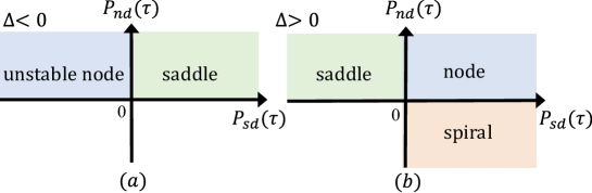
Figure 1: Classifications of the type of the fixed point in eq.(2), $\bar{\mathbf{x}}^{(d)}$. (a) $\Delta<0$. (b) $\Delta>0$.

Figure 2: Flowchart for obtaining the type of $\bar{\mathbf{x}}^{(d)}$.

2.2 Stability

Here we consider the stability of $\bar{\mathbf{x}}^{(d)}$. Assuming $\Delta^{\prime}>\pm T^{\prime}-1$, the fixed point $\bar{\mathbf{x}}^{(d)}$ becomes stable when the inequality $T^{\prime}<1$ is satisfied. From eq. (3), $T^{\prime}<1$ is equivalent to the inequality,

$$\alpha(\bar{\mathbf{x}})\tau+\beta(\bar{\mathbf{x}})<0,$$ (8)

where

$$\alpha(\bar{\mathbf{x}})=\Delta\bar{x}_{1}\bar{x}_{2}+(\bar{x}_{1}\bar{f}_{2}D_{11}+\bar{x}_{2}\bar{f}_{1}D_{22}),\beta(\bar{\mathbf{x}})=T\bar{x}_{1}\bar{x}_{2}.$$ (9)

Solving this inequality, we find the following cases for stability of $\bar{\mathbf{x}}^{(d)}$. [St-1] When $\alpha(\bar{\mathbf{x}})>0$, we obtain $\displaystyle\tau<-\frac{\beta(\bar{\mathbf{x}})}{\alpha(\bar{\mathbf{x}})}(\equiv\gamma(\bar{\mathbf{x}}))$ in which $\bar{\mathbf{x}}^{(d)}$ is stable. Note that when $\beta(\bar{\mathbf{x}})$ is positive, $\bar{\mathbf{x}}^{(d)}$ is unstable for any $\tau>0$. [St-2] When $\alpha(\bar{\mathbf{x}})<0$, $\displaystyle\tau>-\frac{\beta(\bar{\mathbf{x}})}{\alpha(\bar{\mathbf{x}})}$ is obtained for the condition of $\tau$ under which $\bar{\mathbf{x}}^{(d)}$ is stable. Note that when $\beta(\bar{\mathbf{x}})$ is negative, $\bar{\mathbf{x}}^{(d)}$ is stable for any $\tau>0$.

3 Applications

Here we demonstrate application of the above general results to the following two examples: (1) Sel’kov model and (2) Lengyel-Epstein model.
(1) Sel’kov model[13, 15]:

$$\frac{dx}{dt}=-x+ay+x^{2}y,~{}\frac{dy}{dt}=b-ay-x^{2}y,$$ (10)

where $a$ and $b$ are positive bifurcation parameters. From eq.(10), it is found that the fixed point $\displaystyle\bar{\mathbf{x}}^{(c)}=\left(b,\frac{b}{a+b^{2}}\right)$ is spiral. Setting

$$f_{1}(x,y) = ay+x^{2}y,~{}g_{1}(x,y)=x,~{}$$

$$f_{2}(x,y) = b,~{}g_{2}(x,y)=ay+x^{2}y,$$ (11)

we obtain

$$T=-\frac{b^{4}+(2a-1)b^{2}+a+a^{2}}{a+b^{2}},~{}\Delta=a+b^{2},$$

$$D_{11}=-1+\frac{2b^{2}}{a+b^{2}},~{}D_{22}=-(a+b^{2}),~{}\bar{f}_{1}=\bar{f}_{2}=b.$$ (12)

Then $4\Delta>T^{2}\;(>0)$ holds and the following discretized equation is obtained via tropical discretization[1, 11],

$$x_{n+1}=\frac{x_{n}+\tau(ay_{n}+x^{2}_{n}y_{n})}{1+\tau},y_{n+1}=\frac{y_{n}+\tau b}{1+\tau(a+x^{2}_{n})}.$$ (13)

From eq.(2.1), we find $A_{nd}=-\displaystyle\frac{4(2ab^{6}+b^{8})}{(a+b^{2})^{2}}<0$, $B_{nd}=-\displaystyle\frac{4b^{6}(a^{2}+b^{2}+b^{4}+a(3+2b^{2}))}{(a+b^{2})^{3}}<0$, $C_{nd}<0$. Therefore, $P_{nd}(\tau)<0$ for all $\tau>0$ and the fixed point of eq.(13) is also spiral for any $\tau>0$.

Next we focus on stability of the spiral fixed point $\displaystyle\bar{\mathbf{x}}^{(d)}=\left(b,\frac{b}{a+b^{2}}\right)$ of eq.(13). In this case, $\Delta^{\prime}>\pm T^{\prime}-1$ is satisfied. From eqs.(9) and (12), we obtain $\alpha(\bar{\mathbf{x}})=\displaystyle\frac{b^{2}(b^{2}-a)}{a+b^{2}}$ and $\displaystyle\beta(\bar{\mathbf{x}})=-\frac{b^{2}\{(b^{2}+a)^{2}+a-b^{2}\}}{(a+b^{2})^{2}}$. If $\alpha(\bar{\mathbf{x}})<0$, or $b<\sqrt{a}$, then $\beta(\bar{\mathbf{x}})<0$. Therefore from [St-2], $\bar{\mathbf{x}}^{(d)}$ is stable in eq.(13) for any $\tau>0$. If $\alpha(\bar{\mathbf{x}})>0$, or $b>\sqrt{a}$, $\bar{\mathbf{x}}^{(d)}$ becomes stable from [St-1] for $0<\tau<\gamma$ and unstable for $\tau>\gamma$. Here $\gamma$ is given as $\displaystyle\gamma=\frac{b^{4}+(2a-1)b^{2}+a+a^{2}}{b^{4}-a^{2}}$. Therefore $\gamma=\tau$ gives the bifurcation surface for Neimark-Sacker (Hopf) bifurcation of $\bar{\mathbf{x}}^{(d)}$. Actually from $\gamma=\tau$, we obtain

$$b^{2}=\frac{1-2a\pm\sqrt{1-8a+4a\tau+4a^{2}\tau^{2}}}{2(1-\tau)}.$$ (14)

Figure 3 shows the projection of the bifurcation surface given by eq.(14) to the $ab$-plane. From this figure, the following features are confirmed. (i) When $\tau\to 0$, eq.(14) provides $\displaystyle b^{2}=\frac{1}{2}(1-2a\pm\sqrt{1-8a})$, which coincides with the bifurcation curve of eq.(10). (ii) When $\tau\to\infty$, eq.(14) becomes $b=\sqrt{a}$. (iii) For any $\tau$, we can find the bifurcation curve in the $ab$-plane. This feature suggests that for any $\tau>0$ the Neimark-Sacker bifurcation occurs. Note that the bifurcation surface, eq.(14), analytically reproduces that obtained by numerical calculation in the previous study [11].

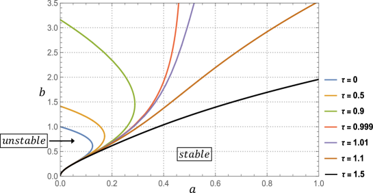
Figure 3: $\tau$-dependence of the bifurcation curves, eq.(14).

(2) Lengyel-Epstein model[13, 16]:

$$\frac{dx}{dt}=a-x-\frac{4xy}{1+x^{2}},~{}\frac{dy}{dt}=bx\left(1-\frac{y}{1+x^{2}}\right),$$ (15)

where $a$ and $b$ are positive bifurcation parameters. In eq.(15), the Hopf bifurcation occurs when $\displaystyle b=\frac{3}{5}a-\frac{25}{a}$. The spiral fixed point of eq. (15) is $\displaystyle\bar{\mathbf{x}}^{(c)}=\left(\frac{a}{5},1+\left(\frac{a}{5}\right)^{2}\right)(=(\bar{x},1+\bar{x}^{2}))$. When $\displaystyle b<\frac{3}{5}a-\frac{25}{a}$, the fixed point $\bar{\mathbf{x}}^{(c)}$ becomes unstable and the limit cycle emerges around $\bar{\mathbf{x}}^{(c)}$. For application of eq.(1) to eq.(15), we divide the right hand sides of eq.(15) into the positive smooth functions $f_{i}$ and $g_{i}$ ($i=1,2$):

$$f_{1}(x,y) = a,~{}g_{1}(x,y)=\frac{4xy}{1+x^{2}}+x,$$

$$f_{2}(x,y) = bx,~{}g_{2}(x,y)=\frac{bxy}{1+x^{2}}.$$ (16)

Then the tropically discretized equation of the Lengyel-Epstein model is obtained as

$$x_{n+1}=\frac{x_{n}+\tau a}{1+\tau(1+\frac{4y_{n}}{1+x_{n}^{2}})},~{}y_{n+1}=\frac{y_{n}+\tau bx_{n}}{1+\tau\frac{bx_{n}}{1+x_{n}^{2}}}.$$ (17)

Here we focus on the type of $\bar{\mathbf{x}}^{(d)}$ in eq.(17). Since $\displaystyle T=\frac{3\bar{x}^{2}-b\bar{x}-5}{1+\bar{x}^{2}},~{}\Delta=\frac{5b\bar{x}}{1+\bar{x}^{2}}(>0),~{}\bar{f}_{1}=a,~{}\bar{f}_{2}=b\bar{x},D_{11}=\frac{3\bar{x}^{2}-5}{1+\bar{x}^{2}},~{}D_{22}=-\frac{b\bar{x}}{1+\bar{x}^{2}}$, we obtain $4\Delta-T^{2}>0$. And we find $\displaystyle A_{nd}=-\frac{32b^{2}\bar{x}^{6}(5+3\bar{x}^{2})}{(1+\bar{x}^{2})^{2}}<0$, $\displaystyle B_{nd}=-\frac{16b\bar{x}^{5}(15+b\bar{x}+7\bar{x}^{2})}{1+\bar{x}^{2}}<0$, and $C_{nd}<0$. Therefore, $P_{nd}(\tau)<0$ and $\bar{\mathbf{x}}^{(d)}$ becomes spiral in eq.(17) for any $\tau>0$. Next, we consider its stability. From eq.(9), the parameters $\alpha(\bar{\mathbf{x}})$ and $\beta(\bar{\mathbf{x}})$ can be calculated as

$$\alpha(\bar{\mathbf{x}}) = \frac{b\bar{x}^{2}}{1+\bar{x}^{2}}(3\bar{x}^{2}-5)=\frac{3}{25}\frac{b\bar{x}^{2}}{1+\bar{x}^{2}}\left(a^{2}-\frac{125}{3}\right),$$

$$\beta(\bar{\mathbf{x}}) = 3\bar{x}^{3}-b\bar{x}^{2}-5\bar{x}$$ (18)

$$= -\bar{x}^{2}\left\{b-\frac{3}{5a}\left(a^{2}-\frac{125}{3}\right)\right\}.$$

If $\displaystyle\alpha(\bar{\mathbf{x}})<0$, or $\displaystyle a^{2}-\frac{125}{3}<0$, then $\beta(\bar{\mathbf{x}})<0$ always holds from eq.(18) and $\bar{\mathbf{x}}^{(d)}$ is stable in eq.(17) based on [St-2]. If $\displaystyle\alpha(\bar{\mathbf{x}})>0$, it is found from [St-1] that $\bar{\mathbf{x}}^{(d)}$ is stable for $0<\tau<\gamma$ and unstable for $\tau>\gamma$, where $\gamma=\displaystyle-\frac{(25+a^{2})(3a^{2}-5ab-125)}{5ab(3a^{2}-125)}$. When $3a^{2}-5ab-125<0$, $\gamma$ becomes positive. Therefore, the Neimark-Sacker bifurcation surface is given as $\tau=\gamma$, namely

$$\tau=-\frac{(25+a^{2})(3a^{2}-5ab-125)}{5ab(3a^{2}-125)}.$$ (19)

Figure 4 shows the projection of the bifurcation surface, eq.(19), on the $ab$-plane. The Neimark-Sacker bifurcation surface exists in the region where $\displaystyle a>5\sqrt{\frac{5}{3}}$ and $\displaystyle b>\frac{3}{5}a-\frac{25}{a}$. When $\tau\to 0$, eq.(19) gives $\displaystyle b=\frac{3}{5}a-\frac{25}{a}$, which coincides with the bifurcation line of eq.(15). The region for the unstable fixed point increases as $\tau$ increases, and in the limit of $\tau\to\infty$, the $ab$-plane is divided into the stable and unstable regions by $\displaystyle a=5\sqrt{\frac{5}{3}}$.

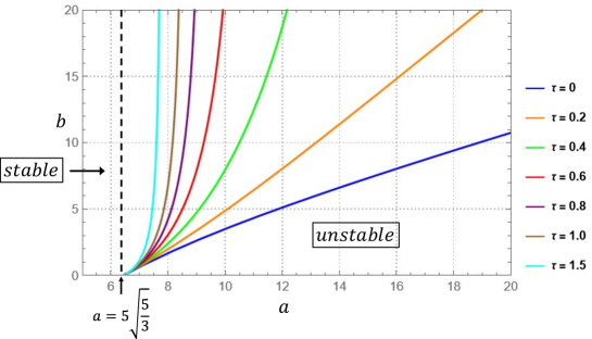
Figure 4: $\tau$-dependence of the bifurcation curves, eq.(19).

Finally, we comment on the relevance of the tropical discretization to the non-standard finite difference scheme [17, 18]. The non-standard finite difference scheme is also known as a positivity-preserving difference scheme and treats the set of differential equations

$$\frac{dx}{dt}=f_{1}(x,y)-xh_{1}(x,y),\frac{dy}{dt}=f_{2}(x,y)-yh_{2}(x,y),$$ (20)

where $f_{i},h_{i}$ are positive smooth functions ($i=1,2$). Their discretized equations are given as

$$x_{n+1} = \frac{x_{n}+\tau f_{1}(x_{n},y_{n})}{1+\tau h_{1}(x_{n},y_{n})},$$

$$y_{n+1} = \frac{x_{n}+\tau f_{2}(x_{n+1},y_{n})}{1+\tau h_{2}(x_{n+1},y_{n})}.$$ (21)

Comparing eq.(21) with eq.(2), we find $x$ in the functions $f_{2}(x,y)$ and $h_{2}(x,y)$ becomes $x_{n+1}$ instead of $x_{n}$. Then the types and stability of the fixed points for eq.(21) are consider to have different properties from the present ones. The dynamical properties of eq.(21) have been already discussed in the previous study[18], but its relationship to the present results is not clear and will be the subject of future work.

4 Conclusion

Relationship of the dynamical properties in the vicinity of fixed points between two-dimensional continuous dynamical systems and their tropically discretized ones has been studied with the aid of the linear stability analysis. The conditions under which the dynamical structures of the original continuous dynamical systems are retained are given by the signs of $\Delta$, $P_{sd}(\tau)$, and $P_{nd}(\tau)$. Moreover, we identify stability of the fixed points in the discrete dynamical system as the conditions for $\tau$. Our general results are successfully applicable to the Sel’kov model and the Lengyel-Epstein model. Especially in the case of the Sel’kov model, our present analytical results are consistent with our previous numerical ones.

Acknowledgments

The authors are grateful to Prof. D. Takahashi, Prof. T. Yamamoto, and Prof. Emeritus A. Kitada at Waseda University, Associate Prof. K. Matsuya at Musashino University, Prof. M. Murata at Tokyo University of Agriculture and Technology for useful comments and encouragements. This work was supported by JSPS KAKENHI Grant Numbers 22K13963 and 22K03442.

References

- [1] M. Murata, Tropical discretization: ultradiscrete Fisher–KPP equation and ultradiscrete Allen–Cahn equation, J. Difference. Equ. Appl., 19 (2013), 1008–1021.
- [2] K. Matsuya and M. Murata, Spatial pattern of discrete and ultradiscrete Gray–Scott model, Discrete Contin. Dyn. Syst. B., 20 (2015), 173–187.
- [3] S. Ohmori and Y. Yamazaki, Cellular automata for spatiotemporal pattern formation from reaction–diffusion partial differential equations, J. Phys. Soc. Jpn., 85 (2016), 045001.
- [4] A. S. Carstea, J. Satsuma, R. Willox and B. Grammaticos, Continuous, discrete and ultradiscrete models of an inflammatory response, Physica A 364 (2006), 276–286.
- [5] R. Willox, A. Ramani, J. Satsuma, and B. Grammaticos, From limit cycles to periodic orbits through ultradiscretisation, Physica A 385 (2007), 473–486.
- [6] S. Gibo and H. Ito, Discrete and ultradiscrete models for biological rhythms comprising a simple negative feedback loop, J. Theor. Biol., 378 (2015), 89–95.
- [7] T. Tokihiro, D. Takahashi, J. Matsukidaira, and J. Satsuma, From soliton equations to integrable cellular automata through a limiting procedure, Phys. Rev. Lett. 76 (1996), 3247-3250.
- [8] S. Ohmori and Y. Yamazaki, Ultradiscrete bifurcations for one dimensional dynamical systems, J. Math. Phys., 61 (2020), 122702.
- [9] S. Ohmori and Y. Yamazaki, Relation of stability and bifurcation properties between continuous and ultradiscrete dynamical systems via discretization with positivity: one dimensional cases, J. Math. Phys., 64 (2023), 042704.
- [10] Y. Yamazaki and S. Ohmori, Periodicity of limit cycles in a max–plus dynamical system, J. Phys. Soc. Jpn., 90 (2021), 103001.
- [11] S. Ohmori and Y. Yamazaki, Dynamical properties of max–plus equations obtained from tropically discretized Sel’kov model, arXiv:2107.02435v1 [nlin.CD].
- [12] S. Ohmori and Y. Yamazaki, Poincaré map approach to limit cycles of a simplified ultradiscrete Sel’kov model, JSIAM Letters, 14 (2022) 127–130.
- [13] S. H. Strogatz, Nonlinear Dynamics and Chaos: With Applications to Physics, Biology, Chemistry, and Engineering, 2nd edn., Westview Press, Cambridge, 2015.
- [14] O. Galor, Discrete Dynamical Systems, Springer, New York, 2010.
- [15] E. E. Sel’kov, Self–oscillations in glycolysis, European J. Biochem., 4 (1968), 79–86.
- [16] I. Lengyel and I. R. Epstein, Science, 251 (1991), 650–652.
- [17] R. E. Mickens, Nonstandard finite difference models of differential equations, World Scientific, Singapore, 1994.
- [18] M. E. Alexander and S. M. Moghadas, shift in Hopf bifurcations for a class of nonstandard numerical schemes, Electron. J. Differ. Equ. Conf. 12 2005, 9–19.