Differentiable programming tensor networks for Kitaev magnets

Abstract

We present a general computational framework to investigate ground state properties of quantum spin models on infinite two-dimensional lattices using automatic differentiation-based gradient optimization of infinite projected entangled-pair states. The approach exploits the variational uniform matrix product states to contract infinite tensor networks with unit-cell structure and incorporates automatic differentiation to optimize the local tensors. We applied this framework to the Kitaev-type model, which involves complex interactions and competing ground states. To evaluate the accuracy of this method, we compared the results with exact solutions for the Kitaev model and found that it has a better agreement for various observables compared to previous tensor network calculations based on imaginary-time projection. Additionally, by finding out the ground state with lower variational energy compared to previous studies, we provided convincing evidence for the existence of nematic paramagnetic phases and 18-site configuration in the phase diagram of the $K$-$\Gamma$ model. Furthermore, in the case of the realistic $K$-$J$-$\Gamma$-$\Gamma^{\prime}$ model for the Kitaev material $\alpha$-RuCl₃, we discovered a non-colinear zigzag ground state. Lastly, we also find that the strength of the critical out-of-plane magnetic field that suppresses such a zigzag state has a lower transition field value than the previous finite-cylinder calculations. The framework is versatile and will be useful for a quick scan of phase diagrams for a broad class of quantum spin models.

I Introduction

The Kitaev model is a prominent example of frustrated magnets, which consists of anisotropic nearest neighbor Ising interactions with three different types of bonds on a honeycomb lattice. The model has an exact solution for its ground state, which hosts a novel phase called quantum spin liquid (QSL) [1]. Moreover, with the proposal of the existence of Kitaev interaction in real materials [2], Kitaev materials like $\alpha$-RuCl₃ have been intensively studied [3, 4, 5, 6, 7]. A bunch of spin models like the $K$-$\Gamma$ model and the $K$-$J$-$\Gamma$-$\Gamma^{\prime}$ model with various couplings were proposed and there was no consensus about which one could fully describe the low energy properties of real materials [3, 4, 8, 9, 10, 11, 12, 13, 14]. There are two major difficulties in the numerical studies of these spin models in the thermodynamic limit. One is that these models are highly frustrated, which causes sign problem in quantum Monte Carlo methods. Though one could avoid this problem by using the tensor network algorithms, another issue may arise. In these models, the competition between various interactions can lead to the formation of magnetic orders with large unit cells. However, dealing with such situations is not easy because of the realistically limited representation capability of one-dimensional (1D) tensor networks, such as the density matrix renormalization group (DMRG) algorithm. While the DMRG algorithm is capable of mapping a two-dimensional (2D) system to a 1D system, the width of the cylinder that can be studied is limited due to computational complexity [15, 16, 17, 18, 19, 20, 21, 22]. Consequently, an alternative method is urgently required to obtain the ground state of systems with frustration and spin configurations characterized by large unit cells.

To solve 2D lattice models directly in the thermodynamic limit, one can use tensor network wave function ansatz, such as the infinite projected entangled-pair states (iPEPS) [23]. Furthermore, multisite iPEPS with the large unit cell can represent complex large configuration wave functions directly [24, 25, 26, 27, 22]. However, there are still two obstructions in the way of conducting groundstate iPEPS calculations with reduced computational cost and improved accuracy.

One obstruction to reducing computational cost is the contraction of the infinite 2D tensor network with a large unit cell. The problem at hand can be addressed through the utilization of the corner transfer matrix renormalization group [28, 29] (CTMRG) and the variational uniform matrix product states [30, 31, 32] (VUMPS) algorithm. These methods effectively contract the infinite 2D tensor network by incorporating the boundary environments. They differ in two distinct ways. Firstly, there is a discrepancy in the contraction order between CTMRG and VUMPS. Secondly, VUMPS directly addresses the eigenproblem, while CTMRG employs a power method-like iteration. The seamless integration of these two techniques presents an intriguing and promising avenue for capitalizing on their respective advantages.

Their computational cost for large unit cell extensions depends linearly on the size of the unit cell. However, it is barely satisfactory that the large unit cell versions of CTMRG and VUMPS both have some tricky problems. The iterative nature of the CTMRG extension, as described by Ref [33], which resembles that of the power method, may affect its rate of convergence to some extent. Moreover, a general principle for optimal approximate contraction has yet to be established. The extension of VUMPS [34] in the large cell does not suffer a such problem. But the non-hermitian transform matrix emerging in the large unit cell is not very well recognized and handled properly until Ref [35]. What’s more, previous work benchmarks their large unit cell in the 2D classical Ising model with $2\times 2$ unit cell. Whether it works well in quantum systems and larger unit cell is unclear.

The other obstruction is the inadequate optimization of iPEPS towards the ground state. In prior works, the imaginary time evolution (ITE) method, including the simple update [36] or full update method [37, 38], is often employed to update iPEPS. Nonetheless, the ground state iPEPS obtained via these methods is often inaccurate due to the separate update of energy bonds, especially in the case of frustrated systems.

Moreover, the effectiveness of the ITE method is heavily reliant on the initialization of iPEPS, particularly for large unit cells. A general approach to finding an unconventional ordered phase using ITE is laborious and heavily relies on artificial expertise. Specifically, the classical model is simulated first [39], followed by an attempt to identify a similar configuration in the quantum case with the same parameters via numerous meticulously selected initializations of iPEPS for the large unit cell [22, 40].

One can leverage differentiable programming techniques for the gradient-based optimization of iPEPS. This approach has been proven to be powerful in spin systems [41, 42, 43], even in the frustrated Kitaev model [44, 45]. Compared to traditional gradient-based tensor methods [46, 47], automatic differentiation (AD) avoids cumbersome graph summations. We observe that optimization, rather than representation ability, is crucial for obtaining the ground state of Kitaev-type frustrated systems because we can obtain the exact ground state energy and correct observables using much smaller iPEPS with virtual bonds $D$ compared to ITE. In principle, once given a forward algorithm to get observables, such as large unit cell VUMPS in this paper, one can get the backward algorithm immediately in the same order of computation complexity. But in practice, we need to carefully design the backward algorithm to guarantee numerical stability and computational efficiency.

In this paper, we will study the iPEPS tensor network ansatz wave functions with large unit cells and their differentiable programming optimization method for the Kitaev-type model. The primary focus of this study is to enhance the optimization capability of iPEPS within comparable dimensions when compared to alternative methodologies, specifically for large unit cell configurations that remain efficient and without artificial effect.

The organization of this paper is as follows. First, Section II reviews the method of ground state iPEPS simulation in the thermodynamic limit and contraction algorithm of large unit cell VUMPS with its carefully designed automatic differentiation optimization. Then, in Section III we present the application in the Kitaev-type systems with various competing phases. Section IV discusses possible issues for future development.

Our paper is accompanied by a ready-to-use Julia package implementing differentiable large unit cell VUMPS calculations [48, 49].

II Methods

We will present a method for obtaining the ground state wave functions in the thermodynamic limit using iPEPS when given a Hamiltonian. Our approach involves first calculating the energy through the contraction of an infinite-sized tensor network with randomly initialized iPEPS. This contraction is performed using the VUMPS algorithm and its larger unit cell version. Then, we will optimize the energy to obtain the iPEPS ground state through the gradient calculated by AD. In this process, a well-designed VUMPS backward will be introduced.

II.1 iPEPS ansatz

In general, accurately representing the quantum state of a system with $N$ sites and $d$ states on each site requires $d^{N}$ parameters, posing significant challenges for numerical simulations, particularly when $N$ is large. Fortunately, the area law of entanglement [50] suggests that a typical quantum ground state is less entangled than an arbitrary state and can be effectively parameterized by tensor networks [51, 52].

The infinite matrix product state (iMPS) and the iPEPS are effective ansatzes for ground states of 1D and 2D systems in the thermodynamic limit respectively. They consist of local tensors that repeat periodically on infinite lattices. The graphical notation of local tensors is shown in Fig. 1, where $D$ is the virtual bond dimension and the corresponding bonds are contracted, $d$ is the bond dimension of physical legs.

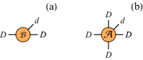
Figure 1: The graphical notation of local tensors. In this notation, each solid shape, such as the above circle, represents a tensor, and each leg (or bond) of it represents an index of the tensor.

Consider a 2D translational invariant system with one site in the unit cell on a square lattice, its ground state can be parameterized by the following iPEPS:

$$|\Psi(\mathcal{A})\rangle= \sum_{\left\{S_{r}\right\}}\operatorname{Tr}\prod_{\mathbf{r}}\mathcal{A}^{S_{r}}[\mathbf{r}]\left|\left\{S_{r}\right\}\right\rangle$$

$$=$$

where $\mathcal{A}^{S_{r}}[\mathbf{r}]$ are the local tensors of rank five, with four virtual bonds and one physical bond. $\left|\left\{S_{r}\right\}\right\rangle=\left|S_{\mathbf{r}_{1}},S_{\mathbf{r}_{2}},\ldots,S_{\mathbf{r}_{\mathbf{N}}}\right\rangle$ is a many-basis state and $\mathbf{r}_{i}$ label different lattice sites. $\mathrm{Tr}[\dots]$ symbolizes the contraction of all virtual bonds.

The energy expectation value is calculated by the following equation:

$$E(\mathcal{A})= \langle\Psi(\bar{\mathcal{A}})|H|\Psi(\mathcal{A})\rangle/\langle\Psi(\bar{\mathcal{A}})\mid\Psi(\mathcal{A})\rangle$$ (1)

$$=$$

where $\bar{\mathcal{A}}$ denotes the conjugate of tensor $\mathcal{A}$ and represents the Hamiltonian tensor that consists of nearest neighbor interaction terms.

To contract the infinite tensor networks as shown in Eq. 1, we firstly contract vertical physical legs and transform the double-layer tensor network with virtual bond dimension $D$ into a single-layer tensor network whose virtual bond dimension is $D^{2}$. For example, the denominator in Eq. 1 becomes

$$\langle\Psi(\bar{\mathcal{A}})\mid\Psi(\mathcal{A})\rangle=\leavevmode\hbox{$\vbox{\hbox{\resizebox{}{}{{\leavevmode\hbox{\set@color{}}}}}}$}$$ (2)

with $M$ being the contraction of $\mathcal{A}$ and $\bar{\mathcal{A}}$:

(3)

where $\bigotimes$ denotes the outer product operation that merges two virtual bonds into one.

Then we introduce the effective boundary environment , which is an approximation of the 2D infinite tensor networks surrounding the local tensor in the center. And  Eq. 1 can be approximated as:

$$E=\leavevmode\hbox{$\vbox{\hbox{\resizebox{}{}{{\leavevmode\hbox{\set@color{}}}}}}$}/\leavevmode\hbox{$\vbox{\hbox{\resizebox{}{}{{\leavevmode\hbox{\set@color{}}}}}}$}$$ (4)

where the contraction of $\mathcal{A}$ tensors and the Hamiltonian tensor is denoted by $MEM$.

Finding the optimal effective boundary environment in Eq. 4 in the key issue in current studies[35]. On the basic intuition of the power method, this would be equivalent to finding the dominant eigenvectors of transfer matrices. To be specific, if we define an infinite one-dimensional row transfer matrix $T$:

and repeatedly apply it on the upper boundary iMPS until convergence, we would get the following fixed-point equation:

(5)

where $\lambda_{u}$ is the largest eigenvalue of $T$. The unpper boundary iMPS is composed of cell tensor $A_{u}$ with virtual bond dimension $\chi$:

(6)

Similarly, one can find the lower-boundary environment iMPS:

(7)

with $A_{d}$ being the cell tensor and $\lambda_{d}$ is the corresponding dominant eigenvalue.

Accordingly, one would be able to contract the 2D infinite tensor network, Eq. 2 for example, row by row and transform it to a one-dimensional infinite tensor network with three rows:

where $N$ denotes the number of rows applied.

This infinite tensor network could also be contracted easily in the same way as discussed before by defining a column transfer matrix , and finding its left and right dominant eigenvectors. The whole 2D infinite tensor network is therefore contracted as:

As a result, the effective boundary environment in Eq. 4 can be written as:

(8)

where $\Lambda$ is an unimportant coefficient consisting of the multiplication of dominant eigenvalues and it would be canceled in the numerator and the denominator of Eq. 4.

II.2 Tensor network contraction: VUMPS

Apart from power iterations, more sophisticated techniques have been developed for determining the effective boundary environment, as demonstrated in Refs. [53, 33, 31]. Among these methods, VUMPS algorithm which iterates fixed-point functions based on the variational principle has attracted much attention due to its high efficiency and extensibility [30, 31, 32]. In this section, we will first introduce VUMPS method that is applicable in the case where the transfer matrix is hermitian. Then discuss its extension to the non-hermitian case. Last, talking about its implementation in more general cases where there is more than one lattice site in a unit cell.

II.2.1 Hermitian VUMPS

Inspired by the DMRG method, the VUMPS algorithm [30] was initially developed to find the ground states of 1D systems. Later, taking advantage of the canonical form and fixed-point functions, this approach was adapted to contract the infinite two-dimensional square lattice tensor networks with hermitian transfer matrices [54]. We will present this algorithm as a prelude, a reader who is familiar with it could move to the next subsection.

Before anything else, let’s first discuss the hermiticity of the transfer matrix. A direct result of a hermitian transfer matrix is that the lower environment is the complex conjugate of the upper environment, which means $A_{d}=\bar{A}_{u}$. This means only one side environment is required and we would see that this also be the key to reformulating the dominant eigenvalue problem to a variational optimization problem. This hermiticity is closely related to the symmetries of physical systems, especially the special reflection that makes:

(9)

This defines the Hermitian adjoint of the matrix product operator in the physical bond.

Another crucial concept is the canonical form of iMPS. For a given tensor $A$, an iMPS is uniquely defined, but the converse is not true. This can be seen from the fact that a local gauge transformation:

leaves the iMPS invariant. Therefore, one can always choose a preferable gauge and the canonical representation is the most commonly used. In this representation, the left-orthonormal tensor $A_{L}$ and the right-orthonormal tensor $A_{R}$ obey the following conditions:

(10)

Suppose the gauge transform between $A_{L}$ and $A_{R}$ is implemented by tensor $C$, center-site tensor $A_{C}$ can thus be defiend:

(11)

Consequently, the canonical form of an iMPS has the following form:

with one $A_{C}$ tensor in the middle and an infinite number of $A_{L}$ and $A_{R}$ tensors on the left and right side of it respectively. The tensor network contraction could be simplified when using canonical representation, and we are going to use it from now on. For more information, please check Ref [54] for details about getting the canonical form and  [48] for code implementation.

It’s time to present the VUMPS algorithm. Just to reiterate, our goal is to find the maximum eigenvalue of the following eigenvalue equation:

$$T|\psi(A)\rangle=\lambda_{\mathrm{row}}|\psi(A)\rangle$$ (12)

or graphacally Eq. 5 and Eq. 7, where $|\psi(A)\rangle$ is the boundary iMPS composed of $A$ tensor. In the case that the transfer matrix ($T$) is hermitian, the variational principle applies and finding the maximum eigenvalue is equivalent to solving:

$$A=\underset{A}{\arg\min}\left(-\log\frac{\langle\psi(\bar{A})|T|\psi(A)\rangle}{\langle\psi(\bar{A})|\psi(A)\rangle}\right)$$ (13)

Instead of the gradient-based optimization method, an iteration method of updating the fixed-point function at zero gradients of Eq. 13 until convergence is used in the VUMPS algorithm, which is proved to be more efficient. When using the canonical representation, the fixed point function can be simplified as:

(14)

where $\lambda_{A_{c}}$ is the corresponding dominant eigenvalue. Apply to the above equation, and let $\lambda_{L}$ be the largest eigenvalue of transfer matrix when applying it to the left environment, we can get another fixed point function:

(15)

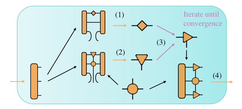
Figure 2: Hermitian VUMPS steps: black arrows are tensor contraction, orange arrows are dominant eigensolvers, and purple arrows are QR decomposition. (1)(2)(4) get dominant eigenvector $A_{C}$,$C$ and $L$,$R$ by their tensor contraction mapping. (3) QR decomposition of $A_{C}$ and $C$ to get $A_{L}$ as Eq. 16

One can use an iterative dominant eigensolver, such as Arnoldi[55], to solve these eigenvalue problems.

The iteration process is shown in Fig. 2. We start by randomly initiating a iMPS local tensor and find its left/right environment $L/R$ in the canonical representation and then go through steps $L,R\rightarrow A_{C},C\rightarrow A_{L},A_{R}$ until convergence. It should be stressed here that  Eq. 11 is not applied in the step $A_{C},C\rightarrow A_{L},A_{R}$, because $C$ may become singular when its dimension is high and this may cause instability in practical calculations of $A_{L}=A_{C}\cdot C^{-1}$. Instead, we apply the QR decomposition of $A_{C}$ and $C$, and get the inversion from the transpose:

$$A_{L} =A_{C}\cdot C^{-1}$$ (16)

$$=Q_{A_{C}}\cdot R_{A_{C}}\cdot R_{C}^{-1}\cdot Q_{C}^{-1}$$

$$=Q_{A_{C}}\cdot R_{A_{C}}\cdot R_{C}^{-1}\cdot Q_{C}^{\dagger}$$

$$\approx Q_{A_{C}}\cdot Q_{C}^{\dagger}$$

The last approximation has a low error when VUMPS converges. So we can define $\|R_{A_{C}}-R_{C}\|$ as the VUMPS algorithm error. Furthermore, $A_{L}$ automatically meet Eq. 10 canonical gauge condition because $Q_{A_{C}}$ and $Q_{C}$ are hermitian. $A_{R}$ can be solved in the same way.

Finally, the effective boundary environment in Eq. 4 corresponding to a hermitian transfer matrix can be written as:

(17)

II.2.2 Non-hermitian VUMPS

In actual physical models, the hermitian condition of the transfer matrix can not always be fulfilled, especially in the case where there is more than one site in a unit cell [56, 35]. So the VUMPS algorithm must be extended to handle more general situations. Though the variational principle is no longer applied here, one can always use the power method to find dominant eigenvectors [54]. As preparation for more complicated cases where there are multi-site unit cells, we limit ourselves to the single-site unit cell case and assume $T$ is non-hermitian in this section, so the reader could get a better understanding of this method.

When the transfer matrix is non-hermitian, we could not get all environment tensors at once as in the hermitian case. We should follow the procedure in Section II.1 and calculate firstly the environment tensors horizontally and then vertically.

We start by discussing a single power step. Given the upper boundary iMPS with bond dimension $\chi$ at $t$-th step, and applying the transfer matrix $T$ to it, the bond dimension would be increased. Our goal is to find another iMPS with bond dimension $\chi$ to approximate it and the new one would serve as the initial iMPS for the $t+1$-th step. The process is represented by the following equation:

where $\lambda_{r}$ is the ratio. We simplify our notation by removing all letters in the tensor notation without ambiguity for the reason that different tensors are denoted by different shapes as in Eq. 11. And the superscript outside of the parentheses labels the power step.

As a consequence, one should maximize the fidelity between two boundary iMPS $|\psi(A^{t})\rangle$ and $|\psi(A^{t+1})\rangle$ within a power step. That leads to a variational optimization for $A^{t+1}$ [54]:

$$\underset{A^{t+1}}{\arg\max}\left(\log\frac{\langle\psi(\bar{A}^{t+1})|T|\psi(A^{t})\rangle\langle\psi(\bar{A}^{t})|T^{\dagger}|\psi(A^{t+1})\rangle}{\langle\psi(\bar{A}^{t+1})|\psi(A^{t+1})\rangle}\right)$$ (18)

It has similar form with  Eq. 13 but to replace $T\rightarrow T|\psi(A^{t})\rangle\langle\psi(\bar{A}^{t})|T^{\dagger}$. Likewise, the corresponding fixed point function could also be written as:

(19)

(20)

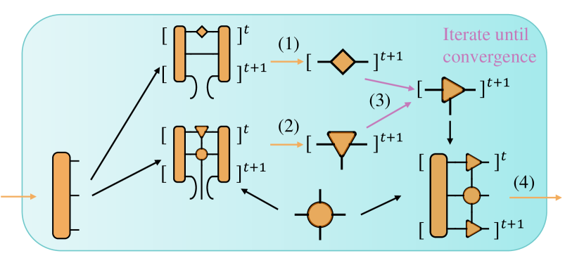
Figure 3: non-hermitian VUMPS steps: different colors and steps (1)(2)(3)(4) meanings are the same as Fig. 2. The difference is that we use superscript for $t$-th iteration in the power method.

It is nothing but to replace $\bar{A}_{L}$ and $\bar{A}_{R}$ in  Eq. 14 and Eq. 15 by their value in the next power step. Following the process in Fig. 3, one can get the optimal upper boundary iMPS.

It is worth noting that, in the case of a non-hermitian transfer matrix, the upper and the lower environments may not exhibit identical characteristics. As a result, it is necessary to repeat the aforementioned calculation to obtain the lower iMPS. This would ultimately result in a computational cost twice as large as that in the hermitian case.

With upper and lower environment tensors in hand, it is easy to contract the infinite three-row tensor and to find the left and right environment tensors. The effective boundary environment in Eq. 4 then be written as:

(21)

II.2.3 Large Unit Cell version of VUMPS

Now we are ready to present the algorithm to deal with general cases with multi-site unit cells. And We developed an easy-used package TeneT.jl specifically for this purpose [48].

Suppose the size of a unit cell of an infinite 2D tensor network on a square lattice is $N_{i}\times N_{j}$, where $N_{i}$ and $N_{j}$ are numbers of lattice sites on each column and row respectively. Take $N_{i}=N_{j}=3$ as an example, the unit cell could be graphically represented as:

(22)

where lattice sites are labeled by their row and column indices. Each row is colored differently for easy distinction. Three transfer matrices $T_{1}$, $T_{2}$ and $T_{3}$ can be defined accordingly. We can see even if the transfer matrix $T_{1}T_{2}T_{3}$ is hermitian, the alternation transfer matrix $T_{2}T_{3}T_{1}$ and $T_{3}T_{1}T_{2}$ are non-hermitian. So we need to find the upper and the lower environment.

Apparently, there are six fixed point equations. Three of them are for upper environments:

(23)

in which the boundary iMPS are defined as:

(24)

While the other three are for lower environments:

(25)

in which the boundary iMPS are:

(26)

The maximum eigenvalue $\lambda_{r}$ is the same in all six equations because of translation invariance while corresponding eigenvectors for different transfer matrices are not equivalent.

If we straightforwardly apply the method discussed in the previous section on these six equations, the computation complexity would be $3\times 3\times 3$ times of that in the single unit cell case, where $3\times 3$ complexity increase comes from the increasing number of parameters within a unit cell and the last $3$ times is a result of three different pair of environments. However, we can use a trick to solve the all upper or lower environments simultaneously and reduce the computation complexity to only $3\times 3$ of that in the single unit cell case. Details are shown below.

It is easy to transform the six equations above into six smaller equations:

(27)

And:

(28)

with $\lambda_{r}=[\lambda_{u}]_{1}[\lambda_{u}]_{2}[\lambda_{u}]_{3}=[\lambda_{d}]_{1}[\lambda_{d}]_{2}[\lambda_{d}]_{3}$, and all $\lambda$s can be different. The price we pay is that these equations are no longer eigenequations and a dominant eigensolver can not be applied anymore. Luckily, an eigenproblem could be reconstructed if we write the group of equations in the following form:

$$\left(\begin{array}[]{lll}&&T_{3}\\ T_{1}&&\\ &T_{2}&\end{array}\right)\left(\begin{array}[]{l}\left[A_{u}\right]_{1,:}\\ \left[A_{u}\right]_{2,:}\\ \left[A_{u}\right]_{3,:}\end{array}\right)=\lambda_{u}\left(\begin{array}[]{l}\left[A_{u}\right]_{1,:}\\ \left[A_{u}\right]_{2,:}\\ \left[A_{u}\right]_{3,:}\end{array}\right)$$ (29)

$$\left(\begin{array}[]{lll}&\tilde{T}_{2}&\\ &&\tilde{T}_{3}\\ \tilde{T}_{1}&&\end{array}\right)\left(\begin{array}[]{l}\left[A_{d}\right]_{1,:}\\ \left[A_{d}\right]_{2,:}\\ \left[A_{d}\right]_{3,:}\end{array}\right)=\lambda_{d}\left(\begin{array}[]{l}\left[A_{d}\right]_{1,:}\\ \left[A_{d}\right]_{2,:}\\ \left[A_{d}\right]_{3,:}\end{array}\right)$$ (30)

where we fix $\lambda_{u}=[\lambda_{u}]_{1}=[\lambda_{u}]_{2}=[\lambda_{u}]_{3}$ and $\lambda_{d}=[\lambda_{d}]_{1}=[\lambda_{d}]_{2}=[\lambda_{d}]_{3}$ for convince. And the colon means the whole row of tensors and the tilde means exchange upper and lower tensor indices.

It is worth mentioning that there is no memory problem even though a large matrix consisting of the transfer matrices is present here since the matrix is not constructed explicitly in practice. We regard Eq. 29 and Eq. 30 as linear maps which are combinations of three fixed point equations as shown above. They can be solved simultaneously by a generic eigensolver such as Arnoldi[55].

Before coming into the power process, let’s explicitly write down the canonical form of the boundary iMPS in large unit cell[34]:

(31)

with:

(32)

where the index of each tensor is carefully labeled.

In this case, applying one-step power means to find:

(33)

where the superscript again labels the $t$-th iteration in the power method and the subscript indicates the equation is for the $i$-th row transfer matrix, $i$ and $i+1$ cyclically permutate between $1$ and $N_{i}=3$. For each function in Eq. 33, the corresponding fixed point equation is:

(34)

(35)

The iteration process for large unit cell cases is presented in Fig. 4

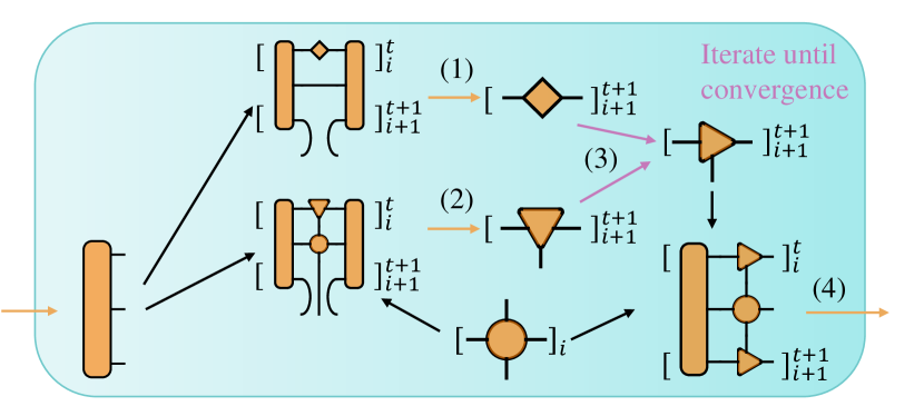
Figure 4: large unit cell VUMPS steps: different colors and steps (1)(2)(3)(4) meanings are the same as Fig. 2. The difference is that we use superscript for $t$-th iteration in the power method and subscript for $i$-th row transfer matrix.

Compared to previous work [34], we enhance the algorithm by iterating the fixed points function Eq. 34 and Eq. 35 with not only row index $i$, but also power index $t$. This is based on the non-Hermitian VUMPS method [54]. In practical applications, our improved iterative approach has demonstrated superior performance compared to the original method.

II.3 Automatic differentiation optimization

The ground state is obtained by optimizing the ground state energy directly using gradient-based optimization on Eq. 1. We calculate its gradient by automatic differentiation, as described in [41], then we optimize the iPEPS using a quasi-Newton L-BFGS algorithm [57]. Compared to numerical differentiation, automatic differentiation can compute derivatives to machine precision and has the same complexity as energy evaluation [58]. Moreover, in comparison with traditional gradient-based tensor methods such as those proposed in [46, 47], automatic differentiation eliminates the need for cumbersome graph summation.

II.3.1 Basics of AD

Automatic differentiation is fundamentally dependent on utilizing the computation graph framework, where nodes within the graph represent data points, and the arrows signify the data flow through computational steps. For example, the simple linear chain computation graph $\theta\rightarrow T_{1}\rightarrow T_{2}\rightarrow\mathcal{L}$ illustrates the process of a vector parameter $\theta$ transforms into a scalar output $\mathcal{L}$. This process is commonly referred to as forward evaluation.

In order to obtain the gradient of $\mathcal{L}$ with respect to $\theta$, the chain rule is utilized as:

$$\frac{\partial\mathcal{L}}{\partial\theta}=\frac{\partial\mathcal{L}}{\partial T_{2}}\frac{\partial T_{2}}{\partial T_{1}}\frac{\partial T_{1}}{\partial\theta}$$ (36)

In most cases where the input dimension is higher than the output dimensions, such as in deep neural networks’ loss function or the free energy in physics, it is more efficient to compute Eq. 36 from left to right. The corresponding computation graph is $\bar{\theta}\leftarrow\bar{T}_{1}\leftarrow\bar{T}_{2}\leftarrow\bar{\mathcal{L}}$. This process involves defining the adjoint variable as $\bar{T}=\partial\mathcal{L}/\partial T$, which denotes the gradient of the final output $\mathcal{L}$ with respect to the variable $T$. The calculation commences from $\bar{\mathcal{L}}=1$ to $\bar{\theta}$, i.e., the gradient, and is conducted through multiple vector-Jacobian product operations that are represented by left arrows. This technique is referred to as reverse-mode automatic differentiation or backward evaluation.

It’s worth noting that computation graphs of iterative tensor network calculations can be quite cumbersome to analyze. Fortunately, modern machine learning frameworks, e.g., PyTorch[59], Jax[60], and Zygote [61], support automatic differentiation on arbitrary complex computations graphs. In principle, once the forward calculation is established, the backward calculation should become readily available. Nonetheless, an optimized efficient forward program may not be differentiable in practice due to in-place memory usage or limitations of the basic library. To solve this difficulty, one can build differentiable primitives by composing many elementary operations like addition, multiplication, and math functions together as a single entity, followed by defining the adjoint of this primitive. Once all primitives in the initial program become differentiable, the whole program becomes differentiable, ensuring that efficiency remains identical to that of the forward computation by careful design.

II.3.2 VUMPS primitives

The computation graph to get iPEPS contraction energy is shown in Fig. 5, and it relies on its subgraph of VUMPS, as shown in Fig. 2. In the VUMPS process, the QR decomposition and dominant eigensolver are non-differentiable directly. Therefore we regard them as primitives and discuss how to obtain their adjoints.

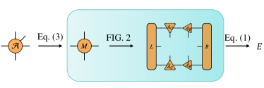
Figure 5: Whole computation graph from iPEPS to energy, where Eq. 3 is constructing $M$ tensor, Fig. 2 is the steps of VUMPS to get environment tensors and Eq. 1 is the 3D contraction for energy

The adjoint of QR decomposition [62] is

$$\bar{\mathcal{M}}=[\bar{Q}+Q\operatorname{Hermitian}(R\bar{R}^{\dagger}-\bar{Q}^{\dagger}Q)](R^{\dagger})^{-1}$$ (37)

where $\operatorname{Hermitian}$ is to replace upper triangular matrix elements with the conjugate of the lower triangular matrix.

The adjoint of the dominant eigensolver is given by paper [63]. The key point is to solve a set of restricted linear equations. The dominant eigenequation is defined as:

$$\bm{l}^{T}\mathcal{M}=\lambda\bm{l}^{T},\quad\mathcal{M}\bm{r}=\lambda\bm{r},\quad\bm{l}^{T}\bm{r}=1$$ (38)

Adjoint of backward is:

$$\bar{\mathcal{M}}=\bar{\lambda}\bm{l}\bm{r}^{T}-\bm{l}\xi_{\bm{l}}^{T}-\xi_{\bm{r}}\bm{r}^{T}$$ (39)

where $\xi_{\bm{l}}$ and $\xi_{\bm{r}}$ are solved by:

$$(\mathcal{M}-\lambda I)\xi_{l} =\left(1-\bm{r}\bm{l}^{T}\right)\bar{\bm{l}}, \bm{l}^{T}\bm{\xi}_{l}=0$$ (40)

$$\left(\mathcal{M}^{T}-\lambda I\right)\xi_{r} =\left(1-\bm{l}\bm{r}^{T}\right)\bar{\bm{r}}, \bm{r}^{T}\xi_{r}=0$$

The above equations should be solved in space that is orthogonal to $\bm{l}$ or $\bm{r}$, but considering $\mathcal{M}-\lambda I$ is not full rank, we only need to solve the equation using an iterative algorithm, such as GMRES [64], with initial guess in this orthogonal space.

In the backward of VUMPS, we only need one side dominant eigenvector, $\bm{l}$ or $\bm{r}$, because we solve the environment separately. So Eq. 39 can be simplified. Firstly, suppose that only $\bm{l}$ is used, $\bar{\lambda}=0$, $\bar{\bm{r}}=0$, and the calculation result is gauge invariant, so [63]

$$\bm{l}^{T}\bar{\bm{l}}=\bm{r}^{T}\bar{\bm{r}}=0$$ (41)

Eq. 40 can be simplified as:

$$(\mathcal{M}-\lambda I)\bm{\xi}_{l} =\bar{\bm{l}}, \bm{l}^{T}\bm{\xi}_{l}=0$$ (42)

$$\left(\mathcal{M}^{T}-\lambda I\right)\bm{\xi}_{r} =0, \bm{r}^{T}\bm{\xi}_{r}=0$$

Assuming $\xi_{r}\neq 0$, $\xi_{r}$ must be a left eigenvector of $\mathcal{M}$, which conflicts with $\bm{r}^{T}\xi_{r}=0$, so $\xi_{r}=0$. Finally, we get adjoint of left dominant eigensolver only with forward of $\bm{l}$:

$$\bar{\mathcal{M}}=-\bm{l}\bm{\xi}_{\bm{l}}^{T}$$ (43)

Similarly, we can get adjoint of the right dominant eigensolver only with forward of $\bm{r}$:

$$\bar{\mathcal{M}}=-\bm{\xi}_{\bm{r}}\bm{r}^{T}$$ (44)

II.3.3 Technical comments

To minimize computational expenses, it is advisable to refrain from constructing the adjoint $\bar{\mathcal{M}}$ tensor for the backward of dominant eigensolver, just as we should avoid constructing $\mathcal{M}$ in the forward. Instead, we can directly construct the adjoint of these two steps, which is the contraction of $\mathcal{M}$ and the dominant eigensolver.

Specifically, when to get the VUMPS environment, we do not construct $\mathcal{M}$ directly. As an illustration, to obtain $L$, the six-rank tensor $\mathcal{M}$, represented by , is subject to contraction by $A_{L}^{u}$, $M$, and $A_{R}^{d}$, resulting in significant memory consumption. Instead, we can define a linear map of this eigenequation, i.e., contract $L$, $A_{L}^{u}$, $M$, $A_{L}^{d}$ in sequence, then solve dominant eigenequation by an iterative method like Krylov subspace method [55, 65, 66]. Performing this linear mapping with an optimal contraction order will result in a four-rank tensor and decrease memory usage.

(45)

Similarly, we do not get $\bar{\mathcal{M}}$ directly in the backward propagation. We get $\bar{M},\bar{A}_{L}^{u},\bar{A}_{L}^{d}$ according to calculation graph $M,A_{L}^{u},A_{L}^{d}\longrightarrow\mathcal{M}\longrightarrow L$. Specifically, solve $\bm{\xi}_{l}$ by the Krylov method using first equation of Eq. 42, then use the contract graph below to get $\bar{A}_{L}^{u},\bar{M},\bar{A}_{L}^{d}$:

(46)

Finally, to ensure the stability and efficiency of backward, there are some crucial tricks:

• The adjoint of QR decomposition include calculation inversion of a matrix, and mix gauge inversion $C^{-1}$ of VUMPS is singular, which means $\det(C)\approx 0$. We solve linear equations by adding a small number($10^{-12}$) to the diagonal of $C$ rather than calculating inversion. This trick can stabilize the calculation at the cost of introducing a small error in the gradient, which has very little effect on the final result experimentally.

• Caused by singularity above, linear equation Eq. 42 is not stable because $\bar{\bm{l}}$ is not orthogonal to $\bm{l}$. So, We should subtract part of $\bar{\bm{l}}$ which is not orthogonal to $\bm{l}$.

• We keep saving and loading the VUMPS environment in the process of optimization for two reasons. One is that inspired by annealing, the iPEPS in two successive steps are only slightly different, and so do the environment tensors. Therefore, loading environment tensors from the previous step as initiation will make the algorithm converge faster. The other is that with fewer forward steps, the gradient explosion is avoided and saves memory usage in the backward process.

• To address the largest memory usage issue arising from the last energy contraction, we employ checkpointing.

III Applications

As a first application of the developed method, we consider the $K$-$J$-$\Gamma$-$\Gamma^{\prime}$ [67, 4, 68] Hamiltonian,

$$\hat{H}= \sum_{\left\langle i,j\right\rangle_{\gamma}}KS_{i}^{\gamma}S_{j}^{\gamma}+J\mathbf{S}_{i}\cdot\mathbf{S}_{j}+\Gamma\left(S_{i}^{\alpha}S_{j}^{\beta}+S_{i}^{\beta}S_{j}^{\alpha}\right)$$ (47)

$$+\Gamma^{\prime}\left(S_{i}^{\alpha}S_{j}^{\gamma}+S_{i}^{\gamma}S_{j}^{\alpha}+S_{i}^{\beta}S_{j}^{\gamma}+S_{i}^{\gamma}S_{j}^{\beta}\right)$$

where $\mathbf{S}_{i}=\{S_{i}^{x},S_{i}^{y},S_{i}^{z}\}$ are the pseudo spin-1/2 operators at site $i$, and $\left\langle i,j\right\rangle_{\gamma}$ denotes the nearest-neighbor pair on the $\gamma$ bond, with $\{\alpha,\beta,\gamma\}$ being $\{x,y,z\}$ under a cyclic permutation. $K$ is the Kitaev coupling, $J$ is the Heisenberg term, $\Gamma$ and $\Gamma^{\prime}$ the off-diagonal couplings.

The Hamiltonian Eq. 47, containing additional terms to the pure Kitaev interaction, is can be used to describe realistic materials such as iridium oxides and $\mathrm{\alpha}$-$\mathrm{RuCl_{3}}$. For example, there is a Heisenberg term $J$ caused by $5d-5d$ superexchange interaction. Moreover, there are $\Gamma$ and $\Gamma^{\prime}$ terms which are superexchange interactions with reduced symmetry due to spin-orbit couplings and lattice distortions in the materials.

The $K$-$J$-$\Gamma$-$\Gamma^{\prime}$ Hamiltonian exhibits a rich phase diagram consisting of ferromagnetic (FM), antiferromagnetic (Néel), zigzag (ZZ), stripy phases [24], as well as more complex phases with 6-site, 18-site unit cells [22, 40]. Our method developed above is ideally suitable to investigate such a problem.

First of all, we group two sites in the unit cell of the honeycomb lattice so we will still deal with iPEPS defined on a square lattice with physical bond dimension $d=2^{2}$, as shown in  Fig. 6(a). Similarly, when considering complex spin-ordered phases, one could similarly group several unit cells to represent a large magnetic unit cell, for example, the black box in Fig. 6(a) represents a magnetic unit cell that consists of four lattice points. 

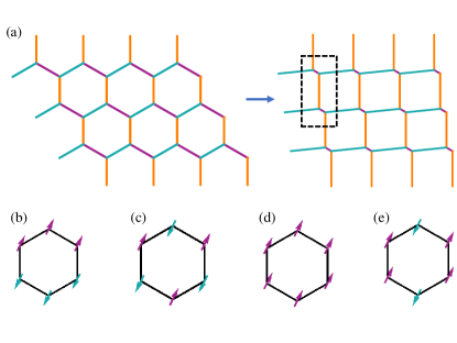
Figure 6: (a) Transformation of the honeycomb lattice to the square lattice by merging two sites in a unit cell of the original honeycomb lattice. $x$-, $y$-, and $z$-bonds are represented by purple, cyan and orange lines, respectively. The dashed black box is $2\times 1$ unit cell and four phases are illustrated: (b) zigzag, (c) Néel, (d) ferromagnetic and (e) stripy phase

III.1 Pure Kitaev model

We start with benchmark calculations of the pure Kitaev model with only $K=-1$ and no other terms. The ground state is exactly solvable [1], and is shown to be a gapless quantum spin liquid without magnetic order. On the other hand, numerical simulations of the Kitaev spin model is nevertheless rather challenging due to high degrees of spin frustrations.

Fig. 7(a) shows that with $D=5$ ($\chi=120$) one can obtain a variational energy $E=-0.196805$ which is in fourth decimal precision agreement with the exact result $-0.19682$. The variational energy is significantly lower than the previous imaginary-time projection-based optimization (full update) up to $D=7$ ($\chi=60$) [24] and comparable to the carefully constructed iPEPS $-0.19681$ with $D=8$ [70]. More importantly, as shown in Fig. 7(b), the variational optimization gives essentially zero magnetization (as small as $10^{-4}$). Also shown in the figures are the unpublished results [44] by differentiating through a CTMRG contraction, which is similar to the recent result [71]. These benchmarks show that even with moderate bond dimensions, one can still obtain highly accurate results on the pure Kitaev model with a more thorough optimization.

The dominant computational complexity of the VUMPS method is equivalent to CTMRG. The computational complexity can be expressed as $\mathcal{O}(D^{6}\chi^{3})$. We performed simulations using an NVIDIA A100-40G GPU. For a pure Kitaev model, it took approximately 4 hours at $D/\chi=4/80$ and 17 hours at $D/\chi=5/120$.

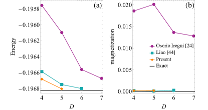
Figure 7: The groundstate energy and magnetization of the pure Kitaev model ($K=-1$) versus $D$. We obtained more accurate results than the ITE and achieved results comparable to CTMRG.

What is noteworthy is that the AD method uses smaller $D$ but larger $\chi$ than ITE to get lower energy. This exactly evidences that the optimization ability of AD is better than ITE and the key point to solving the Kitaev model is optimization ability rather than representation ability. It means representation ability, i.e. the amount of entanglement, of small $D$ is enough to carry the complexity of the Kitaev ground state and large boundary environment bond dimension $\chi$ is needed. The reason why we need larger $\chi$ is that our groundstate iPEPS at the same $D$ is more complex (thus supposed to be highly entangled) than ITE, so we need environments with larger $\chi$, thus more entanglement, to conduct an accurate contraction. To demonstrate this, we examine the convergence of both the energy and the correlation length as a function of the bond dimension $\chi$ in Appendix A. Based on the above results, we find the optimization ability of AD brings iPEPS to an unattainable place for ITE. At the same time, the contraction ability is also crucial and we also overcome this with AD by a sense of annealing as mentioned in Sec. II.3.3.

III.2 Kitaev-$\Gamma$ model

We consider the $K$-$\Gamma$ model with ferromagnetic Kitaev interaction which was proposed to capture the essence of the spin couplings in realistic material RuCl₃ [8, 9]. It was found that there are nematic paramagnetic (NP) and magnetically ordered phases with 18-site unit cells [22, 40] in addition to the Kitaev spin liquid phase (KSL) in the $K$-$\Gamma$ model.

First, we found that the KSL phase survives at $\Gamma=0.03$. Similar to the comparison on the pure Kitaev model in Section III.1, we obtain exact zero magnetization with and lower energy compared to previous iPEPS studies with imaginary-time projection optimization [22].

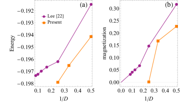
Figure 8: The groundstate energy and magnetization of the $K$-$\Gamma$ model at $\Gamma=0.03$. We obtain lower energy and zero magnetization directly compared to [22].

At $\Gamma=0.095$, the previous study was not conclusive on whether the model shows nematic paramagnetic or ferromagnetic order [22]. Our calculations suggest that the ground state is nematic paramagnetic with anisotropic bond energies, and the results are independent of initialization. Figure 9(a) shows that we’ve obtained much lower variational energy. Extrapolation Figure 9(b) over the bond dimension shows that the obtained state has zero magnetization but finite bond energy anisotropy. Here we define $\Delta E=\mathrm{std}(E_{x},E_{y},E_{z})$ as the standard deviation of the bond energies.

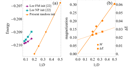
Figure 9: Results of $K$-$\Gamma$ model with $\Gamma=0.095$, where the lower energies compared to previous results in (a) and zero magnetization but non-zero $\Delta E$ in (b) are observed.

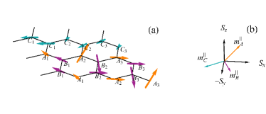
Figure 10: $K$-$\Gamma$ configuration at $\Gamma/|K|=1.0$: the different colors mean $ABC$ components in Section III.2, where these components form a zigzag order in a $2\times 2$ unit cell as shown Fig. 6(b), where they are antiparallel to each other. However, here in panel (a) not all components are antiparallel, and some of them have an angle that deviates from perfect collinearity.

At $\Gamma=1$, we obtain a complex spin-helix order with an 18-site unit cell, shown in Fig. 10(a). Such results confirm previous findings [22, 40] but with lower variational energy per site: -0.3520 at $D=4$ compared with -0.3518 at $D=8$ reported in [40]. Moreover, we obtain the configuration starting from a single randomly initialized calculation rather than repeating hundreds of initial guesses. To minimize the impact of local minima, we also conducted experiments using different unit cell sizes and random initializations to confirm the reliability of our results. When setting the unit cell to be $2\times 2$, we will obtain a zigzag order with higher variational energy compared to the $6\times 3$ configuration shown in Fig. 10(a). On the other hand, when enlarging the unit cell to be 36 sites we still obtain the 18-site order with $10^{-5}$ lower energy per site.

Figure 10(b) show the sublattice magnetization for the three sublattices $\mathbf{m}_{\mu}=\frac{1}{N_{\text{cell }}}\sum_{\text{cells }}\mathbf{S}_{\mu}$ where $\mathbf{m}_{\mu}$ captures the longitudinal components (or rotation axes) of an ensemble of highly structured spin helices.

III.3 $K$-$J$-$\Gamma$-$\Gamma^{\prime}$ model

Finally, we consider the most general form of Hamiltonian Eq. 47. We adopt the model parameters $K=-25\mathrm{meV}$, $\Gamma=0.3|K|$, $\Gamma^{\prime}=-0.02|K|$ and $J=-0.1|K|$ [14], which has been found to fit well most experimental observations in the compound $\alpha$-$\rm{RuCl}_{3}$ [3, 4, 9, 10, 11, 12, 13].

In particular, with such a parameter, DMRG calculations that the ground state shows zigzag magnetic order, which can be suppressed by external magnetic fields.

Under in-plane fields, there is a ZZ to a paramagnetic phase transition, and for an out-of-plane magnetic field there firstly occurs a transition from the ZZ order to the NP phase, before the systems become polarized eventually. To simulate these interesting phases and phase transitions, we introduce magnetic fields to the Hamiltonian by including the term $h\bm{\hat{n}}\cdot\bm{S}$. The direction perpendicular to the plane is represented by $\bm{\hat{n}}=(1,1,1)/\sqrt{3}$ and the direction within the plane is represented by $\bm{\hat{n}}=(1,1,-2)/\sqrt{6}$. $\bm{S}=(S_{x},S_{y},S_{z})$ is spin-1/2 operator and $h$ represents the strength of the field. Reference [14] studied the phase diagram with DMRG and thermal tensor network calculations on a finite cylinder and found it to be consistent with the experimental observations.

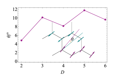
Figure 11: The non-collinear angle $\theta$ of the $K$-$J$-$\Gamma$-$\Gamma^{\prime}$ ground state versus bond dimension $D$ of iPEPS simulations. Inset defines the tilting angle $\theta$.

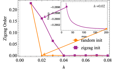
Figure 12: We study the effect of different initializations on the in-plane magnetization process. We compare two cases: random initialization and zigzag initialization, and find that both cases converge to the same final state, but with different optimization steps. Taking $h=0.02$ as an example, when starting from a zigzag state, the system undergoes a transition from zigzag order to a paramagnetic state at the 23rd optimization step, as indicated by the purple arrow in the subfigure energy. This state has the same energy as the one reached by random initialization after 200 optimization steps, as shown by the orange arrow in the subfigure energy.

To start with, we compute the magnetic order under zero field $h=0$. As shown in Fig. 11, indeed we find the spins form a ZZ order. Moreover, we further observe that the magnetic moments are not perfectly anti-parallel, and the conclusion holds for all different bond dimensions in the simulation, where the tilting angle increases with $D$ in Fig. 11. We suppose this non-collinear spin configuration may explain the magnetodielectric effect in the $\alpha$-$\mathrm{RuCl_{3}}$ [72].

In Fig. 12, we show the results under in-plane fields, where the zigzag order parameter vanishes when the field exceeds a certain critical value, revealing a ZZ-PM phase transition. This is consistent with previous model studies [14] and experimental observations [73, 74, 75]. Nevertheless, the critical field values obtained here show some differences from these previous studies. Starting from random iPEPS of bond dimension $D=5$ as initial state, the critical field is found to be $h_{c}/K\simeq 0.02$ that corresponds to 3.5 T (see Fig. 12 orange line), about half the 7-8 T transition field observed in experiments [73, 74, 75] and also in previous DMRG calculations on the same model [14]. Instead, take the ZZ state as the initial state, we find the critical field moves to $h_{c}/K\simeq 0.04$ (about 7 T), and the obtained states are with higher energies (purple line in Fig. 12) in our iPEPS calculations.

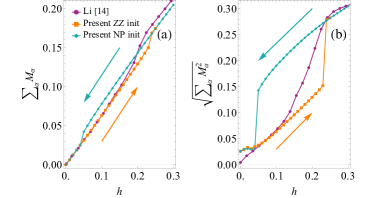
Figure 13: (a) uniform magnetization and (b) a local magnetization from the zigzag and nematic initial phase with $D=5$ iPEPS calculations. The first-order phase transition can be witnessed by a jump in the uniform and local magnetizations. However, the two different schemes, ZZ and NB initializations, produce different transition fields. Note that the local moment $\sqrt{\sum_{\alpha}M_{\alpha}^{2}}$ is finite at the zero field, indicating the presence of ZZ order there.

An out-of-plane field causes a first-order phase transition from the ZZ to NP. We increase the magnetic field from the ZZ phase and reach a critical field of $0.23|K|$ (43 T), consistent with DMRG result [14]. The order parameter jumps sharply at the critical point [see Fig. 13(a)]. However, in the same figure, we also find a quite different transition field when we decrease fields from the NP phase. They even form a hysteresis loop-like shape in Fig. 13(b).

To determine the phase boundary accurately, we use a widely adopted method for first-order phase transition: we initialize the state as either ZZ or NP and look for the crossings of the energy curves. The crossing point converges at $D=5$ (energy difference $<10^{-4}$ Fig. 14), which gives a transition field strength of 0.11$|K|$. This corresponds to 21 T for RuCl₃, which is lower than the DMRG calculations (about 35 T). This suggests that accurate determination of the first-order transition field may be tricky and affected by finite-size effects in DMRG calculations on cylinders of limited widths.

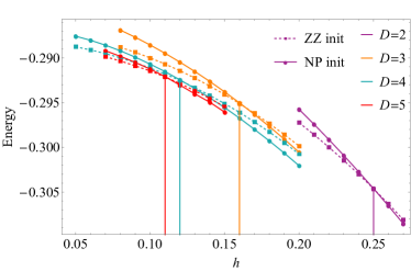
Figure 14: Initialized from ZZ or NP phase, we determine the transition point by the energy cross point. The energy cross between results with different initial states, ZZ and NP, which influence the energy values, and thus the cross points. The crossing points are about to converge for $D=5$ and found to be $h=0.11|K|$.

Overall, the $K$-$J$-$\Gamma$-$\Gamma^{\prime}$ model captures the essential features of the magnetic order and phase transitions observed in $\alpha$-$\mathrm{RuCl_{3}}$. The model provides valuable insights into the behavior of this compound and its response to external magnetic fields, although the exact matching of critical field values between simulations and experiments may still pose challenges due to various factors, including the complexities of experimental fitting and the influence of finite-size/$\chi$ effects in numerical calculations. Further advances in determining the Hamiltonian parameters and experimental phase boundaries are needed to fully confirm these findings.

IV Discussions

We have shown that differentiable programming tensor networks can produce highly accurate results in Kitaev-type frustrated magnet spin systems. The method provides more reliable results compared to previous iPEPS calculations with simple or full update methods. For example, one can obtain a more accurate ground state even with smaller bond dimensions. Moreover, the findings are also less sensitive to the initial state used in the optimization (except for the case near first-order quantum phase transition). Differentiable programming tensor networks are easy to implement but perform excellently. The framework is generic and can be applied to any 2D quantum system with short-range interactions.

We have also performed some calculations with fermionic tensor networks with U(1) symmetry implemented (in either spin or charge channel) and achieved consistent results from the full update calculations. However, the U(1) block structure complicates the use of our AD method in fermionic iPEPS. One limitation arises when dividing the iPEPS tensor, as different block divisions can lead to different ground state energies, necessitating manual selection of block divisions. Another limitation arises as in the VUMPS one is unable to choose block divisions for the environment. This is because VUMPS does not use SVD, which is a crucial step for selecting block divisions in other methods such as CTMRG or TEBD. We plan to address these issues in future work.

V Acknowledgments

We thank Hao Xie, Qi Yang, Han Li, Shou-Shu Gong, Shun-Yao Yu, Hao-Kai Zhang, Qiang Luo, Ke Liu, and Philippe Corboz for the discussion. We thank Juan Osorio Iregui for providing the reference data shown in Fig. 7. This project is supported by the National Key Projects for Research and Development of China Grant. No. 2021YFA1400400 and No. 2022YFA1403900, Strategic Priority Research Program of the Chinese Academy of Sciences under Grant No. XDB30000000, National Natural Science Foundation of China (Grant Nos. T2225018, T2121001, 12222412, 11834014, 11974036), CAS Project for Young Scientists in Basic Research (Grant No. YSBR-057), China Postdoctoral Science Foundation under Grant No. 2021TQ0355, the Special Research Assistant Program of Chinese Academy of Sciences and the Youth Innovation Promotion Association CAS under Grant No. 2021004.

Appendix A The convergence versus the boundary bond dimension

The figure below illustrates the energy and correlation length ($\xi$) as a function of the bond dimension $\chi$ of the boundary environment in the pure Kitaev model simulations. It clearly demonstrates the convergence behavior occurring at approximately $\chi=120$. Although the energy fluctuates by $10^{-5}$, we observe that the correlation length doubles as we increase the bond dimension from $\chi=60$ to $\chi=120$.

The maximum are $D/\chi=4/80,5/120,6/150$ in our optimization simulations and larger $\chi$ to insure the convergence of the observables.

References

- Kitaev [2006] A. Kitaev, Annals of Physics 321, 2 (2006), january Special Issue.
- Jackeli and Khaliullin [2009] G. Jackeli and G. Khaliullin, Phys. Rev. Lett. 102, 017205 (2009).
- Winter et al. [2016] S. M. Winter, Y. Li, H. O. Jeschke, and R. Valentí, Phys. Rev. B 93, 214431 (2016).
- Winter et al. [2017] S. M. Winter, A. A. Tsirlin, M. Daghofer, J. van den Brink, Y. Singh, P. Gegenwart, and R. Valentí, Journal of Physics: Condensed Matter 29, 493002 (2017).
- Hermanns et al. [2018] M. Hermanns, I. Kimchi, and J. Knolle, Annual Review of Condensed Matter Physics 9, 17 (2018), https://doi.org/10.1146/annurev-conmatphys-033117-053934 .
- Takagi et al. [2019] H. Takagi, T. Takayama, G. Jackeli, G. Khaliullin, and S. E. Nagler, Nature Reviews Physics 1, 264 (2019).
- Glamazda et al. [2017] A. Glamazda, P. Lemmens, S.-H. Do, Y. S. Kwon, and K.-Y. Choi, Phys. Rev. B 95, 174429 (2017).
- Wang et al. [2017] W. Wang, Z.-Y. Dong, S.-L. Yu, and J.-X. Li, Phys. Rev. B 96, 115103 (2017).
- Ran et al. [2017] K. Ran, J. Wang, W. Wang, Z.-Y. Dong, X. Ren, S. Bao, S. Li, Z. Ma, Y. Gan, Y. Zhang, J. T. Park, G. Deng, S. Danilkin, S.-L. Yu, J.-X. Li, and J. Wen, Phys. Rev. Lett. 118, 107203 (2017).
- Suzuki and Suga [2019] T. Suzuki and S.-i. Suga, Phys. Rev. B 99, 249902 (2019).
- Wu et al. [2018] L. Wu, A. Little, E. E. Aldape, D. Rees, E. Thewalt, P. Lampen-Kelley, A. Banerjee, C. A. Bridges, J.-Q. Yan, D. Boone, S. Patankar, D. Goldhaber-Gordon, D. Mandrus, S. E. Nagler, E. Altman, and J. Orenstein, Phys. Rev. B 98, 094425 (2018).
- Cookmeyer and Moore [2018] T. Cookmeyer and J. E. Moore, Phys. Rev. B 98, 060412 (2018).
- Sandilands et al. [2016] L. J. Sandilands, Y. Tian, A. A. Reijnders, H.-S. Kim, K. W. Plumb, Y.-J. Kim, H.-Y. Kee, and K. S. Burch, Phys. Rev. B 93, 075144 (2016).
- Li et al. [2021] H. Li, H.-K. Zhang, J. Wang, H.-Q. Wu, Y. Gao, D.-W. Qu, Z.-X. Liu, S.-S. Gong, and W. Li, Nature Communications 12, 1 (2021).
- Jiang et al. [2011] H.-C. Jiang, Z.-C. Gu, X.-L. Qi, and S. Trebst, Phys. Rev. B 83, 245104 (2011).
- Vodola et al. [2015] D. Vodola, L. Lepori, E. Ercolessi, and G. Pupillo, New Journal of Physics 18, 015001 (2015).
- Gergs et al. [2016] N. M. Gergs, L. Fritz, and D. Schuricht, Phys. Rev. B 93, 075129 (2016).
- Gohlke et al. [2017] M. Gohlke, R. Verresen, R. Moessner, and F. Pollmann, Phys. Rev. Lett. 119, 157203 (2017).
- Gohlke et al. [2018a] M. Gohlke, R. Moessner, and F. Pollmann, Phys. Rev. B 98, 014418 (2018a).
- Zhu et al. [2018] Z. Zhu, I. Kimchi, D. N. Sheng, and L. Fu, Phys. Rev. B 97, 241110 (2018).
- Gohlke et al. [2018b] M. Gohlke, G. Wachtel, Y. Yamaji, F. Pollmann, and Y. B. Kim, Phys. Rev. B 97, 075126 (2018b).
- Lee et al. [2020] H.-Y. Lee, R. Kaneko, L. E. Chern, T. Okubo, Y. Yamaji, N. Kawashima, and Y. B. Kim, Nature Communications 11, 1639 (2020).
- Verstraete and Cirac [2004] F. Verstraete and J. I. Cirac, Renormalization algorithms for quantum-many body systems in two and higher dimensions (2004), arXiv:cond-mat/0407066 [cond-mat.str-el] .
- Osorio Iregui et al. [2014] J. Osorio Iregui, P. Corboz, and M. Troyer, Phys. Rev. B 90, 195102 (2014).
- Gotfryd et al. [2017] D. Gotfryd, J. Rusnačko, K. Wohlfeld, G. Jackeli, J. c. v. Chaloupka, and A. M. Oleś, Phys. Rev. B 95, 024426 (2017).
- Chen et al. [2018] J.-Y. Chen, L. Vanderstraeten, S. Capponi, and D. Poilblanc, Phys. Rev. B 98, 184409 (2018).
- Czarnik et al. [2019] P. Czarnik, A. Francuz, and J. Dziarmaga, Phys. Rev. B 100, 165147 (2019).
- Nishino and Okunishi [1997] T. Nishino and K. Okunishi, Journal of the Physical Society of Japan 66, 3040 (1997), https://doi.org/10.1143/JPSJ.66.3040 .
- Orús and Vidal [2009] R. Orús and G. Vidal, Phys. Rev. B 80, 094403 (2009).
- Zauner-Stauber et al. [2018] V. Zauner-Stauber, L. Vanderstraeten, M. T. Fishman, F. Verstraete, and J. Haegeman, Phys. Rev. B 97, 045145 (2018).
- Fishman et al. [2018] M. T. Fishman, L. Vanderstraeten, V. Zauner-Stauber, J. Haegeman, and F. Verstraete, Phys. Rev. B 98, 235148 (2018).
- Vanderstraeten et al. [2019] L. Vanderstraeten, J. Haegeman, and F. Verstraete, SciPost Phys. Lect. Notes , 7 (2019).
- Corboz et al. [2014] P. Corboz, T. M. Rice, and M. Troyer, Phys. Rev. Lett. 113, 046402 (2014).
- Nietner et al. [2020] A. Nietner, B. Vanhecke, F. Verstraete, J. Eisert, and L. Vanderstraeten, Quantum 4, 328 (2020).
- Vanderstraeten et al. [2022] L. Vanderstraeten, L. Burgelman, B. Ponsioen, M. Van Damme, B. Vanhecke, P. Corboz, J. Haegeman, and F. Verstraete, Phys. Rev. B 105, 195140 (2022).
- Jiang et al. [2008] H. C. Jiang, Z. Y. Weng, and T. Xiang, Phys. Rev. Lett. 101, 090603 (2008).
- Corboz et al. [2010] P. Corboz, R. Orús, B. Bauer, and G. Vidal, Phys. Rev. B 81, 165104 (2010).
- Phien et al. [2015] H. N. Phien, J. A. Bengua, H. D. Tuan, P. Corboz, and R. Orús, Phys. Rev. B 92, 035142 (2015).
- Rayyan et al. [2021] A. Rayyan, Q. Luo, and H.-Y. Kee, Phys. Rev. B 104, 094431 (2021).
- Li et al. [2022] J.-W. Li, N. Rao, J. von Delft, L. Pollet, and K. Liu, Tangle of spin double helices in the honeycomb kitaev- model (2022), arXiv:2206.08946 [cond-mat.str-el] .
- Liao et al. [2019] H.-J. Liao, J.-G. Liu, L. Wang, and T. Xiang, Phys. Rev. X 9, 031041 (2019).
- Hasik et al. [2021] J. Hasik, D. Poilblanc, and F. Becca, SciPost Phys. 10, 012 (2021).
- Xi et al. [2021] N. Xi, H. Chen, Z. Y. Xie, and R. Yu, First-order transition between the plaquette valence bond solid and antiferromagnetic phases of the shastry-sutherland model (2021).
- Liao [2019] H.-J. Liao, talk at Tokyo ISSP (2019), https://www.youtube.com/watch?v=Z4kTT6SKtVk Accessed March 28, 2023.
- Hasik et al. [2022] J. Hasik, M. Van Damme, D. Poilblanc, and L. Vanderstraeten, Phys. Rev. Lett. 129, 177201 (2022).
- Corboz [2016] P. Corboz, Phys. Rev. B 94, 035133 (2016).
- Vanderstraeten et al. [2016] L. Vanderstraeten, J. Haegeman, P. Corboz, and F. Verstraete, Phys. Rev. B 94, 155123 (2016).
- Zhang [2022a] X.-Y. Zhang, Vumps julia package, [EB/OL] (2022a), https://github.com/XingyuZhang2018/TeneT.jl Accessed March 28, 2022.
- Zhang [2022b] X.-Y. Zhang, applications in section iii, [EB/OL] (2022b), https://github.com/XingyuZhang2018/AD-Kitaev Accessed March 28, 2022.
- Eisert et al. [2010] J. Eisert, M. Cramer, and M. B. Plenio, Rev. Mod. Phys. 82, 277 (2010).
- Schollwöck [2005] U. Schollwöck, Rev. Mod. Phys. 77, 259 (2005).
- Pérez-García et al. [2007] D. Pérez-García, F. Verstraete, M. M. Wolf, and J. I. Cirac, Quantum Inf. Comput. 7, 401 (2007).
- Corboz et al. [2011] P. Corboz, S. R. White, G. Vidal, and M. Troyer, Phys. Rev. B 84, 041108 (2011).
- Vanhecke et al. [2021a] B. Vanhecke, M. V. Damme, J. Haegeman, L. Vanderstraeten, and F. Verstraete, SciPost Phys. Core 4, 004 (2021a).
- Arnoldi [1951] W. E. Arnoldi, Quarterly of applied mathematics 9, 17 (1951).
- Vanhecke et al. [2021b] B. Vanhecke, J. Colbois, L. Vanderstraeten, F. Verstraete, and F. Mila, Phys. Rev. Res. 3, 013041 (2021b).
- Nocedal and Wright [2006] J. Nocedal and S. Wright, New York (2006).
- Baur and Strassen [1983] W. Baur and V. Strassen, Theoretical Computer Science 22, 317 (1983).
- Paszke et al. [2017] A. Paszke, S. Gross, S. Chintala, G. Chanan, E. Yang, Z. DeVito, Z. Lin, A. Desmaison, L. Antiga, and A. Lerer, Automatic differentiation in pytorch (2017).
- Frostig et al. [2018] R. Frostig, M. J. Johnson, and C. Leary, Systems for Machine Learning 4 (2018).
- Innes [2019] M. Innes, Don’t unroll adjoint: Differentiating ssa-form programs (2019), arXiv:1810.07951 [cs.PL] .
- Seeger et al. [2019] M. Seeger, A. Hetzel, Z. Dai, E. Meissner, and N. D. Lawrence, Auto-differentiating linear algebra (2019), arXiv:1710.08717 [cs.MS] .
- Xie et al. [2020] H. Xie, J.-G. Liu, and L. Wang, Phys. Rev. B 101, 245139 (2020).
- Saad and Schultz [1986] Y. Saad and M. H. Schultz, SIAM Journal on Scientific and Statistical Computing 7, 856 (1986).
- Lehoucq et al. [1998] R. B. Lehoucq, D. C. Sorensen, and C. Yang, ARPACK Users’ Guide (Society for Industrial and Applied Mathematics, University City, Philadelphia, 1998) https://epubs.siam.org/doi/pdf/10.1137/1.9780898719628 .
- Haegeman [2022] J. Haegeman, julia package for krylov space method, [EB/OL] (2022), https://github.com/Jutho/KrylovKit.jl Accessed March 28, 2022.
- Rau et al. [2014] J. G. Rau, E. K.-H. Lee, and H.-Y. Kee, Phys. Rev. Lett. 112, 077204 (2014).
- Chaloupka et al. [2010] J. c. v. Chaloupka, G. Jackeli, and G. Khaliullin, Phys. Rev. Lett. 105, 027204 (2010).
- Note [1] In contrast with brick-wall lattice [24], this transformation merging two sites contains twice the physical bonds but half the number of unit cells. In practice, we find such a scheme is more effective and thus use it in later simulations.
- Lee et al. [2019] H.-Y. Lee, R. Kaneko, T. Okubo, and N. Kawashima, Phys. Rev. Lett. 123, 087203 (2019).
- Lukin and Sotnikov [2023] I. V. Lukin and A. G. Sotnikov, Phys. Rev. B 107, 054424 (2023).
- Aoyama et al. [2017] T. Aoyama, Y. Hasegawa, S. Kimura, T. Kimura, and K. Ohgushi, Phys. Rev. B 95, 245104 (2017).
- Banerjee et al. [2017] A. Banerjee, J. Yan, J. Knolle, C. A. Bridges, M. B. Stone, M. D. Lumsden, D. G. Mandrus, D. A. Tennant, R. Moessner, and S. E. Nagler, Science 356, 1055 (2017).
- Zheng et al. [2017] J. Zheng, K. Ran, T. Li, J. Wang, P. Wang, B. Liu, Z.-X. Liu, B. Normand, J. Wen, and W. Yu, Phys. Rev. Lett. 119, 227208 (2017).
- Modic et al. [2021] K. A. Modic, R. D. McDonald, J. P. C. Ruff, M. D. Bachmann, Y. Lai, J. C. Palmstrom, D. Graf, M. K. Chan, F. F. Balakirev, J. B. Betts, G. S. Boebinger, M. Schmidt, M. J. Lawler, D. A. Sokolov, P. J. W. Moll, B. J. Ramshaw, and A. Shekhter, Nature Physics 17, 240 (2021).