Abstract. A diffused interface model describing the evolution of two conterminous incompressible fluids in a porous medium is discussed. The system consists of the Cahn-Hilliard equation with Flory-Huggins logarithmic potential, coupled via surface tension term with the evolutionary Stokes equation at the pore scale. An evolving diffused interface of finite thickness, depending on the scale parameter $\varepsilon$ separates the fluids. The model is studied in a bounded domain $\Omega$ with a sufficiently smooth boundary $\partial\Omega$ in $\mathbb{R}^{d}$ for $d=2$, $3$. At first, we investigate the existence of the system at the micro-scale and derive the essential a-priori estimates. Then, using the two-scale convergence approach and unfolding operator technique, we obtain the homogenized model for the microscopic one.
 

Keywords: Diffused interface model, Stokes, Cahn-Hilliard, logarithmic potential, porous media flow, existence of solution, Galerkin approximation, homogenization, two-scale convergence, periodic unfolding.
AMS subject classifications: 35K57, 35K91, 35B27, 76M50  

1 Introduction

Multiphase flows appear in many natural, biological and industrial processes such as sediment transport (in rivers), groundwater flows through rocks, oil reservoirs, multiphase flows in channels and porous media. Phase-field approach is a popular tool for modeling and simulating two or multiphase flow problems, cf. [31, 21, 6, 8, 9]. The Cahn-Hilliard system plays an essential role in material science, describing imperative qualitative features of two-phase systems related to phase separation processes, inferring isotropy and constant temperature throughout, cf. [38]. The dynamics of the phase interface between fluids play a central role in rheology and hydrodynamics in the case of fluid mixtures, cf. [33, 12, 20]. In [43], the concept of local thermodynamic equilibrium of a Gibbs interface is discussed to relax the global thermodynamic equilibrium assumption, which extends towards non-equilibrium two-phase systems. In [34], the diffused interface and Cahn-Hilliard formulation of a quasi-compressible binary fluid mixture have been studied by by considering the topological interface changes. Over the last few decades, the coupling of the Navier-Stokes system with the Cahn-Hilliard equations has become a topic of great interest due to its wide range of applications in the industry and engineering. In [21], a fully discrete mixed finite element method for approximating the coupled system is proposed in which, the two sets of equations are coupled through a different phase induced stress term in the Navier–Stokes equations and a fluid-induced transport term in the Cahn–Hilliard equation. In [9], a system of the Navier-Stokes equations coupled with multicomponent Cahn-Hilliard variational inequalities is considered, where the existence of the weak solutions of the model is shown via a fully discrete finite element approximation.

$$\partial_{t}c+\mathbf{u}\cdot\nabla c =\Delta w \text{ in }(0,T)\times\Omega,$$ (1.1a)

$$w =-\Delta c+f(c) \text{ in }(0,T)\times\Omega,$$ (1.1b)

$$\partial_{t}\mathbf{u}-\mu\Delta{\mathbf{u}}+\nabla p =\lambda c\nabla w \text{ in }(0,T)\times\Omega,$$ (1.1c)

$$\nabla\cdot\mathbf{u} =0 \text{ in }(0,T)\times\Omega,$$ (1.1d)

In this paper, we consider the coupled Stokes-Cahn-Hilliard system, see (1.1), for which the detail is provided in section 1.1. The well-posedness of the Cahn-Hilliard system and Stokes equation in single domains have been extensively studied in the literature. In [11, 12], mathematical analysis of the Navier-Stokes-Cahn-Hilliard system for different cases can be captured. In [1], the uniqueness and regularity of the two-phase field model for viscous, incompressible fluid with matched densities have been extensively investigated. In [2], the authors discuss the existence of strong solutions locally in time for a model of a binary mixture of viscous incompressible fluids in a bounded domain. In [3], the existence of weak solutions for a diffuse interface model for the flow of two viscous incompressible Newtonian fluids in a bounded domain by allowing for degenerate mobility has been proven. Recently, in [25], the well-posedness of the Cahn-Hilliard-Hele-Shaw system with singular potential has been studied extensively. In [27], a rigorous study on the uniqueness and regularity of the Navier-Stokes-Cahn-Hilliard system for two and three-dimensional bounded domain was done, which further has been extended to the existence of strong solutions to the Cahn-Hilliard-Darcy system with mass source in [26]. However, the homogenization results are not shown in their work.

Mathematically, using the methods of homogenization, cf. [5, 4, 29, 40, 15, 13, 39], single-phase flow in porous media can be approximated by Darcy’s Law [30]. This equation can be derived from Stokes equations for single-phase flow in the pore part and is parametrized by the hydraulic conductivity. Such techniques have been applied in single porosity materials [29] and dual porosity materials [7]. A derivation of macroscopic Cahn-Hilliard equations for perforated domains is given in [44]. In [45], under the assumptions of periodic flow and a sufficiently large P$\acute{e}$clet number, a basic phase-field model for a mixture of two incompressible fluids in a heterogeneous domain is upscaled via periodic homogenization. In [44, 45], homogenization of the Cahn–Hilliard model in porous media has previously been studied for a case in which the interface thickness is comparable with the characteristic pore size. Subsequently, in [8], the authors considered a phase-field model for two-phase immiscible, incompressible porous media flow with surface tension effects and proved the existence and homogenized the system with bi-quadratic polynomial potential functional under the assumption of periodic flow.

In the present work, we aim to study the existence of solution and homogenization of a diffused interface model, which leads to a system describing the flow of two incompressible Newtonian fluids of the same density and viscosity in porous media where the Stokes-Cahn-Hilliard equations model the problem. Although it is assumed that the fluids are macroscopically immiscible, the model takes a partial mixing on a small length scale measured by a parameter $\varepsilon>0$ into account. Therefore, the sharp classical interface between both fluids is replaced by an interfacial region. In such binary fluids, the phase-field method employs a phase variable or the order parameter $-1\leq c\leq 1$ to track each phase: $c=1$ describes the region occupied by fluid 1, and $c=-1$ denotes the one occupied by fluid 2, while $-1<c<1$ represents the interfacial region. Note that such a process restricts the diffusion process to the interfacial region. To the best knowledge of the authors, this is the first attempt of upscaling the Stokes-Cahn-Hilliard system with logarithmic potential in such periodic domains. We prove the existence of the considered model with singular (1.3) and approximated (3.30) logarithmic potential functional in this work. However, the upscaling of the approximated potential will be regarded in our upcoming work, which is much more crucial to handle mathematically and of great interest.
Plan of the paper. In section 1.1, we present the configuration of a periodic porous medium and the considered binary-fluid model. In section 1.2, the pore scale setting of the model is done, and the model equations are introduced. In section 2, notations, function space and mathematical prerequisites are gathered for the analysis. In section 3, we will prove the existence of the solution of the coupled system. Eventually, in section 4, we obtain the upscaled model of the microscopic problem via two-scale convergence and unfolding operator technique. According to the model, the appropriate initial and boundary conditions will be discussed further in the next section. In Appendix, we report some mathematical tools regarding the analysis and various definitions and results related to homogenization theory.

1.1 Mathematical setting of the model

Let the bulk $\Omega\subset\mathbb{R}^{d}$ ($d=2$ or $3$) be a bounded domain with a sufficiently smooth boundary $\partial\Omega$. To start with, we consider a pore-scale model where the two immiscible fluids occupy two disjoint subdomains of the pore space separated by an interface of thickness $\lambda$ that moves with the fluid flow. The model includes the surface tension effects on the motion of the interface. Several papers, for instance [1, 45, 28, 11, 8], offer to regard the below system of coupled unsteady Stokes-Cahn-Hilliard equations in such case

$$\partial_{t}c+\mathbf{u}\cdot\nabla c =\Delta w \text{ in }(0,T)\times\Omega,$$ (1.2a)

$$w =-\Delta c+f(c) \text{ in }(0,T)\times\Omega,$$ (1.2b)

$$\partial_{t}\mathbf{u}-\mu\Delta{\mathbf{u}}+\nabla p =\lambda c\nabla w \text{ in }(0,T)\times\Omega,$$ (1.2c)

$$\nabla\cdot\mathbf{u} =0 \text{ in }(0,T)\times\Omega,$$ (1.2d)

on the time interval $(0,T)$, $T>0$. The addition of the advection (or transport) term in (1.2a) is quite natural, and the force term (surface tension) is acting only near the interface in (1.2c). In (1.2) $\mathbf{u}$ and $w$ are the unknown velocity and chemical potential, respectively. $\mu$ is the viscosity and $\lambda$ is the interfacial width parameter. Here $c$ represents the microscopic concentration of one of the fluids with values lying in the interval $[-1,1]$ in the considered domain and $(-1,1)$ within the thin diffused interface of uniform width proportional to $\lambda$. The mobility $M(c)$ is taken to be $1$ to avoid a mathematical difficulty, cf. [11]. It is assumed that the densities of both components and the mixture are constant and, for simplicity, equal to $1$. The viscosity of both the fluids is chosen to be a positive constant $\mu$, known as the matched viscosity case in the literature.
The term $f$ is the derivative of $F$, where the function $F$ represents a homogeneous free energy potential functional that penalizes the deviation from the physical constraint, $\absolutevalue{c}\leq 1$. The potential $F$ must have a double-well structure, each depicting the phases of the mixture. In several cases, authors (for eg. [10, 17, 11, 38]), have proposed to consider the thermodynamically relevant potential functionals such as

$$F(s) =\frac{1}{4}(s^{2}-1)^{2} \forall s\in[-1,1],$$

$$F(s) =\frac{\theta_{0}}{2}(1-s^{2})+\frac{\theta}{2}\Big{(}(1-s)\ln{\frac{1-s}{2}}+(1+s)\ln{\frac{1+s}{2}}\Big{)} \forall s\in[-1,1].$$ (1.3)

The latter is known as the physically relevant Flory-Huggins logarithmic potential, which has been used in [1, 11, 25, 27, 26]. However, the domain of the logarithmic potential is an open interval $(0,1)$, so it must be strictly ensured that the value of the calculated solution belongs to this domain; otherwise, the calculation will easily overflow. Therefore, the modified logarithmic potential usually comes into practice: extended form, defined on $(-\infty,\infty)$. In (1.3), $\theta$ and $\theta_{0}$ are constant parameters related to the absolute and critical temperature of the fluid mixture, respectively, which satisfy the physical relation $0<\theta<\theta_{0}$. The condition $0<\theta<\theta_{0}$ ensures that $F$ has a double-well form and that the phase separation can occur. Also, note that the polynomial approximation is reasonable when the quench is shallow, i.e., when the absolute temperature is close to the critical one. In the sequel of our work, we make a few assumptions on the function $F$, which satisfy the above choices. By the mathematical analysis of (1.2) along with (appropriate) initial and boundary conditions, see (1.5), one may find a solution $c$, attaining arbitrary values in $\mathbb{R}$, no matter what type of potential is taken into account. However, we permanently restrict it following its very definition, $\absolutevalue{c}\leq 1$, calling these physical solutions. More precisely, we have

$$c\in L^{\infty}\left((0,\infty)\times\Omega\right)\text{ with }\absolutevalue{c(t,x)}<1\text{ a.e. }(x,t)\in(0,\infty)\times\Omega.$$ (1.4)

The nonlinear term $c\nabla w$ in (1.2c) models the surface tension effects, and advection effect is modeled by the term $\mathbf{u}\cdot\nabla c$ in (1.2a). Equations (1.2a)-(1.2d) represent the Cahn-Hilliard system and evolutionary Stokes equations for an incompressible fluid, respectively, cf. [8].

1.2 Pore-scale setting of the model

We assume that the flow geometry, fluid viscosity and density are not affected by the phase separation process. Let $\Omega\subset\mathbb{R}^{d}$, $d=2,3$ be a bounded domain with Lipschitz continuous boundary $\partial\Omega$ denotes the porous medium, and $S=[0,T)$ with $T>0$ be the time interval. The unit reference cell is denoted by $Y\coloneqq(0,1)^{d}\subset\mathbb{R}^{d}$ consisting of pores $Y_{p}$ and solid matrix $Y_{s}$ such that $Y_{p}\cap Y_{s}=\emptyset$ and $Y=Y_{p}\cup Y_{s}$ (mutually disjoint). We represent the solid boundary of $Y$ as $\Gamma_{s}=\partial Y_{s}$, see figure 1. The domain $\Omega$ is considered periodic and is covered by a finite union of the cells $Y$. To avoid technical difficulties, we postulate that: solid parts do not touch the boundary $\partial\Omega$, solid parts do not touch each other and solid parts do not touch the boundary of cells $Y$. Let $\chi(y)$ be the $Y$-periodic characteristic function of $Y_{p}$ defined by $\chi(y)\coloneqq 1$ for $y\in Y_{p}$; 0 for $y\in Y-Y_{p}$. Let $(\varepsilon_{n})_{n\in\mathbb{N}}>0$ be a sequence with $\varepsilon_{n}\in\mathbb{R}$ converging to zero. We drop the suffix $n$ for the sake of simplicity, and introduce $\varepsilon$ as the scale parameter.

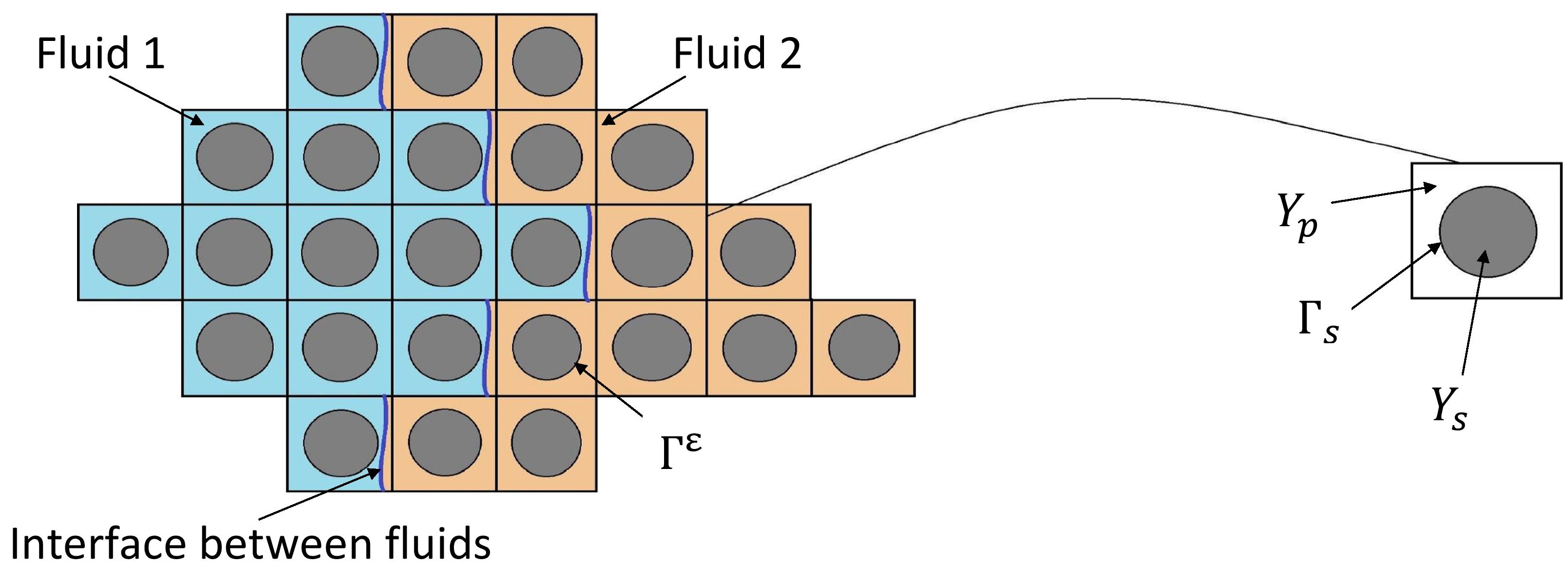
Figure 1: (left) Porous medium $\Omega=\Omega_{p}^{\varepsilon}\cup{\Omega}_{s}^{\varepsilon}$ as a periodic covering of the reference cell $Y=Y_{p}\cup Y_{s}$ (right). The blue interface is the microscopic boundary between two fluid phases occupying the pore space $\Omega_{p}^{\varepsilon}$.

We define the pore part as $\Omega_{p}^{\varepsilon}\coloneqq\bigcup_{\mathbf{k}\in{\mathbb{Z}}^{n}}Y_{p_{k}}\cap\Omega$, the solid part as $\Omega^{\varepsilon}_{s}\coloneqq\bigcup_{\mathbf{k}\in{\mathbb{Z}}^{n}}Y_{s_{k}}\cap\Omega=\Omega\backslash\Omega_{p}^{\varepsilon}$ and $\Gamma^{\varepsilon}\coloneqq\bigcup_{\mathbf{k}\in{\mathbb{Z}}^{n}}\Gamma_{s_{k}}$, where $Y_{p_{k}}\coloneqq\varepsilon{Y_{p}+k}$, $Y_{s_{k}}\coloneqq\varepsilon{Y_{s}+k}$ and $\Gamma_{s_{k}}=\bar{Y}_{p_{k}}\cap\bar{Y}_{s_{k}}$, cf. [8, 9]. Due to $Y$-periodicity, the characteristic function of the domain $\Omega_{p}^{\varepsilon}$ is given by $\chi_{\varepsilon}(x)=\chi\left(\frac{x}{\varepsilon}\right)$ and defined by $\chi_{\varepsilon}(x)\coloneqq 1$ for $y\in\Omega_{p}^{\varepsilon}$; 0 for $y\in\Omega-\Omega_{p}^{\varepsilon}$. We assume that $\Omega_{p}^{\varepsilon}$ is connected and has a sufficiently smooth boundary. We consider the situation where the pore part $\Omega_{p}^{\varepsilon}$ is occupied by the immiscible binary fluids separated by a microscopic interface of thickness $\varepsilon\lambda$ where $\lambda>0$ represented by the blue part in figure 1 and includes the surface tension effects on the motion of the interface. We model the flow of the fluid mixture at the pore-scale using a phase-field approach motivated by the system (1.2), cf. [8, 9]. If there is no confusion, we use the below-shortened notations in the subsequent sections: $\Omega_{S}\coloneqq S\times\Omega$, $\partial\Omega_{S}\coloneqq S\times\partial\Omega$, $\Omega^{\varepsilon}_{S}\coloneqq S\times\Omega^{\varepsilon}$, $\Omega^{\varepsilon}_{p,S}\coloneqq S\times\Omega^{\varepsilon}_{p}$ and $\partial\Omega^{\varepsilon}_{p,S}\coloneqq S\times\partial\Omega^{\varepsilon}_{p}$. The velocity of the fluid mixture is assumed to be $\mathbf{u}^{\varepsilon}=\mathbf{u}^{\varepsilon}(t,x)$, $(t,x)\in S\times\Omega_{p}^{\varepsilon}$ satisfying the evolutionary Stokes equation.

$$\partial_{t}c^{\varepsilon}+\varepsilon\mathbf{u}^{\varepsilon}.\nabla c^{\varepsilon} =\varepsilon^{2}\Delta w^{\varepsilon}, \Omega_{p,S}^{\varepsilon},$$ (1.5a)

$$w^{\varepsilon} =-\Delta c^{\varepsilon}+f(c^{\varepsilon}), \Omega_{p,S}^{\varepsilon},$$ (1.5b)

$$\partial_{n}c^{\varepsilon}=0, \quad\partial_{n}w^{\varepsilon}=0 \partial\Omega^{\varepsilon}_{p,S},$$ (1.5c)

$$\partial_{t}\mathbf{u}^{\varepsilon}-\mu\varepsilon^{2}\Delta\mathbf{u}^{\varepsilon}+\nabla p^{\varepsilon} =-\varepsilon\lambda c^{\varepsilon}\nabla w^{\varepsilon}, \Omega_{p,S}^{\varepsilon},$$ (1.5d)

$$\nabla.\mathbf{u}^{\varepsilon} =0, \Omega_{p,S}^{\varepsilon},$$ (1.5e)

$$\mathbf{u}^{\varepsilon} =0, \partial\Omega^{\varepsilon}_{p,S},$$ (1.5f)

$$c^{\varepsilon}(0,x)=c_{0}(x), \quad\mathbf{u}^{\varepsilon}(0,x)=\mathbf{u}_{0}(x), \Omega_{p}^{\varepsilon}.$$ (1.5g)

The chemical potential $w^{\varepsilon}$ and the order parameter $c^{\varepsilon}$, which plays the role of microscopic concentration, satisfy the Cahn-Hilliard equation. $p^{\varepsilon}$ is the fluid pressure. The term $\varepsilon\lambda c^{\varepsilon}\nabla w^{\varepsilon}$ models the surface tension forces which act on the microscopic interface between the fluids. Fluid density is taken to be $1$. Let the considered time interval be $S\coloneqq(0,T)$ with $0<T<+\infty$. The time variable is labelled with $t$ whereas $x$ and $y\coloneqq\frac{x}{\varepsilon}$ denote the slow (macroscopic) and rapid (microscopic) variables, respectively. The model under consideration leads to the system (1.5) of partial differential equations, where $\frac{\partial c^{\varepsilon}}{\partial\mathbf{n}}\eqqcolon\partial_{n}c^{\varepsilon}$, $\frac{\partial w^{\varepsilon}}{\partial\mathbf{n}}\eqqcolon\partial_{n}w^{\varepsilon}$. The scaling for the viscosity is such that the velocity $\mathbf{u}^{\varepsilon}$ has a nontrivial limit as $\varepsilon$ goes to zero. In (1.5b), $f(s)=-\theta_{0}s+\frac{\theta}{2}\ln\frac{1+s}{1-s}\eqqcolon F^{\prime}(s)$, where $F$ is as defined in (1.3). Here $\varepsilon^{2}$ is chosen to enter into the problem because we want to scale the velocity field $\mathbf{u}^{\varepsilon}$ so that it has a nontrivial limit as $\varepsilon$ goes to zero. We denote the problem (1.5a) - (1.5g) by $\mathcal{(P^{\varepsilon})}$.

2 Notations and function space setting

Let $\theta\in[0,1]$ and $1\leq r,s\leq\infty$ be such that $\frac{1}{r}+\frac{1}{s}=1$. Assume that $\Xi\in\{\Omega,\Omega_{p}^{\varepsilon},\Omega_{s}^{\varepsilon}\}$ and $l\in\mathbb{N}_{0}$, then as usual, $L^{r}(\Xi)$ and $H^{l,r}(\Xi)$ denote the Lebesgue and Sobolev spaces with their usual norms and are denoted by $||.||_{r}$ and $||.||_{l,r}$. Similarly, $C^{\theta}(\bar{\Xi})$, $(\cdot,\cdot)_{\theta,r}$ and $[\cdot,\cdot]_{\theta}$ are the Hölder, real- and complex-interpolation spaces respectively endowed with their standard norms, for definition one may refer to [19, 35]. $C^{\alpha}_{\#}(Y)$ denotes the set of all Y-periodic $\alpha$-times continuously differentiable functions in $y$ for $\alpha\in\mathbb{N}$. In particular, $C_{\#}(Y)$ is the space of all the Y-periodic continuous functions in $y$. The $C^{\infty}$-spaces are, as usual, equipped with their maximum norm, whereas the space of all continuous functions $C(\Xi)$ is furnished with supremum norm, cf. [19]. The extension and restriction operators are denoted by $E$ and $R$, respectively. The symbol $(.,.)_{H}$ represents the inner product on a Hilbert space H, and $||.||_{H}$ denotes the corresponding norm. For a Banach space $X$, $X^{*}$ denotes its dual and the duality pairing is denoted by $\langle.\;,\;.\rangle_{X^{*}\times X}$. For $p=2,\,H^{1,2}=H^{1}$ and $H^{1}_{0}(\Xi)^{*}=H^{-1}(\Xi)$, where subscript $0$ stands for zero trace. The symbols $\hookrightarrow$, $\hookrightarrow\hookrightarrow$, and $\underset{\hookrightarrow}{d}$ denote the continuous, compact and dense embeddings, respectively. We use the following notations for the function spaces:

$$\mathcal{U}=\{\mathbf{u}\in\mathcal{D}(\overline{\Omega})^{d}:\divergence\mathbf{u}=0,\mathbf{u}|_{\partial\Omega}=0\}, \mathcal{C}=\{c\in\mathcal{D}(\overline{\Omega}):\partial_{n}c=\partial_{n}\Delta c=0\text{ on }\partial\Omega\}.$$

We further define $L^{2}_{0}(\Omega^{\epsilon}_{p})=\{\zeta\in L^{2}(\Omega_{\epsilon}^{p}):\int_{\Omega_{\epsilon}^{p}}\zeta dx=0\}$, $\mathcal{U}_{r}(\Omega)\coloneqq\overline{\mathcal{U}}^{\mathbb{H}^{r}(\Omega)}$, $\mathcal{C}_{r}(\Omega)\coloneqq\overline{\mathcal{C}}^{H^{r}(\Omega)}$, $\mathcal{U}(\Omega)=\overline{\mathcal{U}}^{\mathbb{L}^{2}(\Omega)}$, $\mathcal{C}(\Omega)=\overline{\mathcal{C}}^{L^{2}(\Omega)}$, with $\mathbb{L}^{2}(\Omega)=L^{2}(\Omega)^{d}$ and $\mathbb{H}^{r}(\Omega)=H^{r}(\Omega)^{d}$. The spaces $\mathcal{C}_{r}^{\prime}(\Omega_{p}^{\varepsilon})$ and $\mathcal{U}_{r}^{\prime}(\Omega_{p}^{\varepsilon})$ represent the dual of $\mathcal{C}_{r}(\Omega_{p}^{\varepsilon})$ and $\mathcal{U}_{r}(\Omega_{p}^{\varepsilon})$ with respect to their standard norms. Also,

$$\mathfrak{C}^{\varepsilon}\coloneqq\left\{c^{\varepsilon}:c^{\varepsilon}\in L^{\infty}(S;\mathcal{C}_{1}(\Omega_{p}^{\varepsilon}))\cap L^{2}_{\text{loc}}(S;\mathcal{C}_{3}(\Omega_{p}^{\varepsilon}))\right\},\mathfrak{W}^{\varepsilon}\coloneqq\left\{w^{\varepsilon}:w^{\varepsilon}\in L^{2}_{\text{loc}}(S;\mathcal{C}_{1}(\Omega_{p}^{\varepsilon}))\right\},$$

$$\mathfrak{V}^{\varepsilon}\coloneqq\left\{\mathbf{u}^{\varepsilon}:\mathbf{u}^{\varepsilon}\in L^{\infty}(S;\mathcal{U}(\Omega_{p}^{\varepsilon}))\cap L^{2}_{\text{loc}}(S;\mathcal{U}_{1}(\Omega_{p}^{\varepsilon}))\right\},\mathfrak{P}^{\varepsilon}\coloneqq\left\{p^{\varepsilon}:p^{\varepsilon}\in W^{-1,\infty}(S;L_{0}^{2}(\Omega_{p}^{\varepsilon}))\right\},$$

and $\mathfrak{C}^{\varepsilon}_{\delta}\coloneqq\left\{c^{\varepsilon}:c^{\varepsilon}\in L^{\infty}(S;\mathcal{C}_{1}(\Omega_{p}^{\varepsilon}))\cap L^{2}_{\text{loc}}(S;\mathcal{C}_{2}(\Omega_{p}^{\varepsilon}))\right\}$ (to address in definition 3.2).

2.1 Main assumptions

The function $F$ is assumed to satisfy the below assumptions, cf.[11].

1. $F$ is of class $\mathbb{C}^{2}$, and $F\geq 0$ as physically-relevant functions $F$ are always bounded from below, and so the equations remain unchanged by adding a constant to $F$.

2. $\exists~{}\mathcal{K}_{1},\mathcal{K}_{2}>0$ such that $|f(x)|\leq\mathcal{K}_{1}|x|^{p}+\mathcal{K}_{2}$, $|f^{\prime}(x)|\leq\mathcal{K}_{1}|x|^{p-1}+\mathcal{K}_{2}$, $\forall x\in\mathbb{R}$, where $1\leq p<+\infty$ if $d=2$ and $1\leq p\leq 3$ if $d=3$.

3. $\forall\gamma\in\mathbb{R}$, $\exists~{}\mathcal{K}_{3}(\gamma)>0$, $\mathcal{K}_{4}(\gamma)\geq 0$ such that $(x-\gamma)f(x)\geq\mathcal{K}_{3}F(x)-\mathcal{K}_{4}(\gamma)$, $\forall x\in\mathbb{R}$.

4. $\exists~{}\mathcal{K}_{5}$ such that $f^{\prime}\geq-\mathcal{K}_{5}$, $\forall x\in\mathbb{R}$, where $0\leq\mathcal{K}_{5}<\frac{1}{4}$.

Also, we make the following assumptions to analyze $\mathcal{(P^{\varepsilon})}$.

1. for all $x\in\Omega$, $\mathbf{u_{0}}\geq 0$.

2. $\mathbf{u_{0}}\in L^{\infty}(\Omega)\cap H^{1}(\Omega)$, $c_{0}\in L^{\infty}(\Omega)\cap H^{1}(\Omega)$ such that
   $\sup_{\varepsilon>0}||\mathbf{u_{0}}||_{L^{\infty}(\Omega)\cap H^{1}(\Omega)}<\infty,$ $\sup_{\varepsilon>0}||c_{0}||_{L^{\infty}(\Omega)\cap H^{1}(\Omega)}<\infty$.

Remark 2.1.

The positive constant $C$ is estimated in terms of $\Omega$ and the parameters $\mathcal{K}_{1},\mathcal{K}_{2},\ldots,\mathcal{K}_{6}$ of the system throughout the paper (see section 2.1). Any further dependence will be explicitly pointed out when necessary. Notably, the constant $C$ is independent of the scale parameter $\varepsilon$.

3 Existence of the model $\mathcal{(P^{\varepsilon})}$

In this section, the weak formulation of the problem $\mathcal{(P^{\varepsilon})}$ is defined in section 3.1 at first. Next, we rigorously prove the existence of the model equations (1.5) in section 3.2.

3.1 Weak formulation of $\mathcal{(P^{\varepsilon})}$

Definition 3.1 (Weak solution of $\mathcal{(P^{\varepsilon})}$).

Let assumptions A1-A6 be satisfied. A quadruple $(c^{\varepsilon},w^{\varepsilon},\mathbf{u}^{\varepsilon},p^{\varepsilon})\in\mathfrak{C}^{\varepsilon}\times\mathfrak{W}^{\varepsilon}\times\mathfrak{V}^{\varepsilon}\times\mathfrak{P}^{\varepsilon}$ is a weak solution of $\mathcal{(P^{\varepsilon})}$ if:

1. $c^{\varepsilon},\mathbf{u}^{\varepsilon}$ satisfy $c^{\varepsilon}\in\mathfrak{C}^{\varepsilon}\cap C^{0}\left([0,T);\mathcal{C}_{1}(\Omega_{p}^{\varepsilon})\right)$, $\mathbf{u}^{\varepsilon}\in\mathfrak{V}^{\varepsilon}\cap C^{0}\left([0,T);\mathcal{U}^{\prime}_{\frac{d-2}{4}}(\Omega_{p}^{\varepsilon})\right),$

2. $(c^{\varepsilon},\mathbf{u}^{\varepsilon})(0,x)=(c_{0},\mathbf{u}_{0})(x)$ for all $x\in\Omega_{p}^{\varepsilon}$,

3. for any $\phi$ in $\mathcal{C}_{1}(\Omega_{p}^{\varepsilon})$

   $$\left\langle\frac{\mathop{}\!\mathrm{d}c^{\varepsilon}}{\mathop{}\!\mathrm{d}t},\phi\right\rangle+\varepsilon^{2}\int_{\Omega_{p}^{\varepsilon}}\nabla w^{\varepsilon}\cdot\nabla\phi\,dx-\varepsilon\int_{\Omega_{p}^{\varepsilon}}c^{\varepsilon}(\mathbf{u}^{\varepsilon}\cdot\nabla\phi)\,dx=0\quad in\;\mathcal{D}([0,T)),$$ (3.1)

4. for any $\psi$ in $\mathcal{C}_{1}(\Omega_{p}^{\varepsilon})$

   $$\int_{\Omega_{p}^{\varepsilon}}w^{\varepsilon}\psi\,dx=\int_{\Omega_{p}^{\varepsilon}}\nabla c^{\varepsilon}\cdot\nabla\psi\,dx+\int_{\Omega_{p}^{\varepsilon}}f(c^{\varepsilon})\psi\,dx\qquad in\;\mathcal{D}([0,T)).$$ (3.2)

5. for any $\eta$ in $\mathcal{U}_{1}(\Omega_{p}^{\varepsilon})$

   $$\left\langle\frac{\mathop{}\!\mathrm{d}\mathbf{u}^{\varepsilon}}{\mathop{}\!\mathrm{d}t},\eta\right\rangle+\mu\varepsilon^{2}\int_{\Omega_{p}^{\varepsilon}}\nabla\mathbf{u}^{\varepsilon}\colon\nabla\eta\,dx=-\varepsilon\lambda\int_{\Omega_{p}^{\varepsilon}}c^{\varepsilon}(\eta\cdot\nabla w^{\varepsilon})\,dx\quad in\;\mathcal{D}([0,T)),$$ (3.3)

where $\mathcal{U}_{1}(\Omega_{p}^{\varepsilon}),\mathcal{C}_{1}(\Omega_{p}^{\varepsilon})$ are as introduced in the section 2. We associate a pressure $p^{\varepsilon}\coloneqq\partial_{t}P^{\varepsilon}$ with each weak solution $(c^{\varepsilon},w^{\varepsilon},\mathbf{u}^{\varepsilon})$, which satisfies (1.5d) in the distributional sense (3.2) cf. [8].

Definition 3.2 (Weak solution of $\mathcal{(P^{\varepsilon}_{\delta})}$).

Let $d=2$ and the assumptions A1-A6 be satisfied. A triple $(c_{\delta}^{\varepsilon},\mathbf{u}_{\delta}^{\varepsilon},p_{\delta}^{\varepsilon})\in\mathfrak{C}^{\varepsilon}_{\delta}\times\mathfrak{V}^{\varepsilon}\times\mathfrak{P}^{\varepsilon}$ is a weak solution of $\mathcal{(P^{\varepsilon}_{\delta})}$ stated in (3.31)-(3.33) if:

1. $\mathbf{u}_{\delta}^{\varepsilon},c_{\delta}^{\varepsilon}$ satisfy $c_{\delta}^{\varepsilon}\in\mathfrak{C}^{\varepsilon}_{\delta}\cap C^{0}\left([0,T);\mathcal{C}_{\frac{1}{2}}(\Omega_{p}^{\varepsilon}\right)$, $\mathbf{u}_{\delta}^{\varepsilon}\in\mathfrak{V}^{\varepsilon}\cap C^{0}\left([0,T);\mathcal{U}^{\prime}_{\frac{d-2}{4}}(\Omega_{p}^{\varepsilon})\right),$

2. $(\mathbf{u}_{\delta}^{\varepsilon},c_{\delta}^{\varepsilon})(0,x)=(\mathbf{u}_{0},c_{0})(x)$ for all $x\in\Omega_{p}^{\varepsilon}$,

3. for any $\phi$ in $\mathcal{C}_{3}(\Omega_{p}^{\varepsilon})$

   $$\left\langle\frac{\mathop{}\!\mathrm{d}c_{\delta}^{\varepsilon}}{\mathop{}\!\mathrm{d}t},\phi\right\rangle+\varepsilon^{2}\int_{\Omega_{p}^{\varepsilon}}\Delta c_{\delta}^{\varepsilon}\cdot\Delta\phi\,dx+\varepsilon^{2}\int_{\Omega_{p}^{\varepsilon}}f_{\delta}^{\prime}(c_{\delta}^{\varepsilon})\nabla c_{\delta}^{\varepsilon}\cdot\nabla\phi\,dx-\varepsilon\int_{\Omega_{p}^{\varepsilon}}c_{\delta}^{\varepsilon}(\mathbf{u}_{\delta}^{\varepsilon}\cdot\nabla\phi)\,dx=0\quad in\,\mathcal{D}([0,T)),$$ (3.4)

4. for any $\eta$ in $\mathcal{U}_{1}(\Omega_{p}^{\varepsilon})$

   $$\left\langle\frac{\mathop{}\!\mathrm{d}\mathbf{u}_{\delta}^{\varepsilon}}{\mathop{}\!\mathrm{d}t},\eta\right\rangle+\mu\varepsilon^{2}\int_{\Omega_{p}^{\varepsilon}}\nabla\mathbf{u}_{\delta}^{\varepsilon}\colon\nabla\eta\,dx=-\varepsilon\lambda\int_{\Omega_{p}^{\varepsilon}}\Delta c_{\delta}^{\varepsilon}(\eta\cdot\nabla c_{\delta}^{\varepsilon})\,dx\quad in\;\mathcal{D}([0,T)).$$ (3.5)

Remark 3.1.

The weak formulation for $w^{\varepsilon}$ does not appear in the second case, as we replaced $w_{\delta}^{\varepsilon}~{}\nabla c_{\delta}^{\varepsilon}$ by $-\Delta c_{\delta}^{\varepsilon}\nabla c_{\delta}^{\varepsilon}$ in the last term of 3.5 as the term $f_{\delta}(c_{\delta}^{\varepsilon})\nabla c_{\delta}^{\varepsilon}$ is the gradient of $F_{\delta}(c_{\delta}^{\varepsilon})$ which can be considered as a part of the pressure gradient.

3.2 Existence of weak solutions

Theorem 3.1.

Let $d=2,3$. Assume that $c_{0}\in\mathcal{C}_{1}(\Omega_{p}^{\varepsilon})$, $\mathbf{u}_{0}\in\mathcal{U}(\Omega_{p}^{\varepsilon})$ with $\norm{c_{0}}_{L^{\infty}(\Omega)}\leq 1$ and $\absolutevalue{m(c_{0})}<1$. Also, $F$ satisfies the assumptions A1-A4 stated in section 2.1, then for any $T>0$, there exists a global weak solution $(\mathbf{u}^{\varepsilon},c^{\varepsilon},w^{\varepsilon},p^{\varepsilon})$ to the problem $\mathcal{(P^{\varepsilon})}$ in the sense of definition 3.1 which satisfies

$$\norm{c^{\varepsilon}-\overline{c^{\varepsilon}}}_{L^{\infty}(S;\mathcal{C}_{1}(\Omega_{p}^{\varepsilon})}+\norm{\mathbf{u}^{\varepsilon}}_{L^{\infty}(S;\mathcal{U}(\Omega_{p}^{\varepsilon}))}+\norm{w^{\varepsilon}}_{L^{2}(S;\mathcal{C}(\Omega_{p}^{\varepsilon}))}+\norm{\partial_{t}c^{\varepsilon}}_{L^{2}(S;\mathcal{C}_{1}^{\prime}(\Omega_{p}^{\varepsilon}))}+\norm{\partial_{t}\mathbf{u}^{\varepsilon}}_{L^{2}(S;\mathcal{U}_{1}^{\prime}(\Omega_{p}^{\varepsilon}))}$$

$$+\frac{\varepsilon}{2}\norm{\nabla w^{\varepsilon}}_{L^{2}(S\times\Omega_{p}^{\varepsilon})^{d}}+\norm{c^{\varepsilon}-m(c^{\varepsilon})}_{L^{2}(S;\mathcal{C}(\Omega_{p}^{\varepsilon}))}+\sqrt{\mu}\varepsilon\norm{\nabla\mathbf{u}^{\varepsilon}}_{L^{2}(S;\mathcal{U}(\Omega_{p}^{\varepsilon})))}+\norm{c^{\varepsilon}-m(c^{\varepsilon})}_{L^{2}(S;\mathcal{C}_{2}(\Omega_{p}^{\varepsilon}))}$$

$$\leq C\left(c_{0},\mathbf{u}_{0},T\right),$$ (3.6)

where the constant $C$ is independent of $\varepsilon$.

Furthermore, to prove a result concerning strong solutions to $\mathcal{(P^{\varepsilon})}$, we assume that $F$ is of $C^{3}$-class, and there exists a non-negative $\mathcal{K}_{6}$ such that

$$\absolutevalue{f^{\prime\prime}(x)}\leq\mathcal{K}_{6}\left(1+\absolutevalue{x}^{r}\right),~{}~{}\forall x\in\mathbb{R},$$ (3.7)

where $r<3$ if $d=3$ and $r<+\infty$ if $d=2$.

Proof.

To prove theorem 3.1, we only need to show that there exists a triple $(c^{\varepsilon},w^{\varepsilon},\mathbf{u}^{\varepsilon})\in\left(\mathfrak{C}^{\varepsilon},\mathfrak{W}^{\varepsilon},\mathfrak{V}^{\varepsilon}\right)$ satisfying the initial conditions $c^{\varepsilon}(0,x)=c_{0}(x)$, $\mathbf{u}^{\varepsilon}(0,x)=\mathbf{u}_{0}(x)$ and the weak formuation (3.1)-(3.3). To show this, we employ the Galerkin approximation. We use $(\xi_{i})_{i\geq 1}$, the family of the eigenfunctions of the operator $-\Delta$ with the boundary conditions (1.5c) as a Galerkin base in $\mathcal{C}_{1}(\Omega_{p}^{\varepsilon})$, and $(\zeta_{i})_{i\geq 1}$, the family of eigenfunctions of the Stokes operator $A$ (see definition A.1) as a Galerkin base in $\mathcal{U}_{1}(\Omega_{p}^{\varepsilon})$. We fix $\xi_{1}$ to be 1. Also, we remark that $(\xi_{i})_{i\geq 1}$ are orthogonal both in $\mathcal{C}(\Omega_{p}^{\varepsilon})$ and $\mathcal{C}_{1}(\Omega_{p}^{\varepsilon})$. We define the $n$-dimensional spaces $\Xi_{n}=\{\xi_{1},\xi_{2},\ldots,\xi_{n}\},Z_{n}=\{\zeta_{1},\zeta_{2},\ldots,\zeta_{n}\}$ and $P_{\Xi_{n}}$, $P_{Z_{n}}$ the orthogonal projectors on these spaces in $\mathcal{C}_{1}(\Omega_{p}^{\varepsilon})$, $\mathcal{U}_{1}(\Omega_{p}^{\varepsilon})$, respectively. Now we seek three functions of the form:

$$c_{n}^{\varepsilon}=\sum_{i=1}^{n}\alpha_{i}(t)\xi_{i}\in\Xi_{n}, w_{n}^{\varepsilon}=\sum_{i=1}^{n}\beta_{i}(t)\xi_{i}\in\Xi_{n}, \mathbf{u}_{n}^{\varepsilon}=\sum_{i=1}^{n}\gamma_{i}(t)\zeta_{i}\in Z_{n}$$

where $\alpha_{i},\beta_{i},\gamma_{i}$ are real-valued $C^{1}$ functions such that $c_{n}^{\varepsilon}(0)=P_{\Xi_{n}}(0)$, $\mathbf{u}_{n}^{\varepsilon}(0)=P_{Z_{n}}(0)$ and

$$\left\langle\frac{\mathop{}\!\mathrm{d}c^{\varepsilon}}{\mathop{}\!\mathrm{d}t},\phi\right\rangle+\varepsilon^{2}\int_{\Omega_{p}^{\varepsilon}}\nabla w_{n}^{\varepsilon}\cdot\nabla\phi\,dx-\varepsilon\int_{\Omega_{p}^{\varepsilon}}c_{n}^{\varepsilon}(\mathbf{u}_{n}^{\varepsilon}\cdot\nabla\phi)\,dx=0$$ (3.8)

$$\int_{\Omega_{p}^{\varepsilon}}w_{n}^{\varepsilon}\psi\,dx=\int_{\Omega_{p}^{\varepsilon}}\nabla c_{n}^{\varepsilon}\cdot\nabla\psi\,dx+\int_{\Omega_{p}^{\varepsilon}}f(c_{n}^{\varepsilon})\psi\,dx$$ (3.9)

$$\left\langle\frac{\mathop{}\!\mathrm{d}\mathbf{u}^{\varepsilon}}{\mathop{}\!\mathrm{d}t},\eta\right\rangle+\mu\varepsilon^{2}\int_{\Omega_{p}^{\varepsilon}}\nabla\mathbf{u}_{n}^{\varepsilon}\colon\nabla\eta\,dx=-\varepsilon\lambda\int_{\Omega_{p}^{\varepsilon}}c_{n}^{\varepsilon}(\eta\cdot\nabla w_{n}^{\varepsilon})\,dx$$ (3.10)

in $\mathcal{D}([0,T))$ for all $\phi,\psi\in\mathcal{C}_{1}(\Omega_{p}^{\varepsilon})$ and $\eta\in\mathcal{U}_{1}(\Omega_{p}^{\varepsilon})$. The function $f$ in (3.9) is locally Lipschitz, which leads to the equivalency of the system of model equations to a Cauchy problem for a system of ordinary differential equations in the unknowns $\alpha_{i}$, $\beta_{i}$, $\gamma_{i}$. The Cauchy-Lipschitz theorem ensures this system has a unique solution into an interval $[0,t_{n})$, $t_{n}>0$.
Next, we replace $\phi$ by $\xi_{1}$ in (3.8) as a test function. We find that for all $n\geq 1$ and $t_{n}\in[0,t_{n})$, we have

$$\frac{\mathop{}\!\mathrm{d}}{\mathop{}\!\mathrm{d}t}m(c_{n}^{\varepsilon})=\frac{1}{\absolutevalue{\Omega_{p}^{\varepsilon}}}\int_{\Omega_{p}^{\varepsilon}}\frac{\partial c_{n}^{\varepsilon}}{\partial t}\xi_{1}\,dx=0\quad\implies m(c_{n}^{\varepsilon})(t)=m(c_{n}^{\varepsilon})(0)=m(P_{\Xi_{n}}(c_{0}))=m(c_{0}),$$

where $m(c_{n}^{\varepsilon})\coloneqq\frac{1}{\absolutevalue{\Omega}}\int_{\Omega}c_{n}^{\varepsilon}(x)\,dx$, i.e., the average $m(c_{n}^{\varepsilon})$ depends only on the initial data $c_{0}$ and is independent of $t$ and $n$. We derive some a-priori estimates to show that $t_{n}\rightarrow T$ for every $n\geq 1$. The estimates will ultimately lead to showing that the sequences $(c_{n}^{\varepsilon})$, $(w_{n}^{\varepsilon})$ and $(\mathbf{u}_{n}^{\varepsilon})$ are bounded in the appropriate function spaces. We use $w_{n}^{\varepsilon}\in\Xi_{n}$ as a test function in (3.8) to get

$$\left\langle\frac{\mathop{}\!\mathrm{d}c^{\varepsilon}}{\mathop{}\!\mathrm{d}t},w_{n}^{\varepsilon}\right\rangle+\varepsilon^{2}\int_{\Omega_{p}^{\varepsilon}}\absolutevalue{\nabla w_{n}^{\varepsilon}}^{2}\,dx-\varepsilon\int_{\Omega_{p}^{\varepsilon}}c_{n}^{\varepsilon}(\mathbf{u}_{n}^{\varepsilon}\cdot\nabla w_{n}^{\varepsilon})\,dx=0.$$ (3.11)

We substitute the expression of $w_{n}^{\varepsilon}$ using (1.5b) in the first term of (3.11), and get

$$\left\langle\frac{\mathop{}\!\mathrm{d}c^{\varepsilon}}{\mathop{}\!\mathrm{d}t},\left\{-\Delta c_{n}^{\varepsilon}+P_{\Xi_{n}}\left(f(c_{n}^{\varepsilon})\right)\right\}\right\rangle+\varepsilon^{2}\int_{\Omega_{p}^{\varepsilon}}\absolutevalue{\nabla w_{n}^{\varepsilon}}^{2}\,dx-\varepsilon\int_{\Omega_{p}^{\varepsilon}}c_{n}^{\varepsilon}(\mathbf{u}_{n}^{\varepsilon}\cdot\nabla w_{n}^{\varepsilon})\,dx=0,$$

i.e., $$\frac{\mathop{}\!\mathrm{d}}{\mathop{}\!\mathrm{d}t}\left\{\frac{1}{2}\norm{\nabla c_{n}^{\varepsilon}}_{L^{2}(\Omega_{p}^{\varepsilon})}^{2}+\int_{\Omega_{p}^{\varepsilon}}F(c_{n}^{\varepsilon})\,dx\right\}+\varepsilon^{2}\int_{\Omega_{p}^{\varepsilon}}\absolutevalue{\nabla w_{n}^{\varepsilon}}^{2}\,dx-\varepsilon\int_{\Omega_{p}^{\varepsilon}}c_{n}^{\varepsilon}(\mathbf{u}_{n}^{\varepsilon}\cdot\nabla w_{n}^{\varepsilon})\,dx=0.$$ (3.12)

Next, we consider $\mathbf{u}_{n}^{\varepsilon}$ as a test function in (3.10).

$$\frac{\mathop{}\!\mathrm{d}}{\mathop{}\!\mathrm{d}t}\left\{\frac{1}{2}\norm{\mathbf{u}_{n}^{\varepsilon}}_{L^{2}(\Omega_{p}^{\varepsilon})}^{2}\right\}+\mu\varepsilon^{2}\int_{\Omega_{p}^{\varepsilon}}\absolutevalue{\nabla\mathbf{u}_{n}^{\varepsilon}}^{2}\,dx=-\varepsilon\lambda\int_{\Omega_{p}^{\varepsilon}}(c_{n}^{\varepsilon}-m(c_{n}^{\varepsilon}))(\mathbf{u}_{n}^{\varepsilon}\cdot\nabla w_{n}^{\varepsilon})\,dx.$$ (3.13)

Since $\mathbf{u}_{n}^{\varepsilon}$ is divergence-free, additionally using (1.5c), we find that

$$\varepsilon\lambda\int_{\Omega_{p}^{\varepsilon}}\mathbf{u}_{n}^{\varepsilon}\cdot\nabla w_{n}^{\varepsilon}\,dx\implies\varepsilon\lambda\int_{\Omega_{p}^{\varepsilon}}\divergence{w_{n}^{\varepsilon}\mathbf{u}_{n}^{\varepsilon}}\,dx\implies\varepsilon\lambda\int_{\partial\Omega_{p}^{\varepsilon}}w_{n}^{\varepsilon}\mathbf{u}_{n}^{\varepsilon}\cdot\mathbf{n}\,dx\implies 0.$$ (3.14)

We use (3.14) while adding (3.2), (3.13) and get

$$\frac{\mathop{}\!\mathrm{d}}{\mathop{}\!\mathrm{d}t}\left\{\frac{1}{2}\norm{\nabla c_{n}^{\varepsilon}}_{L^{2}(\Omega_{p}^{\varepsilon})}^{2}+\frac{1}{2}\norm{\mathbf{u}_{n}^{\varepsilon}}_{L^{2}(\Omega_{p}^{\varepsilon})}^{2}+\int_{\Omega_{p}^{\varepsilon}}F(c_{n}^{\varepsilon})\,dx\right\}+\varepsilon^{2}\norm{\nabla w_{n}^{\varepsilon}}_{L^{2}(\Omega_{p}^{\varepsilon})}^{2}+\mu\varepsilon^{2}\norm{\nabla\mathbf{u}_{n}^{\varepsilon}}_{L^{2}(\Omega_{p}^{\varepsilon})}^{2}=0.$$ (3.15)

Next, we use $c_{n}^{\varepsilon}-m(c_{n}^{\varepsilon})\xi_{1}$ as a test function in (3.9).

$$\left\langle w_{n}^{\varepsilon},c_{n}^{\varepsilon}-m(c_{n}^{\varepsilon})\right\rangle=\int_{\Omega_{p}^{\varepsilon}}\nabla c_{n}^{\varepsilon}\cdot\nabla(c_{n}^{\varepsilon}-m(c_{0}))\,dx+\left\langle f(c_{n}^{\varepsilon}),c_{n}^{\varepsilon}-m(c_{0})\right\rangle,$$

i.e., $$\left\langle w_{n}^{\varepsilon}-m(w_{n}^{\varepsilon}),c_{n}^{\varepsilon}-m(c_{n}^{\varepsilon})\right\rangle=\norm{\nabla c_{n}^{\varepsilon}}_{L^{2}(\Omega_{p}^{\varepsilon})}^{2}+\left\langle f(c_{n}^{\varepsilon}),c_{n}^{\varepsilon}-m(c_{0})\right\rangle.$$ (3.16)

Note that $\xi_{1}$ is taken to be 1 when required in the calculation. We use Young’s inequality and Lemma A.3 for the domain $\Omega_{p}^{\varepsilon}$ along with the assumption A3 to find

$$\frac{\varepsilon^{2}}{4}\norm{\nabla w_{n}^{\varepsilon}}_{L^{2}(\Omega_{p}^{\varepsilon})}^{2}\geq\frac{3}{4}\norm{\nabla c_{n}^{\varepsilon}}_{L^{2}(\Omega_{p}^{\varepsilon})}^{2}+\mathcal{K}_{3}\left(m(c_{0})\right)\int_{\Omega_{p}^{\varepsilon}}F(c_{n}^{\varepsilon})\,dx-\absolutevalue{\Omega_{p}^{\varepsilon}}\mathcal{K}_{4}\left(m(c_{0})\right),$$ (3.17)

where $\mathcal{K}_{3}$ and $\mathcal{K}_{4}$ are positive real-valued functions introduced in section 2.1. We multiply (1.5b) by $-\Delta c_{n}^{\varepsilon}$, which, after using integration by parts, leads to

$$\left\langle\nabla w_{n}^{\varepsilon},\nabla c_{n}^{\varepsilon}\right\rangle=\norm{\Delta c_{n}^{\varepsilon}}_{L^{2}(\Omega_{p}^{\varepsilon})}^{2}+\int_{\Omega_{p}^{\varepsilon}}f^{\prime}(c_{n}^{\varepsilon})\absolutevalue{\nabla c_{n}^{\varepsilon}}^{2}\,dx.$$

Again, Young’s inequality and the assumption A4 lead to

$$\frac{\varepsilon^{2}}{2}\norm{\nabla w_{n}^{\varepsilon}}_{L^{2}(\Omega_{p}^{\varepsilon})}^{2}\geq\norm{\Delta c_{n}^{\varepsilon}}_{L^{2}(\Omega_{p}^{\varepsilon})}^{2}-\left\{\frac{1}{2}+\mathcal{K}_{5}\right\}\norm{\nabla c_{n}^{\varepsilon}}_{L^{2}(\Omega_{p}^{\varepsilon})}^{2},$$ (3.18)

for some non-negative real numbers $\mathcal{K}_{5}$. We add the estimates (3.17) and (3.18) to get

$$\frac{3}{4}\varepsilon^{2}\norm{\nabla w_{n}^{\varepsilon}}_{L^{2}(\Omega_{p}^{\varepsilon})}^{2}\geq\frac{3}{4}\norm{\nabla c_{n}^{\varepsilon}}_{L^{2}(\Omega_{p}^{\varepsilon})}^{2} +\norm{\Delta c_{n}^{\varepsilon}}_{L^{2}(\Omega_{p}^{\varepsilon})}^{2}-\left\{\frac{1}{2}+\mathcal{K}_{5}\right\}\norm{\nabla c_{n}^{\varepsilon}}_{L^{2}(\Omega_{p}^{\varepsilon})}^{2}$$

$$+\mathcal{K}_{3}\left(m(c_{0})\right)\int_{\Omega_{p}^{\varepsilon}}F(c_{n}^{\varepsilon})\,dx-\absolutevalue{\Omega_{p}^{\varepsilon}}\mathcal{K}_{4}\left(m(c_{0})\right).$$

Now we can say that there exist $C_{1}$, $C_{2}>0$ depending on $\mathcal{K}_{5}$ such that

$$\varepsilon^{2}\norm{\nabla w_{n}^{\varepsilon}}_{L^{2}(\Omega_{p}^{\varepsilon})}^{2} \geq\frac{1}{4}\varepsilon^{2}\norm{\nabla w_{n}^{\varepsilon}}_{L^{2}(\Omega_{p}^{\varepsilon})}^{2}+C_{1}\norm{\nabla c_{n}^{\varepsilon}}_{L^{2}(\Omega_{p}^{\varepsilon})}^{2}+\norm{\Delta c_{n}^{\varepsilon}}_{L^{2}(\Omega_{p}^{\varepsilon})}^{2}$$

$$+\mathcal{K}_{3}\left(m(c_{0})\right)\int_{\Omega_{p}^{\varepsilon}}F(c_{n}^{\varepsilon})\,dx-C_{2}\mathcal{K}_{4}\left(m(c_{0})\right).$$ (3.19)

From (3.2) and (3.2), we obtain

$$\frac{\mathop{}\!\mathrm{d}}{\mathop{}\!\mathrm{d}t}\left\{\frac{1}{2}\norm{\nabla c_{n}^{\varepsilon}}_{L^{2}(\Omega_{p}^{\varepsilon})}^{2}+\frac{1}{2}\norm{\mathbf{u}_{n}^{\varepsilon}}_{L^{2}(\Omega_{p}^{\varepsilon})}^{2}+\int_{\Omega_{p}^{\varepsilon}}F(c_{n}^{\varepsilon})\,dx\right\}+C_{1}\norm{\nabla c_{n}^{\varepsilon}}_{L^{2}(\Omega_{p}^{\varepsilon})}^{2}+\norm{\Delta c_{n}^{\varepsilon}}_{L^{2}(\Omega_{p}^{\varepsilon})}^{2}$$

$$+\frac{1}{4}\varepsilon^{2}\norm{\nabla w_{n}^{\varepsilon}}_{L^{2}(\Omega_{p}^{\varepsilon})}^{2}+\mathcal{K}_{3}\left(m(c_{0})\right)\int_{\Omega_{p}^{\varepsilon}}F(c_{n}^{\varepsilon})\,dx+\mu\varepsilon^{2}\norm{\nabla\mathbf{u}_{n}^{\varepsilon}}_{L^{2}(\Omega_{p}^{\varepsilon})}^{2}\leq C_{2}\mathcal{K}_{4}\left(m(c_{0})\right).$$ (3.20)

We define $y_{n}(t)$ as follows: $y_{n}(t)=\frac{1}{2}\norm{\nabla c_{n}^{\varepsilon}}_{L^{2}(\Omega_{p}^{\varepsilon})}^{2}+\frac{1}{2}\norm{\mathbf{u}_{n}^{\varepsilon}}_{L^{2}(\Omega_{p}^{\varepsilon})}^{2}+\int_{\Omega_{p}^{\varepsilon}}F(c_{n}^{\varepsilon})\,dx.$ For small non-negative $\kappa$, we obtain

$$y_{n}^{\prime}(t)+\kappa y_{n}(t)\leq C\mathcal{K}_{4}(m(c_{0})).$$

Following the positivity of $F$ from assumption A1, Gronwall–Bellman inequality argument shows that $t_{n}\rightarrow+\infty$ for every $n\geq 1$. Additionally, we find

$$y_{n}(t)\leq y_{n}(0)+\kappa^{-1}\left\{C\mathcal{K}_{4}\left(m(c_{0})\right)\right\},~{}~{}\forall t\geq 0.$$ (3.21)

According to the definition, $P_{\Xi_{n}}$ and $P_{Z_{n}}$ are orthogonal projectors in the spaces $L^{2}$ and $\mathbb{H}^{1}$. This fact along with the assumptions 2.1, (3.7) and the embedding $\mathbb{H}^{1}\subset\mathbb{L}^{p}$ where $p$ is chosen as in A2, yield

$$y_{n}(0) =\frac{1}{2}\norm{\nabla P_{\Xi_{n}}(c_{0})}_{L^{2}(\Omega_{p}^{\varepsilon})}^{2}+\frac{1}{2}\norm{P_{Z_{n}}(\mathbf{u}_{0})}_{L^{2}(\Omega_{p}^{\varepsilon})}^{2}+\int_{\Omega_{p}^{\varepsilon}}F\left(P_{\Xi_{n}}(c_{0})\right)\,dx$$

$$\leq\frac{1}{2}\norm{\nabla c_{0}}_{L^{2}(\Omega_{p}^{\varepsilon})}^{2}+\frac{1}{2}\norm{\mathbf{u}_{0}}_{L^{2}(\Omega_{p}^{\varepsilon})}^{2}+{\mathcal{K}_{3}\left(m(c_{0})\right)}^{-1}\left\{\absolutevalue{\Omega_{p}^{\varepsilon}}\mathcal{K}_{4}\left(m(c_{0})\right)+\int_{\Omega_{p}^{\varepsilon}}\absolutevalue{P_{\Xi_{n}}(c_{0})-m(c_{0})}\absolutevalue{f(P_{\Xi_{n}}(c_{0}))}\right\}$$

$$\leq\frac{1}{2}\norm{\nabla c_{0}}_{L^{2}(\Omega_{p}^{\varepsilon})}^{2}+\frac{1}{2}\norm{\mathbf{u}_{0}}_{L^{2}(\Omega_{p}^{\varepsilon})}^{2}$$

$$+{\mathcal{K}_{3}\left(m(c_{0})\right)}^{-1}\left\{\absolutevalue{\Omega_{p}^{\varepsilon}}\mathcal{K}_{4}\left(m(c_{0})\right)+\norm{P_{\Xi_{n}}\left(c_{0}-m(c_{0})\right)}_{L^{2}(\Omega_{p}^{\varepsilon})}\norm{\mathcal{K}_{1}+\mathcal{K}_{2}\absolutevalue{P_{\Xi_{n}}(c_{0})}^{p}}_{L^{2}(\Omega_{p}^{\varepsilon})}\right\}$$

$$\leq\frac{1}{2}\norm{\nabla c_{0}}_{L^{2}(\Omega_{p}^{\varepsilon})}^{2}+\frac{1}{2}\norm{\mathbf{u}_{0}}_{L^{2}(\Omega_{p}^{\varepsilon})}^{2}+{\mathcal{K}_{3}\left(m(c_{0})\right)}^{-1}\left\{\absolutevalue{\Omega_{p}^{\varepsilon}}\mathcal{K}_{4}\left(m(c_{0})\right)+C\absolutevalue{c_{0}-m(c_{0})}_{L^{2}(\Omega_{p}^{\varepsilon})}\left\{1+\norm{c_{0}}_{H^{1}(\Omega_{p}^{\varepsilon})^{p}}\right\}\right\}.$$

Next, using Gronwall’s Lemma A.1, we obtain

$$\norm{c_{n}^{\varepsilon}-m(c_{n}^{\varepsilon})} {}_{L^{\infty}(S;\mathcal{C}_{1}(\Omega_{p}^{\varepsilon}))}+\norm{\mathbf{u}_{n}^{\varepsilon}}_{L^{\infty}(S;\mathcal{U}(\Omega_{p}^{\varepsilon}))}$$

$$\leq\mathcal{K}_{4}(m(c_{0}))+\frac{1}{2}\norm{\nabla c_{0}}_{L^{2}(\Omega_{p}^{\varepsilon})}^{2}+\frac{1}{2}\norm{\mathbf{u}_{0}}_{L^{2}(\Omega_{p}^{\varepsilon})}^{2}$$

$$+{\mathcal{K}_{3}\left(m(c_{0})\right)}^{-1}\left\{\absolutevalue{\Omega_{p}^{\varepsilon}}\mathcal{K}_{4}\left(m(c_{0})\right)+C\absolutevalue{c_{0}-m(c_{0})}_{L^{2}(\Omega_{p}^{\varepsilon})}\left\{1+\norm{c_{0}}_{H^{1}(\Omega_{p}^{\varepsilon})^{p}}\right\}\right\},$$

which further gives

$$\norm{c_{n}^{\varepsilon}-m(c_{n}^{\varepsilon})}_{L^{\infty}(S;\mathcal{C}_{1}(\Omega_{p}^{\varepsilon}))}+\norm{\mathbf{u}_{n}^{\varepsilon}}_{L^{\infty}(S;\mathcal{U}(\Omega_{p}^{\varepsilon}))}\leq C\left(c_{0},\mathbf{u}_{0}\right).$$ (3.22)

We integrate (3.2) in time and use (3.22), which yields for every $T>0$

$$\norm{c_{n}^{\varepsilon}-m(c_{n}^{\varepsilon})}_{L^{2}(S;\mathcal{C}_{2}(\Omega_{p}^{\varepsilon}))}+\norm{\mathbf{u}_{n}^{\varepsilon}}_{L^{\infty}(S;\mathcal{U}(\Omega_{p}^{\varepsilon}))}+\frac{\varepsilon}{2}\norm{\nabla w_{n}^{\varepsilon}}_{L^{2}(S\times\Omega_{p}^{\varepsilon})^{d}}+ \sqrt{\mu}\varepsilon\norm{\nabla\mathbf{u}_{n}^{\varepsilon}}_{L^{2}(S;\mathcal{U}(\Omega_{p}^{\varepsilon})))}\leq C\left(c_{0},\mathbf{u}_{0},T\right).$$ (3.23)

We choose $\xi_{1}$ as a test function in (3.9) to derive

$$m(w_{n}^{\varepsilon})=\left(w_{n}^{\varepsilon},\xi_{1}\right)=\left(\Delta c_{n}^{\varepsilon},\xi_{1}\right)+\left(P_{\Xi_{n}}f(c_{n}^{\varepsilon}),\xi_{1}\right)=\int_{\Omega_{p}^{\varepsilon}}f(c_{n}^{\varepsilon})\,dx$$

using (1.5c). For every $t\geq 0$, by the assumption A2 and embedding $H^{1}\subset L^{p}$

$$\absolutevalue{m(w_{n}^{\varepsilon})}\leq\mathcal{K}_{1}\int_{\Omega_{p}^{\varepsilon}}\absolutevalue{c_{n}^{\varepsilon}}^{p}\,dx+\absolutevalue{\Omega_{p}^{\varepsilon}}\mathcal{K}_{2}\leq\mathcal{K}_{1} \norm{c_{n}^{\varepsilon}}_{L^{p}(\Omega_{p}^{\varepsilon})}^{p}+\absolutevalue{\Omega_{p}^{\varepsilon}}\mathcal{K}_{2}\leq\mathcal{K}_{1}\norm{c_{n}^{\varepsilon}}_{H^{1}(\Omega_{p}^{\varepsilon})}^{p}+\mathcal{K}_{2}\leq C\left(c_{0},\mathbf{u}_{0},T\right),$$

for some non-negative real values $\mathcal{K}_{1}$, $\mathcal{K}_{2}$. Lastly, we conclude from (3.23) and Lemma A.4, that

$$\norm{w_{n}^{\varepsilon}}_{L^{2}(S;\mathcal{C}(\Omega_{p}^{\varepsilon}))}\leq C\left(c_{0},\mathbf{u}_{0},T\right).$$ (3.24)

Since $P_{\Xi_{n}}$ is constructed using the eigenfunctions of the operator $-\Delta$, we get

$$\norm{\nabla\Delta c_{n}^{\varepsilon}}_{L^{2}(\Omega_{p}^{\varepsilon})}^{2} \leq 2\norm{\nabla w_{n}^{\varepsilon}}_{L^{2}(\Omega_{p}^{\varepsilon})}^{2}+2\norm{\nabla P_{\Xi_{n}}f(c_{n}^{\varepsilon})}_{L^{2}(\Omega_{p}^{\varepsilon})}^{2}\leq 2\norm{\nabla w_{n}^{\varepsilon}}_{L^{2}(\Omega_{p}^{\varepsilon})}^{2}+2\norm{\nabla f(c_{n}^{\varepsilon})}_{L^{2}(\Omega_{p}^{\varepsilon})}^{2}.$$

We proceed to find the bounds for the last term using the assumption A2 and the Sobolev embeddings $H^{1}\subset L^{6}$, $H^{1}\subset L^{3p-3}$ for $d=2,3$, as follows:

$$\norm{\nabla f(c_{n}^{\varepsilon})}_{L^{2}(\Omega_{p}^{\varepsilon})}^{2} \leq C\int_{\Omega_{p}^{\varepsilon}}\absolutevalue{\nabla c_{n}^{\varepsilon}}^{2}\left(1+\absolutevalue{c_{n}^{\varepsilon}}^{2p-2}\right)\,dx$$

$$\leq C\left\{\norm{\nabla c_{n}^{\varepsilon}}_{L^{2}(\Omega_{p}^{\varepsilon})}^{2}+\norm{\absolutevalue{c_{n}^{\varepsilon}}^{2p-2}}_{L^{\frac{3}{2}}(\Omega_{p}^{\varepsilon})}\norm{\absolutevalue{\nabla c_{n}^{\varepsilon}}^{2}}_{L^{3}(\Omega_{p}^{\varepsilon})}\right\}$$

$$\leq C\left\{\norm{\nabla c_{n}^{\varepsilon}}_{L^{2}(\Omega_{p}^{\varepsilon})}^{2}+\norm{c_{n}^{\varepsilon}}_{L^{3p-3}(\Omega_{p}^{\varepsilon})}^{2p-2}\norm{\nabla c_{n}^{\varepsilon}}_{L^{6}(\Omega_{p}^{\varepsilon})}^{2}\right\}$$

$$\leq C\left\{\norm{\nabla c_{n}^{\varepsilon}}_{L^{2}(\Omega_{p}^{\varepsilon})}^{2}+\norm{\nabla c_{n}^{\varepsilon}}_{L^{2}(\Omega_{p}^{\varepsilon})}^{2p-2}\norm{\Delta c_{n}^{\varepsilon}}_{L^{2}(\Omega_{p}^{\varepsilon})}^{2}\right\}.$$

At last, one can easily get, with the help of (3.22)-(3.24)

$$\norm{c_{n}^{\varepsilon}-m(c_{n}^{\varepsilon})}_{L^{2}(S;\mathcal{C}_{3}(\Omega_{p}^{\varepsilon}))}\leq C\left(c_{0},\mathbf{u}_{0},T\right).$$ (3.25)

We rewrite (3.10) considering $\eta$ belongs to $\mathcal{U}_{1}(\Omega_{p}^{\varepsilon})$ as follows:

$$\sup_{\norm{\eta}_{\mathcal{U}_{1}(\Omega_{p}^{\varepsilon})\leq 1}}\absolutevalue{\left\langle\frac{\mathop{}\!\mathrm{d}\mathbf{u}_{n}^{\varepsilon}}{\mathop{}\!\mathrm{d}t},\eta\right\rangle} \leq\mu\varepsilon^{2}\norm{\nabla\mathbf{u}_{n}^{\varepsilon}}_{\mathbb{L}^{2}(\Omega_{p}^{\varepsilon})}+\varepsilon\lambda\norm{\mathbf{u}_{n}^{\varepsilon}}_{\mathbb{L}^{4}(\Omega_{p}^{\varepsilon})}\norm{\nabla w_{n}^{\varepsilon}}_{L^{2}(\Omega_{p}^{\varepsilon})}$$

$$\leq\mu\varepsilon\norm{\nabla\mathbf{u}_{n}^{\varepsilon}}_{\mathbb{L}^{2}(\Omega_{p}^{\varepsilon})}+\lambda\norm{\mathbf{u}_{n}^{\varepsilon}}_{\mathbb{L}^{4}(\Omega_{p}^{\varepsilon})}\varepsilon\norm{\nabla w_{n}^{\varepsilon}}_{L^{2}(\Omega_{p}^{\varepsilon})}$$

Using the derived estimates, we obtain, for every $\varepsilon>0$ (cf. [8]),

$$\norm{\partial_{t}\mathbf{u}_{n}^{\varepsilon}}_{L^{2}(S;\mathcal{U}_{1}^{\prime}(\Omega_{p}^{\varepsilon}))}\leq C\left(c_{0},\mathbf{u}_{0},T\right).$$ (3.26)

Again, from (3.8), we get

$$|\langle\partial_{t}c_{n}^{\varepsilon},\phi\rangle| \leq\varepsilon\norm{c_{n}^{\varepsilon}}_{L^{4}(\Omega_{p}^{\varepsilon})}\norm{\mathbf{\mathbf{u}_{n}^{\varepsilon}}}_{L^{4}(\Omega_{p}^{\varepsilon})}\norm{\nabla\phi}_{L^{2}(\Omega_{p}^{\varepsilon})}+\varepsilon^{2}\norm{\nabla w_{n}^{\varepsilon}}_{L^{2}(\Omega_{p}^{\varepsilon})}\norm{\nabla\phi}_{L^{2}(\Omega_{p}^{\varepsilon})}$$

$$\text{i.e., }\sup_{\norm{\phi}_{\mathcal{C}_{1}(\Omega_{p}^{\varepsilon})\leq 1}}|\langle\partial_{t}c_{n}^{\varepsilon},\phi\rangle| \leq\norm{c_{n}^{\varepsilon}}_{L^{4}(\Omega_{p}^{\varepsilon})}\norm{\mathbf{\mathbf{u}_{n}^{\varepsilon}}}_{L^{4}(\Omega_{p}^{\varepsilon})}+\varepsilon\norm{\nabla w_{n}^{\varepsilon}}_{L^{2}(\Omega_{p}^{\varepsilon})}.$$

Thus, we obtain, for every $\varepsilon>0$

$$\norm{\partial_{t}c_{n}^{\varepsilon}}_{L^{2}(S;\mathcal{C}_{1}^{\prime}(\Omega_{p}^{\varepsilon}))}\leq C\left(c_{0},\mathbf{u}_{0},T\right).$$ (3.27)

Finally, we can extract the subsequences $(c_{n}^{\varepsilon})$, $(w_{n}^{\varepsilon})$ and $(\mathbf{u}_{n}^{\varepsilon})$ (still denoted by the same symbols), using the estimates (3.22)-(3.27) and following the Lemma A.4. We pass the limit $n\to\infty$ and get

$$(i)\;c_{n}^{\varepsilon}\overset{\ast}{\rightharpoonup}c^{\varepsilon}\text{ in }L^{\infty}(S;\mathcal{C}_{1}(\Omega_{p}^{\varepsilon})),\quad(ii)\;c_{n}^{\varepsilon}\rightharpoonup c^{\varepsilon}\text{ in }L_{\text{loc}}^{2}(S;\mathcal{C}_{3}(\Omega_{p}^{\varepsilon})),\quad(iii)\;c_{n}^{\varepsilon}\rightarrow c^{\varepsilon}\text{ in }L_{\text{loc}}^{2}(S;\mathcal{C}(\Omega_{p}^{\varepsilon})),$$

$$(iv)\;\mathbf{u}_{n}^{\varepsilon}\overset{\ast}{\rightharpoonup}\mathbf{u}^{\varepsilon}\text{ in }L^{\infty}(S;\mathcal{U}(\Omega_{p}^{\varepsilon})),(v)\;\mathbf{u}_{n}^{\varepsilon}\rightharpoonup\mathbf{u}^{\varepsilon}\text{ in }L_{\text{loc}}^{2}(S;\mathcal{U}_{1}(\Omega_{p}^{\varepsilon})),(vi)\;w_{n}^{\varepsilon}\rightharpoonup w^{\varepsilon}\text{ in }L_{\text{loc}}^{2}(S;\mathcal{C}(\Omega_{p}^{\varepsilon})),$$

$$(vii)\;\partial_{t}c_{n}^{\varepsilon}\rightharpoonup\partial_{t}c^{\varepsilon}\text{ in }L_{\text{loc}}^{2}(S;\mathcal{C}_{1}^{\prime}(\Omega_{p}^{\varepsilon}))(viii)\;\partial_{t}\mathbf{u}_{n}^{\varepsilon}\rightharpoonup\partial_{t}\mathbf{u}^{\varepsilon}\text{ in }L_{\text{loc}}^{2}(S;\mathcal{U}_{1}^{\prime}(\Omega_{p}^{\varepsilon})),(ix)\;\varepsilon\nabla w_{n}^{\varepsilon}\rightharpoonup\varepsilon\nabla w^{\varepsilon}\text{ in }L_{\text{loc}}^{2}(S;\mathcal{C}(\Omega_{p}^{\varepsilon})),$$

$$(x)\;\varepsilon\nabla\mathbf{u}_{n}^{\varepsilon}\rightharpoonup\varepsilon\nabla\mathbf{u}^{\varepsilon}\text{ in }L_{\text{loc}}^{2}(S;\mathcal{U}(\Omega_{p}^{\varepsilon})).$$

where $\rightharpoonup$, $\overset{\ast}{\rightharpoonup}$ and $\rightarrow$ represent weak-, weak*- and strong-convergences in the respective function spaces.
Moreover, we use the Hilbertian interpolation $\left[\mathcal{C}_{3}(\Omega_{p}^{\varepsilon}),\mathcal{C}_{1}^{\prime}(\Omega_{p}^{\varepsilon})\right]_{\frac{1}{2}}=\mathcal{C}_{1}(\Omega_{p}^{\varepsilon})$ and Lemma A.4(iii) to get more regular function space and convergence for the order parameter $c_{n}^{\varepsilon}$, by which we can infer that $c_{n}^{\varepsilon}\rightharpoonup c^{\varepsilon}~{}~{}~{}\text{ in }C^{0}(S;\mathcal{C}_{1}(\Omega_{p}^{\varepsilon}))$. Similarly, we get the regular space for $\mathbf{u}_{n}^{\varepsilon}$ as the embedding $\mathcal{U}_{1}^{\prime}(\Omega_{p}^{\varepsilon})\subset\mathcal{U}_{\frac{3}{2}}^{\prime}(\Omega_{p}^{\varepsilon})$ leads to the interpolation $\left[\mathcal{U}_{1}(\Omega_{p}^{\varepsilon}),\mathcal{U}_{\frac{3}{2}}^{\prime}(\Omega_{p}^{\varepsilon})\right]_{\frac{1}{2}}=\mathcal{U}_{\frac{1}{4}}^{\prime}(\Omega_{p}^{\varepsilon})$ in three-dimensional space, which results in the convergence $\mathbf{u}_{n}^{\varepsilon}\rightharpoonup\mathbf{u}^{\varepsilon}$ in $C^{0}(S;\mathcal{U}_{\frac{1}{4}}^{\prime}(\Omega_{p}^{\varepsilon}))$. Both the convergences allow us to state that $\mathbf{u}_{n}^{\varepsilon}(0,x)\rightharpoonup\mathbf{u}^{\varepsilon}(0,x)=\mathbf{u}_{0}(x)$ in $\mathcal{U}_{\frac{1}{4}}^{\prime}(\Omega_{p}^{\varepsilon})$, and $c^{\varepsilon}(0,x)=c_{0}(x)$ in the similar way.
We now discuss the existence of the pressure term in (1.5d). A classical explanation in [46, 8] guarantees the existence of a pressure $p^{\varepsilon}\coloneqq\partial_{t}P^{\varepsilon}$ in the function space $W^{-1,\infty}(S;$ $L_{0}^{2}(\Omega_{p}^{\varepsilon}))$ such that

$$\int_{\Omega_{p}^{\varepsilon}}(\mathbf{u}^{\varepsilon}(t)-\mathbf{u}^{\varepsilon}_{0})\cdot\eta\,dx+\mu\varepsilon^{2}\int_{\Omega_{p,S}^{\varepsilon}}\nabla\mathbf{u}^{\varepsilon} :\nabla\eta\,dx\,dt-\int_{\Omega_{p}^{\varepsilon}}P^{\varepsilon}(t)\nabla\cdot\eta\,dx$$

$$=-\lambda\int_{\Omega_{p,S}^{\varepsilon}}c^{\varepsilon}\varepsilon\nabla w^{\varepsilon}\cdot\eta\,dx\,dt,\quad\forall\eta\in H_{0}^{1}(\Omega_{p}^{\varepsilon})^{d}.$$ (3.28)

So, by the derived estimates, it immediately follows that

$$\sup_{t\in[0,T]}\norm{\nabla P_{n}^{\varepsilon}(t)}_{\mathbb{H}^{-1}(\Omega_{p}^{\varepsilon})}\leq C,\quad\forall\varepsilon>0.$$

Lastly, the arguments from theorem 2.1 in [11], assure that the limits $c^{\varepsilon}$, $w^{\varepsilon}$ and $\mathbf{u}^{\varepsilon}$ satisfy the variational formulations (3.1)-(3.3). ∎

Remark 3.2 (cf. [8]).

We multiply (3.28) by a test function $\partial_{t}\xi$, where $\xi\in C_{0}^{\infty}(S)$ and integrate in time to get

$$\int_{S}\langle\partial_{t}\mathbf{u}^{\varepsilon},\eta\rangle\xi(t)\,dt-\mu\varepsilon^{2}\int_{S\times\Omega_{p}^{\varepsilon}}\nabla\mathbf{u}^{\varepsilon}:\nabla\eta\,dx~{}\xi(t)\,dt -\int_{S\times\Omega_{p}^{\varepsilon}}P^{\varepsilon}(t)\nabla\cdot\eta\,dx~{}\partial_{t}\xi(t)\,dt$$

$$=\varepsilon\lambda\int_{S\times\Omega_{p}^{\varepsilon}}c^{\varepsilon}\nabla w^{\varepsilon}\cdot\eta\,dx~{}\partial_{t}\xi(t)\,dt,$$ (3.29)

for $\eta\in\mathbb{H}_{0}^{1}(\Omega_{p}^{\varepsilon})$. This formulation implies that (1.5d) is satisfied with $P^{\varepsilon}(t)=\int_{0}^{t}p^{\varepsilon}(s)\,ds$ in the distributional sense. Furthermore, the formulation (3.2) is equivalent to (3.3) for $\eta\in\mathcal{U}_{1}(\Omega_{p}^{\varepsilon})$. Due to the limited time regularity of the pressure $p^{\varepsilon}\in\mathfrak{P}^{\varepsilon}$, we use the formulation (3.2) to derive the two-scale limit of (1.5d).

Approximated (singular) logarithmic potential to $\mathbb{R}$

We introduce a family of regular potential functional denoted by $F_{\delta}$, approximating the singular potential $F$. For any $\delta\in(0,1)$, we write

$$F_{\delta}(s)=F_{1}(s)+F_{2,\delta}(s)~{}~{}~{}\forall s\in\mathbb{R},$$ (3.30)

where $F_{1}(s)=\frac{\theta_{0}}{2}(1-s^{2})$ belongs to the $C^{2}$ class with $\norm{F_{1}}_{C^{2}(\mathbb{R})}\leq C$, and $F_{2,\delta}$ satisfies

$$F_{2,\delta}^{(2m)}(s) =\begin{cases}F_{2}^{(2m)}(1-\delta)&\forall s\geq 1-\delta\\ F_{2}^{(2m)}(s)&\forall s\in\left[-1+\delta,1-\delta\right]\\ F_{2}^{(2m)}(-1+\delta)&\forall s\leq-1+\delta\end{cases},$$

$$F_{2,\delta}^{(k)}(0) =F_{2}^{(k)}(0),~{}~{}~{}\forall k=0,1,2,\ldots,2m-1,$$

where $F_{2}^{(l)}$ denotes $l$th-derivative of $F_{2}$. Notably, the potential in (3.30) is now extended to be a function on all $\mathbb{R}$, unlike (1.3), which is defined only on the interval $\left[-1,1\right]$. Further, we assume that there exists a $\gamma\in(0,1)$ such that $F_{2}^{\prime\prime}$ is non-decreasing in $\left[1-\gamma,1\right)$ and non-increasing in $\left(-1,-1+\gamma\right]$, cf. [25, 27, 26]. From this, we infer that there exists $\delta^{*}\in\left(0,\gamma\right)$ such that, for any $\delta\in(0,\delta^{*})$, the approximated potential function $F_{\delta}$ satisfies

$C^{2}$ class, $~{}~{}~{}F_{\delta}(s)\geq-\tilde{\alpha}$,    and $~{}~{}~{}-\alpha\leq F_{\delta}^{\prime\prime}(s)\leq L$, $~{}~{}~{}\forall s\in\mathbb{R}$,

where $\tilde{\alpha}$ is a positive constant independent of $\varepsilon$, the constant $\alpha$ is as given in section 2.1 and $L$ is a positive constant that may depend on $\varepsilon$, cf. [25]. For every $\delta\in(0,\delta^{*})$ and $F_{\delta}$ being the regular potential constructed in (3.30), we consider the approximated problem denoted by $\mathcal{(P^{\varepsilon}_{\delta})}$ given below

Theorem 3.2.

Let $d=2$. Assume that $c_{0}\in\mathcal{C}_{1}(\Omega_{p}^{\varepsilon})$, $\mathbf{u}_{0}\in\mathcal{U}(\Omega_{p}^{\varepsilon})$ with $\norm{c_{0}}_{L^{\infty}(\Omega)}\leq 1$ and $\absolutevalue{m(c_{0})}<1$. Also, $F$ satisfies the assumptions A1-A4, and $\int_{\Omega_{p}^{\varepsilon}}F(c_{0})\,dx<+\infty$, then for any $T>0$, there exists a weak solution $(\mathbf{u}_{\delta}^{\varepsilon},c_{\delta}^{\varepsilon},w_{\delta}^{\varepsilon},p_{\delta}^{\varepsilon})$ to the problem $\mathcal{(P^{\varepsilon}_{\delta})}$ in the sense of definition 3.2, which satisfies $\absolutevalue{c_{\delta}^{\varepsilon}(t,x)}\leq 1$ a.e. in $\Omega_{p,S}^{\varepsilon}$ and

$$\norm{c_{\delta}^{\varepsilon}-m(c_{\delta}^{\varepsilon})}_{L^{\infty}(S;\mathcal{C}_{1}(\Omega_{p}^{\varepsilon}))}+\norm{\mathbf{u}_{\delta}^{\varepsilon}}_{L^{\infty}(S;\mathcal{U}(\Omega_{p}^{\varepsilon}))}+\norm{w_{\delta}^{\varepsilon}}_{L^{2}(S;\mathcal{C}(\Omega_{p}^{\varepsilon}))}+\frac{\varepsilon}{2}\norm{\nabla w_{\delta}^{\varepsilon}}_{L^{2}(S\times\Omega_{p}^{\varepsilon})^{d}}$$

$$+\sqrt{\mu}\varepsilon\norm{\nabla\mathbf{u}_{\delta}^{\varepsilon}}_{L^{2}(S;\mathcal{U}(\Omega_{p}^{\varepsilon}))}+\norm{c_{\delta}^{\varepsilon}-m(c_{\delta}^{\varepsilon})}_{L^{2}(S;\mathcal{C}_{2}(\Omega_{p}^{\varepsilon}))}+\norm{\partial_{t}\mathbf{u}_{\delta}^{\varepsilon}}_{L^{2}(S;\mathcal{U}_{1}^{\prime}(\Omega_{p}^{\varepsilon}))}$$

$$+\norm{\partial_{t}c_{\delta}^{\varepsilon}}_{L^{2}(S;\mathcal{C}_{1}^{\prime}(\Omega_{p}^{\varepsilon}))}\leq C\left(c_{0},\mathbf{u}_{0},T\right),$$ (3.34)

where the constant $C$ is independent of $\varepsilon$.

Proof.

We first find an estimate for the regular potential $F_{\delta}(s)$. From Lemma 3.2 of [25], we obtain

$$F_{\delta}(s) \leq F(s),\forall\left[-1,1\right],\qquad\absolutevalue{F_{\delta}^{\prime}(s)}\leq\absolutevalue{F^{\prime}(s)},\forall\left(-1,1\right).$$

The rest of the proof follows from the proof of theorem 3.1, and the arguments given in [11, 25, 27]. ∎

4 Homogenization of $\mathcal{(P^{\varepsilon})}$

In the previous section, we established the existence of a weak solution to the problem $\mathcal{(P^{\varepsilon})}$. We now rigorously derive the upscaled model for $\varepsilon\rightarrow 0$ in this section. First, we derive an anticipated upscaled model via the Asymptotic Expansion Method. Two-scale convergence introduced in section C is a weak convergence in some $L^{p}$-space. The idea of two-scale convergence resides on the assumption that the oscillating sequence of functions is defined over some fixed domain, say $\Omega$, and we have boundedness of such functions in $L^{p}(\Omega)$ for some $p$ . Since there is no oscillation in $t\in S$, we are only focused on the oscillation in $x\in\Omega$. To apply two-scale convergence, we need to obtain the a-priori estimates for $(c^{\varepsilon},w^{\varepsilon},\mathbf{u}^{\varepsilon},P^{\varepsilon})$ in $L^{p}(\Omega_{S})$ for some $p$ as our solution $(c^{\varepsilon},w^{\varepsilon},\mathbf{u}^{\varepsilon},P^{\varepsilon})$ is defined over $\Omega_{p}^{\varepsilon}$. First, we obtain the estimates for the quadruple in $\Omega_{p}^{\varepsilon}$ to deal with this ambiguity. Then, using the extension operator from $\Omega_{p,S}^{\varepsilon}$ to $\Omega_{S}$, cf. [39, 42, 36, 4, 5], we extend these estimates to all of $\Omega_{S}$.

4.1 Anticipated upscaled model via Asymptotic expansion method

In this section, we derive the homogenized version of the model $\mathcal{(P^{\varepsilon})}$ as described in the previous section via a formal method, i.e., asymptotic expansion, which does not discuss convergence. As per the asymptotic expansion technique, let us now consider the below expansions of the form

$$\begin{cases}c^{\varepsilon}(x)=\sum_{j=0}^{\infty}\varepsilon^{j}c_{j}\left(x,\frac{x}{\varepsilon}\right),\quad w^{\varepsilon}(x)=\sum_{j=0}^{\infty}\varepsilon^{j}w_{j}\left(x,\frac{x}{\varepsilon}\right),\\ \mathbf{u^{\varepsilon}}(x)=\sum_{j=0}^{\infty}\varepsilon^{j}\mathbf{u_{j}}\left(x,\frac{x}{\varepsilon}\right),\quad p^{\varepsilon}(x)=\sum_{j=0}^{\infty}\varepsilon^{j}p_{j}\left(x,\frac{x}{\varepsilon}\right),\end{cases}$$ (4.1)

with $c_{j}(x,y)$, $w_{j}(x,y)$, $\mathbf{u_{j}}(x,y)$ and $p_{j}(x,y)$ for $i=1,2,\ldots$, such that each term is defined for $x\in\Omega$, $y\in Y$ and is $Y$-periodic function in $y$. We know that $\nabla=\varepsilon^{-1}\nabla_{y}+\nabla_{x}$ and $\Delta=\varepsilon^{-2}\Delta_{y}+\varepsilon^{-1}\left(\nabla_{y}\cdot\nabla_{x}+\nabla_{x}\cdot\nabla_{y}\right)+\Delta_{x}$. From (4.1), we substitute the expressions for $c^{\varepsilon},w^{\varepsilon},\mathbf{u}^{\varepsilon},p^{\varepsilon}$ in the system (1.5a)-(1.5g). Then, by comparing the coefficients of different powers of $\varepsilon$, we obtain the following problems:

(i). $\order{\varepsilon^{-2}}$ problem

The coefficient of $\order{\varepsilon^{-2}}$ from (1.5b) after substituting the expansions (4.1) is

$$\Delta_{y}c_{0}=0,\quad\text{ in }\Omega_{S}\times Y_{p}.$$ (4.2)

(ii). $\order{\varepsilon^{-1}}$ problem

In a similar way, the coefficients of $\order{\varepsilon^{-1}}$ from the system (1.5) after substituting the expansions (3.1), which immediately gives

$$\begin{cases}(\nabla_{x}\cdot\nabla_{y}+\nabla_{y}\cdot\nabla_{x})c_{0}+\Delta_{y}c_{1}&=0,\\ \nabla_{y}p_{0}&=0,\\ \nabla_{y}\cdot\mathbf{u}_{0}&=0,\end{cases}\quad\text{ in }\Omega_{S}\times Y_{p},$$ (4.3)

along with the boundary conditions

$$\begin{cases}\nabla_{y}c_{0}\cdot\mathbf{n}&=0,\\ \nabla_{y}w_{0}\cdot\mathbf{n}&=0,\end{cases}\quad\text{on }\partial\Omega_{S}\times\Gamma_{s}.$$ (4.4)

(iii). $\order{\varepsilon^{0}}$ problem

We collect the coefficients of $\order{\varepsilon^{0}}$ from the system (1.5) after substituting the expansions (4.1), which leads to the following system.

$$\begin{cases}\partial_{t}c_{0}+\nabla_{y}\cdot(c_{0}\mathbf{u_{0}})-\Delta_{y}w_{0}&=0,\\ w_{0}+\Delta_{y}c_{2}+(\nabla_{x}\cdot\nabla_{y}+\nabla_{y}\cdot\nabla_{x})c_{1}+\Delta_{x}c_{0}-f(c_{0})&=0,\\ \partial_{t}\mathbf{u}_{0}-\mu\Delta_{y}\mathbf{u_{0}}+\nabla_{x}p_{0}+\nabla_{y}p_{1}+\lambda c_{0}\nabla_{y}w_{0}&=0,\\ \nabla_{y}\cdot\mathbf{u}_{1}+\nabla_{x}\cdot\mathbf{u}_{0}&=0,\end{cases}\quad\text{ in }\Omega_{S}\times Y_{p},$$ (4.5)

subject to the boundary conditions

$$\begin{cases}(\nabla_{x}c_{0}+\nabla_{y}c_{1})\cdot\mathbf{n}&=0,\\ (\nabla_{x}w_{0}+\nabla_{y}w_{1})\cdot\mathbf{n}&=0,\\ \mathbf{u_{0}}&=0,\end{cases}\quad\text{on }\partial\Omega_{S}\times\Gamma_{s},$$ (4.6)

and the initial conditions

$$\begin{cases}c_{0}(0,x)=c_{0}(x),\\ \mathbf{u}_{0}(0,x)=\mathbf{u}_{0}(x),\end{cases}\quad\text{ in }\Omega.$$

(iv). $\order{\varepsilon}$ problem

Similarly, we collect the coefficients of $\order{\varepsilon}$ from the system (1.5) as follows:

$$\begin{cases}\partial_{t}c_{1}+\nabla_{x}\cdot c_{0}\mathbf{u}_{0}+\nabla_{y}\cdot(c_{0}\mathbf{u}_{1}+c_{1}\mathbf{u}_{0})&=\Delta_{y}w_{1}+(\nabla_{x}\cdot\nabla_{y}+\nabla_{y}\cdot\nabla_{x})w_{0},\\ w_{1}+(\nabla_{x}\cdot\nabla_{y}+\nabla_{y}\cdot\nabla_{x})c_{2}+\Delta_{x}c_{1}&=c_{1}f^{\prime}(c_{0}),\\ \nabla_{y}\cdot\mathbf{u}_{2}+\nabla_{x}\cdot\mathbf{u}_{1}&=0,\end{cases}\quad\text{ in }\Omega_{S}\times Y_{p},$$

and the boundary conditions

$$\begin{cases}(\nabla_{x}c_{1}+\nabla_{y}c_{2})\cdot\mathbf{n}&=0,\\ (\nabla_{x}w_{1}+\nabla_{y}w_{2})\cdot\mathbf{n}&=0,\\ \mathbf{u_{1}}&=0,\end{cases}\quad\text{on }\partial\Omega_{S}\times\Gamma_{s}.$$ (4.7)

We now proceed to find the upscaled version of the model (1.5). First, we integrate (4.3) over $Y_{p}$ to obtain

$$\nabla_{x}\cdot\left\{\int_{Y_{p}}\nabla_{y}c_{0}\,dy\right\}=-\int_{\partial Y_{p}}\mathbf{n}\cdot\left(\nabla_{y}c_{1}+\nabla_{x}c_{0}\right)\,d\sigma(y),$$

which results in, using (4.2) and (4.6), $c(t,x)\coloneqq c_{0}(t,x,y)$, i.e., $c_{0}$ is independent of the micro-variable $y$. Also, we conclude from the above calculations that $c_{1}$ indeed can be written as $c_{1}(t,x,y)=\phi(t,x)\varsigma(y)$, where $\varsigma(y)$ denotes a linear function in $y$-variable.
From (4.5), $\partial_{t}c(x)=\Delta_{y}w_{0}(x,y)$, and via the separation of variables, we get $w_{0}(t,x,y)=\partial_{t}c(t,x)\xi(y)$. We use (4.4) and obtain, after combining it with the above equation, a cell problem

$$\begin{cases}\partial_{y_{i}y_{j}}\xi(y)=\delta_{ij},\quad&\text{ in }Y_{p},\\ \mathbf{n}\cdot\nabla_{y}\xi(y)=0,\quad&\text{ on }\partial Y_{p},\\ \xi(y)=0,\quad&\text{ on }\Gamma_{s}.\end{cases}$$ (4.8)

Similarly, from (4.3), one can easily find $p_{0}=p(x)$. From (4.5), (4.7) and (4.8), after apparent calculations and integration over $Y_{p}$, we get

$$\overline{w(x)}+\Delta_{x}c(x)+\nabla_{x}\cdot\overline{\nabla_{y}c_{1}(x)}=f(c(x)),\quad\text{in }\Omega_{S},$$

where $\overline{w(x)}=\frac{1}{\absolutevalue{Y_{p}}}\int_{Y_{p}}w_{0}(x,y)\,dy$. Next, we obtain from (4.3) and (4.5) that $\nabla_{x}\cdot\int_{Y_{p}}\mathbf{u_{0}}(x,y)\,dy=0$ in $\Omega_{S}$ as the boundary integral vanishes, which further can be written as

$$\nabla_{x}\cdot\overline{\mathbf{u}(x)}=0,\quad\text{ in }\Omega_{S},$$

where $\overline{\mathbf{u}(x)}=\frac{1}{\absolutevalue{Y_{p}}}\int_{Y_{p}}\mathbf{u_{0}}(x,y)\,dy$. Note that we dropped the variable $t$ for notational convenience. Again, from (4.5), we have

$$\partial_{t}\mathbf{u}_{0}(x,y)-\mu\Delta_{y}\mathbf{u_{0}}(x,y)+\nabla_{x}p(x)+\nabla_{y}p_{1}(x,y)=-\lambda c(x)\nabla_{y}w_{0}(x,y),\quad\text{ in }\Omega_{S}\times Y_{p},$$

which concludes the upscaling of the model $\mathcal{(P^{\varepsilon})}$ via this formal method.

4.2 Rigorous homogenization

In this section, we state the required Lemmas and proofs, and then we rigorously upscale the model via the two-scale convergence method. We start with constructing the extension of solutions from $\Omega_{p}^{\varepsilon}$ to $\Omega$ in the Lemma below.

Lemma 4.1.

There exists a positive constant $C$ depending on $c_{0}$, $\mathbf{u_{0}}$, $d$, $\absolutevalue{Y}$, $\lambda$, $\mu$ (but independent of $\varepsilon$) and extensions $(\tilde{c^{\varepsilon}},\tilde{w^{\varepsilon}},\tilde{\mathbf{u}}^{\varepsilon},\tilde{P^{\varepsilon}})$ of the solution $(c^{\varepsilon},w^{\varepsilon},\mathbf{u^{\varepsilon}},P^{\varepsilon})$ to $\Omega_{S}$ such that

$$\norm{\tilde{c}^{\varepsilon}-m(\tilde{c}^{\varepsilon})}_{L^{\infty}(S;\mathcal{C}_{1}(\Omega)}+\norm{\tilde{\mathbf{u}}^{\varepsilon}}_{L^{\infty}(S;\mathcal{U}(\Omega))}+\norm{\tilde{w}^{\varepsilon}}_{L^{2}(S;\mathcal{C}(\Omega))}+\norm{\tilde{c}^{\varepsilon}-m(\tilde{c}^{\varepsilon})}_{L^{2}(S;\mathcal{C}(\Omega))}+\frac{\varepsilon}{2}\norm{\nabla\tilde{w}^{\varepsilon}}_{L^{2}(\Omega_{S})^{d}}$$

$$+\sqrt{\mu}\varepsilon\norm{\nabla\tilde{\mathbf{u}}^{\varepsilon}}_{L^{2}(S;\mathcal{U}(\Omega)))}+\norm{\partial_{t}\tilde{c}^{\varepsilon}}_{L^{2}(S;\mathcal{C}_{1}^{\prime}(\Omega))}+\norm{\partial_{t}\tilde{\mathbf{u}}^{\varepsilon}}_{L^{2}(S;\mathcal{U}_{1}^{\prime}(\Omega))}+\sup_{t\in S}\norm{\tilde{P}^{\varepsilon}(t)}_{L_{0}^{2}(\Omega)}\leq C\left(c_{0},\mathbf{u}_{0},T\right).$$ (4.9)

Proof.

We only need to discuss the extensions of $\partial_{t}\tilde{\mathbf{u}}^{\varepsilon}$ and $\partial_{t}\tilde{c}^{\varepsilon}$ as the extensions of $\tilde{c}^{\varepsilon}$, $\tilde{w}^{\varepsilon}$, $\tilde{\mathbf{u}}^{\varepsilon}$ to the domain $\Omega_{S}$ follow from the Lemma A.5 and estimate (3.1). First, we consider the extension of $\partial_{t}\tilde{\mathbf{u}}^{\varepsilon}$ from $L^{2}(S;\mathcal{U}_{1}^{\prime}(\Omega_{p}^{\varepsilon}))$ to $L^{2}(S;\mathcal{U}_{1}^{\prime}(\Omega))$. We define the extension operator $E^{\varepsilon}:\mathcal{U}_{1}^{\prime}(\Omega_{p}^{\varepsilon})\rightarrow\mathcal{U}_{1}^{\prime}(\Omega)$ for $\Theta\in\mathcal{U}_{1}^{\prime}(\Omega_{p}^{\varepsilon})$ by

$$\langle E^{\varepsilon}\Theta,\psi\rangle_{\mathcal{U}_{1}^{\prime}(\Omega)\times\mathcal{U}_{1}(\Omega)}=\langle\Theta,\mathcal{R}^{\varepsilon}\psi\rangle_{\mathcal{U}_{1}^{\prime}(\Omega_{p}^{\varepsilon})\times\mathcal{U}_{1}(\Omega_{p}^{\varepsilon})},$$ (4.10)

where $\mathcal{R}^{\varepsilon}:\mathcal{U}_{1}(\Omega)\rightarrow\mathcal{U}_{1}(\Omega_{p}^{\varepsilon})$ is the restriction operator $\mathcal{R}^{\varepsilon}\psi=\psi|_{\Omega^{\varepsilon}_{p}}$ for $\psi\in\mathcal{U}_{1}(\Omega)$. We have

$$\norm{E^{\varepsilon}\Theta}_{\mathcal{U}_{1}^{\prime}(\Omega)}\leq C\norm{\Theta}_{\mathcal{U}_{1}^{\prime}(\Omega_{p}^{\varepsilon})},$$

which follows from $\norm{{R}^{\varepsilon}\psi}_{\mathcal{U}_{1}(\Omega)}\leq C\norm{\psi}_{\mathcal{U}_{1}(\Omega_{p}^{\varepsilon})}$. Now we define the extension $\widetilde{\partial_{t}\mathbf{u}^{\varepsilon}}$ of $\partial_{t}\mathbf{u}^{\varepsilon}$ in $L^{2}(S;\mathcal{U}_{1}^{\prime}(\Omega))$ using (4.10) as

$$\int_{S}\langle\widetilde{\partial_{t}\mathbf{u}^{\varepsilon}},\psi\rangle_{\mathcal{U}_{1}^{\prime}(\Omega)\times\mathcal{U}_{1}(\Omega)}\coloneqq\int_{S}\langle E^{\varepsilon} \partial_{t}\mathbf{u}^{\varepsilon},\psi\rangle_{\mathcal{U}_{1}^{\prime}(\Omega)\times\mathcal{U}_{1}(\Omega)},$$

$$\text{ i.e., }\norm{\widetilde{\partial_{t}\mathbf{u}^{\varepsilon}}}_{L^{2}(S;\mathcal{U}_{1}^{\prime}(\Omega))}=\norm{E^{\varepsilon}\partial_{t}\mathbf{u}^{\varepsilon}}_{L^{2}(S;\mathcal{U}_{1}^{\prime}(\Omega))} \leq C\norm{\partial_{t}\mathbf{u}^{\varepsilon}}_{L^{2}(S;\mathcal{U}_{1}^{\prime}(\Omega_{p}^{\varepsilon}))}\leq C<\infty.$$

By the linearity of the restriction operator ${R}^{\varepsilon}$, it follows that $\widetilde{\partial_{t}\mathbf{u}^{\varepsilon}}=\partial_{t}\tilde{\mathbf{u}}^{\varepsilon}$. Hence, the estimate for $\partial_{t}\tilde{\mathbf{u}}^{\varepsilon}$ in (4.1) follows. Similarly, using the properties of the restriction operator from Lemma A.5, we can obtain the corresponding bound for $\partial_{t}\tilde{c}^{\varepsilon}$ as in (4.1). Also, by the arguments given in [5, 8] and (3.1), we find the extension for pressure $P^{\varepsilon}$ to the whole domain $\Omega$, i.e.,

$$\sup_{t\in[0,T]}\norm{\tilde{P}^{\varepsilon}(t)}_{L_{0}^{2}(\Omega)}\leq C,$$

where $C$ is independent of $\varepsilon$. ∎

Lemma 4.2 (c.f. [8]).

Let $\left(c^{\varepsilon},w^{\varepsilon},\mathbf{u^{\varepsilon}},P^{\varepsilon}\right)_{\varepsilon>0}$ be the extension of the weak solution from Lemma 4.1 (still denoted by the same symbol). Then, there exist some functions $c\in L^{2}(S;H^{1}(\Omega))$, $c_{1}$, $w\in L^{2}(\Omega_{S};H^{1}_{\#}(Y))$, $\mathbf{u}\in L^{2}(\Omega_{S};H^{1}_{\#}(Y))^{d}$, $P\in L^{2}(\Omega_{S}\times Y)$, and a subsequence of the quadruple $\left(c^{\varepsilon},w^{\varepsilon},\mathbf{u^{\varepsilon}},P^{\varepsilon}\right)_{\varepsilon>0}$, denoted by the same symbol, such that the following convergences hold:

1. $(c^{\varepsilon})_{\varepsilon>0}$ two-scale converges to $c$.     ii). $(w^{\varepsilon})_{\varepsilon>0}$ two-scale converges to $w$.

2. $(\mathbf{u}^{\varepsilon})_{\varepsilon>0}$ two-scale converges to $\mathbf{u}$.      iv). $(P^{\varepsilon})_{\varepsilon>0}$ two-scale converges to $P$.

3. $(\nabla_{x}c^{\varepsilon})_{\varepsilon>0}$ two-scale converges to $\nabla_{x}c+\nabla_{y}c_{1}$. vi). $(\varepsilon\nabla_{x}w^{\varepsilon})_{\varepsilon>0}$ two-scale converges to $\nabla_{y}w$.

4. $(\varepsilon\nabla_{x}\mathbf{u}^{\varepsilon})_{\varepsilon>0}$ two-scale converges to $\nabla_{y}\mathbf{u}$.

Proof.

The convergences follow from the estimates (4.1), and Lemma C.1. ∎

We now discuss the convergence of nonlinear terms as $\varepsilon\rightarrow 0$ in the next Lemma.

Lemma 4.3.

The following convergence results hold:

1. $(c^{\varepsilon})_{\varepsilon>0}$ is strongly convergent to $c$ in $L^{2}(\Omega_{S})$. Thus, $\mathcal{T}^{\varepsilon}(c^{\varepsilon})$ converges to $c$ strongly in $L^{2}(\Omega_{S}\times Y)$, i.e., $(c^{\varepsilon})_{\varepsilon>0}$ is strongly two-scale convergent to $c$.

2. $\mathcal{T}^{\varepsilon}\mathbf{u}^{\varepsilon}$ is weakly convergent to $\mathbf{u}$ in $L^{2}(\Omega_{S}\times Y)^{d}$, i.e., $(\mathbf{u}^{\varepsilon})_{\varepsilon>0}$ is weakly two-scale convergent to $\mathbf{u}$.

3. $\mathcal{T}^{\varepsilon}[\varepsilon\nabla_{x}w^{\varepsilon}]$ converges to $\nabla_{y}w$ weakly in $L^{2}(\Omega_{S}\times Y)^{d}$, i.e., $\varepsilon\nabla_{x}w^{\varepsilon}$ is weakly two-scale convergent to $\nabla_{y}w$.

4. The nonlinear terms $f(c^{\varepsilon})$, $\varepsilon c^{\varepsilon}\nabla_{x}w^{\varepsilon}$ and $c^{\varepsilon}\mathbf{u}^{\varepsilon}$ two-scale converge to $f(c)$, $c\nabla_{y}w$ and $c\mathbf{u}$.

Proof.

We proceed to prove the statements step by step.
i). We find from the estimate (4.1) for $(c^{\varepsilon})_{\varepsilon>0}$ and theorem 2.1 in [37], there exists a subsequence of $(c^{\varepsilon})_{\varepsilon>0}$, still denoted by the same symbol, such that $(c^{\varepsilon})_{\varepsilon>0}$ is strongly convergent to a limit $c$. The rest of the proof follows from Lemma C.1. The proof for statements ii), iii) is analogous and can be done easily. Next, we prove the last statement of the hypothesis.
iv). The strong convergence of $c^{\varepsilon}$ and $T^{\varepsilon}c^{\varepsilon}$ to $c$ follows by Lemma D.1. There exists a subsequence $c^{\varepsilon}$ (still denoted by the same symbol) such that $T^{\varepsilon}c^{\varepsilon}$ is pointwise convergent to $c$, i.e., $\lim_{\varepsilon\to 0}T^{\varepsilon}c^{\varepsilon}(t,x,y)=c(t,x)$ for a.e. $(t,x,y)\in\Omega_{S}\times Y$, cf. [47]. We note that $\norm{T^{\varepsilon}c^{\varepsilon}}_{L^{4}(\Omega_{S}\times Y)}\leq[\varepsilon\absolutevalue{Y}]^{\frac{1}{4}}\norm{c^{\varepsilon}}_{L^{4}(\Omega_{S}\times Y)}\leq C,~{}\forall\varepsilon>0$. This provides that $f(T^{\varepsilon}c^{\varepsilon})=-\theta_{0}[T^{\varepsilon}c^{\varepsilon}]+\frac{\theta}{2}\ln\frac{1+[T^{\varepsilon}c^{\varepsilon}]}{1-[T^{\varepsilon}c^{\varepsilon}]}\eqqcolon f_{1}(T^{\varepsilon}c^{\varepsilon})+f_{2}(T^{\varepsilon}c^{\varepsilon})$. The first term $f_{1}(T^{\varepsilon}c^{\varepsilon})$ pointwise converges to $-\theta_{0}c\eqqcolon f_{1}(c)$. We now discuss the convergence of $f_{2}(T^{\varepsilon}c^{\varepsilon})$. Following the assumption A2 from section 2.1, we have the upper bound $\absolutevalue{f(T^{\varepsilon}c^{\varepsilon})}\leq\mathcal{K}_{1}\absolutevalue{T^{\varepsilon}c^{\varepsilon}}^{p}+\mathcal{K}_{2}\eqqcolon g(T^{\varepsilon}c^{\varepsilon})$. Clearly, $g\geq 0$ and $g\in L^{1}(\Omega_{S})$. Therefore, by Lebesgue dominated convergence theorem, $\lim_{\varepsilon\to 0}\int_{\Omega_{S}\times Y}f_{2}(T^{\varepsilon}c^{\varepsilon})\phi\,dx\,dy\,dt=\int_{\Omega_{S}\times Y}f_{2}(c(t,x))\phi(t,x)\,dx\,dt=\int_{\Omega_{S}}f_{2}(c(t,x))\phi(t,x)\,dx\,dt$, where $\phi\in L^{2}(\Omega_{S})$ and $\absolutevalue{Y}=1$. Hence, $T^{\varepsilon}f(c^{\varepsilon})=f(T^{\varepsilon}c^{\varepsilon})\overset{w}{\rightharpoonup}f(c)\eqqcolon f_{1}(c)+f_{2}(c)$. By Lemma D.1, this leads to $f(c^{\varepsilon})\overset{2}{\rightharpoonup}f(c)$.
Next, from [8], we have $\varepsilon c^{\varepsilon}\nabla_{x}w^{\varepsilon}\overset{2}{\rightharpoonup}c\nabla_{y}w$ in $L^{1}(\Omega_{S}\times Y)$, and following similar arguments, one can obtain $c^{\varepsilon}\mathbf{u}^{\varepsilon}\overset{2}{\rightharpoonup}c\mathbf{u}$. ∎

Now we prove the main theorem of this paper, which is upscaling of the model $\mathcal{(P^{\varepsilon})}$ via the two-scale convergence method.

Theorem 4.1 (Upscaled Problem $\mathcal{(P)}$).

Let the assumptions A1 - A6 stated in section 2.1 be satisfied. Then, there exists a limit $(\mathbf{u},c,w)\in\mathfrak{U}\times\mathfrak{C}\times\mathfrak{W}$ of $(c^{\varepsilon},w^{\varepsilon},\mathbf{u^{\varepsilon}})$, as obtained in the Lemma 4.2, such that $(c,w,\mathbf{u})$ satisfies the following problem:

$$\partial_{t}c(x) =\Delta_{y}w(x,y), \Omega_{S}\times Y_{p},$$ (4.11a)

$$\overline{w}(x)+\Delta_{x}c(x)+\nabla_{x}\cdot\overline{\nabla_{y}c_{1}}(x) =f(c(x)), \Omega_{S},$$ (4.11b)

$$\nabla_{y}\cdot\nabla_{y}c_{1}(x,y) =0, \Omega_{S}\times Y_{p}$$ (4.11c)

$$c(0,x) =c_{0}(x), \Omega,$$ (4.11d)

$$\partial_{t}\mathbf{u}(x,y)-\mu\Delta_{y}\mathbf{u}(x,y)+\nabla_{y}p_{1}(x,y)+\nabla_{x}p(x) =-\lambda c(x)\nabla_{y}w(x,y), \Omega_{S}\times Y_{p},$$ (4.11e)

$$\nabla_{y}\cdot\mathbf{u}(x,y) =0, \Omega_{S}\times Y_{p},$$ (4.11f)

$$\nabla_{x}\cdot\overline{\mathbf{u}}(x) =0, \Omega_{S},$$ (4.11g)

$$\bar{\mathbf{u}}(x)\cdot\mathbf{n} =0, \partial\Omega_{S},$$ (4.11h)

$$\mathbf{u}(x,y) =0, \Omega_{S}\times\Gamma_{s},$$ (4.11i)

$$\mathbf{u}(0,x) =\mathbf{u}_{0}(x), \Omega,$$ (4.11j)

where $\overline{g(x)}\coloneqq\frac{1}{\absolutevalue{Y_{p}}}\int_{Y_{p}}g(x,y)\,dy$ represents the mean of quantity $g$ over the pore part $Y_{p}$ for $x\in\Omega$. Also, $c_{1}(t,x,y)=\phi(t,x)\varsigma(y)$ satisfies (4.11c), where $\varsigma(y)$ is a linear function. We note that $w(x,y)=\partial_{t}c(x)\xi(y)$ from (4.11a), which leads to the following cell problem:

$$\begin{cases}&\partial_{y_{i}y_{j}}\xi(y)=\delta_{ij}\quad\text{ in }Y_{p},\\ &\mathbf{n}\cdot\nabla_{y}\xi(y)=0\quad\text{ on }\partial Y_{p},\\ &\xi(y)\text{ is $Y_{p}$-periodic}.\end{cases}$$

The systems of equations (4.11a)-(4.11j) is the required homogenized (upscaled) model of the model equations (1.5a)-(1.5g).

Proof.

(i). Let us first study the convergence of the Cahn-Hilliard system (1.5a)-(1.5c). Choosing a test function $\phi\in C_{0}^{\infty}(\Omega_{S};C_{\#}^{\infty}(Y))$ in (3.1) leads to

$$-\int_{\Omega_{S}}\chi\left(\frac{x}{\varepsilon}\right)c^{\varepsilon}(t,x)\partial_{t}\phi\left(t,x,\frac{x}{\varepsilon}\right)\,dx\,dt-\int_{\Omega_{S}}\chi\left(\frac{x}{\varepsilon}\right)c^{\varepsilon}(t,x)\mathbf{u^{\varepsilon}}(t,x)\cdot\varepsilon\nabla\phi\left(t,x,\frac{x}{\varepsilon}\right)\,dx\,dt$$

$$+\int_{\Omega_{S}}\chi\left(\frac{x}{\varepsilon}\right)\varepsilon\nabla_{x}w^{\varepsilon}(t,x)\cdot\varepsilon\nabla\phi\left(t,x,\frac{x}{\varepsilon}\right)\,dx\,dt=0.$$ (4.12)

We pass the limit $\varepsilon\rightarrow 0$ in the two-scale sense and observe that the terms with $\varepsilon$ multiples are bounded, resulting in the convergence to limit 0. Using Lemma 4.2 and 4.3, we obtain from (4.2),

$$-\int_{\Omega_{S}\times Y_{p}}c(t,x)\partial_{t}\phi(t,x,y)\,dx\,dy\,dt-\int_{\Omega_{S}\times Y_{p}} c(t,x)\mathbf{u}(t,x,y)\cdot\nabla_{y}\phi(t,x,y)\,dx\,dy\,dt$$

$$-\int_{\Omega_{S}\times Y_{p}}\nabla_{y}w(t,x,y)\cdot\nabla_{y}\phi(t,x,y)\,dx\,dy\,dt=0,$$

which has the below strong form:

$$\partial_{t}c(t,x)+\nabla_{y}\cdot\{c(t,x)\mathbf{u}(t,x,y)\}=\Delta_{y}w(t,x,y),\quad\text{ in $\Omega_{S}\times Y_{p}$.}$$

In (3.2), we choose a test function $\psi$ of the form $\psi=\psi\left(t,x,\frac{x}{\varepsilon}\right)=\psi_{0}(t,x)+\varepsilon\psi_{1}\left(t,x,\frac{x}{\varepsilon}\right)$, where the functions $\psi_{0}\in C_{0}^{\infty}(\Omega_{S})$ and $\psi_{1}\in C_{0}^{\infty}(\Omega_{S};C_{\#}^{\infty}(Y))$, we get

$$\int_{\Omega_{S}}\chi \left(\frac{x}{\varepsilon}\right)w^{\varepsilon}(t,x)\psi\left(t,x,\frac{x}{\varepsilon}\right)\,dx\,dt=\int_{\Omega_{S}}\chi\left(\frac{x}{\varepsilon}\right)~{}f(c^{\varepsilon}(t,x))\psi\left(t,x,\frac{x}{\varepsilon}\right)\,dx\,dt$$

$$+\int_{\Omega_{S}}\chi\left(\frac{x}{\varepsilon}\right)\nabla c^{\varepsilon}(t,x)\cdot\left(\nabla_{x}\psi_{0}(t,x)+\nabla_{y}\psi_{1}\left(t,x,\frac{x}{\varepsilon}\right)+\varepsilon\nabla_{x}\psi_{1}\left(t,x,\frac{x}{\varepsilon}\right)\right)\,dx\,dt,$$ (4.13)

where $f(c)$ is the derivative of the logarithmic potential function $F$ defined in (1.3). Again, in (4.13), we pass the limit $\varepsilon\rightarrow 0$ in two-scale sense using Lemma 4.2 and 4.3, to get

$$\int_{\Omega_{S}\times Y_{p}}w(t, x,y)\psi(t,x,y)\,dx\,dy\,dt=\int_{\Omega_{S}\times Y_{p}}f(c(t,x))\psi(t,x,y)\,dx\,dy\,dt$$

$$+\int_{\Omega_{S}\times Y_{p}}\Big{(}\nabla_{x}c(t,x)+\nabla_{y}c_{1}(t,x,y)\Big{)}\cdot\Big{(}\nabla_{x}\psi_{0}(t,x)+\nabla_{y}\psi_{1}(t,x,y)\Big{)}\,dx\,dy\,dt.$$ (4.14)

We fix $\psi_{1}=0$ in (4.14), which yields the strong form

$$w(t,x,y)=-\Delta_{x}c(t,x)-\nabla_{x}\cdot\nabla_{y}c_{1}(t,x,y)+f(c(t,x)),\quad\text{ in }\Omega_{S}\times Y_{p}.$$

Again, we set $\psi_{0}=0$ in (4.14) to deduce

$$\nabla_{y}\cdot\nabla_{y}c_{1}(t,x,y)=0,\quad\text{ in }\Omega_{S}\times Y_{p}.$$

(ii). We now deal with the homogenization of the evolutionary Stokes system (1.5d)-(1.5f). Choosing the test functions $\xi\in C_{0}^{\infty}(S)$ and $\eta\in C_{0}^{\infty}(\Omega;C_{\#}^{\infty}(Y))^{d}$, cf. [8]. Then, using Lemma 4.1 and Lemma 4.2, we obtain for $\varepsilon\rightarrow 0$

$$\lim_{\varepsilon\rightarrow 0}\int_{\Omega_{p,S}^{\varepsilon}}P^{\varepsilon}(t,x)\Big{\{}\nabla_{x}\cdot\eta\left(x,\frac{x}{\varepsilon}\right)+\frac{1}{\varepsilon}\nabla_{y}\cdot\eta\left(x,\frac{x}{\varepsilon}\right)\Big{\}}\partial_{t}\xi(t)\,dx\,dy\,dt$$

$$=\int_{\Omega_{S}\times Y_{p}}P(t,x,y)\nabla_{y}\cdot\eta(x,y)~{}\partial_{t}\xi(t)\,dx\,dy\,dt=0$$ (4.15)

From (4.15), we deduce that the two-scale limit of the pressure $P$ is independent of $y$, i.e., $P(t,x)\in L_{0}^{2}(\Omega_{S})$. We next take the function $\eta\in C_{0}^{\infty}(\Omega;C_{\#}^{\infty}(Y))^{d}$ such that $\nabla_{y}\cdot\eta(x,y)=0$, then

$$-\int_{\Omega_{S}}\chi\left(\frac{x}{\varepsilon}\right)~{}\mathbf{u}^{\varepsilon}(t,x)~{}\eta\left(x,\frac{x}{\varepsilon}\right)~{}\partial_{t}\xi(t)\,dx\,dt+\mu\int_{\Omega_{S}}\chi\left(\frac{x}{\varepsilon}\right)~{}\varepsilon\nabla\mathbf{u}^{\varepsilon}(t,x):\varepsilon\nabla\eta\left(x,\frac{x}{\varepsilon}\right)\xi(t)\,dx\,dt$$

$$+\int_{\Omega_{S}}\chi\left(\frac{x}{\varepsilon}\right)P^{\varepsilon}(t,x)\nabla\cdot\eta\left(x,\frac{x}{\varepsilon}\right)\partial_{t}\xi(t)\,dx\,dt=-\lambda\int_{\Omega_{S}}\chi\left(\frac{x}{\varepsilon}\right)c^{\varepsilon}(t,x)\varepsilon\nabla w^{\varepsilon}(t,x)\cdot\eta\left(x,\frac{x}{\varepsilon}\right)\xi(t)\,dx\,dt.$$ (4.16)

Next, we pass the limit $\varepsilon\rightarrow 0$ in the two-scale sense. Again, the terms containing $\varepsilon$ are bounded, and the limits converge to 0. Hence, we get from (4.16)

$$-\int_{\Omega_{S}}\mathbf{u}(t,x,y)\eta(x,y)\partial_{t}\xi(t)\,dx\,dy\,dt+\mu\int_{\Omega_{S}\times Y_{p}}\nabla_{y}\mathbf{u}(t,x,y):\nabla_{y}\eta(x,y)\xi(t)\,dx\,dy\,dt$$

$$+\int_{\Omega_{S}\times Y_{p}}P(t,x)\nabla_{x}\cdot\eta(x,y)\partial_{t}\xi(t)\,dx\,dy\,dt=-\lambda\int_{\Omega_{S}\times Y_{p}}c(t,x)\nabla_{y}w(t,x,y)\cdot\eta(x,y)\xi(t)\,dx\,dy\,dt.$$ (4.17)

The existence of pressure of the form $P_{1}\in L^{\infty}(S;L^{2}_{0}(\Omega;L^{2}_{\#}(Y_{p})))$ and two-scale convergence results for the same follows from [8], which concludes the proof.

$$-\lambda\int_{\Omega_{S}\times Y_{p}}c(t,x)\nabla_{y}w(t,x,y)\cdot\eta(x,y)~{}\xi(t)\,dx\,dy\,dt$$

$$=-\int_{\Omega_{S}}\mathbf{u}(t,x,y)~{}\eta(x,y)\partial_{t}~{}\xi(t)\,dx\,dy\,dt+\mu\int_{\Omega_{S}\times Y_{p}}\nabla_{y}\mathbf{u}(t,x,y):\nabla_{y}\eta(x,y)~{}\xi(t)\,dx\,dy\,dt$$

$$+\int_{\Omega_{S}\times Y_{p}}P(t,x)\nabla_{x}\cdot\eta(x,y)~{}\partial_{t}\xi(t)\,dx\,dy\,dt+\int_{\Omega_{S}\times Y_{p}}P_{1}(t,x,y)\nabla_{y}\cdot\eta(x,y)~{}\partial_{t}\xi(t)\,dx\,dy\,dt$$ (4.18)

for all $\eta\in C_{0}^{\infty}(\Omega;C_{\#}^{\infty}(Y))^{d}$ and $\xi\in C_{0}^{\infty}(S)$. From (4.18), we obtain

$$\partial_{t}\mathbf{u}(t,x,y)-\mu\Delta_{y}\mathbf{u}(t,x,y)+\nabla_{x}p(t,x)+\nabla_{y}p_{1}(t,x,y)=-\lambda~{}c(t,x)~{}\nabla_{y}w(t,x,y)\quad\text{in $\Omega_{S}\times Y_{p}$.}$$

∎

5 Conclusion

In this paper, we considered a mixture of two conterminous incompressible fluids in a heterogeneous porous medium, where the fluids in the pore part were separated by an interface of thickness of $\lambda$. The modeling of such processes leads to a strongly coupled system of evolutionary Stokes-Cahn-Hilliard equations. Here we considered the Cahn-Hilliard system with Flory-Huggins logarithmic potential functional. At the microscopic scale, the effect of surface tension is incorporated into the model, and the interfacial layer (of thickness $\lambda$) is assumed to be $\varepsilon$ dependent. Using the Galerkin approximation, we first showed the existence of model $\mathcal{(P^{\varepsilon})}$ at the micro-scale in two and three-dimensional bounded domains. Then, we approximated the logarithmic potential and proved the existence of the model in a two-dimensional bounded domain. We derived several a-priori estimates via energy methods required for the homogenization techniques. At last, we upscaled the model equations from micro to macro scale using two-scale convergence via periodic unfolding operator.

6 Acknowledgment

The first author would like to thank IIT Kharagpur for providing the funding for her Ph.D. position.

7 Conflict of interest

The authors declare no conflict of interest.

Appendices

A Some mathematical tools

Lemma A.1 (Gronwall Lemma, cf. [41]).

Let $\alpha\in L^{1}(0,T)$ and $\beta\in L^{\infty}(0,T)$ and let the bounded measurable function $\phi\colon(0,T)\mapsto\mathbb{R}$ satisfy

$$\phi(t)\leq\alpha(t)+\int_{0}^{t}\beta(s)\phi(s)\,ds\quad\text{ for }t\in[0,T],$$

then

$$\phi(t)\leq\alpha(t)+\int_{0}^{t}\beta(\tau)\phi(\tau)\exp\left[\int_{\tau}^{t}\beta(s)\,ds\right]\,d\tau\quad\text{ for }t\in[0,T],$$

In particular, if $\alpha(t)$ is not decreasing, then

$$\phi(t)\leq\alpha(t)\exp\left[\int_{0}^{t}\beta(s)\,ds\right],\quad\forall t\in[0,T).$$

Lemma A.2 (Poincar$\acute{e}$’s inequality, cf. [19]).

Let $\Omega\subset\mathbb{R}^{n}$ be a bounded domain with smooth boundary $\partial\Omega$. For any $\phi\in H^{1}(\Omega)$

$$\norm{\phi-\overline{\phi}}\leq C\norm{\nabla\phi},$$

where the constant $C$ depends only on $n$ and $\Omega$.

Lemma A.3 (cf. [12]).

For any $\phi\in H^{1}(\Omega)$, we have

$$\norm{\phi-\overline{\phi}}_{1}\leq C\absolutevalue{\nabla\phi}_{2},$$

and for any $\phi\in H^{s+2}(\Omega)$, we have

$$\norm{\phi-\overline{\phi}}_{s+2}\leq C\norm{\Delta\phi}_{s}.$$

Remark A.1.

One can deduce from the above Lemma that

$$\norm{\Delta\phi}_{1}=\norm{\nabla(\phi-\overline{\phi})}_{1}\leq\norm{\phi-\overline{\phi}}_{2}\leq C\absolutevalue{\Delta\phi}_{2},~{}~{}~{}\forall\phi\in H^{2}(\Omega).$$

For any $\phi\in L^{1}(\Omega)$, let $\bar{\phi}=\frac{1}{\absolutevalue{\Omega}}\int_{\Omega}\phi(x)\,dx$ represents its average.

Lemma A.4 (cf. [11]).

Let $X_{0}\subset X\subset X_{1}$ be three Hilbert spaces such that the embedding $X_{0}\hookrightarrow X$ is compact.

1. For any $p_{1},p_{2}\in(1,+\infty)$, the embedding

   $$\left\{\phi\in L^{p_{1}}(S;X_{0}),\frac{\mathop{}\!\mathrm{d}\phi}{\mathop{}\!\mathrm{d}t}\in L^{p_{2}}(S;X_{1})\right\}\hookrightarrow L^{p_{1}}(S;X)$$

   is compact.

2. For any $p>1$, the embedding

   $$\left\{\phi\in L^{\infty}(S;X_{0}),\frac{\mathop{}\!\mathrm{d}\phi}{\mathop{}\!\mathrm{d}t}\in L^{p}(S;X_{1})\right\}\hookrightarrow C(\overline{S};X)$$

   is compact.

3. The following continuous embedding holds

   $$\left\{\phi\in L^{2}(S;X_{0}),\frac{\mathop{}\!\mathrm{d}\phi}{\mathop{}\!\mathrm{d}t}\in L^{2}(S;X)\right\}\hookrightarrow C(S;[X_{0},X]_{\frac{1}{2}}).$$

Lemma A.5 (Extension theorem, cf. [39, 42, 36, 4, 5]).

There exists a bounded (linear) extension operator $E^{\varepsilon}:L^{2}(S;H^{1}(\Omega^{\varepsilon}))\longrightarrow L^{2}(S;H^{1}(\Omega))$ and a constant $C$, independent of $\varepsilon$ such that for all $u^{\varepsilon}\in L^{2}(I;H^{1}(\Omega^{\varepsilon}))$, we have $E^{\varepsilon}u^{\varepsilon}|_{S\times\Omega^{\varepsilon}_{p}}=u^{\varepsilon}$ and

$$\norm{E^{\varepsilon}u^{\varepsilon}}_{L^{2}(S;H^{1}(\Omega^{\varepsilon}_{p}))}\leq C\norm{{u}^{\varepsilon}}_{L^{2}(S;H^{1}(\Omega))}.$$

Lemma A.6 (Restriction theorem, cf. [39, 4, 5]).

There exists a linear restriction operator $\mathcal{R}^{\varepsilon}:L^{2}(S;H_{0}^{1}(\Omega))^{d}\longrightarrow L^{2}(S;H_{0}^{1}(\Omega^{\varepsilon}_{p}))^{d}$ such that $\mathcal{R}^{\varepsilon}u(x)=u(x)|_{\Omega^{\varepsilon}_{p}}$ for $u\in L^{2}(S;H_{0}^{1}(\Omega))^{d}$ and $\nabla\cdot\mathcal{R}^{\varepsilon}u=0$ if $\nabla\cdot u=0$. Furthermore, the restriction satisfies the following bound

$$\norm{\mathcal{R}^{\varepsilon}u}_{L^{2}(S\times\Omega^{\varepsilon}_{p})}+\varepsilon\norm{\nabla\mathcal{R}^{\varepsilon}u}_{L^{2}(S\times\Omega^{\varepsilon}_{p})}\leq C(\norm{u}_{L^{2}(S\times\Omega)}+\varepsilon\norm{\nabla{u}}_{L^{2}(S\times\Omega)}),$$

where $C$ is independent of $\varepsilon$.

Definition A.1 (Stokes operator, cf. [46]).

We define the Stokes operator by

$$A\mathbf{u}=\Delta\mathbf{u}+\nabla p\in\mathcal{U}(\Omega),~{}~{}~{}\forall~{}\mathbf{u}\in\mathcal{U}_{2}(\Omega),$$

which is a non-bounded operator in $\mathcal{U}(\Omega)$ of domain $D(A)=\mathcal{U}_{2}(\Omega)$.

B Interpolation inequalities

We recall the following well-known Sobolev and some basic Hilbertian interpolation inequalities, which can be found in the literature, cf. [18, 46, 32, 27, 26].

1. Gagliardo-Nirenberg inequalities:

   $$\norm{\phi}_{L^{p}(\Omega)} \leq C\norm{\phi}^{1-\theta}_{L^{q}(\Omega)}\norm{\phi}^{\theta}_{H^{1}(\Omega)},\quad\phi\in H^{1}(\Omega),1\leq q\leq p<\infty,\theta=1-\frac{q}{p},d=2,$$

   $$\norm{\phi}_{L^{\infty}(\Omega)} \leq C\norm{\phi}^{1-\theta}\norm{\phi}^{\theta}_{W^{1,q}(\Omega)},\quad\phi\in W^{1,q}(\Omega),q>3,\theta=\frac{3q}{5q-6},d=3.$$

2. Agmon’s inequalities:

   $$(i)\;\norm{\phi}_{L^{\infty}(\Omega)} \leq C\norm{\phi}^{\frac{1}{2}}\norm{\phi}^{\frac{1}{2}}_{H^{2}(\Omega)},\phi\in H^{2}(\Omega),d=2,\quad(ii)\;\norm{\phi}_{L^{\infty}(\Omega)}\leq C\norm{\phi}^{\frac{1}{2}}_{H^{1}(\Omega)}\norm{\phi}^{\frac{1}{2}}_{H^{2}(\Omega)},\phi\in H^{2}(\Omega),d=3.$$

3. Hilbertian interpolation inequalities:

   $$(i)\;\left[H^{3}(\Omega),H^{1}(\Omega)^{*}\right]_{\frac{1}{2}} =H^{1}(\Omega),\quad(ii)\;\left[\mathbb{H}^{1}(\Omega),\mathbb{H}^{\frac{d}{2}}(\Omega)^{*}\right]_{\frac{1}{2}}=\mathbb{H}^{\frac{d-2}{4}}(\Omega)^{*},$$

   where $\mathbb{H}^{r}(\Omega)=H^{r}(\Omega)^{d}$ .

4. Ladyzhenskaya’s inequalities:

   $$(i)\;\norm{\phi}_{L^{4}(\Omega)} \leq C\norm{\phi}^{\frac{1}{2}}\norm{\phi}^{\frac{1}{2}}_{H^{1}(\Omega)},\phi\in H^{1}(\Omega),d=2,\quad(ii)\;\norm{\phi}_{L^{4}(\Omega)}\leq C\norm{\phi}^{\frac{1}{4}}\norm{\phi}^{\frac{3}{4}}_{H^{1}(\Omega)},\phi\in H^{1}(\Omega),d=3.$$

C Two-scale convergence

Definition C.1 (Two-scale convergence, cf. [40, 4, 39, 29, 15]).

A sequence of functions $(u^{\varepsilon})_{\varepsilon>0}$ in $L^{p}(\Omega_{S})$ is said to be two-scale convergent to a limit $u\in L^{p}(\Omega_{S}\times Y)$ if

$$\lim_{\epsilon\rightarrow 0}\int_{\Omega_{S}}u^{\varepsilon}(t,x)\phi\left(t,x,\frac{x}{\varepsilon}\right)\,dx\,dt=\int_{\Omega_{S}\times Y}u(t,x,y)\phi(t,x,y)\,dx\,dy\,dt$$

for all $\phi\in L^{q}(\Omega_{S};C_{\#}(Y))$.

By $\overset{2}{\rightharpoonup}$, $\overset{w}{\rightharpoonup}$ and $\rightarrow$ we denote the two-scale, weak and strong convergence of a sequence, respectively.

Lemma C.1 (cf. [40, 4, 39]).

For $\varepsilon>0$, let $(u^{\varepsilon})_{\varepsilon>0}$ be a sequence of functions and then the following holds:

• for every bounded sequence $(u^{\varepsilon})_{\varepsilon>0}$ in $L^{p}(\Omega_{S})$, there exists a subsequence $(u^{\varepsilon})_{\varepsilon>0}$ (still denoted by the same symbol) and a function $u\in L^{p}(\Omega_{S}\times Y)$ such that $u^{\varepsilon}\overset{2}{\rightharpoonup}u$.

• let $u^{\varepsilon}\to u$ in $L^{p}(\Omega_{S})$, then $u^{\varepsilon}\overset{2}{\rightharpoonup}u$.

• let $(u^{\varepsilon})_{\varepsilon>0}$ be a sequence in $L^{p}(S;H^{1,p}(\Omega))$ such that $u^{\varepsilon}\overset{w}{\rightharpoonup}u$ in $L^{p}(S;H^{1,p}(\Omega))$. Then, $u^{\varepsilon}\overset{2}{\rightharpoonup}u$ and there exists a subsequence $(u^{\varepsilon})_{\varepsilon>0}$, still denoted by the same symbol, and a function $u_{1}\in L^{p}(\Omega_{S};H_{\#}^{1,p}(Y))$ such that $\nabla_{x}u^{\varepsilon}\overset{2}{\rightharpoonup}\nabla_{x}u+\nabla_{y}u_{1}$.

• let $(u^{\varepsilon})_{\varepsilon>0}$ be a bounded sequence of functions in $L^{p}(\Omega_{S})$ such that $\varepsilon\nabla u^{\varepsilon}$ is bounded in $L^{p}(\Omega_{S})^{d}$. Then, there exists a function $u\in L^{p}(\Omega_{S};H_{\#}^{1,p}(Y))$ such that $u^{\varepsilon}\overset{2}{\rightharpoonup}u$, $\varepsilon\nabla_{x}u^{\varepsilon}\overset{2}{\rightharpoonup}\nabla_{y}u$.

D Periodic Unfolding

Definition D.1 (cf. [13, 14]).

Assume that $1\leq r\leq\infty$. Let $u^{\varepsilon}\in L^{r}(\Omega_{S})$ such that for every $t$, $u^{\varepsilon}(t)$ is extended by zero outside of $\Omega$. We define the unfolding operator $T^{\varepsilon}:L^{r}(\Omega_{S})\to L^{r}(\Omega_{S}\times Y)$ as

$$T^{\varepsilon}u^{\varepsilon}(t,x,y) =u^{\varepsilon}\left(t,\varepsilon\left[\frac{x}{\varepsilon}\right]+\varepsilon y\right) \textnormal{for a.e. }(t,x,y)\in\Omega_{S}\times Y,$$

$$=0 \textnormal{otherwise}.$$

Based on definition D.1, the unfolding operator $T^{\varepsilon}$ preserves the integral and the norms on the domain $\Omega_{p}^{\varepsilon}$

$$\int_{\Omega}u^{\varepsilon}(x)\,dx=\frac{1}{\absolutevalue{Y}}\int_{\Omega\times Y}T^{\varepsilon}u^{\varepsilon}(x,y)\,dx\,dy~{}\text{, and }~{}\norm{u^{\varepsilon}}_{L^{r}(\Omega)}=\frac{1}{\absolutevalue{Y}^{\frac{1}{r}}}\norm{T^{\varepsilon}u^{\varepsilon}}_{L^{r}(\Omega\times Y)}.$$

$T^{\varepsilon}$ is linear. We also note that $\nabla_{y}T^{\varepsilon}u^{\varepsilon}(x,y)=\varepsilon T^{\varepsilon}(\nabla_{x}u^{\varepsilon})(x,y)$ and $\Delta_{y}T^{\varepsilon}u^{\varepsilon}(x,y)=\varepsilon^{2}T^{\varepsilon}$ $(\Delta_{x}u^{\varepsilon})(x,y)$. Based on definition D.1, several properties of $T^{\varepsilon}$ can be proved cf. [13], [14] and [16].

Definition D.2 (cf. definition 4.5 in [22, 24]).

Assume that $1\leq r\leq\infty,u^{\varepsilon}\in L^{r}(\Omega_{S})$ and $T^{\varepsilon}$ is defined as in definition D.1. Then, we say that:
(i) $u^{\varepsilon}$ is weakly two-scale convergent to a limit $u_{0}\in L^{r}(\Omega_{S}\times Y)$ if $T^{\varepsilon}u^{\varepsilon}$ converges weakly to $u_{0}$ in $L^{r}(\Omega_{S}\times Y)$.
(ii) $u^{\varepsilon}$ is strongly two-scale convergent to a limit $u_{0}\in L^{r}(\Omega_{S}\times Y)$ if $T^{\varepsilon}u^{\varepsilon}$ converges strongly to $u_{0}$ in $L^{r}(\Omega_{S}\times Y)$.

Lemma D.1 (cf. [13], [14] and [16]).

Let $\left(u^{\varepsilon}\right)_{\varepsilon>0}$ be a bounded sequence in $L^{r}(\Omega_{S})$. Then, the following statements hold:

1. if $u^{\varepsilon}\overset{2}{\rightharpoonup}u$, then $T^{\varepsilon}u^{\varepsilon}\overset{w}{\rightharpoonup}u$, i.e., $u^{\varepsilon}$ is weakly two-scale convergent to a function $u$.

2. if $u^{\varepsilon}\to u$ , then $T^{\varepsilon}u^{\varepsilon}\to u$, i.e., $u^{\varepsilon}$ is strongly two-scale convergent to a function $u$.

Lemma D.2 (cf. theorem 6.2 in [23, 24]).

Let $\left(u^{\varepsilon}\right)_{\varepsilon>0}$ be strongly two-scale convergent to $u_{0}$ in $L^{r}(\Omega_{S}\times\Gamma)$ and $\left(v^{\varepsilon}\right)_{\varepsilon>0}$ be weakly two-scale convergent to $v_{0}$ in $L^{s}(\Omega_{S}\times\Gamma)$. If the exponents $r,s,\nu\geq 1$ satisfy $\frac{1}{r}+\frac{1}{s}=\frac{1}{\nu}$, then the product $(u^{\varepsilon}v^{\varepsilon})_{\varepsilon>0}$ two-scale converges to the limit $u_{0}v_{0}$ in $L^{\nu}(\Omega_{S}\times Y)$. In particular, for any $\phi\in L^{\mu}(\Omega_{S})$ with $\mu\in(1,\infty)$ such that $\frac{1}{\nu}+\frac{1}{\mu}=1$, we have

$$\int_{\Omega_{S}}u^{\varepsilon}(t,x)v^{\varepsilon}(t,x)\phi(t,x)\,dx\,dt\overset{\varepsilon\to 0}{\longrightarrow}\int_{\Omega_{S}\times Y}u_{0}(t,x,y)v_{0}(t,x,y)\phi(t,x)\,dx\,dy\,dt.$$

References

- [1] H. Abels. On a diffuse interface model for two-phase flows of viscous, incompressible fluids with matched densities. Archive for rational mechanics and analysis, 194(2):463–506, 2009.
- [2] H. Abels. Strong well-posedness of a diffuse interface model for a viscous, quasi-incompressible two-phase flow. SIAM Journal on Mathematical Analysis, 44(1):316–340, 2012.
- [3] H. Abels, D. Depner, and H. Garcke. On an incompressible navier–stokes/cahn–hilliard system with degenerate mobility. Annales de l’Institut Henri Poincaré C, 30(6):1175–1190, 2013.
- [4] G. Allaire. Homogenization and two scale convergence. SIAM Journal on Mathematical Analysis, 23(6):1482–1518, 1992.
- [5] G. Allaire, A. Braides, G. Buttazzo, A. Defranceschi, and L. Gibiansky. School on homogenization. Lecture Notes of the Courses held at ICTP, Trieste, pages 4–7, 1993.
- [6] D. M. Anderson, G. B. McFadden, and A. A. Wheeler. Diffuse-interface methods in fluid mechanics. Annual review of fluid mechanics, 30(1):139–165, 1998.
- [7] T. Arbogast, J. J. Douglas, and U. Hornung. Derivation of the double porosity model of single phase flow via homogenization theory. SIAM Journal on Mathematical Analysis, 21(4):823–836, 1990.
- [8] L. Baňas and H. S. Mahato. Homogenization of evolutionary stokes–cahn–hilliard equations for two-phase porous media flow. Asymptotic Analysis, 105(1-2):77–95, 2017.
- [9] L. Baňas and R. Nürnberg. Numerical approximation of a non-smooth phase-field model for multicomponent incompressible flow. ESAIM: Mathematical Modelling and Numerical Analysis, 51(3):1089–1117, 2017.
- [10] J. F. Blowey and C. M. Elliott. The cahn–hilliard gradient theory for phase separation with non-smooth free energy part i: Mathematical analysis. European Journal of Applied Mathematics, 2(3):233–280, 1991.
- [11] F. Boyer. Mathematical study of multi-phase flow under shear through order parameter formulation. Asymptotic analysis, 20(2):175–212, 1999.
- [12] F. Boyer. A theoretical and numerical model for the study of incompressible mixture flows. Computers & fluids, 31(1):41–68, 2002.
- [13] D. Cioranescu, A. Damlamian, and G. Griso. Periodic unfolding and homogenization. C. R. Acad. Sci., 335:99–104, 2002.
- [14] D. Cioranescu, A. Damlamian, and G. Griso. The periodic unfolding method in homogenization. SIAM Journal on Mathematical Analysis, 40(4):1585–1620, 2008.
- [15] D. Cioranescu and P. Donato. An introduction to homogenization, volume 17. Oxford University Press Oxford, 1999.
- [16] D. Cioranescu, P. Donato, and R. Zaki. The periodic unfolding method in perforated domains. Portugaliæ Mathematica, 63(4), 2006.
- [17] M. I. M. Copetti and C. M. Elliott. Numerical analysis of the cahn-hilliard equation with a logarithmic free energy. Numerische Mathematik, 63(1):39–65, 1992.
- [18] H. Engler. An alternative proof of the brezis-wainger inequality. Communications in Partial Differential Equations, 14(4):541–544, 1989.
- [19] L.C. Evans. Partial differential equations. AMS Publication, 1998.
- [20] J. J. Feng, C. Liu, J. Shen, and P. Yue. An energetic variational formulation with phase field methods for interfacial dynamics of complex fluids: advantages and challenges. In Modeling of soft matter, pages 1–26. Springer, 2005.
- [21] X. Feng. Fully discrete finite element approximations of the navier–stokes–cahn-hilliard diffuse interface model for two-phase fluid flows. SIAM journal on numerical analysis, 44(3):1049–1072, 2006.
- [22] J. Francŭ. On two-scale convergence. In Proceeding of the 6th Mathematical Workshop, Faculty of Civil Engineering, Brno University of Technology, Brno, 2007.
- [23] J. Francŭ. Modification of unfolding approach to two-scale convergence. Mathematica Bohemica, 135(4):403–412, 2010.
- [24] J. Francŭ and N. E. Svanstedt. Some remarks on two-scale convergence and periodic unfolding. Applications of Mathematics, 57(4):359–375, 2012.
- [25] A. Giorgini, M. Grasselli, and H. Wu. The cahn–hilliard–hele–shaw system with singular potential. Annales de l’Institut Henri Poincaré C, 35(4):1079–1118, 2018.
- [26] A. Giorgini, K. F. Lam, E. Rocca, and G. Schimperna. On the existence of strong solutions to the cahn–hilliard–darcy system with mass source. SIAM Journal on Mathematical Analysis, 54(1):737–767, 2022.
- [27] A. Giorgini, A. Miranville, and R. Temam. Uniqueness and regularity for the navier–stokes–cahn–hilliard system. SIAM Journal on Mathematical Analysis, 51(3):2535–2574, 2019.
- [28] D. Han, X. He, Q. Wang, and Y. Wu. Existence and weak–strong uniqueness of solutions to the cahn–hilliard–navier–stokes–darcy system in superposed free flow and porous media. Nonlinear Analysis, 211:112411, 2021.
- [29] U. Hornung (ed.). Homogenization and porous media. Springer Publication, New York, 1997.
- [30] J. B. Keller. Darcy’s law for flow in porous media and the two-space method. In Nonlinear partial differential equations in engineering and applied science, pages 429–443. Routledge, 2017.
- [31] J. Kim. Phase-field models for multi-component fluid flows. Communications in Computational Physics, 12(3):613–661, 2012.
- [32] J. L. Lions and E. Magenes. Non-homogeneous boundary value problems and applications: Vol. 1, volume 181. Springer Science & Business Media, 2012.
- [33] C. Liu and J. Shen. A phase field model for the mixture of two incompressible fluids and its approximation by a fourier-spectral method. Physica D: Nonlinear Phenomena, 179(3-4):211–228, 2003.
- [34] J. Lowengrub and L. Truskinovsky. Quasi–incompressible cahn–hilliard fluids and topological transitions. Proceedings of the Royal Society of London. Series A: Mathematical, Physical and Engineering Sciences, 454(1978):2617–2654, 1998.
- [35] A. Lunardi. Analytic semigroups and optimal regularity in parabolic problems. Birkhäuser Publication, 1995.
- [36] H. S. Mahato and M. Böhm. Homogenization of a system of semilinear diffusion-reaction equations in an h 1, p setting. Electronic Journal of Differential Equations, 2013(210):1–22, 2013.
- [37] Anvarbek Meirmanov and Reshat Zimin. Compactness result for periodic structures and its application to the homogenization of a diffusion-convection equation. Electronic Journal of Differential Equations, 115:1–11, 2011.
- [38] A. Miranville. The cahn–hilliard equation and some of its variants. AIMS Mathematics, 2(3):479–544, 2017.
- [39] M. Neuss-Radu. Homogenization techniques. Diploma Thesis, University of Heidelberg, Germany, 1992.
- [40] G. Nguetseng. A general convergence result for a functional related to the theory of homogenization. SIAM Journal on Mathematical Analysis, 20(3):608–623, 1989.
- [41] M. A. Peter. Modelling and homogenisation of reaction and interfacial exchange in porous media. 2003.
- [42] M. A. Peter. Homogenisation in domains with evolving microstructure. Comptes Rendus Mcanique, 335(7):357–362, 2007.
- [43] T. Savin, K. S. Glavatskiy, S. Kjelstrup, H. C. Öttinger, and D. Bedeaux. Local equilibrium of the gibbs interface in two-phase systems. EPL (Europhysics Letters), 97(4):40002, 2012.
- [44] M. Schmuck, M. Pradas, G. A. Pavliotis, and S. Kalliadasis. Upscaled phase-field models for interfacial dynamics in strongly heterogeneous domains. Proceedings of the Royal Society A: Mathematical, Physical and Engineering Sciences, 468(2147):3705–3724, 2012.
- [45] M. Schmuck, M. Pradas, G. A. Pavliotis, and S. Kalliadasis. Derivation of effective macroscopic stokes–cahn–hilliard equations for periodic immiscible flows in porous media. Nonlinearity, 26(12):3259, 2013.
- [46] R. Temam. Navier-Stokes equations: theory and numerical analysis, volume 343. American Mathematical Soc., 2001.
- [47] K. Yosida. Functional Analysis. Springer Verlag, Berlin, 1970.