High temperature expansion of double scaled SYK

Abstract

We study the high temperature (or small inverse temperature $\beta$) expansion of the free energy of double scaled SYK model. We find that this expansion is a convergent series with a finite radius of convergence. It turns out that the radius of convergence is determined by the first zero of the partition function on the imaginary $\beta$-axis. We also show that the semi-classical expansion of the free energy obtained from the saddle point approximation of the exact result is consistent with the high temperature expansion of the free energy.

1 Introduction

The Sachdev-Ye-Kitaev (SYK) model is a very useful toy model for the study of quantum gravity Sachdev1993 ; Kitaev1 ; Kitaev2 ; Polchinski:2016xgd ; Maldacena:2016hyu . At low energy, the SYK model is described by the Schwarzian mode and it is holographically dual to the Jackiw-Teitelboim gravity Jackiw:1984je ; Teitelboim:1983ux .

One can go beyond the low energy limit by taking a certain double scaling limit of the SYK model Cotler:2016fpe , which we call the DSSYK model in this paper. The Hamiltonian of the SYK model is given by the random $p$-body interaction of $N$ Majorana fermions and the DSSYK model is defined by the limit

$$N,p\to\infty\quad\text{with}\quad\lambda=\frac{2p^{2}}{N}:~{}\text{fixed}.$$ (1)

It turns out that the partition function and the correlation functions of DSSYK model reduce to the computation of the intersection numbers of chord diagrams. For instance, the partition function is schematically written as

$$Z(\beta)=\langle\operatorname{tr}e^{-\beta H}\rangle_{J}=\sum_{n=0}^{\infty}\frac{\beta^{2n}}{(2n)!}\sum_{\text{chord diagrams}}q^{\#\text{intersections}},$$ (2)

where $\langle\cdots\rangle_{J}$ represents the average over the random coupling $J$ and

$$q=e^{-\lambda}.$$ (3)

This counting problem of chord diagrams is exactly solvable using the technique of the transfer matrix Berkooz:2018jqr . One can take various limits of the parameters such as $\lambda$ and $\beta$ to study the bulk dual of DSSYK. For instance, the semi-classical, small $\lambda$ limit of DSSYK was recently considered in Goel:2023svz .

In this paper, we will study the high temperature (or small $\beta$) expansion of the free energy $\log Z(\beta)$ of DSSYK. We find that this expansion is a convergent series with a finite radius of convergence, and the radius of convergence is determined by the zero of the partition function along the imaginary $\beta$-axis. We also compute the semi-classical, small $\lambda$ expansion of the free energy up to $\mathcal{O}(\lambda^{2})$. We find that the small $\beta$ limit of this semi-classical expansion agrees with the small $\lambda$ limit of the high temperature expansion. In other words, there is no order-of-limit problem between the small $\lambda$ and the small $\beta$ expansions.

This paper is organized as follows. In section 2, we study the high temperature expansion of the free energy at fixed $q$. We find that this expansion is a convergent series with a finite radius of convergence. In section 3, we find numerical evidence that the radius of convergence of the high temperature expansion is related to the first zero of the partition function along the imaginary $\beta$-axis. In section 4, we consider the Padé approximation of the high temperature expansion. We find a good agreement between the Padé approximation and the exact result, even at large $\beta$. This suggests that there is no Hawking-Page transition for the partition function of DSSYK, and the high and the low temperature regimes are smoothly connected. In section 5, we compute the small $\lambda$ expansion of free energy at fixed $\beta$ up to $\mathcal{O}(\lambda^{2})$. It turns out that this expansion is consistent with the small $\beta$ expansion of free energy at fixed $q$. Finally, we conclude in section 6 with some discussion for future directions.

2 Small $\beta$ expansion of free energy

As shown in Berkooz:2018jqr , the partition function of DSSYK is given by

$$Z(\beta)=\langle 0|e^{\beta T}|0\rangle,$$ (4)

where the transfer matrix $T$ is written in terms of the $q$-deformed oscillator $A_{\pm}$

$$T=A_{-}+A_{+}.$$ (5)

$A_{\pm}$ act on the chord number state $|n\rangle$ and they create or annihilate the chords

$$A_{-}|n\rangle=\sqrt{\frac{1-q^{n}}{1-q}}|n-1\rangle,\quad A_{+}|n\rangle=\sqrt{\frac{1-q^{n+1}}{1-q}}|n+1\rangle.$$ (6)

As shown in Berkooz:2018jqr , $T$ can be diagonalized by the $q$-Hermite polynomial, from which one can derive the integral representation of the partition function

$$Z(\beta)=\int_{0}^{\pi}\frac{d\theta}{2\pi}(q;q)_{\infty}(e^{2\mathrm{i}\theta};q)_{\infty}(e^{-2\mathrm{i}\theta};q)_{\infty}\exp\left(\frac{2\beta\cos\theta}{\sqrt{1-q}}\right),$$ (7)

where $(a;q)_{\infty}$ denotes the $q$-Pochhammer symbol

$$(a;q)_{\infty}=\prod_{n=0}^{\infty}(1-aq^{n}).$$ (8)

Note that $Z(\beta)$ is an even function of $\beta$

$$Z(-\beta)=Z(\beta).$$ (9)

From (4), one can see that the partition function is obtained once we know the moment $\langle 0|T^{2n}|0\rangle$ of the transfer matrix $T$

$$Z(\beta)=\sum_{n=0}^{\infty}\frac{\beta^{2n}}{(2n)!}\langle 0|T^{2n}|0\rangle.$$ (10)

The moment $\langle 0|T^{2n}|0\rangle$ enumerates the intersection numbers of the chord diagram, whose explicit form is known as the Touchard–Riordan formula touchard ; riordan

$$\langle 0|T^{2n}|0\rangle =\frac{1}{(1-q)^{n}}\sum_{j=-n}^{n}(-1)^{j}q^{\frac{1}{2}j(j-1)}\binom{2n}{n+j}.$$ (11)

We are interested in small $\beta$ expansion of the free energy of DSSYK at fixed $q$

$$\log Z(\beta)=\sum_{n=1}^{\infty}\frac{\beta^{2n}}{(2n)!}k_{2n}(q).$$ (12)

This expansion was considered in josuat2013cumulants and the coefficients $k_{2n}(q)$ were called cumulants in josuat2013cumulants . As noticed in josuat2013cumulants , $k_{2n}(q)$ can be factorized as

$$k_{2n}(q)=(q-1)^{n-1}\widetilde{k}_{2n}(q),$$ (13)

where $\widetilde{k}_{2n}(q)$ is a polynomial in $q$ with degree $\frac{1}{2}(n-1)(n-2)$. The first few terms of $\widetilde{k}_{2n}(q)$ read

$$\widetilde{k}_{2}(q) =1,$$ (14)

$$\widetilde{k}_{4}(q) =1,$$

$$\widetilde{k}_{6}(q) =q+5,$$

$$\widetilde{k}_{8}(q) =q^{3}+7q^{2}+28q+56,$$

$$\widetilde{k}_{10}(q) =q^{6}+9q^{5}+45q^{4}+165q^{3}+450q^{2}+918q+1092.$$

As far as we know, the closed form of $\widetilde{k}_{2n}(q)$ is not known in the literature.

For our purpose, it is convenient to define $f_{n}(q)$ as

$$f_{n}(q)=\frac{\widetilde{k}_{2n}(q)}{(2n)!}.$$ (15)

Then the small $\beta$ expansion of the free energy (12) becomes

$$\log Z(\beta)=\sum_{n=1}^{\infty}(-1)^{n-1}(1-q)^{n-1}\beta^{2n}f_{n}(q).$$ (16)

From the known formula of the moment (11), one can easily compute $f_{n}(q)$ up to very high order. We have computed $f_{n}(q)$ up to $n=100$ and we find numerically that $f_{n}(q)$ decays exponentially at large $n$

$$f_{n}(q)\sim\frac{c(q)}{n}A(q)^{-2n},\qquad(n\gg 1).$$ (17)

See Figure 1 for the plot of $f_{n}(q)$ with $q=0.2$ as an example.

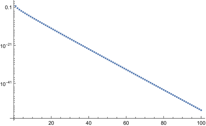
Figure 1: Log-plot of $f_{n}(q)$ for $q=0.2$. The horizontal axis is $n$.

One can extract $A(q)$ in (17) as the limit of the following sequence

$$A_{n}(q)=\sqrt{\frac{f_{n}(q)}{f_{n+1}(q)}}~{}~{}~{}\xrightarrow{n\to\infty}~{}~{}~{}A(q).$$ (18)

One can accelerate the convergence of the sequence by using the technique of the Richardson extrapolation, where the $m$-th Richardson transform of the series $A_{n}(q)$ is defined by

$$A_{n}^{(m)}(q)=\sum_{k=0}^{m}(-1)^{k+m}\frac{(n+k)^{m}}{k!(m-k)!}A_{n+k}(q).$$ (19)

It turns out that $A_{n}^{(m)}(q)$ has a much faster convergence to $A(q)$ than the original sequence $A_{n}(q)$. As an example, in Figure 2 we show the plot of $A_{n}(q)$ and its third Richardson transform $A_{n}^{(3)}(q)$ for $q=0.2$. As we can see from Figure 2, $A_{n}^{(3)}(q)$ converges to a constant much faster than the original $A_{n}(q)$.

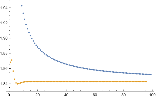
Figure 2: Plot of $A_{n}(q)$ (blue dots) and $A_{n}^{(3)}(q)$ (orange dots) for $q=0.2$. The horizontal axis is $n$.

We have computed $A(q)$ numerically for various values of $q$ using the $20$-th Richardson transform. See Figure 3 for the plot of $A(q)$ as a function of $q$.

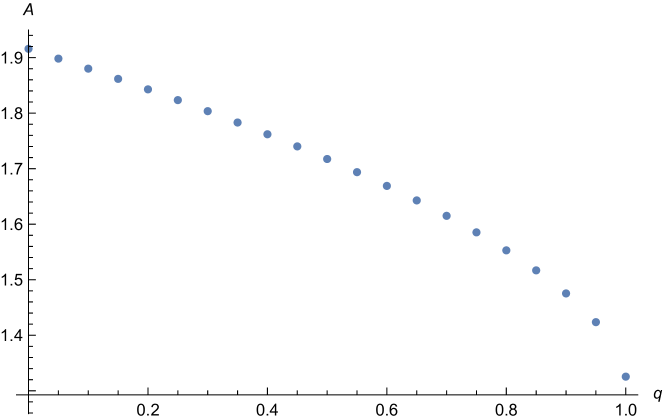
Figure 3: Plot of $A(q)$ as a function of $q$.

We can also determine $c(q)$ in (17) as the limit of the following sequence

$$c_{n}(q)=nf_{n}(q)\left[\frac{nf_{n}(q)}{(n+1)f_{n+1}(q)}\right]^{n}~{}~{}~{}\xrightarrow{n\to\infty}~{}~{}~{}c(q).$$ (20)

Again, using the technique of the Richardson extrapolation we can accelerate the convergence of $c_{n}(q)$ to $c(q)$. In this way, we find that $c(q)$ in (17) has a simple form

$$c(q)=1-q.$$ (21)

3 Interpretation of $A(q)$ as the first zero of $Z(\mathrm{i}t)$

When $0\leq q\leq 1$, the small $\beta$ expansion of the free energy (16) is an alternating series and the large $n$ asymptotics of $f_{n}(q)$ in (17) implies that this expansion is a convergent series with a finite radius of convergence

$$\log Z(\beta) \approx\sum_{n\geq 1}(-1)^{n-1}(1-q)^{n-1}\beta^{2n}\frac{1-q}{n}A(q)^{-2n}$$ (22)

$$=\log\Bigl{[}1+\beta^{2}(1-q)A(q)^{-2}\Bigr{]}.$$

The radius of convergence is determined by the logarithmic singularity of (22) at the imaginary value of $\beta$. If we define $\beta=\mathrm{i}t$, the singularity is located at $t=\pm t_{1}(q)$ with

$$t_{1}(q)=\frac{A(q)}{\sqrt{1-q}}.$$ (23)

As we will see below, this singularity corresponds to the first zero of the partition function.

For instance, let us consider the $q=0$ case. From the numerical analysis in the previous section, we find that $t_{1}(q)$ at $q=0$ is estimated as

$$t_{1}(0)=A(0)=1.915852985103756157807\cdots.$$ (24)

When $q=0$, the measure factor in (7) becomes a trigonometric function $(2\sin\theta)^{2}$, and the exact partition function is simply given by

$$Z(\beta)=\int_{0}^{\pi}\frac{d\theta}{2\pi}(2\sin\theta)^{2}e^{2\beta\cos\theta}=\frac{1}{\beta}I_{1}(2\beta),$$ (25)

where $I_{1}(z)$ denotes the modified Bessel function of the first kind. If we analytically continue $Z(\beta)$ to the pure imaginary $\beta=\mathrm{i}t$, the partition function becomes

$$Z(\mathrm{i}t)=\frac{1}{t}J_{1}(2t),$$ (26)

where $J_{1}(z)$ denotes the Bessel function.

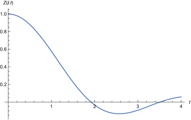
Figure 4: Plot of $Z(\mathrm{i}t)=\frac{1}{t}J_{1}(2t)$ for $q=0$.

See Figure 4 for the plot of $Z(\mathrm{i}t)$ in (26). $Z(\mathrm{i}t)$ in (26) has zeros along the real $t$-axis and the first zero on the positive $t$-axis is given by

$$t=\frac{1}{2}j_{1,1},$$ (27)

where $j_{n,k}$ is the $k$-th zero of the Bessel function $J_{n}(z)$. In Mathematica, $j_{n,k}$ is implemented as BesselJZero[n,k]. Using this function in Mathematica, the numerical value of (27) is evaluated as

$$\frac{1}{2}j_{1,1}=1.915852985103756157807\cdots,$$ (28)

which precisely matches (24)! In fact, we found more than 20-digit agreement between $\frac{1}{2}j_{1,1}$ and $t_{1}(0)=A(0)$ obtained from the Richardson extrapolation.

For general $q$, we do not know the closed form of the partition function $Z(\beta)$. However, one can easily evaluate $Z(\beta)$ numerically using the integral representation of $Z(\beta)$ in (7). As an example, in Figure 5 we show the plot of $Z(\mathrm{i}t)$ for $q=0.2$. We indicated the location of $t=t_{1}(q)$ by the vertical gray line. As one can see from Figure 5, $t=t_{1}(q)$ obtained from the Richardson extrapolation nicely agrees with the first zero of the partition function $Z(\mathrm{i}t)$. We have checked this agreement for several other values of $q$.

Figure 5: Plot of $Z(\mathrm{i}t)$ for $q=0.2$. The gray vertical line is at $t=t_{1}(q)$, which nicely agrees with the first zero of $Z(\mathrm{i}t)$.

From the above numerical evidence, it is natural to conjecture that the radius of convergence of the high temperature expansion of the free energy is equal to the first zero of the partition function $Z(\mathrm{i}t)$ along the positive real $t$ axis.

$t_{1}(q)$ in (23) diverges as $q\to 1$ due to the denominator $\sqrt{1-q}$, but $A(q)$ remains finite at $q=1$. From the Richardson extrapolation, we find

$$A(1)=1.32548683869836316194948\cdots.$$ (29)

We observe that this agrees with the maximal value of the function $f(s)=2s/\cosh s$

$$\max_{s\in\mathbb{R}}\left\{\frac{2s}{\cosh s}\right\}=1.32548683869836316194948\cdots.$$ (30)

The appearance of the function $f(s)=2s/\cosh s$ is expected from the semi-classical limit, as we will see in section 5.

In general, we expect that the partition function is written as an infinite product

$$Z(\beta)=\prod_{i=1}^{\infty}\left[1+\frac{\beta^{2}}{t_{i}(q)^{2}}\right],$$ (31)

where $t_{i}(q)$ is the $i$-th zero of $Z(\beta)$ along the imaginary $\beta$ axis. The first zero $t_{1}(q)$ is given by (23).

4 Padé approximation

Lets us go back to the real $\beta$ case. Using our data of $\{f_{n}(q)\}_{1\leq n\leq n_{\text{max}}}$ with $n_{\text{max}}=100$, we can improve the approximation of the small $\beta$ expansion in (16) by the (diagonal) Padé approximation

$$\log Z(\beta) \approx\sum_{n=1}^{n_{\text{max}}}(-1)^{n-1}(1-q)^{n-1}\beta^{2n}f_{n}(q)$$ (32)

$$\approx\frac{\sum_{i=0}^{n_{\text{max}}}b_{i}\beta^{i}}{\sum_{i=0}^{n_{\text{max}}}a_{i}\beta^{i}},$$

where the second line is the Padé approximant constructed in such a way that the small $\beta$ expansion of the second line agrees with the first line up to $\mathcal{O}(\beta^{2n_{\text{max}}})$. We can compare this Padé approximation with the exact result in (7). In Figure 6, we show the plot of free energy $\log Z(\beta)$ for $q=0.2$ in the Padé approximation (blue solid curve) and the exact result in (7) evaluated numerically (orange dots). As we can see from Figure 6, the Padé approximation of the small $\beta$ expansion exhibits a good agreement with the exact result even at large $\beta$.

This agreement suggests that there is no phase transition between the high temperature regime and the low temperature regime and they are smoothly connected. This is in contrast to the situation for the coupled SYK model considered in Maldacena:2018lmt where the high and the low temperature phases are separated by the Hawking-Page transition. Our result suggests that there is no Hawking-Page transition for the partition function $Z(\beta)$ of DSSYK.

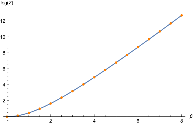
Figure 6: Plot of free energy $\log Z(\beta)$ for $q=0.2$. The blue solid curve represents the Padé approximation of the small $\beta$ expansion (32) with $n_{\text{max}}=100$, while the orange dots are the exact result in (7).

5 Semi-classical expansion

As discussed in Goel:2023svz , the $\theta$-integral in (7) can be evaluated by the saddle-point approximation in the semi-classical small $\lambda$ regime. To define the systematic small $\lambda$ expansion, we have to rescale $\beta\to\beta\lambda^{-\frac{1}{2}}$

$$Z(\beta\lambda^{-\frac{1}{2}})=\int_{0}^{\pi}\frac{d\theta}{2\pi}(q;q)_{\infty}(e^{2\mathrm{i}\theta};q)_{\infty}(e^{-2\mathrm{i}\theta};q)_{\infty}\exp\left(\frac{2\beta\cos\theta}{\sqrt{\lambda(1-q)}}\right).$$ (33)

As shown in Okuyama:2023bch , in the small $\lambda$ limit the measure factor is expanded as

$$(q;q)_{\infty}(e^{2\mathrm{i}\theta};q)_{\infty}(e^{-2\mathrm{i}\theta};q)_{\infty}=\sqrt{\frac{2\pi}{\lambda}}\exp\left[\frac{\lambda}{8}-\frac{2}{\lambda}\left(\theta-\frac{\pi}{2}\right)^{2}+\log(2\sin\theta)\right].$$ (34)

Note that there are no corrections higher than $\mathcal{O}(\lambda^{2})$ in the measure factor. Now, we can evaluate the $\theta$-integral by the saddle point approximation. At the leading order of the small $\lambda$ expansion, the saddle point equation is given by

$$\frac{\partial}{\partial\theta}\left[-2\left(\theta-\frac{\pi}{2}\right)^{2}+2\beta\cos\theta\right]=0,$$ (35)

and the saddle point value of $\theta$ is given by

$$\theta=\frac{\pi}{2}-u$$ (36)

where $u$ is related to $\beta$ as

$$\beta=\frac{2u}{\cos u}.$$ (37)

One can systematically improve the approximation by expanding the integrand around the saddle point

$$\theta=\frac{\pi}{2}-u+\sqrt{\lambda}x$$ (38)

and perform the Gaussian integral over the fluctuation $x$. In this way we find the semi-classical, small $\lambda$ expansion of the free energy

$$\log Z(\beta\lambda^{-\frac{1}{2}})=\sum_{k=0}^{\infty}\lambda^{k-1}\mathcal{F}_{k}(u).$$ (39)

The first few terms of $\mathcal{F}_{k}(u)$ read

$$\mathcal{F}_{0}(u) =-2u^{2}+4u\tan u,$$ (40)

$$\mathcal{F}_{1}(u) =u\tan u+\log(\cos u)-\frac{1}{2}\log(1+u\tan u),$$

$$\mathcal{F}_{2}(u) =\frac{4u^{4}\tan^{4}u+12u^{4}\tan^{2}u-12u^{3}\tan^{3}u+12u^{3}\tan u+5u^{2}-21u^{2}\tan^{2}u-5u\tan u}{96(u\tan u+1)^{3}},$$

$$\mathcal{F}_{3}(u) =\frac{1}{768(u\tan u+1)^{6}}\Bigl{[}-8u^{7}\tan^{7}u-16u^{7}\tan^{5}u-8u^{7}\tan^{3}u-24u^{6}\tan^{6}u$$

$$\quad-24u^{6}\tan^{4}u-42u^{5}\tan^{5}u-56u^{5}\tan^{3}u-6u^{5}\tan u+u^{4}-25u^{4}\tan^{4}u-56u^{4}\tan^{2}u$$

$$\quad+27u^{3}\tan^{3}u-15u^{3}\tan u-7u^{2}+33u^{2}\tan^{2}u+7u\tan u\Bigr{]}.$$

We are interested in the small $\beta$ regime, which corresponds to the small $u$ regime. The small $u$ expansion of $\mathcal{F}_{k}(u)$ in (40) is easily found as

$$\mathcal{F}_{0}(u) =2u^{2}+\frac{4u^{4}}{3}+\frac{8u^{6}}{15}+\frac{68u^{8}}{315}+\frac{248u^{10}}{2835}+\frac{5528u^{12}}{155925}+\frac{87376u^{14}}{6081075}+\frac{3718276u^{16}}{638512875}+\cdots,$$ (41)

$$\mathcal{F}_{1}(u) =\frac{u^{4}}{3}+\frac{2u^{6}}{45}+\frac{23u^{8}}{315}+\frac{34u^{10}}{14175}+\frac{8014u^{12}}{467775}-\frac{20236u^{14}}{8513505}+\frac{273653u^{16}}{58046625}+\cdots,$$

$$\mathcal{F}_{2}(u) =-\frac{u^{4}}{9}+\frac{2u^{6}}{9}-\frac{55u^{8}}{189}+\frac{2854u^{10}}{8505}-\frac{161786u^{12}}{467775}+\frac{6119348u^{14}}{18243225}-\frac{4744967u^{16}}{15324309}+\cdots,$$

$$\mathcal{F}_{3}(u) =\frac{u^{4}}{36}-\frac{17u^{6}}{90}+\frac{299u^{8}}{540}-\frac{19979u^{10}}{17010}+\frac{1900147u^{12}}{935550}-\frac{55729109u^{14}}{18243225}+\frac{31769442277u^{16}}{7662154500}+\cdots.$$

On the other hand, we can find the small $\lambda$ expansion of the free energy directly from (16)

$$\log Z(\beta\lambda^{-\frac{1}{2}}) =\sum_{n=0}^{\infty}(-1)^{n-1}\beta^{2n}\lambda^{-n}(1-q)^{n-1}f_{n}(q)$$ (42)

$$=\sum_{k=0}^{\infty}\lambda^{k-1}F_{k}(\beta).$$

Thanks to the presence of the factor $(1-q)^{n-1}$ in the expansion of free energy (16), one can take a well-defined semi-classical limit after rescaling $\beta\to\beta\lambda^{-\frac{1}{2}}$. The first few terms of $F_{k}(\beta)$ in (42) read

$$F_{0}(\beta) =\frac{\beta^{2}}{2}-\frac{\beta^{4}}{24}+\frac{\beta^{6}}{120}-\frac{23\beta^{8}}{10080}+\frac{67\beta^{10}}{90720}-\frac{5297\beta^{12}}{19958400}+\frac{997\beta^{14}}{9729720}-\frac{26618\beta^{16}}{638512875}+\cdots,$$ (43)

$$F_{1}(\beta) =\frac{\beta^{4}}{48}-\frac{7\beta^{6}}{720}+\frac{61\beta^{8}}{13440}-\frac{247\beta^{10}}{113400}+\frac{64091\beta^{12}}{59875200}-\frac{8849\beta^{14}}{16511040}+\frac{712196791\beta^{16}}{2615348736000}+\cdots,$$

$$F_{2}(\beta) =-\frac{\beta^{4}}{144}+\frac{\beta^{6}}{144}-\frac{43\beta^{8}}{8064}+\frac{289\beta^{10}}{77760}-\frac{590147\beta^{12}}{239500800}+\frac{822299\beta^{14}}{518918400}-\frac{156670559\beta^{16}}{156920924160}+\cdots,$$

$$F_{3}(\beta) =\frac{\beta^{4}}{576}-\frac{11\beta^{6}}{2880}+\frac{11\beta^{8}}{2304}-\frac{10417\beta^{10}}{2177280}+\frac{254201\beta^{12}}{59875200}-\frac{2170187\beta^{14}}{622702080}+\frac{21258243901\beta^{16}}{7846046208000}+\cdots.$$

The small $u$ expansion of $\beta$ in (37) is given by

$$\beta=\frac{2u}{\cos u}=2u\sum_{n=0}^{\infty}\frac{(-1)^{n}E_{2n}u^{2n}}{(2n)!},$$ (44)

where $E_{2n}$ denotes the Euler number. Plugging (44) into $F_{k}(\beta)$ in (43), we find that the small $u$ expansion of $F_{k}(\beta)$ agrees with $\mathcal{F}_{k}(u)$ in (41)

$$F_{k}\left(\frac{2u}{\cos u}\right)=\mathcal{F}_{k}(u).$$ (45)

To summarize, we find that the semi-classical small $\lambda$ expansion obtained from the saddle point approximation of the exact result is consistent with the small $\beta$ expansion of free energy in (16) after rescaling $\beta\to\beta\lambda^{-\frac{1}{2}}$. In other words, there is no order-of-limit problem between the small $\lambda$ expansion and the small $\beta$ expansion and we find the agreement of $\mathcal{F}_{k}(u)$ and $F_{k}(\beta)$ in (45).

Finally, we comment on the interpretation of $A(1)$ we found in section 3. The analytic continuation of $\beta$ to the imaginary value $\beta=\mathrm{i}t$ corresponds to the analytic continuation of $u$ to the imaginary value $u=\mathrm{i}s$. Then the relation (37) becomes

$$t=\frac{2s}{\cosh s}.$$ (46)

As we increase $t$ from zero, this relation ceases to have a solution above the maximum of the right hand side. Thus, it is natural that $A(1)=\max\{2s/\cosh s\}$ sets the value of the radius of convergence when $q=1$, if we regard the rescaled combination $\beta\sqrt{1-q}$ as the expansion parameter.

6 Conclusions and outlook

In this paper, we have studied the high temperature expansion of the free energy of DSSYK. We found that the radius of convergence of this expansion is determined by the first zero of the partition function along the imaginary $\beta$-axis. We have also computed the first few terms of the semi-classical expansion of free energy and found that they are consistent with the small $\beta$ expansion at finite $q$.

There are many interesting open questions. From the analysis of the Padé approximation of the small $\beta$ expansion and the numerical evaluation of the exact $Z(\beta)$ in (7), we find that there is no Hawking-Page transition for the partition function of DSSYK and the high and the low temperature regimes are smoothly connected. On the other hand, it is speculated that the UV completion of the SYK model involves stringy degrees of freedom Maldacena:2016hyu ; Goel:2021wim . Our result suggests that there is no Hagedorn growth of the degrees of freedom in DSSYK at high energy. In fact, the eigenvalue spectrum of the transfer matrix $T$ in (5) is bounded from above. It would be interesting to understand the stringy degrees of freedom in DSSYK better.

In general, we are still lacking a clear understanding of the bulk spacetime picture of DSSYK. In particular, we would like to understand the bulk dual of DSSYK at finite $\lambda$, away from the semi-classical limit. As discussed in Avdoshkin:2019trj , the moment $\langle 0|T^{2n}|0\rangle$ can be expanded as a sum over the Dyck paths and the limit shape of the Dyck paths are obtained for the case of the ordinary (not $q$-deformed) oscillators Avdoshkin:2019trj . It would be interesting to find the limit shape of the Dyck paths for the $q$-oscillator case, which might be related to the Brownian motion of the boundary particle discussed in Berkooz:2022mfk . We leave this as an interesting future problem.

- (1) S. Sachdev and J. Ye, “Gapless spin-fluid ground state in a random quantum heisenberg magnet,” Phys. Rev. Lett. 70 no. 21, (1993) 3339–3342, arXiv:cond-mat/9212030.
- (2) A. Kitaev, “A simple model of quantum holography (part 1),”. https://online.kitp.ucsb.edu/online/entangled15/kitaev/.
- (3) A. Kitaev, “A simple model of quantum holography (part 2),”. https://online.kitp.ucsb.edu/online/entangled15/kitaev2/.
- (4) J. Polchinski and V. Rosenhaus, “The Spectrum in the Sachdev-Ye-Kitaev Model,” JHEP 04 (2016) 001, arXiv:1601.06768 [hep-th].
- (5) J. Maldacena and D. Stanford, “Remarks on the Sachdev-Ye-Kitaev model,” Phys. Rev. D 94 no. 10, (2016) 106002, arXiv:1604.07818 [hep-th].
- (6) R. Jackiw, “Lower Dimensional Gravity,” Nucl. Phys. B252 (1985) 343–356.
- (7) C. Teitelboim, “Gravitation and Hamiltonian Structure in Two Space-Time Dimensions,” Phys. Lett. 126B (1983) 41–45.
- (8) J. S. Cotler, G. Gur-Ari, M. Hanada, J. Polchinski, P. Saad, S. H. Shenker, D. Stanford, A. Streicher, and M. Tezuka, “Black Holes and Random Matrices,” JHEP 05 (2017) 118, arXiv:1611.04650 [hep-th]. [Erratum: JHEP 09, 002 (2018)].
- (9) M. Berkooz, M. Isachenkov, V. Narovlansky, and G. Torrents, “Towards a full solution of the large N double-scaled SYK model,” JHEP 03 (2019) 079, arXiv:1811.02584 [hep-th].
- (10) A. Goel, V. Narovlansky, and H. Verlinde, “Semiclassical geometry in double-scaled SYK,” arXiv:2301.05732 [hep-th].
- (11) H. W. Lin, “The bulk Hilbert space of double scaled SYK,” JHEP 11 (2022) 060, arXiv:2208.07032 [hep-th].
- (12) M. Berkooz, M. Isachenkov, P. Narayan, and V. Narovlansky, “Quantum groups, non-commutative , and chords in the double-scaled SYK model,” arXiv:2212.13668 [hep-th].
- (13) K. Okuyama, “Hartle-Hawking wavefunction in double scaled SYK,” JHEP 03 (2023) 152, arXiv:2212.09213 [hep-th].
- (14) B. Mukhametzhanov, “Large p SYK from chord diagrams,” arXiv:2303.03474 [hep-th].
- (15) K. Okuyama and K. Suzuki, “Correlators of double scaled SYK at one-loop,” arXiv:2303.07552 [hep-th].
- (16) J. Touchard, “Sur Un Problème De Configurations Et Sur Les Fractions Continues,” Canadian Journal of Mathematics 4 (1952) 2–25.
- (17) J. Riordan, “The Distribution of Crossings of Chords Joining Pairs of Points on a Circle,” Mathematics of Computation 29 no. 129, (1975) 215–222.
- (18) M. Josuat-Vergés, “Cumulants of the -semicircular law, Tutte polynomials, and heaps,” Canadian Journal of Mathematics 65 no. 4, (2013) 863–878, arXiv:1203.3157 [math.CO].
- (19) M. Marino, R. Schiappa, and M. Weiss, “Nonperturbative Effects and the Large-Order Behavior of Matrix Models and Topological Strings,” Commun. Num. Theor. Phys. 2 (2008) 349–419, arXiv:0711.1954 [hep-th].
- (20) J. Maldacena and X.-L. Qi, “Eternal traversable wormhole,” arXiv:1804.00491 [hep-th].
- (21) A. Goel and H. Verlinde, “Towards a String Dual of SYK,” arXiv:2103.03187 [hep-th].
- (22) A. Avdoshkin and A. Dymarsky, “Euclidean operator growth and quantum chaos,” Phys. Rev. Res. 2 no. 4, (2020) 043234, arXiv:1911.09672 [cond-mat.stat-mech].