EP Aquarii: a new picture of the circumstellar envelope

Abstract

New analyses of earlier ALMA observations of oxygen-rich AGB star EP Aquarii are presented, which contribute major progress to our understanding of the morpho-kinematics of the circumstellar envelope (CSE). The birth of the equatorial density enhancement (EDE) is shown to occur very close to the star where evidence for rotation has been obtained. High Doppler velocity wings are seen to consist of two components, the front end of the global wind, reaching above $\pm$12 km s^-1, and an effective line broadening, confined within 200 mas from the centre of the star, reaching above $\pm$20 km s^-1 and interpreted as caused by the pattern of shock wfaves resulting from the interaction between stellar pulsation and convective cell granulation. Close to the star, episodic and lumpy mass ejections are observed, and their interaction with the gas of the nascent EDE, first rotating and later slowly expanding, is seen to play an important role in the development of the wind and the evolution of its radial velocity from 8-10 km s^-1 on the polar symmetry axis to $\sim$2 km s^-1 at the equator. It implies a very complex morpho-kinematics, which prevents making reliable interpretations with reasonable confidence. In particular, it sheds serious doubts on an earlier interpretation implying the presence of a white dwarf companion orbiting the star at an angular distance of $\sim$0.4 arcsec from its centre and currently west of it.

1 Introduction

When instruments providing observations of high sensitivity and angular and spectral resolutions became available, mainly the Very Large Telescope (VLT) and the Atacama Large Millimeter/submillimeter Array (ALMA), studies of the circumstellar envelopes (CSE) of Asymptotic Giant Branch (AGB) stars progressed rapidly. Yet, many questions are still unanswered concerning the mechanism that governs the generation and acceleration of the wind, in particular for oxygen-rich low mass-loss rate stars. In contrast with carbon-rich stars, these have a dusty envelope that is more transparent in the visible and near-IR, giving a better view of the innermost dust-forming atmospheric layers (Höfner & Freytag, 2019). Their study supports a scenario where the radiation pressure, which accelerates the outflows, is caused by photon scattering on highly transparent iron-free grains, such as corundum (Al₂O₃), which form a thin gravitationally bound dust layer close to the stellar photosphere; beyond it, silicate dust condenses on top of corundum cores, speeding up grain growth to the critical size.

Recent high-resolution imaging of nearby AGB stars at visible and infrared wavelengths has revealed complex, non-spherical distributions of gas and dust in the close circumstellar environment, with changes in morphology and grain sizes occurring over the course of weeks or months. At millimetre wavelengths complexity is the main feature that characterizes the morpho-kinematics of the CSE, with important anisotropy and inhomogeneity. Such distribution of atmospheric gas emerges naturally in 3-D hydrodynamical models (Höfner & Freytag, 2019) as a consequence of large-scale convective flows below the photosphere and the resulting network of atmospheric shock waves, the dynamical patterns in the gas being imprinted on the dust in the close stellar environment. Global AGB star models are characterized by giant convection cells, which can span over a steradian, and have a lifetime of many years. Together with radial pulsations, with typical periods at a few-month scale, they generate waves of various frequencies and spatial scales, which quickly develop into shock waves giving rise to ballistic gas motions peaking around 2 stellar radii. As the shock waves interact and merge, they produce large-scale regions of enhanced densities in their wakes.

A consequence of the resulting complexity is the difficulty to reconstruct reliably the observed morpho-kinematics of the CSE in both velocity and space, driving its study into proceeding somewhat by trials and errors: successive observations and analyses bring new information that helps refining the picture. EP Aquarii provides such an example with four recent publications by Homan et al. (2018), Tuan-Anh et al. (2019), Hoai et al. (2019) and Homan et al. (2020). It is an M-type, semi-regular variable star (spectral type M8III), with a pulsation period usually quoted as 55 days but more like 110$\pm$20 days (Eggen, 1973; Tabur et al., 2009), located at 119$\pm$6 pc from the solar system (van Leeuwen, 2007; Gaia Collaboration, 2018); it shows no technetium in its spectrum (Lebzelter & Hron, 1999) and has an effective temperature of $\sim$3240 K, a mass of $\sim$1.7 M_⊙, a radius of $\sim$0.77 au (Dumm & Schild, 1998) and a mass-loss rate of $\sim$(1.6$\pm$0.4) 10^-7 M_⊙yr^-1 (Hoai et al., 2019).

The resulting picture that emerges from the four more recent studies of the CSE is a two-component morpho-kinematics producing a Doppler velocity spectrum made of a narrow central peak at star systemic velocity and a broader plateau extending over $\sim\pm$10-11 km s^-1. The central peak is associated with an oblate, and the broad plateau with a prolate volume of gas, both expanding radially and sharing a same axis that projects $\sim$20^∘ west of north and is inclined by only $\sim$10^∘ with respect to the line of sight. The oblate volume of gas, referred to as Equatorial Density Enhancement (EDE), or occasionally torus or disc, is nearly face on, causing its radial expansion velocity to be poorly defined, $\sim$2 km s^-1. It hosts a complex pattern of arcs of enhanced CO(2-1) emission that is interpreted by Homan et al. (2018, 2020) in terms of a spiral produced by a white dwarf companion, with a mass of 0.65-0.80 M_⊙, orbiting EP Aqr at a distance of $\sim$0.4 arcsec and currently located west of it. The prolate volume of gas, usually referred to as polar or bi-conical outflows, displays maximal velocity along the line of poles but clear density depressions near the poles, the maximum being reached at stellar latitudes between $\sim\pm$45^∘ and $\sim\pm$60^∘ while the transition between oblate and prolate components occurs progressively near stellar latitudes of $\sim\pm$20^∘.

Evidence for rotation within some 100-200 mas from the centre of the star, with a rotation velocity at km s^-1 scale, has been obtained from the observation of the emissions of the CO(2-1), SO₂(16_6,10-17_5,13) and SO₂(4_2,2-3_1,3) lines (Homan et al., 2018, 2020; Tuan-Anh et al., 2019). Observations of the dust induced polarization of the 550-750 nm emission observed at the VLT using SPHERE-ZIMPOL (Homan et al., 2020) give evidence for a shell of dust surrounding the star and having an inner radius slightly smaller than 100 mas. A study of dust emission in the infrared using the Small Wavelength Spectrometer aboard ISO (Heras & Hony, 2005) has given evidence for very low ratios of both gas-to-dust mass and aluminium oxide to silicates relative abundance.

There exists no well-established interpretation of the observed morphology. EDE’s are usually described as the result of the gravitational attraction of the stellar wind in the orbital plane of a companion and the polar outflows are often interpreted as episodically produced by the rapid rotation of an accretion disc surrounding this companion and reach very high velocities. Such are the cases of HD 101584 (Olofsson et al., 2019) with highly collimated outflows reaching velocities of $\sim\pm$140 km s^-1, of $\pi^{1}$ Gruis (Doan et al., 2017, 2020; Homan et al., 2020) with polar outflows consisting of thin hourglass-shaped bubbles reaching a radial expansion velocity of $\sim$60 km s^-1, of V Hya (Sahai et al., 2022) with high velocity lumpy jets of velocity $\sim$175 km s^-1, and of R Aqr (Melnikov et al., 2018; Liimets et al., 2018; Bujarrabal et al., 2021) with outflows made of curved central jets with velocity reaching $\sim$240 km s^-1 surrounded by hourglass bubbles in ballistic expansion with velocity of $\sim$55 km s^-1. Much closer to the morpho-kinematics of the EP Aqr CSE is that of AGB star RS Cnc, which however displays a clear technetium signal, but is too boreal to be observed by ALMA and has been studied in detail using NOEMA (Winters et al., 2022). It has a two component morpho-kinematics, quantitatively similar to EP Aqr, with an axis making an angle of $\sim$30^∘ with the line of sight and radial expansion velocities reaching 3-4 km s^-1 in the EDE and 8-9 km s^-1 in the bipolar outflows.

Neither EP Aqr nor RS Cnc has been shown to host a companion (but in both cases the presence of an undetected companion cannot be excluded) and no other known AGB star displays a close enough morpho-kinematics to be claimed to serve as a model for their CSE. The question of their genesis remains therefore open and, in the case of EP Aqr, the picture proposed by Homan et al. (2020), suggesting the presence of an undetected white dwarf companion playing a major role in the formation and structure of the EDE, leaves several questions unanswered that call for further study:

i) High Doppler velocity wings, reaching $\sim\pm$20 km s^-1, were interpreted by Tuan-Anh et al. (2019) as two narrow polar structures, referred to as jets, launched from less than 25 au away from the star and building up between $\sim$20 au and $\sim$100 au to maximal velocity. However, subsequent analyses of similar high Doppler velocity wings observed in several other stars, as, for example $o$ Ceti (Hoai et al., 2020; Nhung et al., 2022), favoured interpretations in terms of shocks produced close to the star by pulsations and convective cells, shedding strong doubts on the jet interpretation proposed for EP Aqr. It has therefore become imperative to reconsider the case.

ii) The formation of the bipolar outflows remains unexplained. It may invite interpretations in terms of magnetic fields (García-Segura et al., 2005; Winters et al., 2022), or in terms of interacting winds in a binary (Nordhaus & Blackman, 2006; Castellanos-Ramírez et al., 2021), and more specifically in terms of an additional companion orbiting EP Aqr at a distance of $\sim$10 au (Homan et al., 2020), but none of these can be solidly justified. The latter authors present a number of relevant suggestive arguments in relation to the observation of a complex pattern of arcs in the emission of the polar outflows.

iii) The formation of the EDE remains equally unexplained. The interpretation proposed by Homan et al. (2020), in terms of focusing by an assumed white dwarf companion is in principle compelling but raises unanswered questions and is likely to face inconsistencies when details of the observed morpho-kinematics are being considered.

iv) A clear depression of SiO(5-4) line emission is observed in the western blue-shifted octant and interpreted by Homan et al. (2020) as the result of molecular dissociation produced by the UV radiation of the white dwarf companion. However, such dissociation should extend to the red-shifted hemisphere as well and the observed morphology of the depression is difficult to understand in such terms.

The aim of the present article is therefore to shed new light on these issues, by presenting new additional analyses of the emissions of the CO(2-1) and SiO(5-4) lines, in particular in the close neighbourhood of the star. As a brief reminder of the main properties of the CSE of EP Aquarii, we display in Figure 1 intensity maps of the CO(2-1) and SiO(5-4) line emissions, together with Doppler velocity spectra and a schematic description of the axi-symmetric geometry.

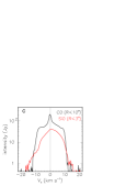
Figure 1: (a) intensity map of CO(2-1) emission; (b) intensity map of SiO(5-4) emission; (c) Doppler velocity spectra of both CO(2-1) and SiO(5-4) line emissions; (d) schematic of the red-shifts resulting from the tilted axi-symmetric geometry. The colour scales are in units of Jy arcsec^-2 km s^-1.

2 Observations and data reduction

We use archival ALMA observations of the CO(2-1) and SiO(5-4) line emissions of EP Aquarii that were performed in 2016 and 2019 under projects ADS/JAO.ALMA#2016.1.00057.S and ADS/JAO.ALMA#2018.1.00750.S, respectively (PI W. Homan). Observations and data reduction have been described in much detail by Homan et al. (2018, 2020) and do not need to be repeated here. The latter observations used an extended antenna configuration and were combined with the earlier observations of lower angular resolution. However, Homan et al. (2020) did not explicitly use the high angular resolution line data and based their analyses on the combined data. In the present article, we use instead the high angular resolution observations (referred to as TM0) explicitly to study the close neighbourhood of the star. Accordingly, we reduced these data and report about the results in the present section. As far as the combined data are concerned, it should be sufficient to summarize their main features in Table 1.

The 2019 observations were made in two steps, on June 5 and 14, respectively, with a hybrid antenna configuration (C43-10 and C43-9) including   46 antennas having baseline lengths between 83 and 16000 m. A gap at short spacing ($\sim$100-200 m), seen in the baseline length distribution of June 14 (Figure 2a), is due to the absence of four antennas (circled in red in Figure 2b). Four spectral windows were selected to observe line emissions of CO(2-1), SiO(5-4), SO₂(4_2,2-3_1,3), and ¹³CO(2-1). However, the latter two sets of data had insufficient sensitivity to contribute significantly new information and their analysis is omitted from the present work.

Table 1: Summary of Band 6 observations and data reduction of the CO(2-1) (230.55 GHz) and SiO(5-4) (217.12 GHz) line emissions.

Reference	Epoch	Line	Beam size (mas2)	Beam PA (∘)	Channel width (km s-1)	Time on source	Noise rms per channel (mJy beam-1)	Maximal recoverable scale (”)
Homan et al. (2018)	2016	CO(2-1) SiO(5-4)	170$\times$150	$-$34	$\sim$0.33	70 min (ACA) 230 min (TM1,2)	1.25	15
Combined data	2016,	CO(2-1)	87$\times$79	$+$15	$\sim$0.33	$-$	0.65	15
Homan et al. (2020)	2019	SiO(5-4)	85$\times$79	$+$7
TM0 data	2019	CO(2-1)	32$\times$28	$+$13	0.95	99 min	1.0	0.5
present work		SiO(5-4)	32$\times$30	$+$22	0.34		1.34	0.5

The data of June 5 and 14 observations of the CO(2-1) and SiO(5-4) line emissions have been merged with equal weights and grouped in frequency channels corresponding to Doppler velocity intervals of 0.95 and 0.34 km s^-1, respectively. Natural weighting was used for cleaning, producing maps of 2000$\times$2000 pixels covering $\pm$4 arcsec in both $x$ (pointing east) and $y$ (pointing north), with FWHM beam sizes of 31.7$\times$28.0 mas² and 32.4$\times$30.0 mas², respectively. We did not subtract the continuum contribution at visibility level, which would have been improper when looking over the stellar disc because of important absorption.

The impact of the lack of short spacing below $\sim$100 m was found to be different between the CO(2-1) line, with emission extending up to some 10 arcsec angular distance from the star and SiO(5-4) line emission, confined within some 3 arcsec. Moreover, in the case of the CO(2-1) line emission, it was also observed to be stronger near systemic Doppler velocity, where the emission is dominated by a disc extending to large angular distances. The size of the mask used in the cleaning procedure must therefore be chosen accordingly. We studied in detail images obtained with different mask sizes and retained a radius of 2 arcsec for the SiO(5-4) data and of 1 arcsec for the CO(2-1) data, resulting in noise levels of 1.34 mJy beam^-1 for SiO(5-4) line emission and 1.0 mJy beam^-1 for CO(2-1) line emission. While the nominal maximal recoverable scale (MRS) corresponding to the C43-10 antenna configuration is 0.46 arcsec, the impact on imaging of the lack of short spacing cannot be simply measured by a single number. As the angular distance from the star increases, it reduces the detected flux first uniformly, then introducing anisotropic distortions of the emission pattern. We studied its effect in much detail, both comparing the produced images with those given by the combined data and by modelling the source as discs of various sizes. While the decline of detected flux starts well below the nominal MRS, important distortions appear only beyond $\sim$0.6-0.7 arcsec. For the purpose of the present work, we checked carefully that whenever TM0 data were used, proper account was taken of this issue. Examples of comparison between TM0 and combined data are illustrated in Figures 2, 4, 14 and 15.

We use Cartesian coordinates with the $z$ axis pointing away from Earth in addition to the $x$ and $y$ axes in the plane of the sky. We refer the Doppler velocity $V_{z}$ to a systemic star velocity of $-$33.6 km s^-1 in conformity with earlier work, but its value is not known to better than a fraction of a km s^-1. We define an angular distance from the centre of the star as $R$=$\sqrt{x^{2}+y^{2}}$ and a position angle $\omega$ measured counter-clockwise from north.

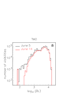
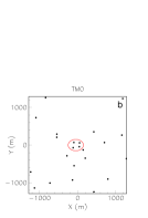
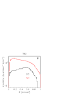
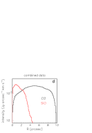
Figure 2: (a) distribution of the decimal logarithm of the uv distance (in meters) for the different data sets; (b) antenna configuration (centre region); the four antennas circled in red were absent for the June 14 observations; (c,d) radial distributions of CO (black) and SiO (red) emissions using TM0 (c) and combined data (d).

3 Equatorial density enhancement

3.1 CO(2-1) emission

Evidence for the presence of an equatorial density enhancement (EDE) is known from previous work to rest on the observation of the CO(2-1) and CO(1-0) line emissions exclusively (Hoai et al., 2019). However, a clear distinction between EDE and polar outflows could only be made at distances from the star exceeding $\sim$2 arcsec. The availability of high angular resolution data makes it now possible to study the EDE morphology at short distances from the star. As illustrated in the upper panels of Figure 3, Doppler velocity spectra integrated over successive rings centred on the star give clear evidence for the presence of the narrow component when $R$ exceeds $\sim$200 mas. It covers Doppler velocities between 0 and +2 km s^-1. Remarkably, the neighbouring channels, between $-$3 and 0 km s^-1 and 2 and 5 km s^-1, respectively, are depopulated. This suggests that below some 200 mas from the centre of the star, gas is focused toward the equatorial plane. Channel maps integrated over the corresponding intervals of Doppler velocity are displayed in the lower panels of Figure 3. In the depopulated Doppler velocity intervals ($-$3 to 0 and 2 to 5 km s^-1), we note enhancements of emission in the NE direction of the blue-shifted hemisphere and SW direction of the red-shifted hemisphere, which suggest being caused by rotation. In contrast, in the intervals of high $|V_{z}|$ values ($-$10 to $-$3 and 5 to 12 km s^-1), we see enhancements of emission in the NW direction of the blue-shifted hemisphere and SE direction of the red-shifted hemisphere, which suggest being caused by the effect on expansion of the inclination of the axisymmetry axis with respect to the line of sight.

In order to better explore the morpho-kinematics of the nascent EDE, we display in Figure 4 $V_{z}$ vs $\omega$ maps of the CO(2-1) emission in 100 mas wide rings centred on the star. They show that the EDE is already present in the smaller ring, $R$ between 100 and 200 mas, and its kinematics is dominated by rotation at a few km s^-1 scale. This evidence for very precocious formation of the EDE is an important observation that had not been made earlier. In particular, it conflicts with the interpretation given by Homan et al. (2020), which would imply an inner EDE radius of $\sim$400 mas, corresponding to the orbit of the assumed companion, with strong anisotropy. Unfortunately, with presently available data, it is difficult to take apart, in the immediate neighbourhood of the star, say below $R$$\sim$200 mas, the contributions of expansion, of rotation and of phenomena related to the generation of the nascent wind: dust formation and shock waves caused by the interaction between stellar pulsation and convective cell granulation (see Section 5).

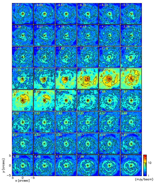
Figure 23: Channel maps of CO(2-1) emission (combined data). Central Doppler velocities (km s^-1) are indicated for each channel on the upper-left corner of the panel.

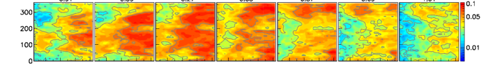
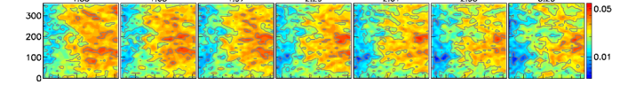
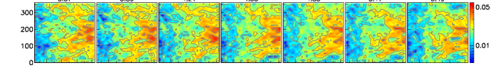
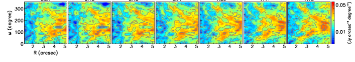
Figure 24: Channel maps of CO(2-1) emission (combined data) in the $\omega$ vs $R$ plane. Central Doppler velocities (km s^-1) are indicated for each channel on top of the panel.

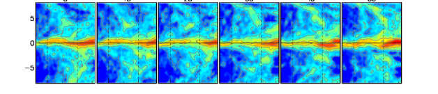
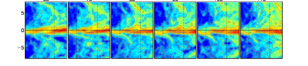
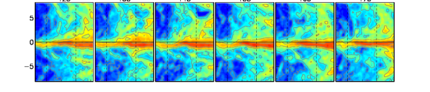
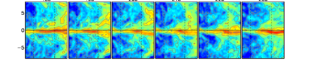
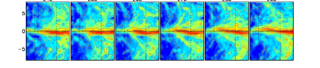
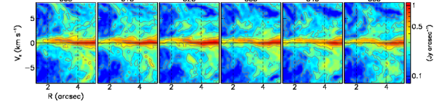
Figure 25: Projections of the data cube of CO(2-1) emission (combined data) in 36 intervals of $\omega$ (the central value in degree is indicated on top of each panel) on the $V_{z}$ vs $R$ plane ($|V_{z}|$$<$8 km s^-1, 1.2$<$$R$$<$5.2 arcsec).

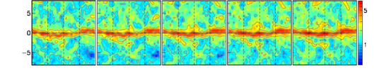
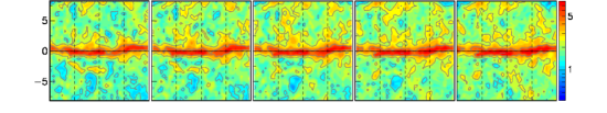
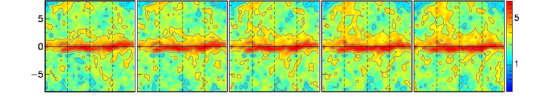
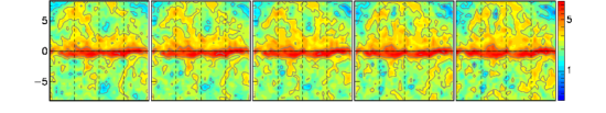
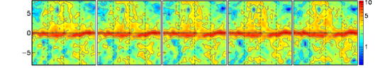
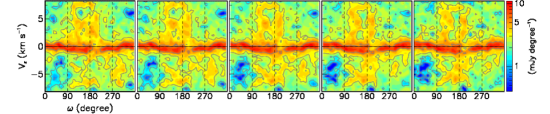
Figure 26: Projections of the data cube of CO(2-1) emission (combined data) in 40 intervals of $R$ (the central value in arcsec is indicated on top of each panel) on the $V_{z}$ vs $\omega$ plane ($|V_{z}|$$<$8 km s^-1, 0$<$$\omega$$<$360^∘).

Farther away from the star, the EDE is seen to subsist up to large distances, as illustrated in the pair of left panels of Figure 5 by the PV maps of the line emission seen in the ring 1.2$<$$R$$<$5.2 arcsec (see also channel maps of the CO(2-1) emission shown in Appendix in both the $x$ vs $y$ plane, Figure 23, and the $\omega$ vs $R$ plane, Figure 24). These maps, drawn in the $V_{z}$ vs $R$ and $V_{z}$ vs $\omega$ planes, respectively, show enhanced emission over all values of $R$ and $\omega$ in the central Doppler velocity interval, $|V_{z}|$$<$2 km s^-1. Similar PV maps drawn in small intervals of $R$ and $\omega$ are shown in Appendix (Figures 25 and 26). In each ($\omega,R$) bin, with a width of 10^∘$\times$100 mas, we calculate the mean and rms values of $V_{z}$ over the central Doppler velocity interval, $|V_{z}|$$<$2 km s^-1. Their values are shown as a function of $R$ and $\omega$ in the pair of right panels of Figure 5. They display remarkable uniformity, the rms value staying near 1 km s^-1 over the whole radial range and the mean value near zero. A small $\omega$ asymmetry of the latter, below $R$$\sim$3 arcsec, reveals an inclination of the EDE with respect to the plane of the sky consistent with the known inclination of the axis of the CSE with respect to the line of sight: it reaches values of $\sim$0.3 km s^-1 in the NW direction and of $\sim$$-$0.3 km s^-1 in the SE direction. This suggests a radial expansion velocity at the scale of $\sim$0.3/sin10^∘=1.7 km s^-1, consistent with the low value of 1.9 km s^-1 retained in earlier studies (Hoai et al., 2019). The rms deviation of 1 km s^-1 combines the effect of the known rms flaring angle of $\sim$15^∘, sin15^∘$\times$1.7=0.44 km s^-1 to an intrinsic width of $\sim$0.9 km s^-1.

Figure 3: CO(2-1) line emission, TM0 data. Upper panels: Doppler velocity spectra in successive rings, each 100 mas wide, starting from the circle of radius 100 mas centred on the star. Lower panels: brightness maps averaged over the velocity intervals associated with the structure of the spectra displayed on the upper panels for $R$$>$200 mas, and indicated on top of each panel.

Figure 4: CO(2-1) emission: TM0 (upper row) and combined (lower row) data. $V_{z}$ vs $\omega$ maps in 100 mas wide rings as indicated on top of each panel. The vertical lines are at $\omega$ values of 180, 270 and 360^∘. The sine waves shown as reference correspond to pure rotation with a velocity of 4 km s^-1. Pure expansion of a same velocity would be phase-shifted by $+$90^∘. The colour scales are in units of mJy beam^-1.

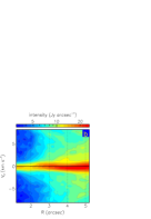
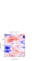
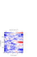
Figure 5: CO(2-1) line emission, combined data. Left pair of panels: PV maps in the $V_{z}$ vs $\omega$ (panel a) and $V_{z}$ vs $R$ (panel b) planes of the projections of the data cube defined as 1.2$<$$R$$<$5.2 arcsec and $|V_{z}|$$<$8 km s^-1. Right pair of panels: distribution in the $\omega$ vs $R$ plane of the mean (panel c) and rms (panel d) values of $V_{z}$ over the central Doppler velocity interval, $|V_{z}|$$<$2 km s^-1.

3.2 SiO(5-4) emission

In order to compare CO(2-1) and SiO(5-4) line emissions in the close neighbourhood of the star, we display in Figure 6 for SiO(5-4) (TM0 data) the same distributions as shown in Figure 3 for CO(2-1). They show a very different picture than those of CO(2-1) emission. The spectra cover a broad range of Doppler velocities, independently from the distance to the star, with no sign of change beyond 200 mas. The narrow component contributes only a very small enhancement. Absorption from the outer layer having reached terminal velocity at 8-10 km s^-1 is seen on all four spectra. In contrast with CO(2-1) emission, the brightness maps show little structure but reveal the presence of a strong depression of emission at $\sim$400 mas west from the centre of the star. This depression has been abundantly studied and commented upon in the earlier literature and we report on its properties in Section 4, to which we defer possible interpretations. Here we simply remark that the different response to temperature of the two lines can only have small effects. They differ essentially by the value of the energy $E_{\text{up}}$ of the upper level, 16.60 K for CO(2-1) and 31.26 K for SiO(5-4). This quantity enters in the expression of the emissivity as a factor e${}^{-E_{\text{up}}/T}$, where $T$ is the temperature. The ratio between CO(2-1) and SiO(5-4) line emissions of the values taken by this factor for $T$=10 K, 20 K, 50 K and $>$100 K is 4.3, 2.1, 1.3 and $<$1.2, respectively.

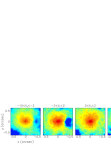
Figure 6: Same as Figure 3 for the SiO(5-4) emission.

3.3 Patterns of enhanced CO(2-1) emission

The emission of the CO(2-1) line is known from earlier work to display significant fluctuations. Hoai et al. (2019) remarked that both CO(1-0) and CO(2-1) emissions in the EDE display remarkably similar intensity fluctuations, at the level of $\sim\pm$36%, dominated by an eastern enhancement in the form of an arc and a southwestern depression, together having the appearance of a spiral. Homan et al. (2018) described similar data as evidence for a bright nearly face-on spiral structure, claiming the first convincing detection of a spiral in the circumstellar environment of an oxygen-rich AGB star, with a higher degree of small scale hydrodynamical structure and wider spiral arms than in carbon-rich environments. In their second paper, Homan et al. (2020) gave a very detailed description of the EDE intensity fluctuations and concluded that the observed complex emission pattern strongly resembles the typical hydrodynamical gas flow patterns associated with the interaction of a mass-losing AGB star with a companion. They claimed to have identified the flow along the L1 and L3 Lagrange points, before they coalesce into the spiral that manifests at larger length-scales and argued for the presence of a companion located at 0.4 arcsec to the west of the star, probably a white dwarf, with a mass between 0.65 and 0.8 M_⊙.

Channel maps of the combined data of CO(2-1) line emission in the twelve frequency channels that bracket the systemic velocity of the star ($-$2.0$<$$V_{z}$$<$1.8 km s^-1) are shown in Figure 7. They display arcs of enhanced emission. The complexity of the patterns makes a reliable interpretation in terms of well identified individual components difficult. In particular it makes it easy to interpret two partly overlapping arcs as a single one and an arc that is not centred on the star as a spiral arm. The human eye is too subjective a tool for a reliable interpretation of the observed patterns. In particular, the reality of the spiral discovered by Homan et al. (2018) deserves being critically discussed. There is no doubt that identifying such a spiral in the pair of central frequency channels (centred at 0.05 and $-$0.27 km s^-1, Figure 7) is a natural and reasonable thing to do. However, we note that the neighbouring channels (centred at 0.37 and $-$0.59 km s^-1, respectively) host patterns suggesting that the source of emission is in a plane inclined with respect to the sky plane: they shine in the NW direction for the red-shifted side and in the SE direction for the blue-shifted side, as expected for a plane perpendicular to the known axis of the CSE. Correcting for this tilt by averaging the brightness over the four central channels, ($-$0.75$<$$V_{z}$$<$0.53 km s^-1) we obtain the map shown in the left panel of Figure 8. The identification of a spiral as proposed by Homan et al. (2018) and shown in the central panel of the figure is no longer obvious. Assessing the reliability of the identification of such a spiral is indeed difficult. As illustrated in the right panel of Figure 8, arcs of spirals are excellent approximations to arcs of circles having their centre offset with respect to the centre of the star. But the two halves of a single circle correspond to different spirals winding in opposite directions, a proper spiral winding instead in a single direction and expanding indefinitely: an arc having a point of closest approach to the star cannot be described as a single spiral.

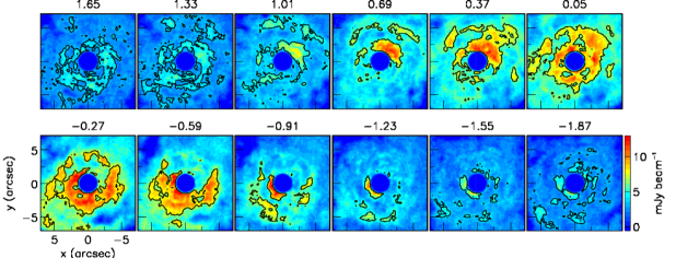
Figure 7: Channel maps of the CO(2-1) line emission (combined data) over the Doppler velocities (km s^-1) covering the EDE ($|V_{z}|$$<$$\sim$2 km s^-1) as indicated on top of each panel. The central region ($R$$<$1 arcsec) is excluded. Contours are shown at 50% of the maximal brightness.

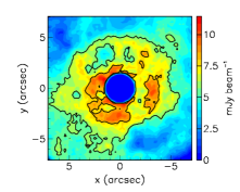
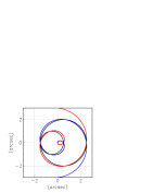
Figure 8: Left: Brightness of the CO(2-1) line emission (combined data) averaged over the four central panels of Figure 7 ($-$0.75$<$$V_{z}$$<$0.53 km s^-1). Contours are shown at 50% and 70% of maximal brightness. Centre: from Figure 5 of Homan et al. (2018), central channel of the CO(2-1) line emission. A black dashed Archimedean spiral is over plotted to guide the eye. Right: Comparing two spirals of equation $\rho=0.5+\alpha/\pi$ (blue and red) with two circles (black) of radius $R=1$ (2) offset by $-$0.5 (+0.5) with respect to the origin. The polar angle $\alpha$ cancels on the axis along which the circles are offset and increases clockwise for the blue spiral and counter-clockwise for the red spiral.

4 Polar outflows

4.1 CO(2-1) emission

The polar outflows cover a broad region of the sky up to large velocities. This is illustrated in Figure 9, which displays radial distributions of the CO(2-1) emission in selected intervals of Doppler velocity. In the red-shifted hemisphere, the distributions are apparently made of two components: the first of these extends up to $\sim$10 arcsec independently from the Doppler velocity interval; the second is narrower, with a full width increasing with $V_{z}$ from $\sim$1 arcsec at $V_{z}\sim 2$ km s^-1 to $\sim$4 arcsec at $V_{z}\sim 8$ km s^-1, its mean value decreasing from nearly 7 arcsec to $\sim$4 arcsec. Such morphology corresponds to the polar density depression described by Hoai et al. (2019) and to the appellation of “bi-conical” outflows used by Homan et al. (2020). As was noted earlier, the blue-shifted outflow shows less clear a structure, even if qualitatively similar to the red-shifted one. A simplified schematic of the morpho-kinematics of the CSE is shown in the right panel of Figure 9.

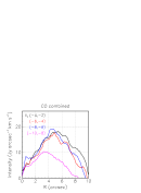
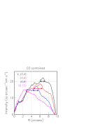
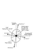
Figure 9: Left pair of panels: radial distributions of the CO(2-1) emission (combined data) integrated over position angle and over Doppler velocity intervals as indicated in the inserts. The double arrows in the central panel show the enhancement causing the apparently bi-conical structure. Right panel: schematic drawing of the geometry.

The polar outflows were observed earlier to display density fluctuations at the level of $\sim$$\pm$26%, and to reveal both an asymmetry between blue and red sides and significant differences between CO(1-0) and CO(2-1) emissions (Hoai et al., 2019). The higher angular resolution of the present data allows for an improved study of the morphology of the enhancements of CO(2-1) line emission. We studied in great detail the data cube (combined data) covering 51 frequency channels (Doppler velocities between $-$8.2 and $+$8.2 km s^-1) and projected angular distances from the star between 1.2 and 5.2 arcsec (Figures 23 to 26 of the Appendix). On occasions, with the aim of improving the identification of patterns of enhanced emission, we examined the brightness divided by a power fit to its radial distribution in the relevant frequency channel of the form $AR^{b}$. Values of $b$ for each frequency channel are displayed in the left panel of Figure 10. On average, $b=-0.29\pm 0.09$.

Ideally, one would like to describe each channel map as a set of well-identified separated arcs of enhanced emission. We attempted to do so by using an algorithm lumping together the brighter pixels. But we failed to obtain a satisfactory result, the complexity of the patterns preventing reliable pattern recognition. Instead, for each frequency channel, we inspected carefully the different projections of the data cube and tried to describe the observed patterns as simply and reliably as possible. Both ($x,y$) and ($R,\omega$) maps turned out to be useful. On the latter, concentric circles would show up as lines parallel to the ordinate ($\omega$) axis. But they show instead oblique lines, which would correspond to spirals. However, we remarked that such oblique lines were often associated with lines of opposite slopes, suggesting that instead of spirals, we observe eccentric circles. Figure 10 displays a pair of representative examples; they have not been selected to show particularly clear patterns. There are many examples of clearer cases as well as of more obscure cases.

Rather than giving a detailed review of our observations, we simply list the main statements which we can make with confidence: in each map, the pattern of enhanced emission can be described as a set of arcs; they are too numerous, frequently overlapping, to allow for reliable pattern recognition; they can be approximated by arcs of circles covering a few tens of degrees, typically less than 180^∘; the contrast is small, with a peak-to-valley ratio not exceding a factor 2; the arcs always wind around the star, implying that the centre of the associated circle is offset by less than a radius, typically half a radius, from the centre of the star; their radii cover a broad range of values, from as small as permitted by the angular resolution to as large as permitted by the size of the maps under study, namely from a fraction of an arcsecond up to over 5 arcsec; very similar patterns are observed in adjacent frequency channels, covering ranges up to a few km s^-1.

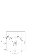
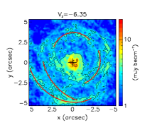
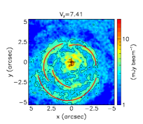
Figure 10: Left: best fit value of the power $b$ of fits of the form $AR^{b}$ to the radial brightness distribution, integrated over position angle and over the range 1.2$<$$R$$<$5.2 arcsec, as a function of Doppler velocity. The pair of right panels shows examples of patterns of enhanced emission in the blue-shifted (left) and red-shifted (right) hemispheres. Lines guide the eye on some arbitrarily selected patterns.

Finally, we remark that the $V_{z}$ vs $R$ map shown in Figure 5b (see also Figure 25 of the Appendix) provides precious information on the dependence of the radial expansion velocity on stellar latitude $\alpha$. It was assumed to be of the form $V=V_{\text{eq}}+(V_{\text{pole}}-V_{\text{eq}})\times\sin^{2}{\alpha}$ in Hoai et al. (2019), where $V_{\text{eq}}$ and $V_{\text{pole}}$ are the expansion velocities at equator and pole, respectively. As illustrated in Figure 11, a small volume of gas at distance $r$ from the star, at latitude $\alpha$ and having a radial velocity $V$ has coordinates $V_{z}=V\sin{\alpha}$ and $R=r\cos{\alpha}$. Namely a spherical shell expanding at radial velocity $V_{0}$ and observed when it reaches a radius $R_{0}$, is seen as a circle of unit radius in the PV map $V_{z}/V_{0}$ vs $R/R_{0}$. In contrast, a ring expanding at the equator at velocity $V_{1}$ is seen as a point on the $R$ axis at $V_{1}/V_{0}$. Understanding the transition between the polar outflows and the EDE implies understanding the transition between these two regimes. Namely, a shell emitted at some time with velocity $V_{0}$ at the pole and velocity $V_{1}$ at the equator is seen as a curve of equation $V/V_{0}=V_{1}/V_{0}+(1-V_{1}/V_{0})f(\vartheta)$ where $\vartheta$ is the polar angle, with $f$(0)=0 and $f$(90^∘)=1. But $\vartheta$ is equal to the stellar latitude $\alpha$ because the reference radius $R_{0}$ used to define the axis of abscissa is the distance covered at velocity $V_{0}$, used as reference velocity on the axis of ordinate. Namely the curve representing the shell in the PV diagram is a direct representation of the function $f(\alpha)$ that describes the dependence on stellar latitude of the expansion velocity. The left panel of Figure 11 shows three examples of function $f(\alpha)$, all three of the form sin${}^{n}\alpha$, with $n=\frac{1}{2}$, 1 and 2 respectively (in addition to the trivial cases $f(\alpha)$=0 and 1). Comparison with low latitude observations, as shown in the right panels of Figure 11 (see also Figure S3), favours clearly values of $n$ smaller than 1, in contradiction with the arbitrary assumption made in Hoai et al. (2019). This is important information for modelling the hydrodynamical flow, however a task beyond the scope of the present work.

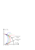
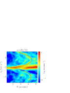
Figure 11: Latitudinal dependence of the radial expansion velocity. Left: schematics. Centre and right : two examples of $V_{z}$ vs $R$ maps (CO(2-1) combined data) at $\omega$=65^∘ and 205^∘, respectively (from Figure S3).

4.2 SiO(5-4) emission: general features

In contrast to CO(2-1) emission, SiO(5-4) emission is confined within radial distances of $\sim$3 arcsec, as shown in Figure 12, which displays radial distributions using the same format as for CO(2-1) emission in the left panels of Figure 9. The emissions of the two lines are indeed expected to differ in several respects: the SiO emission decreases with distance to the star, both because of condensation on dust grains and of dissociation by UV interstellar radiation; moreover, it is an efficient shock tracer. As a result, understanding the dynamics underlying the morpho-kinematics of both CO(2-1) and SiO(5-4) emissions is very challenging.

As already remarked, and clearly apparent on the distributions of SiO(5-4) emission displayed in Figure 13, one observes a significant asymmetry between the blue-shifted and red-shifted hemispheres. In particular the former reveals the presence of a strong depression of emission at some 400 to 500 mas west of the centre of the star that is challenging interpretation. In a first step, we limit therefore our considerations to the morphokinematics of the red hemisphere. To illustrate the inhomogeneity of the data cube, we show in Figure 13 the radial distribution $U(R)$, averaged over position angle and integrated over $V_{z}$, and the Doppler velocity spectrum $S(V_{z})$, of the volume of the data cube defined as 0.5$<$$R$$<$2.3 arcsec, 0$<$$V_{z}$$<$8 km s^-1; we then compare the observed intensity to the product $U(R)\times S(V_{z})$, properly normalized, in the right panels of the same figure. At the same time as the result reveals clearly the morpho-kinematics of the observed deviations with respect to a smooth distribution, it shows that their amplitude is relatively modest, typically at the level of $\pm$20%. Both $U(R)$ and $S(V_{z})$ show no significant fluctuation and the lumps of enhanced emissions have typical sizes at the scale of a fraction of an arcsec. In contrast, on the $V_{z}$ vs $R$ and $V_{z}$ vs $\omega$ maps, they cover several km s^-1.

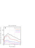
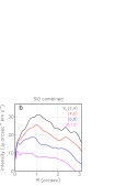
Figure 12: Radial distributions (combined data), shown separately in the blue-shifted and red-shifted hemispheres, for the SiO(5-4) emission (a and b) and CO(2-1) emission (c and d) integrated over position angle and over Doppler velocity intervals as indicated in the inserts.

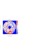
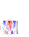
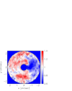
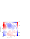
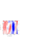
Figure 13: SiO(5-4) emission (combined data) in the red-shifted (upper row) and blue-shifted (lower row) hemispheres and the radial interval 0.5$<$$R$$<$2.3 arcsec. From left to right: Doppler velocity spectrum, $S(V_{z})$; radial distribution, $U(R)$; ratio of the observed intensity to $U(R)\times S(V_{z})$, properly normalized, in the $x$ vs $y$, $V_{z}$ vs $R$ and $V_{z}$ vs $\omega$ planes, respectively.

Repeating the same analysis for the blue-shifted hemisphere, we obtain the result illustrated in the lower row of Figure 13. The main difference with the red-shifted hemisphere is a lower intensity, by $\sim$33%, dominated by an important depression in the western quadrant causing a deviation twice as large with respect to the smooth distribution. If it were not for this depression, in the approximation of neglecting fluctuations at the level of $\pm$20%, both hemispheres would reveal similar morpho-kinematics, which could be described by a simple model. It is therefore important to study it in detail, which we do in the following sub-section.

Channel maps of the SiO(5-4) line emission are shown as supplementary material (Figure S1). Also shown are PV maps in the $V_{z}$ vs $R$ plane (Figure S2) and in the $V_{z}$ vs $\omega$ plane (Figure S3), which display episodic and lumpy emission.

4.3 SiO(5-4) emission in the close neighbourhood of the star

Qualitatively, the upper and lower rows of Figure 13 display some similarities: below $R$$\sim$1 arcsec, they both show enhanced emission in the polar outflows, at $V_{z}$$\sim$7 and $-$5 km s^-1, respectively, the former south, the latter north. In contrast, beyond $R$$\sim$1 arcsec, emission is enhanced near the EDE.

Figure 14 displays $V_{z}$ vs $\omega$ maps of SiO(5-4) emission in 100 mas wide rings centred on the star, in the same format as was shown for CO(2-1) emission in Figure 4. Very close to the star, for 100$<$$R$$<$200 mas, there are two very broad outflows of SiO(5-4) emission, one covering the whole southern hemisphere with $V_{z}$ between $\sim$4 and 12 km s^-1 and the other covering the whole northern hemisphere with $V_{z}$ between $\sim$$-$6 and $+$1 km s^-1. When $R$ increases, the emissions of both outflows cover narrower intervals of position angles and important depressions of emission appear: a northern red-shifted void in the $R$$\sim$200 mas range and, later, a western blue-shifted void in the $R$$\sim$400 mas range (see also the spectra displayed in Figure S4 of the supplementary material).

While qualitative similarities between both outflows and associated voids are remarkable, as clearly illustrated in Figure 15, important differences must be noted: i) the western blue-shifted depression of SiO(5-4) emission is stronger than the northern red-shifted one, with a peak-to-valley ratio of $\sim$6 compared with $\sim$3; ii) the northern SiO(5-4) depression starts earlier than the western one and is already present in the interval 0.1$<$$R$$<$0.2 arcsec where the western depression is not only absent but even partly replaced by a clear enhancement; iii) the southern outflow, covering large Doppler velocities, is emitted in the red-shifted hemisphere close to the line of sight while the northern outflow, covering small Doppler velocities, must interact with the nascent EDE in the equatorial plane. Indeed, Figure 16 shows that the CO(2-1) emission of the EDE displays a western void of emission clearly associated with the edge of the blue-shifted void of SiO(5-4) emission.

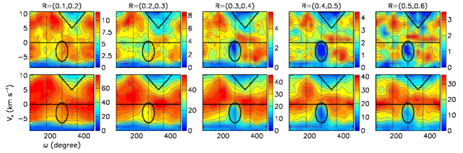
Figure 14: SiO(5-4) TM0 (upper row) and combined (lower row) data. $V_{z}$ vs $\omega$ maps in 100 mas wide rings as indicated on top of each panel. A triangle and an ellipse, corresponding approximately to the location of the voids of emission, are shown as reference in all panels. The colour scale is in mJy beam^-1.

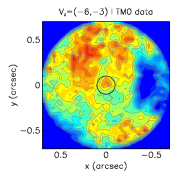
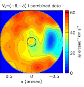
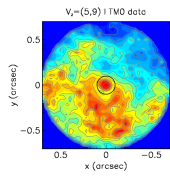
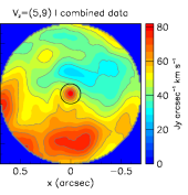
Figure 15: SiO(5-4) intensity maps integrated over $-$6$<$$V_{z}$$<$$-$3 km s^-1 for the left pair of panels and over 5$<$$V_{z}$$<$9 km s^-1 for the right pair of panels. The intensity is multiplied by $R$/0.1 for $R$$>$0.1 arcsec. In each pair, TM0 data are shown left and combined data are shown right.

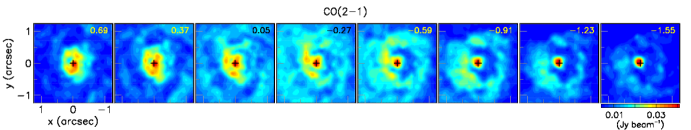
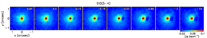
Figure 16: EDE region, combined data. CO(2-1) (upper row) and SiO(5-4) (lower row) emissions: channel maps centred at the Doppler velocities indicated on top of each panel.

These observations underscore the complexity of the dynamics at stake and suggest that the interaction between the northern outflow and the nascent EDE may play an important role. Particularly puzzling are the properties displayed by the blue-shifted western void of SiO(5-4) emission. In order to explore it in more detail, we define a volume $\Omega_{\text{void}}$ of the data cube, meant to cover it, as 0.25$<$$R$$<$1 arcsec, 240^∘$<$$\omega$$<$300^∘ and $-$6$<$$V_{z}$$<$$-$2 km s^-1. We then release one or two of the constraints associated with these inequalities and study the distribution of the brightness in the region that has been made free of the constraint. The result is displayed in Figure 17 for both SiO(5-4) and CO(2-1) emissions (combined data) and for their ratio.

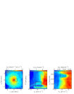
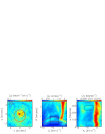
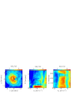
Figure 17: Western depression (combined data) as seen by SiO(5-4) (upper row), CO(2-1) (middle row) and their ratio (lower row). From left to right: $x$ vs $y$ map for $-$6$<$$V_{z}$$<$$-$2 km s^-1; $R$ vs $V_{z}$ map for 240$<$$\omega$$<$300^∘; $\omega$ vs $V_{z}$ map for 0.25$<$$R$$<$1 arcsec; $R$ distribution for $-$6$<$$V_{z}$$<$$-$2 km s^-1, 240$<$$\omega$$<$300^∘; $\omega$ distribution for $-$6$<$$V_{z}$$<$$-$2 km s^-1, 0.25$<$$R$$<$1 arcsec; $V_{z}$ distribution for 240$<$$\omega$$<$300^∘, 0.25$<$$R$$<$1 arcsec. The black lines on the maps and the double arrows on the histograms show the limits used to define $\Omega_{\text{void}}$. In the pair of left most panels, the red lines show small enhancements of emission suggested in the text.

Globally ($x$ vs $y$ maps and $\omega$ distributions of Figure 17), CO emission is slightly enhanced and SiO emission strongly depressed in $\Omega_{\text{void}}$. As seen in the $\omega$ vs $V_{z}$ maps of Figure 17, the enhancement of CO emission, in the interval 0.25$<$$R$$<$1 arcsec, covers all values of $\omega$, limited to $V_{z}$$\sim$$-$7.5 km s^-1 in the east and covering more Doppler velocities when moving west, where it reaches the disc region ($V_{z}$$\sim$$-$2 km s^-1). This contrasts with the disc region, where a deficit of CO emission is observed, stronger in the western hemisphere (Figure 16). Indeed, the $R$ vs $V_{z}$ maps of Figure 17 reveal the presence of an arc of enhanced emission centred at $V_{z}$$\sim$$-$3 km s^-1 and extending to $R$ between 0.5 and 1 arcsec and to $\sim$$-$10 and $+$4 km s^-1, suggesting that the blue-shifted outflow, or a shock wave associated with it, has been pushing away gas from the stellar atmosphere toward larger distances from the star. We also note the presence of a weak enhancement of CO(2-1) emission, visible on the $x$ vs $y$ map of Figure 17 as a circle of radius $\sim$1 arcsec, shifted southward by $\sim$0.5 arcsec. The radial dependence of line emission in the solid angle containing $\Omega_{\text{void}}$ (Figure 17), apart from a clear decline of SiO(5-4) emission at larger distances, shows an enhancement between 0.5 and 1 arcsec for both lines. However, below 0.5 arcsec, CO(2-1) emission decreases smoothly while SiO(5-4) emission starts decreasing, to reach a minimum around 0.4 arcsec, and then rises to very high values near the star, where the northern outflow dominates.

The complexity of the observed features prevents the proposition, with sufficient confidence, of a simple interpretation. Too many questions remain unanswered. The similarity between the two outflows and associated depressions of SiO(5-4) line emission invites speculation about their role in interacting with the gas gravitationally bound to the star, in rotation in the nascent EDE, or slowly expanding at larger radial distances, likely to produce shock waves; it suggests that the important differences between the two depressions, in particular the sharpness and depth of the blue-shifted western one, is due to the different orientations of the two outflows, the blue-shifted one interacting more strongly with the EDE than the other does. The interpretation proposed by Homan et al. (2020), in terms of molecular dissociation produced by the UV radiation of an assumed white dwarf companion, fails to account for the enhancement of CO(2-1) emission over the blue-shifted western depression and, more importantly, for its confinement to the blue-shifted hemisphere: the companion should have $V_{z}$ close to zero, like the EDE which it is meant to have produced, and should irradiate both the blue-shifted and red-shifted hemispheres. A third scenario, assuming the recent mass ejection of a lump of matter dense enough for its SiO(5-4) emission to be self-absorbing, could account for the observed morpho-kinematics over the lump but fails to explain the extension of the depression to larger distances and ignores the similarity with the red-shifted northern depression.

Additional figures of relevance to the description of the region of the western depression are displayed in Figures S5 to S7 of the supplementary material.

4.4 SiO(5-4) emission: patterns of enhanced emission

In order to compare CO(2-1) and SiO(5-4) line emissions, we must limit the radial range and compensate for the different radial declines. In practice, we consider the ring 0.7$<$$R$$<$2.0 arcsec, also excluding the western sextant 240^∘$<$$\omega$$<$300^∘ in the blue-shifted hemisphere, and divide the observed intensity by a fit of the $R$ distribution to a form $AR^{b}$ as was done in Section 4.1. Examples of the resulting maps are shown in Figure 18, one in the blue-shifted hemisphere, with $b$=$-$0.20 for CO(2-1) and $-$1.52 for SiO(5-4), and the other in the red-shifted hemisphere, with $b$=$-$0.76 for CO(2-1) and $-$1.20 for SiO(5-4). The normalised brightness have a mean of unity by construction and an rms width that provides a measure of the intensity contrast, larger for CO(2-1) than for SiO(5-4): 0.30 and 0.31 for the former, 0.15 and 0.22 for the latter, in the red-shifted and blue-shifted hemispheres, respectively. The correlation between the CO(2-1) and SiO(5-4) normalised maps is illustrated in Figure 18 by plotting, for each pixel, the intensity of the latter vs that of the former. A fit of the form $F_{\text{norm}}$(SiO)=$F_{0}$+$G_{0}$$\times$$F_{\text{norm}}$(CO) gives a normalised $\chi^{2}$, with the values of $\sqrt{\chi^{2}}$ in the examples shown in Figure 18 being 0.14 and 0.21, in the red- and blue-shifted hemispheres, respectively; the value of $G_{0}$, which measures the strength of the correlation, is 0.18 in both hemispheres. The pair of examples displayed in Figure 18 calls for a number of remarks of general validity: the maps of CO(2-1) and SiO(5-4) line emissions display more similarities in the red-shifted hemisphere than in the blue-shifted hemisphere; small enhancements of emission, probably associated with shock fronts, are seen on both maps, less contrasted on the SiO map than on the CO map; some are common to both maps, others are seen on only one of the two maps.

5 High Doppler velocities

For a detailed study of the neighbourhood of the star and of the nature of the high velocity wings, we use the high resolution TM0 data in the form of Doppler velocity spectra of SiO(5-4) emission, integrated in 20 mas broad annular rings centred on the star with mean radii increasing from 10 mas to 390 mas in steps of 20 mas. On each of these we define values of the full width measured at 10% of maximum, FWTM, as sketched in Figure 19a. The dependence of FWTM on $R$ gives evidence for confinement within some 200 mas (Figure 19b). It is well described by a fit of the form 21.3+19.0 exp($-$$R$/0.10) km s^-1. The first term corresponds to the velocity range covered by the bulk of the CSE, the second term to a region of high velocities just above the photosphere, as observed in other oxygen-rich AGB stars, and commonly interpreted as resulting from shock waves produced by the interaction of stellar pulsation and convective cell granulation. We also estimate the maximal Doppler velocity $V_{\text{max}}$, reached in the red-shifted hemisphere by the bulk of the expanding CSE, by extrapolating the front edge of the spectrum down to continuum level (essentially zero) using the combined data. The dependence of $V_{\text{max}}$ on $R$ and $\omega$ (Figure 19c,d) is well described by a fit of the form (1.13$-$0.11$R$)$\times$[11.1+0.8 sin($\omega$$-$71^∘)]. The dependence on $\omega$ corresponds well to what is expected from the tilt of the CSE axis, pointing $\sim$20^∘ east of south in the red hemisphere.

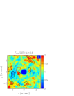
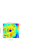
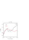
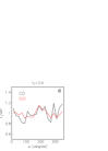
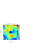
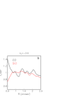
Figure 18: Comparing CO(2-1) and SiO(5-4) emissions (combined data) in the polar outflows: two examples (in the red-shifted hemisphere, upper row and in the blue-shifted hemisphere, lower row). Left pair of panels: normalized channel maps for $V_{z}$=3.6 km s^-1 and $V_{z}$=$-$3.5 km s^-1. We have circled in black some features common to both the CO and SiO maps and in red others that are seen in only one of the two maps. Central panels: normalized $R$ and $\omega$ distributions for CO(2-1) (black) and SiO(5-4) (red), respectively. Right: correlation between the normalised brightness of the two lines; the line is the best fit result (see text).

This analysis gives therefore evidence for two major contributions to the high velocity wings of the SiO(5-4) Doppler velocity spectrum: one, extending up to some 12 km s^-1, is simply the upper edge of the velocity distribution of the polar outflows; the other, reaching up to 20 km s^-1, is confined to the close neighbourhood of the star and corresponds to what is observed in all other oxygen-rich AGB stars where this region of the CSE has been carefully explored. The interpretation given by Tuan-Anh et al. (2019) of these high velocity wings, using data of lower angular resolution, was mixing both contributions. This is clearly illustrated in Figure 20, which displays PV maps of $|V_{z}|$ vs $R$ for both line emissions and both hemispheres separately. In all four cases there is evidence for a clear separation between the two contributions, even if significant differences exist between the CO(2-1) and SiO(5-4) lines as well as between the red-shifted and blue-shifted hemispheres. Another illustration is given by the intensity maps displayed in the left pair of panels of Figure 21 for 8$<$$|V_{z}|$$<$12 km s^-1 (combined data) and in the right pair of panels of the same figure for 12$<$$|V_{z}|$$<$20 km s^-1 (TM0 data). The former give evidence for the above-mentioned asymmetry between blue-shifted and red-shifted hemispheres along the projection of the CSE axis, while the latter display instead a small elongation in the perpendicular direction, possibly revealing the effect of rotation previously observed in SO₂ and CO line emissions. This latter high $V_{z}$ component seems however different from what we know of other stars by the absence of red-shifted absorption, usually interpreted as evidence for in-falling gas, over the stellar disc (Figure 22). Unfortunately, the lack of reliable light curve measurements prevents commenting on a possible relation with the stellar phase at the time of observations. When compared with other nearby oxygen-rich AGB stars, both the velocity of high $V_{z}$ wings and the radial extension of the line broadening region are on the high side; the latter is particularly true when compared with the stellar radius, which, in contrast, is very much on the low side.

6 Summary and discussion

Collecting the information obtained in both the present work and earlier publications to draw a credible picture of the morpho-kinematics of the CSE of EP Aquarii is challenging. The credibility of the interpretation given by Homan et al. (2020), giving a major role to a white dwarf companion currently located at $\sim$400 mas west of the star, has been seriously reduced by the results of the analyses made in the present work: the evidence for a spiral enhancement of CO(2-1) emission has been shown to be weak (Section 3.3); the interpretation of the lumps of CO(2-1) emission in the neighbourhood of the star illustrated in Figure A12 of Homan et al. (2020) can clearly not be claimed as serious evidence for the birth of two spirals; the detailed study of the depression of SiO(5-4) emission presented in Section 4.3 cannot give strong support to an interpretation in terms of dissociation by UV radiation from a white dwarf companion. This does not mean that one can exclude the presence of a companion and its possible role in shaping the CSE. In particular, there is no reason to doubt that EP Aquarii, as most other stars, has several planets orbiting it, some of which may already have been engulfed. But the complexity of the observed morpho-kinematics, and the resulting difficulty to give a reliable interpretation of its many features, prevent claiming a credible model of the mechanisms at stake with sufficient confidence.

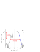
Figure 19: (a): definition of the quantity FWTM (see text) taking as example the Doppler velocity spectrum of SiO(5-4) line emission measured in the ring 60$<$$R$$<$80 mas (see Figure S4 of the supplementary material). The blue line is used to extrapolate the spectrum (using a linear ordinate scale), its intersection with continuum level defining $V_{\text{max}}$ (see text). (b): dependence of FWTM on the ring radius, $R$. The line is a fit 21.3+19.0 exp($-$$R$/0.10) km s^-1. (c,d): measured values of $F(R)$ (c) and of $V_{0}(\omega)$ (d) are compared with the best fit of a form $V_{\text{max}}$=$F(R)V_{0}(\omega)$; the rms deviation to the data is 0.36 km s^-1.

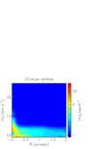
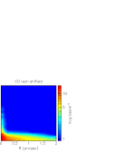
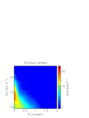
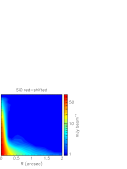
Figure 20: High Doppler velocities (combined data): PV maps of $|V_{z}|$ vs $R$ for both hemispheres and both lines separately, as indicated on top of each panel.

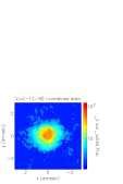
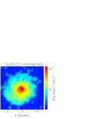
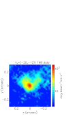
Figure 21: Left: intensity maps of the SiO(5-4) emission (combined data) measured in the Doppler velocity intervals 8$<$$|V_{z}|$$<$12 km s^-1. Right: intensity maps of the SiO(5-4) emission (TM0 data) measured in the Doppler velocity intervals 12$<$$|V_{z}|$$<$20 km s^-1.

In general, the global morpho-kinematics of CO(2-1) emission observed in the present work confirms the results of earlier analyses. The evidence for approximate axi-symmetry about an axis making an angle of $\sim$10^∘ with the line of sight and projecting $\sim$20^∘ west of north on the plane of the sky has been strengthened by observations of both the EDE and polar outflows. The latitudinal dependence of the expansion velocity, evolving from $\sim$2 km s^-1 to $\sim$10 km s^-1 from equator to poles, has been shown to imply a sin${}^{n}\alpha$ term with $n$ smaller than unity, in contrast with the assumption of $n$=2 made by Hoai et al. (2019) (Section 4.1). Evidence for enhancements of emission, in the form of eccentric arcs covering a few tens of degrees, and with a peak to valley ratio well below a factor 2, has been found in both CO(2-1) and SiO(5-4) emission, as well as both in the EDE and polar outflows (Sections 3.3, 4.1 and 4.4). The morphology of these enhancements, which are often, but not always, observed in coincidence between the SiO and CO emissions, suggests that they may be caused by shock waves associated with the lumpy emission of gas from the star atmosphere.

Figure 22: Doppler velocity spectra of SiO(5-4) (upper panels) and CO(2-1) (lower panels) line emissions (TM0 data) integrated in rings as indicated on top of the upper panels.

The birth of the equatorial enhancement observed in CO(2-1) emission has been shown to occur very close to the star, first dominated by rotation, then by expansion, becoming particularly clear at distances exceeding $\sim$200 mas below which important effective line broadening and dust formation are known to be present (Section 3.1). Lack of evidence for a similar enhancement in SiO(5-4) emission is puzzling; only a very small enhancement is visible at distances exceeding $\sim$300 mas (Section 3.2). This suggests that a disc is formed at short distances from the star probably as a result of sufficiently rapid rotation, possibly caused by the recent engulfment of a companion; but this is pure speculation. Understanding the radial evolution of the relative SiO and CO abundances in the disc would require accounting for absorption, which cannot be done reliably with the present data. An intrinsic rms width of nearly 1 km s^-1 has been found to contribute to the EDE flaring of $\sim$40^∘ FWHM evaluated earlier (Hoai et al., 2019). An important remark is that having a proper interpretation for the formation of the EDE automatically provides an interpretation for the polar outflows: the interaction between the EDE and a wind produced according to the commonly accepted mechanism (Höfner & Freytag, 2019) naturally implies that the radial expansion velocity must decrease from the polar value of $\sim$10 km s^-1 to the equatorial value of $\sim$2 km s^-1.

The strong difference between the morpho-kinematics displayed by the SiO(5-4) and CO(2-1) emissions (Section 4.2) was understood as being largely due to the different radial ranges being explored, the former declining rapidly as a result of accretion by dust grains and dissociation by the interstellar UV radiation. However, evidence for a $\sim$33% difference of SiO(5-4) intensity between red-shifted and blue-shifted hemispheres and, more importantly, for a strong western depression at Doppler velocities between $-$2 and $-$6 km s^-1, cannot be simply explained in this way. Ignoring these features, SiO(5-4) emission can qualitatively be described by the standard mass-loss mechanism at play in other oxygen-rich AGB stars (Höfner & Freytag, 2019), with a typical terminal radial expansion velocity at the scale of 10 km s^-1 and some prolateness caused by the presence of the EDE. But these features are obviously playing an important role in the dynamics at stake, and require proper interpretation.

An attempt in this direction was presented in Section 4.3. Very close to the star, between 0.1 and 0.2 arcsec, SiO(5-4) line emission was shown to be dominated by two outflows, one red-shifted covering the southern hemisphere and the other, blue-shifted, covering the northern hemisphere. The former is emitted at small angle to the line of sight but the latter, closer to the plane of the sky, must interact with the nascent rotating and slowly expanding EDE. When moving away from the star, both outflows become narrower, covering smaller intervals of position angle, and voids appear on their sides, one, strongly red-shifted, at $\sim$200 mas in the north, the other, weakly blue-shifted, at $\sim$400 mas in the west. In order to propose a credible interpretation of the underlying mechanism, we need to understand the details of what precisely causes the progressive disappearance of SiO molecules, of what governs the morpho-kinematics of the EDE, of what kind of dust takes part in the acceleration process, of what are the relative roles of stellar pulsation and convective cell granulation in giving the initial boost to the wind, of which kind of pattern of shock waves is present. Only then could one hope to design a model that would properly describe the observations reported in the present work, in particular to explain the similarities and differences observed between CO(2-1) and SiO(5-4) emissions, to explain what causes the strong western depression (absence of emission or strong absorption by a dense lump of matter?), to unveil the nature of the interaction between the polar outflows and the EDE in the close neighbourhood of the star. Lacking such understanding, we can only speculate about possible scenarios, without being able to claim their validity.

The presence of high velocity wings, extending up to $\sim$20 km s^-1, previously noted in earlier work, has been confirmed and shown to include two distinct components (Section 5): front ends of the polar winds, reaching typically 12 km s^-1 but with weak tails reaching well above; and effective line broadening confined to distances shorter than 200 mas from the centre of the star. The earlier interpretation given by Tuan-Anh et al. (2019), was failing to make the distinction between these two components. The observed line broadening, consistent with similar observations in all other low mass-loss rate oxygen-rich AGB stars observed with sufficient angular resolution and sensitivity, is believed to be due to lumpy emission of shock waves associated with convective cell granulation and stellar pulsation, but a detailed picture is lacking. In particular, the absence of red-shifted SiO(5-4) absorption over the stellar disc, contrasting with observations in other stars for which it is interpreted as evidence for in-falling gas, is surprising. In this context, the lack of recent observations of the light curve, preventing the study of a possible relation with the phase of stellar pulsation, is unfortunate. In general, presently available observations do not allow for telling apart, in the close neighbourhood of the star, the contributions of pulsations, convective cell granulation, EDE formation, and dust condensation.

EP Aquarii is clearly a star from which one should learn more than currently feasible; it deserves being studied in as many details as possible with state-of-the-art instruments; it still leaves us with many open questions, the answers to which would be of great help to improve our understanding of the mechanisms at stake in the generation and development of the wind of oxygen-rich AGB stars. The currently favoured picture, combining the continuous formation of an equatorial disc with more lumpy and episodic mass loss produced according to standard mechanisms, is too complex for its validity to be claimed with confidence. Additional ALMA observations of high angular resolution and sensitivity are needed to tell apart the roles of rotation and expansion within some 100 mas from the centre of the star. New infrared observations of the dust, together with simultaneous monitoring of the light curve, are required to possibly reveal correlation with the stellar phase.

Data Availability

The raw data are available on the ALMA archive: ADS/JAO.ALMA#2016.1.01202.S and ADS/JAO.ALMA#2017.1.00862.S. The calibrated and imaged data underlying this article will be shared on reasonable request to the corresponding author.

Appendix A

References

- Bujarrabal et al. (2021) Bujarrabal V., Agúndez M., Gómez-Garrido M., Kim H., Santander-García M., Alcolea J., Castro-Carrizo A., Mikołajewska J., 2021, A&A, 651, A4
- Castellanos-Ramírez et al. (2021) Castellanos-Ramírez A., Rodríguez-González A., Meliani Z., Rivera-Ortiz P. R., Raga A. C., Cantó J., 2021, MNRAS, 507, 4044
- Doan et al. (2017) Doan L., et al., 2017, A&A, 605, A28
- Doan et al. (2020) Doan L., et al., 2020, A&A, 633, A13
- Dumm & Schild (1998) Dumm T., Schild H., 1998, New Astron., 3, 137
- Eggen (1973) Eggen O. J., 1973, Mem. RAS, 77, 159
- Gaia Collaboration (2018) Gaia Collaboration 2018, VizieR Online Data Catalog, p. I/345
- García-Segura et al. (2005) García-Segura G., López J. A., Franco J., 2005, ApJ, 618, 919
- Heras & Hony (2005) Heras A. M., Hony S., 2005, A&A, 439, 171
- Hoai et al. (2019) Hoai D. T., et al., 2019, MNRAS, 484, 1865
- Hoai et al. (2020) Hoai D. T., Tuan-Anh P., Nhung P. T., Darriulat P., Diep P. N., Phuong N. T., Thai T. T., 2020, MNRAS, 495, 943
- Höfner & Freytag (2019) Höfner S., Freytag B., 2019, A&A, 623, A158
- Homan et al. (2018) Homan W., Richards A., Decin L., de Koter A., Kervella P., 2018, A&A, 616, A34
- Homan et al. (2020) Homan W., Cannon E., Montargès M., Richards A. M. S., Millar T. J., Decin L., 2020, A&A, 642, A93
- Lebzelter & Hron (1999) Lebzelter T., Hron J., 1999, A&A, 351, 533
- Liimets et al. (2018) Liimets T., et al., 2018, A&A, 612, A118
- Melnikov et al. (2018) Melnikov S., Stute M., Eislöffel J., 2018, A&A, 612, A77
- Nhung et al. (2022) Nhung P. T., Hoai D. T., Tuan-Anh P., Darriulat P., Diep P. N., Ngoc N. B., Thai T. T., 2022, ApJ, 927, 169
- Nordhaus & Blackman (2006) Nordhaus J., Blackman E. G., 2006, MNRAS, 370, 2004
- Olofsson et al. (2019) Olofsson H., et al., 2019, A&A, 623, A153
- Sahai et al. (2022) Sahai R., Huang P. S., Scibelli S., Morris M. R., Hinkle K., Lee C. F., 2022, ApJ, 929, 59
- Tabur et al. (2009) Tabur V., Bedding T. R., Kiss L. L., Moon T. T., Szeidl B., Kjeldsen H., 2009, MNRAS, 400, 1945
- Tuan-Anh et al. (2019) Tuan-Anh P., et al., 2019, MNRAS, 487, 622
- Winters et al. (2022) Winters J. M., et al., 2022, A&A, 658, A135
- van Leeuwen (2007) van Leeuwen F., 2007, Hipparcos, the New Reduction of the Raw Data. Astrophysics and Space Science Library Vol. 350, Springer Science+Business Media B.V., doi:10.1007/978-1-4020-6342-8