Effects of Non-minimal Matter-geometry Coupling on Embedding Class-one Anisotropic Solutions

Abstract

This paper investigates some particular anisotropic star models in $f(\mathcal{R},\mathcal{T},\mathcal{Q})$ gravity, where $\mathcal{Q}=\mathcal{R}_{\omega\alpha}\mathcal{T}^{\omega\alpha}$. We adopt a standard model $f(\mathcal{R},\mathcal{T},\mathcal{Q})=\mathcal{R}+\varpi\mathcal{Q}$, where $\varpi$ indicates a coupling constant. We take spherically symmetric spacetime and develop solutions to the modified field equations corresponding to different choices of the matter Lagrangian by applying ‘embedding class-one’ scheme. For this purpose, we utilize $\mathbb{MIT}$ bag model equation of state and investigate some physical aspects of compact models such as RXJ 1856-37, 4U 1820-30, Cen X-3, SAX J 1808.4-3658 and Her X-I. We use masses and radii of these stars and employ the vanishing radial pressure condition at the boundary to calculate the value of their respective bag constant $\mathfrak{B_{c}}$. Further, we fix $\varpi=\pm 4$ to analyze the behavior of resulting state variables, anisotropy, mass, compactness, surface redshift as well as energy bounds through graphical interpretation for each star model. Two different physical tests are performed to check the stability of the developed solutions. We conclude that $\varpi=-4$ is more suitable choice for the considered modified model to obtain stable structures of the compact bodies.

Keywords: $f(\mathcal{R},\mathcal{T},\mathcal{R}_{\omega\alpha}\mathcal{T}^{\omega\alpha})$ gravity; Anisotropy; Compact stars.
PACS: 04.50.Kd; 04.40.Dg; 04.40.-b.

1 Introduction

Although General Relativity ($\mathbb{GR}$) has made tremendous achievements in elucidating many unknown components of our universe, it is insufficient to investigate cosmic structure at vast scale. In the recent era, several modifications to $\mathbb{GR}$ have been postulated to disclose the perplexing issues which are associated with the cosmic evolution such as its rapid expansion and dark matter etc. This expansion results in the existence of an obscure form of force, named as dark energy having immensely large negative pressure. Therefore, the modified theories are viewed as remarkably significant in exposing the cosmic mysterious features. Firstly, the geometric part of Einstein-Hilbert action was modified to obtain $f(\mathcal{R})$ theory which is straightforward generalization to $\mathbb{GR}$ due to the insertion of generic function of the Ricci scalar in place of $\mathcal{R}$. Various authors [1]-[5] have studied the celestial structures in this theory and analyzed their feasibility through different schemes. Multiple forms of $f(\mathcal{R})$ gravity have been considered to study several cosmological problems, i.e., late-time evolution of the universe [6, 7], the inflationary era [8] and background of cosmic expansion [9, 10].

Bertolami et al. [11] analyzed the influence of matter-geometry coupling on stellar systems in $f(\mathcal{R})$ scenario for the very first time by adopting the matter Lagrangian in form of $\mathcal{R}$ and $\mathbb{L}_{m}$. Many researchers have been prompted by such interaction, as a result of which they payed their concentration in investigating cosmic rapid expansion. A couple of years ago, several modified gravitational theories were proposed comprising an arbitrary coupling in some general manner at the action level which ultimately turns out to be a subject of great importance for astrophysicists. The $f(\mathcal{R},\mathcal{T})$ gravity which encompasses such interaction is contemplated by Harko et al. [12], in which $\mathcal{T}$ demonstrates trace of the energy-momentum tensor $(\mathbb{EMT})$. The modified functional forms involving $\mathcal{T}$ give rise to the non-conserved $\mathbb{EMT}$ unlike $\mathbb{GR}$ and $f(\mathcal{R})$ theories. Numerous scientists [13]-[18] investigated different massive structures in $f(\mathcal{R},\mathcal{T})$ framework and found that this gravity yields several fascinating astrophysical outcomes. To get better understanding of cosmic inflationary era, an even more complex functional $f(\mathcal{R},\mathcal{T},\mathcal{Q})$ is suggested by Haghani et al. [19], where $\mathcal{Q}$ indicates the contraction of the Ricci tensor and $\mathbb{EMT}$ (i.e., $\mathcal{Q}\equiv\mathcal{R}_{\omega\alpha}\mathcal{T}^{\omega\alpha}$). They deemed certain mathematical models to study their physical feasibility and employed Lagrange multiplier method to obtain conservation of the $\mathbb{EMT}$.

The development of this modified gravity was premised on the insertion of the factor $\mathcal{Q}$ which ensures the presence of strong non-minimal matter-geometry coupling in self-gravitating systems. The modification in the Einstein-Hilbert action may help in explaining the role of dark energy and dark matter, without resorting to exotic fluid distribution. Some other extensions to $\mathbb{GR}$ like $f(\mathcal{R},\mathbb{L}_{m})$ and $f(\mathcal{R},\mathcal{T})$ gravitational theories also comprise the matter Lagrangian involving such arbitrary interaction but we cannot consider their functionals as the most generalized form that provide proper understanding to the influence of coupling on self-gravitating objects in some scenarios. It must be noted here that the factor $\mathcal{R}_{\omega\alpha}\mathcal{T}^{\omega\alpha}$ could explain the impact of non-minimal interaction in the situation where $f(\mathcal{R},\mathcal{T})$ theory breaks down to achieve such results. In particular, $f(\mathcal{R},\mathcal{T})$ fails to uphold the non-minimal coupling for the case when $\mathcal{T}=0$ inside the configuration, however, this phenomenon can be explained by $f(\mathcal{R},\mathcal{T},\mathcal{Q})$ gravity. Due to the non-conservation of energy-momentum tensor in this theory, an additional force is present due to which the motion of test particles in geodesic path comes to an end. This force also helps to elucidate the galactic rotation curves. Sharif and Zubair [20] assumed two models such as $\mathcal{R}+\varpi\mathcal{Q}$ and $\mathcal{R}(1+\varpi\mathcal{Q})$ to study thermodynamical laws for black holes with different choices of matter Lagrangian like $\mathbb{L}_{m}=\rho$ as well as $-p$ and obtained their viability constraints. They also explored energy conditions corresponding to the above models and concluded that weak energy conditions are satisfied only when $\varpi>0$ [21].

Odintsov and Sáez-Gómez [22] studied various cosmological solutions and the occurrence of $\Lambda$CDM model in $f(\mathcal{R},\mathcal{T},\mathcal{Q})$ gravity. They also discussed the issue related to matter instability and figured out that this theory may permit to generate pure de Sitter universe subject to the usability of non-constant fluids. An important requirement usually demanded by extended theories consists of the avoidance of the Ostrogradski as well as Dolgov-Kawasaki instability. The later issue has recently been addressed for this theory [19, 22]. Ayuso et al. [23] showed that conformal as well as strong non-minimal matter-geometry couplings oftenly produce higher-order equations of motion and illustrated this phenomenon by adopting certain appropriate scalar as well as massive vector fields. It is found that ghost modes are generally present in these theories due to the coupling $\mathcal{R}_{\omega\alpha}\mathcal{T}^{\omega\alpha}$ and that its avoidance considerably restricts the allowed form for the functional $f$. Different models in this theory have been studied, one of them is the $f(\mathcal{R},\mathcal{T},\mathcal{Q})=\beta(\mathcal{R})^{n}+\varpi(\mathcal{Q})^{m}$, where $\beta$ and $\varpi$ are real-valued coupling constants. It is shown that this theory will be free of Ostrogradski instabilities for $n=1=m$.

Baffou et al. [24] obtained Friedmann equations and developed the stability of this theory for two different models by calculating numerical solution of the perturbation functions as well as power-law and de Sitter solutions. Sharif and Waseem [25] calculated the solutions corresponding to the isotropic/anisotropic configurations by choosing different matter Lagrangian and discussed their stability through various approaches. Yousaf et al. [26]-[31] studied the structural evolution of spherical and cylindrical celestial bodies with the help of modified structure scalars which came from orthogonal decomposition of the Riemann tensor. We have utilized the decoupling technique to get physically acceptable charged/uncharged solutions to the $f(\mathcal{R},\mathcal{T},\mathcal{Q})$ field equations [32, 33].

Stars are acknowledged as indispensable components of our galaxy among the plenty of unfathomable constituents of the universe. The structural formation of such objects encouraged many astrophysicists that they would pay attention on the study of their developmental phases. Neutron stars gained much attention amongst all compact bodies in virtue of their intriguing properties. The mass of a neutron star is approximately 1 to 3 times solar masses ($M_{\bigodot}$) and its core contains newly formed neutrons which help to produce degeneracy pressure to counterbalance the gravitational force and resist that neutron to further collapse. The first ever neutron star was predicted in 1934 [34], but observationally, it was confirmed later. This is due to the fact that neutron stars do not release sufficient radiations and are mostly indiscernible. Another highly dense object between neutron star and black hole is the quark star whose interior is filled with up, down and strange quark matter. Numerous research has been done on the study of formation of such hypothetical structures [35]-[38].

At present time, the study of compact bodies whose interiors contain anisotropic matter configuration have become a persuasive subject of research for numerous astronomers. According to Herrera’ observation [39], a celestial object comprising nuclear density in its core much lower than the mass density should be owned by anisotropic fluid. Herrera and Santos [40] discussed the self-gravitating structures and analyzed impressive effects of anisotropy on those bodies. Harko and Mak [41] inspected the feasibility of anisotropic solutions corresponding to static relativistic objects. Hossein et al. [42] considered Krori-Barua solution to analyze stability of the anisotropic massive systems by including the impact of cosmological constant $\Lambda$. Kalam et al. [43] constructed solutions of gravitational equations of motion corresponding to various neutron stars and found them viable as well as stable. Paul and Deb [44] developed certain feasible solutions for compact stars which were considered in hydrostatic equilibrium.

The matter distribution inside quark bodies contains physical variables such as energy density and pressure, thus in this regard, the $\mathbb{MIT}$ bag model equation of state ($\mathbb{E}$o$\mathbb{S}$) is viewed as an effective tool which interrelates these quantities [45]. It has also been observed that this model can efficiently describe the compactness of various structures such as PSR 0943+10, 4U 1820-30, 4U 1728-34, RXJ 185635-3754, Her X-1 and SAX J 1808.4-3658, etc., while the neutron star $\mathbb{E}$o$\mathbb{S}$ flunks in this context [46]. Generally, a vacuum involves true and false states whose discrepency can be determined by the bag constant ($\mathfrak{B_{c}}$) and its increasing value results in lowering quark pressure. Several researchers [47]-[49] analyzed different quark stars and their internal formation with the help of $\mathbb{MIT}$ bag model. Demorest et al. [50] quantified the mass of a quark star (namely, PSR J1614-2230) and concluded that only this model can support such kind of heavily objects. The mass of various compact structures has been measured by Rahaman et al. [51] by employing an interpolating technique and they also studied some physical aspects of a star candidate having radius as 9.9km.

Several techniques have been used in literature to formulate solution to the field equations such as the solution of metric potentials or by making use of a particular $\mathbb{E}$o$\mathbb{S}$. An embedding class-one technique is one of them which states that $(n-2)$-dimensional space can be embedded into an $(n-1)$-dimensional space. Bhar et al. [52] utilized this scheme along with a new metric coefficient to find physically feasible solutions for anisotropic systems. Maurya et al. [53, 54] calculated the embedding class-one solution and analyzed its stability as well as effects of anisotropy on relativistic stars. By suggesting a particular metric function, Singh et al. [55] formed singularity-free solution for spherical geometry with the help of this technique. This work has been extended by Sharif and his collaborators [56]-[62]. They found stable as well as viable solutions in different theories like $f(\mathcal{R},\mathcal{T})$, Brans-Dicke and $f(\mathcal{G})$ gravity.

In this paper, we analyze physical feasibility of two solutions to the modified field equations corresponding to different forms of matter Lagrangian in $f(\mathcal{R},\mathcal{T},\mathcal{R}_{\omega\alpha}\mathcal{T}^{\omega\alpha})$ theory. The following lines help to understand that how the paper is structured. In the next section, we construct the field equations in modified gravity for a particular model ($\mathcal{R}+\varpi\mathcal{R}_{\omega\alpha}\mathcal{T}^{\omega\alpha}$), where we fix $\varpi=\pm 4$. Further, we assume $\mathbb{MIT}$ bag model $\mathbb{E}$o$\mathbb{S}$ to solve the field equations, take one metric potential and employ embedding class-one condition to find the other. Section 3 calculates the four unknowns $(W,X,Y,Z)$ at the hypersurface. Various physical characteristics of compact stars are analyzed through graphical interpretation in section 4. Lastly, the concluded remarks are presented in section 5.

2 The $f(\mathcal{R},\mathcal{T},\mathcal{R}_{\omega\alpha}\mathcal{T}^{\omega\alpha})$ Gravity

The modified form of Einstein-Hilbert action in terms of complex analytical functional $f(\mathcal{R},\mathcal{T},\mathcal{R}_{\omega\alpha}\mathcal{T}^{\omega\alpha})$ (with $\kappa=8\pi$) is given as [22]

$$S_{f(\mathcal{R},\mathcal{T},\mathcal{R}_{\omega\alpha}\mathcal{T}^{\omega\alpha})}=\int\sqrt{-g}\left[\frac{f(\mathcal{R},\mathcal{T},\mathcal{R}_{\omega\alpha}\mathcal{T}^{\omega\alpha})}{16\pi}+\mathbb{L}_{m}\right]d^{4}x,$$ (1)

where $\mathbb{L}_{m}$ serves as the matter Lagrangian. After applying the variational principle on the action (1), we obtain the field equations as

$$\mathcal{G}_{\omega\alpha}=\mathcal{T}_{\omega\alpha}^{(eff)}=8\pi\bigg{(}\frac{\mathcal{T}_{\omega\alpha}}{f_{\mathcal{R}}-\mathbb{L}_{m}f_{\mathcal{Q}}}+\mathcal{T}_{\omega\alpha}^{(\mathcal{C})}\bigg{)},$$ (2)

which describe matter in terms of spacetime. Here, $\mathcal{G}_{\omega\alpha}$ represents the geometrical structure and $\mathcal{T}_{\omega\alpha}^{(eff)}$ is the $\mathbb{EMT}$ in modified gravity which involves state variables along with their derivatives. Thus the sector $\mathcal{T}_{\omega\alpha}^{(\mathcal{C})}$ appearing due to the insertion of additional term $\mathcal{R}_{\omega\alpha}\mathcal{T}^{\omega\alpha}$ in the action (1) is given as

$$\mathcal{T}_{\omega\alpha}^{(\mathcal{C})} = \frac{1}{8\pi\left(f_{\mathcal{R}}-\mathbb{L}_{m}f_{\mathcal{Q}}\right)}\left[\bigg{(}f_{\mathcal{T}}+\frac{1}{2}\mathcal{R}f_{\mathcal{Q}}\bigg{)}\mathcal{T}_{\omega\alpha}+\left\{\frac{\mathcal{R}}{2}(\frac{f}{\mathcal{R}}-f_{\mathcal{R}})-\mathbb{L}_{m}f_{\mathcal{T}}\right.\right.$$ (3)

$$- \left.\frac{1}{2}\nabla_{\sigma}\nabla_{\xi}(f_{\mathcal{Q}}\mathcal{T}^{\sigma\xi})\right\}g_{\omega\alpha}-\frac{1}{2}\Box(f_{\mathcal{Q}}\mathcal{T}_{\omega\alpha})-(g_{\omega\alpha}\Box-\nabla_{\omega}\nabla_{\alpha})f_{\mathcal{R}}$$

$$- 2f_{\mathcal{Q}}\mathcal{R}_{\sigma(\omega}\mathcal{T}_{\alpha)}^{\sigma}+\nabla_{\sigma}\nabla_{(\omega}[\mathcal{T}_{\alpha)}^{\sigma}f_{\mathcal{Q}}]+2(f_{\mathcal{Q}}\mathcal{R}^{\sigma\xi}+\left.f_{\mathcal{T}}g^{\sigma\xi})\frac{\partial^{2}\mathbb{L}_{m}}{\partial g^{\omega\alpha}\partial g^{\sigma\xi}}\right],$$

where $f_{\mathcal{R}}=\frac{\partial f(\mathcal{R},\mathcal{T},\mathcal{Q})}{\partial\mathcal{R}},~{}f_{\mathcal{T}}=\frac{\partial f(\mathcal{R},\mathcal{T},\mathcal{Q})}{\partial\mathcal{T}}$ and $f_{\mathcal{Q}}=\frac{\partial f(\mathcal{R},\mathcal{T},\mathcal{Q})}{\partial\mathcal{Q}}$. Also, $\nabla_{\omega}$ and $\Box\equiv\frac{1}{\sqrt{-g}}\partial_{\omega}\big{(}\sqrt{-g}g^{\omega\alpha}\partial_{\alpha}\big{)}$ represent covariant derivative and the D’Alambert operator, respectively. The attractive nature of this modified gravity needs to satisfy the following constraint

$$\frac{8\pi+f_{\mathcal{T}}+\frac{1}{2}\mathcal{R}f_{\mathcal{Q}}}{f_{\mathcal{R}}-\mathbb{L}_{m}f_{\mathcal{Q}}}>0.$$

The modified field equations involve explicit form of the matter Lagrangian, thus the corresponding dynamics can be studied by taking some particular form of this Lagrangian. Different choices of the matter Lagrangian for a perfect fluid have been analyzed in literature. These include $\mathbb{L}_{m}=\pm{P}$ [63], $\mathbb{L}_{m}=\pm{\mu}$ [64] and $\mathbb{L}_{m}=\mathcal{T}$ [65], where $P$ and $\mu$ are isotropic pressure and energy density, respectively. The sign depends on the signature of the chosen metric. As we have considered anisotropic matter distribution in the interior of quark stars, thus the Lagrangian $\mathbb{L}_{m}$ in terms of pressure $P$ can now be taken as $P_{r}$ (radial pressure) and $P_{\bot}$ (tangential pressure). Finally, we have three choices of the matter Lagrangian in this case as $\mu,~{}P_{r}$ and $P_{\bot}$. According to the signatures ($-,+,+,+$), one can take $\mathbb{L}_{m}=-\mu,~{}P_{r}$ and $P_{\bot}$. Here, we adopt first two forms (which has been extensively employed) to obtain the solutions of modified field equations and to analyze the effects of strong matter-geometry coupling on them. These choices lead to $\frac{\partial^{2}\mathbb{L}_{m}}{\partial g^{\omega\alpha}\partial g^{\sigma\xi}}=0$ [19]. The choice $\mathbb{L}_{m}=P_{\bot}$ can also be taken which may produce acceptable results in this theory.

The covariant divergence of the effective $\mathbb{EMT}$ has the form

$$\nabla^{\omega}\mathcal{T}_{\omega\alpha}^{(eff)}=0,$$

which consequently leads to

$$\nabla^{\omega}\mathcal{T}_{\omega\alpha} =\frac{2}{2f_{\mathcal{T}}+\mathcal{R}f_{\mathcal{Q}}+16\pi}\bigg{[}\nabla_{\omega}\big{(}f_{\mathcal{Q}}\mathcal{R}^{\sigma\omega}\mathcal{T}_{\sigma\alpha}\big{)}-\mathcal{G}_{\omega\alpha}\nabla^{\omega}\big{(}f_{\mathcal{Q}}\mathbb{L}_{m}\big{)}-\frac{1}{2}\nabla_{\alpha}\mathcal{T}^{\sigma\xi}$$

$$\times\big{(}f_{\mathcal{T}}g_{\sigma\xi}+f_{\mathcal{Q}}\mathcal{R}_{\sigma\xi}\big{)}+\nabla_{\alpha}\big{(}\mathbb{L}_{m}f_{\mathcal{T}}\big{)}-\frac{1}{2}\big{\{}\nabla^{\omega}(\mathcal{R}f_{\mathcal{Q}})+2\nabla^{\omega}f_{\mathcal{T}}\big{\}}\mathcal{T}_{\omega\alpha}\bigg{]}.$$ (4)

The $\mathbb{EMT}$ is mainly used to describe the distribution of matter in the interior of astronomical systems and its each non-null component is related to a particular physical property of the structure. The anisotropy (occurs when the pressure in radial and tangential directions are different) in celestial objects is considered as a valuable factor in examining the evolution of their structures. Our cosmos contains a number of massive objects and most of them are considered to be interlinked with anisotropic distribution, therefore this factor has important implications for stellar models in their evolutionary phases. Hence, we assume the following $\mathbb{EMT}$ representing anisotropic configuration as

$$\mathcal{T}_{\omega\alpha}=(\mu+P_{\bot})\mathcal{K}_{\omega}\mathcal{K}_{\alpha}+P_{\bot}g_{\omega\alpha}+\left(P_{r}-P_{\bot}\right)\mathcal{W}_{\omega}\mathcal{W}_{\alpha},$$ (5)

where the quantities $\mathcal{W}_{\omega}$ and $\mathcal{K}_{\omega}$ indicate the four-vector and the four-velocity, respectively. The trace of $f(\mathcal{R},\mathcal{T},\mathcal{Q})$ field equations become as

$$3\nabla^{\sigma}\nabla_{\sigma}f_{\mathcal{R}}-\mathcal{R}\left(\frac{\mathcal{T}}{2}f_{\mathcal{Q}}-f_{\mathcal{R}}\right)-\mathcal{T}(8\pi+f_{\mathcal{T}})+\frac{1}{2}\nabla^{\sigma}\nabla_{\sigma}(f_{\mathcal{Q}}\mathcal{T})$$

$$-2f+\nabla_{\omega}\nabla_{\sigma}(f_{\mathcal{Q}}\mathcal{T}^{\omega\sigma})+(\mathcal{R}f_{\mathcal{Q}}+4f_{\mathcal{T}})\mathbb{L}_{m}+2\mathcal{R}_{\omega\sigma}\mathcal{T}^{\omega\sigma}f_{\mathcal{Q}}$$

$$-2g^{\alpha\xi}\frac{\partial^{2}\mathbb{L}_{m}}{\partial g^{\alpha\xi}\partial g^{\omega\sigma}}\left(f_{\mathcal{T}}g^{\omega\sigma}+f_{\mathcal{Q}}R^{\omega\sigma}\right)=0.$$

The insertion of $\mathcal{Q}=0$ in the overhead equation vanishes the effects of strong non-minimal coupling in the interior of stellar object and produces $f(\mathcal{R},\mathcal{T})$ theory, which further reduces to the $f(\mathcal{R})$ gravity after implementing the vacuum scenario.

We assume spherical spacetime to discuss the internal matter distribution of compact stars as

$$ds^{2}=-e^{\rho}dt^{2}+e^{\zeta}dr^{2}+r^{2}d\theta^{2}+r^{2}\sin^{2}\theta d\psi^{2},$$ (6)

where $\rho=\rho(r)$ and $\zeta=\zeta(r)$. This produces four-vector and four-velocity in comoving coordinates as

$$\mathcal{W}^{\omega}=\delta^{\omega}_{1}e^{\frac{-\zeta}{2}},\quad\mathcal{K}^{\omega}=\delta^{\omega}_{0}e^{\frac{-\rho}{2}},$$ (7)

which must satisfy $\mathcal{K}^{\omega}\mathcal{K}_{\omega}=-1$ and $\mathcal{W}^{\omega}\mathcal{K}_{\omega}=0$, as we consider the signatures of geometry (6) $(-,+,+,+)$. Our universe is currently passing through accelerating expansion phase and consists of numerous stars existing in non-linear regime, but the study of their linear behavior may provide better understanding about the structural formation of these massive bodies. In contrast to $f(\mathcal{R},\mathbb{L}_{m})$ and $f(\mathcal{R},\mathcal{T})$ theories, the factor $\mathcal{R}_{\omega\alpha}\mathcal{T}^{\omega\alpha}$ is responsible to make $f(\mathcal{R},\mathcal{T},\mathcal{Q})$ gravity much complicated. Haghani et al. [19] discussed cosmological applications of three different models in this framework, i.e., $\mathcal{R}+\varpi\mathcal{Q},~{}\mathcal{R}(1+\varpi\mathcal{Q})$ and $\mathcal{R}+\beta\sqrt{\mid\mathcal{T}\mid}+\varpi\mathcal{Q}$, where $\varpi$ and $\beta$ are arbitrary coupling constants. They analyzed the evolution and dynamics of the universe for the above models with and without energy conservation. We thus consider the following model to analyze five different star candidates as

$$f(\mathcal{R},\mathcal{T},\mathcal{R}_{\omega\alpha}\mathcal{T}^{\omega\alpha})=f_{1}(\mathcal{R})+f_{2}(\mathcal{R}_{\omega\alpha}\mathcal{T}^{\omega\alpha})=\mathcal{R}+\varpi\mathcal{R}_{\omega\alpha}\mathcal{T}^{\omega\alpha}.$$ (8)

In this case, if $\varpi>0$, the solution has an oscillatory behavior with alternating expanding and collapsing phases. For $\varpi<0$, the scale factor of the universe has a hyperbolic cosine-type dependence. Since $\varpi$ is any real-valued coupling constant, thus one can take any value (positive or negative) to check whether the corresponding solution is physically acceptable or not. In this regard, we choose it as $\varpi=\pm 4$.

It is interesting to stress that physical feasibility of different gravity models can be achieved by taking the value of coupling parameter within its observed range. The model (8) has been utilized in several investigations based on the stability and viability of various isotropic and anisotropic configured stars [20, 21, 25]. In this case, $\mathcal{Q}$ becomes

$$\mathcal{Q} = e^{-\zeta}\bigg{[}\frac{\mu}{4}\left(\rho^{\prime 2}-\rho^{\prime}\zeta^{\prime}+2\rho^{\prime\prime}+\frac{4\rho^{\prime}}{r}\right)-\frac{P_{r}}{4}\left(\rho^{\prime 2}-\rho^{\prime}\zeta^{\prime}+2\rho^{\prime\prime}+\frac{4\zeta^{\prime}}{r}\right)$$

$$+ P_{\bot}\left(\frac{\zeta^{\prime}}{r}-\frac{\rho^{\prime}}{r}+\frac{2e^{\zeta}}{r^{2}}-\frac{2}{r^{2}}\right)\bigg{]}.$$

Here, ${}^{\prime}=\frac{\partial}{\partial r}$. We use Eqs.(2) and (3) together along with the model (8) to construct modified field equations as

$$\mathcal{G}_{\omega\alpha} = \frac{\varpi}{1-\varpi\mathbb{L}_{m}}\bigg{[}\left(\frac{8\pi}{\varpi}+\frac{1}{2}\mathcal{R}\right)\mathcal{T}_{\omega\alpha}+\frac{1}{2}\left\{\mathcal{Q}-\nabla_{\sigma}\nabla_{\xi}\mathcal{T}^{\sigma\xi}\right\}g_{\omega\alpha}-2\mathcal{R}_{\sigma(\omega}\mathcal{T}_{\alpha)}^{\sigma}$$

$$- \frac{1}{2}\Box\mathcal{T}_{\omega\alpha}+\nabla_{\sigma}\nabla_{(\omega}\mathcal{T}_{\alpha)}^{\sigma}+2\mathcal{R}^{\sigma\xi}\frac{\partial^{2}\mathbb{L}_{m}}{\partial g^{\omega\alpha}\partial g^{\sigma\xi}}\bigg{]},$$ (9)

and the covariant divergence (4) becomes

$$\nabla^{\omega}\mathcal{T}_{\omega\alpha} = \frac{2\varpi}{\varpi\mathcal{R}+16\pi}\bigg{[}\nabla_{\omega}(\mathcal{R}^{\sigma\omega}\mathcal{T}_{\sigma\alpha})-\frac{1}{2}\mathcal{R}_{\sigma\xi}\nabla_{\alpha}\mathcal{T}^{\sigma\xi}-\frac{1}{2}\mathcal{T}_{\omega\alpha}\nabla^{\omega}\mathcal{R}-\mathcal{G}_{\omega\alpha}$$ (10)

$$\times \nabla^{\omega}\big{(}\mathbb{L}_{m}\big{)}\bigg{]}.$$

The non-zero components of field equations (9) for the fluid distribution (5) and $\mathbb{L}_{m}=-\mu$ become

$$8\pi\mu =e^{-\zeta}\bigg{[}\frac{\zeta^{\prime}}{r}+\frac{e^{\zeta}}{r^{2}}-\frac{1}{r^{2}}+\varpi\bigg{\{}\mu\bigg{(}\frac{3\rho^{\prime}\zeta^{\prime}}{8}-\frac{\rho^{\prime 2}}{8}+\frac{\zeta^{\prime}}{r}+\frac{e^{\zeta}}{r^{2}}-\frac{1}{r^{2}}-\frac{3\rho^{\prime\prime}}{4}$$

$$-\frac{3\rho^{\prime}}{2r}\bigg{)}-\mu^{\prime}\bigg{(}\frac{\zeta^{\prime}}{4}-\frac{1}{r}-\rho^{\prime}\bigg{)}+\frac{\mu^{\prime\prime}}{2}+P_{r}\bigg{(}\frac{\rho^{\prime}\zeta^{\prime}}{8}-\frac{\rho^{\prime 2}}{8}-\frac{\rho^{\prime\prime}}{4}+\frac{\zeta^{\prime}}{2r}+\frac{\zeta^{\prime\prime}}{2}$$

$$-\frac{3\zeta^{\prime 2}}{4}\bigg{)}+\frac{5\zeta^{\prime}P^{\prime}_{r}}{4}-\frac{P^{\prime\prime}_{r}}{2}+P_{\bot}\bigg{(}\frac{\zeta^{\prime}}{2r}-\frac{\rho^{\prime}}{2r}+\frac{3e^{\zeta}}{r^{2}}-\frac{1}{r^{2}}\bigg{)}-\frac{P^{\prime}_{\bot}}{r}\bigg{\}}\bigg{]},$$ (11)

$$8\pi P_{r} =e^{-\zeta}\bigg{[}\frac{\rho^{\prime}}{r}-\frac{e^{\zeta}}{r^{2}}+\frac{1}{r^{2}}+\varpi\bigg{\{}\mu\bigg{(}\frac{\rho^{\prime}\zeta^{\prime}}{8}+\frac{\rho^{\prime 2}}{8}-\frac{\rho^{\prime\prime}}{4}-\frac{\rho^{\prime}}{2r}\bigg{)}-\frac{\rho^{\prime}\mu^{\prime}}{4}-P_{r}$$

$$\times\bigg{(}\frac{5\rho^{\prime 2}}{8}-\frac{7\rho^{\prime}\zeta^{\prime}}{8}+\frac{5\rho^{\prime\prime}}{4}-\frac{7\zeta^{\prime}}{2r}+\frac{\rho^{\prime}}{r}-\zeta^{\prime 2}-\frac{e^{\zeta}}{r^{2}}+\frac{1}{r^{2}}\bigg{)}+P^{\prime}_{r}\bigg{(}\frac{\rho^{\prime}}{4}+\frac{1}{r}\bigg{)}$$

$$-P_{\bot}\bigg{(}\frac{\zeta^{\prime}}{2r}-\frac{\rho^{\prime}}{2r}+\frac{3e^{\zeta}}{r^{2}}-\frac{1}{r^{2}}\bigg{)}+\frac{P^{\prime}_{\bot}}{r}\bigg{\}}\bigg{]},$$ (12)

$$8\pi P_{\bot} =e^{-\zeta}\bigg{[}\frac{\rho^{\prime 2}}{4}-\frac{\rho^{\prime}\zeta^{\prime}}{4}+\frac{\rho^{\prime\prime}}{2}-\frac{\zeta^{\prime}}{2r}+\frac{\rho^{\prime}}{2r}+\varpi\bigg{\{}\mu\bigg{(}\frac{\rho^{\prime 2}}{8}+\frac{\rho^{\prime}\zeta^{\prime}}{8}-\frac{\rho^{\prime\prime}}{4}-\frac{\rho^{\prime}}{2r}\bigg{)}$$

$$-\frac{\rho^{\prime}\mu^{\prime}}{4}-P_{r}\bigg{(}\frac{\rho^{\prime}\zeta^{\prime}}{8}-\frac{\rho^{\prime 2}}{8}-\frac{\rho^{\prime\prime}}{4}+\frac{\zeta^{\prime}}{2r}+\frac{\zeta^{\prime\prime}}{2}-\frac{3\zeta^{\prime 2}}{4}\bigg{)}-\frac{5\zeta^{\prime}P^{\prime}_{r}}{4}+\frac{P^{\prime\prime}_{r}}{2}$$

$$-P_{\bot}\bigg{(}\frac{\rho^{\prime 2}}{4}-\frac{\rho^{\prime}\zeta^{\prime}}{4}+\frac{\rho^{\prime\prime}}{2}-\frac{\zeta^{\prime}}{r}+\frac{\rho^{\prime}}{r}\bigg{)}-P^{\prime}_{\bot}\bigg{(}\frac{\zeta^{\prime}}{4}-\frac{\rho^{\prime}}{4}-\frac{3}{r}\bigg{)}+\frac{P^{\prime\prime}_{\bot}}{2}\bigg{\}}\bigg{]},$$ (13)

and for $\mathbb{L}_{m}=P_{r}$, we have

$$8\pi\mu =e^{-\zeta}\bigg{[}\frac{\zeta^{\prime}}{r}+\frac{e^{\zeta}}{r^{2}}-\frac{1}{r^{2}}+\varpi\bigg{\{}\mu\bigg{(}\frac{3\rho^{\prime}\zeta^{\prime}}{8}-\frac{\rho^{\prime 2}}{8}+\frac{\zeta^{\prime}}{r}+\frac{e^{\zeta}}{r^{2}}-\frac{3\rho^{\prime\prime}}{4}-\frac{3\rho^{\prime}}{2r}$$

$$-\frac{1}{r^{2}}\bigg{)}-\mu^{\prime}\bigg{(}\frac{\zeta^{\prime}}{4}-\frac{1}{r}-\rho^{\prime}\bigg{)}+\frac{\mu^{\prime\prime}}{2}+P_{r}\bigg{(}\frac{\rho^{\prime}\zeta^{\prime}}{8}-\frac{\rho^{\prime 2}}{8}-\frac{\rho^{\prime\prime}}{4}-\frac{\zeta^{\prime}}{2r}-\frac{e^{\zeta}}{r^{2}}$$

$$+\frac{1}{r^{2}}+\frac{\zeta^{\prime\prime}}{2}-\frac{3\zeta^{\prime 2}}{4}\bigg{)}+\frac{5\zeta^{\prime}P^{\prime}_{r}}{4}-\frac{P^{\prime\prime}_{r}}{2}+P_{\bot}\bigg{(}\frac{\zeta^{\prime}}{2r}-\frac{\rho^{\prime}}{2r}+\frac{3e^{\zeta}}{r^{2}}-\frac{1}{r^{2}}\bigg{)}$$

$$-\frac{P^{\prime}_{\bot}}{r}\bigg{\}}\bigg{]},$$ (14)

$$8\pi P_{r} =e^{-\zeta}\bigg{[}\frac{\rho^{\prime}}{r}-\frac{e^{\zeta}}{r^{2}}+\frac{1}{r^{2}}+\varpi\bigg{\{}\mu\bigg{(}\frac{\rho^{\prime}\zeta^{\prime}}{8}+\frac{\rho^{\prime 2}}{8}-\frac{\rho^{\prime\prime}}{4}-\frac{\rho^{\prime}}{2r}\bigg{)}-\frac{\rho^{\prime}\mu^{\prime}}{4}-P_{r}$$

$$\times\bigg{(}\frac{5\rho^{\prime 2}}{8}-\frac{7\rho^{\prime}\zeta^{\prime}}{8}+\frac{5\rho^{\prime\prime}}{4}-\frac{7\zeta^{\prime}}{2r}+\frac{2\rho^{\prime}}{r}-\zeta^{\prime 2}-\frac{2e^{\zeta}}{r^{2}}+\frac{2}{r^{2}}\bigg{)}+P^{\prime}_{r}\bigg{(}\frac{\rho^{\prime}}{4}+\frac{1}{r}\bigg{)}$$

$$-P_{\bot}\bigg{(}\frac{\zeta^{\prime}}{2r}-\frac{\rho^{\prime}}{2r}+\frac{3e^{\zeta}}{r^{2}}-\frac{1}{r^{2}}\bigg{)}+\frac{P^{\prime}_{\bot}}{r}\bigg{\}}\bigg{]},$$ (15)

$$8\pi P_{\bot} =e^{-\zeta}\bigg{[}\frac{\rho^{\prime 2}}{4}-\frac{\rho^{\prime}\zeta^{\prime}}{4}+\frac{\rho^{\prime\prime}}{2}-\frac{\zeta^{\prime}}{2r}+\frac{\rho^{\prime}}{2r}+\varpi\bigg{\{}\mu\bigg{(}\frac{\rho^{\prime 2}}{8}+\frac{\rho^{\prime}\zeta^{\prime}}{8}-\frac{\rho^{\prime\prime}}{4}-\frac{\rho^{\prime}}{2r}\bigg{)}$$

$$-\frac{\rho^{\prime}\mu^{\prime}}{4}+P_{r}\bigg{(}\frac{\rho^{\prime}\zeta^{\prime}}{8}-\frac{\rho^{\prime 2}}{8}-\frac{\rho^{\prime\prime}}{4}-\frac{\rho^{\prime}}{2r}-\frac{\zeta^{\prime\prime}}{2}+\frac{3\zeta^{\prime 2}}{4}\bigg{)}-\frac{5\zeta^{\prime}P^{\prime}_{r}}{4}+\frac{P^{\prime\prime}_{r}}{2}$$

$$-P_{\bot}\bigg{(}\frac{\rho^{\prime 2}}{4}-\frac{\rho^{\prime}\zeta^{\prime}}{4}+\frac{\rho^{\prime\prime}}{2}-\frac{\zeta^{\prime}}{r}+\frac{\rho^{\prime}}{r}\bigg{)}-P^{\prime}_{\bot}\bigg{(}\frac{\zeta^{\prime}}{4}-\frac{\rho^{\prime}}{4}-\frac{3}{r}\bigg{)}+\frac{P^{\prime\prime}_{\bot}}{2}\bigg{\}}\bigg{]}.$$ (16)

The modified corrections involve state variables along with their derivatives which make the above equations more complex. In $f(\mathcal{R},\mathcal{T},\mathcal{Q})$ framework, Eq.(10) produces the hydrostatic equilibrium condition corresponding to $\mathbb{L}_{m}=-\mu$ as

$$\frac{dP_{r}}{dr}+\frac{\rho^{\prime}}{2}\left(\mu+P_{r}\right)-\frac{2}{r}\left(P_{\bot}-P_{r}\right)-\frac{2\varpi e^{-\zeta}}{\varpi\mathcal{R}+16\pi}\bigg{[}\frac{\rho^{\prime}\mu}{8}\bigg{(}\rho^{\prime 2}-\rho^{\prime}\zeta^{\prime}+2\rho^{\prime\prime}+\frac{4\rho^{\prime}}{r}\bigg{)}$$

$$-\frac{\mu^{\prime}}{8}\bigg{(}\rho^{\prime 2}-\rho^{\prime}\zeta^{\prime}+2\rho^{\prime\prime}-\frac{4\rho^{\prime}}{r}-\frac{8e^{\zeta}}{r^{2}}+\frac{8}{r^{2}}\bigg{)}+P_{r}\bigg{(}\frac{5\rho^{\prime 2}\zeta^{\prime}}{8}-\frac{5\rho^{\prime}\zeta^{\prime 2}}{8}+\frac{7\rho^{\prime\prime}\zeta^{\prime}}{4}$$

$$-\rho^{\prime}\rho^{\prime\prime}+\frac{\rho^{\prime}\zeta^{\prime\prime}}{2}-\frac{5\zeta^{\prime 2}}{2r}-\frac{\rho^{\prime\prime\prime}}{2}+\frac{2\zeta^{\prime\prime}}{r}+\frac{\rho^{\prime}\zeta^{\prime}}{r}-\frac{\zeta^{\prime}}{r^{2}}-\frac{\rho^{\prime\prime}}{r}+\frac{\rho^{\prime}}{r^{2}}+\frac{2e^{\zeta}}{r^{3}}-\frac{2}{r^{3}}\bigg{)}-\frac{P^{\prime}_{r}}{8}$$

$$\times\bigg{(}\rho^{\prime 2}-\rho^{\prime}\zeta^{\prime}+2\rho^{\prime\prime}-\frac{4\zeta^{\prime}}{r}\bigg{)}+\frac{P_{\bot}}{r^{2}}\bigg{(}\zeta^{\prime}-\rho^{\prime}+\frac{2e^{\zeta}}{r}-\frac{2}{r}\bigg{)}-\frac{P^{\prime}_{\bot}}{r}\bigg{(}\frac{\zeta^{\prime}}{2}-\frac{\rho^{\prime}}{2}+\frac{e^{\zeta}}{r}$$

$$-\frac{1}{r}\bigg{)}\bigg{]}=0,$$ (17)

and $\mathbb{L}_{m}=P_{r}$ provides as

$$\frac{dP_{r}}{dr}+\frac{\rho^{\prime}}{2}\left(\mu+P_{r}\right)-\frac{2}{r}\left(P_{\bot}-P_{r}\right)-\frac{2\varpi e^{-\zeta}}{\varpi\mathcal{R}+16\pi}\bigg{[}\frac{\rho^{\prime}\mu}{8}\bigg{(}\rho^{\prime 2}-\rho^{\prime}\zeta^{\prime}+2\rho^{\prime\prime}+\frac{4\rho^{\prime}}{r}\bigg{)}$$

$$-\frac{\mu^{\prime}}{8}\bigg{(}\rho^{\prime 2}-\rho^{\prime}\zeta^{\prime}+2\rho^{\prime\prime}+\frac{4\rho^{\prime}}{r}\bigg{)}+P_{r}\bigg{(}\frac{5\rho^{\prime 2}\zeta^{\prime}}{8}-\frac{5\rho^{\prime}\zeta^{\prime 2}}{8}+\frac{7\rho^{\prime\prime}\zeta^{\prime}}{4}+\frac{\rho^{\prime}\zeta^{\prime\prime}}{2}-\frac{5\zeta^{\prime 2}}{2r}$$

$$-\rho^{\prime}\rho^{\prime\prime}-\frac{\rho^{\prime\prime\prime}}{2}+\frac{2\zeta^{\prime\prime}}{r}+\frac{\rho^{\prime}\zeta^{\prime}}{r}-\frac{\zeta^{\prime}}{r^{2}}-\frac{\rho^{\prime\prime}}{r}+\frac{\rho^{\prime}}{r^{2}}+\frac{2e^{\zeta}}{r^{3}}-\frac{2}{r^{3}}\bigg{)}-\frac{P^{\prime}_{r}}{8}\bigg{(}2\rho^{\prime\prime}-\rho^{\prime}\zeta^{\prime}$$

$$+\rho^{\prime 2}-\frac{4\zeta^{\prime}}{r}+\frac{8\rho^{\prime}}{r}-\frac{8e^{\zeta}}{r^{2}}+\frac{8}{r^{2}}\bigg{)}+\frac{P_{\bot}}{r^{2}}\bigg{(}\zeta^{\prime}-\rho^{\prime}+\frac{2e^{\zeta}}{r}-\frac{2}{r}\bigg{)}-\frac{P^{\prime}_{\bot}}{r}\bigg{(}\frac{\zeta^{\prime}}{2}-\frac{\rho^{\prime}}{2}$$

$$+\frac{e^{\zeta}}{r}-\frac{1}{r}\bigg{)}\bigg{]}=0.$$ (18)

Equations (17) and (18) are the generalized Tolman-Opphenheimer-Volkoff ($\mathbb{TOV}$) equations in this theory which can be utilized in studying the dynamics of self-gravitating stars. The mass of spherical geometry provided by Misner-Sharp [66] is

$$m(r)=\frac{r}{2}\big{(}1-g^{\omega\alpha}r_{,\omega}r_{,\alpha}\big{)},$$

which becomes

$$m(r)=\frac{r}{2}\big{(}1-e^{-\zeta}\big{)}.$$ (19)

Different state variables associated with geometrical structures can be interlinked through some relations, known as equations of state which are significantly used to study the physical nature of compact bodies. Among the resulting objects after death of massive star, neutron stars are found as the most appealing structures in our universe. They can be converted into black holes or quark stars depending on their large or less densities, respectively [47, 67]. Although these stars are surprisingly small, their dense nature results in a strong gravitational field around them. The non-linear systems of field equations (11)-(13) and (14)-(16) encompass five unknown quantities such as $\rho,~{}\zeta,~{}\mu,~{}P_{r}$ and $P_{\bot}$, therefore we need some constraints to make the system definite. We assume that physical variables in the interior geometry can be interlinked with the help of $\mathbb{MIT}$ bag model $\mathbb{E}o\mathbb{S}$ and analyze the properties of quark matter distribution [45]. For this, the quark pressure is given as

$$P_{r}=\sum_{\upsilon=u,d,s}P^{\upsilon}-\mathfrak{B_{c}},$$ (20)

where $\mathfrak{B_{c}}$ symbolizes the bag constant. Further, the quark matter is classified into three categories, namely up, down and strange whose pressures are represented by $P^{u},~{}P^{d}$ and $P^{s}$, respectively. The density of each quark matter is linked with its respective pressure by the relation as $\mu^{l}=3P^{l}$. Therefore, the total density becomes

$$\mu=\sum_{\upsilon=u,d,s}\mu^{\upsilon}+\mathfrak{B_{c}}.$$ (21)

Finally, we obtain the $\mathbb{MIT}$ bag model $\mathbb{E}o\mathbb{S}$ for strange fluid by combining Eqs.(20) and (21) as

$$P_{r}=\frac{1}{3}\left(\mu-4\mathfrak{B_{c}}\right).$$ (22)

Many researchers [68, 69] calculated the values of bag constant for different stars and utilized them to analyze physical features of these strange objects. We determine the exact solutions to the field equations (11)-(13) and (14)-(16) by using $\mathbb{E}o\mathbb{S}$ (22). Equations (11)-(13) thus produce the solution as

$$\mu =\bigg{[}8\pi e^{\zeta}+\varpi\bigg{(}\frac{9\rho^{\prime\prime}}{8}-\frac{e^{\zeta}}{r^{2}}+\frac{1}{r^{2}}-\frac{\zeta^{\prime\prime}}{8}-\frac{5\rho^{\prime}\zeta^{\prime}}{8}-\frac{\zeta^{\prime 2}}{16}-\frac{7\zeta^{\prime}}{2r}+\frac{3\rho^{\prime 2}}{16}+\frac{7\rho^{\prime}}{4r}\bigg{)}\bigg{]}^{-1}$$

$$\times\bigg{[}\frac{3}{4}\bigg{(}\frac{\zeta^{\prime}}{r}+\frac{\rho^{\prime}}{r}\bigg{)}+\mathfrak{B_{c}}\bigg{\{}8\pi e^{\zeta}-\varpi\bigg{(}\frac{4\zeta^{\prime}}{r}-\frac{3\rho^{\prime 2}}{4}-\frac{3\rho^{\prime\prime}}{2}+\rho^{\prime}\zeta^{\prime}+\frac{\zeta^{\prime\prime}}{2}+\frac{\zeta^{\prime 2}}{4}$$

$$-\frac{\rho^{\prime}}{r}+\frac{e^{\zeta}}{r^{2}}-\frac{1}{r^{2}}\bigg{)}\bigg{\}}\bigg{]},$$ (23)

$$P_{r} =\bigg{[}8\pi e^{\zeta}+\varpi\bigg{(}\frac{9\rho^{\prime\prime}}{8}-\frac{e^{\zeta}}{r^{2}}+\frac{1}{r^{2}}-\frac{\zeta^{\prime\prime}}{8}-\frac{5\rho^{\prime}\zeta^{\prime}}{8}-\frac{\zeta^{\prime 2}}{16}-\frac{7\zeta^{\prime}}{2r}+\frac{3\rho^{\prime 2}}{16}+\frac{7\rho^{\prime}}{4r}\bigg{)}\bigg{]}^{-1}$$

$$\times\bigg{[}\frac{1}{4}\bigg{(}\frac{\zeta^{\prime}}{r}+\frac{\rho^{\prime}}{r}\bigg{)}-\mathfrak{B_{c}}\bigg{\{}8\pi e^{\zeta}-\varpi\bigg{(}\frac{\rho^{\prime}\zeta^{\prime}}{2}+\frac{\zeta^{\prime}}{r}-\frac{2\rho^{\prime}}{r}+\frac{e^{\zeta}}{r^{2}}-\rho^{\prime\prime}-\frac{1}{r^{2}}\bigg{)}\bigg{\}}\bigg{]},$$ (24)

$$P_{\bot} =\bigg{[}8\pi e^{\zeta}+\varpi\bigg{(}\frac{\rho^{\prime 2}}{4}-\frac{\rho^{\prime}\zeta^{\prime}}{4}+\frac{\rho^{\prime\prime}}{2}-\frac{\zeta^{\prime}}{r}+\frac{\rho^{\prime}}{r}\bigg{)}\bigg{]}^{-1}\bigg{[}\frac{\rho^{\prime 2}}{4}-\frac{\zeta^{\prime}}{2r}+\frac{\rho^{\prime}}{2r}-\frac{\rho^{\prime}\zeta^{\prime}}{4}+\frac{\rho^{\prime\prime}}{2}$$

$$+\varpi\bigg{\{}8\pi e^{\zeta}+\varpi\bigg{(}\frac{9\rho^{\prime\prime}}{8}-\frac{e^{\zeta}}{r^{2}}+\frac{1}{r^{2}}-\frac{\zeta^{\prime\prime}}{8}-\frac{5\rho^{\prime}\zeta^{\prime}}{8}-\frac{\zeta^{\prime 2}}{16}-\frac{7\zeta^{\prime}}{2r}+\frac{3\rho^{\prime 2}}{16}+\frac{7\rho^{\prime}}{4r}\bigg{)}\bigg{\}}^{-1}$$

$$\times\bigg{\{}\frac{1}{8r}\bigg{(}2\rho^{\prime}\zeta^{\prime 2}+\rho^{\prime 3}-\rho^{\prime\prime}\zeta^{\prime}-\rho^{\prime}\rho^{\prime\prime}-\zeta^{\prime}\zeta^{\prime\prime}-\rho^{\prime}\zeta^{\prime\prime}-\frac{3\rho^{\prime 2}}{r}+\frac{3\zeta^{\prime 3}}{2}+\frac{3\rho^{\prime 2}\zeta^{\prime}}{2}$$

$$-\frac{\zeta^{\prime 2}}{r}-\frac{4\rho^{\prime}\zeta^{\prime}}{r}\bigg{)}+2\pi e^{\zeta}\mathfrak{B_{c}}\bigg{(}\rho^{\prime}\zeta^{\prime}-2\rho^{\prime\prime}+2\zeta^{\prime\prime}-3\zeta^{\prime 2}-\frac{2\rho^{\prime}}{r}+\frac{2\zeta^{\prime}}{r}\bigg{)}+\frac{\varpi\mathfrak{B_{c}}}{16}$$

$$\times\bigg{(}10\rho^{\prime\prime}\zeta^{\prime\prime}-5\rho^{\prime}\zeta^{\prime}\zeta^{\prime\prime}+11\rho^{\prime}\rho^{\prime\prime}\zeta^{\prime}-11\rho^{\prime\prime}\zeta^{\prime 2}-\rho^{\prime 2}\zeta^{\prime\prime}-2\rho^{\prime\prime}\rho^{\prime 2}-10\rho^{\prime\prime 2}+\frac{\rho^{\prime 3}\zeta^{\prime}}{2}$$

$$-\frac{7\rho^{\prime 2}\zeta^{\prime 2}}{2}-\frac{36\rho^{\prime}\zeta^{\prime 2}}{r}-\frac{8\rho^{\prime 3}}{r}+\frac{11\rho^{\prime}\zeta^{\prime 3}}{2}+\frac{16\rho^{\prime 2}\zeta^{\prime}}{r}+\frac{28\rho^{\prime\prime}\zeta^{\prime}}{r}-\frac{8\zeta^{\prime}\zeta^{\prime\prime}}{r}-\frac{8\zeta^{\prime\prime}e^{\zeta}}{r^{2}}$$

$$+\frac{12\zeta^{\prime 3}}{r}+\frac{3\rho^{\prime 4}}{2}-\frac{8\rho^{\prime 2}}{r^{2}}+\frac{8\zeta^{\prime\prime}}{r^{2}}-\frac{20\zeta^{\prime 2}}{r^{2}}-\frac{24\rho^{\prime}\rho^{\prime\prime}}{r}+\frac{52\rho^{\prime}\zeta^{\prime}}{r^{2}}+\frac{10\rho^{\prime}\zeta^{\prime\prime}}{r}+\frac{8e^{\zeta}\rho^{\prime\prime}}{r^{2}}$$

$$-\frac{4e^{\zeta}\rho^{\prime}\zeta^{\prime}}{r^{2}}-\frac{8\rho^{\prime\prime}}{r^{2}}+\frac{12\zeta^{\prime 2}e^{\zeta}}{r^{2}}-\frac{8\rho^{\prime}}{r^{3}}-\frac{8e^{\zeta}\zeta^{\prime}}{r^{3}}+\frac{8\zeta^{\prime}}{r^{3}}+\frac{8e^{\zeta}\rho^{\prime}}{r^{3}}\bigg{)}\bigg{\}}\bigg{]},$$ (25)

and Eqs.(14)-(16) yield

$$\mu =\bigg{[}8\pi e^{\zeta}+\varpi\bigg{(}\frac{9\rho^{\prime\prime}}{8}-\frac{e^{\zeta}}{r^{2}}+\frac{1}{r^{2}}-\frac{\zeta^{\prime\prime}}{8}-\frac{5\rho^{\prime}\zeta^{\prime}}{8}-\frac{\zeta^{\prime 2}}{16}-\frac{3\zeta^{\prime}}{2r}+\frac{3\rho^{\prime 2}}{16}+\frac{2\rho^{\prime}}{r}\bigg{)}\bigg{]}^{-1}$$

$$\times\bigg{[}\frac{3}{4}\bigg{(}\frac{\zeta^{\prime}}{r}+\frac{\rho^{\prime}}{r}\bigg{)}+\mathfrak{B_{c}}\bigg{\{}8\pi e^{\zeta}-\varpi\bigg{(}\frac{3\zeta^{\prime}}{r}-\frac{3\rho^{\prime 2}}{4}-\frac{3\rho^{\prime\prime}}{2}+\rho^{\prime}\zeta^{\prime}+\frac{\zeta^{\prime\prime}}{2}+\frac{\zeta^{\prime 2}}{4}$$

$$-\frac{2\rho^{\prime}}{r}+\frac{e^{\zeta}}{r^{2}}-\frac{1}{r^{2}}\bigg{)}\bigg{\}}\bigg{]},$$ (26)

$$P_{r} =\bigg{[}8\pi e^{\zeta}+\varpi\bigg{(}\frac{9\rho^{\prime\prime}}{8}-\frac{e^{\zeta}}{r^{2}}+\frac{1}{r^{2}}-\frac{\zeta^{\prime\prime}}{8}-\frac{5\rho^{\prime}\zeta^{\prime}}{8}-\frac{\zeta^{\prime 2}}{16}-\frac{3\zeta^{\prime}}{2r}+\frac{3\rho^{\prime 2}}{16}+\frac{2\rho^{\prime}}{r}\bigg{)}\bigg{]}^{-1}$$

$$\times\bigg{[}\frac{1}{4}\bigg{(}\frac{\zeta^{\prime}}{r}+\frac{\rho^{\prime}}{r}\bigg{)}-\mathfrak{B_{c}}\bigg{\{}8\pi e^{\zeta}+\varpi\bigg{(}\rho^{\prime\prime}-\frac{\rho^{\prime}\zeta^{\prime}}{2}-\frac{\zeta^{\prime}}{r}+\frac{2\rho^{\prime}}{r}-\frac{e^{\zeta}}{r^{2}}+\frac{1}{r^{2}}\bigg{)}\bigg{\}}\bigg{]},$$ (27)

$$P_{\bot} =\bigg{[}8\pi e^{\zeta}+\varpi\bigg{(}\frac{\rho^{\prime 2}}{2}-\frac{\rho^{\prime}\zeta^{\prime}}{4}+\frac{\rho^{\prime\prime}}{2}-\frac{\zeta^{\prime}}{r}+\frac{\rho^{\prime}}{r}\bigg{)}\bigg{]}^{-1}\bigg{[}\frac{\rho^{\prime 2}}{4}-\frac{\zeta^{\prime}}{2r}+\frac{\rho^{\prime}}{2r}-\frac{\rho^{\prime}\zeta^{\prime}}{4}+\frac{\rho^{\prime\prime}}{2}$$

$$+\varpi\bigg{\{}8\pi e^{\zeta}+\varpi\bigg{(}\frac{9\rho^{\prime\prime}}{8}-\frac{e^{\zeta}}{r^{2}}+\frac{1}{r^{2}}-\frac{\zeta^{\prime\prime}}{8}-\frac{5\rho^{\prime}\zeta^{\prime}}{8}-\frac{\zeta^{\prime 2}}{16}-\frac{3\zeta^{\prime}}{2r}+\frac{3\rho^{\prime 2}}{16}+\frac{2\rho^{\prime}}{r}\bigg{)}\bigg{\}}^{-1}$$

$$\times\bigg{\{}\frac{1}{8r}\bigg{(}\frac{5\rho^{\prime}\zeta^{\prime 2}}{2}+\frac{\rho^{\prime 3}}{2}-2\rho^{\prime\prime}\zeta^{\prime}-2\rho^{\prime}\rho^{\prime\prime}-\zeta^{\prime}\zeta^{\prime\prime}-\rho^{\prime}\zeta^{\prime\prime}-\frac{4\rho^{\prime 2}}{r}+\frac{3\zeta^{\prime 3}}{2}+\frac{3\rho^{\prime 2}\zeta^{\prime}}{2}$$

$$-\frac{4\rho^{\prime}\zeta^{\prime}}{r}\bigg{)}+2\pi e^{\zeta}\mathfrak{B_{c}}\bigg{(}\rho^{\prime 2}+2\zeta^{\prime\prime}-3\zeta^{\prime 2}\bigg{)}+\frac{\varpi\mathfrak{B_{c}}}{16}\bigg{\{}\bigg{(}\rho^{\prime}\zeta^{\prime}+\frac{3\zeta^{\prime}}{r}-\frac{3\rho^{\prime 2}}{4}+\frac{e^{\zeta}}{r^{2}}$$

$$-\frac{1}{r^{2}}-\frac{3\rho^{\prime\prime}}{2}+\frac{\zeta^{\prime\prime}}{2}+\frac{\zeta^{\prime 2}}{4}-\frac{2\rho^{\prime}}{r}\bigg{)}\bigg{(}\frac{\rho^{\prime\prime}}{4}-\frac{\rho^{\prime}\zeta^{\prime}}{8}-\frac{\rho^{\prime 2}}{8}+\frac{\rho^{\prime}}{2r}\bigg{)}+\bigg{(}\frac{\zeta^{\prime}}{r}+\frac{e^{\zeta}}{r^{2}}-\frac{1}{r^{2}}$$

$$+\frac{\rho^{\prime}\zeta^{\prime}}{2}-\frac{2\rho^{\prime}}{r}-\rho^{\prime\prime}\bigg{)}\bigg{(}\frac{\rho^{\prime}\zeta^{\prime}}{8}-\frac{\rho^{\prime 2}}{8}-\frac{\rho^{\prime\prime}}{4}-\frac{\rho^{\prime}}{2r}-\frac{\zeta^{\prime\prime}}{2}+\frac{3\zeta^{\prime 2}}{4}\bigg{)}\bigg{\}}\bigg{\}}\bigg{]}.$$ (28)

Various researchers have frequently used the $\mathbb{E}o\mathbb{S}$ (22) in $\mathbb{GR}$ and modified scenarios such as $f(\mathcal{R}),~{}f(\mathcal{G})$ and $f(\mathcal{R},\mathcal{T})$ theories to examine the matter configuration inside the quark bodies. We utilize this $\mathbb{E}o\mathbb{S}$ to develop solutions to the field equations for the considered choices of $\mathbb{L}_{m}$ and check their physical feasibility for both values of the coupling constant.

2.1 Embedding Class-one Condition

If the Gauss-Codazzi equations (also called the Gauss-Codazzi-Mainardi equations through which the induced metric and second fundamental form of a submanifold can be linked together)

$$\mathcal{R}_{\rho\zeta\alpha\beta}=2\mathbf{e}\mathcal{Q}_{\rho[\alpha}\mathcal{Q}_{\beta]\zeta},\quad\mathcal{Q}_{\rho[\zeta;\alpha]}-\Gamma^{\beta}_{\zeta\alpha}\mathcal{Q}_{\rho\beta}+\Gamma^{\beta}_{\rho[\zeta}\mathcal{Q}_{\alpha]\beta}=0,$$ (29)

are satisfied by a symmetric tensor $\mathcal{Q}_{\rho\zeta}$, then ($n-2$)-dimensional space can be embedded into an $(n-1)$-dimensional space. Here, $\mathcal{R}_{\rho\zeta\alpha\beta}$ shows curvature tensor, $\mathcal{Q}_{\rho\zeta}$ denotes the coefficients of second differential form and $\mathbf{e}=\pm 1$. The first equation, often called the Gauss equation, says that the derivatives of the Gauss map at any given point determines the Gauss curvature of the surface at that point. The second equation, called the Codazzi (or Codazzi-Mainardi) equation, states that the covariant derivative of the second fundamental form is fully symmetric.

The necessary and sufficient condition for an embedding class-one is computed by Eiesland [70] as

$$R_{0101}R_{2323}-R_{1212}R_{0303}-R_{1202}R_{1303},$$ (30)

which produces the differential equation in terms of metric coefficients ($\rho,\zeta$) as

$$\big{(}\zeta^{\prime}-\rho^{\prime}\big{)}\rho^{\prime}e^{\zeta}+2\big{(}1-e^{\zeta}\big{)}\rho^{\prime\prime}+\rho^{\prime 2}=0.$$ (31)

The above equation provides a solution as

$$\zeta(r)=\ln\big{(}1+X\rho^{\prime 2}e^{\rho}\big{)},$$ (32)

where $X$ is an integration constant. We consider one of the metric functions proposed by Maurya et al. [53, 54] as

$$\rho(r)=2Wr^{2}+\ln Y,$$ (33)

where $W$ and $Y$ are positive unknowns. To check the acceptability criteria (suggested by Lake [71]) of the considered form of $\rho(r)$, we take its differentials as

$$\rho^{\prime}(r)=4Wr,\quad\rho^{\prime\prime}(r)=4W,$$

from which we observe that $\rho(0)=\ln Y,~{}\rho^{\prime}(0)=0$ and $\rho^{\prime\prime}(0)>0$ within the whole configuration, where $r=0$ is center of the star. Hence, the metric potential (33) is acceptable. By combining Eqs.(32) and (33), we obtain $\zeta(r)$ as

$$\zeta(r)=\ln\big{(}1+WZr^{2}e^{2Wr^{2}}\big{)},$$ (34)

where $Z=16WXY$. The field equations (23)-(25) and (26)-(28) in terms of metric functions (33) and (34) are given in Appendix A.

3 Boundary Conditions

The formation of anisotropic configured astronomical structures can be understood in a better way by matching their inner and outer geometries smoothly. It is assumed that the spacetime outside the geometry (6) is empty, thus we take Schwarzschild metric which is defined as

$$ds^{2}=-\left(1-\frac{2\bar{M}}{r}\right)dt^{2}+\frac{dr^{2}}{\left(1-\frac{2\bar{M}}{r}\right)^{-1}}+r^{2}d\theta^{2}+r^{2}\sin^{2}\theta d\psi^{2},$$ (35)

where $\bar{M}(r)$ shows the total mass of the considered geometry at boundary ($r=\mathcal{H}$). As the metric components of geometries (6) and (35) are continuous across the boundary, thus we obtain the following constraints

$$g_{tt} = e^{\rho(r)}=Ye^{2W\mathcal{H}^{2}}=1-\frac{2\bar{M}}{\mathcal{H}},$$ (36)

$$g_{rr} = e^{\zeta(r)}=1+WZ\mathcal{H}^{2}e^{2W\mathcal{H}^{2}}=\bigg{(}1-\frac{2\bar{M}}{\mathcal{H}}\bigg{)}^{-1},$$ (37)

$$\frac{\partial g_{tt}}{\partial r} = \rho^{\prime}(r)=4W\mathcal{H}=\frac{2\bar{M}}{\mathcal{H}\big{(}\mathcal{H}-2\bar{M}\big{)}}.$$ (38)

We determine the four unknowns ($W,X,Y,Z$) by solving Eqs.(36)-(38) simultaneously as

$$W = \frac{\bar{M}}{2\mathcal{H}^{2}\big{(}\mathcal{H}-2\bar{M}\big{)}},$$ (39)

$$X = \frac{\mathcal{H}^{3}}{2\bar{M}},$$ (40)

$$Y = \bigg{(}\frac{\mathcal{H}-2\bar{M}}{\mathcal{H}}\bigg{)}e^{\frac{\bar{M}}{2\bar{M}-\mathcal{H}}},$$ (41)

$$Z = 4e^{\frac{\bar{M}}{2\bar{M}-\mathcal{H}}}.$$ (42)

The radial pressure in the interior of compact stars must vanish at the boundary ($r=\mathcal{H}$), thus we obtain the value of bag constant from Eq.(24) along with Eqs.(39)-(42) as

$$\mathfrak{B_{c}}=-\frac{\bar{M}(2\bar{M}-3\mathcal{H})(2\bar{M}-\mathcal{H})}{4\left(6\varpi\bar{M}^{3}-8\varpi\bar{M}^{2}\mathcal{H}+8\pi\bar{M}\mathcal{H}^{4}+3\varpi\bar{M}\mathcal{H}^{2}-4\pi\mathcal{H}^{5}\right)},$$ (43)

while Eq.(27) provides its value as

$$\mathfrak{B_{c}}=-\frac{\bar{M}(2\bar{M}-3\mathcal{H})(2\bar{M}-\mathcal{H})}{8\left(\varpi\bar{M}^{3}+4\pi\bar{M}\mathcal{H}^{4}-2\pi\mathcal{H}^{5}\right)}.$$ (44)

We utilize the experimental data of each strange star such as their masses and radii to calculate the values of $W,~{}X,~{}Y,~{}Z$ and $\mathfrak{B_{c}}$, as presented in Table $\mathbf{1}$. It is noticed that all the compact bodies show compatible behavior with the limit proposed by Buchdhal [72], i.e., $\frac{2\bar{M}}{\mathcal{H}}<\frac{8}{9}$. We obtain two solutions and evaluate their corresponding values of $\mathfrak{B_{c}}$ by using Eqs.(43) and (44) to analyze the stellar evolution. Table $\mathbf{2}$ presents the corresponding values of four constants involving in embedding condition. The bag constant, energy density at the center as well as surface and radial pressure at the center for each star candidate corresponding to $\mathbb{L}_{m}=-\mu$ and $P_{r}$ are provided in Tables $\mathbf{3}$ and $\mathbf{4}$, respectively. For massless quarks, the bag constant has the range 58.9-91.5 $MeV/fm^{3}$ [73], whereas it lies within $56-78$ $MeV/fm^{3}$ for massive quarks (with approximate mass as $150$ $MeV$) [74]. For $\varpi=4$, we have values of the bag constant as follows

• For $\mathbb{L}_{m}=-\mu$, these values are $116.73,~{}63.49,~{}217.12,~{}238.11$ and $113.83$ $MeV/fm^{3}$, respectively.

• For $\mathbb{L}_{m}=P_{r}$, these values are $116.37,~{}63.38,~{}215.88,~{}236.61$ and $113.49$ $MeV/fm^{3}$, respectively.

It can be identified that their observed values for which stars stay stable are much smaller than the above calculated values, except for the candidate Cen X-3. We can also see that there is a little difference between the values of bag constant for both choices of the matter Lagrangian. Nonetheless, some experiments have been performed by $\mathrm{CERN-SPS}$ and $\mathrm{RHIC}$, and it was concluded that the density dependent bag model may offer a broad range of values of the bag constant.

Table 1: Physical values of different compact star candidates

Star Models	4U 1820-30	Cen X-3	SAX J 1808.4-3658	RXJ 1856-37	Her X-I
$Mass(M_{\bigodot})$	2.25	1.49	1.435	0.9041	0.88
$\mathcal{H}(km)$	10	11.06	7.07	6	7.7
$\bar{M}/\mathcal{H}$	0.331	0.198	0.298	0.222	0.168

Table 2: Calculated values of constants $W,~{}X,~{}Y$ and $Z$ for different compact star candidates

Star Models	4U 1820-30	Cen X-3	SAX J 1808.4-3658	RXJ 1856-37	Her X-I
$W$	0.0048855	0.0013404	0.00740096	0.00552334	0.00213368
$X$	151.172	308.839	83.764	81.2623	176.458
$Y$	0.127411	0.435080	0.192429	0.374229	0.515568
$Z$	1.5056	2.8817	1.9087	2.6875	3.1058

Table 3: Physical parameters and bag constant of different compact star candidates corresponding to $\mathbb{L}_{m}=-\mu$ and $\varpi=4$

Star Models	4U 1820-30	Cen X-3	SAX J 1808.4-3658	RXJ 1856-37	Her X-I
$\mathfrak{B_{c}}$	0.000154482	0.000084016	0.000287334	0.000315105	0.000150640
$\mu_{c}(gm/cm^{3})$	1.5733$\times$1015	6.2249$\times$1014	2.6957$\times$1015	2.4964$\times$1015	1.0768$\times$1015
$\mu_{s}(gm/cm^{3})$	8.2129$\times$1014	4.8042$\times$1014	7.7862$\times$1014	8.3548$\times$1014	6.5086$\times$1014
$P_{rc}(dyne/cm^{2})$	2.2221$\times$1035	5.4133$\times$1034	3.4774$\times$1035	2.4433$\times$1035	8.0935$\times$1034
$\sigma_{s}$	0.0145	0.0068	0.0177	0.0167	0.0102
$D_{s}$	0.0154	0.0071	0.0189	0.0178	0.0107

Table 4: Physical parameters and bag constant of different compact star candidates corresponding to $\mathbb{L}_{m}=P_{r}$ and $\varpi=4$

Star Models	4U 1820-30	Cen X-3	SAX J 1808.4-3658	RXJ 1856-37	Her X-I
$\mathfrak{B_{c}}$	0.000154006	0.000083875	0.000285693	0.000313131	0.000150188
$\mu_{c}(gm/cm^{3})$	1.3914$\times$1015	5.5226$\times$1014	2.3787$\times$1015	2.2021$\times$1015	9.4452$\times$1014
$\mu_{s}(gm/cm^{3})$	7.2805$\times$1014	4.1701$\times$1014	6.8029$\times$1014	7.2805$\times$1014	5.7928$\times$1014
$P_{rc}(dyne/cm^{2})$	2.1114$\times$1035	5.2281$\times$1034	3.2754$\times$1035	2.2954$\times$1035	7.7231$\times$1034
$\sigma_{s}$	0.0129	0.0061	0.0156	0.0147	0.0089
$D_{s}$	0.0139	0.0064	0.0171	0.0159	0.0096

4 Physical Analysis of Compact Stars

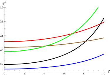
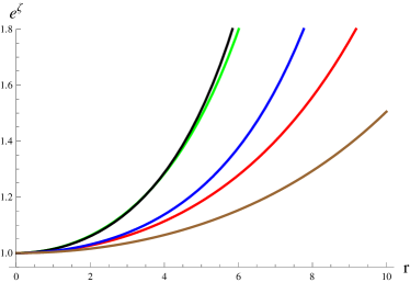
Figure 1: Metric potentials versus $r$ for different compact star candidates

This section is related to the study of various physical characteristics of the considered compact stars associated with anisotropic distribution in their interiors in the framework of $f(\mathcal{R},\mathcal{T},\mathcal{R}_{\omega\alpha}\mathcal{T}^{\omega\alpha})$ theory. We analyze the graphical behavior of both developed solutions (23)-(25) and (26)-(28) for $\varpi=\pm 4$ corresponding to all stars by using their respective preliminary data provided in Tables $\mathbf{1}$ and $\mathbf{2}$. Further, we check the physical behavior of temporal as well as radial metric functions, anisotropy, energy conditions and mass in the interior of all quark candidates. For particular values of the model parameter, we also analyze the stability of resulting solutions. It is familiar that the resulting solution will be assumed compatible if the metric potential possesses non-singular and increasing nature in the whole positive domain. In this case, the metric coefficients are presented in Eqs.(33) and (34) involving four constants which are calculated in Table $\mathbf{2}$. Figure $\mathbf{1}$ exhibits their plots from which we observe that our resulting solutions are physically consistent. It is worth mentioning here that the brown color expresses Cen X-3 compact star, blue indicates 4U 1820-30, red signifies Her X-I, black represents SAX J 1808.4-3658 and green color shows RXJ 1856-37 in all plots.

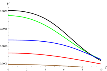
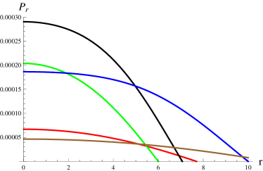
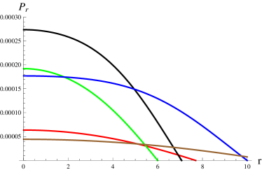
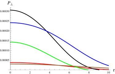
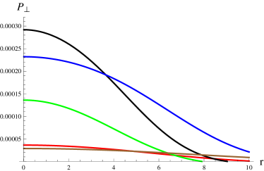
Figure 2: Plots of energy density, radial pressure and tangential pressure versus $r$ corresponding to $\varpi=4$ and $\mathbb{L}_{m}=-\mu$ (left) as well as $\mathbb{L}_{m}=P_{r}$ (right) for different compact star candidates

4.1 Study of Physical Variables and their Regularity Conditions

The physically acceptable solution guarantees the maximum value of matter variables like energy density and pressure at the center and minimum value at the boundary of self-gravitating stellar structures. Figure $\mathbf{2}$ assures that $\varpi=4$ provides acceptable solutions corresponding to each star for both choices of matter Lagrangian, as all variables fulfill the above acceptability criteria, thus these compact stars have extremely dense structures in modified gravity. Figure $\mathbf{2}$ (two plots in second row) also show the disappearance of radial pressure at the surface of each candidate. In Tables $\mathbf{3}$ and $\mathbf{4}$, the calculated values of $\mu_{c},~{}\mu_{s}$ and $P_{rc}$ are provided with respect to both solutions, which indicate the energy density at center, at surface and radial pressure at center, respectively. We can see from these tables that the solution corresponding to $\mathbb{L}_{m}=-\mu$ provides more dense structure of each star. To show regular behavior of the solution, some conditions at the center should be satisfied as $\frac{d\mu}{dr}|_{r=0}=0,~{}\frac{dP_{r}}{dr}|_{r=0}=0,~{}\frac{d^{2}\mu}{dr^{2}}|_{r=0}<0$ and $\frac{d^{2}P_{r}}{dr^{2}}|_{r=0}<0$. Figures $\mathbf{3}$ and $\mathbf{4}$ reveal that both solutions fulfill maximality conditions.

The graphical nature of the matter variables and their differentials corresponding to both the obtained solutions is also checked for $\varpi=-4$ and found to be acceptable, but their graphs are not added in this article.

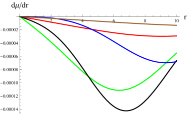
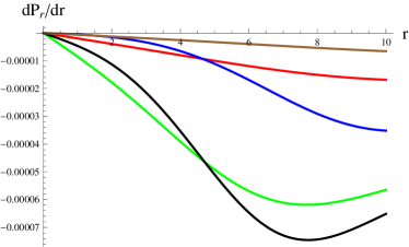
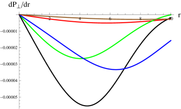
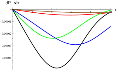
Figure 3: Plots of $\frac{d\mu}{dr},~{}\frac{dP_{r}}{dr}$ and $\frac{dP_{\bot}}{dr}$ versus $r$ corresponding to $\varpi=4$ and $\mathbb{L}_{m}=-\mu$ (left) as well as $\mathbb{L}_{m}=P_{r}$ (right) for different compact star candidates

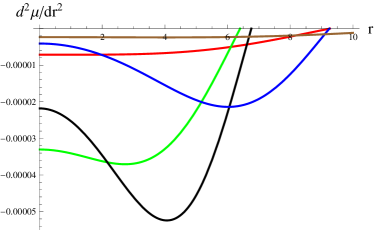
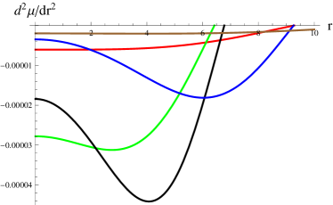
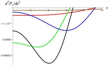
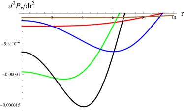
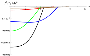
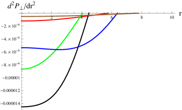
Figure 4: Plots of $\frac{d^{2}\mu}{dr^{2}},~{}\frac{d^{2}P_{r}}{dr^{2}}$ and $\frac{d^{2}P_{\bot}}{dr^{2}}$ versus $r$ corresponding to $\varpi=4$ and $\mathbb{L}_{m}=-\mu$ (left) as well as $\mathbb{L}_{m}=P_{r}$ (right) for different compact star candidates

4.2 Effect of Anisotropic Pressure

For the first solution corresponding to $\mathbb{L}_{m}=-\mu$, the anisotropy (i.e., $\Delta=P_{\bot}-P_{r}$) is obtained as

$$\Delta =\bigg{[}2\big{(}\varpi W\big{(}-Ze^{2r^{2}W}+2r^{2}W+3\big{)}+4\pi\big{(}r^{2}WZe^{2r^{2}W}+1\big{)}^{2}\big{)}\big{(}32\pi\big{(}r^{2}WZ$$

$$\times e^{2r^{2}W}+1\big{)}^{3}-\varpi W\big{(}2r^{2}W\big{(}14Z^{2}e^{4r^{2}W}+Ze^{2r^{2}W}-6\big{)}+25Ze^{2r^{2}W}+32$$

$$\times r^{6}W^{3}Z^{2}e^{4r^{2}W}+4r^{4}W^{2}Ze^{2r^{2}W}\big{(}Z^{2}e^{4r^{2}W}+8Ze^{2r^{2}W}+6\big{)}-34\big{)}\big{)}\bigg{]}^{-1}\bigg{[}256$$

$$\times\pi^{2}\mathfrak{B_{c}}\big{(}r^{2}WZe^{2r^{2}W}+1\big{)}^{5}-16\pi W\big{(}r^{2}WZe^{2r^{2}W}+1\big{)}^{2}\big{(}-28\varpi\mathfrak{B_{c}}+r^{2}W$$

$$\times\big{(}Ze^{2r^{2}W}-2\big{)}\big{(}8\varpi\mathfrak{B_{c}}+3Z(8\varpi\mathfrak{B_{c}}+1)e^{2r^{2}W}+4\big{)}+3Z(4\varpi\mathfrak{B_{c}}+1)e^{2r^{2}W}$$

$$+32\varpi\mathfrak{B_{c}}r^{6}W^{3}Z^{2}e^{4r^{2}W}+2r^{4}W^{2}Ze^{2r^{2}W}\big{(}-4(3\varpi\mathfrak{B_{c}}+1)+\varpi\mathfrak{B_{c}}Z^{2}e^{4r^{2}W}$$

$$+2Z(7\varpi\mathfrak{B_{c}}+1)e^{2r^{2}W}\big{)}-6\big{)}+\varpi W^{2}\big{(}8(25\varpi\mathfrak{B_{c}}+16)+Z^{2}(24\varpi\mathfrak{B_{c}}+19)$$

$$\times e^{4r^{2}W}+2r^{2}W\big{(}4(44\varpi\mathfrak{B_{c}}+31)+2Z^{3}(25\varpi\mathfrak{B_{c}}+8)e^{6r^{2}W}-Z^{2}(240\varpi\mathfrak{B_{c}}$$

$$+83)e^{4r^{2}W}-4Z(25\varpi\mathfrak{B_{c}}+23)e^{2r^{2}W}\big{)}-50Z(4\varpi\mathfrak{B_{c}}+3)e^{2r^{2}W}+384\varpi\mathfrak{B_{c}}$$

$$\times r^{10}W^{5}Z^{3}e^{6r^{2}W}-32r^{8}W^{4}Z^{2}e^{4r^{2}W}\big{(}10\varpi\mathfrak{B_{c}}+\varpi\mathfrak{B_{c}}Z^{2}e^{4r^{2}W}-2Z(4\varpi\mathfrak{B_{c}}$$

$$+3)e^{2r^{2}W}+4\big{)}-8r^{6}W^{3}Ze^{2r^{2}W}\big{(}-16\varpi\mathfrak{B_{c}}+3\varpi\mathfrak{B_{c}}Z^{3}e^{6r^{2}W}-Z^{2}(33\varpi\mathfrak{B_{c}}$$

$$+10)e^{4r^{2}W}+220\varpi\mathfrak{B_{c}}Ze^{2r^{2}W}+12\big{)}+4r^{4}W^{2}\big{(}72\varpi\mathfrak{B_{c}}+Z^{4}(2\varpi\mathfrak{B_{c}}+1)$$

$$\times e^{8r^{2}W}+Z^{3}(43\varpi\mathfrak{B_{c}}+9)e^{6r^{2}W}-2Z^{2}(166\varpi\mathfrak{B_{c}}+41)e^{4r^{2}W}-2Z(38\varpi\mathfrak{B_{c}}$$

$$-13)e^{2r^{2}W}+12\big{)}\big{)}\bigg{]},$$ (45)

and the solution for $\mathbb{L}_{m}=P_{r}$ yields

$$\Delta =\bigg{[}2\big{(}4\pi\big{(}r^{2}WZe^{2r^{2}W}+1\big{)}^{2}+\varpi W\big{(}-Ze^{2r^{2}W}+4r^{2}W+2r^{4}W^{2}Ze^{2r^{2}W}$$

$$+3\big{)}\big{)}\big{(}32\pi\big{(}r^{2}WZe^{2r^{2}W}+1\big{)}^{3}-\varpi W\big{(}2r^{2}W\big{(}10Z^{2}e^{4r^{2}W}-23Ze^{2r^{2}W}-6\big{)}$$

$$+17Ze^{2r^{2}W}+32r^{6}W^{3}Z^{2}e^{4r^{2}W}+4r^{4}W^{2}Ze^{2r^{2}W}\big{(}Z^{2}e^{4r^{2}W}+6\big{)}-50\big{)}\big{)}\bigg{]}^{-1}$$

$$\times\bigg{[}256\pi^{2}\mathfrak{B_{c}}\big{(}r^{2}WZe^{2r^{2}W}+1\big{)}^{5}-16\pi W\big{(}r^{2}WZe^{2r^{2}W}+1\big{)}^{2}\big{(}-6(6\varpi\mathfrak{B_{c}}$$

$$+1)+r^{2}W\big{(}-8(3\varpi\mathfrak{B_{c}}+1)+Z^{2}(20\varpi\mathfrak{B_{c}}+3)e^{4r^{2}W}-2Z(32\varpi\mathfrak{B_{c}}+1)$$

$$\times e^{2r^{2}W}\big{)}+Z(8\varpi\mathfrak{B_{c}}+3)e^{2r^{2}W}+24\varpi\mathfrak{B_{c}}r^{6}W^{3}Z^{2}e^{4r^{2}W}+2r^{4}W^{2}Ze^{2r^{2}W}$$

$$\times\big{(}-4(5\varpi\mathfrak{B_{c}}+1)+\varpi\mathfrak{B_{c}}Z^{2}e^{4r^{2}W}+2Z(3\varpi\mathfrak{B_{c}}+1)e^{2r^{2}W}\big{)}\big{)}+\varpi W^{2}\big{(}(33$$

$$\times\varpi\mathfrak{B_{c}}+16)8+Z^{2}(12\varpi\mathfrak{B_{c}}+19)e^{4r^{2}W}+2r^{2}W\big{(}4(56\varpi\mathfrak{B_{c}}+29)+2Z^{3}$$

$$\times(19\varpi\mathfrak{B_{c}}+8)e^{6r^{2}W}-Z^{2}(216\varpi\mathfrak{B_{c}}+83)e^{4r^{2}W}+8Z(55\varpi\mathfrak{B_{c}}-12)e^{2r^{2}W}\big{)}$$

$$-30Z(2\varpi\mathfrak{B_{c}}+5)e^{2r^{2}W}+128\varpi\mathfrak{B_{c}}r^{10}W^{5}Z^{3}e^{6r^{2}W}+16r^{8}W^{4}Z^{2}e^{4r^{2}W}\big{(}\varpi\mathfrak{B_{c}}$$

$$\times Z^{2}e^{4r^{2}W}-48\varpi\mathfrak{B_{c}}+10Ze^{2r^{2}W}-8\big{)}+8r^{6}W^{3}Ze^{2r^{2}W}\big{(}-4(4\varpi\mathfrak{B_{c}}+3)$$

$$+5\varpi\mathfrak{B_{c}}Z^{3}e^{6r^{2}W}+Z^{2}(4\varpi\mathfrak{B_{c}}+9)e^{4r^{2}W}-2Z(46\varpi\mathfrak{B_{c}}+5)e^{2r^{2}W}\big{)}+4r^{4}W^{2}$$

$$\times\big{(}24\varpi\mathfrak{B_{c}}+Z^{4}(6\varpi\mathfrak{B_{c}}+1)e^{8r^{2}W}-Z^{3}(2\varpi\mathfrak{B_{c}}-9)e^{6r^{2}W}-2Z^{2}(44\varpi\mathfrak{B_{c}}$$

$$+43)e^{4r^{2}W}+10Z(26\varpi\mathfrak{B_{c}}+1)e^{2r^{2}W}+12\big{)}\big{)}\bigg{]}.$$ (46)

We utilize the experimental data (Table $\mathbf{1}$) and calculated constants (Table $\mathbf{2}$) to check the role of pressure anisotropy in the development of compact structures. The anisotropy shows increasing (outward) or decreasing (inward) behavior depending on whether the tangential pressure is greater or lesser than the radial pressure, respectively. Figure $\mathbf{5}$ (upper two plots) shows that anisotropy in the interior of Cen X-3, Her X-I and RXJ 1856-37 stars varies from negative to positive, while it exhibits decreasing behavior near the center and then increases towards boundary inside 4U 1820-30 and 1808.4-3658 stars. This factor shows same behavior for both values of $\varpi$.

According to Hossain et al. [75], negative anisotropy allows the construction of massive stellar structure. It is prominent from the graphical interpretation that anisotropy will become positive after overcoming the negative value. The positive anisotropy helps to construct the more compact object, according to Gokhroo and Mehra [76]. Also, we can see that the anisotropy increases and attains its maximum value at the boundary of each star candidate which is an inherent property of an ultra dense compact stars [77].

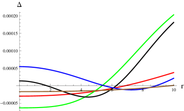
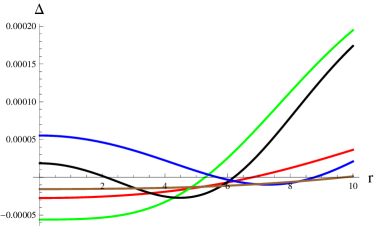
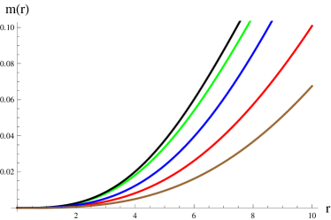
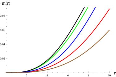
Figure 5: Variation of anisotropy and mass versus $r$ corresponding to $\varpi=4$ and $\mathbb{L}_{m}=-\mu$ (left) as well as $\mathbb{L}_{m}=P_{r}$ (right) for different compact star candidates

4.3 Effective Mass, Compactness and Surface Redshift

The effective mass of spherical geometry can be defined as

$$m(r)=\frac{1}{2}\int_{0}^{\mathcal{H}}r^{2}\mu dr,$$ (47)

or it can be derived from Eq.(19) as

$$m(r)=\frac{r}{2}\left\{\frac{2\bar{M}r^{2}e^{\frac{\bar{M}\left(\mathcal{H}^{2}-r^{2}\right)}{\mathcal{H}^{2}(2\bar{M}-\mathcal{H})}}}{2\bar{M}r^{2}e^{\frac{\bar{M}\left(\mathcal{H}^{2}-r^{2}\right)}{\mathcal{H}^{2}(2\bar{M}-\mathcal{H})}}+\mathcal{H}^{2}(\mathcal{H}-2\bar{M})}\right\},$$ (48)

which shows that there is no mass at the center of each strange star. Figure $\mathbf{5}$ (second row) contains the plots of mass for both solutions which show that compact objects become more massive for the first solution corresponding to $\mathbb{L}_{m}=-\mu$. The evolution of massive bodies can be studied by investigating various physical quantities, i.e., the compactness factor which is defined as the mass to radius ratio of a compact star. Its mathematical expression is given as

$$\sigma(r)=\frac{m(r)}{r}=\frac{1}{2}\left\{\frac{2\bar{M}r^{2}e^{\frac{\bar{M}\left(\mathcal{H}^{2}-r^{2}\right)}{\mathcal{H}^{2}(2\bar{M}-\mathcal{H})}}}{2\bar{M}r^{2}e^{\frac{\bar{M}\left(\mathcal{H}^{2}-r^{2}\right)}{\mathcal{H}^{2}(2\bar{M}-\mathcal{H})}}+\mathcal{H}^{2}(\mathcal{H}-2\bar{M})}\right\},$$ (49)

whose maximum value for a feasible solution corresponding to a self-gravitating body has been found by Buchdahl [72] after matching the interior and exterior regions of spacetimes at hypersurface ($r=\mathcal{H}$) as $\frac{4}{9}$. The measurement of wavelength of electromagnetic radiations emitting from a massive object with enough gravitational attraction is known as redshift, given as

$$D(r)=\frac{1}{\sqrt{1-2\sigma(r)}}-1,$$ (50)

which further becomes

$$D(r)=-1+\sqrt{\frac{2\bar{M}r^{2}e^{\frac{\bar{M}\left(\mathcal{H}^{2}-r^{2}\right)}{\mathcal{H}^{2}(2\bar{M}-\mathcal{H})}}+\mathcal{H}^{2}(\mathcal{H}-2\bar{M})}{\mathcal{H}^{2}(\mathcal{H}-2\bar{M})}}.$$ (51)

Buchdahl proposed its upper limit inside a feasible compact star having perfect fluid as $2$, while it was observed to be $5.211$ [78] for anisotropic configured structures. Figure $\mathbf{6}$ shows the plots of these factors with respect to each star for both solutions and we find them consistent with their respective limits for $\varpi=4$ (Tables $\mathbf{3}$ and $\mathbf{4}$). It is seen that increment in the value of bag constant increases the above factors. The behavior of mass, compactness and redshift meets their respective acceptability criteria for $\varpi=-4$ as well.

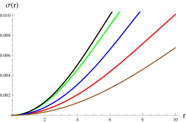
Figure 6: Variation of compactness and redshift factors versus $r$ corresponding to $\varpi=4$ and $\mathbb{L}_{m}=-\mu$ (left) as well as $\mathbb{L}_{m}=P_{r}$ (right) for different compact star candidates

4.4 Energy Conditions

Various constrains involving the state variables (and charge in the presence of electromagnetic field) have widely been used in astrophysics to ensure whether the matter in a particular geometry is normal or exotic. The fulfilment of such bounds also guarantee viability of the resulting solution. A realistic configuration is the one which satisfies all the following constraints

• Null: $\mu+P_{r}\geq 0$,  $\mu+P_{\bot}\geq 0$,

• Weak: $\mu\geq 0$,  $\mu+P_{r}\geq 0$,  $\mu+P_{\bot}\geq 0$,

• Strong: $\mu+P_{r}+2P_{\bot}\geq 0$,

• Dominant: $\mu-P_{r}\geq 0$,  $\mu-P_{\bot}\geq 0$.

The graphical analysis of the above conditions for both resulting solutions is presented in Figures $\mathbf{7}$ and $\mathbf{8}$, from which it is observed that our developed solutions as well as $f(\mathcal{R},\mathcal{T},\mathcal{Q})$ model (8) are physically viable for $\varpi=4$. We also check these conditions with respect to $\varpi=-4$ and obtain viable results, but their graphs have not been added. Thus it can be doubtlessly said that there must exist normal matter in the interior of all quark candidates.

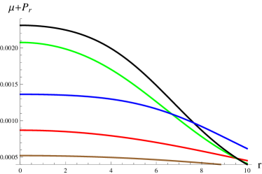
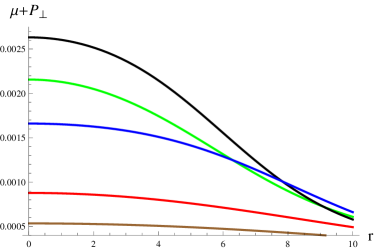
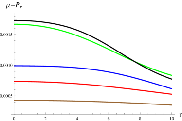
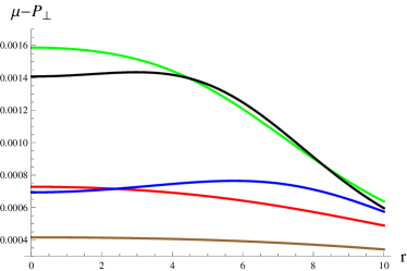
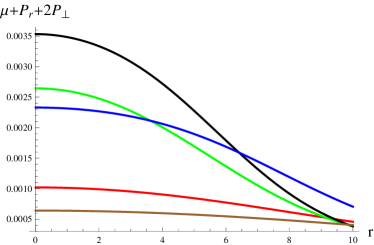
Figure 7: Plots of energy conditions versus $r$ corresponding to $\varpi=4$ and $\mathbb{L}_{m}=-\mu$ for different compact star candidates

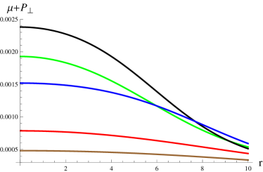
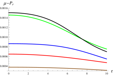
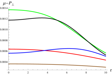
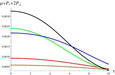
Figure 8: Plots of energy conditions versus $r$ corresponding to $\varpi=4$ and $\mathbb{L}_{m}=P_{r}$ for different compact star candidates

4.5 Stability Analysis

The stability of physical models and astronomical objects gained much attention in explaining different phases of our cosmos. One can get better understanding about the structural evolution of compact bodies which meet the stability criteria. In this regard, various approaches have been discussed in literature such as causality condition and adiabatic index etc. We utilize these techniques to analyze the stability of quark candidates for the model (8). According to the causality condition [79], the speed of light must be greater than the speed of sound within a stable system, i.e., $0<v_{sr}^{2}<1$ and $0<v_{s\bot}^{2}<1$. Here, $v_{sr}$ and $v_{s\bot}$ are sound speeds in radial and tangential directions, respectively and expressed as

$$v_{sr}^{2}=\frac{dP_{r}}{d\mu},\quad v_{s\bot}^{2}=\frac{dP_{\bot}}{d\mu}.$$ (52)

The stability can also be checked with the help of Herrera’s cracking concept [39] which states that stable structure must satisfy the inequality $0<\mid v_{s\bot}^{2}-v_{sr}^{2}\mid<1$ in its interior. The gravitational cracking happens when the radial force is directed inwards in the inner part of the sphere for all values of the radial coordinate $r$ between the center, and some value beyond which the force reverses its direction.

Another powerful approach which helps to analyze the stability of self-gravitating structure is the adiabatic index $\big{(}\Gamma\big{)}$. Many researchers [80, 81] utilized this tool to study celestial bodies and concluded that its value should not be less than $\frac{4}{3}$ everywhere in stable models. The mathematical representation of $\Gamma$ is

$$\Gamma=\frac{\mu+P_{r}}{P_{r}}\left(\frac{dP_{r}}{d\mu}\right)=\frac{\mu+P_{r}}{P_{r}}\left(v_{sr}^{2}\right).$$ (53)

Figure $\mathbf{9}$ depicts the graphs of $\mid v_{s\bot}^{2}-v_{sr}^{2}\mid$ and $\Gamma$ for each quark star corresponding to both solutions for $\varpi=4$. The upper left plot shows that all stars are stable everywhere except 4U 1820-30 (which is unstable near its core and stable towards boundary) with respect to the solution for $\mathbb{L}_{m}=-\mu$, while the solution corresponding to $\mathbb{L}_{m}=P_{r}$ provides that two stars, namely 4U 1820-30 and SAX J 1808.4-3658 are unstable near their center (upper right plot).

As $\varpi=-4$ is concerned, the stability of the solution corresponding to $\mathbb{L}_{m}=-\mu$ produces same results as we have obtained for $\varpi=4$. On the contrary, the interior of the compact star SAX J 1808.4-3658 is stable throughout corresponding to the solution with respect to $\mathbb{L}_{m}=P_{r}$, as shown in Figure $\mathbf{10}$. The adiabatic index is found to be within its acceptable range for both the cases (lower plots of Figures $\mathbf{9}$ and $\mathbf{10}$).

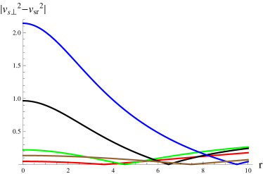
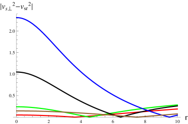
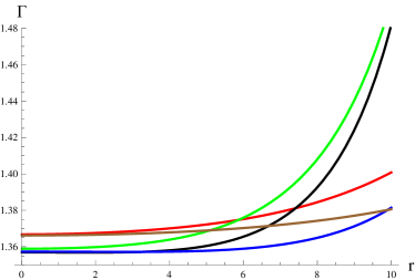
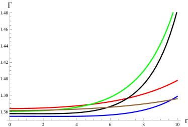
Figure 9: Plots of $\mid v_{s\bot}^{2}-v_{sr}^{2}\mid$ and adiabatic index versus $r$ corresponding to $\varpi=4$ and $\mathbb{L}_{m}=-\mu$ (left) as well as $\mathbb{L}_{m}=P_{r}$ (right) for different compact star candidates

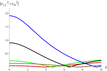
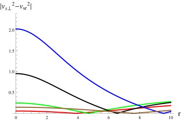
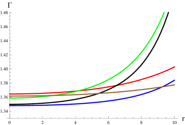
Figure 10: Plots of $\mid v_{s\bot}^{2}-v_{sr}^{2}\mid$ and adiabatic index versus $r$ corresponding to $\varpi=-4$ and $\mathbb{L}_{m}=-\mu$ (left) as well as $\mathbb{L}_{m}=P_{r}$ (right) for different compact star candidates

5 Final Remarks

This paper explores the existence of anisotropic stars in the framework of $f(\mathcal{R},\mathcal{T},\mathcal{R}_{\omega\alpha}\mathcal{T}^{\omega\alpha})$ gravity. We have taken a linear model $\mathcal{R}+\varpi\mathcal{R}_{\omega\alpha}\mathcal{T}^{\omega\alpha}$ which still upholds the matter-geometry coupling effects in the interior of compact stars, where the coupling constant $\varpi$ has been chosen as $\pm 4$. The modified field equations and $\mathbb{TOV}$ equation have been formulated for the above model with respect to two different choices of matter Lagrangian. We have adopted an acceptable temporal metric function [53, 54] and utilized embedding class-one condition to calculate radial metric potential (34) and found a solution to the field equations. We have also assumed $\mathbb{MIT}$ bag model $\mathbb{E}$o$\mathbb{S}$ which interconnects the energy density and radial pressure of the inner configuration. Both metric coefficients involve four unknowns ($W,X,Y,Z$) whose values have been calculated at the boundary in terms of mass and radius of celestial body. The observational data of five different strange stars, i.e., 4U 1820-30, Cen X-3, RXJ 1856-37, SAX J 1808.4-3658 and Her X-I (Table $\mathbf{1}$) have been employed to calculate unknown quantities (Table $\mathbf{2}$) and bag constant with respect to each candidate. Tables $\mathbf{3}$ and $\mathbf{4}$ contain the values of energy density (at center and surface), radial pressure (at center), compactness as well as redshift (at surface) and bag constant for both solutions. Figure $\mathbf{5}$ shows that mass of each quark body decreases by decreasing the bag constant. The graphical interpretation of matter variables has also been analyzed. It is found that the state variables corresponding to both solutions show physically acceptable behavior as they are maximum at the center and minimum at the boundary of respective star candidate.

The interior of all stars become more dense for the solution corresponding to $\mathbb{L}_{m}=-\mu$, whereas $\mathbb{L}_{m}=P_{r}$ provides less dense structures. We have found acceptable behavior of redshift and compactness (Figure $\mathbf{6}$). The positive behavior of energy bounds confirmed the viability of both developed solutions as well as presence of normal matter in the interior of stellar bodies (Figures $\mathbf{7}$ and $\mathbf{8}$). Finally, we have utilized two approaches to check the stability of resulting solutions for $\varpi=\pm 4$. The first one is the Herrera’s cracking approach which guarantees the fulfilment of the inequality $0<\mid v_{s\bot}^{2}-v_{sr}^{2}\mid<1$ within stable system. All candidate stars are observed to be stable except 4U 1820-30 (which is unstable near its core) for the solution corresponding to $\mathbb{L}_{m}=-\mu$ (upper left plot of Figures $\mathbf{9}$ and $\mathbf{10}$), while for $\mathbb{L}_{m}=P_{r}$ and $\varpi=4$, stars 4U 1820-30 and SAX J 1808.4-3658 become unstable near their center and show stable behavior towards the boundary (upper right plot of Figure $\mathbf{9}$). However, the compact candidate SAX J 1808.4-3658 is observed to be stable throughout for the solution with respect to $\mathbb{L}_{m}=P_{r}$ and $\varpi=-4$ (upper right plot of Figure $\mathbf{10}$). The other three stars, namely Cen X-3, Her X-I and RXJ 1856-37 are found to be stable with respect to each solution. Figures $\mathbf{9}$ and $\mathbf{10}$ (lower plots) show the behavior of adiabatic index which provides acceptable values everywhere.

In the framework of $\mathbb{GR}$, the central density, surface density as well as central radial pressure corresponding to two different stars, namely Her X-1 and RXJ 1856-37 have been calculated [53]. By comparing our results, we observe that these physical quantities have less values in this modified gravity. The values of physical variables inside the quark star SAX J 1808.4-3658 have been determined in $f(\mathcal{R},\mathcal{T})$ theory [49], from which we have found that the internal configuration of this star becomes more dense in $f(\mathcal{R},\mathcal{T},\mathcal{Q})$. The interior of the star candidate 4U 1820-30 in this theory is found to be less dense than that in $f(\mathcal{G})$ gravity [62]. For $\varpi=-4$, we obtain more suitable results in $f(\mathcal{R},\mathcal{T},\mathcal{R}_{\omega\alpha}\mathcal{T}^{\omega\alpha})$ theory as compared to [25] as well as the solution corresponding to $\varpi=4$. Finally, one can reduce all these results to $\mathbb{GR}$ by taking $\varpi=0$ in the modified model (8).

Appendix A

The state variables (23)-(25) in terms of unknowns $(W,X,Y,Z)$ take the form

$$\mu =\bigg{[}32\pi\big{(}r^{2}WZe^{2r^{2}W}+1\big{)}^{3}-\varpi W\big{\{}2r^{2}W\big{(}14Z^{2}e^{4r^{2}W}+Ze^{2r^{2}W}-6\big{)}+25Z$$

$$\times e^{2r^{2}W}+32r^{6}W^{3}Z^{2}e^{4r^{2}W}+4r^{4}W^{2}Ze^{2r^{2}W}\big{(}Z^{2}e^{4r^{2}W}+8Ze^{2r^{2}W}+6\big{)}-34\big{\}}\bigg{]}^{-1}$$

$$\times\bigg{[}32\pi\mathfrak{B_{c}}+2r^{2}W^{2}\big{(}24\varpi\mathfrak{B_{c}}+Z^{2}e^{4r^{2}W}\big{(}-20\varpi\mathfrak{B_{c}}+48\pi\mathfrak{B_{c}}r^{2}+3\big{)}-2Z$$

$$\times(14\varpi\mathfrak{B_{c}}-9)e^{2r^{2}W}\big{)}+2W\big{(}20\varpi\mathfrak{B_{c}}+Ze^{2r^{2}W}\big{(}-20\varpi\mathfrak{B_{c}}+48\pi\mathfrak{B_{c}}r^{2}+3\big{)}$$

$$+6\big{)}-32\varpi\mathfrak{B_{c}}r^{6}W^{4}Z^{2}e^{4r^{2}W}+4r^{4}W^{3}Z^{2}e^{4r^{2}W}\big{(}-20\varpi\mathfrak{B_{c}}+\mathfrak{B_{c}}Z\big{(}8\pi r^{2}-\varpi\big{)}$$

$$\times e^{2r^{2}W}+6\big{)}\bigg{]},$$

$$P_{r} =\bigg{[}32\pi\big{(}r^{2}WZe^{2r^{2}W}+1\big{)}^{3}-\varpi W\big{\{}2r^{2}W\big{(}14Z^{2}e^{4r^{2}W}+Ze^{2r^{2}W}-6\big{)}+25Z$$

$$\times e^{2r^{2}W}+32r^{6}W^{3}Z^{2}e^{4r^{2}W}+4r^{4}W^{2}Ze^{2r^{2}W}\big{(}Z^{2}e^{4r^{2}W}+8Ze^{2r^{2}W}+6\big{)}-34\big{\}}\bigg{]}^{-1}$$

$$\times\bigg{[}-2\big{(}r^{2}WZe^{2r^{2}W}+1\big{)}\big{(}16\pi\mathfrak{B_{c}}+2r^{2}W^{2}Ze^{2r^{2}W}\big{(}-4\varpi\mathfrak{B_{c}}+\big{(}8\pi r^{2}-\varpi\big{)}$$

$$\mathfrak{B_{c}}Ze^{2r^{2}W}-2\big{)}+W\big{(}16\varpi\mathfrak{B_{c}}+Ze^{2r^{2}W}\big{(}-10\varpi\mathfrak{B_{c}}+32\pi\mathfrak{B_{c}}r^{2}-1\big{)}-2\big{)}-16$$

$$\times\varpi\mathfrak{B_{c}}r^{4}W^{3}Ze^{2r^{2}W}\big{)}\bigg{]},$$

$$P_{\bot} =\bigg{[}2\big{\{}\varpi W\big{(}-Ze^{2r^{2}W}+2r^{2}W+3\big{)}+4\pi\big{(}r^{2}WZe^{2r^{2}W}+1\big{)}^{2}\big{\}}\big{\{}32\pi\big{(}r^{2}WZe^{2r^{2}W}$$

$$+1\big{)}^{3}-\varpi W\big{(}2r^{2}W\big{(}14Z^{2}e^{4r^{2}W}+Ze^{2r^{2}W}-6\big{)}+25Ze^{2r^{2}W}+32r^{6}W^{3}Z^{2}e^{4r^{2}W}$$

$$+4r^{4}W^{2}Ze^{2r^{2}W}\big{(}Z^{2}e^{4r^{2}W}+8Ze^{2r^{2}W}+6\big{)}-34\big{)}\big{\}}\bigg{]}^{-1}\bigg{[}W\big{\{}\varpi W\big{(}8(\varpi\mathfrak{B_{c}}+19)$$

$$-Z^{2}(16\varpi\mathfrak{B_{c}}-15)e^{4r^{2}W}+2r^{2}W\big{(}4(28\varpi\mathfrak{B_{c}}+33)+2Z^{3}(13\varpi\mathfrak{B_{c}}+7)e^{6r^{2}W}$$

$$-Z^{2}(152\varpi\mathfrak{B_{c}}+89)e^{4r^{2}W}-4Z(27\varpi\mathfrak{B_{c}}+13)e^{2r^{2}W}\big{)}-2Z(8\varpi\mathfrak{B_{c}}+73)e^{2r^{2}W}$$

$$+384\varpi\mathfrak{B_{c}}r^{10}W^{5}Z^{3}e^{6r^{2}W}-32r^{8}W^{4}Z^{2}e^{4r^{2}W}\big{(}6\varpi\mathfrak{B_{c}}+\varpi\mathfrak{B_{c}}Z^{2}e^{4r^{2}W}-2Z(4\varpi\mathfrak{B_{c}}$$

$$+3)e^{2r^{2}W}+4\big{)}-8r^{6}W^{3}Ze^{2r^{2}W}\big{(}-32\varpi\mathfrak{B_{c}}+3\varpi\mathfrak{B_{c}}Z^{3}e^{6r^{2}W}-Z^{2}(27\varpi\mathfrak{B_{c}}+10)$$

$$\times e^{4r^{2}W}+4Z(47\varpi\mathfrak{B_{c}}-1)e^{2r^{2}W}+12\big{)}+4r^{4}W^{2}\big{(}72\varpi\mathfrak{B_{c}}+Z^{4}e^{8r^{2}W}+Z^{3}e^{6r^{2}W}$$

$$(41\varpi\mathfrak{B_{c}}+5)-4Z^{2}(75\varpi\mathfrak{B_{c}}+17)e^{4r^{2}W}-2Z(22\varpi\mathfrak{B_{c}}-19)e^{2r^{2}W}+12\big{)}\big{)}-32\pi$$

$$\times\big{(}r^{2}WZe^{2r^{2}W}+1\big{)}^{2}\big{(}r^{2}W\big{(}-4(\varpi\mathfrak{B_{c}}+1)+Z^{2}(4\varpi\mathfrak{B_{c}}+1)e^{4r^{2}W}-2Ze^{2r^{2}W}$$

$$\times(5\varpi\mathfrak{B_{c}}+2)\big{)}+e^{2r^{2}W}(Z-\varpi\mathfrak{B_{c}}Z)+8\varpi\mathfrak{B_{c}}r^{6}W^{3}Z^{2}e^{4r^{2}W}+2r^{4}W^{2}Ze^{2r^{2}W}$$

$$\times\big{(}\varpi\mathfrak{B_{c}}\big{(}5Ze^{2r^{2}W}-8\big{)}-2\big{)}-4\big{)}\big{\}}\bigg{]},$$

and Eqs.(26)-(28) become

$$\mu =\bigg{[}32\pi\big{(}r^{2}WZe^{2r^{2}W}+1\big{)}^{3}-\varpi W\big{\{}2r^{2}W\big{(}10Z^{2}e^{4r^{2}W}-23Ze^{2r^{2}W}-6\big{)}+17Z$$

$$\times e^{2r^{2}W}+32r^{6}W^{3}Z^{2}e^{4r^{2}W}+4r^{4}W^{2}Ze^{2r^{2}W}\big{(}Z^{2}e^{4r^{2}W}+6\big{)}-50\big{\}}\bigg{]}^{-1}\bigg{[}32\pi\mathfrak{B_{c}}$$

$$+2r^{2}W^{2}\big{(}24\varpi\mathfrak{B_{c}}+Z^{2}e^{4r^{2}W}\big{(}-16\varpi\mathfrak{B_{c}}+48\pi\mathfrak{B_{c}}r^{2}+3\big{)}-2Z(2\varpi\mathfrak{B_{c}}-9)e^{2r^{2}W}\big{)}$$

$$+2W\big{(}28\varpi\mathfrak{B_{c}}+Ze^{2r^{2}W}\big{(}-16\varpi\mathfrak{B_{c}}+48\pi\mathfrak{B_{c}}r^{2}+3\big{)}+6\big{)}-32\varpi\mathfrak{B_{c}}r^{6}W^{4}Z^{2}e^{4r^{2}W}$$

$$+4r^{4}W^{3}Z^{2}e^{4r^{2}W}\big{(}-12\varpi\mathfrak{B_{c}}+\mathfrak{B_{c}}Z\big{(}8\pi r^{2}-\varpi\big{)}e^{2r^{2}W}+6\big{)}\bigg{]},$$

$$P_{r} =\bigg{[}32\pi\big{(}r^{2}WZe^{2r^{2}W}+1\big{)}^{3}-\varpi W\big{\{}2r^{2}W\big{(}10Z^{2}e^{4r^{2}W}-23Ze^{2r^{2}W}-6\big{)}+17Z$$

$$\times e^{2r^{2}W}+32r^{6}W^{3}Z^{2}e^{4r^{2}W}+4r^{4}W^{2}Ze^{2r^{2}W}\big{(}Z^{2}e^{4r^{2}W}+6\big{)}-50\big{\}}\bigg{]}^{-1}\bigg{[}-2\big{(}r^{2}$$

$$\times WZe^{2r^{2}W}+1\big{)}\big{(}16\pi\mathfrak{B_{c}}+2r^{2}W^{2}Ze^{2r^{2}W}\big{(}4\varpi\mathfrak{B_{c}}+\mathfrak{B_{c}}Z\big{(}8\pi r^{2}-\varpi\big{)}e^{2r^{2}W}-2\big{)}$$

$$+W\big{(}24\varpi\mathfrak{B_{c}}+Ze^{2r^{2}W}\big{(}-6\varpi\mathfrak{B_{c}}+32\pi\mathfrak{B_{c}}r^{2}-1\big{)}-2\big{)}-16\varpi\mathfrak{B_{c}}r^{4}W^{3}Ze^{2r^{2}W}\big{)}\bigg{]},$$

$$P_{\bot} =\bigg{[}2\big{\{}4\pi\big{(}r^{2}WZe^{2r^{2}W}+1\big{)}^{2}+\varpi W\big{(}-Ze^{2r^{2}W}+4r^{2}W+2r^{4}W^{2}Ze^{2r^{2}W}+3\big{)}\big{\}}$$

$$\times\big{\{}32\pi\big{(}r^{2}WZe^{2r^{2}W}+1\big{)}^{3}-\varpi W\big{(}2r^{2}W\big{(}10Z^{2}e^{4r^{2}W}-23Ze^{2r^{2}W}-6\big{)}+17Ze^{2r^{2}W}$$

$$+32r^{6}W^{3}Z^{2}e^{4r^{2}W}+4r^{4}W^{2}Ze^{2r^{2}W}\big{(}Z^{2}e^{4r^{2}W}+6\big{)}-50\big{)}\big{\}}\bigg{]}^{-1}\bigg{[}W\big{\{}\varpi W\big{(}-24\varpi\mathfrak{B_{c}}$$

$$-3Z^{2}(4\varpi\mathfrak{B_{c}}-5)e^{4r^{2}W}+2r^{2}W\big{(}4(8\varpi\mathfrak{B_{c}}+33)+2Z^{3}(11\varpi\mathfrak{B_{c}}+7)e^{6r^{2}W}-Z^{2}$$

$$\times(104\varpi\mathfrak{B_{c}}+89)e^{4r^{2}W}+4Z(74\varpi\mathfrak{B_{c}}-13)e^{2r^{2}W}\big{)}+2Z(54\varpi\mathfrak{B_{c}}-73)e^{2r^{2}W}$$

$$+256\varpi\mathfrak{B_{c}}r^{10}W^{5}Z^{3}e^{6r^{2}W}+32r^{8}W^{4}Z^{2}e^{4r^{2}W}\big{(}-4(3\varpi\mathfrak{B_{c}}+1)+\varpi\mathfrak{B_{c}}Z^{2}e^{4r^{2}W}$$

$$-2Z(\varpi\mathfrak{B_{c}}-3)e^{2r^{2}W}\big{)}+8r^{6}W^{3}Ze^{2r^{2}W}\big{(}4(4\varpi\mathfrak{B_{c}}-3)+5\varpi\mathfrak{B_{c}}Z^{3}e^{6r^{2}W}+2Z^{2}(4\varpi$$

$$\times\mathfrak{B_{c}}+5)e^{4r^{2}W}-4Z(29\varpi\mathfrak{B_{c}}-1)e^{2r^{2}W}\big{)}+4r^{4}W^{2}\big{(}24\varpi\mathfrak{B_{c}}+Z^{4}(4\varpi\mathfrak{B_{c}}+1)e^{8r^{2}W}$$

$$+Z^{3}(12\varpi\mathfrak{B_{c}}+5)e^{6r^{2}W}-4Z^{2}(21\varpi\mathfrak{B_{c}}+17)e^{4r^{2}W}+2Z(66\varpi\mathfrak{B_{c}}+19)e^{2r^{2}W}+12\big{)}$$

$$+152\big{)}-32\pi\big{(}r^{2}WZe^{2r^{2}W}+1\big{)}^{2}\big{(}r^{2}W\big{(}-4(\varpi\mathfrak{B_{c}}+1)+Z^{2}(4\varpi\mathfrak{B_{c}}+1)e^{4r^{2}W}-2$$

$$\times Z(5\varpi\mathfrak{B_{c}}+2)e^{2r^{2}W}\big{)}+e^{2r^{2}W}(Z-\varpi\mathfrak{B_{c}}Z)+8\varpi\mathfrak{B_{c}}r^{6}W^{3}Z^{2}e^{4r^{2}W}+2r^{4}W^{2}Ze^{2r^{2}W}$$

$$\times\big{(}\varpi\mathfrak{B_{c}}\big{(}5Ze^{2r^{2}W}-8\big{)}-2\big{)}-4\big{)}\big{\}}\bigg{]}.$$

The adiabatic index corresponding to $\mathbb{L}_{m}=-\mu$ and $\mathbb{L}_{m}=P_{r}$ has the form, respectively

$$\Gamma =\bigg{[}3\big{(}16W^{2}XYr^{2}e^{2Wr^{2}}+1\big{)}\big{\{}128W^{4}\mathfrak{B_{c}}XYr^{2}e^{2Wr^{2}}\big{(}2XYe^{2Wr^{2}}\big{(}8\pi r^{2}-\varpi\big{)}-\varpi r^{2}\big{)}$$

$$-32W^{3}XYr^{2}(2\varpi\mathfrak{B_{c}}+1)e^{2Wr^{2}}+8W^{2}XYe^{2Wr^{2}}\big{(}-10\varpi\mathfrak{B_{c}}+32\pi\mathfrak{B_{c}}r^{2}-1\big{)}+W$$

$$\times(8\varpi\mathfrak{B_{c}}-1)+8\pi\mathfrak{B_{c}}\big{\}}\bigg{]}^{-1}\bigg{[}2W\big{\{}-\varpi\mathfrak{B_{c}}+1024W^{4}X^{2}Y^{2}r^{4}(2\varpi\mathfrak{B_{c}}-1)e^{4Wr^{2}}$$

$$+64W^{3}XYr^{2}e^{2Wr^{2}}\big{(}4XY(2\varpi\mathfrak{B_{c}}-1)e^{2Wr^{2}}-\varpi\mathfrak{B_{c}}r^{2}\big{)}+48W^{2}XYr^{2}(3\varpi\mathfrak{B_{c}}-2)$$

$$\times e^{2Wr^{2}}+2W\big{(}4XY(5\varpi\mathfrak{B_{c}}-2)e^{2Wr^{2}}-3\varpi\mathfrak{B_{c}}r^{2}\big{)}-2\big{\}}\bigg{]},$$

$$\Gamma =\bigg{[}3\big{(}16W^{2}XYr^{2}e^{2Wr^{2}}+1\big{)}\big{\{}128W^{4}\mathfrak{B_{c}}XYr^{2}e^{2Wr^{2}}\big{(}2XYe^{2Wr^{2}}\big{(}8\pi r^{2}-\varpi\big{)}-\varpi r^{2}\big{)}$$

$$+32W^{3}XYr^{2}(2\varpi\mathfrak{B_{c}}-1)e^{2Wr^{2}}+8W^{2}XYe^{2Wr^{2}}\big{(}-6\varpi\mathfrak{B_{c}}+32\pi\mathfrak{B_{c}}r^{2}-1\big{)}+W$$

$$\times(12\varpi\mathfrak{B_{c}}-1)+8\pi\mathfrak{B_{c}}\big{\}}\bigg{]}^{-1}\bigg{[}2W\big{\{}-\varpi\mathfrak{B_{c}}+1024W^{4}X^{2}Y^{2}r^{4}(2\varpi\mathfrak{B_{c}}-1)e^{4Wr^{2}}$$

$$+64W^{3}XYr^{2}e^{2Wr^{2}}\big{(}4XY(2\varpi\mathfrak{B_{c}}-1)e^{2Wr^{2}}-\varpi\mathfrak{B_{c}}r^{2}\big{)}+48W^{2}XYr^{2}(3\varpi\mathfrak{B_{c}}-2)$$

$$\times e^{2Wr^{2}}+2W\big{(}4XY(5\varpi\mathfrak{B_{c}}-2)e^{2Wr^{2}}-3\varpi\mathfrak{B_{c}}r^{2}\big{)}-2\big{\}}\bigg{]}.$$

References

• [1] Nojiri, S. and Odintsov, S.D.: Phys. Rev. D 68(2003)123512.
• [2] Cognola, G., et al.: J. Cosmol. Astropart. Phys. 2005(2005)010.
• [3] Song, Y.S., Hu, W. and Sawicki, I.: Phys. Rev. D 75(2007)044004.
• [4] Akbar, M. and Cai, R.G.: Phys. Lett. B 648(2007)243.
• [5] Sharif, M. and Yousaf, Z.: Mon. Not. R. Astron. Soc. 434(2013)2529.
• [6] Capozziello, S., Nojiri, S., Odintsov, S.D. and Troisi, A.: Phys. Lett. B 639(2006)135.
• [7] Amendola, L., Polarski, D. and Tsujikawa, S.: Phys. Rev. Lett. 98(2007)131302.
• [8] Barrow, J.D. and Hervik, S.: Phys. Rev. D 73(2006)023007.
• [9] Visser, M.: Science 276(1997)88.
• [10] Santos, J., Alcaniz, J.S. and RebouΓ§as, M.J.: Phys. Rev. D 74(2006)067301.
• [11] Bertolami, O. et al.: Phys. Rev. D 75(2007)104016.
• [12] Harko, T. et al.: Phys. Rev. D 84(2011)024020.
• [13] Sharif, M. and Zubair, M.: J. Exp. Theor. Phys. 117(2013)248.
• [14] Shabani, H. and Farhoudi, M.: Phys. Rev. D 88(2013)044048.
• [15] Alhamzawi, A. and Alhamzawi, R.: Int. J. Mod. Phys. D 25(2016)1650020.
• [16] Moraes, P.H.R.S., ArbaΓ±il, J.D.V. and Malheiro, M.: J. Cosmol. Astropart. Phys. 2016(2016)005.
• [17] Sharif, M. and Siddiqa, A.: Eur. Phys. J. Plus 132(2017)1.
• [18] Das, A. et al.: Phys. Rev. D 95(2017)124011;
• [19] Haghani, Z. et al.: Phys. Rev. D 88(2013)044023.
• [20] Sharif, M. and Zubair, M.: J. Cosmol. Astropart. Phys. 2013(2013)042.
• [21] Sharif, M. and Zubair, M.: J. High Energy Phys. 2013(2013)79.
• [22] Odintsov, S.D. and SΓ‘ez-GΓ³mez, D.: Phys. Lett. B 725(2013)437.
• [23] Ayuso, I., JimΓ©nez, J.B. and De la Cruz-Dombriz, A.: Phys. Rev. D 91(2015)104003.
• [24] Baffou, E.H., Houndjo, M.J.S. and Tosssa, J.: Astrophys. Space Sci. 361(2016)376.
• [25] Sharif, M. and Waseem, A.: Eur. Phys. J. Plus 131(2016)1; Can. J. Phys. 94(2016)1024.
• [26] Yousaf, Z., Bhatti, M.Z. and Naseer, T.: Eur. Phys. J. Plus 135(2020)353.
• [27] Yousaf, Z., Bhatti, M.Z. and Naseer, T.: Phys. Dark Universe 28(2020)100535.
• [28] Yousaf, Z., Bhatti, M.Z. and Naseer, T.: Int. J. Mod. Phys. D 29(2020)2050613.
• [29] Yousaf, Z., Bhatti, M.Z. and Naseer, T.: Ann. Phys. 420(2020)168267.
• [30] Yousaf, Z. et al.: Phys. Dark Universe 29(2020)100581.
• [31] Yousaf, Z. et al.: Mon. Not. R. Astron. Soc. 495(2020)4334.
• [32] Sharif, M. and Naseer, T.: Chin. J. Phys. 73(2021)179.
• [33] Naseer, T. and Sharif, M.: Universe 8(2022)62.
• [34] Baade, W. and Zwicky, F.: Phys. Rev. 46(1934)76.
• [35] Witten, E.: Phys. Rev. D 30(1984)272.
• [36] Li, X.D., Dai, Z.G. and Wang, Z.R.: Astron. Astrophys. 303(1995)L1.
• [37] Bombaci, I.: Phys. Rev. C 55(1997)1587.
• [38] Dey, M. et al.: Phys. Lett. B 438(1998)123.
• [39] Herrera, L.: Phys. Lett. A 165(1992)206.
• [40] Herrera, L. and Santos, N.O.: Phys. Rep. 286(1997)53.
• [41] Harko, T. and Mak, M.K.: Ann. Phys. 11(2002)3.
• [42] Hossein, S.K.M. et al.: Int. J. Mod. Phys. D 21(2012)1250088.
• [43] Kalam, M. et al.: Astrophys. Space Sci. 349(2014)865.
• [44] Paul, B.C. and Deb, R.: Astrophys. Space Sci. 354(2014)421.
• [45] Das, B. et al.: Int. J. Mod. Phys. D 20(2011)1675.
• [46] Bordbar, G.H. and Peivand, A.R.: Res. Astron. Astrophys. 11(2011)851.
• [47] Haensel, P., Zdunik, J.L. and Schaefer, R.: Astron. Astrophys. 160(1986)121.
• [48] Mak, M.K. and Harko, T.: Chin. J. Astron. Astrophys. 2(2002)248.
• [49] Rej, P., Bhar, P. and Govender, M.: Eur. Phys. J. C 81(2021)316.
• [50] Demorest, P.B. et al.: Nature 467(2010)1081.
• [51] Rahaman, F. et al.: Eur. Phys. J. C 74(2014)1.
• [52] Bhar, P. et al.: Eur. Phys. J. A 52(2016)1.
• [53] Maurya, S.K. et al.: Eur. Phys. J. C 76(2016)266.
• [54] Maurya, S.K. et al.: Eur. Phys. J. C 76(2016)693.
• [55] Singh, K.N., Bhar, P. and Pant, N.: Astrophys. Space Sci. 361(2016)1.
• [56] Sharif, M. and Waseem, A.: Eur. Phys. J. C 78(2018)1.
• [57] Sharif, M. and Waseem, A.: Chin. J. Phys. 63(2020)92.
• [58] Sharif, M. and Majid, A.: Eur. Phys. J. Plus 135(2020)1.
• [59] Sharif, M. and Majid, A.: Universe 6(2020)124.
• [60] Sharif, M. and Majid, A.: Astrophys. Space Sci. 366(2021)1.
• [61] Sharif, M. and Ramzan, A: Phys. Dark Universe 30(2020)100737.
• [62] Sharif, M. and Saba, S.: Chin. J. Phys. 64(2020)374.
• [63] Brown, J.D.: Class. Quantum Grav. 10(1993)1579.
• [64] Mendoza, S. and Silva, S.: Int. J. Geom. Methods Mod. Phys. 18(2021)2150059.
• [65] Avelino, P.P. and Sousa, L.: Phys. Rev. D 97(2018)064019.
• [66] Misner, C.W. and Sharp, D.H.: Phys. Rev. 136(1964)B571.
• [67] Glendenning, N.K.: Phys. Rev. D 46(1992)1274.
• [68] Kalam, M. et al.: Int. J. Theor. Phys. 52(2013)3319.
• [69] ArbaΓ±il, J.D.V. and Malheiro, M.: J. Cosmol. Astropart. Phys. 2016(2016)012.
• [70] Eiesland, J.: Trans. Am. Math. Soc. 27(1925)213.
• [71] Lake, K.: Phys. Rev. D 67(2003)104015.
• [72] Buchdahl, H.A.: Phys. Rev. 116(1959)1027.
• [73] Farhi, E. and Jaffe, R.L.: Phys. Rev. D 30(1984)2379.
• [74] Stergioulas, N.: Living Rev. Relativ. 6(2003)3.
• [75] Hossein, S.K.M. et al.: Int. J. Mod. Phys. D 21(2012)1250088.
• [76] Gokhroo, M.K. and Mehra, A.L.: Gen. Relativ. Gravit. 26(1994)75.
• [77] Deb, D. et al.: Ann. Phys. 387(2017)239.
• [78] Ivanov, B.V.: Phys. Rev. D 65(2002)104011.
• [79] Abreu, H., Hernandez, H. and Nunez, L.A.: Class. Quantum Gravit. 24(2007)4631.
• [80] Heintzmann, H. and Hillebrandt, W.: Astron. Astrophys. 38(1975)51.
• [81] Bombaci, I.: Astron. Astrophys. 305(1996)871.