DCANet: Dual Convolutional Neural Network with Attention for Image Blind Denoising

Abstract

Noise removal of images is an essential preprocessing procedure for many computer vision tasks. Currently, many denoising models based on deep neural networks can perform well in removing the noise with known distributions (i.e. the additive Gaussian white noise). However eliminating real noise is still a very challenging task, since real-world noise often does not simply follow one single type of distribution, and the noise may spatially vary. In this paper, we present a novel dual convolutional neural network (CNN) with attention for image blind denoising, named as the DCANet. To the best of our knowledge, the proposed DCANet is the first work that integrates both the dual CNN and attention mechanism for image denoising. The DCANet is composed of a noise estimation network, a spatial and channel attention module (SCAM), and a dual CNN. The noise estimation network is utilized to estimate the spatial distribution and the noise level in an image. The noisy image and its estimated noise are combined as the input of the SCAM, and a dual CNN contains two different branches is designed to learn the complementary features to obtain the denoised image. The experimental results have verified that the proposed DCANet can suppress both synthetic and real noise effectively. The code of DCANet is available at https://github.com/WenCongWu/DCANet.

1 Introduction

As one of the most significant research areas of low-level visual tasks, image denoising aims to restore clean images from noisy ones. During the past decades, many researchers have presented a number of denoising methods. Before the wide application of deep neural networks (DNNs), filtering techniques and sparse learning are widely used denoising methods. For instance, in the NLM Buades2005 , the weighted average of all pixels within the search window in an image is applied to achieve noise removal. The BM3D Dabov2007 improves the sparse representation by collaborative alteration. The trilateral weighted sparse coding (TWSC) Xu2018 accomplishes real image denoising by employing image priors. The weighted nuclear norm minimization (WNNM) Gu2014 and the multi-channel WNNM (MCWNNM) for color images Xu2017 employ the low rank approach and prior knowledge to enhance denoising performance. These denoising methods can obtain favorable denoising performance, however most of them have to contain a complex and time-consuming optimization algorithm. Meanwhile, many manually adjusted parameters are also usually required for these models to perform well, this may lead to uncertainty of their denoising performance. Therefore these models can hardly be applied in practical denoising scenes.

From the early successful deep neural networks (DNNs) based image denoising model DnCNN Zhang2017 to the present, the DNNs based denoising models have received much attention due to their superior denoising effect. However, many denoising models based on DNN are designed for the additive white Gaussian noise (AWGN) only. Moreover, in early DNN-based models, usually one model is trained only for one specific noise level, therefore it is very hard to generalize these models for other noise levels, or other types of noise Chatterjee2010 . To make the DNN based denoising models more flexible, many techniques have been proposed. For instance, a tunable noise level map is exploited as the input of the FFDNet Zhang2018 . As the map is variable or non-uniform, the FFDNet is able to handle different noise levels and the spatially varying noise can be handled as well. Nevertheless, the map of the FFDNet has to be set manually by human experience, which makes the model still far from the real denoising tasks.

For real denoising scenes, noise removal has to be completed with the unknown noise level or distribution, namely, blind denoising is required. To this end, many methods have been proposed. As an extension of the FFDNet, the CBDNet Guo2019 introduces a noise estimation sub-network, which makes the CBDNet as a fully blind denoising model. An optimal fusion function derived from the Sigal-to-Noise Ratio (SNR) was proposed in Helou2020 , and a corresponding BUIFD was then designed for image blind denoising. The AirNet model was proposed in Li2022 , which can restore low quality images corrupted by multiple degradation models by using only one single network. The TC-Net model was presented in Xue2023 , which uses the transformer combining with CNN to extract local details and global relationships. The TGVLNet model was proposed in Xiao2022 , which adopts the total generalized variation method in the network design to improve its flexibility and generalization ability. However, many existing blind denoising models have massive parameters to be learned, and their performance still can be further improved, especially in the removal of real noise.

Recently, some researchers have investigated different network structures to improve the learning ability of the denoising models. For instance, the BRDNet Tian2020 contains two different branches (the upper sub-network and the lower one), which enables the model to extract complementary features and therefore enhance the denoising performance. Pan et al. Pan2018 presented a DualCNN containing two sub-networks of different depths, where the shallow sub-network is utilized to extract the image structures, and the deeper one aims to learn the image details. Both the BRDNet and the DualCNN achieve competitive denoising performance, demonstrating that using the dual structure CNN to learn complementary features can be helpful for image denoising.

The attention mechanism can be a helpful tool for image denoising has also been verified by many researchers. For example, Anwar et al. Anwar2019 proposed the RIDNet model containing feature attention, which mainly includes four enhancement attention modules (EAM) with short skip connection and local connection. The ADNet model was developed in TianX2020 , in which an essential attention block is utilized to filter the noise information. Although both the RIDNet and ADNet achieve noticeable denoising performance, only one type of attention mechanism is used in their models, this may lead to the ignoring of the other inter-relationships of convolutional features.

Motivated by the success of the dual network structure and the attention mechanism in image denoising, in this paper, we present an effective dual CNN with attention mechanism for image blind denoising, named as the DCANet, which can achieve a competitive blind denoising performance. In our DCANet, the noise level map of a noisy image is first estimated by the noise estimation network, the noise information and the noisy image are then concatenated together as the input of the spatial and channel attention module (SCAM). The SCAM makes the model focus on the features that contain more useful contextual information. The dual CNN in our DCANet is composed of two different sub-networks, where the downsampling and dilated convolutions are used to enlarge the receptive field. The skip connections are also used to improve the training of the network. The DCANet owns the following characteristics:

(1) As far as we know, the proposed DCANet is the first model that investigates the integration of dual CNN and attention mechanism for image blind denoising.

(2) A novel dual CNN denoising network and a new noise estimator are designed in our denoising model.

(3) The DCANet is capable of obtaining competitive denoising results compared with other state-of-the-art denoising models. Moreover, the DCANet has a simpler model structure compared with many existing blind denoising models.

The remainder of this paper is organized as follows. Section 2 reviews the related denoising methods. Our proposed DCANet model is introduced in Section 3. Section 4 reports the experimental results. The paper is summarized in Section 5.

2 Related work

2.1 Image blind denoising models

Some early DNN based denoising models have already made the effort to blind denoising. For example, the famous DnCNN Zhang2017 can be used for real denoising, however its performance is far from satisfaction. Zhang et al. ZhangZGZ2017 proposed the IRCNN model by learning deep denoiser prior to realize blind denoising, and promising results were reported. Peng et al. Peng2019 designed a dilated residual network for blind denoising, where the authors claimed that dilated convolution and skip connection can be helpful for noise removal.

To capture the noise feature better, many researchers have tried to utilize a noise estimation network to estimate the noise distributions and levels in an image. Based on the DnCNN, the BUIFD model with a noise estimator was proposed in Helou2020 . The BUIFD can handle unknown and universal noise by a single model. Soh et al. Soh2020 presented a deep universal blind denoising (DUBD) network, where a conditional estimation network (CENet) is introduced for incorporating human prior knowledge, and a tunable denoising sub-network is designed for noise removal. Guo et al. Guo2019 designed the CBDNet model for blind denoising, where a noise estimation sub-network is used to estimate the noise level, and asymmetric learning is adopted to restrain the possible under-estimation of the noise level. Yue et al. Yue2019 presented a novel variational denoising network (VDN) for image blind denoising. The VDN contains a denoising network and a Sigma network, the Sigma network is applied to estimate the noise distribution in a noisy image. Kim et al. Kim2020 proposed an adaptive instance normalization denoising network (AINDNet), and the adaptive instance normalization (AIN) is developed to regularize the network, so that the model will avoid overfitting to the synthetical noisy images, and a noise level estimator is applied to estimate the noise level.

It can be found that currently most of the blind denoising models utilize a noise estimation sub-network as the solution for achieving blind denoising, and the effectiveness of this solution has been verified. In our proposed denoising model, a noise estimation block is also developed. Compared with the noise estimation networks of the CBDNet Guo2019 , VDN Yue2019 , and DUBD Soh2020 , our noise estimator is designed to contain more convolutional layers, which we think can help to extract more complex noise information.

2.2 Attention-guided denoising models

Extracting and selecting appropriate features is extremely important for image processing tasksDu2019 ; Li2021 ; Liang2021 . However, for images with complex textures, it is very difficult to obtain features with high discriminative ability Li2019 . To solve this problem, the attention mechanism is proposed in Larochelle2010 , which is able to focus on the salient regions in images, and can capture the useful features better. Since then the attention mechanisms have been widely utilized in various image analysis tasks, including image denoising.

A residual dilated attention network (RDAN) was designed in Hou2019 for blind denoising, which contains two attention blocks, the attention mechanism in RDAN enhances the restoration of texture details. A multi-stage denoising architecture MPRNet Zamir2021 was developed for image restoration, where the supervised attention modules and channel attention blocks were introduced and used to promote the restoration effect. A very deep residual non-local attention network (RNAN) was proposed in Zhang2019 for image restoration, the attention-based RNAN achieves competitive performances on different image restoration tasks, including image denoising. The channel and space attention neural network (CSANN) was presented in Wang2021 , the CSANN can predict the residual image to eliminate noise. An adaptive consistency prior (ACP) was presented in DeamNet Ren2021 , in which the dual element-wise attention mechanism (DEAM) modules were designed and utilized to enhance its learning ability. A multi-attention complementary fusion network (MACFNet) Yu2022 was designed for image denoising, where multiple dimensional attention mechanisms were merged to enhance denoising performance and details restoration.

It can be observed that the MPRNet Zamir2021 , RNAN Zhang2019 , CSANN Wang2021 , and MACFNet Yu2022 all use multiple attention mechanisms to exploit different dependencies in convolutional features, and remarkable denoising results were produced by these models. The success of these attention-guided models reveals that the attention mechanism can be an effective tool for image denoising.

2.3 Dual convolutional neural network for image denoising

In general, very deep networks may cause the vanishing or exploding of gradients, which affects the performance of the network. To address this issue, some researchers have tried to promote the learning ability of the denoising model by increasing the width of the network instead of the depth. The dual CNN adopts such network composition strategy, where two parallel branches (sub-networks) are contained in a dual CNN, and usually different network structures are designed for the two branches to boost the learning ability.

The dual CNN structures for image denoising tasks have also been investigated by some researchers. Tian et al. Tian2020 presented a BRDNet model, which consists of a dual CNN containing two different sub-networks. As different network architectures can capture different image features ZhangT2018 , the BRDNet therefore can extract complementary features to improve its denoising performance, impressive denoising results were reported by BRDNet. Later, Tian et al. Tian2021 designed another dual denoising network (DudeNet) with two different branches to achieve effective noise removal, and the model also obtains favorable results. For general low-level vision tasks, Pan et al. Pan2022 presented a dual CNN (DualCNN). The DualCNN is composed of two different parallel branches, where one branch is used for capturing the image structures, and another branch is applied to extract the image details.

3 The proposed model

3.1 Network architecture

In this section, we introduce the proposed DCANet. Fig. 1 shows the architecture of the DCANet. The DCANet model consists of a noise estimation network, a spatial and channel attention module (SCAM), and a dual CNN. The denoising process of the DCANet can be formulated as follows:

$$x=f_{DCANet}(y),$$ (1)

where $x$ and $y$ denote the denoised and noisy image, respectively. The noise estimation network is utilized to estimate the noisy information of the noisy image, as formulated below:

$$F_{1}=Net_{est}(y),$$ (2)

where $Net_{est}$ represents the noise estimation network, and $F_{1}$ is the predicted noise information. Then a convolution layer takes the concatenation of the noisy image and the estimated noise level map as its input, producing a feature map with 64 channels, which is sent to the SCAM for feature filtering. The focused feature $F_{2}$ is extracted by the SCAM, as formulated below:

$$F_{1}^{1} =K_{s}*[F_{1},y],$$ (3)

$$F_{2} =SCAM(F_{1}^{1}),$$

where $[,]$ denotes the concatenation operation, $K_{s}$ is the standard convolutional kernel, and $*$ represents convolution. The dual CNN is then applied to capture complementary features from $F_{2}$, as formulated below:

$$F_{3} =USN(F_{2}),$$ (4)

$$F_{4} =LSN(F_{2}),$$

where $USN$ and $LSN$ represent the upper and lower sub-networks, respectively. $F_{3}$ and $F_{4}$ denote the extracted features. Finally, the denoised image $x$ is obtained by concatenating the two sub-networks, as formulated below:

$$x=K_{s}*[F_{3}+y,F_{4}+y]+y.$$ (5)

In our model, the channel number is set to 64, which can balance network complexity and denoising performance. The BN and ReLU layers in each layer of convolution or dilated convolution are not presented in Fig. 1. Although there are many existing methods utilize the dual CNN structures or incorporate attention mechanisms for image denoising, as far as we know, no previous work has reported the combination of the dual CNN and attention mechanism for image blind denoising. In the following subsections, we introduce the noise estimator, the attention module, and the dual CNN in detail.

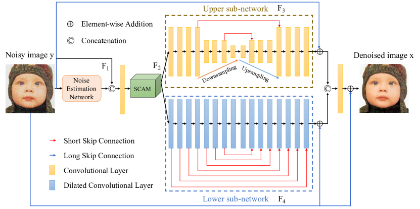
Figure 1: The network structure of the proposed model.

3.1.1 Noise estimation network

To accurately estimate the noise in an image, unlike the noise estimation network of CBDNet Guo2019 and VDN Yue2019 , our noise estimation network contains more convolutional layers, which can make the network extract complex noise information. The architectures of noise estimation sub-networks of the proposed DCANet, CBDNet Guo2019 , AINDNet Kim2020 , and VDN Yue2019 can be seen in Fig. 2. Our estimator has 7 convolutional layers, where the Convolution (Conv), Rectified Linear Units (ReLU) Krizhevsky2012 , Batch Normalization (BN) Ioffe2015 and Tanh Malfliet1996 are used in the network. Specifically, “Conv+ReLU”, “Conv+BN+ReLU” and “Conv+Tanh” are used in the first, the middle, and the last layers respectively. The noise feature $F_{1}$ in Eqn. (2) can be obtained by:

$$F_{0}^{0} =\phi(K_{s}*y),$$ (6)

$$F_{0}^{i+1} =\phi(BN(K_{s}*F_{0}^{i})),i\in\{0,1,2,3,4\},$$

$$F_{1} =\xi(K_{s}*F_{0}^{5}),$$

where $y$, $K_{s}$, and $F_{1}$ are the noisy image, standard convolutional kernel, and the estimated noise level, respectively. $\phi$ and $\xi$ represent the ReLU and Tanh activation functions, respectively. $F_{0}^{0}$ is the feature obtained by the first layer, and $F_{0}^{i+1}$ denotes the features sequentially extracted by the five middle convolutional layers, and $F_{1}$ is the noise feature obtained by the last layer of the noise estimator. The zero padding is used in our noise estimator to keep the feature map size constant.

It should be noted that both our noise estimation network and the estimator in AINDNet Kim2020 have seven convolutional layers. Different from ours, the noise estimation network of the AINDNet has two downsampling operations. Although a larger receptive field size is beneficial to extract more image information, the downsampling operations yet will bring information loss. In particular, compared with the noise estimation sub-networks of the CBDNet, VDN, and AINDNet, our estimation network incorporates multiple BN layers, which not only accelerate network training, but also enhance network performance.

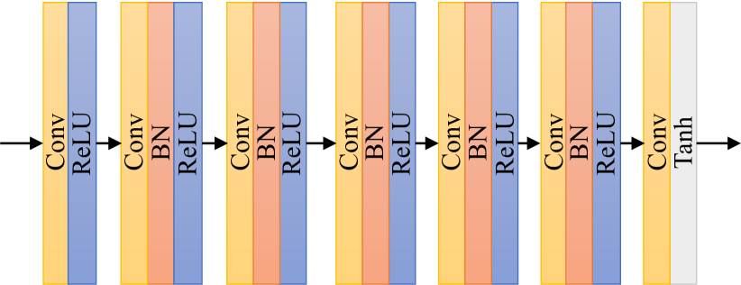
(a) The noise estimation network of our DCANet.

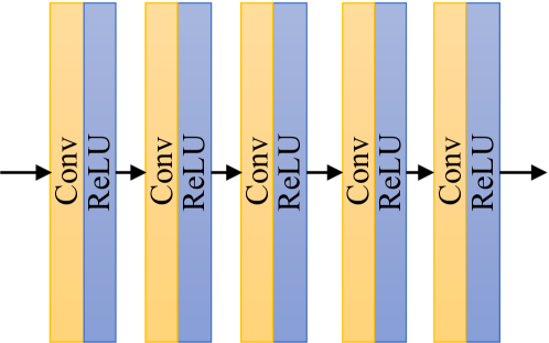
(b) The noise estimation network of CBDNet Guo2019 .

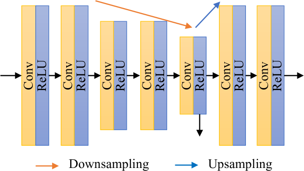
(c) The noise estimation network of AINDNet Kim2020 .

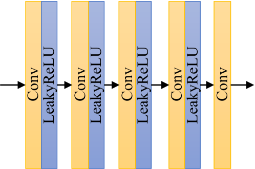
(d) The noise estimation network of VDN Yue2019 .

Figure 2: The noise estimation network architectures of our DCANet (a), CBDNet (b), AINDNet (c), and VDN (d).

3.1.2 Spatial and channel attention module

To leverage the useful features in images, many denoising models employ attention mechanisms to improve their learning ability, such as the ADNet TianX2020 , RDAN Hou2019 , RNAN Zhang2019 , CSANN Wang2021 , and DeamNet Ren2021 . Following the attention network introduced in CSANN Wang2021 , our proposed DCANet also utilizes the spatial and channel attention for feature selection, which is presented in Fig. 3. Our spatial and channel attention module (SCAM) consists of the parallel spatial attention module (SAM) and channel attention module (CAM), which contains the following operations: Conv, PReLU He2015 , Global Average Pooling (GAP) Hu2018 , Global Max Pooling (GMP) Woo2018 , BN, ReLU, Sigmoid Han1995 . The implemental procedure of the SCAM can be expressed as follows:

$$F_{1}^{2} =\varphi(K_{s}*F_{1}^{1}),$$ (7)

$$F_{1}^{3} =K_{s}*F_{1}^{2},$$

$$F_{1}^{4} =\delta(\phi(BN(K_{s}*[GAP(F_{1}^{3}),GMP(F_{1}^{3})])))\cdot F_{1}^{3},$$

$$F_{1}^{5} =\delta(K_{s}*\phi(K_{s}*GAP(F_{1}^{3})))\cdot F_{1}^{3},$$

$$F_{2} =K_{s}*[F_{1}^{4},F_{1}^{5}]+F_{1}^{1},$$

where $F_{1}^{i}$ ($i\in$ {1, 2, 3, 4, 5}) and $F_{2}$ denote the captured features. $\varphi$, $\delta$, and $\phi$ represent PReLU, Sigmod, and ReLU activation functions, respectively. The ’$\cdot$’ and $[,]$ are the element-wise product and concatenation operation. The SCAM is employed to exploit the inter-spatial and inter-channel relationships of the convolutional features. The informative features are retained by the SCAM module, and the unimportant ones are suppressed.

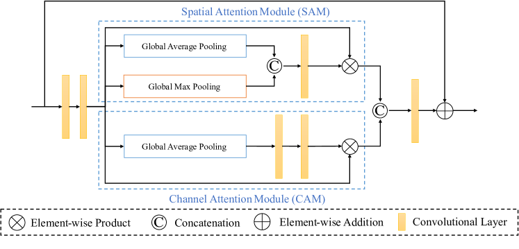
Figure 3: The structure of the SCAM.

3.1.3 Dual convolutional neural network

It has been verified that expanding the width of the denoising network is also a useful way to improve network performance Szegedy2015 . In this work, we develop a dual CNN with two different sub-networks for image denoising, which can be seen in the brown and blue dotted boxes in Fig. 1, where the upper sub-network is a U-shaped network, and the lower branch is a dilated convolution network. It has been verified that using different sub-networks in dual CNN can enhance the performance of the whole network, as the complementary features can be learned by the two different branches Tian2020 ; ZhangT2018 ; Tian2021 . The upper branch of our dual CNN involves the following operations: Conv, ReLU, BN, max-pooling (Downsampling) Ranzato2007 , bilinear interpolation (Upsampling) Huang2020 , and skip connections He2016 ; Huang2017 . The lower branch includes Dilated Convolution (DConv) Yu2015 , ReLU, BN, and the skip connections as well. The outputs of two different branches are concatenated through a concatenation operation.

Compared with the existing dual CNN based denoising models such as the BRDNet Tian2020 and DualCNN Pan2022 , our proposed dual network is designed to own a larger receptive field, which allows the network to capture more contextual information. Specifically, in our dual network, the upper branch employs two times of downsampling to increase the receptive field. However, the downsampling operation may cause the loss of image information. Therefore, two skip connections are applied in the upper sub-networks to suppress the loss. The upsampling operations are employed to recover the size of the feature map.

The lower sub-network applies the dilated convolution to increase the size of the receptive field, and the symmetric skip connections are utilized to speed up network training. Particularly, we adopt the hybrid dilated convolution (HDC) in the lower branch, it has been verified that the HDC can remove the gridding phenomenon effectively and improve network performance Yu2017 ; Wang2018 . The dilated rate of each dilated convolution layer in the lower branch is shown in Table 1.

Table 1: The dilated rates of different layers in the lower sub-network.

Layer	1	2	3	4	5	6	7	8	9	10	11	12	13	14	15	16
Dilated rate	1	2	3	4	5	6	7	8	7	6	5	4	3	2	1	1

3.2 Loss functions

Mean squared error (MSE) is a widely used loss function for optimizing neural networks Yang2019 ; ZhangP2018 . For the AWGN removal, we optimize our DCANet by the following loss function:

$$\mathcal{L} =\frac{1}{2N}\sum_{i=1}^{N}\left\|f(y_{i},\theta)-x_{i}\right\|^{2}$$ (8)

$$=\frac{1}{2N}\sum_{i=1}^{N}\left\|\hat{x}_{i}-x_{i}\right\|^{2},$$

where $x_{i}$, $y_{i}$, and $\hat{x}_{i}$ are the clean, noisy, and denoised images, respectively. $N$ is the number of clean-noisy image patches, and $\theta$ represents the parameters of the DCANet.

For removing the unknown real noise, as the high-frequency textures will be lost due to the square penalty, then the MSE often produces a blurred and overly smoothed visual effect. Therefore, we select the Charbonnier loss Lai2017 as the reconstruction loss to optimize our model for real noise removal. Moreover, to preserve the fidelity and authenticity of the high-frequency details, we utilize the edge loss proposed in Jiang2020 to constrain the loss of the high-frequency components between the ground-truth image $x$ and the denoised image $\hat{x}$.

Our proposed DCANet contains a noise estimator to predict the noise level $\sigma(y)$ in a noisy image $y$. For real noise removal, the estimated noise level should be avoided to be too smooth, especially for the spatially variant noise, which may change dramatically throughout the whole noisy image. Therefore, we employ a total variation (TV) regularizer Guo2019 to restrict the smoothness of the estimated noise level. Therefore, the total loss of our DCANet is expressed as:

$$\mathcal{L}=\mathcal{L}_{char}(\hat{x},x)+\lambda_{edge}\mathcal{L}_{edge}(\hat{x},x)+\lambda_{TV}\mathcal{L}_{TV}(\sigma(y)),$$ (9)

where we empirically set $\lambda_{edge}$ and $\lambda_{TV}$ to 0.1 and 0.05 respectively, and $\mathcal{L}_{char}$ is the Charbonnier loss, which is represented as:

$$\mathcal{L}_{char}=\sqrt{\left\|\hat{x}-x\right\|^{2}+\epsilon^{2}},$$ (10)

where the constant $\epsilon$ is set as $10^{-3}$. $\mathcal{L}_{edge}$ is the edge loss, which can be expressed as:

$$\mathcal{L}_{edge}=\sqrt{\left\|\bigtriangleup{(\hat{x})}-\bigtriangleup{(x)}\right\|^{2}+\epsilon^{2}},$$ (11)

where $\bigtriangleup$ denotes the Laplacian operator Kamgar1999 . $\mathcal{L}_{TV}$ is defined as:

$$\mathcal{L}_{TV}=\left\|\bigtriangledown_{h}{\sigma(y)}\right\|_{2}^{2}+\left\|\bigtriangledown_{v}{\sigma(y)}\right\|_{2}^{2},$$ (12)

where $\bigtriangledown_{h}(\bigtriangledown_{v})$ is the gradient operator along the horizontal (vertical) direction.

4 Experiments and results

4.1 Datasets

The DIV2K dataset Agustsson2017 containing 800 high-resolution color images was used to train the proposed DCANet for the AWGN removal, and we resized these high-resolution images into the images of the size $512\times 512$. Moreover, the images were grayscaled to train the DCANet for grayscale image denoising. According to the size of the receptive field of the DCANet, the training images were randomly cropped into patches of the size $140\times 140$. The AWGN within a noise level range of $[0,75]$ is added to the clean image patches to generate their noisy counterparts. To augment the training samples, rotation and flipping were utilized. We tested our model on five public commonly used datasets, including Set12 Roth2005 , BSD68 Roth2005 , CBSD68 Roth2005 , Kodak24 Kodak24 and McMaster Zhang2011 .

For real noise removal, we select the SIDD training data Abdelhamed2018 and RENOIR dataset Anaya2018 for model training. The SIDD training data and the RENOIR dataset consist of 320 and 240 pairs of noisy images and the near noise-free counterparts, respectively. We randomly cut the images in these datasets into image patches of size $140\times 140$, and applied rotation and flipping operations for data augmentation. The SIDD validation set Abdelhamed2018 and DND sRGB dataset Plotz2017 were used for model evaluation.

4.2 Experimental settings

All our experiments were performed on a PC equipped with a CPU of Intel(R) Core(TM) i7-11700KF, 32 GB RAM, and a GPU of NVIDIA GeForce RTX 3080Ti. The proposed DCANet was trained for grayscale and color images, respectively. The training of the DCANet for the synthetic noise cost about 48 hours. For real image denoising, it took about 45 hours to train the model.

The network parameters of the DCANet were optimized by the Adam optimizer Kingma2014 . For the AWGN removal, the DCANet was trained for 600,000 iterations, during which the initial learning rate is $10^{-4}$ and then decreases by half every 100,000 iterations, and the batch size was set to 24. For real image denoising, we used 120 epochs to train the model, during which the initial learning rate was $2\times 10^{-4}$ and steadily reduced to $10^{-6}$ using cosine annealing strategy Loshchilov2017 , the batch size was set to 16. For other hyper-parameters of the Adam algorithm, we used the default settings.

4.3 Ablation study

To verify the effectiveness of the proposed denoising architecture, especially the effect of SCAM, dual CNN, and skip connections, we trained ten different networks for grayscale image denoising. The ten different models and their corresponding performance are shown in Table 2. The Set12 Roth2005 dataset was utilized for our ablation evaluation, and the noise level was set to 75.

In Table 2, one can find that short and long skip connections can improve the network performance. Besides, the denoising performance of the models using only a single attention mechanism (SAM or CAM) is better than that of the model using serial attention mechanisms, but lower than that of the model using parallel attention mechanisms (SCAM in the proposed model), which shows the effectiveness of the proposed SCAM. In addition, the denoising performance of the model using a single sub-network is inferior to the dual CNN structure. The results validate that using SCAM, dual CNN, and skip connections can improve the model performance.

Table 2: Quantitative comparison results of the ten models containing different components on the Set12 dataset. The noise level is set to 75. The best results are bolded.

Model ID	Models	PSNR	SSIM
1	DCANet without short skip connection	25.60	0.7356
2	DCANet without long skip connection	25.72	0.7447
3	DCANet without SCAM	25.65	0.7406
4	DCANet without SAM	25.73	0.7453
5	DCANet without CAM	25.71	0.7444
6	DCANet with serial attention mechanism ( SAM(front) and CAM (behind) )	25.62	0.7377
7	DCANet with serial attention mechanism ( CAM(front) and SAM (behind) )	25.66	0.7409
8	DCANet with only upper sub-network	25.52	0.7325
9	DCANet with only lower sub-network	25.70	0.7443
10	Proposed DCANet model	$\mathbf{25.75}$	$\mathbf{0.7458}$

4.4 The additive white Gaussian noise removal

In this subsection, we show the results of our DCANet on grayscale and color images corrupted by the AWGN. The BM3D Dabov2007 , WNNM Gu2014 , MCWNNM Xu2017 , TNRD Chen2017 , DnCNN Zhang2017 , BUIFD Helou2020 , IRCNN ZhangZGZ2017 , FFDNet Zhang2018 , BRDNet Tian2020 , ADNet TianX2020 , DudeNet Tian2021 , DSNetB Peng2019 , RIDNet Anwar2019 , AINDNet Kim2020 and AirNet Li2022 were used to compare with our DCANet.

Table 3 lists the PSNR values at different noise levels of the compared denoising models on the Set12 dataset. One can see that the denoising performances of the DCANet are slightly behind the BRDNet and ADNet at noise levels 15 and 25, however our DACNet beats other methods at noise level 50. It also should be noted that for the image “Barbara", the traditional methods BM3D and WNNM obtain significant denoising results, we think the reason is that this image contains rich repetitive structures, and the non-local self-similarity learning based methods can capture such structures better.

Table 3: Quantitative comparison results on the Set12 dataset. The three best results are respectively emphasized in red, blue and green.

Noise levels	Models	C.man	House	Peppers	Starfish	Monar.	Airpl.	Parrot	Lena	Barbara	Boat	Man	Couple	Average
$\sigma$=15	BM3D Dabov2007	31.91	34.93	32.69	31.14	31.85	31.07	31.37	34.26	33.10	32.13	31.92	31.10	32.37
	WNNM Gu2014	32.17	35.13	32.99	31.82	32.71	31.39	31.62	34.27	33.60	32.27	32.11	32.17	32.70
	TNRD Chen2017	32.19	34.53	33.04	31.75	32.56	31.46	31.63	34.24	32.13	32.14	32.23	32.11	32.50
	DnCNN-S Zhang2017	32.61	34.97	33.30	32.20	33.09	31.70	31.83	34.62	32.64	32.42	32.46	32.47	32.86
	IRCNN ZhangZGZ2017	32.55	34.89	33.31	32.02	32.82	31.70	31.84	34.53	32.43	32.34	32.40	32.40	32.77
	BUIFD Helou2020	31.74	34.78	32.80	31.92	32.77	31.34	31.39	34.38	31.68	32.18	32.25	32.22	32.46
	FFDNet Zhang2018	32.43	35.07	33.25	31.99	32.66	31.57	31.81	34.62	32.54	32.38	32.41	32.46	32.77
	BRDNet Tian2020	32.80	35.27	33.47	32.24	33.35	31.85	32.00	34.75	32.93	32.55	32.50	32.62	33.03
	ADNet TianX2020	32.81	35.22	33.49	32.17	33.17	31.86	31.96	34.71	32.80	32.57	32.47	32.58	32.98
	DudeNet Tian2021	32.71	35.13	33.38	32.29	33.28	31.78	31.93	34.66	32.73	32.46	32.46	32.49	32.94
	DCANet	32.43	35.13	33.09	32.06	33.16	31.55	31.80	34.70	32.76	32.42	32.40	32.48	32.83
$\sigma$=25	BM3D Dabov2007	29.45	32.85	30.16	28.56	29.25	28.42	28.93	32.07	30.71	29.90	29.61	29.71	29.97
	WNNM Gu2014	29.64	33.22	30.42	29.03	29.84	28.69	29.15	32.24	31.24	30.03	29.76	29.82	30.26
	TNRD Chen2017	29.72	32.53	30.57	29.02	29.85	28.88	29.18	32.00	29.41	29.91	29.87	29.71	30.06
	DnCNN-S Zhang2017	30.18	33.06	30.87	29.41	30.28	29.13	29.43	32.44	30.00	30.21	30.10	30.12	30.43
	IRCNN ZhangZGZ2017	30.08	33.06	30.88	29.27	30.09	29.12	29.47	32.43	29.92	30.17	30.04	30.08	30.38
	BUIFD Helou2020	29.42	33.03	30.48	29.21	30.20	28.99	28.94	32.20	29.18	29.97	29.88	29.90	30.12
	FFDNet Zhang2018	30.10	33.28	30.93	29.32	30.08	29.04	29.44	32.57	30.01	30.25	30.11	30.20	30.44
	BRDNet Tian2020	31.39	33.41	31.04	29.46	30.50	29.20	29.55	32.65	30.34	30.33	30.14	30.28	30.61
	ADNet TianX2020	30.34	33.41	31.14	29.41	30.39	29.17	29.49	32.61	30.25	30.37	30.08	30.24	30.58
	DudeNet Tian2021	30.23	33.24	30.98	29.53	30.44	29.14	29.48	32.52	30.15	30.24	30.08	30.15	30.52
	DCANet	30.18	33.39	30.84	29.42	30.51	29.10	29.49	32.72	30.49	30.35	30.14	30.26	30.57
$\sigma$=50	BM3D Dabov2007	26.13	29.69	26.68	25.04	25.82	25.10	25.90	29.05	27.22	26.78	26.81	26.46	26.72
	WNNM Gu2014	26.45	30.33	26.95	25.44	26.32	25.42	26.14	29.25	27.79	26.97	26.94	26.64	27.05
	TNRD Chen2017	26.62	29.48	27.10	25.42	26.31	25.59	26.16	28.93	25.70	26.94	26.98	26.50	26.81
	DnCNN-S Zhang2017	27.03	30.00	27.32	25.70	26.78	25.87	26.48	29.39	26.22	27.20	27.24	26.90	27.18
	IRCNN ZhangZGZ2017	26.88	29.96	27.33	25.57	26.61	25.89	26.55	29.40	26.24	27.17	27.17	26.88	27.14
	BUIFD Helou2020	25.44	29.76	26.50	24.87	26.49	25.34	25.07	28.81	25.49	26.59	26.87	26.34	26.46
	FFDNet Zhang2018	27.05	30.37	27.54	25.75	26.81	25.89	26.57	29.66	26.45	27.33	27.29	27.08	27.32
	BRDNet Tian2020	27.44	30.53	27.67	25.77	26.97	25.93	26.66	25.93	26.66	27.38	27.27	27.17	27.45
	ADNet TianX2020	27.31	30.59	27.69	25.70	26.90	25.88	26.56	29.59	26.64	27.35	27.17	27.07	27.37
	DudeNet Tian2021	27.22	30.27	27.51	25.88	26.93	25.88	26.50	29.45	26.49	27.26	27.19	26.97	27.30
	DCANet	27.41	30.64	27.57	25.89	27.08	25.97	26.67	29.87	27.33	27.47	27.33	27.25	27.54

Table 4 presents the average SSIM results of the compared models on the Set12 dataset. As can be seen from the table, our DCANet also produces competitive results.

Table 4: Quantitative comparison results on the Set12 dataset. The three best results are respectively emphasized in red, blue and green.

Models	$\sigma$=15	$\sigma$=25	$\sigma$=50
BM3D Dabov2007	0.896	0.851	0.766
WNNM Gu2014	0.894	0.846	0.756
TNRD Chen2017	0.896	0.851	0.768
DnCNN-S Zhang2017	0.903	0.862	0.783
IRCNN ZhangZGZ2017	0.901	0.860	0.780
BUIFD Helou2020	0.899	0.855	0.755
FFDNet Zhang2018	0.903	0.864	0.791
BRDNet Tian2020	0.906	0.866	0.794
ADNet TianX2020	0.905	0.865	0.791
RIDNet Anwar2019	0.906	0.867	0.793
DCANet	0.903	0.866	0.798

Table 5 reports the quantitative results on the BSD68 dataset of the compared denoising models. It can be found that the RIDNet obtains leading performance at noise levels 15 and 25. Our proposed model can obtain competitive denoising results at all tested noise levels, and especially our model outperforms other denoising methods at noise level 50.

Table 5: Quantitative comparison results on the BSD68 dataset. The three best results are respectively emphasized in red, blue and green.

Metrics	Models	$\sigma$=15	$\sigma$=25	$\sigma$=50
PSNR	BM3D Dabov2007	31.07	28.57	25.62
	WNNM Gu2014	31.37	28.83	25.87
	DnCNN-S Zhang2017	31.72	29.23	26.23
	TNRD Chen2017	31.42	28.92	25.97
	IRCNN ZhangZGZ2017	31.63	29.15	26.19
	BUIFD Helou2020	31.35	28.75	25.11
	FFDNet Zhang2018	31.63	29.19	26.29
	DSNetB Peng2019	31.69	29.22	26.29
	RIDNet Anwar2019	31.81	29.34	26.40
	BRDNet Tian2020	31.79	29.29	26.36
	ADNet TianX2020	31.74	29.25	26.29
	AINDNet Kim2020	31.69	29.26	26.32
	DudeNet Tian2021	31.78	29.29	26.31
	DCANet	31.71	29.31	26.44
SSIM	BM3D Dabov2007	0.872	0.802	0.687
	WNNM Gu2014	0.878	0.810	0.698
	TNRD Chen2017	0.883	0.816	0.703
	DnCNN-S Zhang2017	0.891	0.828	0.719
	IRCNN ZhangZGZ2017	0.888	0.825	0.717
	BUIFD Helou2020	0.886	0.819	0.682
	FFDNet Zhang2018	0.890	0.830	0.726
	BRDNet Tian2020	0.893	0.831	0.727
	ADNet TianX2020	0.892	0.829	0.722
	RIDNet Anwar2019	0.893	0.833	0.727
	DCANet	0.891	0.831	0.730

Fig. 4 shows the visual comparison results on the “test003” image at noise level 50 of different denoising models. One can find that compared with other models, the DCANet obtains better denoising performance, both quantitatively and qualitatively.

It can be seen from our experimental results on the grayscale images that our DCANet can achieve competitive denoising performance compared with other state-of-the-art methods. Especially, a trend can be discovered from Table 3, Table 4, and Table 5, that for grayscale image denoising, our model becomes more effective as the noise power increases.

(a) (I)

(b) (II)

(c) (III)

(d) (IV)

(e) (V)

(f) (VI)

(g) (VII)

(h) (VIII)

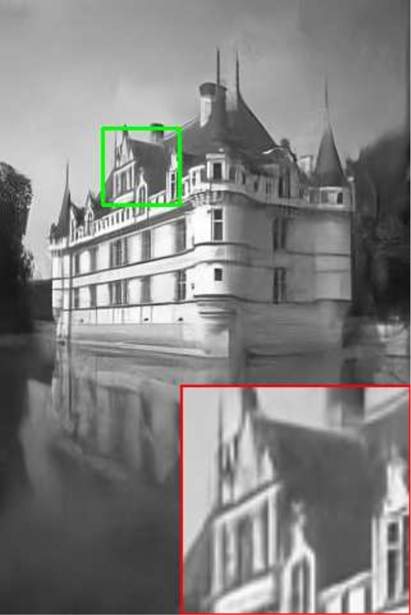
(i) (IX)

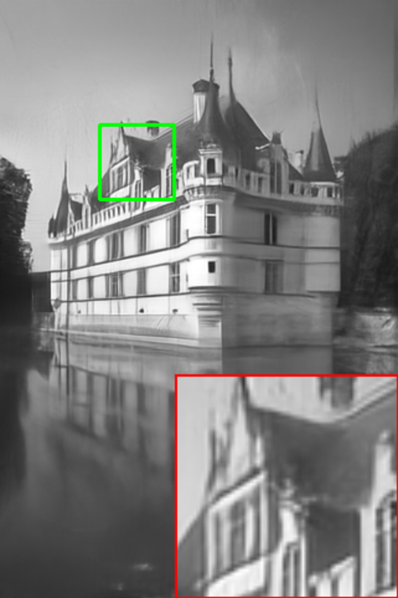
(j) (X)

Figure 4: Visual comparison results on the “test003” image from the BSD68 dataset at the noise level 50. (I) Ground-truth image, (II) Noisy image / 14.15dB, (III) BM3D / 26.21dB, (IV) WNNM / 26.50dB, (V) DnCNN-S / 26.90dB, (VI) IRCNN / 26.85dB, (VII) BUIFD / 26.32dB, (VIII) FFDNet / 26.92dB, (IX) ADNet / 27.06dB, (X) DCANet / 27.18dB.

For the noise removal evaluation on color images, the CBSD68, Kodak24, and McMaster datasets were applied. Table 6 lists the average PSNR values at different noise levels of many models on three datasets. It can be seen that our model obtains leading denoising results compared to other state-of-the-art denoising models.

Table 6: Quantitative comparison results on three commonly used color datasets. The three best results are respectively emphasized in red, blue and green.

Datasets	Models	$\sigma$=15	$\sigma$=25	$\sigma$=35	$\sigma$=50	$\sigma$=75
CBSD68	CBM3D Dabov2007	33.52	30.71	28.89	27.38	25.74
	MCWNNM Xu2017	30.91	27.61	25.88	23.18	21.21
	CDnCNN-S Zhang2017	33.89	31.23	29.58	27.92	24.47
	IRCNN ZhangZGZ2017	33.86	31.16	29.50	27.86	-
	BUIFD Helou2020	33.65	30.76	28.82	26.61	23.64
	FFDNet Zhang2018	33.87	31.21	29.58	27.96	26.24
	DSNetB Peng2019	33.91	31.28	-	28.05	-
	RIDNet Anwar2019	34.01	31.37	-	28.14	-
	BRDNet Tian2020	34.10	31.43	29.77	28.16	26.43
	ADNet TianX2020	33.99	31.31	29.66	28.04	26.33
	DudeNet Tian2021	34.01	31.34	29.71	28.09	26.40
	AirNet Li2022	33.92	31.26	-	28.01	-
	DCANet	34.05	31.45	29.86	28.28	26.61
Kodak24	CBM3D Dabov2007	34.28	31.68	29.90	28.46	26.82
	MCWNNM Xu2017	32.00	28.76	27.02	21.18	18.06
	CDnCNN-S Zhang2017	34.48	32.03	30.46	28.85	25.04
	IRCNN ZhangZGZ2017	34.56	32.03	30.43	28.81	-
	BUIFD Helou2020	34.41	31.77	29.94	27.74	24.67
	FFDNet Zhang2018	34.63	32.13	30.57	28.98	27.27
	DSNetB Peng2019	34.63	32.16	-	29.05	-
	BRDNet Tian2020	34.88	32.41	30.80	29.22	27.49
	ADNet TianX2020	34.76	32.26	30.68	29.10	27.40
	DudeNet Tian2021	34.81	32.26	30.69	29.10	27.39
	AirNet Li2022	34.68	32.21	-	29.06	-
	DCANet	34.85	32.43	30.91	29.36	27.69
McMaster	CBM3D Dabov2007	34.06	31.66	29.92	28.51	26.79
	MCWNNM Xu2017	32.75	29.39	27.44	21.37	18.16
	CDnCNN-S Zhang2017	33.44	31.51	30.14	28.61	25.10
	IRCNN ZhangZGZ2017	34.58	32.18	30.59	28.91	-
	BUIFD Helou2020	33.84	31.06	28.87	26.20	22.75
	FFDNet Zhang2018	34.66	32.35	30.81	29.18	27.33
	DSNetB Peng2019	34.67	32.40	-	29.28	-
	BRDNet Tian2020	35.08	32.75	31.15	29.52	27.72
	ADNet TianX2020	34.93	32.56	31.00	29.36	27.53
	AirNet Li2022	34.70	32.44	-	29.26	-
	DCANet	34.84	32.62	31.16	29.59	27.81

Table 7 reports the average SSIM values at multiple noise levels of the compared denoising methods on three color image datasets. One can find that the DCANet also generates better results.

Table 7: Quantitative comparison results on three commonly used color datasets. The three best results are respectively emphasized in red, blue and green.

Datasets	Models	$\sigma$=15	$\sigma$=25	$\sigma$=50
CBSD68	CDnCNN-B Zhang2017	0.929	0.883	0.790
	IRCNN ZhangZGZ2017	0.929	0.882	0.790
	BUIFD Helou2020	0.930	0.882	0.777
	FFDNet Zhang2018	0.929	0.882	0.789
	ADNet TianX2020	0.933	0.889	0.797
	AirNet Li2022	0.933	0.888	0.798
	DCANet	0.932	0.888	0.804
Kodak24	CDnCNN-B Zhang2017	0.920	0.876	0.791
	IRCNN ZhangZGZ2017	0.920	0.877	0.793
	BUIFD Helou2020	0.923	0.879	0.786
	FFDNet Zhang2018	0.922	0.878	0.794
	ADNet TianX2020	0.924	0.882	0.798
	AirNet Li2022	0.924	0.882	0.799
	DCANet	0.925	0.885	0.811
McMaster	CDnCNN-B Zhang2017	0.904	0.869	0.799
	IRCNN ZhangZGZ2017	0.920	0.882	0.807
	BUIFD Helou2020	0.901	0.847	0.733
	FFDNet Zhang2018	0.922	0.886	0.815
	ADNet TianX2020	0.927	0.894	0.825
	AirNet Li2022	0.925	0.891	0.822
	DCANet	0.924	0.893	0.831

Fig. 5 presents the visual comparison results on the “kodim23” image from the Kodak24 dataset of different denoising models. One can see that our model obtains a visual appealing result, and a favorable trade-off between image detail preservation and noise reduction is obtained.

(a) (I)

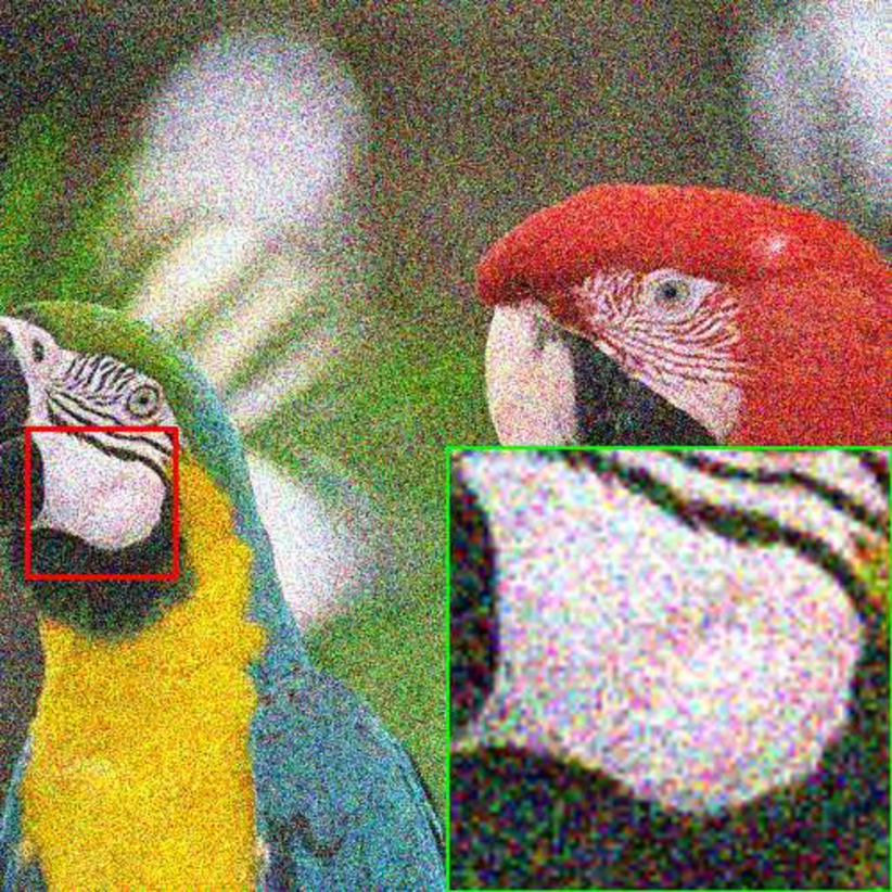
(b) (II)

(c) (III)

(d) (IV)

(e) (V)

(f) (VI)

(g) (VII)

(h) (VIII)

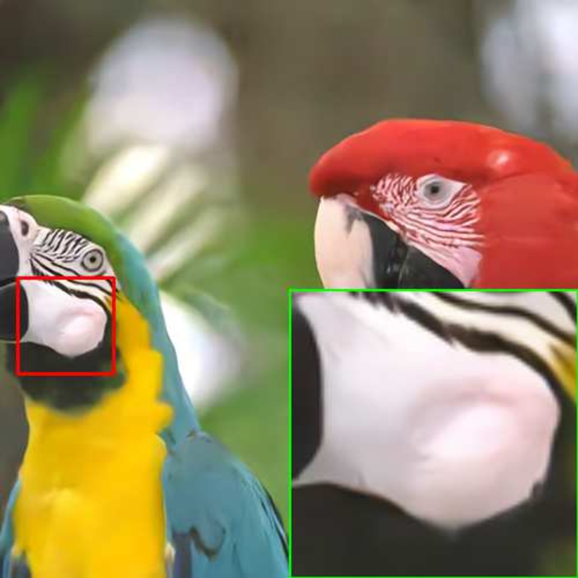
(i) (IX)

(j) (X)

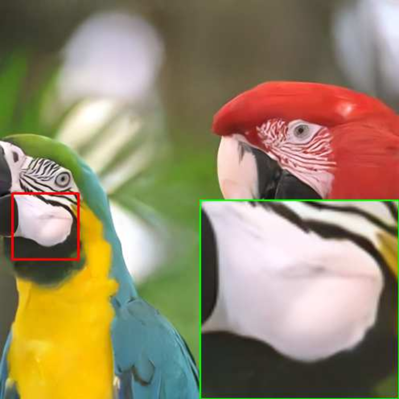
(k) (XI)

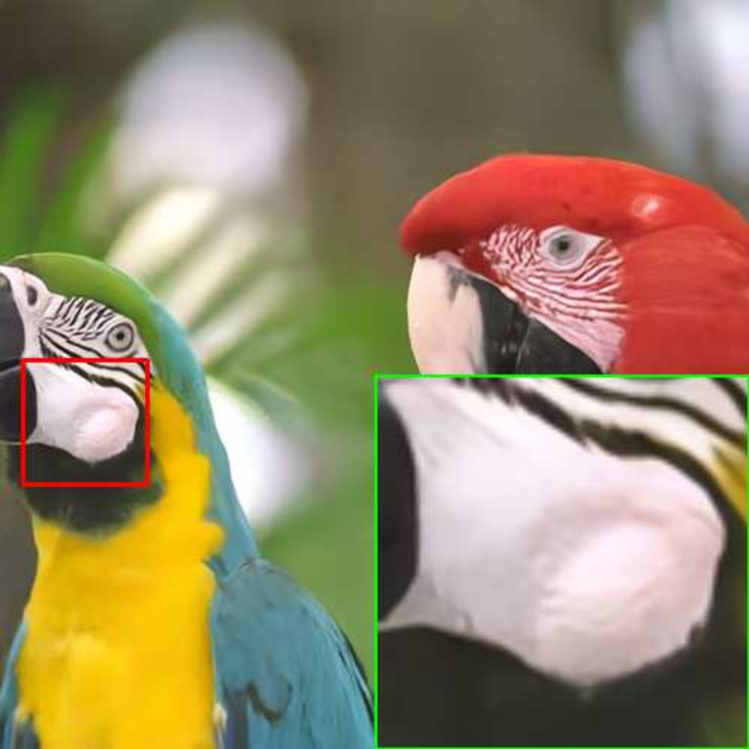
(l) (XII)

Figure 5: Visual comparison results on the “kodim23” image from the Kodak24 dataset at the noise level 50. (I) Ground-truth image, (II) Noisy image / 14.16dB, (III) CBM3D / 30.95dB, (IV) MCWNNM / 25.25dB, (V) CDnCNN-S / 31.47dB, (VI) CDnCNN-B / 31.12dB, (VII) IRCNN / 31.16dB, (VIII) BUIFD / 29.41dB, (IX) FFDNet / 31.50dB, (X) ADNet / 31.47dB, (XI) AirNet / 31.50dB, (XII) DCANet / 31.86dB.

4.5 Real noise removal

For real noise removal, we evaluated the denoising methods on two commonly used public datasets: the SIDD validation set and the DND sRGB images. The two datasets contain real noisy images and near noise-free counterparts, and the counterparts can be provided as the ground truth, which can be utilized to obtain the PSNR and SSIM values.

Table 8 lists the average PSNR and SSIM values of the compared models on the SIDD validation set and the DND sRGB images. One can see that the DCANet model obtains effective denoising performance.

Table 8: Quantitative comparison results on the SIDD validation set and the DND sRGB images. The three best results are respectively emphasized in red, blue and green.

Dataset	Metrics	MCWNNM Xu2017	TWSC Xu2018	DnCNN-B Zhang2017	CBDNet Guo2019	RIDNet Anwar2019	AINDNet Kim2020	VDN Yue2019	DCANet
SIDD	PSNR	33.40	35.33	23.66	30.78	38.71	38.95	39.28	39.27
	SSIM	0.879	0.933	0.583	0.951	0.954	0.952	0.956	0.956
DND	PSNR	37.38	37.94	37.90	38.06	39.23	39.37	39.38	39.57
	SSIM	0.929	0.940	0.943	0.942	0.953	0.951	0.952	0.953

Fig. 6 shows the visual results of the compared models for real noise removal. It can be found the MCWNNM, TWSC, and CDnCNN-B generated unsatisfactory visual effects. In contrast, the AINDNet, VDN, and the proposed DCANet achieved much better visual quality and PSNR/SSIM values.

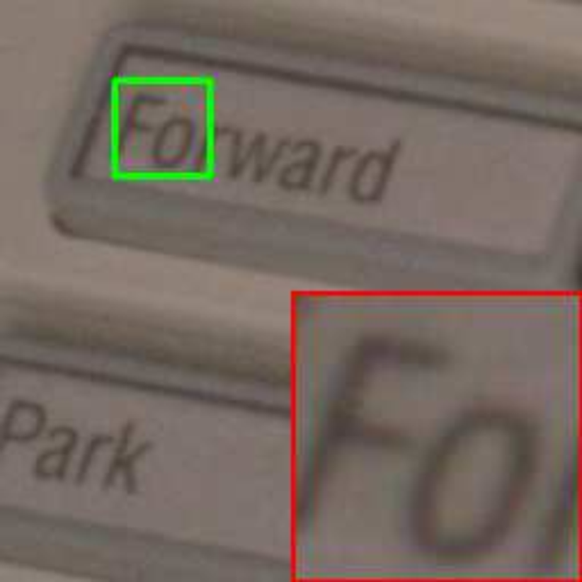
(a) (I)

(b) (II)

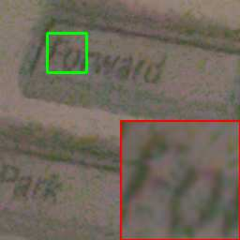
(c) (III)

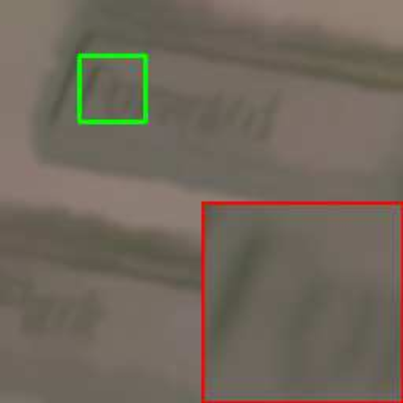
(d) (IV)

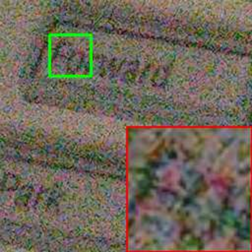
(e) (V)

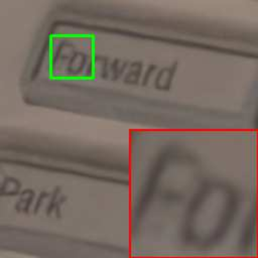
(f) (VI)

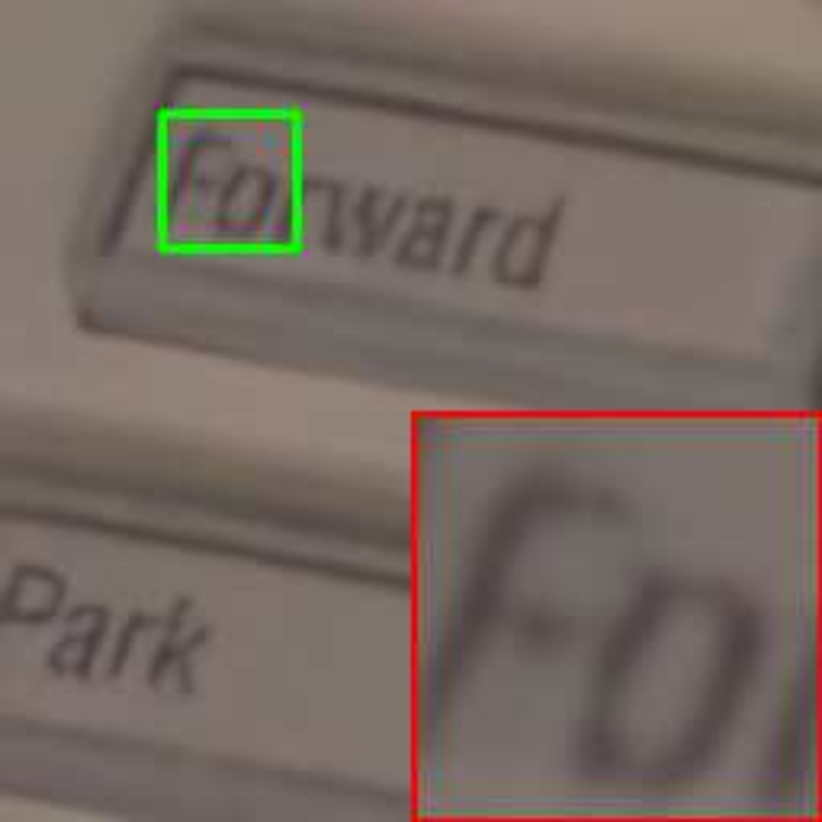
(g) (VII)

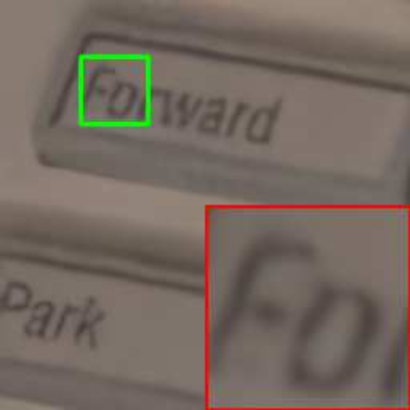
(h) (VIII)

Figure 6: Visual comparison results on the “11_4” image from the SIDD validation set. (I) Ground-truth image / (PSNR/SSIM), (II) Noisy image / (18.25/0.169), (III) MCWNNM / (28.63/0.725), (IV) TWSC / (30.42/0.837), (V) CDnCNN-B / (20.76/0.231), (VI) AINDNet / (36.24/0.904), (VII) VDN / (36.39/0.907), (VIII) DCANet / (36.36/0.912).

4.6 Model complexity analysis

We evaluated the network complexity of the proposed DCANet from the perspectives of the running time, the floating point operations per second (FLOPs), and the number of network parameters. The codes of all the compared denoising models are from the original authors. The BM3D Dabov2007 , WNNM Gu2014 and MCWNNM Xu2017 were run in Matlab (R2020a) environment. The DnCNN-B Zhang2017 , BUIFD Helou2020 , IRCNN ZhangZGZ2017 , FFDNet Zhang2018 , BRDNet Tian2020 , CBDNet Guo2019 , RIDNet Anwar2019 , DudeNet Tian2021 , AINDNet Kim2020 , VDN Yue2019 , ADNet TianX2020 , AirNet Li2022 , and the proposed DCANet were implemented in PyCharm (2021) environment.

Three randomly chosen grayscale and color noisy images of different sizes were used to evaluate the runtime of different denoising models. The noise level was set to 25. We obtained the runtime of every tested method on each image by averaging the time of 20 implementations. It should be noted that our experiments neglected the memory transfer time between the CPU and GPU. Table 9 lists the runtime of the tested denoising methods. It can be found that our DCANet has a fast speed for both grayscale and color images.

Table 9: Runtime (in seconds) comparison of different denoising models on different images.

Devices	Models	$256\times 256$		$512\times 512$		$1024\times 1024$
		Gray	Color	Gray	Color	Gray	Color
CPU	BM3D Dabov2007	0.458	0.593	2.354	3.771	9.782	12.818
	WNNM Gu2014	63.867	-	277.003	-	1150.842	-
	MCWNNM Xu2017	-	62.777	-	277.623	-	1120.112
GPU	DnCNN-B Zhang2017	0.032	0.032	0.037	0.037	0.057	0.057
	IRCNN ZhangZGZ2017	0.030	0.030	0.030	0.030	0.030	0.030
	BUIFD Helou2020	0.035	0.037	0.050	0.053	0.112	0.123
	FFDNet Zhang2018	0.031	0.030	0.031	0.030	0.032	0.030
	AINDNet Kim2020	-	0.531	-	2.329	-	9.573
	VDN Yue2019	0.144	0.162	0.607	0.597	2.367	2.376
	ADNet TianX2020	0.031	0.033	0.035	0.045	0.051	0.093
	AirNet Li2022	-	0.143	-	0.498	-	2.501
	DCANet	0.058	0.059	0.099	0.104	0.252	0.258

Table 10 reports the number of parameters and FLOPs of different models on grayscale and color images, respectively. It can be observed from Table 10 that some state-of-the-art image blind denoising methods have large numbers of parameters, these models are usually equipped with complex model structures, however the proposed DCANet can obtain competitive or even better performance. For those models have the similar number of parameters, like the BUIFD, BRDNet, DudeNet, and RIDNet, our model achieve better results in most of the tested denoising tasks, especially in color image denoising and real noise removal. Namely, our model obtains a favorable tradeoff between network complexity and denoising performance.

Table 10: The number of parameters (in K) and FLOPs (in G) of different models.

Models	Model Parameters		FLOPs
	Gray	Color	$256\times 256\times 1$	$256\times 256\times 3$
DnCNN-B Zhang2017	666	668	21.93	22.12
IRCNN ZhangZGZ2017	186	188	6.08	6.15
BUIFD Helou2020	1186	1196	35.31	35.65
FFDNet Zhang2018	485	852	3.97	3.14
BRDNet Tian2020	1113	1117	36.48	36.63
CBDNet Guo2019	-	4365	-	20.14
RIDNet Anwar2019	1497	1499	48.90	48.98
VDN Yue2019	7810	7817	24.47	24.70
ADNet TianX2020	519	521	17.08	17.15
AINDNet Kim2020	-	13764	-	-
DudeNet Tian2021	1077	1079	35.35	35.43
AirNet Li2022	-	8930	-	150.64
DCANet	1382	1389	37.65	37.88

5 Conclusion

In this paper, we propose a dual convolutional neural network with attention (DCANet) for image blind denoising. The proposed DCANet is composed of a noise estimation network, an attention module, and a dual convolutional denoising network. The noise estimation network is applied to estimate the noise in a noisy image. The attention module consists of spatial and channel attention block, and is utilized to filter unimportant information. The dual convolutional denoising network contains two different branches, which not only widens the network to improve its learning ability, but also can capture the complementary image features to enhance the denoising effect. To the best of our knowledge, the combination of the dual CNN and the attention mechanism for image blind denoising has not been investigated before.

Compared with the state-of-the-art denoising models, the proposed DCANet obtains competitive denoising performance. Our proposed DCANet also obtains a favorable trade-off between model complexity and denoising ability, therefore the model can be an option for the practical image denoising tasks. In the future, we will further investigate the noise estimation network to obtain more accurate noise estimation. The application of the DCANet on other low-level visual tasks such as image deraining and super-resolution will also be addressed.

Declarations

Funding The Natural Science Foundation of China No. 61863037, No. 41971392, and the Applied Basic Research Foundation of Yunnan Province under grant No. 202001AT070077.

Authors contribution statement Wencong Wu conceived and designed the study. Wencong Wu, Guannan Lv, and Yingying Duan performed the experiments. Wencong Wu, and Peng Liang were responsible for drawing figures and tables. Data analysis and collation were carried out by Guannan Lv, and Yingying Duan. Wencong Wu, Yungang Zhang, and Yuelong Xia wrote the paper. Yungang Zhang provided the funding support. Wencong Wu, Yungang Zhang, and Yuelong Xia reviewed and edited the manuscript. All authors read and approved the manuscript.

Ethical and informed consent for data used The datasets used for this work comply with ethical standards, and the authors were given permission to access these datasets.

Data availability and access If necessary, data involved in this work can be provided by the corresponding author, and the code of this work is accessible on https://github.com/WenCongWu/DCANet.

Competing Interests The authors declare that they have no conflicts of interest to this work. The authors declare that they do not have any commercial or associative interest that represents a conflict of interest in connection with the work submitted.

References

- \bibcommenthead
- (1) Buades, A., Coll, B. & Morel, J. A non-local algorithm for image denoising. IEEE Conference on Computer Vision and Pattern Recognition 60–65 (2005) .
- (2) Dabov, K., Foi, A., Katkovnik, V. & Egiazarian, K. O. Image denoising by sparse 3-d transform-domain collaborative filtering. IEEE Trans. Image Process. 16 (8), 2080–2095 (2007) .
- (3) Xu, J., Zhang, L. & Zhang, D. A trilateral weighted sparse coding scheme for real-world image denoising. European Conference on Computer Vision 11212, 21–38 (2018) .
- (4) Gu, S., Zhang, L., Zuo, W. & Feng, X. Weighted nuclear norm minimization with application to image denoising. IEEE Conference on Computer Vision and Pattern Recognition 2862–2869 (2014) .
- (5) Xu, J., Zhang, L., Zhang, D. & Feng, X. Multi-channel weighted nuclear norm minimization for real color image denoising. IEEE International Conference on Computer Vision 1105–1113 (2017) .
- (6) Zhang, K., Zuo, W., Chen, Y., Meng, D. & Zhang, L. Beyond a gaussian denoiser: Residual learning of deep CNN for image denoising. IEEE Trans. Image Process. 26 (7), 3142–3155 (2017) .
- (7) Chatterjee, P. & Milanfar, P. Is denoising dead? IEEE Transactions on Image Processing 19 (4), 895–911 (2010) .
- (8) Zhang, K., Zuo, W. & Zhang, L. Ffdnet: Toward a fast and flexible solution for cnn-based image denoising. IEEE Trans. Image Process. 27 (9), 4608–4622 (2018) .
- (9) Guo, S., Yan, Z., Zhang, K., Zuo, W. & Zhang, L. Toward convolutional blind denoising of real photographs. IEEE Conference on Computer Vision and Pattern Recognition 1712–1722 (2019) .
- (10) Helou, M. E. & Süsstrunk, S. Blind universal bayesian image denoising with gaussian noise level learning. IEEE Trans. Image Process. 29, 4885–4897 (2020) .
- (11) Li, B. et al. All-in-one image restoration for unknown corruption. IEEE Conference on Computer Vision and Pattern Recognition 17431–17441 (2022) .
- (12) Xue, T. & Ma, P. Tc-net: transformer combined with cnn for image denoising. Applied Intelligence 53 (6), 6753–6762 (2023) .
- (13) Xiaohua, Z., Qiusheng, L. & Dan, Z. Total generalized variational-liked network for image denoising. Applied Intelligence 1–18 (2022) .
- (14) Tian, C., Xu, Y. & Zuo, W. Image denoising using deep CNN with batch renormalization. Neural Networks 121, 461–473 (2020) .
- (15) Jinshan, P. et al. Learning dual convolutional neural networks for low-level vision. IEEE Conference on Computer Vision and Pattern Recognition 3070–3079 (2018) .
- (16) Anwar, S. & Barnes, N. Real image denoising with feature attention. International Conference on Computer Vision 3155–3164 (2019) .
- (17) Tian, C. et al. Attention-guided CNN for image denoising. Neural Networks 124, 117–129 (2020) .
- (18) Zhang, K., Zuo, W., Gu, S. & Zhang, L. Learning deep CNN denoiser prior for image restoration. IEEE Conference on Computer Vision and Pattern Recognition 2808–2817 (2017) .
- (19) Peng, Y. et al. Dilated residual networks with symmetric skip connection for image denoising. Neurocomputing 345, 67–76 (2019) .
- (20) Soh, J. W. & Cho, N. I. Deep universal blind image denoising. International Conference on Pattern Recognition 747–754 (2020) .
- (21) Yue, Z., Yong, H., Zhao, Q., Meng, D. & Zhang, L. Variational denoising network: Toward blind noise modeling and removal. Advances in Neural Information Processing Systems 1688–1699 (2019) .
- (22) Kim, Y., Soh, J. W., Park, G. Y. & Cho, N. I. Transfer learning from synthetic to real-noise denoising with adaptive instance normalization. IEEE Conference on Computer Vision and Pattern Recognition 3479–3489 (2020) .
- (23) Du, B., Wei, Q. & Liu, R. An improved quantum-behaved particle swarm optimization for endmember extraction. IEEE Trans. Geosci. Remote. Sens. 57 (8), 6003–6017 (2019) .
- (24) Li, J., Lu, G., Zhang, B., You, J. & Zhang, D. Shared linear encoder-based multikernel gaussian process latent variable model for visual classification. IEEE Trans. Cybern. 51 (2), 534–547 (2021) .
- (25) Liang, X., Zhang, D., Lu, G., Guo, Z. & Luo, N. A novel multicamera system for high-speed touchless palm recognition. IEEE Trans. Syst. Man Cybern. Syst. 51 (3), 1534–1548 (2021) .
- (26) Li, Y. et al. Attention-guided unified network for panoptic segmentation. IEEE Conference on Computer Vision and Pattern Recognition 7026–7035 (2019) .
- (27) Larochelle, H. & Hinton, G. E. Learning to combine foveal glimpses with a third-order boltzmann machine. Advances in Neural Information Processing Systems 1243–1251 (2010) .
- (28) Hou, G., Yang, Y. & Xue, J. Residual dilated network with attention for image blind denoising. IEEE International Conference on Multimedia and Expo 248–253 (2019) .
- (29) Zamir, S. W. et al. Multi-stage progressive image restoration. IEEE Conference on Computer Vision and Pattern Recognition 14821–14831 (2021) .
- (30) Zhang, Y., Li, K., Li, K., Zhong, B. & Fu, Y. Residual non-local attention networks for image restoration. International Conference on Learning Representations (2019) .
- (31) Wang, Y., Song, X. & Chen, K. Channel and space attention neural network for image denoising. IEEE Signal Process. Lett. 28, 424–428 (2021) .
- (32) Ren, C., He, X., Wang, C. & Zhao, Z. Adaptive consistency prior based deep network for image denoising. IEEE Conference on Computer Vision and Pattern Recognition 8596–8606 (2021) .
- (33) Yu, J., Zhang, J. & Gao, Y. Macfnet: multi-attention complementary fusion network for image denoising. Applied Intelligence 1–15 (2022) .
- (34) Zhang, Y., Tian, Y., Kong, Y., Zhong, B. & Fu, Y. Residual dense network for image super-resolution. IEEE Conference on Computer Vision and Pattern Recognition 2472–2481 (2018) .
- (35) Tian, C. et al. Designing and training of a dual CNN for image denoising. Knowl. Based Syst. 226, 106949 (2021) .
- (36) Pan, J. et al. Dual convolutional neural networks for low-level vision. Int. J. Comput. Vis. 130 (6), 1440–1458 (2022) .
- (37) Krizhevsky, A., Sutskever, I. & Hinton, G. E. Imagenet classification with deep convolutional neural networks. Advances in Neural Information Processing Systems 1106–1114 (2012) .
- (38) Ioffe, S. & Szegedy, C. Batch normalization: Accelerating deep network training by reducing internal covariate shift. International Conference on Machine Learning 37, 448–456 (2015) .
- (39) Malfliet, W. & Hereman, W. The tanh method: I. exact solutions of nonlinear evolution and wave equations. Physica Scripta 54 (6), 563 (1996) .
- (40) He, K., Zhang, X., Ren, S. & Sun, J. Delving deep into rectifiers: Surpassing human-level performance on imagenet classification. IEEE International Conference on Computer Vision 1026–1034 (2015) .
- (41) Hu, J., Shen, L. & Sun, G. Squeeze-and-excitation networks. IEEE Conference on Computer Vision and Pattern Recognition 7132–7141 (2018) .
- (42) Woo, S., Park, J., Lee, J. & Kweon, I. S. CBAM: convolutional block attention module. European Conference on Computer Vision 11211, 3–19 (2018) .
- (43) Han, J. & Moraga, C. The influence of the sigmoid function parameters on the speed of backpropagation learning. International Workshop on Artificial Neural Networks 930, 195–201 (1995) .
- (44) Szegedy, C. et al. Going deeper with convolutions. IEEE Conference on Computer Vision and Pattern Recognition 1–9 (2015) .
- (45) Ranzato, M., Boureau, Y. & LeCun, Y. Sparse feature learning for deep belief networks. Advances in Neural Information Processing Systems 1185–1192 (2007) .
- (46) Huang, W., Xue, Y., Hu, L. & Liuli, H. S-eegnet: Electroencephalogram signal classification based on a separable convolution neural network with bilinear interpolation. IEEE Access 8, 131636–131646 (2020) .
- (47) He, K., Zhang, X., Ren, S. & Sun, J. Deep residual learning for image recognition. IEEE Conference on Computer Vision and Pattern Recognition 770–778 (2016) .
- (48) Huang, G., Liu, Z., van der Maaten, L. & Weinberger, K. Q. Densely connected convolutional networks. IEEE Conference on Computer Vision and Pattern Recognition 2261–2269 (2017) .
- (49) Yu, F. & Koltun, V. Multi-scale context aggregation by dilated convolutions. International Conference on Learning Representations (2016) .
- (50) Yu, J., Yang, X., Gao, F. & Tao, D. Deep multimodal distance metric learning using click constraints for image ranking. IEEE Trans. Cybern. 47 (12), 4014–4024 (2017) .
- (51) Wang, P. et al. Understanding convolution for semantic segmentation. IEEE Winter Conference on Applications of Computer Vision 1451–1460 (2018) .
- (52) Yang, W., Liu, J., Yang, S. & Guo, Z. Scale-free single image deraining via visibility-enhanced recurrent wavelet learning. IEEE Trans. Image Process. 28 (6), 2948–2961 (2019) .
- (53) Zhang, H. & Patel, V. M. Density-aware single image de-raining using a multi-stream dense network. IEEE Conference on Computer Vision and Pattern Recognition (2018) .
- (54) Lai, W., Huang, J., Ahuja, N. & Yang, M. Deep laplacian pyramid networks for fast and accurate super-resolution. IEEE Conference on Computer Vision and Pattern Recognition 5835–5843 (2017) .
- (55) Jiang, K. et al. Multi-scale progressive fusion network for single image deraining. IEEE Conference on Computer Vision and Pattern Recognition 8343–8352 (2020) .
- (56) Kamgar-Parsi, B. & Rosenfeld, A. Optimally isotropic laplacian operator. IEEE Trans. Image Process. 8 (10), 1467–1472 (1999) .
- (57) Agustsson, E. & Timofte, R. NTIRE 2017 challenge on single image super-resolution: Dataset and study. IEEE Conference on Computer Vision and Pattern Recognition Workshops 1122–1131 (2017) .
- (58) Roth, S. & Black, M. J. Fields of experts: A framework for learning image priors. IEEE Computer Society Conference on Computer Vision and Pattern 860–867 (2005) .
- (59) Franzen, R. Kodak lossless true color image suite (1999). http://r0k.us/graphics/kodak/.
- (60) Zhang, L., Wu, X., Buades, A. & Li, X. Color demosaicking by local directional interpolation and nonlocal adaptive thresholding. Journal of Electronic Imaging 20 (2), 1–17 (2011) .
- (61) Abdelhamed, A., Lin, S. & Brown, M. S. A high-quality denoising dataset for smartphone cameras. IEEE Conference on Computer Vision and Pattern Recognition 1692–1700 (2018) .
- (62) Anaya, J. & Barbu, A. RENOIR - A dataset for real low-light image noise reduction. J. Vis. Commun. Image Represent. 51, 144–154 (2018) .
- (63) Plotz, T. & Roth, S. Benchmarking denoising algorithms with real photographs. IEEE Conference on Computer Vision and Pattern Recognition (2017) .
- (64) Kingma, D. P. & Ba, J. Adam: A method for stochastic optimization. International Conference on Learning Representations (2015) .
- (65) Loshchilov, I. & Hutter, F. SGDR: stochastic gradient descent with warm restarts. International Conference on Learning Representations (2017) .
- (66) Chen, Y. & Pock, T. Trainable nonlinear reaction diffusion: A flexible framework for fast and effective image restoration. IEEE Trans. Pattern Anal. Mach. Intell. 39 (6), 1256–1272 (2017) .