End-to-End Latency Optimization of Multi-view 3D Reconstruction for Disaster Response

Abstract

In order to plan rapid response during disasters, first responder agencies often adopt ‘bring your own device’ (BYOD) model with inexpensive mobile edge devices (e.g., drones, robots, tablets) for complex video analytics applications, e.g., 3D reconstruction of a disaster scene. Unlike simpler video applications, widely used Multi-view Stereo (MVS) based 3D reconstruction applications (e.g., openMVG/openMVS) are exceedingly time consuming, especially when run on such computationally constrained mobile edge devices. Additionally, reducing the reconstruction latency of such inherently sequential algorithms is challenging as unintelligent, application-agnostic strategies can drastically degrade the reconstruction (i.e., application outcome) quality making them useless. In this paper, we aim to design a latency optimized MVS algorithm pipeline, with the objective to best balance the end-to-end latency and reconstruction quality by running the pipeline on a collaborative mobile edge environment. The overall optimization approach is two-pronged where: (a) application optimizations introduce data-level parallelism by splitting the pipeline into high frequency and low frequency reconstruction components and (b) system optimizations incorporate task-level parallelism to the pipelines by running them opportunistically on available resources with online quality control in order to balance both latency and quality. Our evaluation on a hardware testbed using publicly available datasets shows upto $\sim 54$% reduction in latency with negligible loss ($\sim 4-7$%) in reconstruction quality.

I Introduction

Mobile Edge computing (MEC) in recent times has become an important vehicle and enabler for latency-sensitive video analytics, especially for use cases such as disaster/emergency response [1, 2]. During disaster response, first responders can use low cost edge devices (e.g., drones, robots, tablets), albeit limited in their computation (e.g., CPU, GPU) capacity for video analytics applications used for rapid situational awareness. Such ‘bring your own device’ (BYOD) based MEC model brings compute resources closer to the disaster site when performing computation at distant cloud data centers often becomes expensive and impractical. Most of the existing research and adoption of MEC for video analytics have involved simpler applications such as, object detection, object recognition etc [2]. Here the traditional resource management based latency optimization does not severely impact the analytics outcome due to such applications’ simpler algorithmic structures. However, the same can not be said for more complex applications, such as 3D reconstruction that are being increasingly used for disaster response. Fig. 1 illustrates a MEC based disaster response where video data obtained from multiple camera-enabled drones are used to reconstruct the view of an outdoor scene used for surveillance purposes. Here the live video data collected from the cameras is processed within these edge devices in a collaborative manner and the processed 3D reconstructed scene is viewed by a user through an augmented reality (AR) headset. Traditionally, such 3D reconstruction is achieved by forming geometric relations of the image pixels named epipolar constraints. Many such photogrammetric algorithms, such as Structure from Motion (SfM), compute image features and matchings across views from a set of unordered 2D images [3]. Specifically, SfM is used to generate a sparse 3D point cloud, which is then intensified and textured by Multi-view Stereo (MVS) methods [4].

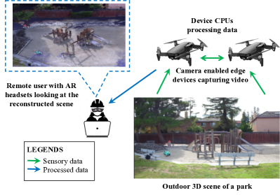
Figure 1: 3D reconstruction use case for areal reconstructed view of an outdoor scene using edge devices

Latency issues of 3D reconstruction: Unlike, simpler visual computing applications, SfM+MVS pipeline based 3D reconstruction methods, such as widely used openMVG/openMVS [3, 4] are extremely computation-intensive and thereby time-consuming even when performed within an edge environment. This is especially true for reconstructing large real-world scenes (mostly used during response for a emergency scene) that typically need $\geq 3$ high-resolution cameras to capture the target scene from different angles. This is due to the fact that such pipelines are traditionally designed to focus on the reconstruction accuracy and not the processing timeline. However, such high latency of reconstructing a 3D scene is counterproductive for disaster response as many involved missions such as area surveillance and reconnaissance multiple such compute-intensive applications run in sequence. In many of these missions, latency-sensitive applications such as AR/VR/MR, that run after the SfM+MVS based 3D reconstruction pipeline rely on the fast ($\leq 10$ s) and high quality reconstruction outcome for the success of the underlying missions (as shown in Fig. 1). Thus, there is a need to optimize such edge-supported 3D reconstruction pipeline’s latency without compromising the quality of the reconstruction outcome.

Challenges in balancing latency and quality: However, balancing the trade-off between latency and quality in resource-constrained edge devices is non-trivial as unintelligent application-agnostic quick-fixes can introduce additional challenges. For example:

• One possible approach to reduce the 3D reconstruction computation latency running on resource-constrained environments is to separate the dynamic but relatively smaller part (i.e., foreground) of the scene from the static but larger part (i.e., background) and frequently update this foreground to merge it with the less frequent background. However, this is challenging because the SfM pipelines always perform a bundle adjustment optimization, which has an inherent randomness that causes the results to fluctuate so that the foreground and background are located on different coordinate systems affecting the quality of the merged 3D model. Thus there needs to be intelligent application-side optimizations that are tailor made for the reconstruction pipeline.

• Another way to reduce the latency is to minimize data resolution and use a subset of cameras (i.e., video streams) in order to bring down the total data size for processing. However, on the flip side, unintelligent resolution degradation and camera selection can drastically reduce the 3D reconstruction quality, often rendering it useless. Thus, there is a need for intelligent edge system-side optimization that can balance the pipeline latency and reconstruction quality based on MEC resource availability.

• Finally, one of the important prerequisites for such delicate balancing act is the ability to efficiently (in terms of time) and effectively measure reconstruction quality. Quality evaluation needs to be time-efficient so that it can run in parallel to the reconstruction pipeline without eating into the latency savings from application- and system-side optimizations. This in turn makes effective quality evaluation tricky as most state-of-art evaluation techniques [5, 6, 7] assume the availability of ground truth which might not be practical when such evaluations need to be lightweight and quick. Contrarily, the absence of ground truth makes the systematic evaluation of 3D reconstruction challenging.

Thus overall, in order to effectively perform latency optimizations that do not impact the reconstruction quality, it is of paramount importance that such optimizations are customized towards the 3D reconstruction task pipeline and the underlying algorithms.

Our contributions: In order to address the aforementioned challenges, we propose a latency optimized multi-view 3D reconstruction framework running on a collaborative MEC environment for disaster response that aims to balance the processing time and reconstruction quality. Particularly:

• In order to reduce processing complexity and thereby latency we introduce data-level parallelism by modifying the SfM+MVS pipeline to create separate pipelines for high frequency foreground reconstruction and low frequency background reconstruction. Through this, we avoided the redundant computation of the static part of the data and ensure MEC resource and time saving.

• We propose a lightweight MEC system optimization algorithm that can select the best configuration of reconstruction latency and quality (that satisfies user expectations) based on resource availability by adjusting the frames’ resolution and selection of cameras.

• As part of the MEC system-side optimizations, we propose a novel and lightweight camera selection algorithm in order to select an optimal set of cameras that best covers the target scene. In addition, the proposed algorithm can return a different set based on the desired number of cameras for optimization.

• We also propose an online reconstruction quality evaluation model that along with optimal configuration selection, and camera selection algorithms run in parallel to the optimized SfM+MVS pipeline as part of a novel inter-edge collaboration architecture implementing task-level parallelism.

• We evaluate the performance of our optimized framework on a hardware testbed with publicly available Dance1 and Odzemok from CVSSP-3D Project Sample Datasets [8]. Our results show that the proposed optimized framework can save the end-to-end processing time by $54\%$ for data sets Dance1 and Odzemok. We also conclude that the quality degradation caused by such parallelism is $4-7$%. The results demonstrate high adaptability and efficiency in optimizing the system objective. The proposed online algorithm can successfully handle different user requirements during a disaster response mission based on the availability of the MEC resources.

Paper organization: In rest of the paper, Section II discusses the related work and background on 3D reconstruction technique and openMVG/openMVS pipeline. Section III presents the system model and benchmarking experiments. Section IV discusses the application and system optimizations. Section V presents the evaluation method and experimental results. Section VI concludes the paper.

II Related Work

Accelerated 3D reconstruction: There are a few methods that attempted to optimize the latency of the aforementioned 3D reconstruction pipeline. Authors in [9] sort the images based on the spatial orders of the cameras ensuring large overlaps between two subsequent images of the ordered set. This helps to reduce the computation cost in the feature matching step. In [10], the authors optimize the densify point cloud step with a quasi-dense feature matching approach and achieved 9% improvement in latency. Authors in [11] group the sparse 3D points into different clusters and processes each cluster separately for dense textured mesh generation. This helps them to reduce around 13% of the total processing time. Compared to these, our work intelligently divides the data into foreground and background regions to significantly reduce the processing time.

Video analytics: The performance (e.g., accuracy) of video analytics depends on the joint impact of various configurations. In [12], the authors propose a framework for both configuration adaptation and bandwidth allocation of edge-assisted video analytics. Authors in [13] jointly consider the interaction between accuracy, video quality, battery constraints, and network parameters to find an optimal offloading strategy. VideoStrom [14] optimizes query scheduling by exploring utility-based resource management in terms of query accuracy and delay; while VideoEdge [15] extends the problem to query placement across a hierarchy of clusters. Nevertheless, none of those works can be applied to the multi-view 3D reconstruction applications which is our focus in this paper.

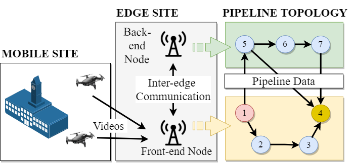
Figure 2: Disaster response system model of collaborative MEC architecture for multi-view 3D reconstruction pipelines

III System Model and Evidence Analysis

III-A System Model and Objectives

Fig. 2 shows the disaster response system model of our proposed collaborative MEC architecture implementing the openMVG/openMVS pipeline for end-to-end 3D reconstruction. Our system includes: 1) a group of synchronous video sequences of a scene offloaded by camera enabled edge devices, 2) a front-end edge device/node where the uploaded frames are initially stored and the main 3D reconstruction procedures are undergoing, 3) a back-end edge device/node (helper) which is executing the pipeline in parallel. The edge nodes are connected to each other through point to point wireless or wired link similar to typical real-world setups. In this paper, a video analytics task is defined as reconstructing a dense point cloud from the images captured at the same timestamp. We denote $\mathcal{I}=\{1,2,3...I\}$ as the set of reconstruction tasks for all the timestamps in offloaded videos. We assume that the user has an end-to-end processing deadline requirement and requires the best possible reconstruction quality, both calculated as an average of multiple frames. Based on such real-world use case assumptions, the objective of the MEC system is to maximize the average reconstruction quality while meeting the average processing deadline.

TABLE I: Processing latency and quality of openMVG/openMVS pipeline with varying camera resolution and camera selection

Metrics	Scale = 1, all cameras	Scale = 0.8, all cameras	Scale = 0.6, all cameras	Scale = 1, sans camera #0	Scale = 1, sans camera #2
Total latency	26.17 s.	16.07 s	9.1 s.	20.98 s.	19.83 s.
Number of Vertices	277,790	173.139	103,493	238,821	206,513

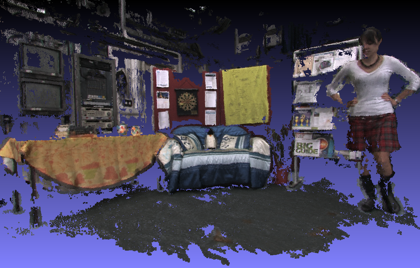
(a) With scale=1, all cameras

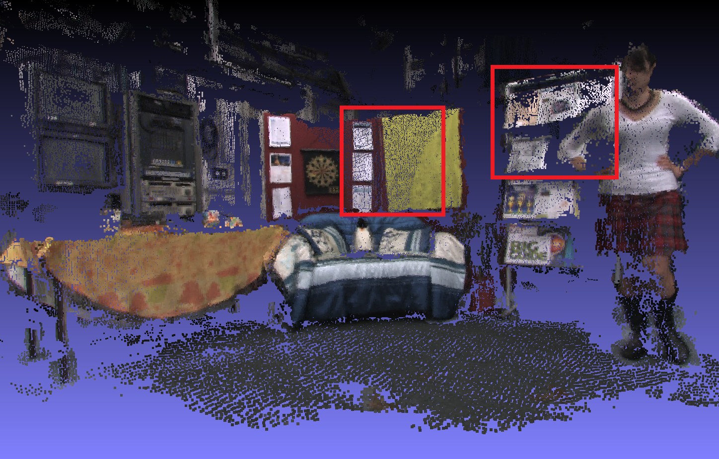
(b) With scale=0.6, all cameras

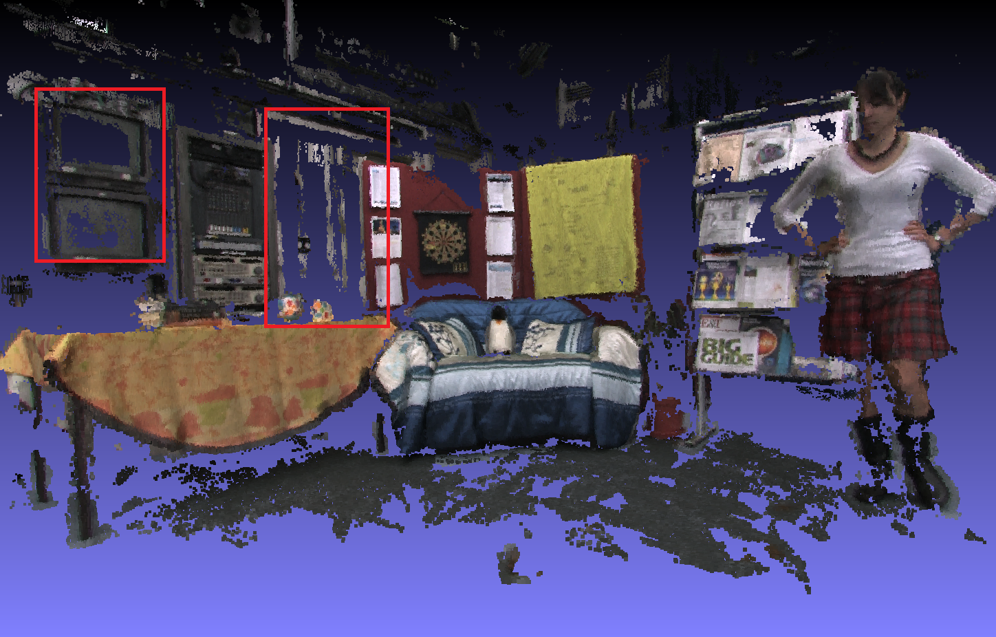
(c) Without scale=1, sans camera #2

Figure 3: Qualitative analysis of openMVG/openMVS pipeline with varying camera resolution and selection

III-B Problem Evidence Analysis

Here, we use qualitative and quantitative experimental results to demonstrate the effects of frame resolution and the number of cameras on 3D reconstruction pipeline latency and quality in order to motivate the need for intelligent application- and system-side optimizations. We use publicly available Dance1 [8] dataset (7 synchronous video sequences from static cameras) on a Dell desktop with Intel i7 @2.9GHz processor with 16GB RAM for the benchmarking experiments. The desktop used to some extent mimic the CPU capacity of a low-cost edge device.

Quantitative results: Here we investigate the effects of simple and ‘quick fix’ optimization strategies on processing latency. Table I demonstrates how openMVG/openMVS pipeline latency can be reduced by varying camera resolution and number of cameras for reconstruction. The table compares the latency of ideal configuration that includes all camera data with original resolution (scale = 1) against resolution compromised reconstructions. We observe that both the processing latency and the number of reconstructed vertices decrease as resolution decreases. This is because with lower resolutions, the images lose part of pixels during resizing. Table I also shows the impact of number of cameras and selection of cameras for reconstruction. In particular, we show the processing time comparison when we randomly remove camera $\#0$ and camera $\#2$ without altering the original resolution. The results demonstrate that the degree of such effect varies from camera to camera based on their orientation and coverage. For example, the effect of removing camera $\#2$ is greater than removing camera $\#0$ in terms of number of reconstructed vertices.

Qualitative results: The qualitative analysis shows that the aforementioned latency minimizing ‘quick fixes’ can adversely impact the quality of reconstructed 3D scene. Fig. 3(a) shows the golden results i.e., reconstruction with original resolution and all camera images. Whereas Fig. 3(b) also uses all images but resizes images to scale $0.6$ (i.e., $60$% of the original resolution). Fig. 3(c) instead shows the reconstructed scene with original resolution images from all cameras but without images from camera #2. Visually, we can see that with lower resolution, the reconstructed scene is not as smooth and delicate as the golden result (highlighted in Fig. 3(b)). Similarly when using fewer images (i.e., without images from camera #2), the reconstructed scene is not as complete as the golden result (highlighted in Fig. 3(c)). The quantitative and qualitative results together motivate the need for intelligent optimizations towards meaningful reduction in reconstruction latency without significantly degrading quality.

IV Optimization Methodology

This section will discuss the overall optimization problem from two angles. First, we propose application-side optimizations involving background subtraction to reduce the processing time by removing repeated background information. Next, based on the application-side optimization outcome, we formulate a system optimization problem to address the trade-off between reconstruction quality and latency. This helps to find the optimal image resolution and the selection of cameras.

IV-A Application-side Optimizations

In this paper, we propose a parallelized pipeline on openMVG/openMVS platforms by segmenting a scene into foreground (dynamic part) and background sections that can be later exploited by system-side optimizations through the collaborative MEC environment. This is achieved by the sub-tasks described below and illustrated as flowchart in Fig. 4.

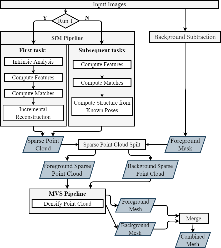
Figure 4: An overview of application implementation that runs parallel MVS pipelines for the foreground and background 3D reconstruction.

Background subtraction: We use openCV Background Subtractor to learn and subtract the static background model of a scene to identify the moving or dynamic regions. Since a scene can contain multiple moving objects, we used $k$-means clustering [16] with optimum cluster numbers to group the dynamic regions into clusters. Each of the clusters suggests a moving object. This helps us to create separate foreground masks (contiguous dynamic regions in the background subtracted binary image) when moving objects are spatially apart, thus reducing the foreground area to be 3D reconstructed.

Sparse point-cloud split: Since openMVS requires a lot of computation to generate the dense point cloud [4], our optimized pipeline uses foreground masks (obtained from background subtraction) to group the sparse 3D points (obtained from openMVG) into the foreground and background sets. This separation enables running openMVS pipeline separately and concurrently for foreground and background 3D reconstruction.

Merge foreground and background: Once the background and foreground 3D reconstruction results of consistent scale, translation, and rotation are stored in .ply files with the basic information of the 3D model such as, the number of 3D points and their locations and the color information of each point, we generate the full 3D map of the scene by combining the information stored in the .ply files.

IV-B System-side Optimizations

For system optimizations, we propose an online optimization framework to address the trade-off between quality and processing time by choosing optimal reconstruction configurations. This framework exploits the collaborative MEC environment to achieve task level parallelism.

Problem formulation: We define $\mathcal{N}=\{1,2,3,..N\}$ to be the set of cameras (i.e., edge devices for video capture), where $N\geq 3$. We create a binary camera-selection indicator $o_{n},\forall n\in\mathcal{N}$ i.e., $o_{n}=0$ indicates that the image from camera-$n$ will be ignored by the pipeline; otherwise $o_{n}=1$. We also denote $\Delta_{t}$ as the user’s (i.e., reconstruction task’s) deadline requirement. Based on the problem evidence analyses, we know that both the quality $Q$ and the processing latency/time $T$ are functions of camera/image resolution $r\in[r_{min},r_{max}]$ and camera subset $\mathcal{N}^{\prime}\subseteq\mathcal{N}$, i.e., $Q(r,\mathcal{N}^{\prime})$ and $T(r,\mathcal{N}^{\prime})$. With such settings, our optimization problem can be stated as:

$$\max_{r,\mathbf{o}} \;Q(r,\mathcal{N}^{\prime})$$ (P1)

s.t.  C1: $$r\in[r_{min},r_{max}]$$

C2: $$o_{n}\in\{0,1\},\;\forall n\in[1,N]$$

C3: $$\sum\limits_{n=1}^{N}o_{n}\geq 3,\;\forall n\in[1,N]$$

C4: $$T(r,\mathcal{N}^{\prime})\leq\Delta_{t}$$

where constraints C1 and C2 restrict the selection of camera resolution and number respectively, C3 specifies that the number of cameras should be at least 3 (required by openMVG [3]), and C4 specifies that the processing time needs to satisfy the user’s deadline requirement $\Delta_{t}$. Problem P1 is non-trivial to solve as: 1) Firstly, it is time-consuming to create accurate mathematical models (such as by taking massive measurements [12]) for quality $Q(r,\mathcal{N}^{\prime})$ and processing time $T(r,\mathcal{N}^{\prime})$ and 2) Secondly, the camera indicators are binary variables and the number of camera subset is very large (i.e., $\mathcal{O}(2^{N}$)). Therefore, computing all the solutions in this massive configuration space at run-time will be counterproductive.

Camera selection algorithm: In order to reduce the complexity of (P1), we propose a camera selection algorithm to select the $N^{\prime}$ most useful cameras. However, the camera selection scheme with 3D reconstruction is quite different from the typical maximal coverage problems [17] as in 3D reconstruction, the reconstructed points must be covered by at least two cameras. In this algorithm, the 3D points and their corresponding cameras are first extracted from the SfM pipeline. With these, our objective is to choose the cameras that will result in the maximum number of 3D points that are covered by at least two cameras. The most trivial way to do this is to implement a brute force technique; however, that will cause the running time to grow exponentially with the increase in number of cameras. Therefore, we develop the following optimization problem:

$$\max \sum_{k=1}^{\mathbb{P}}p_{k}$$ (P2)

s.t.  C1: $$\sum_{n=1}^{N}o_{n}=N^{\prime}$$

C2: $$M_{kn}=c_{n}A_{kn},\;\forall n\in[1,N],\;\forall k\in[1,\mathbb{P}]$$

C3: $$\sum_{n=1}^{N}M_{kn}\geq 2p_{k},\;\forall k\in[1,\mathbb{P}]$$

In (P2), we assume that there are a total of $\mathbb{P}$ 3D points and $N$ cameras and out of them $N^{\prime}$ cameras are chosen. $p_{k}$ is a binary variable which is 1 if 3D point-$k$ is covered by at least two chosen cameras and $0$ otherwise. Thus the objective function is to maximize the points that are covered by at least two cameras. The constraint C1 states that a total of $N^{\prime}$ cameras are chosen. Also, we assume that $A_{kn}$ is a known binary variable that is 1 if point-$k$ is covered by camera-$n$ and 0 otherwise; and $M_{kn}$ is a binary variable that is 1 if (a) point-$k$ is covered by camera-$n$, and (b) camera-$n$ is chosen, which is ensured by constraint C2. Constraint C3 ensures that point-$k$ is covered by at least two chosen cameras. We use Gurobi solverto solve (P2). As the number of 3D points is pretty large in a complex image, we first choose a small fraction of key points using $k$-means algorithm, and apply (P2) with these key-point subset to choose the most useful cameras.

1 Initialization: Set $N^{\prime}=N$, $r_{min}=0.3$, $r_{max}=1.0$, $r^{*}=1.0$;

2 Run the first task with $(r^{*},\mathcal{N})$, solve P2 and initial $\pi(N^{\prime}):N^{\prime}\rightarrow\mathcal{N^{\prime}}$;

3 $r=r_{min}$, $solutions=[]$;

4 $optimization$ = True;

5 for each upcoming task $i\in\mathcal{I}$ do

6       Observe $T(r,\pi(N^{\prime}))$, $Q(r,\pi(N^{\prime}))$

7       if not $optimization$ then

             do minor-adjustment ;

              // see section IV-B

8             continue

9      if $T(r,\pi(N^{\prime}))\leq\Delta_{t}$ then

10             $r_{min}=r$;    $r^{*}=r$;   

             $solutions$ $\leftarrow$ [$Q(r,\pi(N^{\prime}))$] ;

              // stores the current optimal configurations

11            

12      else

13             $r_{max}=r$;

14      if $r_{max}-r_{min}\leq\tau$ then

             $r_{min}=r^{*}$;    $r_{max}=1.0$;   $r=r_{min}$;   $N^{\prime}=N^{\prime}-1$;

              // another level of search

15             if $N^{\prime}<3$  then

16                   $r^{*},{N^{\prime}}^{*}=\operatorname*{arg\,max}(Q(r,\pi(N^{\prime})))$ in $solutions$ $optimization$ = False;

17            

18      else

19             $r=(r_{max}+r_{min})/2$

20      

Algorithm 1 Online Bi-section search algorithm

Transformation of P1 and solution: After solving (P2), we create a mapping function $\pi(N^{\prime}):N^{\prime}\rightarrow\mathcal{N^{\prime}}$ that specifies the unique mapping between the number of cameras and the selection of camera subset, i.e., given the number of cameras $N^{\prime}$, the selection of $\mathcal{N^{\prime}}$ is fixed. This function greatly reduces the domain size of (P1). Therefore, (P1) transforms to:

$$\max_{r,N^{\prime}} \;Q(r,\pi(N^{\prime}))$$ (P3)

s.t.  C1: $$r\in[r_{min},r_{max}]$$

C2: $$N^{\prime}\in[3,N]$$

C3: $$T(r,\pi(N^{\prime}))\leq\Delta_{t}$$

In (P3), $Q(r,\pi(N^{\prime}))$ and $T(r,\pi(N^{\prime}))$ are still unknown to the MEC system. However, by fixing one of the two parameters (e.g., $Q(r|\pi(N^{\prime}))$, $T(r|\pi(N^{\prime}))$ and $Q(\pi(N^{\prime})|r)$, $T(\pi(N^{\prime})|r)$), we can easily get that the quality and the processing time are monotonic functions of both $r$ and $N^{\prime}$. Therefore, the problem can be effectively solved by a two-dimensional Bi-section algorithm. The algorithm is driven by online observations that is described in Algorithm 1.

In Algorithm 1, we perform multiple Bi-section searches; the goal of each Bi-section is to find the optimal resolution $r^{*}$ for a given camera subset $\pi(N^{\prime})$. We assume the minimum resolution $r_{min}$ to be 0.3. The algorithm starts with a default configuration $(r=r_{min},\pi(N^{\prime}=N))$ (lines 3-4). For each upcoming task, the MEC system first runs the pipeline and observes the processing time $T(r,\pi(N^{\prime}))$ and quality $Q(r,\pi(N^{\prime}))$ (line 6). In lines 10-21, the algorithm compares the current processing time to the deadline $\Delta_{t}$ and performs Bi-section search on the resolution for the current camera subset $\pi(N^{\prime})$. In the meantime, it stores the current optimal configurations $(r^{*},\pi(N^{\prime}))$ and the corresponding quality into $solutions$ vector (line 12). In lines 15-16, when the search on current camera subset be finished, the algorithm resets the $r_{min}$ to the current optimal resolution $r^{*}$. Next it goes into the next Bi-section search on camera subset $\pi(N^{\prime}=N^{\prime}-1)$. This process terminates when $N^{\prime}<3$ or $r_{max}-r_{min}\leq\tau$, where $\tau$ is a constant which is assumed to be 0.01.

We also add the following functions to further reduce the time complexity during the configuration exploration.

1. Baseline_check: If $T(r_{min}|\pi(N^{\prime}_{i}))>\Delta_{t}$, stop Bi-section search on $N^{\prime}_{i}$ and go to $N^{\prime}_{i}-1$. This means that the processing of the lowest resolution has exceeded the deadline and there is no need to further explore $N^{\prime}_{i}$, i.e., $T(r^{\prime}|\pi(N^{\prime}_{i}))>T(r_{min}|\pi(N^{\prime}_{i}))$, $\forall r^{\prime}>r_{min}$.

2. Given $N^{\prime}_{i}<N^{\prime}_{j}$, if there exists a feasible solution ($r^{*}_{j},N^{\prime}_{j}$) and $Q(r_{max}|\pi(N^{\prime}_{i}))\leq Q(r_{j}^{*}|\pi(N^{\prime}_{j}))$, terminate optimization. The reason being $Q(r_{max}|\pi(N^{\prime}_{k}))\leq Q(r_{j}^{*}|\pi(N^{\prime}_{j}))$, $\forall N^{\prime}_{k}<N^{\prime}_{j}$.

3. Given $T(r|\pi(N^{\prime}_{i}))>\Delta_{t}$, if there exists a feasible solution ($r^{*}_{j},N^{\prime}_{j}$) and $Q(r|\pi(N^{\prime}_{i}))\leq Q(r_{j}^{*}|\pi(N^{\prime}_{j}))$, stop Bi-section search on $N^{\prime}_{i}$ and go to $N^{\prime}_{i}-1$. The reason being $Q(r^{\prime}|\pi(N^{\prime}_{i}))\leq Q(r_{j}^{*}|\pi(N^{\prime}_{j}))$, $\forall r^{\prime}<r$.

Minor-adjustment procedure: We add a minor-adjustment procedure (line 8 in Algorithm 1) to solve the problem of processing time fluctuation between consecutive tasks and facilitate the average processing time to converge to $\Delta_{t}$. At a given timestamp $I^{\prime}\leq I$, the adjustment rule follows:

$$r^{*}\text{=}\begin{cases}r^{*}+\tau&{1\over I^{\prime}}\sum\limits_{i=0}^{I^{\prime}}T_{i}(r^{*})<\Delta_{t}\;\&\;T_{i}(r^{*})<\Delta_{t}\\ r^{*}-\tau&{1\over I^{\prime}}\sum\limits_{i=0}^{I^{\prime}}T_{i}(r^{*})>\Delta_{t}\;\&\;T_{i}(r^{*})>\Delta_{t}\\ r^{*}&\text{otherwise}\end{cases}$$ (1)

Based on the difference between current average processing time and deadline, we slightly decrease or increase $r^{*}$ by $\tau$ (e.g., 0.02).

Background update strategy: As explained in Section IV-A, the application-side optimization through background subtraction updates the foreground frequently and therefore is reconstructed for each task. However, the background reconstruction is significantly more time consuming and computationally intensive. Thus, a continuous background reconstruction in parallel to foreground is only going to lengthen the overall processing time. Contrarily, the polar opposite method of performing the background reconstruction only once during the entire reconstruction lifecycle can benefit processing latency; however, might significantly degrade the reconstruction quality. To address this issue, we let the front-end node of the collaborative MEC environment to continuously reconstruct the foreground and the back-end edge node to opportunistically perform background reconstruction only during its idle time (denoted by $\Delta_{a}$ as shown in Fig 5). The newly reconstructed background result will be actively pushed to the front-end node.

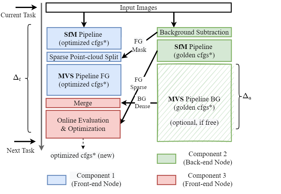
Figure 5: An overview of the collaborative MEC environment running the optimized pipeline

Overall system implementation: The resulting optimized framework implementation with all application-side and system-side optimization steps on the collaborative MEC environment is illustrated in Fig. 5. First, the front-end node performs “SfM Pipeline” with optimized configurations, while the back-end node simultaneously executes “Background Subtraction” and sends the foreground masks to the front-end node. Once it gets the foreground masks, the front-end node starts “Sparse Point-cloud Split” and “MVS pipeline FG” to create the dense foreground point-cloud, and then merges it with the existing background point-cloud. During the same time, the back-end node performs the “SfM pipeline” with golden configurations, and the result is sent to the front-end node for “Online Evaluation $\&$ Optimization” (we discuss online evaluation in detail in Section V-A). Beyond that, the back-end node uses spare time to reconstruct the background until the next task arrives as explained in Section IV-A. The processing latency of the proposed pipeline depends on the length of its ‘critical path’, which is the time elapsed between component 1 and component 3.

TABLE II: Foreground F-score comparison between online and offline evaluations

F-score	Scale=0.95	Scale=0.90	Scale=0.85	Scale=0.80	Scale=0.75	Scale=0.70
After openMVG (online evaluation)	0.911	0.888	0.873	0.864	0.855	0.819
After openMVS (offline evaluation)	0.873	0.851	0.836	0.817	0.797	0.770

V System Evaluation and Results

In this section, we evaluate the performance of the proposed optimized framework and validate our online quality evaluation method through experiments on a hardware edge testbed with real datasets. The hardware MEC testbed mostly mimics the system model from Fig. 2 and consists of a front-end node (Dell desktop equipped with Intel i7-10700F @2.9GHz, 16GB RAM) and a back-end node (Dell desktop equipped with Intel i7-10700k @3.8GHz, 32GB RAM). These mimic low cost edge devices with no GPU capability. The two nodes are connected via 10 Gbps Ethernet cable mimicking point to point connectivity between the nodes. The video datasets used for the evaluations are Dance1 and Odzemok [8].

V-A Evaluation Method

For offline qualitative evaluation, i.e., to test the performance of our optimized pipeline (without the concern of evaluation latency), we use the metric proposed in [18]. In this method, the quality is measured in terms of precision ($P$), recall ($R$), and F-score ($F$) - where $P$ measures how close a 3D point cloud is to the ground truth, $R$ measures the completeness of the reconstruction, and $F$ is a function of $P$ and $R$, i.e. ,

$$F={2PR\over(P+R)}$$

In this paper, we select distance threshold $d$ = 0.01 mm, 0.02 mm to determine whether a point from the reconstructed point cloud and a point from the ground truth are close enough. However, due to the lack of ground truth, we run the original openMVG/openMVS pipeline to reconstruct a 3D model with the best configuration (i.e., original resolution at scale=1 and with all cameras). This golden result (as explained in Section III) is our best estimate of the ground truth and thus is used to calculate the F-score of the reconstructed outcome of our optimized pipeline.

V-B Validity of Online/Run-time Quality Evaluation

One of the trickiest aspects of our optimized pipeline is to measure the quality $Q(r,\pi(N^{\prime}))$ of 3D reconstruction online, i.e., in runtime and use this outcome to ascertain optimal configurations for next task. In order to achieve this, we perform the evaluation on the foreground sparse point cloud obtained from openMVG’s SfM pipeline instead of the mesh from openMVS (as shown in Fig. 5) due to the fact that: i) the former is the foundation of the latter; ii) openMVS steps often take more time; and iii) the foreground is more important and always changing. Whereas, for the offline qualitative evaluations explained in Section V-A, we take the more traditional approach of comparing the foreground mesh from openMVS against the foreground from golden result. In order to establish the validity of the proposed online evaluation by establishing positive correlation between the online and offline evaluations, we compare the F-scores values of foreground after openMVG’s SfM against foreground after openMVS in Table II. The results show that for both cases F-scores decrease as resolution decreases. Furthermore, their decreasing trends are also comparable. Therefore, we believe that our proposed online evaluation is a valid methodology that successfully reflects the quality of the 3D reconstruction of our optimized pipeline.

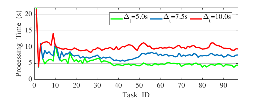
Figure 6: Task processing time deadline satisfaction

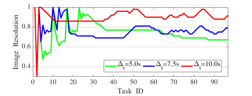
Figure 7: Resolution adaptation.

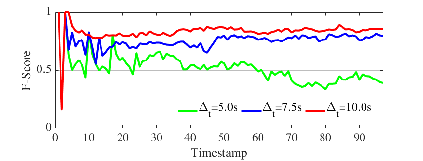
Figure 8: F-score (foreground only).

V-C Optimization Evaluation

Given a processing deadline $\Delta_{t}$, here we evaluate the outcome of the online optimization and background update strategy in terms of average task processing time and reconstruction quality $Q(r,\pi(N^{\prime}))$ (using F-score). Taking into account that the processing time $T(r,\pi(N^{\prime}))$ of the pipeline can vary according to the content of the input images, we accept a small margin of error during the configuration searching steps (based on experimental results, the margin is set to 1s). Specifically, a configuration is considered as acceptable if $0<|\Delta_{t}-T(r,\pi(N^{\prime}))|\leq 1$. In this evaluation, the deadlines $\Delta_{t}$ of test cases are 5.0s, 7.5s and 10.0s, respectively.

Fig. 6 shows the processing time of individual tasks at different timestamps. Driven by the minor-adjustment procedure that we proposed in subsection IV-B, we notice that the processing time gradually converges to the pre-defined deadline $\Delta_{t}$ after the optimal configuration is found. The results of optimal configuration search (Alg. 1) and subsequent resolution adaptation (minor-adjustment procedure) are shown in Fig. 7. As the system takes more configuration search steps to find the optimal number of cameras for tasks with shorter deadline, the figure demonstrates that the image resolution of tasks with longer deadline (e.g., $\Delta_{t}=7.5s$ and $\Delta_{t}=10.0s$) converges faster than tasks with shorter deadline (e.g., $\Delta_{t}=5.0s$). Fig. 8 shows the quality distribution $Q(r,\pi(N^{\prime}))$ (in terms of F-scores) of the foreground. After some initial randomness while the online optimization algorithm is still running, the F-score values of foreground sparse 3D point-cloud start to converge once the minor adjustment procedure starts to work. Such convergence behavior of F-score under different task deadlines is similar to resolution adaptation (as shown in Fig. 7). The overall statistical outcome in terms of chosen configuration along with average processing time, average F-score, background update and number of search steps are presented in Table III.

TABLE III: Online optimization with different deadlines - Dance1

Info	Deadline ($\Delta_{t}=5s$)	Deadline ($\Delta_{t}=7.5s$)	Deadline ($\Delta_{t}=10s$)
Avg. Resolution Scale	0.74	0.76	0.90
$\#$ Cameras	4	7	7
Avg. Processing Time	5.28 s	7.49 s	9.98 s
Avg. F-score of FG	0.51	0.74	0.83
$\#$ Reconstructed BG Dense Point Clouds	22	36	54
$\#$ Configuration Search Steps	27	12	1

While evaluating the performance of the background update strategy discussed in Section IV-B, we observe that for datasets such as Dance1, the system only needs to create a background model once as the background scene remains unchanged. However, for real-world scenarios where background scene may change frequently, it is beneficial to use up-to-date background model. Upon monitoring the speed of background update for dataset Dance1 (with different processing deadlines), we observe that the back-end node can generate a new background point cloud around $20-25$s without interrupting the foreground reconstruction. Moreover, the background update frequency of tasks with larger deadline is much higher than tasks with shorter deadline. For example, the number pushed background dense point clouds are 22, 36 and 54 when the task deadline is set to $\Delta_{t}=5s$, $\Delta_{t}=7.5s$ and $\Delta_{t}=10s$, respectively. This can be explained by Fig. 5 i.e., larger deadline $\Delta_{t}$ leads to larger $\Delta_{\alpha}$. In other words, while the front-end node is busy running foreground reconstruction with some high configurations, the back-end edge node has more idle time to perform background reconstruction. The above results indicate that the proposed online algorithm (Algo. 1) and optimized pipeline (Fig. 5) can effectively balance the trade-off between latency and quality.

TABLE IV: Quality comparison between original and optimized pipeline

F-score	Threshold $d=0.01$	Threshold $d=0.02$
Optimal Dance1	avg F-score = 0.930 std = 0.026	avg F-score = 0.961 (std = 0.019)
Optimal Odzemok	avg F-score = 0.946 (std = 0.012)	avg F-score = 0.967 (std = 0.011)

V-D Quality and Latency Evaluation

Finally, we compare the quality and latency results of our optimized pipeline against the golden results of the original pipeline for both the datasets. For the quality comparisons, we run both pipelines with the same input images and compute F-score - when construct with original resolution and all camera data. The F-score for the optimized pipeline is calculated by assuming the golden results (i.e., from original pipeline) as ground truth. Table IV shows the average F-scores and standard deviation for each of the datasets. Overall, we can conclude that reconstruction quality from our optimal pipeline are within $4-7$% of the peak quality (from Table IV) which is negligible for successful operation of other AR/VR/MR applications that typically run after reconstruction pipeline. However, when we compare the latency results of our optimized pipeline against original pipeline (as shown in Table V), we see that the average improvement for datasets Dance1 and Odzemok is around $54\%$ (we notice that such improvements depend on the number of pixels contained in the foreground areas). Inferring from all the results, we argue that our proposed pipeline (as shown in Fig. 4 and Fig. 5) can significantly lower down the processing latency at the cost of very limited quality degradation. Therefore, such improvement can greatly help latency-sensitive applications whose quick turnaround time and high quality results drive the success of the underlying disaster response mission.

TABLE V: Latency comparison between original and optimized pipelines

Step	Original Dance1	Optimal Dance1	Original Odzemok	Optimal Odzemok
SfM Pipeline (optimized cfgs)	-	2.94 s	-	3.01 s
MVS Pipeline of FG	-	8.78 s	-	5.67 s
Others (Split, Merge)	-	0.26 s	-	0.21 s
Total Time	26.17 s	11.98 s (54.22%)	19.43 s	8.89 s ($54.25\%)$

VI Conclusions and Future Work

In this paper, we developed a collaborative MEC architecture for disaster response based on an optimized framework that balances the trade-off between 3D reconstruction processing latency and quality. By exploiting the data and task level parallelism, our optimized edge-supported framework achieves a significant reduction in end-to-end latency, with negligible loss in reconstruction quality. In the future, we would like to extend this work on multiple fronts. One of the key limitations of our work is that the overall latency is still in tens of seconds when implemented on low cost compute devices. However, such latencies might not be acceptable for some real-world use cases (also restricted by use of limited CPU/GPU resources) that require real-time (i.e., $<$ 100 ms) response. Therefore, one of our future research directions is to reduce the end-to-end latency even further using algorithmic optimization that uses deep learning based methods and models.

References

- [1] “Smart emergency response system (sers),” http://smartamerica.org/.
- [2] X. Zhang et al., “Effect: Energy-efficient fog computing framework for real-time video processing,” in IEEE/ACM CCGrid, 2021, pp. 493–503.
- [3] P. Moulon et al., “OpenMVG: Open multiple view geometry,” in RRPR, 2016, pp. 60–74.
- [4] D. Cernea, “OpenMVS: Multi-view stereo reconstruction library,” https://github.com/cdcseacave/openMVS, 2020.
- [5] Z.-H. Feng et al., “Evaluation of dense 3d reconstruction from 2d face images in the wild,” in IEEE FG, 2018, pp. 780–786.
- [6] H. Fan et al., “A point set generation network for 3d object reconstruction from a single image,” in IEEE CVPR, 2017, pp. 605–613.
- [7] S. M. Seitz et al., “A comparison and evaluation of multi-view stereo reconstruction algorithms,” in IEEE CVPR, vol. 1, 2006, pp. 519–528.
- [8] A. Mustafa et al., “General dynamic scene reconstruction from wide-baseline views,” in ICCV, 2015.
- [9] L. Lou et al., “A cost-effective automatic 3d reconstruction pipeline for plants using multi-view images,” in Conference Towards Autonomous Robotic Systems, 2014, pp. 221–230.
- [10] L. Wang et al., “An improved patch based multi-view stereo (pmvs) algorithm,” in International Conference on Computer Science and Service System, 2014, pp. 9–12.
- [11] J.-A. Wang et al., “Fast 3d reconstruction method based on uav photography,” ETRI Journal, vol. 40, no. 6, pp. 788–793, 2018.
- [12] C. Wang et al., “Joint configuration adaptation and bandwidth allocation for edge-based real-time video analytics,” in IEEE INFOCOM, 2020, pp. 1–10.
- [13] X. Ran et al., “Deepdecision: A mobile deep learning framework for edge video analytics,” in IEEE INFOCOM, 2018, pp. 1421–1429.
- [14] H. Zhang et al., “Live video analytics at scale with approximation and delay-tolerance,” in USENIX NSDI, 2017, pp. 377–392.
- [15] C. Hung et al., “Videoedge: Processing camera streams using hierarchical clusters,” in IEEE/ACM SEC, 2018, pp. 115–131.
- [16] S. Lloyd, “Least squares quantization in pcm,” IEEE Transactions on Information Theory, vol. 28, no. 2, pp. 129–137, 1982.
- [17] R. Wei et al., “Continuous space maximal coverage: Insights, advances and challenges,” Computers & operations research, vol. 62, pp. 325–336, 2015.
- [18] S. Ruano et al., “A benchmark for 3d reconstruction from aerial imagery in an urban environment.”