Characters, Quasinormal Modes, and Quantum de Sitter Thermodynamics

Abstract

In this short note, we review some recent progress in understanding the 1-loop corrections to the Gibbons-Hawking entropy, which amounts to studying free fields on the de Sitter static patch and the round sphere. After briefly surveying the unitary irreducible representations of the de Sitter group $SO(1,d+1)$ and their Harish-Chandra characters, we discuss the Lorentzian interpretation for the 1-loop sphere path integral for a scalar. After that we comment on how the results are modified by edge contributions for spinning fields.

1 Introduction

Due to the exponential cosmic expansion, the causal diamond for an inertial observer in a de Sitter (dS) spacetime $dS_{d+1}$ covers only a part of it known as the static patch, described by the metric

$$ds^{2}=-\left(1-\frac{r^{2}}{\ell_{\text{dS}}^{2}}\right)dt^{2}+\frac{dr^{2}}{1-\frac{r^{2}}{\ell_{\text{dS}}^{2}}}+r^{2}d\Omega_{S^{d-1}}^{2}\;.$$ (1)

The dS length $\ell_{\text{dS}}$ is related to the cosmological constant $\Lambda>0$ through $\ell_{\text{dS}}=\sqrt{\frac{d(d-1)}{2\Lambda}}$. Sitting at $r=0$, the observer is surrounded by a cosmological horizon of area $A_{c}=\ell_{\text{dS}}^{d-1}\text{Vol}(S^{d-1})$ at $r=\ell_{\text{dS}}$. A semiclassical analysis tells us that this horizon has a Hawking temperature $T_{\text{dS}}=\frac{1}{2\pi\ell_{\text{dS}}}$ and an associated Gibbons-Hawking entropy [1] (from now on we set $\ell_{\text{dS}}=1$)

$$S_{\text{GH}}=\frac{A_{c}}{4G_{N}}\;,$$ (2)

whose microscopic origin remains a mystery.

In the absence of a microscopic explanation, a bottom-up approach would to be study the quantum corrections to (2) in the low energy effective theory of gravity plus matter. These corrections provide unambiguous data testing candidate models, in similar spirit of that in the context of black hole microstate counting [2, 3, 4, 5, 6] and Higher-spin/CFT dualities [7, 8, 9, 10]. As an illustration, let us say one asserts that the dS horizon entropy $\mathcal{S}_{\text{macro}}$ for 3D pure gravity (computed in [11]) counts the number $W(N)$ of partitions of $N$. Both the macroscopic and microscopic entropies can be brought uniquely into an expansion of the form

$$\mathcal{S}_{\text{macro}}= \mathcal{S}_{0}-3\log\mathcal{S}_{0}+\cdots$$

$$\mathcal{S}_{\text{micro}}\equiv \log W(N)=\mathcal{S}_{0}-2\log\mathcal{S}_{0}+\cdots\;.$$ (3)

The failure to reproduce $\mathcal{S}_{\text{macro}}$ immediately falsifies the asserted microscopic proposal. In contrast, as shown in [12, 13], a $T\bar{T}(+\Lambda_{2})$-deformed $\text{CFT}_{2}$ reproduces $\mathcal{S}_{\text{macro}}$ for 3D pure gravity up to the logarithmic correction.

This note reports some recent progress [11, 14, 15] in studying the 1-loop corrections to (2), which as reviewed in Section 2 comes from the quadratic fluctuations of gravitons and matter in the Euclidean path integral around the round $S^{d+1}$ saddle. These contribute to the full dS entropy as

$$\mathcal{S}_{\text{macro}}=\cdots+\underbrace{b\log\mathcal{S}_{0}+c}_{\text{1-loop}}+\cdots\;.$$ (4)

The logarithmic correction (i.e. the coefficient $b$) depends only on the massless spectrum while the finite part $c$ receives contributions from the full matter content.

In understanding the 1-loop corrections, a key role is played by the Harish-Chandra character of the de Sitter group $SO(1,d+1)$. Our goals in this note are two-fold: first, to explain how these mathematically defined objects lead to a Lorentzian interpretation of the 1-loop Euclidean path integral; second, to describe qualitatively new features as one extends the discussion to spinning fields. We will restrict ourselves to generic dimensions $d\geq 3$ to avoid discussing special features that only appear in $d<3$.

After setting up the problem in Section 2, we will do a quick survey for unitary irreducible representations (UIRs) of $SO(1,d+1)$ in Section 3. In Section 4, we introduce the $SO(1,d+1)$ Harish-Chandra character and explain its physics. We discuss in Section 5 generalizations to spinning fields, before we conclude in Section 6. As we aim to keep the discussion concise, many details for the derivations (including for example a careful treatment of UV-divergences) will be inevitably omitted. We refer the interested readers to the original work [11, 14, 15] for the complete detail.

2 What is the Lorentzian interpretation of the 1-loop sphere path integral?

Proposed by Gibbons and Hawking [16], the full dS entropy is computed by a Euclidean path integral with a positive cosmological constant $\Lambda$, integrating over all metrics $g$ and matter fields collectively denoted by $\Phi$:

$$\mathcal{S}=\log\mathcal{Z}\;,\qquad\mathcal{Z}=\int\mathcal{D}g\,\mathcal{D}\Phi\,e^{-S[g,\Phi]}\;,$$ (5)

expanded around the round sphere $S^{d+1}$ saddle. At tree level in Einstein gravity, one recovers the Gibbons-Hawking entropy (2). At 1-loop, one integrates the quadratic fluctuations around this saddle, which for a scalar is given by the functional determinant of a Laplace operator on the sphere (whose radius is set to 1)

$$Z_{\text{PI}}=\int\mathcal{D}\phi\,e^{-\frac{1}{2}\int_{S^{d+1}}\phi\left(-\nabla^{2}+m^{2}\right)\phi}=\det\left(-\nabla^{2}+m^{2}\right)^{1/2}\;.$$ (6)

Such a quantity is UV-divergent and is typically regulated by for example zeta-function [17] or heat kernel [18] regularization.

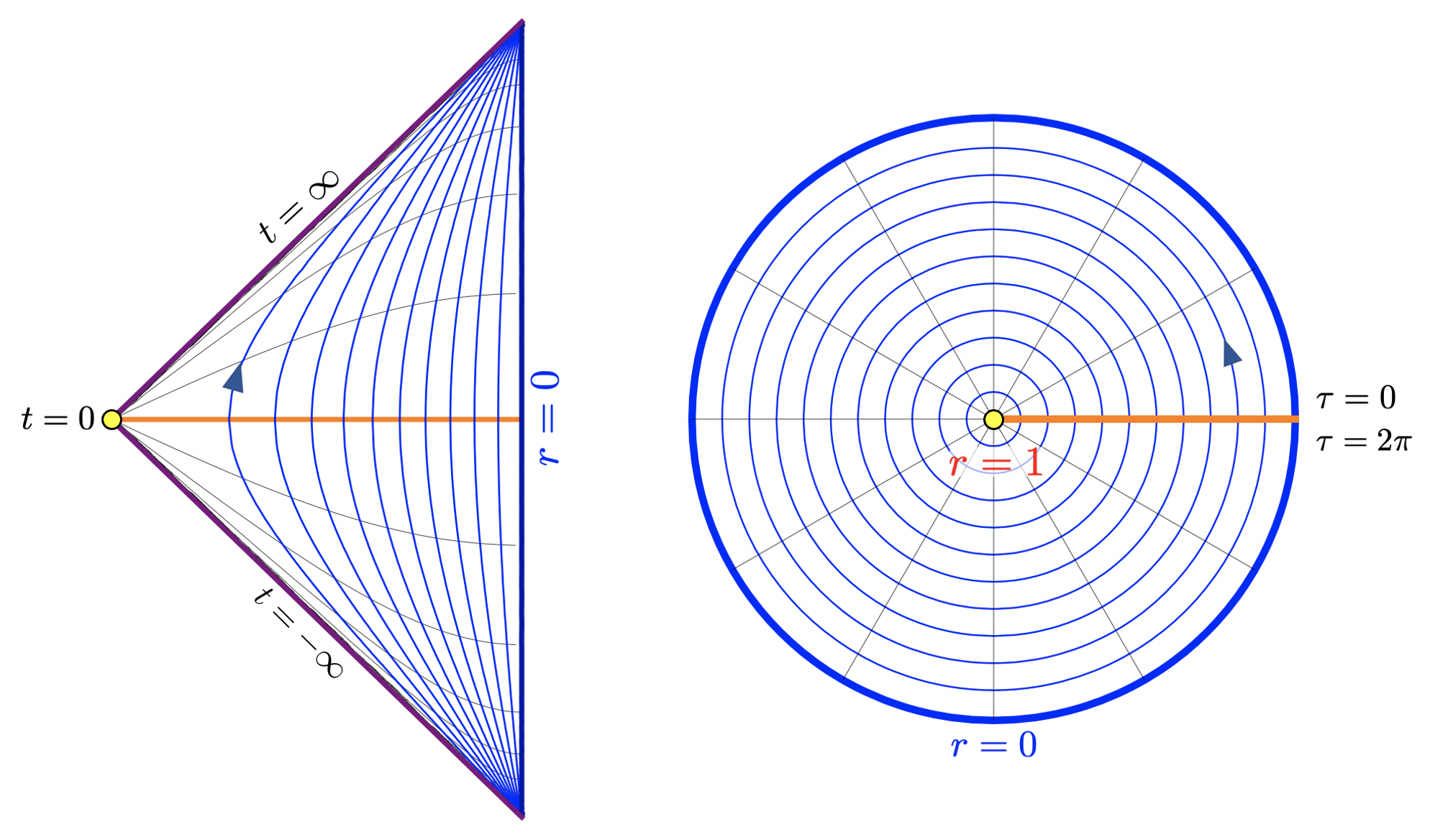
Figure 1: After Wick-rotating $t\to-i\tau$ and identifying $\tau\sim\tau+2\pi$, the dS static patch (left) turns into a sphere (right). The Euclidean time $\tau$ becomes an angular variable on the sphere. The horizon (yellow dot) at $r=1$ is mapped to the origin of the sphere.

Since $S^{d+1}$ can be obtained by Wick-rotating the static patch time $t\to-i\tau$ and identifying $\tau\simeq\tau+2\pi$ in (1) (see Fig.1), one expects that a 1-loop path integral on $S^{d+1}$ would have an interpretation as a thermal ideal gas canonical partition function for quantum fields living on a static patch at the dS temperature $T_{\text{dS}}=\frac{1}{2\pi}$. For a free massive scalar, this means

$$Z_{\text{PI}}\sim Z_{\text{bulk}}\equiv\text{``Tr"}\,e^{-2\pi\hat{H}}$$ (7)

where $\hat{H}$ is the static patch Hamiltonian with respect to which one defines positive energy modes, and “Tr"" is tracing over the associated Fock space. We use $\sim$ instead of an equal sign and put a quotation mark on Tr because the trace is in fact ill-defined. To see this, let us pretend that the spectrum of $\hat{H}$ were discrete. One could then compute the trace (7) by substituting the mode expansion for the scalar field and summing over occupation numbers, leading to

$$Z_{\text{bulk}}=\prod_{E>0}\frac{e^{-\pi E}}{1-e^{-2\pi E}}\;.$$ (8)

Here the product is over the discrete single-particle energy spectrum labeled by $E$; the factor $e^{-\pi E}$ is due to the zero-point energy for each positive-energy mode. Equivalently, we can write

$$\log Z_{\text{bulk}}=-\int_{0}^{\infty}d\omega\,\rho(\omega)\log\left(e^{\pi\omega}-e^{-\pi\omega}\right)$$ (9)

in terms of the single-particle density of states (DOS)

$$\rho(\omega)=\sum_{E>0}\delta(\omega-E)=\text{tr}\,\delta(\omega-\hat{H})$$ (10)

with tr tracing over the single-particle Hilbert space.

The trouble for us is that the spectrum of $\hat{H}$ is actually continuous, and the DOS $\rho(\omega)$ is strictly infinite. Physically, this is due to the fact that the horizon is an infinite redshift surface, enabling the existence of normal modes with arbitrary angular momentum and energy. Subsequently, expressions (8)-(10) do not make sense, casting doubts on the interpretation (7). What comes to rescue is the Harish-Chandra character for the de Sitter group $SO(1,d+1)$, which enables us to make sense of the right hand side of (7). Before explaining that, we will first quickly review the symmetries of $dS_{d+1}$ and the UIRs of the de Sitter group $SO(1,d+1)$.

3 Unitary irreducible representations of the de Sitter group $SO(1,d+1)$

3.1 The geometry of $dS_{d+1}$ and its symmetries

The $(d+1)$-dimensional dS space $dS_{d+1}$ can be thought of as a hyperboloid in $\mathbb{R}^{1,d+1}$

$$\eta_{AB}X^{A}X^{B}=-\left(X^{0}\right)^{2}+\left(X^{1}\right)^{2}+\cdots+\left(X^{d+1}\right)^{2}=1\;.$$ (11)

The hyperbloid (11) has a manifest $SO(1,d+1)$ isometry generated by Killing vectors $L_{AB}=X_{A}\partial_{X^{B}}-X_{B}\partial_{X^{A}}$, which satisfies the algebra

$$\left[L_{AB},L_{CD}\right]=\eta_{BC}L_{AD}-\eta_{AC}L_{BD}+\eta_{AD}L_{BC}-\eta_{BD}L_{AC}\;.$$ (12)

Defining

$$D=L_{0,d+1}\;,\quad M_{ij}=L_{ij}\;,\quad P_{i}=L_{d+1,i}+L_{0,i}\;,\quad K_{i}=L_{d+1,i}-L_{0,i}\;,$$ (13)

the algebra (12) is recast into the conformal algebra of $\mathbb{R}^{d}$:

$$[D,P_{i}]=P_{i}\;,\qquad[D,K_{i}]=-K_{i}\;,\qquad[K_{i},P_{j}]=2\delta_{ij}D-2M_{ij}\;,$$

$$[M_{ij},P_{k}]=\delta_{jk}P_{i}-\delta_{ik}P_{j}\;,\qquad[M_{ij},K_{k}]=\delta_{jk}K_{i}-\delta_{ik}K_{j}\;.$$ (14)

The static patch (1) corresponds to the intrinsic parametrization

$$X^{0}=\sqrt{1-r^{2}}\sinh t\;,\qquad X^{d+1}=\sqrt{1-r^{2}}\cosh t\;,\qquad X^{i}=r\,\Omega_{S^{d-1}}^{i}\;,$$ (15)

and has a manifest $SO(1,1)\times SO(d)$ symmetry corresponding to $t$-translation and rotations on $S^{d-1}$ generated by the boost $D$ and angular momentum $M_{ij}$ respectively. Other isometries of the global dS space, i.e. $P_{i}$ or $K_{i}$, do not preserve a single static patch but instead map different static patches into one another.

3.2 Particles in $dS_{d+1}$= UIRs of $SO(1,d+1)$

Analogous to Wigner’s classification of particles and fields in Minkowski spacetime by unitary irreducible representations (UIRs) of the Poincaré group, particles and fields in $dS_{d+1}$ are classified according to UIRs of the de Sitter group $SO(1,d+1)$. For an excellent review of the representation theory of $SO(1,d+1)$, we refer the reader to [19]. Here we will only do a quick survey for the dictionary between UIRs of $SO(1,d+1)$ and QFTs in $dS_{d+1}$.

A $SO(1,d+1)$ UIR $\mathcal{V}_{[\Delta,\mathbf{s}]}$ is labeled by an $SO(d)$ highest weight $\mathbf{s}=[s_{1},s_{2},\dots,s_{\lfloor\frac{d}{2}\rfloor}]$ and a conformal dimension $\Delta$; the former is nothing but the spin for the quantum field, while the latter is related to its mass. We focus on scalars and symmetric tensors, i.e. those with $\mathbf{s}=[s,0,\dots,0]$ and $s\geq 0$ is an integer. For a spin-$s$ field, its mass is related to the conformal dimension through

$$m^{2}=\begin{cases}\Delta(d-\Delta)\;,&s=0\\ (\Delta+s-2)(d+s-2-\Delta)\;,&s\geq 1\\ \end{cases}\;.$$ (16)

Unitarity requires that the generators (12) to act as anti-hermitian operators on the UIR $\mathcal{V}_{[\Delta,\mathbf{s}]}$, i.e.

$$L_{AB}^{\dagger}=-L_{AB}\;.$$ (17)

In terms of the conformal generators (13), these imply

$$D^{\dagger}=-D\;,\qquad P_{i}^{\dagger}=-P_{i}\;,\qquad K_{i}^{\dagger}=-K_{i}\;,\qquad M_{ij}^{\dagger}=-M_{ij}\;.$$ (18)

These conditions will restrict the form of the inner products (with respect to which one defines the hermitian conjugation) and the allowed values of $\Delta$. Note that (18) is distinct from the unitarity condition of the Lorentzian conformal group $SO(2,d)$ which demands for example $P_{i}^{\dagger}=K_{i}$, marking a fundamental difference between QFTs in de Sitter and anti-de Sitter space.

Principal series representations

These UIRs describe massive fields in $dS_{d+1}$ that are heavy compared with the dS scale $\ell_{\text{dS}}$. For a spin-$s$ field, its conformal dimension and mass fall into the ranges

$$\Delta=\frac{d}{2}+i\nu\;,\quad\nu\in\mathbb{R}\quad\Leftrightarrow\quad m\geq\begin{cases}\frac{d}{2}&\text{ for }s=0\\ s+\frac{d}{2}-2&\text{ for }s\geq 1\end{cases}\;.$$ (19)

Complementary series representations

These UIRs describe massive fields in $dS_{d+1}$ that are light compared with the dS scale $\ell_{\text{dS}}$. For a light scalar, it has

$$0<\Delta<d\qquad\Leftrightarrow\qquad 0<m<\frac{d}{2}\qquad(s=0)\;.$$ (20)

For a light spin-$s$ field, the ranges are instead

$$1<\Delta<d-1\qquad\Leftrightarrow\qquad\sqrt{(s-1)(s+d-3)}<m<s+\frac{d}{2}-2\qquad(s\geq 1)\;.$$ (21)

The lower bound $\sqrt{(s-1)(s+d-3)}$ is known as the Higuchi bound [20].

Exceptional series

These UIRs only exist for $s\geq 1$ and describe the so-called partially massless particles [20, 21, 22, 23, 24, 25, 26, 27, 28, 29, 30, 31]. These occur when the conformal dimension and mass hit the exceptional points

$$\Delta=1-p\qquad\Leftrightarrow\qquad m_{s,p}^{2}=(s-1-p)(d+s+p-3)\;,\qquad p=0,1,\dots,s-1\;,$$ (22)

The local action describing these fields have the gauge symmetry that reads schematically

$$\phi_{\mu_{1}\cdots\mu_{s}}\sim\phi_{\mu_{1}\cdots\mu_{s}}+\nabla_{(\mu_{s-p}}\cdots\nabla_{\mu_{s}}\xi_{\mu_{1}\cdots\mu_{p})}+\dots\;,$$ (23)

where $\cdots$ stand for terms with fewer derivatives [30]. We call the integer $p$ "depth", which is equal to the spin of the gauge parameter. In particular, the usual massless spin-$s$ field has depth $p=s-1$.

4 Harish-Chandra character of $SO(1,d+1)$ and its physics

A useful object to encode the information about a $SO(1,d+1)$ UIR is the Harish-Chandra character, defined as a trace of a group element over the representation space $\mathcal{V}_{[\Delta,\mathbf{s}]}$. The general theory for Harish-Chandra characters and their computations in the case of $SO(1,d+1)$ are reviewed in [19]. For our purpose, we will focus on the character for the group element generating time translation in the static patch

$$\chi_{[\Delta,\mathbf{s}]}(t)=\text{tr}_{[\Delta,\mathbf{s}]}\,e^{-i\hat{H}t}\;.$$ (24)

We have written in terms of $\hat{H}=i\hat{D}$, which can be interpreted as a hermitian Hamiltonian with a real spectrum. The character (24) has the property that $\chi_{[\Delta,\mathbf{s}]}(-t)=\chi_{[\Delta,\mathbf{s}]}(t)$. In the following discussion, we will restrict to $t>0$ unless specified.

Principal and complementary series

For these UIRs, the characters have a very simple form:

$$\chi_{[\Delta,s]}(t)=D_{s}^{d}\frac{e^{-\Delta t}+e^{-\bar{\Delta}t}}{(1-e^{-t})^{d}}\;,\qquad\bar{\Delta}\equiv d-\Delta\;,$$ (25)

where we recall the relation (16) between the mass and conformal dimension. The number

$$D_{s}^{d}=\frac{2s+d-2}{d-2}\binom{s+d-3}{s}$$ (26)

is the dimension of the spin-$s$ representation of $SO(d)$, or the number of independent polarizations of a spin-$s$ field.

Exceptional series

Due to the presence of gauge invariance, the construction of exceptional series representations are more intricate than principal or complementary series. This intricacy is also reflected in their characters. For example, a massless spin-1 field has the character

$$\chi_{[\Delta=1,s=1]}(t)=1-\frac{1-de^{-t}}{(1-e^{-t})^{d}}+\frac{de^{-(d-1)t}-e^{-dt}}{(1-e^{-t})^{d}}\;.$$ (27)

4.1 Quasinormal mode expansion

Recall that a quasinormal mode (QNM) on a static patch satisfies two boundary conditions [33, 34, 35]: it is regular at the location of the observer and is purely outgoing into the horizon. Such conditions force the energies to take discrete and in general complex values, as opposed to normal modes whose energies are real and continuous. As pointed out in [11, 36], the Harish-Chandra character encodes QNMs on a static patch. Explicitly, expanding in powers of $e^{-t}$, a general character takes the form

$$\chi_{[\Delta,\mathbf{s}]}(t)=\sum_{z}N_{z}\,e^{-izt}$$ (28)

where $z$ denotes a QNM frequency with degeneracy $N_{z}$. For instance, the QNM expansion for the massive scalar character reads

$$\chi_{[\Delta,s=0]}(t)= \frac{e^{-\Delta t}+e^{-\bar{\Delta}t}}{(1-e^{-t})^{d}}=\sum_{n=0}^{\infty}\sum_{l=0}^{\infty}D_{l}^{d}\,\left[e^{-iz_{\Delta,n,l}t}+e^{-iz_{\bar{\Delta},n,l}t}\right]\;,$$ (29)

where

$$iz_{\Delta,n,l}=\Delta+2n+l\;,\qquad iz_{\bar{\Delta},n,l}=\bar{\Delta}+2n+l$$ (30)

are the QNM frequencies labeled by the overtone number $n$ and the $SO(d)$ quantum number $l$, with degeneracy $D_{l}^{d}=\frac{2l+d-2}{d-2}\binom{l+d-3}{d-3}$. The underlying representation theory enables an algebraic construction of QNMs in dS space, originally pointed out in [37, 38, 39] and extended to the (massive and massless) higher spin fields in [36].

4.2 Spectral density and the quasicanonical partition function

The key observation in [11] is that the Fourier-transform of the character (24) can be interpreted as a spectral density of the Hamiltonian $\hat{H}$:

$$\tilde{\rho}_{[\Delta,\mathbf{s}]}(\omega)\equiv\int_{-\infty}^{\infty}\frac{dt}{2\pi}e^{i\omega t}\chi_{[\Delta,\mathbf{s}]}(t)=\int_{0}^{\infty}\frac{dt}{2\pi}\left(e^{i\omega t}+e^{-i\omega t}\right)\chi_{[\Delta,\mathbf{s}]}(t)=\text{tr}_{[\Delta,\mathbf{s}]}\,\delta(\omega-\hat{H})\;,$$ (31)

where in the second step we recall $\chi_{[\Delta,\mathbf{s}]}(-t)=\chi_{[\Delta,\mathbf{s}]}(t)$. One should keep in mind that the trace tr is over the representation space $\mathcal{V}_{[\Delta,\mathbf{s}]}$, which is distinct from the single-particle trace (10) over the Fock space in the static patch. Nonetheless, if one replaces the ill-defined DOS $\rho(\omega)$ in (9) by (31), one could define a quasicanonical or renormalized partition function [11]

$$\log\widetilde{Z}_{\text{bulk}}\equiv\int_{0}^{\infty}\frac{dt}{2t}\frac{1+e^{-t}}{1-e^{-t}}\,\chi_{[\Delta,\mathbf{s}]}(t)\;.$$ (32)

Here we have performed the $\omega$-integral. What is more, [11] finds that for scalars this is precisely equal to the 1-loop sphere path integral (6), i.e.

$$Z_{\text{PI}}=\widetilde{Z}_{\text{bulk}}\qquad\text{(Scalar)}$$ (33)

while for spinning fields the 1-loop sphere path integrals $Z_{\text{PI}}$ are given by (32) with “edge" corrections, which we will further discuss in section 5.

4.3 Horizon scattering

A physical picture of the spectral density (31) and the resulting partition function (32) from the perspective of a single static patch is elaborated (and extended to general static black holes) in [15]. We use a scalar as an example. For each real energy $\omega>0$ and $SO(d)$ angular momentum $l\geq 0$, a normal mode takes the form

$$\phi_{\omega l}(t,r,\Omega)=e^{-i\omega t}\,\frac{\psi(r)}{r^{\frac{d-1}{2}}}\,Y_{l}(\Omega)\;.$$ (34)

Here $Y_{l}$ are the $(d-1)$-dimensional spherical harmonics with degeneracy $D_{l}^{d}$ satisfying $-\nabla^{2}_{S^{d-1}}Y_{l}=l(l+d-2)Y_{l}$. We require the modes (34) to be regular at the location of the observer. With (34), the Klein-Gordon equation $\left(-\nabla^{2}+m^{2}\right)\phi=0$ is equivalent to a scattering problem

$$\left(-\partial_{x}^{2}+V_{l}(x)\right)\psi(x)=\omega^{2}\psi(x)\;,\qquad 0\leq x<\infty\;,$$ (35)

where $x=\ell_{\text{dS}}\tanh^{-1}\frac{r}{\ell_{\text{dS}}}$ is the tortoise coordinate (we restore the dS length $\ell_{\text{dS}}$ for the rest of this section). The scattering potential reads explicitly

$$V_{l}(x)=-\frac{(d-2\Delta-1)(d-2\Delta+1)}{4\ell_{\text{dS}}^{2}\cosh^{2}\frac{x}{\ell_{\text{dS}}}}+\frac{(d+2l-3)(d+2l-1)}{4\ell_{\text{dS}}^{2}\sinh^{2}\frac{x}{\ell_{\text{dS}}}}\;.$$ (36)

Therefore, normal modes (34) are equivalent to scattering modes for the scattering problem (35): they describe plane waves come in from the horizon at $x=\infty$ and get scattered off the potential (36) centered at the observer (at $x=0$) before going back into the horizon. See Fig. 2.

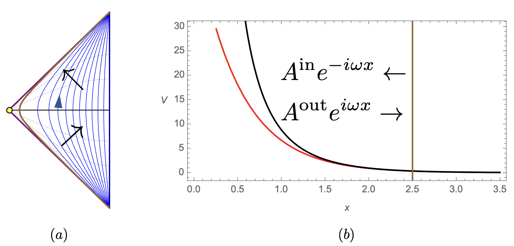
Figure 2: (a) The Penrose diagram for a static patch (b) The scattering potential (36) (black) for a scalar with $\Delta=1.5+0.1i$ and $l=3$ on a static patch in on $dS_{4}$ , which is hardly distinguishable from the Rindler potential (red) in (44) for $x\gg 0$. All quantities are in units of the dS length $\ell_{\text{dS}}$ or its inverse. The horizon is at $x=\infty$. In these diagrams, we indicate the incoming and outgoing waves (37) with black arrows. The brown lines indicate the brick wall regulator [40] at $x=R=2.5\ell_{\text{dS}}$, corresponding to $r\approx 0.987\ell_{\text{dS}}$.

Concretely, the solution to (35) that is regular at $x=0$ is a mixture of plane waves near horizon

$$\psi_{l}(x\to\infty)\sim A_{l}^{\text{out}}(\omega)\,e^{i\omega x}+A_{l}^{\text{in}}(\omega)\,e^{-i\omega x}\;.$$ (37)

Here for real $\omega$ the incoming and outgoing coefficients

$$A_{l}^{\text{out}}(\omega)=\left(A_{l}^{\text{in}}(\omega)\right)^{*}=\frac{\Gamma\left(i\ell_{\text{dS}}\omega\right)}{\Gamma\left(\frac{\Delta+l+i\ell_{\text{dS}}\omega}{2}\right)\Gamma\left(\frac{\bar{\Delta}+l+i\ell_{\text{dS}}\omega}{2}\right)}$$ (38)

are complex conjugates to each other and thus the ratio $\mathcal{S}_{l}(\omega)\equiv A_{l}^{\text{out}}(\omega)/A_{l}^{\text{in}}(\omega)$ is a pure phase. In fact, from (38) we see that $\mathcal{S}_{l}(\omega)$ is a product of two phases:

$$\mathcal{S}_{l}(\omega)=\mathcal{S}^{\text{dS}}_{l}(\omega)\mathcal{S}^{\text{Rindler}}(\omega)$$ (39)

where

$$\mathcal{S}_{l}^{\text{dS}}(\omega)\equiv\frac{\Gamma\left(\frac{\Delta+l-i\ell_{\text{dS}}\omega}{2}\right)\Gamma\left(\frac{\bar{\Delta}+l-i\ell_{\text{dS}}\omega}{2}\right)}{\Gamma\left(\frac{\Delta+l+i\ell_{\text{dS}}\omega}{2}\right)\Gamma\left(\frac{\bar{\Delta}+l+i\ell_{\text{dS}}\omega}{2}\right)}$$ (40)

has the QNM frequencies (30) as poles and their complex conjugates as zeros. In other words, QNMs are scattering resonances associated with the scattering problem (35). The other phase

$$\mathcal{S}^{\text{Rindler}}(\omega)=\frac{\Gamma\left(i\ell_{\text{dS}}\omega\right)}{\Gamma\left(-i\ell_{\text{dS}}\omega\right)}$$ (41)

is $l$-independent and captures all the Matsubara frequencies

$$\omega=\omega_{\pm,n}=\pm i\frac{n}{\ell_{\text{dS}}}\;,\qquad n=1,2,3,\cdots\;,$$ (42)

as its poles and zeros.

The near-horizon Rindler-like scattering problem

The superscript “Rindler” in (41) means that it is actually the scattering phase one would obtain by studying the scattering problem for the same free scalar but on the Rindler-like wedge

$$ds^{2}=e^{-\frac{2}{\ell_{\text{dS}}}x}\left(-dt^{2}+dx^{2}\right)+\ell_{\text{dS}}^{2}d\Omega_{d-1}^{2}\;,\qquad-\infty<x<\infty\;.$$ (43)

The Rindler horizon corresponds to $x=\infty$ while spatial infinity corresponds to $x=-\infty$. The scattering problem analogous to (35) on this wedge is

$$\left(-\partial_{x}^{2}+M_{l}^{2}e^{-\frac{2}{\ell_{\text{dS}}}x}\right)\psi(x)=\omega^{2}\psi(x)\;,\qquad M_{l}\equiv\sqrt{\frac{l(l+d-2)}{\ell_{\text{dS}}}+m^{2}}\;.$$ (44)

Solving for the normalizable solution that exponentially decays at $x\to\infty$, one finds that the scattering phase is given by (41).

Since the metric (43) is nothing but the near-horizon limit of that the full static patch (1), the full S-matrix (39) can be understood in the following way: it consists of a universal part (41) that captures the near-horizon region, which knows nothing about the static patch geometry (except its temperature) and the scalar; the effect of the non-trivial information about the geometry, scalar mass and angular momentum is to “dress" (41) by an extra non-universal phase (40).

Scattering phases and the spectral density

Putting a brick wall cutoff [40] at some large value $x=R$ and imposing a Dirichlet boundary condition, one can compute a smoothed density of states

$$\rho_{l}^{R}(\omega)=\frac{R+\theta^{\prime}_{l}(\omega)}{\pi}+O\left(\frac{1}{R}\right)\;,\qquad\mathcal{S}_{l}(\omega)\equiv e^{2i\theta_{l}(\omega)}\;,$$ (45)

whose divergence as $R\to\infty$ is the origin of the ill-definedness of the trace in (7). However, if we compare our original problem (35) with some reference problem, their difference in DOS is finite as $R\to\infty$:

$$\Delta\rho_{l}(\omega)\equiv\rho_{l}(\omega)-\bar{\rho}_{l}(\omega)=\frac{1}{2\pi i}\partial_{\omega}\log\frac{\mathcal{S}_{l}(\omega)}{\bar{\mathcal{S}}_{l}(\omega)}$$ (46)

where $\bar{\rho}_{l}(\omega)$ and $\bar{\mathcal{S}}_{l}(\omega)$ are the DOS and S-matrix for the reference system. The relation (46) suggests that as opposed to the free energy (9) itself, differences in free energies are well-defined (up to the usual UV-divergence coming from integrating over all energies):

$$\log Z_{\text{bulk}}-\log\bar{Z}_{\text{bulk}}=-\int_{0}^{\infty}d\omega\,\Delta\rho(\omega)\log\left(e^{\beta_{\text{dS}}\omega/2}-e^{-\beta_{\text{dS}}\omega/2}\right)\;.$$ (47)

A priori, there is no unique choice for the reference system. For instance, we can choose it to be the one with zero potential (i.e. an empty box with size $R$), in which case the smoothed density $\bar{\rho}_{l}^{R}(\omega)=\frac{R}{\pi}$ is uniform and has a constant scattering phase.

Uniquely fixing a reference system requires an extra physical input. In the current case, such an input is provided by demanding (47) to equal the Euclidean path integral (6). As it turns out, such a requirement fixes the reference system to be the scattering problem on the Rindler-like wedge (44), i.e. we choose $\bar{\mathcal{S}}_{l}$ to be (41). With this choice,

$$\Delta\rho^{\text{dS}}_{l}(\omega)=\frac{1}{2\pi i}\partial_{\omega}\log\mathcal{S}_{l}^{\text{dS}}(\omega)\quad\;.$$ (48)

Summing over $l\geq 0$, one then recovers the character-regularized DOS (31):

$$\Delta\rho^{\text{dS}}(\omega)=\sum_{l=0}^{\infty}D_{l}^{d}\Delta\rho^{\text{dS}}_{l}(\omega)=\int_{0}^{\infty}\frac{dt}{2\pi}\left(e^{i\omega t}+e^{-i\omega t}\right)\chi_{[\Delta,s=0]}(t)=\tilde{\rho}_{[\Delta,s=0]}(\omega)\;.$$ (49)

Therefore, these considerations imply that the quasicanonical partition function (32) (and therefore by (33) the Euclidean path integral (6)) should be more accurately thought of as a ratio

$$\widetilde{Z}_{\text{bulk}}\equiv\frac{Z_{\text{bulk}}}{Z^{\text{Rindler}}_{\text{bulk}}}\;,$$ (50)

where $Z_{\text{bulk}}\equiv\text{``Tr"}\,e^{-\beta_{\text{dS}}\hat{H}}$ and $Z^{\text{Rindler}}_{\text{bulk}}\equiv\text{``Tr"}\,e^{-\beta_{\text{dS}}\hat{H}_{\text{Rindler}}}$ are the formally defined canonical partition functions for the scalar on the static patch and the Rindler-like wedge (43) respectively, at the dS temperature $T_{\text{dS}}$.

5 1-loop partition functions for spinning fields

In this section we discuss some of the qualitatively new features that arise as one extends our previous discussions to spinning fields. We will set the dS length (or sphere radius) $\ell_{\text{dS}}$ to 1.

5.1 Spinning fields on $S^{d+1}$

We first highlight the subtleties for their 1-loop path integrals on $S^{d+1}$, which have been studied in detail in [14].

5.1.1 Massive fields

Let us start by looking at the example of a free massive vector, whose sphere path integral is

$$Z^{(s=1,m^{2})}_{\text{PI}}=\int\mathcal{D}A\,e^{-S[A]}\;,\qquad S[A]=\int_{S^{d+1}}\left(\frac{1}{4}F_{\mu\nu}F^{\mu\nu}+\frac{m^{2}}{2}A_{\mu}A^{\mu}\right)\;.$$ (51)

Here $S[A]$ is the Proca action. To proceed, one decomposes the vector $A$ into transverse and longitudinal components [41, 42, 43]

$$A_{\mu}=A^{T}_{\mu}+\partial_{\mu}\phi\;,\qquad\nabla^{\mu}A^{T}_{\mu}=0\;.$$ (52)

Here is a subtlety that arises on any compact space: to ensure this decomposition to be unique, one must exclude the normalizable constant mode of the longitudinal scalar $\phi$. In other words, the path integration measure changes as

$$\mathcal{D}A=J\mathcal{D}A^{T}\mathcal{D}^{\prime}\phi\;,$$ (53)

where the prime denotes the omission of the constant mode, and $J$ is the Jacobian associated with the change of field variables $A\to\{A^{T},\phi\}$. One then substitutes (52), (53) into (51) and finds

$$Z^{(s=1,m^{2})}_{\text{PI}}=\det(-\nabla_{(1)}^{2}+m^{2}+d)^{-1/2}(m^{2})^{1/2}\;.$$ (54)

Here the functional determinant is familiar and comes from the integration over $A^{T}$ and $\nabla_{(1)}^{2}$ is the Laplacian acting on transverse vector fields. The factor $(m^{2})^{1/2}$, on the other hand, is only present for Euclidean path integrals on a compact space (in contrast to say $EAdS$), and arises from integrating over $\phi$ while keeping track of the omitted constant mode.

This remains true for general spinning fields: the path integrations over their longitudinal components will lead to a finite number of factors analogous to the factor $(m^{2})^{1/2}$. Such contributions must be present in order to be consistent with locality.

5.1.2 Massless gauge fields

Due to gauge invariance, the path integrals are more intricate for massless gauge fields.

The residual group volume

Let us start with the example of a $U(1)$ gauge field, with path integral

$$Z^{U(1)}_{\text{PI}}=\frac{1}{\text{Vol}(\mathcal{G})}\int\mathcal{D}A\,e^{-S[A]}\,\,,\qquad\text{Vol}(\mathcal{G})=\int\mathcal{D}\alpha=\prod_{n}\frac{d\alpha_{n}}{\sqrt{2\pi}}\;.$$ (55)

The Maxwell action $S[A]=\int_{S^{d+1}}\frac{1}{4}F_{\mu\nu}F^{\mu\nu}$ is invariant under the gauge transformations

$$A_{\mu}\to A_{\mu}+\partial_{\mu}\phi\;.$$ (56)

The volume $\text{Vol}(\mathcal{G})$ of the space of gauge transformations is a path integration over a scalar field $\alpha$, the division by which in (55) compensates for the over-counting of gauge-equivalent orbits related by (56). Proceeding by doing the geometric decomposition (52), $\text{Vol}(\mathcal{G})$ would cancel against the integration $\int\mathcal{D}^{\prime}\phi$ over the longitudinal scalar $\phi$. However, as pointed out in [44], as opposed to $\int\mathcal{D}^{\prime}\phi$, in $\text{Vol}(\mathcal{G})$ we do not exclude the constant mode $\alpha_{0}$ for consistency with locality and unitarity. This implies that the cancellation between $\text{Vol}(\mathcal{G})$ and $\int\mathcal{D}^{\prime}\phi$ is over-complete, leaving a residual factor

$$\text{Vol}(U(1))_{\text{PI}}=\int\frac{d\alpha_{0}}{\sqrt{2\pi}}\;.$$ (57)

If we take into account the possible interactions of the Maxwell field $A_{\mu}$ with other matter fields, the mode $\alpha_{0}$ generates global $U(1)$ symmetries on the matter fields. (57) is therefore the volume of the global $U(1)$ symmetry group. Taking this into account, one eventually arrives at

$$Z^{U(1)}_{\text{PI}}=Z_{\text{G}}Z_{\text{Char}}\;.$$ (58)

The factor

$$Z_{\text{Char}}=\left(d(d-2)\right)^{\frac{1}{2}}\left(\frac{\det^{\prime}(-\nabla_{(0)}^{2})}{\det(-\nabla_{(1)}^{2}+d)}\right)^{\frac{1}{2}}$$ (59)

contains a ratio of determinants, where the denominator is the massless limit of the massive determinant (54); the numerator accounts for the quotient by the pure gauge modes, with the prime denotes the omission of the constant scalar mode. The subscript “Char” means that this part can be written in terms of the $SO(1,d+1)$ characters, which we will come back to in the next section.

The other factor

$$Z_{\text{G}}=\frac{1}{\text{Vol}(U(1))_{\text{can}}}\frac{\mathrm{g}}{\sqrt{(d-2)\text{Vol}(S^{d-1})}}$$ (60)

is essentially (57) modulo the numerical factors $\left(d(d-2)\right)^{\frac{1}{2}}$ in (59). The dependence on the gauge coupling constant $\mathrm{g}$ comes from re-expressing the volume (57)in terms of the volume $\text{Vol}(U(1))_{\text{c}}$ measured with respect to a “canonical metric" which normalizes the $U(1)$ generator to unity.

Conformal factor problem and the Polchinski’s phase

Another example is linearized Einstein gravity on $S^{d+1}$, which has a long and dramatic history [45, 46, 47, 48, 49, 50, 51, 52, 53, 54]. A careful analysis brings the path integral into the form [14]

$$Z_{\text{PI}}=i^{-d-3}Z_{\text{G}}Z_{\text{Char}}\;.$$ (61)

The factors $Z_{\text{Char}}$ and $Z_{\text{G}}$ are analogous to the $U(1)$ case. Specifically,

$$Z_{\text{Char}}= \bigg{(}d(d+2)\bigg{)}^{\frac{(d+1)(d+2)}{4}}\frac{(d-1)^{\frac{d+2}{2}}}{(2d)^{1/2}}\frac{\det^{\prime}(-\nabla_{(1)}^{2}-d)^{1/2}}{\det(-\nabla_{(2)}^{2}+2)^{1/2}}$$ (62)

contains a ratio of determinants capturing the gravition fluctuations and the division by linearlized diffeomorphisms, while

$$Z_{G}=\frac{\gamma^{\frac{(d+1)(d+2)}{2}}}{\text{Vol}(SO(d+2))_{\text{c}}}\;,\qquad\gamma=\sqrt{\frac{8\pi G_{N}}{\text{Vol}(S^{d-1})}}$$ (63)

comes from integrating over the Killing vector modes generating the $SO(d+2)$ isometries. In particular, $Z_{G}$ depends on the Newton constant $G_{N}$ and the canonical isometry group volume $\text{Vol}(SO(d+2))_{\text{c}}$. Note that this is the origin for the logarithmic term in the quantum de Sitter entropy (4).

Compared to the $U(1)$ case, there is a new contribution $i^{-d-3}$ in the path integral (61). To understand the origin of this factor, we note that in manipulating the path integral, we decompose the spin-2 field $h_{\mu\nu}$ into

$$h_{\mu\nu}=h_{\mu\nu}^{\text{TT}}+\frac{1}{\sqrt{2}}(\nabla_{\mu}\xi_{\nu}+\nabla_{\nu}\xi_{\mu})+\frac{g_{\mu\nu}}{\sqrt{d+1}}\tilde{h}$$ (64)

where $h_{\mu\nu}^{\text{TT}}$ is the transverse-traceless part of $h_{\mu\nu}$ satisfying $\nabla^{\lambda}h_{\lambda\mu}=0=h\indices{{}^{\lambda}_{\lambda}}$, $\xi_{\mu}$ the pure gauge part of $h_{\mu\nu}$, and $\tilde{h}$ the trace of $h_{\mu\nu}$. For (64) to be unique, we require $\xi_{\nu}$ to be orthogonal to all Killing vectors and $\tilde{h}$ to be orthogonal to all conformal Killing vectors on $S^{d+1}$ . Now, further expanding these components in terms of spherical harmonics on $S^{d+1}$, one finds that all but a finite number of modes in the trace part $\tilde{h}$ have a negative kinetic term [55]. A standard procedure [55] to cure this “conformal factor problem" is to Wick-rotate $\tilde{h}\to i\tilde{h}$ so that the path integral is well-defined. However, since a finite number of modes have a positive kinetic term to begin with, we must Wick-rotate them back, which eventually leads to this overall phase $i^{-d-3}$ first derived by Polchinski [54]. As shown in [14], an analogous factor is present for any (partially) massless gauge fields with spin $s\geq 2$.

5.2 The edge partition function

Finally, let us make a connection with the Lorentzian/canonical picture discussed in Section 4.2 and 4.3. To start with, one can still define a quasicanonical partition function $\widetilde{Z}_{\text{bulk}}$ by replacing in (32) the character with its spinning counterpart. $\widetilde{Z}_{\text{bulk}}$ still has an interpretation (50) as a ratio between the static patch and Rindler-like canonical partition functions. However, it turns out $\widetilde{Z}_{\text{bulk}}$ is not equal to the Euclidean path integral $Z_{\text{PI}}$. Instead, $Z_{\text{PI}}$ receives some “edge" contributions.

For example, the 1-loop path integral for a massive spin-$s$ field takes the form

$$\log Z_{\rm PI}=\log\widetilde{Z}_{\rm bulk}-\log Z_{\rm edge}=\int_{0}^{\infty}\frac{dt}{2t}\,\frac{1+e^{-t}}{1-e^{-t}}\left(\chi_{\rm bulk}(t)-\chi_{\rm edge}(t)\right)\;.$$ (65)

Here $\widetilde{Z}_{\rm bulk}$ is the quasicanonical partition function (32) and we recall that the massive spin-$s$ character is given by (25). In $Z_{\rm edge}$, the edge character is explicitly given by

$$\chi_{\rm edge}(t)=D_{s-1}^{d+2}\,\frac{e^{-(\Delta-1)t}+e^{-(\bar{\Delta}-1)t}}{(1-e^{-t})^{d-2}}\;.$$ (66)

The case of massless gauge fields works similarly, except that there is an extra contribution from the global group volume factor (and the Polchinski’s phase for spin $s\geq 2$). For instance, the $U(1)$ path integral takes the form $\log Z_{\rm PI}=\log Z_{\text{G}}+\log Z_{\text{Char}}$, where $Z_{\text{G}}$ is given by (60) and

$$\log Z_{\text{Char}}= \log\widetilde{Z}_{\rm bulk}-\log Z_{\rm edge}=\int_{0}^{\infty}\frac{dt}{2t}\,\frac{1+e^{-t}}{1-e^{-t}}\left(\chi_{\rm bulk}(t)-\chi_{\rm edge}(t)\right)$$ (67)

with bulk character (27) and edge character

$$\chi_{\rm edge}(t)=1+e^{-(d-2)t}-\frac{1}{(1-e^{-t})^{d-2}}\;.$$ (68)

Comparing (66) with (25), or (68) with (27), we see that the edge characters live in two lower dimensions than their bulk counterparts. In other words, $Z_{\rm edge}$ is a path integral on a co-dimension-2 sphere, i.e. $S^{d-1}$. This suggests that these describe degrees of freedom living on the bifurcation surface of the dS horizon.

6 Outlook

While the search for a microscopic model for the dS horizon is far from complete, it could be informative to take a closer examination of the low-energy effective field theory. In this note, we have discussed the 1-loop Euclidean path integrals around the round sphere saddle, envisioning the prospect of constraining microscopic models. Conceptually, we have clarified their Lorentzian/canonical interpretation (at least for scalars), all thanks to the powerful tools from $SO(1,d+1)$ representation theory. We would like to conclude with commenting on two intriguing future directions.

Algebra of observables

The canonical partition function (7) can be viewed as the normalization of the reduced density matrix obtained by tracing out the global Bunch-Davis state along the antipodal static patch. This assumes that the global Hilbert space factorizes. From an algebraic QFT viewpoint (reviewed in [57] and discussed in the context of static patch in [58]), such a factorization does not really exist; the algebra of observables for a QFT in a static patch is a Type III von Neumann algebra, which does not admit a trace. The infinity of the single-particle DOS $\rho(\omega)$ in (10) is a manifestation of this non-existence of the trace and thus non-factorization of the global Hilbert space. It is then curious that a version of a trace and therefore quasicanonical free energy (32) can be defined using the $SO(1,d+1)$ Harish-Chandra character. Of course, this does not contradict the considerations in the previous paragraph: as discussed in Section 4.3, (32) is not really a free energy but instead a “renormalized" one. In any case, it would be very interesting to further understand the results presented in this article in terms of algebra of observables associated with a static patch.

Edge modes

In section 5, we discussed a bulk-edge split for spinning path integrals, which certainly resonates with studies of entanglement entropy in gauge theories and gravity. In the early work [59], Kabat found a “contact term” in the conical entropy for Maxwell theory on black holes, which sparked an extensive investigation (see [60, 61, 62, 63, 64, 65, 66, 67, 68, 69, 70, 71, 72, 73, 74, 75, 76, 77, 78] for a partial list) into the proper interpretation for such a contribution as coming from “edge” degrees of freedom living on the the bifurcation surface $S^{d-1}$. In our case of $S^{d+1}$ path integrals, while the physical meaning for the bulk part $Z_{\rm bulk}$ is clear, that for the edge part $Z_{\rm edge}$ is obscure at this point. With the inspirations from these past works, one might be able to clarify the canonical picture for $Z_{\rm edge}$, and it would be very interesting to do so.

References

- [1] G. W. Gibbons and S. W. Hawking, “Cosmological event horizons, thermodynamics, and particle creation,” Phys. Rev. D 15 (May, 1977) 2738–2751. https://link.aps.org/doi/10.1103/PhysRevD.15.2738.
- [2] S. Banerjee, R. K. Gupta, and A. Sen, “Logarithmic Corrections to Extremal Black Hole Entropy from Quantum Entropy Function,” JHEP 03 (2011) 147, arXiv:1005.3044 [hep-th].
- [3] S. Banerjee, R. K. Gupta, I. Mandal, and A. Sen, “Logarithmic Corrections to N=4 and N=8 Black Hole Entropy: A One Loop Test of Quantum Gravity,” JHEP 11 (2011) 143, arXiv:1106.0080 [hep-th].
- [4] A. Sen, “Logarithmic Corrections to Schwarzschild and Other Non-extremal Black Hole Entropy in Different Dimensions,” JHEP 04 (2013) 156, arXiv:1205.0971 [hep-th].
- [5] A. Sen, “Logarithmic Corrections to N=2 Black Hole Entropy: An Infrared Window into the Microstates,” Gen. Rel. Grav. 44 no. 5, (2012) 1207–1266, arXiv:1108.3842 [hep-th].
- [6] A. Sen, “Microscopic and Macroscopic Entropy of Extremal Black Holes in String Theory,” Gen. Rel. Grav. 46 (2014) 1711, arXiv:1402.0109 [hep-th].
- [7] S. Giombi and I. R. Klebanov, “One Loop Tests of Higher Spin AdS/CFT,” JHEP 12 (2013) 068, arXiv:1308.2337 [hep-th].
- [8] S. Giombi, I. R. Klebanov, and B. R. Safdi, “Higher Spin AdSd+1/CFTd at One Loop,” Phys. Rev. D 89 no. 8, (2014) 084004, arXiv:1401.0825 [hep-th].
- [9] S. Giombi, I. R. Klebanov, and Z. M. Tan, “The ABC of Higher-Spin AdS/CFT,” Universe 4 no. 1, (2018) 18, arXiv:1608.07611 [hep-th].
- [10] M. Günaydin, E. D. Skvortsov, and T. Tran, “Exceptional higher-spin theory in AdS6 at one-loop and other tests of duality,” JHEP 11 (2016) 168, arXiv:1608.07582 [hep-th].
- [11] D. Anninos, F. Denef, Y. T. A. Law, and Z. Sun, “Quantum de Sitter horizon entropy from quasicanonical bulk, edge, sphere and topological string partition functions,” JHEP 01 (2022) 088, arXiv:2009.12464 [hep-th].
- [12] V. Shyam, “ + 2 deformed CFT on the stretched dS3 horizon,” JHEP 04 (2022) 052, arXiv:2106.10227 [hep-th].
- [13] E. Coleman, E. A. Mazenc, V. Shyam, E. Silverstein, R. M. Soni, G. Torroba, and S. Yang, “De Sitter microstates from T + 2 and the Hawking-Page transition,” JHEP 07 (2022) 140, arXiv:2110.14670 [hep-th].
- [14] Y. T. A. Law, “A compendium of sphere path integrals,” JHEP 12 (2021) 213, arXiv:2012.06345 [hep-th].
- [15] Y. T. A. Law and K. Parmentier, “Black hole scattering and partition functions,” JHEP 10 (2022) 039, arXiv:2207.07024 [hep-th].
- [16] G. W. Gibbons and S. W. Hawking, “Action integrals and partition functions in quantum gravity,” Phys. Rev. D 15 (May, 1977) 2752–2756. https://link.aps.org/doi/10.1103/PhysRevD.15.2752.
- [17] S. W. Hawking, “Zeta Function Regularization of Path Integrals in Curved Space-Time,” Commun. Math. Phys. 55 (1977) 133.
- [18] D. V. Vassilevich, “Heat kernel expansion: User’s manual,” Phys. Rept. 388 (2003) 279–360, arXiv:hep-th/0306138.
- [19] Z. Sun, “A note on the representations of ,” arXiv:2111.04591 [hep-th].
- [20] A. Higuchi, “Forbidden Mass Range for Spin-2 Field Theory in De Sitter Space-time,” Nucl. Phys. B 282 (1987) 397–436.
- [21] Y. M. Zinoviev, “On massive high spin particles in AdS,” arXiv:hep-th/0108192.
- [22] S. Deser and R. I. Nepomechie, “Anomalous Propagation of Gauge Fields in Conformally Flat Spaces,” Phys. Lett. B 132 (1983) 321–324.
- [23] S. Deser and R. I. Nepomechie, “Gauge invariance versus masslessness in de sitter spaces,” Annals of Physics 154 no. 2, (1984) 396–420. https://www.sciencedirect.com/science/article/pii/0003491684901568.
- [24] L. Brink, R. R. Metsaev, and M. A. Vasiliev, “How massless are massless fields in AdS(d),” Nucl. Phys. B 586 (2000) 183–205, arXiv:hep-th/0005136.
- [25] S. Deser and A. Waldron, “Gauge invariances and phases of massive higher spins in (A)dS,” Phys. Rev. Lett. 87 (2001) 031601, arXiv:hep-th/0102166.
- [26] S. Deser and A. Waldron, “Partial masslessness of higher spins in (A)dS,” Nucl. Phys. B 607 (2001) 577–604, arXiv:hep-th/0103198.
- [27] S. Deser and A. Waldron, “Stability of massive cosmological gravitons,” Phys. Lett. B 508 (2001) 347–353, arXiv:hep-th/0103255.
- [28] S. Deser and A. Waldron, “Null propagation of partially massless higher spins in (A)dS and cosmological constant speculations,” Phys. Lett. B 513 (2001) 137–141, arXiv:hep-th/0105181.
- [29] E. D. Skvortsov and M. A. Vasiliev, “Geometric formulation for partially massless fields,” Nucl. Phys. B 756 (2006) 117–147, arXiv:hep-th/0601095.
- [30] K. Hinterbichler and A. Joyce, “Manifest Duality for Partially Massless Higher Spins,” JHEP 09 (2016) 141, arXiv:1608.04385 [hep-th].
- [31] T. Basile, X. Bekaert, and N. Boulanger, “Mixed-symmetry fields in de Sitter space: a group theoretical glance,” JHEP 05 (2017) 081, arXiv:1612.08166 [hep-th].
- [32] J. Bonifacio, K. Hinterbichler, A. Joyce, and R. A. Rosen, “Shift Symmetries in (Anti) de Sitter Space,” JHEP 02 (2019) 178, arXiv:1812.08167 [hep-th].
- [33] P. R. Brady, C. M. Chambers, W. G. Laarakkers, and E. Poisson, “Radiative falloff in Schwarzschild-de Sitter space-time,” Phys. Rev. D 60 (1999) 064003, arXiv:gr-qc/9902010.
- [34] A. Lopez-Ortega, “Quasinormal modes of D-dimensional de Sitter spacetime,” Gen. Rel. Grav. 38 (2006) 1565–1591, arXiv:gr-qc/0605027.
- [35] A. Lopez-Ortega, “On the quasinormal modes of the de Sitter spacetime,” Gen. Rel. Grav. 44 (2012) 2387–2400, arXiv:1207.6791 [gr-qc].
- [36] Z. Sun, “Higher spin de Sitter quasinormal modes,” arXiv:2010.09684 [hep-th].
- [37] G. S. Ng and A. Strominger, “State/Operator Correspondence in Higher-Spin dS/CFT,” Class. Quant. Grav. 30 (2013) 104002, arXiv:1204.1057 [hep-th].
- [38] D. L. Jafferis, A. Lupsasca, V. Lysov, G. S. Ng, and A. Strominger, “Quasinormal quantization in de Sitter spacetime,” JHEP 01 (2015) 004, arXiv:1305.5523 [hep-th].
- [39] M. R. Tanhayi, “Quasinormal modes in de Sitter space: Plane wave method,” Phys. Rev. D 90 no. 6, (2014) 064010, arXiv:1402.2893 [gr-qc].
- [40] G. ’t Hooft, “On the Quantum Structure of a Black Hole,” Nucl. Phys. B 256 (1985) 727–745.
- [41] O. Babelon and C. M. Viallet, “The Geometrical Interpretation of the Faddeev-Popov Determinant,” Phys. Lett. B 85 (1979) 246–248.
- [42] P. O. Mazur and E. Mottola, “The Gravitational Measure, Solution of the Conformal Factor Problem and Stability of the Ground State of Quantum Gravity,” Nucl. Phys. B 341 (1990) 187–212.
- [43] Z. Bern, E. Mottola, and S. K. Blau, “General covariance of the path integral for quantum gravity,” Phys. Rev. D 43 (1991) 1212–1222.
- [44] W. Donnelly and A. C. Wall, “Unitarity of Maxwell theory on curved spacetimes in the covariant formalism,” Phys. Rev. D 87 no. 12, (2013) 125033, arXiv:1303.1885 [hep-th].
- [45] G. W. Gibbons and M. J. Perry, “Quantizing Gravitational Instantons,” Nucl. Phys. B 146 (1978) 90–108.
- [46] S. M. Christensen and M. J. Duff, “Quantizing Gravity with a Cosmological Constant,” Nucl. Phys. B 170 (1980) 480–506.
- [47] E. S. Fradkin and A. A. Tseytlin, “One Loop Effective Potential in Gauged O(4) Supergravity,” Nucl. Phys. B 234 (1984) 472.
- [48] B. Allen, “Phase Transitions in de Sitter Space,” Nucl. Phys. B 226 (1983) 228–252.
- [49] T. R. Taylor and G. Veneziano, “Quantum Gravity at Large Distances and the Cosmological Constant,” Nucl. Phys. B 345 (1990) 210–230.
- [50] P. A. Griffin and D. A. Kosower, “Curved spacetime one-loop gravity in a physical gauge,” Physics Letters B 233 no. 3, (1989) 295–300. https://www.sciencedirect.com/science/article/pii/0370269389913130.
- [51] P. O. Mazur and E. Mottola, “ABSENCE OF PHASE IN THE SUM OVER SPHERES,”.
- [52] D. V. Vassilevich, “One loop quantum gravity on de Sitter space,” Int. J. Mod. Phys. A 8 (1993) 1637–1652.
- [53] M. S. Volkov and A. Wipf, “Black hole pair creation in de Sitter space: A Complete one loop analysis,” Nucl. Phys. B 582 (2000) 313–362, arXiv:hep-th/0003081.
- [54] J. Polchinski, “The Phase of the Sum Over Spheres,” Phys. Lett. B 219 (1989) 251–257.
- [55] G. W. Gibbons, S. W. Hawking, and M. J. Perry, “Path Integrals and the Indefiniteness of the Gravitational Action,” Nucl. Phys. B 138 (1978) 141–150.
- [56] M. Grewal, Y. T. A. Law, and K. Parmentier, “Black Hole Horizon Edge Partition Functions,” arXiv:2211.16644 [hep-th].
- [57] E. Witten, “APS Medal for Exceptional Achievement in Research: Invited article on entanglement properties of quantum field theory,” Rev. Mod. Phys. 90 no. 4, (2018) 045003, arXiv:1803.04993 [hep-th].
- [58] V. Chandrasekaran, R. Longo, G. Penington, and E. Witten, “An Algebra of Observables for de Sitter Space,” arXiv:2206.10780 [hep-th].
- [59] D. N. Kabat, “Black hole entropy and entropy of entanglement,” Nucl. Phys. B 453 (1995) 281–299, arXiv:hep-th/9503016.
- [60] S. N. Solodukhin, “Entanglement entropy of black holes,” Living Rev. Rel. 14 (2011) 8, arXiv:1104.3712 [hep-th].
- [61] A. R. Zhitnitsky, “Entropy, Contact Interaction with Horizon and Dark Energy,” Phys. Rev. D 84 (2011) 124008, arXiv:1105.6088 [hep-th].
- [62] W. Donnelly, “Decomposition of entanglement entropy in lattice gauge theory,” Phys. Rev. D 85 (2012) 085004, arXiv:1109.0036 [hep-th].
- [63] S. N. Solodukhin, “Remarks on effective action and entanglement entropy of Maxwell field in generic gauge,” JHEP 12 (2012) 036, arXiv:1209.2677 [hep-th].
- [64] W. Donnelly and A. C. Wall, “Do gauge fields really contribute negatively to black hole entropy?,” Phys. Rev. D 86 (2012) 064042, arXiv:1206.5831 [hep-th].
- [65] H. Casini, M. Huerta, and J. A. Rosabal, “Remarks on entanglement entropy for gauge fields,” Phys. Rev. D 89 no. 8, (2014) 085012, arXiv:1312.1183 [hep-th].
- [66] W. Donnelly and A. C. Wall, “Entanglement entropy of electromagnetic edge modes,” Phys. Rev. Lett. 114 no. 11, (2015) 111603, arXiv:1412.1895 [hep-th].
- [67] K.-W. Huang, “Central Charge and Entangled Gauge Fields,” Phys. Rev. D 92 no. 2, (2015) 025010, arXiv:1412.2730 [hep-th].
- [68] W. Donnelly and A. C. Wall, “Geometric entropy and edge modes of the electromagnetic field,” Phys. Rev. D 94 no. 10, (2016) 104053, arXiv:1506.05792 [hep-th].
- [69] H. Casini and M. Huerta, “Entanglement entropy of a Maxwell field on the sphere,” Phys. Rev. D 93 no. 10, (2016) 105031, arXiv:1512.06182 [hep-th].
- [70] S. Ghosh, R. M. Soni, and S. P. Trivedi, “On The Entanglement Entropy For Gauge Theories,” JHEP 09 (2015) 069, arXiv:1501.02593 [hep-th].
- [71] R. M. Soni and S. P. Trivedi, “Aspects of Entanglement Entropy for Gauge Theories,” JHEP 01 (2016) 136, arXiv:1510.07455 [hep-th].
- [72] R. M. Soni and S. P. Trivedi, “Entanglement entropy in (3 + 1)-d free U(1) gauge theory,” JHEP 02 (2017) 101, arXiv:1608.00353 [hep-th].
- [73] W. Donnelly and L. Freidel, “Local subsystems in gauge theory and gravity,” JHEP 09 (2016) 102, arXiv:1601.04744 [hep-th].
- [74] A. Agarwal, D. Karabali, and V. P. Nair, “Gauge-invariant Variables and Entanglement Entropy,” Phys. Rev. D 96 no. 12, (2017) 125008, arXiv:1701.00014 [hep-th].
- [75] A. Blommaert, T. G. Mertens, H. Verschelde, and V. I. Zakharov, “Edge State Quantization: Vector Fields in Rindler,” JHEP 08 (2018) 196, arXiv:1801.09910 [hep-th].
- [76] A. Blommaert, T. G. Mertens, and H. Verschelde, “Edge dynamics from the path integral — Maxwell and Yang-Mills,” JHEP 11 (2018) 080, arXiv:1804.07585 [hep-th].
- [77] J. Lin and D. Radičević, “Comments on defining entanglement entropy,” Nucl. Phys. B 958 (2020) 115118, arXiv:1808.05939 [hep-th].
- [78] J. R. David and J. Mukherjee, “Entanglement entropy of gravitational edge modes,” JHEP 08 (2022) 065, arXiv:2201.06043 [hep-th].