DLRover: An elastic deep training extension with auto job resource computation

Abstract.

The cloud is still a popular platform for distributed deep learning (DL) training jobs since resource sharing in the cloud can improve resource utilization and reduce overall costs. However, such sharing also brings multiple challenges for DL training jobs, e.g., high-priority jobs could impact, even interrupt, low-priority jobs. Meanwhile, most existing distributed DL training systems require users to configure the resources (i.e., the number of nodes and resources like CPU and memory allocated to each node) of jobs manually before job submission and can not adjust the job’s resources during the runtime. The resource configuration of a job deeply affect this job’s performance (e.g., training throughput, resource utilization, and completion rate). However, this usually leads to poor performance of jobs since users fail to provide optimal resource configuration in most cases. DLRover is a distributed DL framework can auto-configure a DL job’s initial resources and dynamically tune the job’s resources to win the better performance. With elastic capability, DLRover can effectively adjusts the resources of a job when there are performance issues detected or a job fails because of faults or eviction. Evaluations results show DLRover can outperform manual well-tuned resource configurations. Furthermore, in the production Kubernetes cluster of Ant Group, DLRover reduces the medium of job completion time by 31%, and improves the job completion rate by 6%, CPU utilization by 15%, and memory utilization by 20% compared with manual configuration.

PVLDB Reference Format:
PVLDB, 14(1): XXX-XXX, 2020.
doi:XX.XX/XXX.XX

PVLDB Artifact Availability:
The source code, data, and/or other artifacts have been made available at %****␣main.tex␣Line␣50␣****%leave␣empty␣if␣no␣availability␣url␣should␣be␣setURL_TO_YOUR_ARTIFACTS.

1. Introduction

Deep learning (DL) has become a powerful tool and has been widely used in various domains. Many practices show that large models fed with large-scale data can significantly improve learning accuracy. For example, in search, recommendation, and advertisement systems, model developers usually use billions of click-through data to train large models with large embeddings.

To train large models with large-scale data, many distributed DL training frameworks have been developed. Generally, there are asynchronous (e.g., Parameter Servers) and synchronous (e.g., AllReduce) models to train deep learning models. AllReduce approach attracts more attention since it provides the benefits of fast convergence and a stable model compared to asynchronous approaches. Compared to AllReduce, the asynchronous approaches like PS framework work better in the unstable cloud environment since those approaches do not require each node of a job to coordinate in a strictly synchronous way. TensorFlow (Abadi & et al., 2015) or PyTorch with parameter server (Li et al., 2014) is widely used to train DL models in a cloud environment (xxxx), and such kind of deep learning training job contains two kinds of compute nodes: worker and parameter server (PS), respectively. The worker computes gradients with training samples, while the PS stores model parameters and updates parameters using gradients from workers.

There are still a couple of challenges to running a DL job in the cloud efficiently. First, the resources of a job (e.g., the number of workers and PS, each node’s CPU and memory, etc.) play key roles in the performance of the job. However, improper resource configurations have been observed in many training jobs. Since the resource configuration could significantly impact a job’s performance or even fail the job (e.g., OOM), it is critical to run a training job with appropriate resource configuration. Second, resource sharing in the cloud could impact a running job, even interrupt the running job, e.g., one node of the job is evicted by jobs with higher priority. It is extremely inefficient to re-run those jobs from the beginning. Therefore, elasticity and fault tolerance are also necessary to run DL training jobs in the cloud.

According to our observation, most users fail to configure their jobs with appropriate resources. Many users prefer to configure their jobs with over-provisioned resources to avoid any potential risk from insufficient resources. This usually ends up in huge resource waste. Figure 3 illustrates a one-week statistic of CPU and memory utilization of those jobs. As shown in the figure, more than 80% of jobs’ CPU and memory utilization is below 50%. Thus, even with up to 20,000 CPU cores and 200TB RAM resources in the cluster, some new jobs are still pending to create because of insufficient resources since many running jobs are occupying too many unnecessary resources. The pending time is considerably longer for new jobs requiring a large number of resources (CPU cores, etc) to train large-size models, as illustrated in Figure 3. Except for this resource over-provision problem, there is still an under-provision problem observed in about 5% of the jobs. Those jobs usually run into OOM failure with insufficient memory. These two observed problems indicates that it is a common case for users to set inappropriate resources for their jobs.

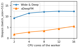
(a) Fixed 1 PS, 16 CPU

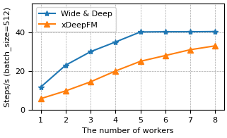
(b) Fixed 1 PS, 16 CPU

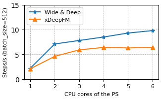
(c) Fixed 1 worker, 16 CPU

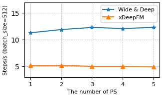
(d) Fixed 1 worker, 16 CPU

Figure 1. The relationship between throughput and resources

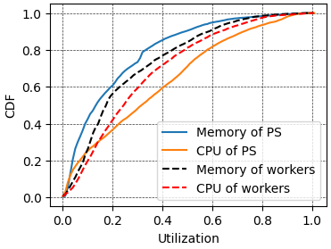
Figure 2. Resource util

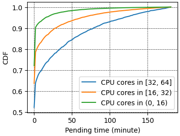
Figure 3. Pending time

A popular approach to configuring jobs’ resources adapted by many users is trial-and-error. Users manually run the same job repeatedly with different resources to search for the optimal resource configuration. However, trial-and-error is very time-consuming since a new job needs to launch Pods, prepare the runtime environment, and initialize the computation graph. Users have to wait for a while before they can observe useful information like the throughput and resource utilization of this job. Meanwhile, the trial-and-error approach wastes too many resources since a job has to be run multiple times before starting the actual model training.

Therefore, there is a strong demand to free users from manual resource configuration, and users can focus on tuning the DL model performance (e.g., precision or recall) instead. Ideally, a training job can be submitted to a k8s cluster without any resource configuration, and there is a system that can provide optimal resource configuration to the job automatically. With such a system, users can evidently avoid job failure and poor performance.

Guided by this insight, we have designed and implemented a new distributed DL system named DLRover for asynchronous training using Parameter Server framework. DLRover can run DL training jobs for the optimal performance (i.e., throughput) through resource auto-configuration and dynamic resource adjustment. More specifically, DLRover keeps monitoring running jobs during their lifetimes and provides optimal resource plans when necessary. With efficient elasticity, DLRover can apply those new resource plans and adjust corresponding jobs’ resources quickly. The main contributions of DLRover are listed below:

• Automatic resource configuration. Initially, DLRover  generates a resource configuration (e.g. the number of nodes, CPU and memory of each node) for one new job based on historical job data. Latterly, DLRover continually collects runtime information (e.g. workload and throughput) of the job and generates new resource plans based on the newly developed optimization approach to improve the job runtime performance. As a result, when a straggler node is observed, DLRover will adjust the resources or workload of the straggler node.

• Elasticity. DLRover has implemented an efficient elasticity framework and can adjust the resources of running jobs quickly. More specifically, DLRoverpropose a new optimization algorithm to reduce the transition time of elasticity (i.e., time to adjust the job’s resources) and support frequent adjustment.

• Fault tolerance. DLRover develop an extension framework to support the fault tolerance during train. Therefore, when there are one or more failed nodes in a job, DLRover can recover failed nodes and resume the training automatically and will not re-run the job from the beginning.

The remainder of this paper is organized as following: Background discusses DL recommendation model and elasticity of TensorFlow. Design gives the overview of DLRover. DLRover Brain introduces how the jobs’ resource plans are generated. Elastic Trainer describes how to provide elasticity to jobs. Evaluation illustrates how DLRover improves the performance and resource efficiency of jobs. Related work compares DLRover with existing works, followed by Conclusion.

2. Preliminary and Motivation

2.1. Deep learning recommendation models

The Deep learning recommendation model (DLRM) jobs are one of the major job types in our cluster. Here we would like to discuss the features of DLRM jobs and how those features affect the elasticity design. We will also discuss the limitation of the elasticity in the existing TensorFlow framework.

DLRM has been widely used for CTR prediction on online E-commerce, advertisement and news feeds. In our cluster, there are thousands of DLRM jobs which are consuming 200TB RAM and 20,000 CPU cores daily. In DLRM, data sparsity is a challenging problem since the number of items is extremely huge. Users usually use item embeddings to represent each item as a dense numeric vector before NN layers (Naumov et al., 2019). In TF training framework, parameters of DLRM are partitioned across PS. When to adjust the PS, it usually stops the training of the job and checkpoint those parameters. After that, a new job with new PS configuration is created from the checkpoint. However, such new job needs to initialize the training process which includes building the computation graph, initializing TF operators and restoring the model from a checkpoint. Due to the large size of embedding data (Figure 4) and the considerable number of PS and workers in a DLRM job, the time cost to start a new job become unacceptable. Therefore, we must find a way to minimize the transition time for elasticity. Otherwise, the benefit of the elasticity could be negative since it delays the completion of the job significantly.

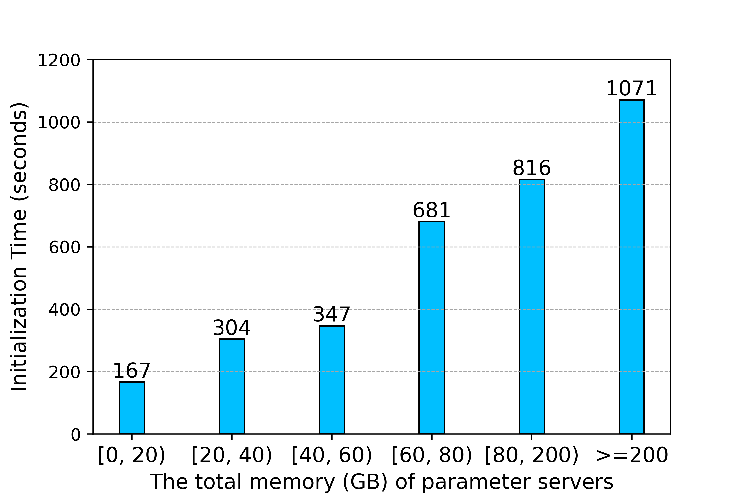
Figure 4. The median initialization time of PS jobs in Ant Group

2.2. Distributed Deep Learning Model Training

Parameter Servers

Ring all-reduce Distributed Training

2.3. Limitations of Existing Training Systems

There is no complete and efficient elasticity solution in existing TensorFlow framework. To be more specific, TF framework does not provide any support to PS elasticity and only limited support to worker elasticity. For worker elasticity, TensorFlow allows new workers to join the training cluster of the job by propagating new cluster specification automatically. The job scheduler can add/remove one or more workers at little cost since each worker is training the model independently. However, that is all provided by the native TensorFlow. In order to have the complete elasticity, users need to implement their own dynamic data partition for the change of workers. A direct solution is to halt training on workers and redistribute dataset according to the new worker group and resume the training. This way will stop all workers’ execution and each repartition can not guarantee balanced workload on each worker and hurts the convergence. A reasonable dynamic partition design is required for efficient worker elasticity.

In general, an appropriate resource configuration requires expert-level experience in distributed deep learning since there are a couple of challenges here. First, different models have quite different resource requirements. As Figure 1 shown, both wide & deep (Cheng et al., 2016) and xDeepFM (Lian et al., 2018) jobs’ throughput improve significantly with more CPU in each PS. However, the xDeepFM (Lian et al., 2018) job has heavier computation than wide & deep and needs more CPU cores ( Figure 1(a) and Figure 1(b)). Second, a job needs to be configured with multiple types of resources. A single type of resource, even with an optimal configuration, has the limitation of improving the job’s performance. For example, the throughput of wide & deep can be improved with more CPU of the worker initially (Figure 1(a)). However, it reaches the limitation when the worker is already allocated with more than 8 CPU cores since PS is the bottleneck now. More CPU in the worker can not improve the job’s performance further.

However, the estimation of a newly created job’s required resource usually is not 100% accurate, and we still need to scale those jobs dynamically during their runtime. First, the cloud environment is complicated and unstable. Usually, DL jobs are co-located with other jobs (e.g., online services) and share the resources of the same machines. In terms of co-location, online services have much higher priority (Jiang et al., 2020) and DL jobs’ performance will be sacrificed when online services demand more resources. Then the PS or workers of the training job may become a straggler, even evicted from the machines. Second, the diversity of models indicates quite different resource requirements during their training process. As Figure 1 shows, xDeepFM jobs are demanding much more CPU resources than wide & deep jobs. Therefore, the inaccurate resource estimation as well as resource sharing in the cloud require an efficient elasticity implementation to fix the inaccuracy in the estimation and handle unpredictable resource-sharing issues.

3. The Overview of DLRover

In this section we introduce the overview of automatic resource optimization and elasticity in DLRover. At first, we describe the design principles behind DLRover. Later we give the architecture of DLRover.

3.1. Design principles

As mentioned in section 1, it is difficult to have the accurate estimation on jobs’ optimal resources considering the diversity of the training models and dynamic cloud environment. Furthermore, any complicated algorithm or model usually requires non-trivial computation to have the resource estimation for a job, which could result in observable delay to users. Thus, instead of relying on the accuracy of estimation algorithms, we tend to develop a system with efficient elasticity support and can adjust the job resources based on its runtime statistics quickly. The design principles of DLRover are listed as follows:

1. With efficient algorithms, DLRover can have the initial resource configuration for a new job and start the job quickly. Then based on the runtime statistics of the job, DLRover keep optimizing this job’s performance through continuously resource adjustment.

2. Both PS and workers can influence the performance of a job. However, the cost of adjusting PS is much higher than adjusting workers in a TensorFlow training job. Thus DLRover is inclined to adjust workers at first and only adjust PS when it is necessary.

3. The transition time is the key to the efficiency of elasticity. We need to minimize the transition time for both PS and workers’ elasticity.

3.2. System architecture

DLRover has three major components: ElasticJob operator, DLRover Brain and Elastic Trainer. ElasticJob operator is used to launch/remove Pods on a k8s cluster. ElasticJob operator contains two kinds of custom resource definition (CRD) of k8s, one is ElasticJob CRD specifing the training program, another is Scale CRD specifying the PS/worker resource configuration. DLRover Brain is a resource optimization service for all training jobs and is deployed as a k8s deployment. For each job, an Elastic Trainer is created to support PS/worker elasticity during the whole life cycle of a job.

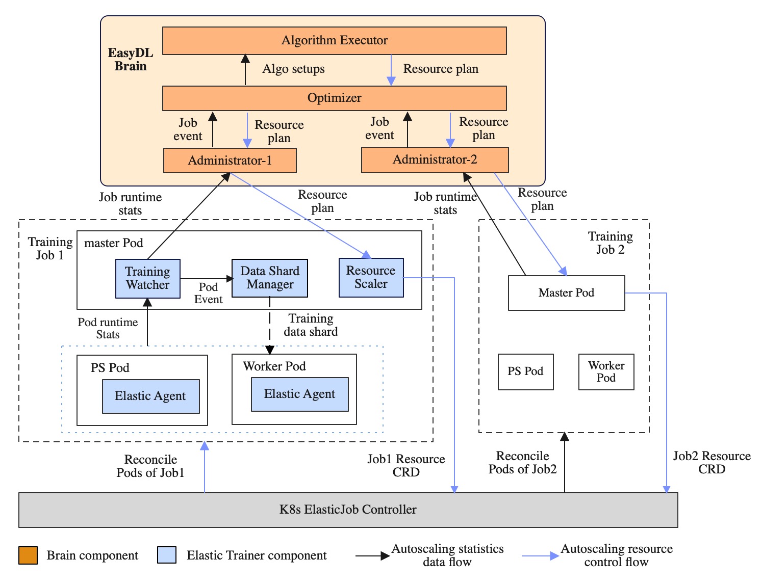
Figure 5. DLRover overview

Figure 5 shows how DLRover manages DL training jobs on a k8s cluster. Users wrap up a training job as an ElasticJob CRD and submit it to the cluster. After receiving the CRD, ElasticJob operator creates a Elastic Trainer for the job by starting a master Pod. Then Elastic Trainer informs DLRover Brain the new job and DLRover Brain will return the initial resource plan to Elastic Trainer. After that, Elastic Trainer creates Scale CRDs from the plan and apply the Scale CRD to notify ElasticJob operator to launch required Pods and each Pod will start a Elastic Agent on it. During training, Elastic Trainer dispatches data shards to workers, keeps collecting runtime statistics (e.g., CPU, memory usage, and training progress) and reports them to DLRover Brain periodically. Based on the job’s running status, DLRover Brain picks up appropriate algorithms to generate new resource plans and informs Elastic Trainer to start resources adjustment.

4. DLRover Brain

DLRover Brain is responsible to generate the initial resource plans for new created jobs. After jobs starts to run, DLRover Brain continuously tracks the performance of the running jobs and generates resource plans when a job has a performance issue. The plan is sent to the corresponding job master and executed by the Elastic Trainer in the master to adjust this job’s resources accordingly.

4.1. Resource-throughput modeling

A complete training process consists of many steps. For each step, the computation workload includes two parts: 1. computing gradients by forward and backward computation with a batch data, donated as $W_{compute}$; and 2. updating parameters on parameter servers with those gradients, donated as $W_{update}$. Since parameters are partitioned across parameter servers and updated independently by each parameter server, $W_{update}$ is shared by those parameter servers. Assuming a job has $N_{ps}$ parameter servers and the $j$th parameter server has $s_{j}$ CPU cores, the total available CPU cores $s_{total}$ for update is $\sum_{j=0}^{N_{ps}}s_{i}$. We assume a single CPU’s computation capacity is $r$. Then we can model the time of a step as below:

$t_{compute}$: the time of a worker to compute gradients. It can be modeled as $\frac{W_{compute}}{r\cdot\min(w_{i},\hat{w})}$. Here $\hat{w}$ is the actually used CPU of the computation and $w_{i}$ is the configured CPU cores of the $i$th worker.
$t_{update}$: the time of parameter servers to update parameters with gradients. Assuming parameters are evenly partitioned across all PS, $t_{update}=\frac{W_{update}}{r\cdot\min(s_{total},\hat{s})}$. $\hat{s}$ is actually used CPU cores in the update of a step.
$t_{IO}$: the time to read and pre-process a batch data from the data store, to transfer parameters and gradients between the worker and parameter server.

With the definition above, we can have the throughput of a single worker with batch size $B$. Then the throughput of a job with $N_{w}$ workers, donate as $R$, is the sum of all workers’ throughput.

(1) $$R=\sum_{i=0}^{N_{w}}\frac{B}{t_{IO}+\frac{W_{compute}}{r\cdot\min(w_{i},\hat{w})}+\frac{W_{update}}{r\cdot\min(s_{total},\hat{s})}}$$

Obviously, $R$ is increasing with larger $N_{w}$, $w$, $s_{total}$. However, those jobs are sharing the resources of a cluster and each job can only enjoy limited resources for the fairness. Here a job can only allocated with a maximum $C_{total}$ CPU cores in total. Meanwhile, $w$ and $s$ also has constraints since a machine can only have $C_{max}$ CPU cores. Furthermore, the performance of a job is affected by both workers and parameter servers. When $N_{w}$ workers push gradients at the same time, the update workload is $N_{w}\cdot W_{update}$ and parameter servers should have $N_{w}\cdot\hat{s}$ CPU cores to process those updates. Otherwise parameter servers are overloaded and the throughput $R$ can not be further improved with more workers. Then we must guarantee parameter servers are not the bottleneck, which is: $N_{w}\cdot\hat{s}<s_{total}$. So, we need to maximum $R$ with constraints as following.

(2) $$\text{maximize}~{}~{}R$$

(3) $$\text{subject to}:\sum_{i=0}^{N_{w}}w_{i}+\sum_{j=0}^{N_{ps}}s_{i}<C_{total}$$

(4) $$N_{w}\cdot\hat{s}<\sum_{j=0}^{N_{ps}}s_{i}$$

(5) $$w_{i}<C_{max},s_{j}<C_{max}$$

(6) $$N_{w}\in Z^{+},N_{ps}\in Z^{+},w_{i}\in Z^{+},s_{j}\in Z^{+}$$

The problem is a non-linear integer programming problem and is NP-hard in general. We assume that workers have the same CPU cores $w$ and parameter servers have the same CPU cores $s$, then $s_{total}=N_{ps}\cdot s$. We can split the problem into 2 sub-problem: 1. Resolve $w$ and $s_{total}$ to maximize the throughput of a worker. 2. Resolve $N_{w}$, $s_{total}$ to maximize $R$ of a job.

For sub-problem 1, we only need to ensure $w\geq\hat{w}$ and $s_{total}\geq N_{w}\cdot\hat{s}$ if we can get the required CPU cores $\hat{w}$ of the worker and $\hat{s}$ of parameter servers. For a DL model defined by TensorFlow, it is difficult to estimate $\hat{w}$ and $\hat{s}$ without starting the training since TensorFlow pipelines the computation of the model within the same devices and supports parallel execution of a core model dataflow graph with many devices (Abadi & et al., 2015). Thus we launch a couple of parameter servers and only one worker at first to estimate $\hat{w}$ and $\hat{s}$ and assign $w=\hat{w},s=\hat{s}$.

Then, the sub-problem 2 can be solved as below:

(7) $$\text{maximize}~{}~{}N_{w}$$

(8) $$\text{subject to}:N_{w}\cdot\hat{w}+N_{w}\cdot\hat{s}<C_{total}$$

(9) $$N_{w}\in Z^{+},N_{ps}\in Z^{+}$$

We can have:

(10) $$N_{w}=\frac{C_{total}}{\hat{w}+\hat{s}}$$

(11) $$s_{total}=C_{total}-N_{w}\cdot\hat{w}$$

After $s_{total}$ is resolved, we need to resolve $N_{ps}$ and $s$. In TensorFlow, the number of Send and Receive operations added to the graph on the worker are proportional to $N_{ps}$. If we set a small $N_{ps}$, we need to set a big $s=\frac{s_{total}}{N_{ps}}$. However, the pending time of creating a new Pod is positive correlation with CPU cores required by the Pod (Figure 3). In our cluster, we find that $s=16$ is a reasonable value which balance the trade off between $s$ and the pending time.

4.2. Dynamic Job Resource Configuration

In this part, we introduce how we maximize throughput (Equation 2) with the help of the elasticity in DLRover. According to sub-problems in subsection 4.1, we split approaches into two stages: Sampling to maximize the throughput of a worker, optimization to maximize the throughput of a job.

However, we found our algorithms (Equation 2) do not always give the optimal result since the algorithms are based on ideal assumptions. For example, sometimes parameters are not evenly partitioned across all parameter servers. TensorFlow distributes parameters to parameter servers in unit of Tensor (i.e., a typed multidimensional array) and some tensors are possible to have larger size. Then there is unbalanced workload on parameter servers and results in straggler problems. Thus, we add an extra stage named adjust after optimize to fix those problems.

Sampling to estimate required CPU cores. When a new job is submitted, we launch a few parameter servers and a worker with the default CPU cores $C_{max}$ and default memory. If the worker fails with OOM, DLRover launches a new worker with double memory. Similarly, if any PS fails with OOM, DLRover doubles the number of PS that PS can have more total memory to load the model. After the job starts to run, we check the CPU utilization of each worker and PS. Assuming the worker has used $\hat{w}$ CPU cores and the total used CPU cores of all PS are $\hat{s}$. If the CPU utilization of PS exceeds a predefined threshold like 0.9, DLRover will add more CPU cores to PS.

Optimize to compute the optimal resource. At the stage, we firstly scale up the CPU cores of PS to $s_{total}$ by Equation 11. We set $s=16$ and $N_{ps}=\frac{s_{total}}{s}$. The graph of the workers varies with different numbers of PS which results in the change of workload. After the new configuration of the job takes effect, we estimate the $\hat{w}$ again and scale up worker number to $N_{w}=\frac{s_{total}}{\hat{s}}$. Each new worker is allocated with $\hat{w}$ CPU cores and its memory is from the observation on the actual used memory of running workers. Table 1 shows the optimization result and job throughput $R$ of Wide & Deep (W&D) and xDeepFM (xDFM) with $C_{total}=200$. The speed-up ratios of W&D and xDFM are 0.81 and 0.96 which demonstrates our algorithms’ effectiveness.

As Figure 6 shows, parameter distribution of xDeepFM is more even than Wide & Deep and have better speed-up ratio (i.e., 0.96 vs 0.73). This shows that ours algorithms works better when each parameter server has balanced workload.

Adjust to fix performance problems. At this stage, DLRover collects the runtime information of each pod and further adjust resources to fix following problems:

Idle CPU resource in PS. Due to the inaccuracy of the estimation of $\hat{s}$ or worker stragglers, PS could not make full usage of their CPU cores sometimes, e.g., xDeepFM in Figure 6. DLRover recompute $\hat{s}$ by equation $\hat{s}=\frac{\hat{s_{total}}}{N_{w}}$ and add more workers, which is computed by $\Delta N_{w}=\min(\frac{s_{total}}{\hat{s}},\sqrt{K})-N_{w}$.In this way, we can improve the throughput of jobs further. For example, the throughput of the xDeepFM job reaches 56 steps/s after adding more 2 workers. At the moment, the job may already exhausted its CPU quota (i.e., $C_{total}$ in total). However, ElasticJob can still launch new workers for this job. Note those workers are marked as low priority and can be preempted when CPU resources of the cluster are tight. Relaxing the constraint on each job’s total CPU can also improve the overall resource utilization of the cluster.

Hot parameter server. Unbalanced workload usually leads to one or more PS become hot spot (Figure 6). When this happens, DLRover launches a new PS with more CPU cores to replace the hot one. The CPU cores of new PS is computed by $s=\min(\frac{\hat{s_{hot}}}{\hat{s_{total}}}\cdot\hat{s}\cdot N_{w},C_{max})$. Here $\hat{s_{hot}}$ is the current CPU usage of the hot PS and $\hat{s}$ is the CPU usage of all PS where there is one worker. $\frac{\hat{s_{hot}}}{\hat{s_{total}}}\cdot\hat{s}\cdot N_{w}$ is the CPU requirement of $N_{w}$ worker on the hot PS. In the Wide & Deep job, we replace PS-2 and PS-3 with pods with 24 CPU cores, the throughput can increase to 258 steps/s.

model	stage	$N_{w}$	$w$	$N_{ps}$	$\hat{w}$	$\hat{s_{total}}$	$R$
W&D	sample	1	32	1	2.5	5.7	12
	optimize	24	3	8	2.3	85.1	210
xDFM	sample	1	32	1	19.4	3.1	6.2
	optimize	8	20	2	18.3	27.4	47.8

Table 1. Throughput with Optimization Results (The unit of R is step/s, batch size=512)

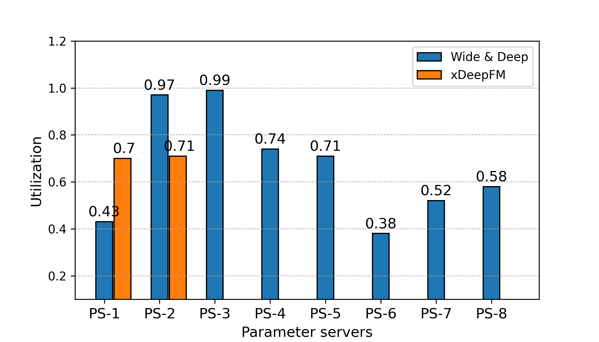
Figure 6. The CPU utilization of PS

4.3. Implementation of DLRover Brain

As mentioned above, we use different algorithms for the best resource plans during different stages of a job. When a job is created, we have no any runtime information (e.g., $\hat{w}$ and $\hat{s}$) of this job and can only rely on static information (e.g., data source and user) and relevant historic data (e.g., information of completed jobs that are using the same table in their training) to generate the initial resource plan. After this job runs for a while, DLRover accumulates enough running status of the job and can have the estimation of $\hat{w}$ and $\hat{s}$. Then DLRover can compute $N_{ps}$ and $s$ when it has the workload of each node (i.e., PS and worker) and the global step. Usually this optimization process starts after the job has finished certain computation, e.g., complete more the 100 global steps or after 60s. After the adjustment, DLRover continually monitors the performance of a running job. When there is a performance issue in the job, DLRover Brain immediately triggers another optimization process which will: 1. determine the root cause of poor performance, e.g., straggler or insufficient CPU cores of nodes; 2. picks up the corresponding algorithm and generate a new resource plan.

We have implemented jobs’ resource optimization including monitoring, analyzing and optimizing in DLRover Brain, rather than making each job to optimize itself due to a couple of concerns. First, the optimization requires to run complicated algorithms which could squeeze too many resources of the master Pod and influence the master Pod’s other tasks. If we allocate more resources to the master Pod for optimization, it could ends up with a waste of resources since the monitoring is only triggered periodically or when there is a performance issue observed. It is more easier to scale up and down an independent service according to the current monitoring workload. Secondly, an independent service allows to iterate new algorithms in a more easy way. If we locate algorithms in each job, it is difficult to update those algorithms once a job starts.

Considering there is a demanding to iterate optimization algorithms frequently, those algorithms are implemented as plugin functions in DLRover Brain. Each optimization can switch between different algorithms easily. The details of our optimization algorithms can be found in subsection 4.2.

DLRover Brain consists of three major components: administrator, optimizer, and algorithm executor.

Administrator tracks each running job and starts a job optimization event when predefined conditions are meet. When a new job is created in the cluster, a corresponding administrator is created for the new job in DLRover Brain. This administrator is monitoring this job during the job’s entire lifetime. The administrator can be implemented to trigger job optimization events periodically or for a predefined event (e.g., the model iteration starts). When the job is completed, the administrator will also stop and removed.

Optimizer is responsible to process the optimization event created by administrators. Different types of events are forwarded to different optimizers for further processing. Based on the runtime information of the job, the optimizer determines the status of this job and picks up the best algorithms to generate new resource plans.

Algorithm Executor receives the request from optimizers and execute required algorithms and generate resource plans. Since those executors are stateless, we can create more executors when there are more running jobs. The number of executors is configured in the configuration file of DLRover (i.e., a configure map in the k8s cluster) and can be updated dynamically.

5. Elastic Trainer

When a new job is created, an Elastic Trainer is also created with the new job to provide elasticity support. Elastic Trainer is responsible for two main tasks: 1. adjusting the job’s resources according to resource plans; 2. providing fault-tolerance to the job. Meanwhile, Elastic Trainer must guarantee consistency between parameters and training dataset at any time. Assuming gradients are computed from training samples and applies to update corresponding parameters on PS, consumed samples should not be used again in this epoch.

5.1. Design of Elastic Trainer

Elastic Trainer consists of a Pod Watcher, a Data Shard Manager and multiple Elastic Agent. Pod Watcher is to watch events of all Pods in the job, collect the workload stats of Pods and report those stats to DLRover Brain. Data Shard Manager is to partition a dataset into shards and manage the feeding of those shards to each worker. It dispatches shards to workers for training and removes completed shards. When a worker is terminated with an uncompleted shard, the manager will dispatch this shard to another worker. To enable Elastic Trainer, users need to use Elastic Agent to query data shards from Data Shard Manager in the data pipeline of training loop.

5.2. Dynamic data sharding

The dataset for a training job usually is split evenly according to the number of workers. The data sharding in native TF framework is static and can not be modified during runtime. However, in light of elasticity, the number of workers can change at any time, hence DLRover should be able to assign data shards to workers dynamically. Meanwhile, the adjustment cost must be minimized since DLRover could adjust the job frequently to approach the optimal resource configuration quickly. Here we have designed and implemented the dynamic data sharding policy in DLRover, to handle the dynamic number of workers.

The training dataset consists of a lot of samples and each sample is marked by an index. Unlike static sharding, Data Shard Manager does not partition the dataset according to the number of workers. Instead, the manager splits the dataset into many much smaller shards. Note a shard does not contain samples directly. Instead, a shard only includes indices of those samples. All shards are placed into a TODO queue. After a worker starts to run, the data input pipeline of a worker will query one shard from Elastic Trainer and read samples by indices in the shard. Meanwhile, Data Shard Manager marks this shard with the id of the worker and moves the shard from the TODO to the DOING queue. After a worker consumes samples in the shard and update the new parameters in PS, it reports to Elastic Trainer and queries a new shard. Then Data Shard Manager deletes the finished shard from the DOING queue.

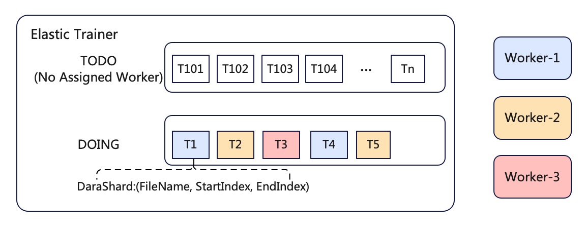
Figure 7. Dynamic Data Sharding

5.3. Elasticity support

Elastic Trainer can provide efficient elasticity support to jobs that can dynamically adjust the number and resources of PS and workers. Meanwhile, Elastic Trainer also provides fault tolerance to jobs and can resume training when there is a node failure in the job.

Worker elasticity. In asynchronous SGD, each PS updates parameters with gradients from a worker independently and does not synchronize with other workers. Thus, Elastic Trainer can add or remove workers without influencing other workers. After a new worker starts, it connects to all PS and queries shards from Data Shard Manager and consume shards to compute gradients. If a worker is terminated, Data Shard Manager moves uncompleted shards of this worker back to the TODO queue from the DOING queue. Later the shard can be dispatched to another workers.

Parameter server elasticity. Unlike workers, PS hold the states (i.e., trainable parameters) of the job and it has to re-partition those parameters when to change the number of the PS. DLRover has implemented an efficient way to achieve PS elasticity through checkpoint. Unlike native checkpoint approach, DLRover does not restart nodes (i.e., workers and PS) and minimizes the waiting period for new PS.

When to add new PS, workers continue to train the model until all new PS are ready. Then the master updates PS information on each worker and halts workers’ execution. After that, the chief worker (i.e., worker with rank 0) checkpoints parameters on all old PS and re-partition parameters according to new PS number. Then each PS restores its part of parameters from the checkpoint. Finally PS and workers join a new training cluster and continue to train the model. Removing PS is similar to adding PS except DLRover only removes PS after the training is resumed in PS and workers. Note workers do not wait for the creation and initialization of new PS which minimizes transition time of PS elasticity. In light of failure, Elastic Trainer can not checkpoint states in advance. Thus, Elastic Trainer periodically checkpoints parameters, TODO and DOING shard queues. When a PS fails, Elastic Trainer can easily restore parameters and shard queues from the latest checkpoint.

5.4. Straggler mitigation

Straggler is a node which is significantly slower than others. If a worker is straggler, Data Shard Manager would dispatch fewer data shards to this worker. With less workload, the worker has a chance to catch up with other workers again. However, for PS stragglers, Elastic Trainer has to carefully determine the root cause at first. If the straggler has higher resource usage than other PS, it is quite possible to have an unbalanced workload on this PS. Elastic Trainer can mitigate the impact by adding more resources to the straggler PS. If not, it is more likely that there are problems with the physical machine. Then Elastic Trainer has to migrate the PS to a new machine.

6. Evaluation

We have implemented DLRover in Python and Go languages as an open-source package on github. Elastic Trainer is implemented in around 20,000 lines of Python codes while DLRover Brain is implemented in around 12,000 lines of Go codes. Elastic Agent of Elastic Trainer are implemented for TensorFlow. DLRover is a native Kubernetes system and can be easily deployed on a Kubernetes cluster.

We have deployed DLRover in the cluster of Ant Group to manage thousands of jobs in search, recommendation, and advertisement. We collect two-week statistics of productive training jobs using DLRover without any resource configuration input from users. We evaluate the performance on the job completion time (JCT), resource utilization, and the job completion rate. Here completion rate is equal to the number of successful jobs over the number of all jobs created. Note that, if a job fails in the middle and users re-run it, this job is marked as fail and the re-run job is counted as a new job.

6.1. Evaluation setup

We compare DLRover with static manual configurations and existing heuristics scaling algorithms mainly on the JCT and resource utilization. We conduct all experiments on a k8s cluster of Ant Group and jobs in the experiment are allocated at most 200 CPU cores. The machines in the cluster are equipped with an Intel Xeon E5-2682 @2.5GHz and 192GB RAM. A single Pod can only be allowed to allocate a maximum of 32 CPU cores. In the experiments, the interval time period between two elasticity of DLRoveris at least 60s.

We use Wide & Deep and xDeepFM with Criteo dataset in experiments. Wide & Deep is IO intensive and xDeepFM is computation intensive. The batch size is 512 and the epoch is 5 for each job. We randomly split the dataset into 90% for training and 10% for testing. We use TFJob framework in KubeFlow (George & Saha, 2022) as comparison to DLRover. Each TFJob job’s resources are configured manually. For TFJob, we evenly split the dataset into shards according to the number of workers.

6.2. Comparison with static well-tuned resources

Here we want to show the result of DLRover is quite close to well-tuned manual configurations for normal jobs (i.e., without stragglers) and DLRover can outperform well-tuned TFJob when there are stragglers.

Normal jobs. We manually tune the job’s resource configuration repeatedly until it almost reaches the best throughput. Table 2 gives the well-tuned resource configuration for Wide & Deep and xDeepFM. The detailed comparison can be found in Table 2. Results support our claim that the performance of DLRover is almost the same as well-tuned configuration. However, a well-tuned configuration requires non-trivial efforts and expert-level knowledge in distributed TF training, which is impractical approach for many users.

Jobs with stragglers. To simulate the worker and PS straggler, we randomly select a worker or PS and set the CPU cores to 25% of the CPU cores in Table 2. Figure 8 gives the comparison between DLRover and well-tuned configurations. For worker straggler case, DLRover can shorten JCT by 24% for Wide & Deep and 42% for xDeepFM. For parameter server straggler case, DLRover can shorten JCT by 42% for Wide & Deep and 25% for xDeepFM. This shows that DLRover can optimize the jobs’ performance in a dynamic manner. Meanwhile, in all experiments, Wide & Deep AUC values are in [0.8021, 0.8025] and xDeepFM AUC values are in [0.8036, 0.8042]. This demonstrates DLRover does not hurt the accuracy of the trained models.

Model	PS			worker
	num	CPU	mem	num	CPU	mem
W&D	8	16	8GB	24	3	4GB
xDFM	2	16	8GB	8	20	8GB

Table 2. Well-tuned Resource

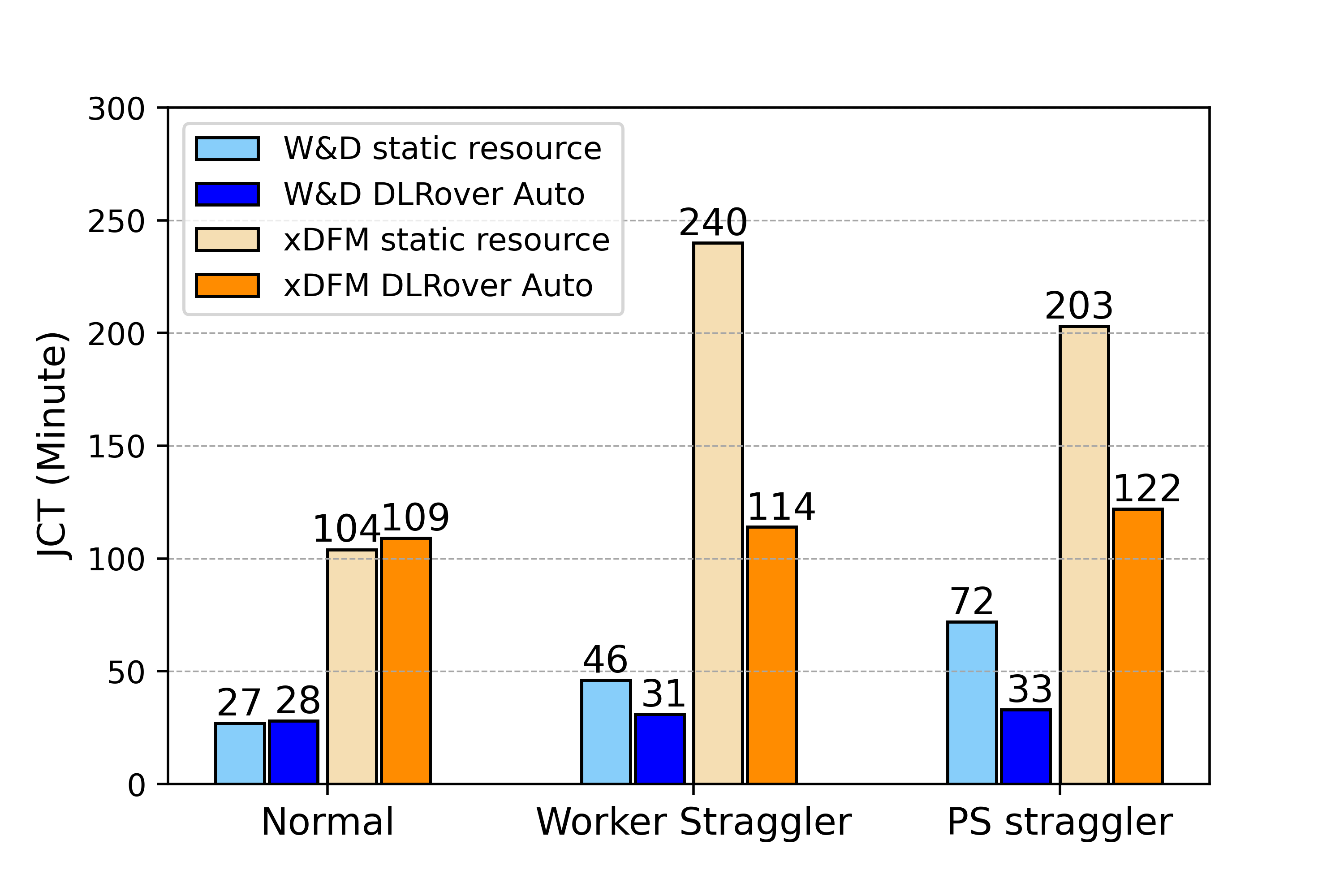
Figure 8. JCT of Training Jobs

6.3. Comparison with baselines

In this section, we compare DLRover with the heuristic auto-scaling algorithm (Or et al., 2020) and Optimus (Peng et al., 2018). Compared to algorithms used in DLRover, those two algorithms ignore the resources of each node and only add/remove fixed number of nodes each time. To be more specific, auto-scaling algorithm only add/remove workers and Optimus adds PS or workers each time. In the experiments, DLRover configures each PS and worker’s CPU resources according to Table 2. The auto-scaling algorithm adds/removes 4 workers for Wide & Deep jobs and 1 worker for xDeepFM jobs each time. The auto-scaling will add workers when the scaling efficiency (i.e., throughput improvement from a single new worker over existing single worker’s throughput) exceeds predefined threshold, which is 0.3 in our experiments. The original Optimus only adds one worker or PS each time. In order to speed up the adjustment, we make Optimus add 2 PS and 4 workers for Wide & Deep jobs and 1 PS and 1 worker for xDeepFM jobs. The interval of the adjustment in all experiments is 3min which contains about 20s to launch Pods, about 100s to initialize training and 60s to sample.

As shown in Figure 9(a) and Figure 9(c), DLRover can reach the job’s optimal resource much more quickly than auto-scaling and Optimus. For the Wide & Deep job, DLRover finishes the adjustment within 12min and has better throughput than the other two algorithms. The throughput of Wide & Deep job is limited by the number and CPU cores of PS and auto-scaling does not optimize PS at all. Optimus does add more PS but ignore the CPU cores of each PS. However there is a hot PS problem in Wide & Deep job that can not be resolved with more PS. Furthermore, DLRover reduces the JCT by more than 30% for Wide & Deep and 10% for xDeepFM (Figure 9(b) and Figure 9(d)).

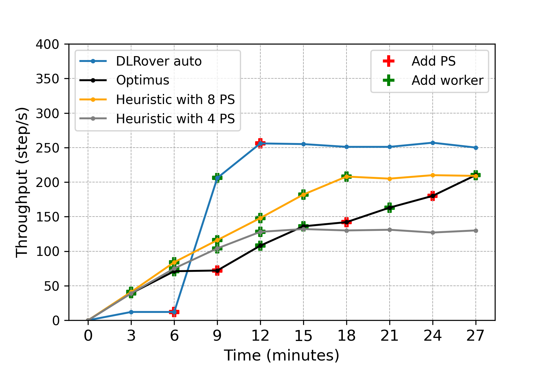
(a) W&D Throughput

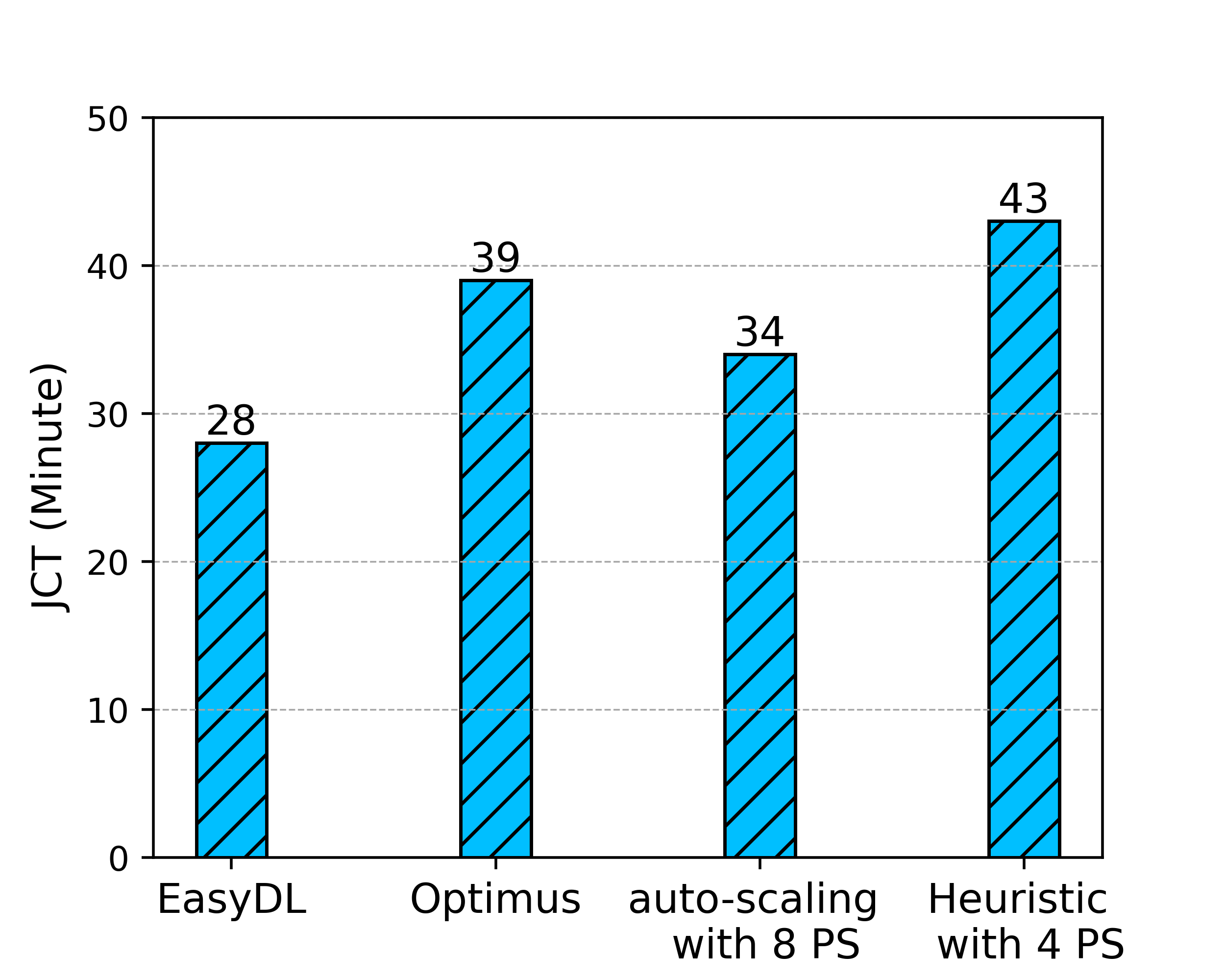
(b) W&D JCT

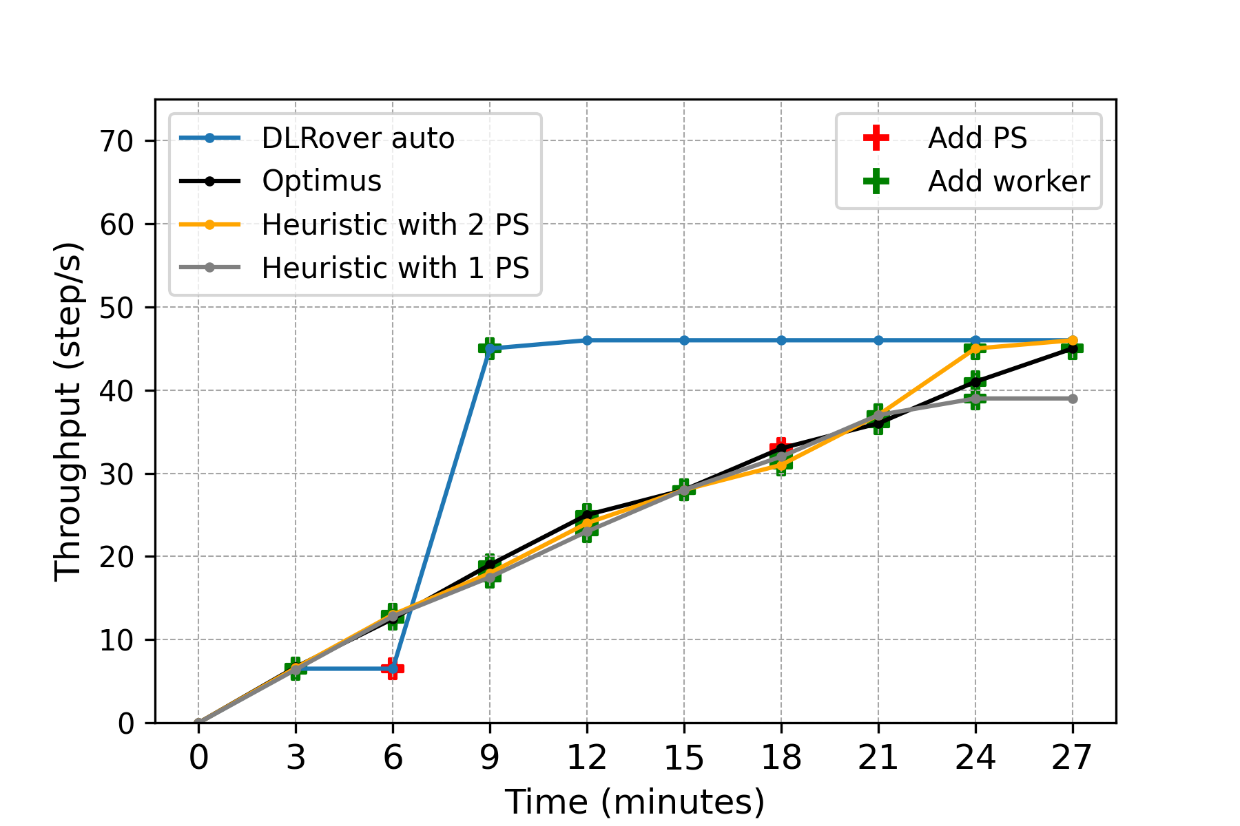
(c) xDFM Throughput

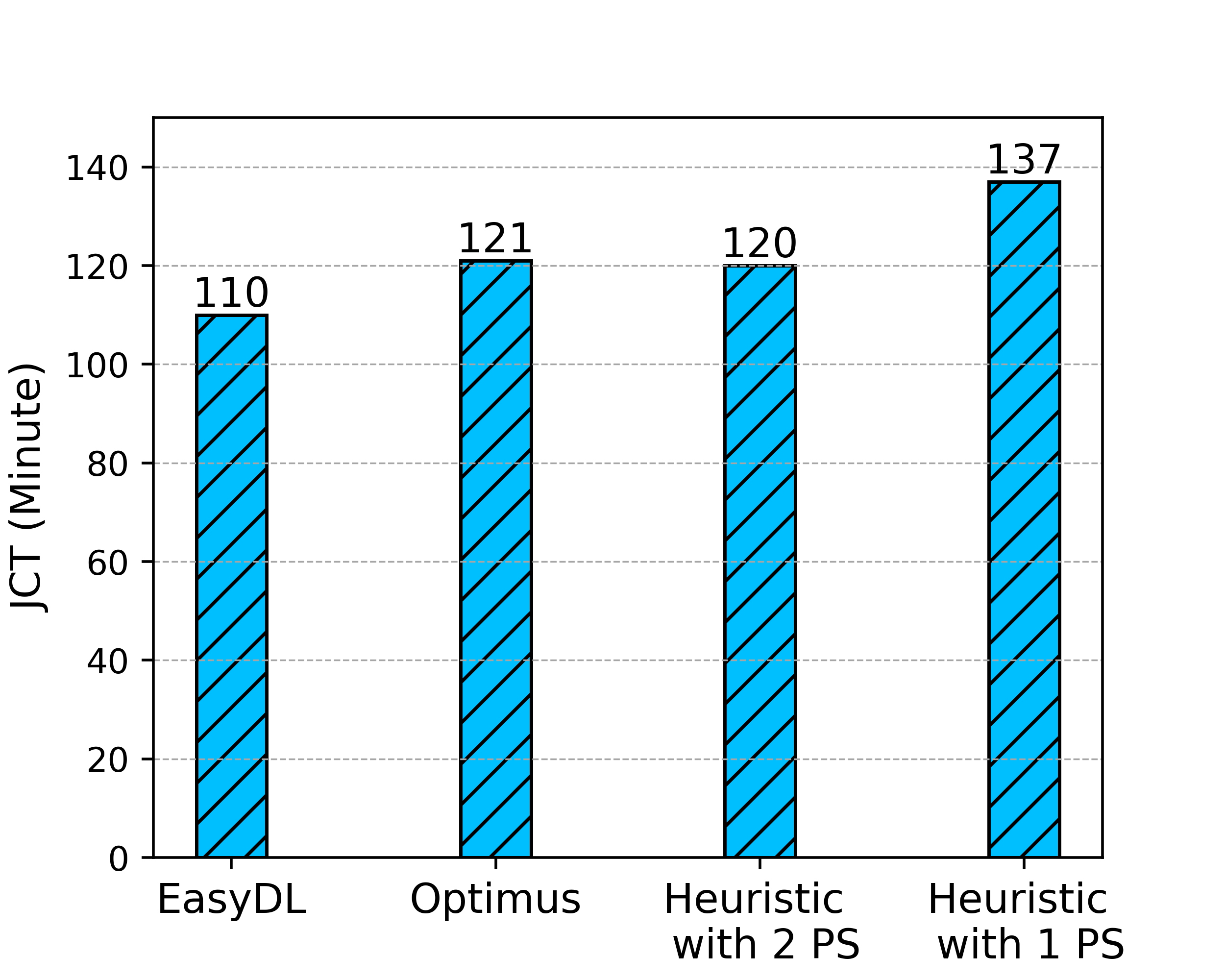
(d) xDFM JCT

Figure 9. Throughput and JCT

6.4. Cluster-level Improvement

DLRover is deployed on the production cluster of Ant Group to manage thousands of DL training jobs every day. We collect one-week statistics of jobs scheduled by TFJob in KubeFlow (George & Saha, 2022) with user manual resource configuration in June 2022, immediately before the deployment of DLRover, as the baseline. Then we collect another one-week statistics of jobs in August 2022 after DLRover is deployed in the cluster for weeks. The profiling of those jobs is shown in Table 3.

Job Statistic	TFJob	DLRover Auto
Job Count	5306	6109
Avg steps	268k	249k
Avg parameters	29.2 million	34.5 million
Avg dataset size	111 million	103 million

Table 3. Profiling of DL jobs of Ant Group

Optimization on JCT. As Figure 11 shows, DLRover can shorten the medium JCT of jobs by 31%. For jobs with hot PS problems, which occupies 13% of all jobs, DLRover can shorten the median JCT of those jobs by 21%. There are around 6% of jobs whose PS CPU utilization is more than 80%, which indicates they are not allocate enough CPU in PS initially. Those jobs’ JCT has been improved by 57% with the help of DLRover.

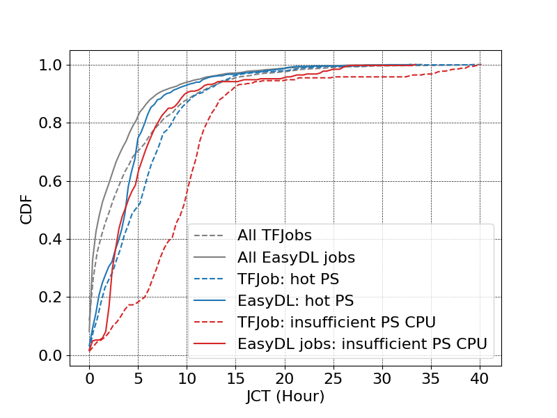
Figure 10. Jobs’ JCT.

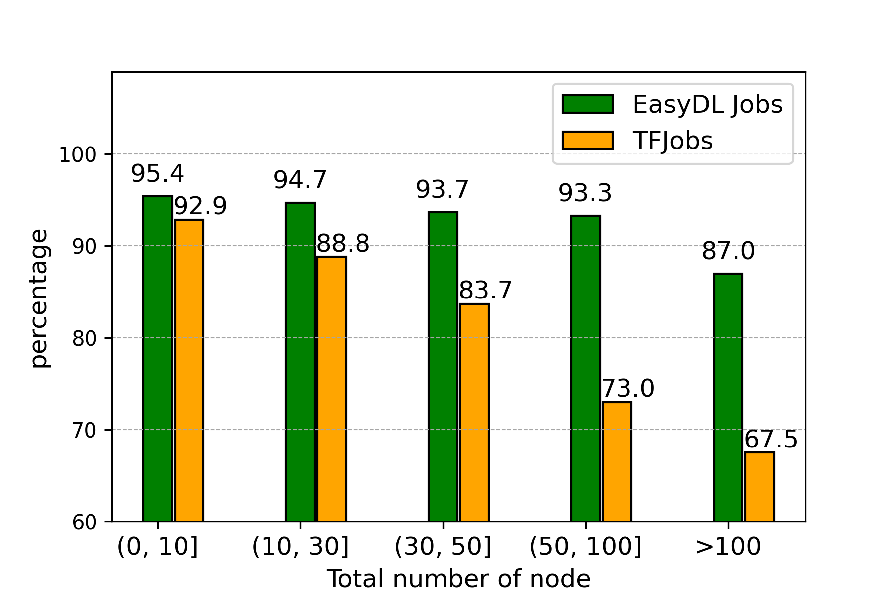
Figure 11. Jobs’ completion rate

Improvement in job completion rate. In the production cluster, many different types of jobs are running on the same machines for resources sharing, e.g., online services and DL training jobs. When online services require more resources, training jobs’ will be preempted since online services have higher priority. Before those jobs are marked as failure and users have to create new jobs. However, DLRover can avoid failure by launching new Pods on another machine to replace preempted Pods. This can significantly improve the completion rate compared to TFJob. As Figure 11 shows, DLRover has improved the completion rate significantly. Especially, jobs for large scale model training usually have more Pods and can benefit more from our system.

Improvement in resource utilization. In Ant Group, DL training jobs have used about 100,000 CPUs and 100TB memory daily. DLRover can improve the CPU utilization from 29% to 44% and memory utilization from 31% to 52% compared with manual resources configuration.

7. Related work

Automatic resource configuration. Automatic resource management is widely used in distributed data processing jobs on Hadoop (Shvachko et al., 2010) and Spark (Zaharia et al., 2012), machine learning jobs on Spark MLlib (Meng et al., 2016). Huang et al. (Huang et al., 2015) introduces an approach to configure the memory of large-scale ML in Spark automatically. On Spark or Hadoop, the machine learning algorithms are limited (e.g., logistic regression, SVM, and tree-based algorithm) and can be split into many small Map/Reduce tasks. The system can easily estimate the total required resources by measuring the resource requirements of a few tasks. However, deep learning jobs are running customized algorithms with DNN layers. Those automatic resource methods is not suitable for DL training.

There are already many efforts to automatically configuring the number of workers/parameter servers (Peng et al., 2018; Qiao et al., 2021; Gu et al., 2019). For workers, Pollux (Qiao et al., 2021) dynamically adjusts the number of workers and learning rate to improve throughput for synchronous SGD. However, they do not adjust the CPU and memory of each node, which are also key factors for the performance and non-failure of jobs. In the elasticity of Pollux and Tiresias, they re-deploy all workers when adjusting resource which will result in long transition time. In order to minimize the transition time, (Or et al., 2020) starts new allreduce operations only when new workers are ready and proposes a heuristic scaling to search the optimal number of workers.

For asynchronous training with PS architecture, Optimus (Peng et al., 2018) dynamically add one worker or parameter server each time to maximize the performance of the cluster without consideration of the transition time of elasticity. In a large-scaling training job, the transition time and search time is unaccepted because the number of workers and parameters is huge. Compared to Optimus, DLRover is designed to conduct elasticity in a more effective way with little overhead.

Elastic deep learning scheduling. Now, there are many DL frameworks to support elastic training. For elastic asynchronous training, the PS training of TensorFlow (Abadi & et al., 2015) supports scaling workers at runtime. Using checkpoint, TensorFlow also supports the elasticity of parameter servers. For elastic synchronous training, there are Elastic DL over multiple GPU (Wu et al., 2022), PyTorch-Elastic (PyTorch, 2020), and elastic Horovod (Sergeev & Balso, 2018). To support the scheduling of elastic training, existing systems need to restart the job by relaunching all Pods  (Peng et al., 2018; Qiao et al., 2021). What’s more, users need to implement their dynamic data partition for the change of workers. If the number of worker changes, the job need to repartition the whole dataset and restart an epoch  (Wu et al., 2022). The repartition may result in the inconsistency of sample iterations if the dataset is very huge. DLRover has a dynamic sharding service and doesn’t need to repartition during elasticity. Also, DLRover can keep consistency when adjusting parameter servers by checkpointing unused data shards and model parameters at the same time.

Straggler mitigation. In a distributed asynchronous SGD job using PS, the straggler may be a parameter server or worker. The Reason of straggler in a PS job includes: 1) hardware heterogeneity (Reiss et al., 2012), unbalanced data distribution and parameter distribution. Exist works mainly replace the slowest node with a new node to mitigate stragglers (Harlap et al., 2016; Or et al., 2020; Peng et al., 2018). This can not mitigate the straggler of parameter server resulted by unbalanced distribution across parameter servers. What’s more, Existing schedulers like Kubeflow (George & Saha, 2022) can only set the same CPU and memory for the worker or PS. DLRover  can set different resources for different pods based on elasticity to mitigate the bottleneck due to an unbalanced workload across Pods.

8. Conclusion

We have presented DLRover, a distributed DL system with automatic and dynamic resource configuration to improve training performance. Both the number of distributed nodes and the CPU/memory configuration of each node will be dynamically optimized during training jobs. After deploying DLRover to k8s clusters, we have greatly improved job completion time, job completion rate, and cluster resource utilization.

References

- Abadi & et al. (2015) Abadi, M. and et al., A. A. TensorFlow: Large-scale machine learning on heterogeneous systems, 2015. URL https://www.tensorflow.org/. Software available from tensorflow.org.
- Cheng et al. (2016) Cheng, H., Koc, L., Harmsen, J., Shaked, T., Chandra, T., Aradhye, H., Anderson, G., Corrado, G., Chai, W., Ispir, M., Anil, R., Haque, Z., Hong, L., Jain, V., Liu, X., and Shah, H. Wide & deep learning for recommender systems. In Karatzoglou, A., Hidasi, B., Tikk, D., Shalom, O. S., Roitman, H., Shapira, B., and Rokach, L. (eds.), Proceedings of the 1st Workshop on Deep Learning for Recommender Systems, DLRS@RecSys 2016, Boston, MA, USA, September 15, 2016, pp. 7–10. ACM, 2016. doi: 10.1145/2988450.2988454. URL https://doi.org/10.1145/2988450.2988454.
- George & Saha (2022) George, J. and Saha, A. End-to-end machine learning using kubeflow. In Dasgupta, G., Simmhan, Y., Srinivasan, B. V., Bhowmick, S., Singhee, A., Ramanath, M., Batra, N., and Prasad, A. S. (eds.), CODS-COMAD 2022: 5th Joint International Conference on Data Science & Management of Data (9th ACM IKDD CODS and 27th COMAD), Bangalore, India, January 8 - 10, 2022, pp. 336–338. ACM, 2022. doi: 10.1145/3493700.3493768. URL https://doi.org/10.1145/3493700.3493768.
- Gu et al. (2019) Gu, J., Chowdhury, M., Shin, K. G., Zhu, Y., Jeon, M., Qian, J., Liu, H., and Guo, C. Tiresias: A gpu cluster manager for distributed deep learning. In Proceedings of the 16th USENIX Conference on Networked Systems Design and Implementation, NSDI’19, pp. 485–500, USA, 2019. USENIX Association. ISBN 9781931971492.
- Harlap et al. (2016) Harlap, A., Cui, H., Dai, W., Wei, J., Ganger, G. R., Gibbons, P. B., Gibson, G. A., and Xing, E. P. Addressing the straggler problem for iterative convergent parallel ML. In Aguilera, M. K., Cooper, B., and Diao, Y. (eds.), Proceedings of the Seventh ACM Symposium on Cloud Computing, Santa Clara, CA, USA, October 5-7, 2016, pp. 98–111. ACM, 2016. doi: 10.1145/2987550.2987554. URL https://doi.org/10.1145/2987550.2987554.
- Huang et al. (2015) Huang, B., Boehm, M., Tian, Y., Reinwald, B., Tatikonda, S., and Reiss, F. R. Resource elasticity for large-scale machine learning. In Sellis, T. K., Davidson, S. B., and Ives, Z. G. (eds.), Proceedings of the 2015 ACM SIGMOD International Conference on Management of Data, Melbourne, Victoria, Australia, May 31 - June 4, 2015, pp. 137–152. ACM, 2015. doi: 10.1145/2723372.2749432. URL https://doi.org/10.1145/2723372.2749432.
- Jiang et al. (2020) Jiang, C., Qiu, Y., Shi, W., Ge, Z., Wang, J., Chen, S., Cerin, C., Ren, Z., Xu, G., and Lin, J. Characterizing co-located workloads in alibaba cloud datacenters. IEEE Transactions on Cloud Computing, pp. 1–1, 2020. doi: 10.1109/TCC.2020.3034500.
- Li et al. (2014) Li, M., Andersen, D. G., Park, J. W., Smola, A. J., Ahmed, A., Josifovski, V., Long, J., Shekita, E. J., and Su, B. Scaling distributed machine learning with the parameter server. In Flinn, J. and Levy, H. (eds.), 11th USENIX Symposium on Operating Systems Design and Implementation, OSDI ’14, Broomfield, CO, USA, October 6-8, 2014, pp. 583–598. USENIX Association, 2014. URL https://www.usenix.org/conference/osdi14/technical-sessions/presentation/li_mu.
- Lian et al. (2018) Lian, J., Zhou, X., Zhang, F., Chen, Z., Xie, X., and Sun, G. xdeepfm: Combining explicit and implicit feature interactions for recommender systems. In Guo, Y. and Farooq, F. (eds.), Proceedings of the 24th ACM SIGKDD International Conference on Knowledge Discovery & Data Mining, KDD 2018, London, UK, August 19-23, 2018, pp. 1754–1763. ACM, 2018. doi: 10.1145/3219819.3220023. URL https://doi.org/10.1145/3219819.3220023.
- Meng et al. (2016) Meng, X., Bradley, J. K., Yavuz, B., Sparks, E. R., Venkataraman, S., Liu, D., Freeman, J., Tsai, D. B., Amde, M., Owen, S., Xin, D., Xin, R., Franklin, M. J., Zadeh, R., Zaharia, M., and Talwalkar, A. Mllib: Machine learning in apache spark. J. Mach. Learn. Res., 17:34:1–34:7, 2016. URL http://jmlr.org/papers/v17/15-237.html.
- Naumov et al. (2019) Naumov, M., Mudigere, D., Shi, H. M., Huang, J., Sundaraman, N., Park, J., Wang, X., Gupta, U., Wu, C., Azzolini, A. G., Dzhulgakov, D., Mallevich, A., Cherniavskii, I., Lu, Y., Krishnamoorthi, R., Yu, A., Kondratenko, V., Pereira, S., Chen, X., Chen, W., Rao, V., Jia, B., Xiong, L., and Smelyanskiy, M. Deep learning recommendation model for personalization and recommendation systems. CoRR, abs/1906.00091, 2019. URL http://arxiv.org/abs/1906.00091.
- Or et al. (2020) Or, A., Zhang, H., and Freedman, M. J. Resource elasticity in distributed deep learning. In Dhillon, I. S., Papailiopoulos, D. S., and Sze, V. (eds.), Proceedings of Machine Learning and Systems 2020, MLSys 2020, Austin, TX, USA, March 2-4, 2020. mlsys.org, 2020. URL https://proceedings.mlsys.org/book/314.pdf.
- Peng et al. (2018) Peng, Y., Bao, Y., Chen, Y., Wu, C., and Guo, C. Optimus: An efficient dynamic resource scheduler for deep learning clusters. In Proceedings of the Thirteenth EuroSys Conference, EuroSys ’18, New York, NY, USA, 2018. Association for Computing Machinery. ISBN 9781450355841. doi: 10.1145/3190508.3190517. URL https://doi.org/10.1145/3190508.3190517.
- PyTorch (2020) PyTorch. Pytorch with elastic. https://pytorch.org/elastic/0.1.0rc2/overview.html, 2020.
- Qiao et al. (2021) Qiao, A., Choe, S. K., Subramanya, S. J., Neiswanger, W., Ho, Q., Zhang, H., Ganger, G. R., and Xing, E. P. Pollux: Co-adaptive cluster scheduling for goodput-optimized deep learning. In Brown, A. D. and Lorch, J. R. (eds.), 15th USENIX Symposium on Operating Systems Design and Implementation, OSDI 2021, July 14-16, 2021. USENIX Association, 2021. URL https://www.usenix.org/conference/osdi21/presentation/qiao.
- Reiss et al. (2012) Reiss, C., Tumanov, A., Ganger, G. R., Katz, R. H., and Kozuch, M. A. Heterogeneity and dynamicity of clouds at scale: Google trace analysis. In Carey, M. J. and Hand, S. (eds.), ACM Symposium on Cloud Computing, SOCC ’12, San Jose, CA, USA, October 14-17, 2012, pp. 7. ACM, 2012. doi: 10.1145/2391229.2391236. URL https://doi.org/10.1145/2391229.2391236.
- Sergeev & Balso (2018) Sergeev, A. and Balso, M. D. Horovod: fast and easy distributed deep learning in tensorflow. CoRR, abs/1802.05799, 2018. URL http://arxiv.org/abs/1802.05799.
- Shvachko et al. (2010) Shvachko, K., Kuang, H., Radia, S., and Chansler, R. The hadoop distributed file system. In Khatib, M. G., He, X., and Factor, M. (eds.), IEEE 26th Symposium on Mass Storage Systems and Technologies, MSST 2012, Lake Tahoe, Nevada, USA, May 3-7, 2010, pp. 1–10. IEEE Computer Society, 2010. doi: 10.1109/MSST.2010.5496972. URL https://doi.org/10.1109/MSST.2010.5496972.
- Wu et al. (2022) Wu, Y., Ma, K., Yan, X., Liu, Z., Cai, Z., Huang, Y., Cheng, J., Yuan, H., and Yu, F. Elastic deep learning in multi-tenant gpu clusters. IEEE Transactions on Parallel and Distributed Systems, 33(1):144–158, 2022. doi: 10.1109/TPDS.2021.3064966.
- Zaharia et al. (2012) Zaharia, M., Chowdhury, M., Das, T., Dave, A., Ma, J., McCauly, M., Franklin, M. J., Shenker, S., and Stoica, I. Resilient distributed datasets: A fault-tolerant abstraction for in-memory cluster computing. In 9th USENIX Symposium on Networked Systems Design and Implementation (NSDI 12), pp. 15–28, San Jose, CA, April 2012. USENIX Association. ISBN 978-931971-92-8.