VNE: An Effective Method for Improving Deep Representation
by Manipulating Eigenvalue Distribution

Abstract

Since the introduction of deep learning, a wide scope of representation properties, such as decorrelation, whitening, disentanglement, rank, isotropy, and mutual information, have been studied to improve the quality of representation. However, manipulating such properties can be challenging in terms of implementational effectiveness and general applicability. To address these limitations, we propose to regularize von Neumann entropy (VNE) of representation. First, we demonstrate that the mathematical formulation of VNE is superior in effectively manipulating the eigenvalues of the representation autocorrelation matrix. Then, we demonstrate that it is widely applicable in improving state-of-the-art algorithms or popular benchmark algorithms by investigating domain-generalization, meta-learning, self-supervised learning, and generative models. In addition, we formally establish theoretical connections with rank, disentanglement, and isotropy of representation. Finally, we provide discussions on the dimension control of VNE and the relationship with Shannon entropy. Code is available at: https://github.com/jaeill/CVPR23-VNE.

1 Introduction

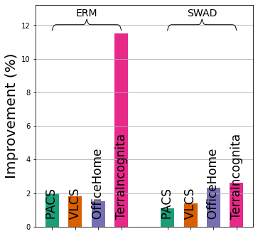
(a)

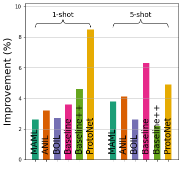
(b)

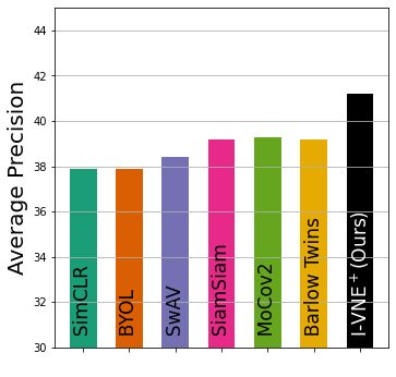
(c)

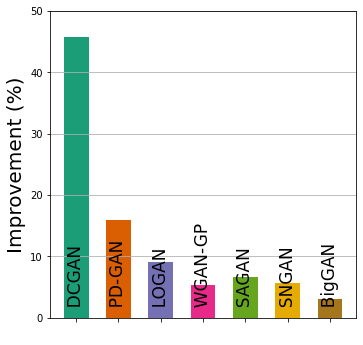
(d)

Figure 1: General applicability of VNE: performance of state-of-the-art algorithms or popular benchmark algorithms can be further improved by regularizing von Neumann entropy (full result tables will be provided in Section 3). (a) Domain generalization: relative improvements over ERM and SWAD (current state-of-the-art). (b) Meta-learning: relative improvements over six popular benchmark algorithms. (c) Self-supervised learning: performance comparison against the current state-of-the-art algorithms for COCO detection. (d) GAN: relative improvements in Fréchet Inception Distance (FID) for seven popular benchmark algorithms.

Improving the quality of deep representation by pursuing a variety of properties in the representation has been adopted as a conventional practice. To learn representations with useful properties, various methods have been proposed to manipulate the representations. For example, decorrelation reduces overfitting, enhances generalization in supervised learning [20, 92], and helps in clustering [79]. Whitening improves convergence and generalization in supervised learning [44, 45, 23, 60], improves GAN stability [76], and helps in domain adaptation [73]. Disentanglement was proposed as a desirable property of representations [9, 1, 42]. Increasing rank of representations was proposed to resolve the dimensional collapse phenomenon in self-supervised learning [43, 47]. Isotropy was proposed to improve the downstream task performance of BERT-based models in NLP tasks [56, 78]. Preventing informational collapse (also known as representation collapse) was proposed as a successful learning objective in non-contrastive learning [7, 96]. In addition, maximizing mutual information was proposed as a successful learning objective in contrastive learning [39, 69, 80].

Although aforementioned properties are considered as desirable for useful representations, typical implementational limitations, such as dependency to specific architectures or difficulty in proper loss formulation, inhibited the properties from being more popularly adopted. For example, the methods for whitening [44, 45, 23, 60, 76, 73], isotropy [56, 78], and rank [43] are typically dependent on specific architectures (e.g., decorrelated batch normalization [44] and normalizing flow [56]). Regarding disentanglement and mutual information, loss formulations are not straightforward because measuring disentanglement generally relies on external models [41, 27, 51, 13, 32] or is tuned for a specific dataset [50] and formulating mutual information in high-dimensional spaces is notoriously difficult [82] and only tractable lower bound can be implemented by training additional critic functions [71]. Meanwhile, several decorrelation methods [20, 92, 7, 96] have implemented model-agnostic and straightforward loss formulations that minimize the Frobenius norm between the autocorrelation matrix $\mathcal{C}_{\text{auto}}$ (or crosscorrelation matrix $\mathcal{C}_{\text{cross}}$) and a scale identity matrix $c\cdot I$ for an appropriate $c>0$. Because of the easiness of enforcing decorrelation via a simple loss formulation, these decorrelation methods can be considered to be generally applicable to a wide scope of applications. However, the current implementation of the loss as a Frobenius norm can exhibit undesirable behaviors during learning and thus fail to have a positive influence as we will explain further in Section 2.4.

To address the implementational limitations, this study considers the eigenvalue distribution of the autocorrelation matrix $\mathcal{C}_{\text{auto}}$. Because $\mathcal{C}_{\text{auto}}$ converges to scalar identity matrix $c\cdot I$ for an appropriate $c>0$ if and only if the eigenvalue distribution of $\mathcal{C}_{\text{auto}}$ converges to a uniform distribution, it is possible to control the eigenvalue distribution using methods that are different from Frobenius norm. To this end, we adopt a mathematical formulation from quantum information theory and introduce von Neumann entropy (VNE) of deep representation, a novel method that directly controls the eigenvalue distribution of $\mathcal{C}_{\text{auto}}$ via an entropy function. Because entropy function is an effective measure for the uniformity of underlying distribution and can handle extreme values, optimizing the entropy function is quite stable and does not possess implementational limitations of previous methods.

In addition to the effectiveness of VNE on manipulating the eigenvalue distribution of $\mathcal{C}_{\text{auto}}$, we demonstrate that regularizing VNE is widely beneficial in improving the existing studies. As summarized in Figure 1, performance improvement is significant and consistent. Moreover, theoretical connections between VNE and the popular representation properties are formally proven and support the empirical superiority. Thanks to the implementational effectiveness and theoretical connections, VNE regularizer can effectively control not only von Neumann entropy but also other theoretically related properties, including rank and isotropy. Our contributions can be summarized as below:

• We introduce a novel representation regularization method, von Neumann entropy of deep representation.

• We describe VNE’s implementational effectiveness (in Section 2).

• We demonstrate general applicability of VNE by improving current state-of-the-art methods in various tasks and achieving a new state-of-the-art performance in self-supervised learning and domain generalization (in Section 3).

• We provide theoretical connections by proving that VNE is theoretically connected to rank, disentanglement, and isotropy of representation (in Section 4).

2 Implementational Effectiveness of VNE

Even though the von Neumann entropy originates from quantum information theory, we focus on its mathematical formulation to understand why it is effective for manipulating representation properties. We start by defining the autocorrelation matrix.

2.1 Autocorrelation of Representation

For a given mini-batch of $N$ samples, the representation matrix can be denoted as $\bm{H}=[\bm{h}_{1},\bm{h}_{2},...,\bm{h}_{N}]^{T}\in\mathbb{R}^{N\times d}$, where $d$ is the size of the representation vector. For simplicity, we assume $L_{2}$-normalized representation vectors satisfying $||\bm{h}_{i}||_{2}=1$ as in [87, 70, 75, 58, 86, 62, 93]. Then, the autocorrelation matrix of the representation is defined as:

$$\mathcal{C}_{\text{auto}}\triangleq\sum_{i=1}^{N}\frac{1}{N}\bm{h}_{i}\bm{h}_{i}^{T}=\bm{H}^{T}\bm{H}/N.\vspace{-0.3cm}$$ (1)

For $\mathcal{C}_{\text{auto}}$’s eigenvalues $\{\lambda_{j}\}$, it can be easily verified that $\sum_{j}\lambda_{j}=1$ and $\forall_{j}~{}\lambda_{j}\geq 0$ because $||\bm{h}_{i}||_{2}=1$ and $\mathcal{C}_{\text{auto}}\geq 0$. For the readers familiar with quantum information theory, $\mathcal{C}_{\text{auto}}$ is used in place of the density matrix $\rho$ of Supplementary A (a brief introduction to quantum theory).

$\mathcal{C}_{\text{auto}}$ is closely related to a variety of representation properties. In the extreme case of $\mathcal{C}_{\text{auto}}\rightarrow c\cdot I_{d}$, where $c$ is an adequate positive constant, the eigenvalue distribution of $\mathcal{C}_{\text{auto}}$ becomes perfectly uniform. Then, the representation $\bm{h}$ becomes decorrelated [20], whitened [44], full rank [43], and isotropic [84]. In the case of self-supervised learning, it means prevention of informational collapse[7, 96].

Besides its relevance to numerous representation properties, regularizing $\mathcal{C}_{\text{auto}}$ is of a great interest because it permits a simple implementation. Unlike many of the existing implementations that can be dependent on specific architecture or dataset, difficult to implement as a loss, or dependent on successful learning of external models, $\mathcal{C}_{\text{auto}}$ can be regularized as a simple penalty loss. Because $\mathcal{C}_{\text{auto}}$ is closely related to a variety of representation properties and because it permits a broad applicability, we focus on $\mathcal{C}_{\text{auto}}$ in this study.

2.2 Regularization with Frobenius Norm

A popular method for regularizing the eigenvalues of $\mathcal{C}_{\text{auto}}$ is to implement the loss of Frobenius norm as shown below.

$$\begin{split}\mathcal{L}_{\text{Frobenius}}&\triangleq||\mathcal{C}_{\text{auto}}-c\cdot I_{d}||_{F}^{2}\\ &=\sum_{i}(\mathcal{C}_{i,i}-c)^{2}+\sum_{i}\sum_{j\neq i}\mathcal{C}_{i,j}^{2}\end{split}\vspace{-0.5cm}$$ (2)

$\mathcal{C}_{i,j}$ is the $(i,j)$ element of $\mathcal{C}_{\text{auto}}$ and $c$ is an adequate positive constant. While this approach has been widely adopted in the previous studies including DeCov [20], cw-CR [19], SDC [92], Barlow Twins [96], and VICReg [7], it can be ineffective for controlling eigenvalues as we will show in Section 2.4.

2.3 Regularization with Von Neumann Entropy

Von Neumann entropy of autocorrelation is defined as the Shannon entropy over the eigenvalues of $\mathcal{C}_{\text{auto}}$. The mathematical formulation is shown below.

$$S(\mathcal{C}_{\text{auto}})\triangleq-\sum_{j}\lambda_{j}\log{\lambda_{j}}.\vspace{-0.2cm}$$ (3)

As shown in Lemma 1 of Supplementary B, $S(\mathcal{C}_{\text{auto}})$ ranges between zero and $\log{d}$. Implementing of VNE regularization is simple. When training an arbitrary task $\mathcal{T}$, we can subtract $\alpha\cdot S(\mathcal{C}_{\text{auto}})$ from the main loss $\mathcal{L}_{\mathcal{T}}$.

$$\mathcal{L}_{\mathcal{T}\text{+VNE}}=\mathcal{L}_{\mathcal{T}}-\alpha\cdot S(\mathcal{C}_{\text{auto}}).\vspace{-0.1cm}$$ (4)

Note that training $\mathcal{T}$ with $\mathcal{L}_{\mathcal{T}\text{+VNE}}$ is denoted as VNE⁺ if $\alpha>0$, VNE^- if $\alpha<0$, and Vanilla if $\alpha=0$. The PyTorch implementation of $S(\mathcal{C}_{\text{auto}})$ can be found in Figure 10 of Supplementary C. Computational overhead of VNE calculation is light, as demonstrated in Table 9 of Supplementary D.

2.4 Frobenius Norm vs. Von Neumann Entropy

The formulation of von Neumann entropy in Eq. (3) exhibits two distinct differences when compared to the formulation of Frobenius norm in Eq. (2). First, while Frobenius norm deals with all the elements of $\mathcal{C}_{\text{auto}}\in\mathbb{R}^{d\times d}$, VNE relies on an eigenvalue decomposition to identify the eigenvalues of the current model under training and focuses on the current $d$ eigenvalues only. Second, while Frobenius norm can manifest an undesired behavior when some of the eigenvalues are zero and cannot be regulated toward $c$, VNE gracefully handles such dimensions because $0\cdot\log{0}=0$.

To demonstrate our points, we have performed a supervised learning with ResNet-18 and three datasets. The results are shown in Table 1 where regularization with Frobenius norm causes many neurons to become dead. Instead of focusing on the eigenvalues, Frobenius norm takes a shortcut of making many of the $d=512$ dimensions unusable and fails to recover. Note that VNE⁺ and VNE^- do not present such a degenerate behavior. We have repeated the supervised experiment with ResNet-18, but this time using a relatively sophisticated dataset of ImageNet-1K. The distribution of eigenvalues are shown in Figure 2(a) where Frobenius norm fails to affect the distribution. VNE⁺ and VNE^-, however, successfully make the distribution more uniform and less uniform, respectively. Finally, the learning history of Frobenius norm loss for a self-supervised learning is shown in Figure 2(b). While Barlow Twins [96] is a well-known method, the Frobenius norm loss can be better manipulated by regularizing VNE⁺ instead of regularizing the Frobenius norm itself.

Method	Dead units
	CIFAR-10	STL-10	CIFAR-100
Vanilla	0	0	0
VNE-	0	0	1
VNE+	2	0	1
$\mathcal{L}_{\text{Frobenius}}$	447	365	325

Table 1: Count of dead units (dead neurons) when training ResNet-18 with the standard cross-entropy loss. The penultimate layer’s representation with $d=512$ was analyzed.

(a)

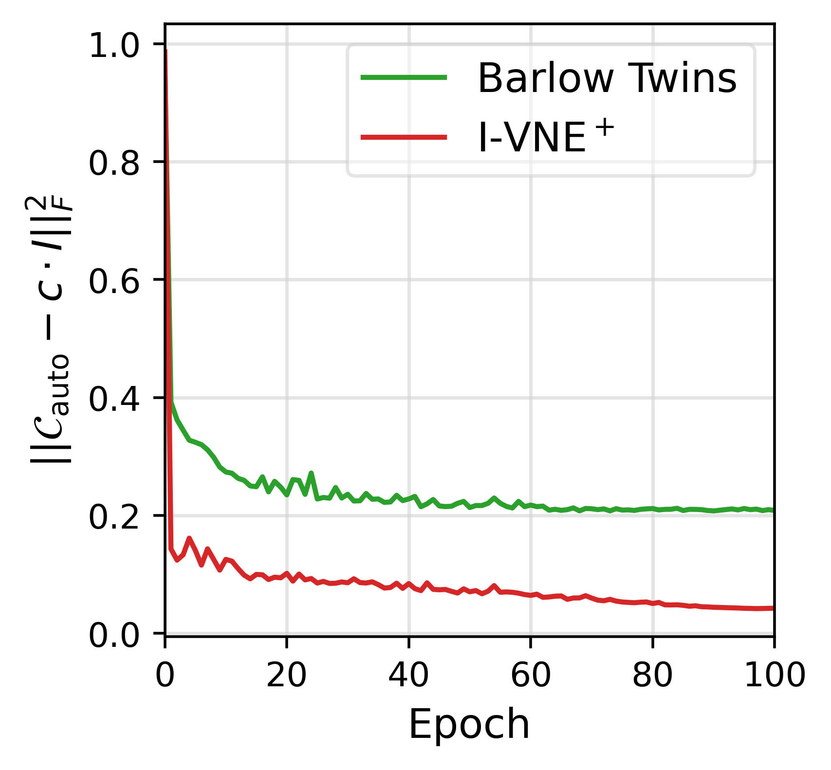
(b)

Figure 2: (a) Eigenvalue distribution when training ResNet-18 with the standard cross-entropy loss (dataset: ImageNet-1K, $d=512$). (b) Frobenius norm when performing self-supervised learning with ResNet-18. I-VNE⁺ will be explained further in Section 3.3.

3 General Applicability of VNE: Experiments

In this section, we demonstrate the general applicability of VNE by investigating some of the existing representation learning tasks. Although the results for meta-learning, self-supervised learning (SSL), and GAN can be supported by the theoretical connections between VNE and the popular representation properties presented in Section 4, result for domain generalization (DG) is quite surprising. We will discuss the fundamental difference of DG in Section 5.1.

3.1 Domain Generalization: Enhancing Generalization

Given multi-domain datasets, domain generalization attempts to train models that predict well on unseen data distributions [4]. In this section, we demonstrate the effectiveness of VNE on ERM [36], one of the most competitive algorithms in DomainBed [36], and on SWAD [12], which is the state-of-the-art algorithm. To reproduce the algorithms, we train ERM and SWAD based on an open source in [36, 12]. VNE is calculated for the penultimate representation of ResNet-50 models. Our experiments are performed in leave-one-domain-out setting [36] with the most popular datasets (PACS[57], VLCS[28], OfficeHome[83], and TerraIncognita[8]).

We have analyzed the eigenvalue distribution of $\mathcal{C}_{\text{auto}}$, and the results are presented in Figure 3. At first glance, VNE⁺ and VNE^- successfully make the eigenvalue distribution more uniform and less uniform, respectively in Figure 3(a). The corresponding von Neumann entropies are certainly increased by VNE⁺ and decreased by VNE^- in Figure 3(b). When we take a deeper look at the eigenvalues of Vanilla (we count the number of eigenvalues larger than 1e-4), we observe that DG naturally utilizes a small number of eigenvalues (3% of total). In this context, we can hypothesize that DG prefers utilizing a relatively small number of dimensions. In addition, the empirical results support the hypothesis. In Table 2, VNE^- improves all the benchmarks trained with ERM algorithm in four popular datasets. In Table 3, VNE^- also improves all the benchmarks trained with SWAD algorithm. Furthermore, the resulting performance is the state-of-the-art because SWAD is the current state-of-the-art algorithm.

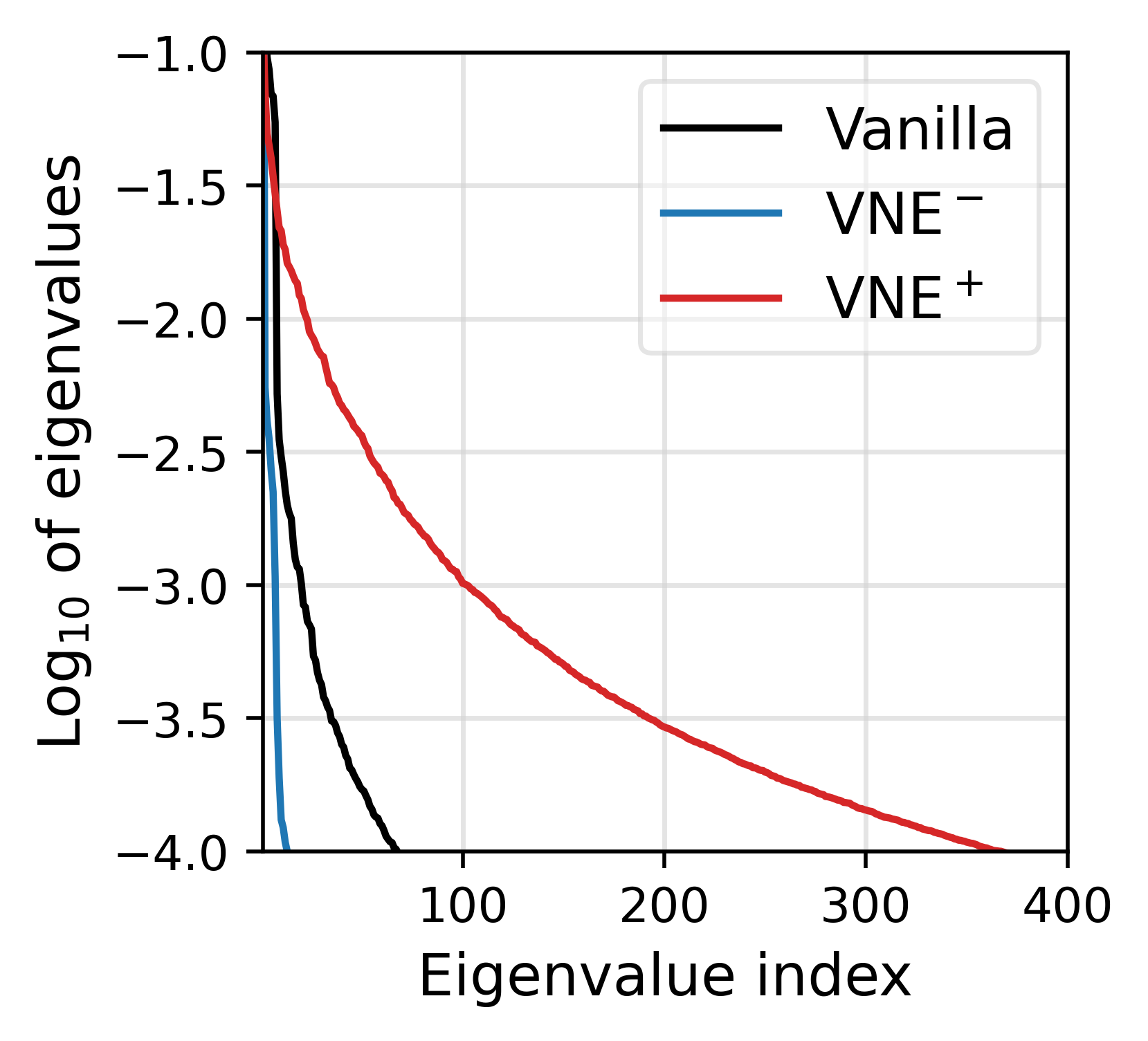
(a)

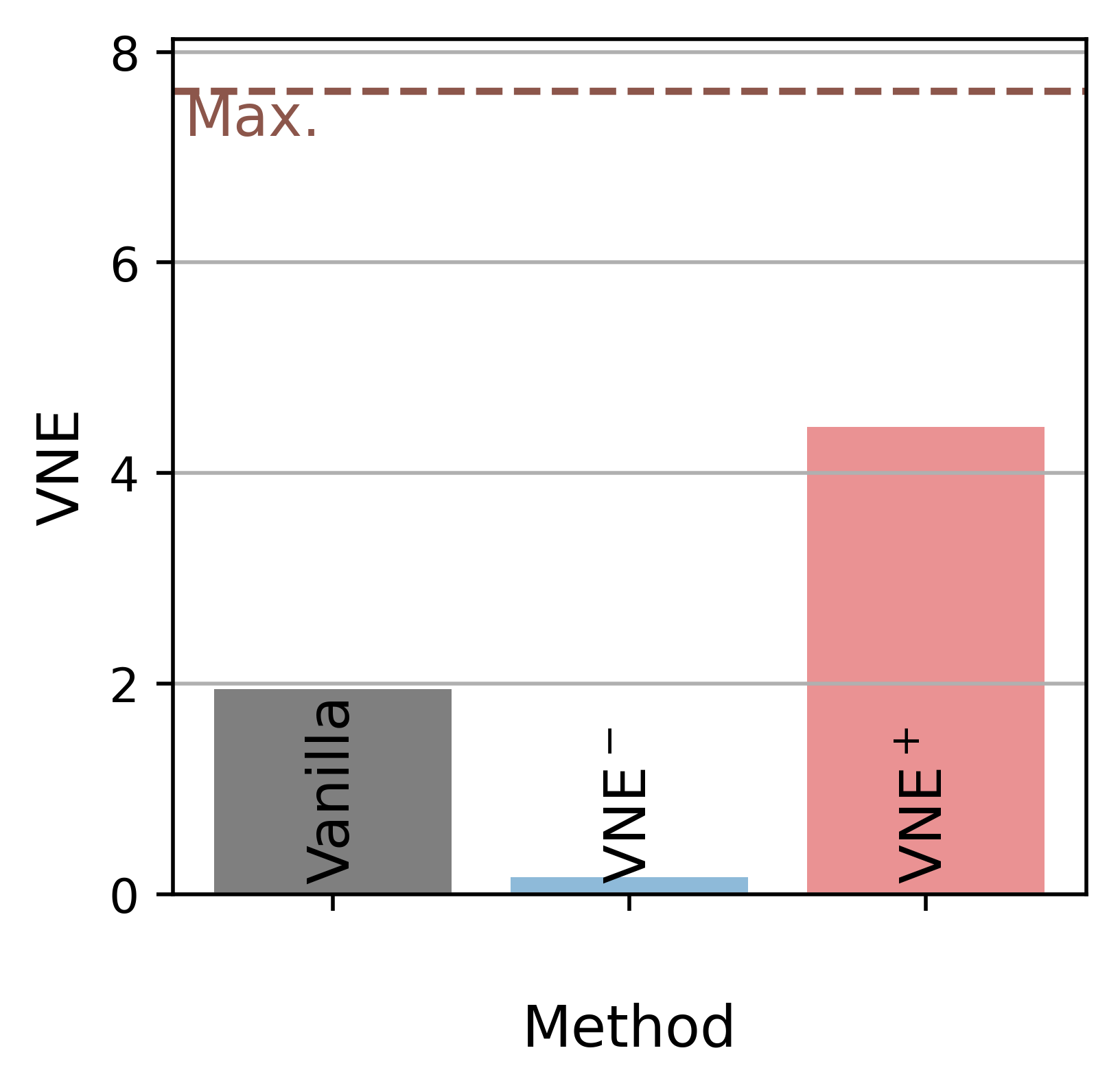
(b)

Figure 3: Domain Generalization: In (a), Eigenvalues of $\mathcal{C}_{\text{auto}}$ are presented in log₁₀ scale and descending order. In (b), von Neumann entropies are presented. ResNet-50 encoders are trained by the ERM [36] algorithm with the PACS dataset for 5000 steps. Each representation has a dimension of 2048.

Dataset	Method	Accuracy per test domain				Avg.	Diff.
PACS		A	C	P	S
	Vanilla	87.6	79.7	95.9	77.6	85.2
	VNE+	82.4	79.2	96.6	70.9	82.3	-2.9
	VNE-	88.6	79.9	96.7	82.3	86.9	1.7
VLSC		C	L	S	V
	Vanilla	98.9	61.5	70.3	76.1	76.7
	VNE+	96.6	65.5	70.1	75.2	76.8	0.1
	VNE-	97.5	65.9	70.4	78.4	78.1	1.4
OfficeHome		A	C	P	R
	Vanilla	57.9	52.5	75.5	73.5	64.9
	VNE+	59.6	50.7	73.1	74.4	64.4	-0.5
	VNE-	60.4	54.7	73.7	74.7	65.9	1.0
TerraIncognita		L100	L38	L43	L46
	Vanilla	50.4	42.0	56.8	32.3	45.4
	VNE+	50.3	38.1	55.4	33.6	44.3	-1.1
	VNE-	58.1	42.9	58.1	43.5	50.6	5.2

Table 2: Domain Generalization: Performance evaluation of models trained with ERM algorithm and various datasets.

Dataset	Method	Accuracy per test domain				Avg.	Diff.
PACS		A	C	P	S
	Vanilla	89.2	83.3	97.9	82.5	88.2
	VNE+	87.9	80.6	97.3	78.8	86.2	-2.1
	VNE-	90.1	83.8	97.5	81.8	88.3	0.1
VLCS		C	L	S	V
	Vanilla	98.9	64.5	74.6	79.7	79.4
	VNE+	98.7	62.9	74.9	80.5	79.2	-0.2
	VNE-	99.2	63.7	74.4	81.6	79.7	0.3
OfficeHome		A	C	P	R
	Vanilla	64.6	57.7	78.4	80.1	70.2
	VNE+	65.3	57.6	78.6	80.5	70.5	0.3
	VNE-	66.6	58.6	78.9	80.5	71.1	0.9
TerraIncognita		L100	L38	L43	L46
	Vanilla	58.2	45.1	60.9	39.4	50.9
	VNE+	45.3	37.7	60.7	40.5	46.1	-4.8
	VNE-	59.9	45.5	59.6	41.9	51.7	0.8

Table 3: Domain Generalization: Performance evaluation of models trained with SWAD algorithm and with various datasets. State-of-the-art performances are indicated in bold.

3.2 Meta-Learning: Enhancing Generalization

Given meta tasks during the meta-training phase, meta-learning attempts to train meta learners that can generalize well to unseen tasks with just few examples during the meta-testing phase. In this section, we present the effectiveness of VNE on the most prevalent meta-learning algorithms - MAML [29], ANIL [72], BOIL [68], ProtoNet [77], Baseline [16], and Baseline++ [16]. To reproduce the algorithms, we train Baseline, Baseline++, and ProtoNet based on an open source code base in [16] and train MAML, ANIL, and BOIL using torchmeta [22]. VNE is calculated for the penultimate representation of the standard 4-ConvNet models. Our experiments are performed in 5-way 1-shot and in 5-way 5-shot with the mini-ImageNet [85], a standard benchmark dataset in few-shot learning.

Similar to domain generalization, we have analyzed the eigenvalue distribution of $\mathcal{C}_{\text{auto}}$, and the results are presented in Figure 4. At first glance, VNE⁺ and VNE^- successfully make the eigenvalue distribution more uniform and less uniform, respectively in Figure 4(a). The corresponding von Neumann entropies are certainly increased by VNE⁺ and decreased by VNE^- in Figure 4(b). When we take a deeper look at the eigenvalues of Vanilla, we observe that meta-learning naturally utilizes a large number of eigenvalues (94% of total). In this context, we can hypothesize that meta-learning prefers utilizing a relatively large number of dimensions. In addition, the hypothesis is supported by the empirical results where all of six popular benchmark algorithms in both 5-way 1-shot and 5-way 5-shot settings are improved by VNE⁺ in Table 4. Note that VNE⁺ consistently provides a gain for all the meta-learning benchmarks that we have investigated.

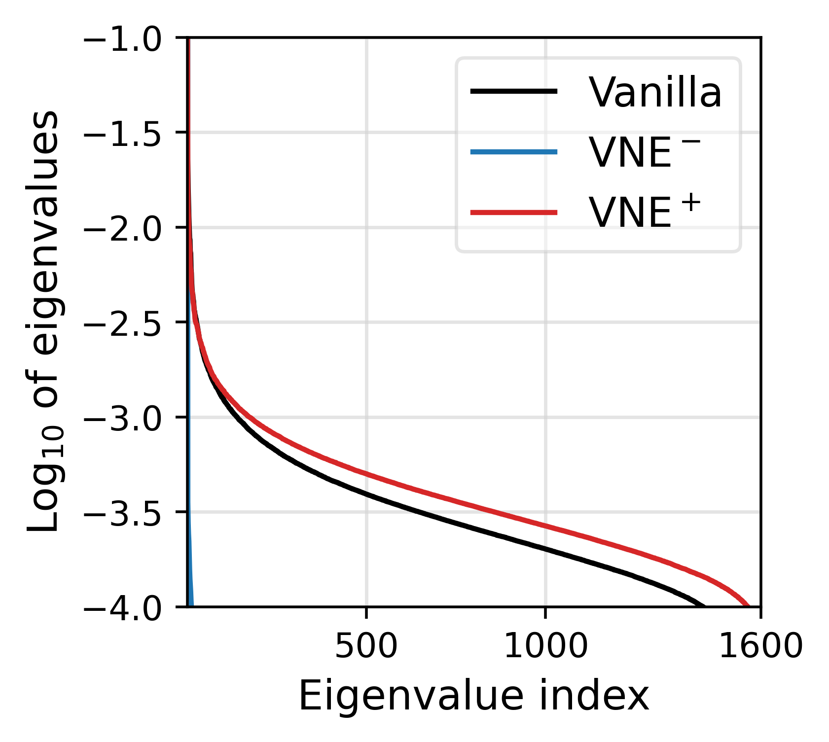
(a)

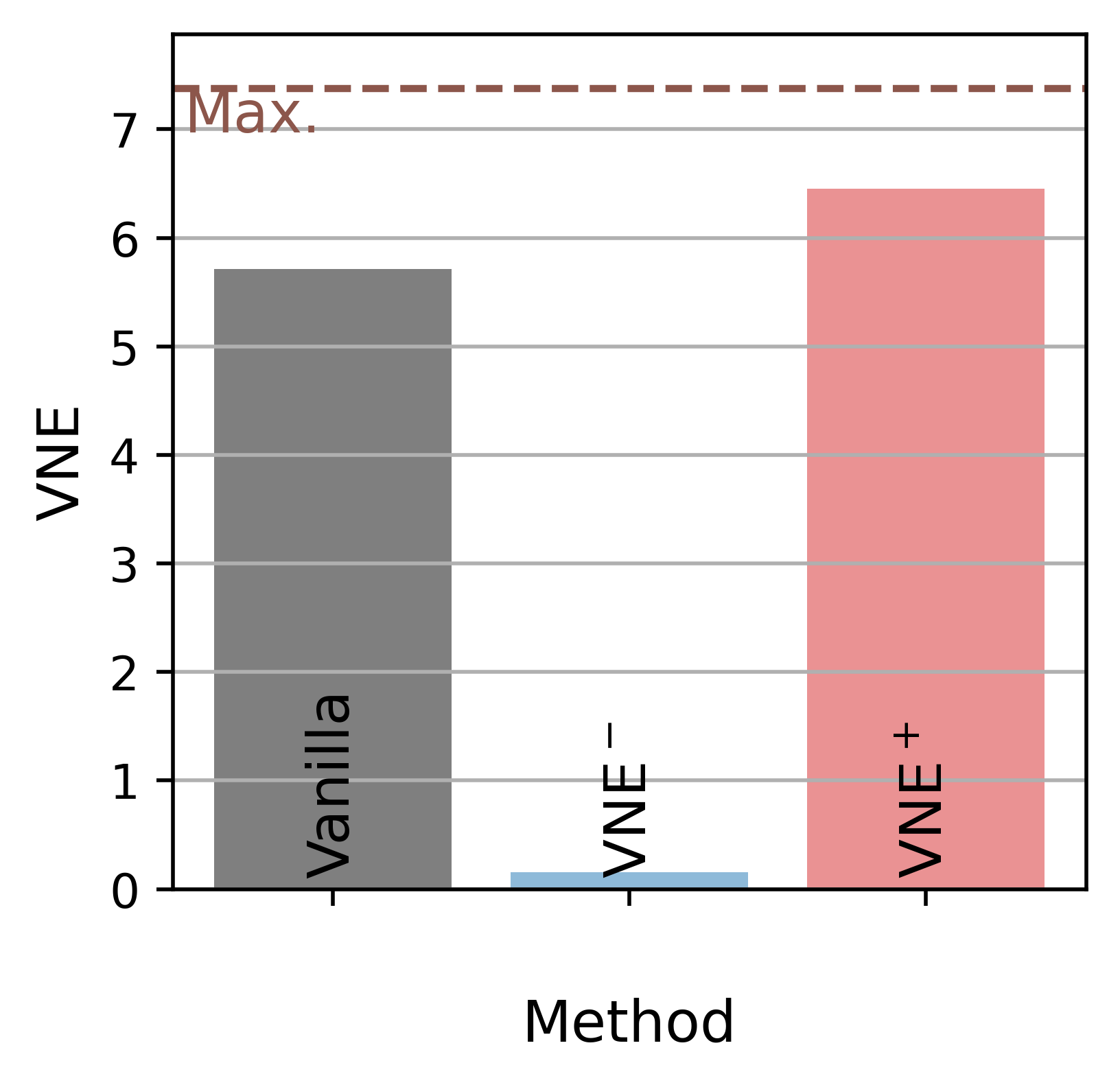
(b)

Figure 4: Meta-learning: In (a), Eigenvalues of $\mathcal{C}_{\text{auto}}$ are presented in log₁₀ scale and descending order. In (b), von Neumann entropies are presented. 4-ConvNet models are trained by the Baseline [16] algorithm with mini-ImageNet for 100 epochs. Each representation has a dimension of 1600.

Method		1-shot		5-shot
		Avg. Acc. (%)	Diff.	Avg. Acc. (%)	Diff.
MAML [29]	Vanilla	48.86 $\pm$ 0.82		64.59 $\pm$ 0.88
	VNE-	46.84 $\pm$ 0.76	-2.02	62.57 $\pm$ 0.76	-2.02
	VNE+	50.14 $\pm$ 0.77	1.28	66.42 $\pm$ 0.57	1.83
ANIL [72]	Vanilla	46.70 $\pm$ 0.40		61.50 $\pm$ 0.50
	VNE-	45.40 $\pm$ 0.52	-1.30	60.14 $\pm$ 0.56	-1.36
	VNE+	48.20 $\pm$ 0.45	1.50	63.42 $\pm$ 0.45	1.92
BOIL [68]	Vanilla	49.61 $\pm$ 0.16		66.46 $\pm$ 0.37
	VNE-	48.42 $\pm$ 0.34	-1.19	65.34 $\pm$ 0.45	-1.12
	VNE+	50.95 $\pm$ 0.42	1.34	67.52 $\pm$ 0.46	1.06
Baseline [16]	Vanilla	45.41 $\pm$ 0.72		62.53 $\pm$ 0.69
	VNE-	30.43 $\pm$ 0.72	-14.98	48.03 $\pm$ 0.90	-14.50
	VNE+	47.03 $\pm$ 0.73	-01.62	65.85 $\pm$ 0.67	-03.32
Baseline++ [16]	Vanilla	47.95 $\pm$ 0.74		66.43 $\pm$ 0.63
	VNE-	29.52 $\pm$ 0.76	-18.43	60.98 $\pm$ 0.78	-5.45
	VNE+	50.17 $\pm$ 0.77	-02.22	67.25 $\pm$ 0.67	0.82
ProtoNet [77]	Vanilla	43.16 $\pm$ 0.55		64.24 $\pm$ 0.72
	VNE-	-		62.14 $\pm$ 0.69	-2.10
	VNE+	46.81 $\pm$ 0.35	3.65	66.72 $\pm$ 0.71	2.48

Table 4: Meta-learning: Performance evaluation of 5-way 1-shot and 5-way 5-shot with mini-ImageNet.

3.3 SSL: Preventing Representation Collapse

Given an unlabelled dataset, self-supervised learning attempts to learn representation that makes various downstream tasks easier. In this section, we demonstrate the effectiveness of VNE on self-supervised learning by proposing a novel method called I-VNE⁺ where Invariant loss is simply implemented by maximizing cosine similarity between positive pairs while consequent representation collapse is prevented by VNE⁺. The loss is expressed as:

$$\mathcal{L}_{\text{I-VNE}^{+}}=-\alpha_{1}\cdot\mathbb{E}_{i}[\text{sim}(\bm{h}^{1}_{i},\bm{h}^{2}_{i})]-\alpha_{2}\cdot S(\mathcal{C}_{\text{auto}}),\vspace{-0.1cm}$$ (5)

where sim$(\bm{h}^{1}_{i},\bm{h}^{2}_{i})$ indicates the cosine similarity between two $i$th row vectors, $\bm{h}^{1}_{i}$ and $\bm{h}^{2}_{i}$, of representation matrices, $\bm{H}_{1}$ and $\bm{H}_{2}$, from two views, and $\mathcal{C}_{\text{auto}}$ is calculated for $\bm{H}_{1}$. For experiments, we follow the standard training protocols from [35, 96] (Refer to Supplementary E for more details) and the standard evaluation protocols from [63, 34, 35, 96].

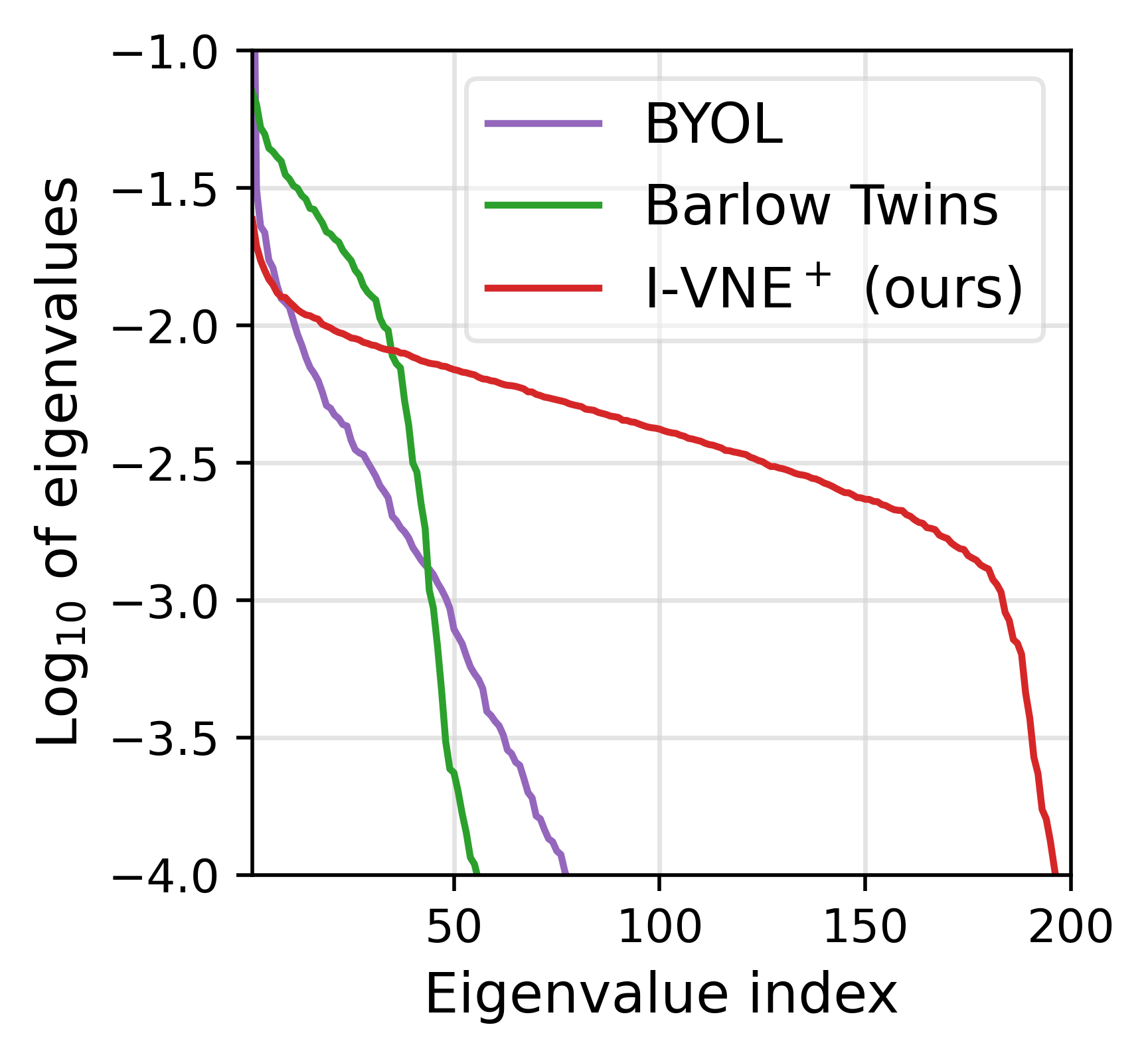
(a)

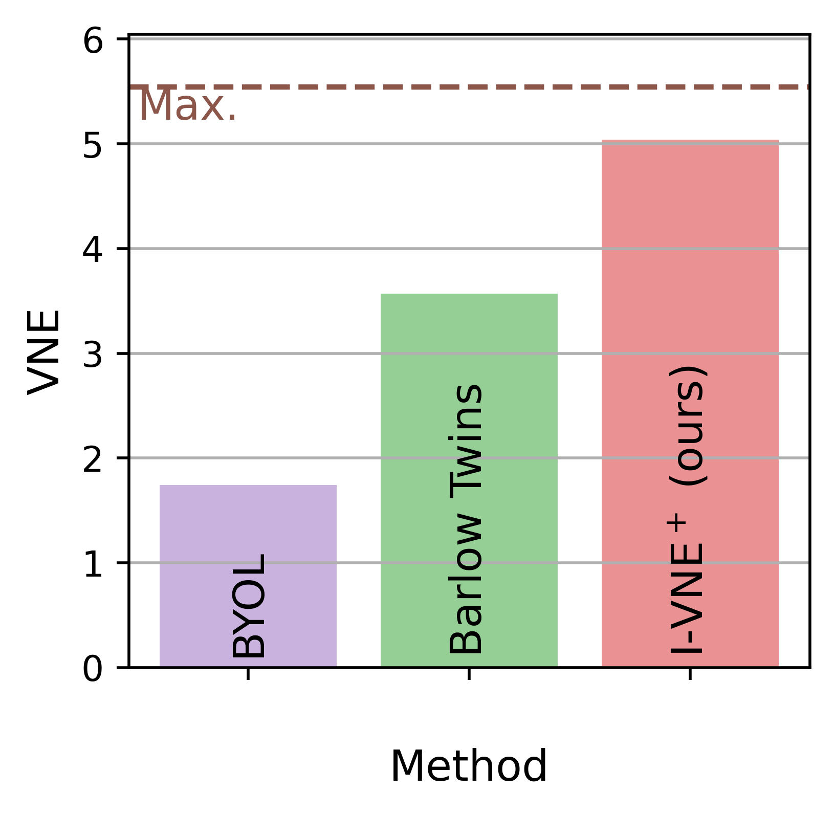
(b)

Figure 5: SSL: In (a), Eigenvalues of $\mathcal{C}_{\text{auto}}$ are presented in log₁₀ scale and descending order. In (b), von Neumann entropies are presented. ResNet-50 encoders and mlp projectors are trained by BYOL, Barlow Twins, and I-VNE⁺ methods with ImageNet-100 for 100 epochs. Projectors for all methods have the same output dimension of 256.

In fact, the loss formulation in Eq. (5) is equivalent to a simple combination of the loss term in BYOL [35] and VNE⁺ without predictor and stop gradient. $S(\mathcal{C}_{\text{auto}})$ term in I-VNE⁺ can also replace the redundancy reduction term in Barlow Twins [96]. Therefore, we have analyzed the eigenvalue distribution of $\mathcal{C}_{\text{auto}}$ and $S(\mathcal{C}_{\text{auto}})$ by comparing with BYOL and Barlow Twins, and the results are presented in Figure 5. Simply put, I-VNE⁺ utilizes more eigenvalues of $\mathcal{C}_{\text{auto}}$ and has a larger value of $S(\mathcal{C}_{\text{auto}})$ than the others. Because I-VNE⁺ utilizes more eigen-dimensions of $\mathcal{C}_{\text{auto}}$ than the others, the dimensional collapse problem prevailing in SSL [43, 47] can be mitigated by I-VNE⁺; hence better performance with I-VNE⁺ can be expected.

Method	Epoch	Top-1
Supervised [14]		95.1
NT-Xent [15]	200	91.3
Decoupled NT-Xent [15]	200	91.3
SWD [15]	200	90.8
NT-Xent [15]	800	93.9
Decoupled NT-Xent [15]	800	94.0
SWD [15]	800	94.1
Shuffled-DBN [43]	200	89.5
I-VNE+ (ours)	200	94.3
I-VNE+ (ours)	400	94.3

(a)

Method	Epoch	Top-1
Supervised [48]		86.2
Align.+Uniform. [87]	240	74.6
CMC (K=1) [97]	200	75.8
CMC (K=4) [97]	200	78.8
CACR(K=1) [97]	200	79.4
CACR(K=4) [97]	200	80.5
LooC++ [91]	500	82.2
MoCo-v2+MoCHi [48]	800	84.5
I-VNE+ (ours)	200	84.7
I-VNE+ (ours)	800	86.3

(b)

Table 5: SSL: Linear evaluation performance for various representation learning methods. They are all based on ResNet-50 encoders pre-trained with various datasets. Linear classifier on top of the frozen pre-trained model is trained with labels. State-of-the-art methods are included and the best results are indicated in bold.

To evaluate I-VNE⁺, we compare benchmark performance with prior state-of-the-art methods. In Table 5(a) and (b), I-VNE⁺ outperforms prior state-of-the-art linear evaluation benchmarks in both CIFAR-10 and ImageNet-100. Moreover, I-VNE⁺ even surpasses the supervised performance in ImageNet-100. In ImageNet-1K, I-VNE⁺ shows competitive linear evaluation performance which is above the average (71.8%) as demonstrated in Table 10 of Supplementary F. In addition, we can show that the pre-trained model of ImageNet-1K shows state-of-the-art performance in the following evaluation benchmarks. In Table 6, I-VNE⁺ outperforms all the semi-supervised learning benchmarks except for Top-1 accuracy with 10% data regime. In Table 7, I-VNE⁺ outperforms all the transfer learning benchmarks with COCO. The results indicate that I-VNE⁺ is advantageous for more sophisticated tasks such as low-data regime (semi-supervised) and out-of-domain (transfer learning with COCO) tasks.

Method	Top-1		Top-5
	1$\%$	10$\%$	1$\%$	10$\%$
Supervised [14]	25.4	56.4	48.4	80.4
SimCLR [14]	48.3	65.6	75.5	87.8
BYOL [35]	53.2	68.8	78.4	89.0
SwAV [11]	53.9	70.2	78.5	89.9
VICReg [7]	54.8	69.5	79.4	89.5
Barlow Twins [96]	55.0	69.7	79.2	89.3
I-VNE+ (ours)	55.8	69.1	81.0	89.9

Table 6: SSL: Semi-supervised learning evaluation performance for various representation learning methods. They are all based on ResNet-50 encoders pre-trained with ImageNet-1K. Pre-trained models are fine-tuned with 1% and 10% labels of ImageNet-1K. State-of-the-art methods are included and the best results are indicated in bold.

Method	COCO det.			COCO instance seg.
	AP	AP50	AP75	AP${}^{\text{mask}}$	AP${}_{50}^{\text{mask}}$	AP${}_{75}^{\text{mask}}$
Scratch [18]	26.4	44.0	27.8	29.3	46.9	30.8
Supervised [18]	38.2	58.2	41.2	33.3	54.7	35.2
SimCLR [18]	37.9	57.7	40.9	33.3	54.6	35.3
BYOL [18]	37.9	57.8	40.9	33.2	54.3	35.0
SwAV [96]	38.4	58.6	41.3	33.8	55.2	35.9
SimSiam [18]	39.2	59.3	42.1	34.4	56.0	36.7
MoCov2 [96]	39.3	58.9	42.5	34.4	55.8	36.5
Barlow Twins [96]	39.2	59.0	42.5	34.3	56.0	36.5
I-VNE+ (ours)	41.2	61.3	44.6	35.7	57.9	38.0

Table 7: SSL: Transfer learning evaluation performance for various representation learning methods. They are all based on ResNet-50 encoders pre-trained in ImageNet-1K. Pre-trained models are fine-tuned with COCO detection and instance segmentation tasks using Mask R-CNN with C4-backbone [37, 90] and using 1 $\times$ schedule. State-of-the-art methods are included and the best results are indicated in bold.

3.4 GAN: Preventing Mode Collapse

In Section 3.3, VNE⁺ has successfully prevented representation collapse. As another example for collapse prevention, we consider the mode collapse in GAN. The GAN training usually ends up with (partial) mode collapse [33], where generative models suffer lack of diversity. To demonstrate that this problem can be solved by VNE⁺, we reproduce various GAN methods based on an open source code base, StudioGAN [49] and train all models with CIFAR-10 for 100 epochs. To evaluate the models, we report the Inception Score [74] (IS, higher is better) and the Fréchet Inception Distance [40] (FID, lower is better). Although both IS and FID are the most popular metrics for evaluating generative models, FID is known to favor more diversified images [10]. Table 8 demonstrate that the overall quality of the output, especially diversity, has been improved by VNE⁺ because FID scores have been improved. IS has also been improved.

	Inception Score $\uparrow$			Fréchet Inception Distance $\downarrow$
Method	Vanilla	VNE+	Diff.	Vanilla	VNE+	Diff.
DCGAN	6.49	6.74	$\uparrow$ 0.25	42.55	35.44	$\downarrow$ 7.11
PD-GAN	7.83	8.01	$\uparrow$ 0.18	28.02	23.54	$\downarrow$ 4.48
LOGAN	8.02	8.15	$\uparrow$ 0.13	18.88	17.17	$\downarrow$ 1.71
WGAN-GP	7.37	7.42	$\uparrow$ 0.05	24.62	23.31	$\downarrow$ 1.31
SAGAN	8.86	8.90	$\uparrow$ 0.04	09.55	08.91	$\downarrow$ 0.64
SNGAN	8.85	8.86	$\uparrow$ 0.01	09.97	09.41	$\downarrow$ 0.56
BigGAN	9.82	9.83	$\uparrow$ 0.01	05.34	05.18	$\downarrow$ 0.16

Table 8: GAN: Performance evaluation results.

4 Theoretical Connections of VNE

In Section 2, we have examined the popular regularization objective of $\mathcal{C}_{\text{auto}}\rightarrow c\cdot I_{d}$ and explained how von Neumann entropy can be a desirable regularization method. In addition, von Neumann entropy can be beneficial in a few different ways because of its conceptual connection with conventional representation properties such as rank, disentanglement, and isotropy. In this section, we establish a theoretical connection with each property and provide a brief discussion.

4.1 Rank of Representation

The rank of representation, $\text{rank}(\mathcal{C}_{\text{auto}})$, directly measures the number of dimensions utilized by the representation. Von Neumann Entropy in Eq. (3) is closely related to the rank, where it is maximized when $\mathcal{C}_{\text{auto}}$ is full rank with uniformly distributed eigenvalues and it is minimized when $\mathcal{C}_{\text{auto}}$ is rank one. In fact, a formal bound between rank and VNE can be derived.

Theorem 1 (Rank and VNE).

For a given representation autocorrelation $\mathcal{C}_{\text{auto}}=\bm{H}^{T}\bm{H}/N\in\mathbb{R}^{d\times d}$ of rank $k$ $(\leq d)$,

$$\text{log}(\text{rank}(\mathcal{C}_{\text{auto}}))\geq S(\mathcal{C}_{\text{auto}}),$$ (6)

where equality holds iff the eigenvalues of $\mathcal{C}_{\text{auto}}$ are uniformly distributed with $\forall_{j=1}^{k}\lambda_{j}=1/k$ and $\forall_{j=k+1}^{d}\lambda_{j}=0$.

Refer to Supplementary B for the proof. Theorem 1 states that $\text{log}(\text{rank}(\mathcal{C}_{\text{auto}}))$ is lower bounded by $S(\mathcal{C}_{\text{auto}})$ and that the bound is tight when non-zero eigenvalues are uniformly distributed. The close relationship between rank and VNE can also be confirmed empirically. For the VNE plots in Figure 3(b) and Figure 4(b), we have compared their rank values and the results are presented in Figure 7.

Although the rank is a meaningful and useful measure of $\mathcal{C}_{\text{auto}}$, it cannot be directly used for learning because of its discrete nature. In addition, it can be misleading because even extremely small non-zero eigenvalues contribute toward the rank. VNE can be a useful proxy of the rank because it does not suffer from either of the problems.

(a)

(b)

Figure 7: Rank of representation: Comparison between $\text{log}(\text{rank}(\mathcal{C}_{\text{auto}}))$ and $S(\mathcal{C}_{\text{auto}})$. As a surrogate of the rank, the count of the largest eigenvalues required for the 99% of total eigenvalue energy is presented. The possible maximum value, $\log{d}$, is depicted as the brown dotted line.

4.2 Disentanglement of Representation

Although disentanglement has been considered as a desirable property of representation [9, 1], its formal definition can be dependent on the context of the research. In this study, we adopt the definition in [1], where a representation vector $\bm{h}$ is disentangled if its scalar components are independent. To understand the relationship between von Neumann entropy and disentanglement, we derive a theoretical result under a multi-variate Gaussian assumption and provide an empirical analysis. The assumption can be formally described as:

Assumption 1.

We assume that representation $\bm{h}$ follows zero-mean multivariate Gaussian distribution. In addition, we assume that the components of $\bm{h}$ (denoted as $\bm{h}^{(i)}$) have homogeneous variance of $\frac{1}{d}$, i.e., $\forall_{i=1}^{d}\bm{h}^{(i)}\sim\mathcal{N}(0,\frac{1}{d})$.

The multi-variate Gaussian assumption is not new, and it has been utilized in numerous studies. For instance, [52, 55, 95] adopted the assumption. In addition, the assumption was proven to be true for infinite width neural networks [65, 89, 66, 55]. Numerous studies applied a representation normalization to have a homogeneous variance (e.g., via batch normalization [46]). Under the Assumption 1, our main result can be stated as below.

Theorem 2 (Disentanglement and VNE).

Under the Assumption 1, $\bm{h}$ is disentangled if $S(\mathcal{C}_{\text{auto}})$ is maximized.

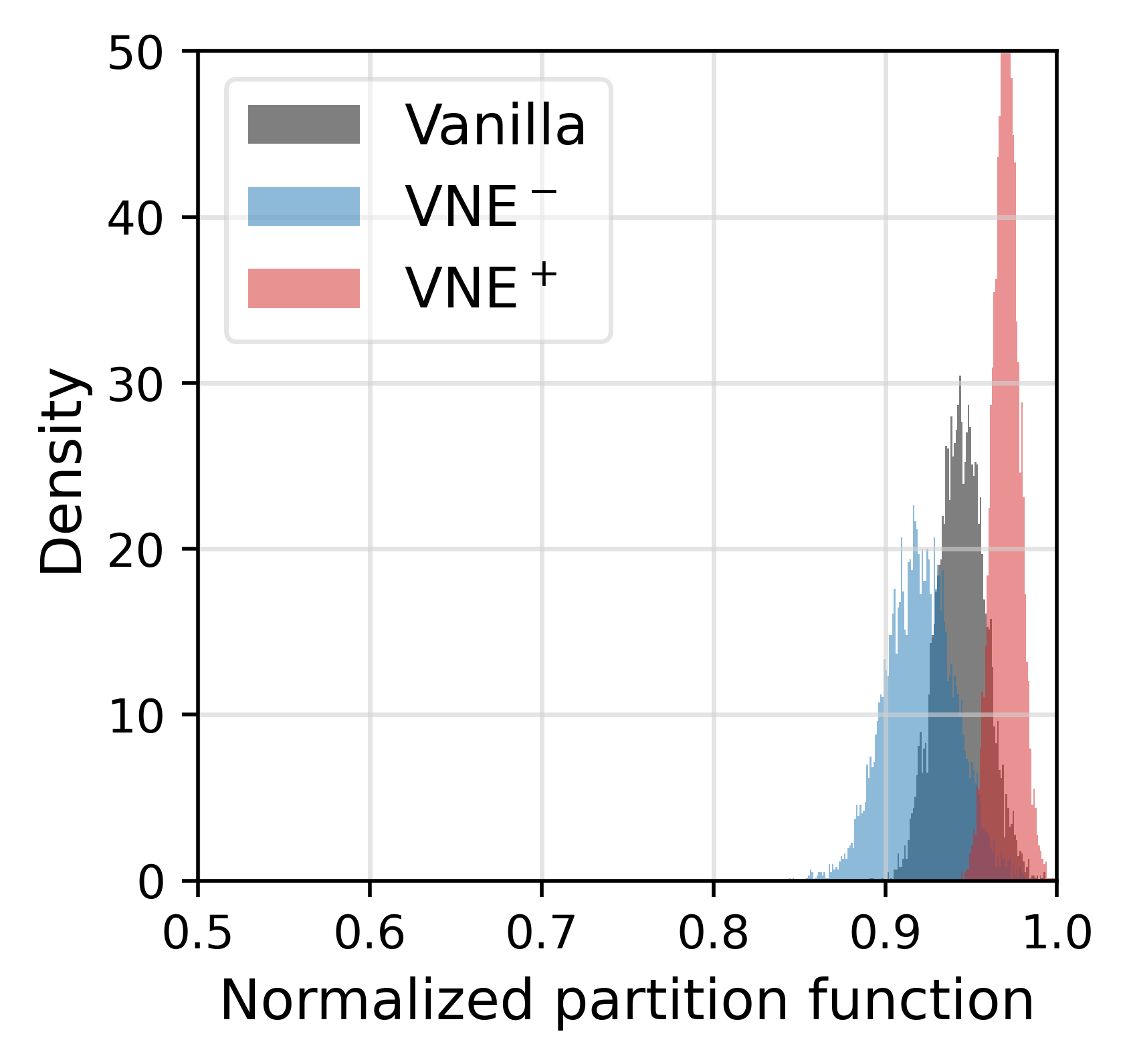
Figure 12: Domain generalization: Isotropy of representation.

Refer to Supplementary B for the proof. Theorem 2 states that the Gaussian representation $\bm{h}$ is disentangled if von Neumann entropy $S(\mathcal{C}_{\text{auto}})$ is fully maximized. The theoretical result can also be confirmed with an empirical analysis. For the domain-generalization experiment in Section 3, we have randomly chosen two components $\bm{h}^{(i)}$ and $\bm{h}^{(j)}$, where $i\neq j$, and compared their cosine similarity for the examples in the mini-batch. The resulting distributions are presented in Figure 8(a). It can be clearly observed that VNE⁺ makes the linear dependence between two components to be significantly weaker (cosine similarity closer to zero) while VNE^- can make it stronger. The same behavior can be observed for a supervised learning example in Figure 8(b). Therefore, the representation components are decorrelated by VNE⁺ and correlated by VNE^-. For meta-learning, the trend is the same, but the shift in the distribution turns out to be relatively limited (see Figure 12 in Supplementary F).

Similar to the case of rank, von Neumann entropy can be utilized as a proxy for controlling the degree of disentanglement in representation. In the case of supervised learning in Figure 8(b), it can be observed that both highly disentangled and highly entangled representations can be learned by regularizing von Neumann entropy.

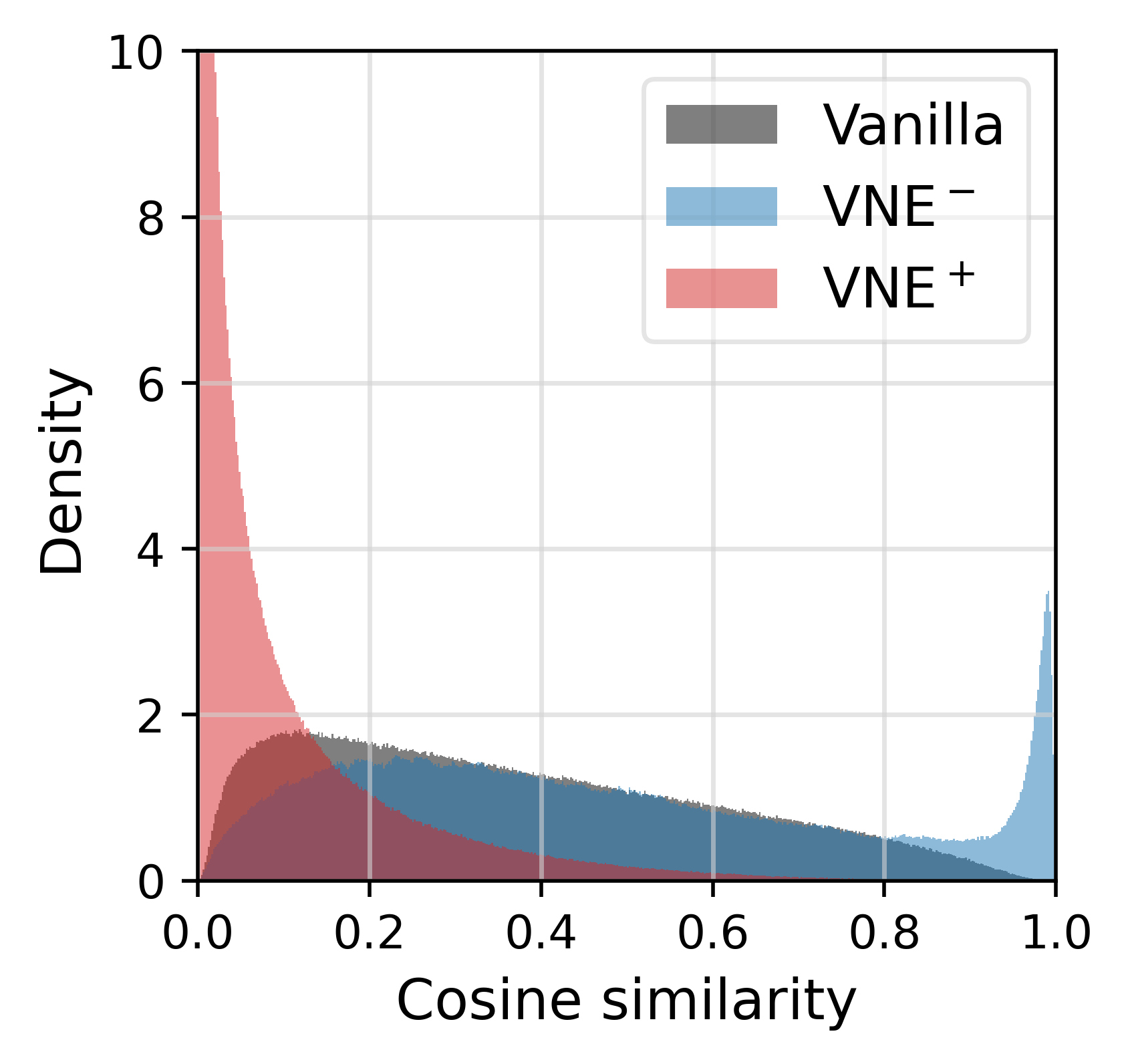
(a)

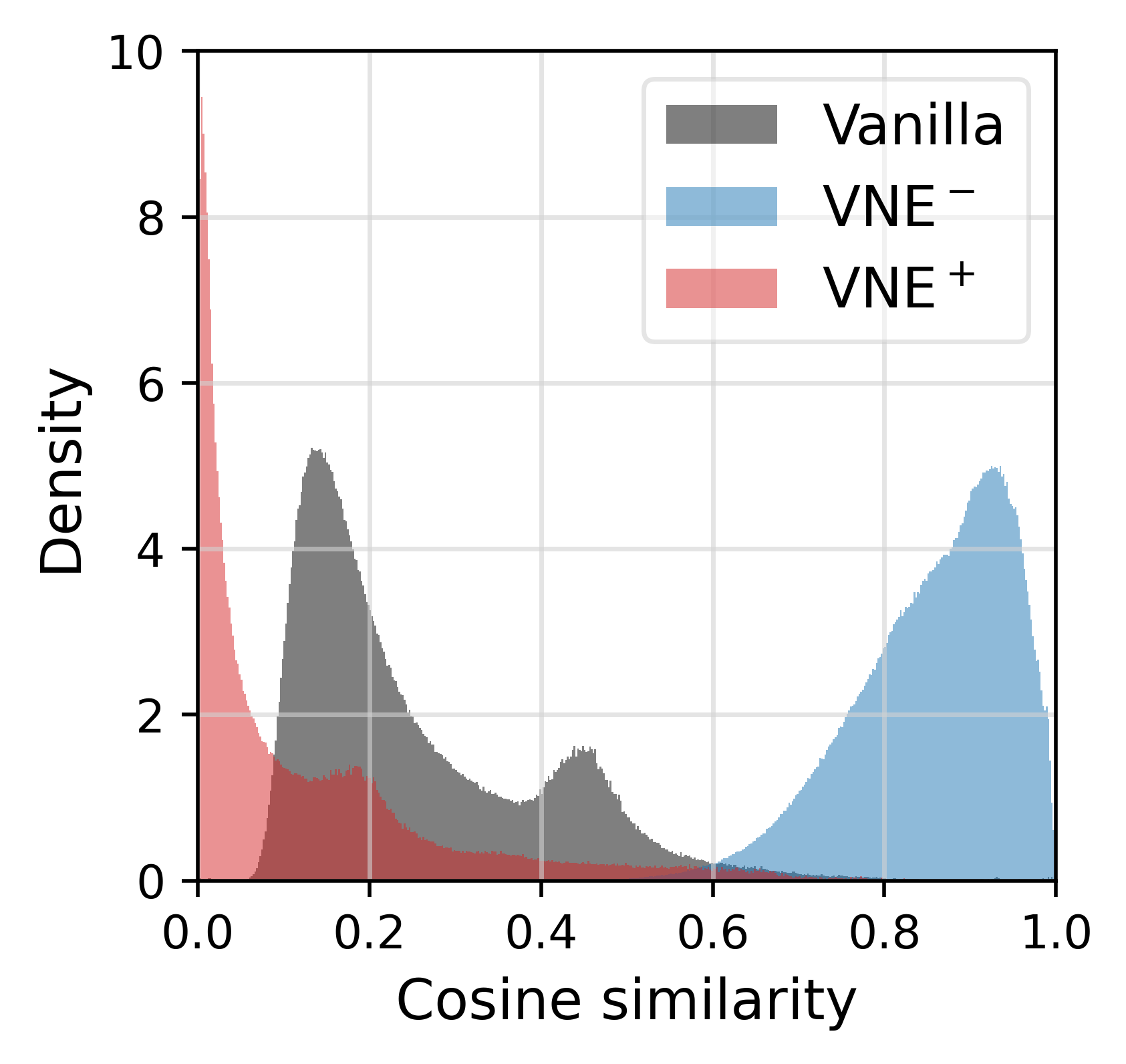
(b)

Figure 8: Disentanglement of representation: Distribution of cosine similarity between pairwise components in representation. Note that all the values are positive because of the ReLU layer.

4.3 Isotropy of Representation

The autocorrelation of representation is defined as $\mathcal{C}_{\text{auto}}=\bm{H}^{T}\bm{H}/N\in\mathbb{R}^{d\times d}$ where $d$ is the representation vector’s size. In contrast, isotropy concerns $\bm{H}\bm{H}^{T}\in\mathbb{R}^{N\times N}$ because it handles the uniformity in all orientations for the $N$ representation vectors in the $d$-dimensional vector space. Similar to the rank and disentanglement, we first provide a theoretical result.

Theorem 3 (Isotropy and VNE).

For a given representation matrix $\bm{H}\in\mathbb{R}^{N\times d}$, suppose that $N\leq d$ and $S(\mathcal{C}_{\text{auto}})$ is maximized. Then,

$$\bm{H}\bm{H}^{T}=\bm{I}_{N}.$$ (7)

Refer to Supplementary B for the proof. Theorem 3 states that if $S(\mathcal{C}_{\text{auto}})$ is maximized, representation vectors are uniformly distributed in all orientations and thus isotropic [5]. To perform an empirical analysis, we follow the studies of [5, 64] and adopt the partition function $Z(\bm{c})=\sum_{i=1}^{N}\text{exp}(\bm{c}^{T}\bm{h}_{i})$ defined for an arbitrary unit column vector $\bm{c}$. The partition function becomes constant when $\{\bm{h}_{1},\cdots,\bm{h}_{i},\cdots,\bm{h}_{N}\}$ are isotropically distributed. To be specific, the normalized partition function, $\frac{Z(\bm{c})}{\max_{||\bm{c}||=1}Z(\bm{c})}$, should become approximately 1 when the representation is isotropic (Lemma 2.1 in [5]). We have analyzed the normalized partition function for meta-learning and supervised learning, and the obtained results are presented in Figure 9. In both cases, it can be observed that isotropy is strengthened by VNE⁺ and weakened by VNE^-. For domain generalization, the trend is the same, but the shift in the distribution turns out to be relatively limited (see Figure 12 in Supplementary F). Based on the theoretical and empirical results, we can infer that the von Neumann entropy can be utilized as a proxy for controlling the representation’s isotropy.

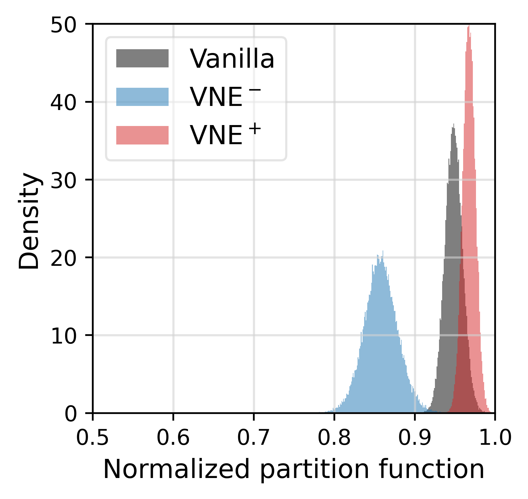
(a)

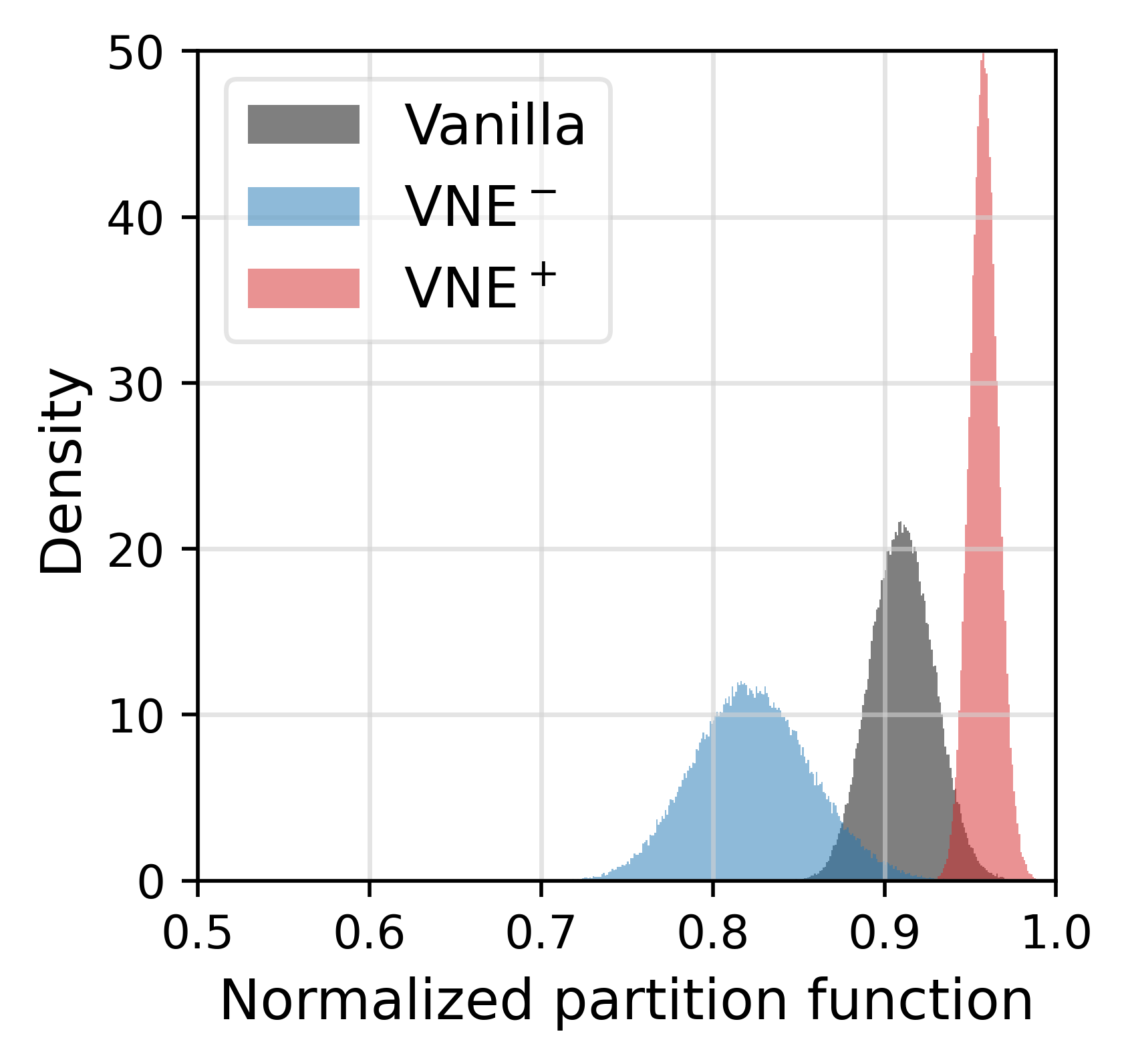
(b)

Figure 9: Isotropy of representation: Distribution of the normalized partition function values. Representation with its distribution closer to one is more isotropic.

5 Discussion

5.1 VNE and Dimension

Although a large amount of information can be contained in a representation, it is known that the usable information is intimately linked to the predictive models that have computational constraints [94, 25]. For instance, the representation decodability can be a critical factor when performing a linear evaluation [3]. From this perspective, decorrelation, disentanglement, whitening, and isotropy can be understood as improving decodability by encouraging a representation to use as many dimensions as possible with a full utilization of each dimension. Von Neumann entropy can be understood in the same way, except that its mathematical formulation is superior as explained in Section 2.

In this context, it looks logical that VNE⁺ is beneficial in improving the performance of meta-learning, SSL, and GAN. However, for domain generalization, VNE⁺ is harmful and VNE^- is helpful. DG differs from the other tasks because the model needs to be ready for the same label-set but unseen target domains. Fine-tuning to the target domain is not allowed, either. In this case, the model needs to be trained to be solely dependent on the invariant features and not on the spurious features [4, 2, 6, 54]. Because it is important to discard spurious features in DG, it makes sense that VNE^- can be beneficial in reducing the number of dimensions and thus reducing the amount of usable information. However, if a very strong VNE^- is applied, it can be harmful because even invariant features can be discarded.

5.2 Von Neumann Entropy vs. Shannon Entropy

Von Neumann entropy is defined over the representation autocorrelation $\mathcal{C}_{\text{auto}}$. For the representation $\bm{h}$ itself, Shannon entropy can be defined and it is relevant because it is also a metric of entropy. In fact, it can be proven that von Neumann entropy is a lower bound of Shannon entropy [67].

Owing to the connection, we have investigated if Shannon Entropy (SE) can replace von Neumann entropy and achieve a better performance. Unlike VNE, however, regularizing Shannon metric is known to be difficult [53, 30] and its implementation can be challenging. In our investigation, we have focused on the fact that Shannon entropy is equivalent to Shannon self-information (i.e., $H(\bm{h})=I(\bm{h};\bm{h})$ [21]) and that self-information can be evaluated using the latest variational mutual information estimators. In particular, we have chosen InfoNCE [69, 71] as the mutual information estimator and regularized the Shannon entropy. An exemplary result for domain generalization is presented in Table 11 of Supplementary F. From the result, it can be observed that Shannon entropy can also improve the performance of ERM and SWAD. However, the overall improvement is smaller where the average improvements are 1.43% and 0.79% for VNE and SE, respectively. We have performed a similar comparison for SSL and reached the same conclusion. Although Shannon entropy is closely related to von Neumann entropy, the difficulty in manipulating Shannon entropy appears to make it less useful.

6 Conclusion

In this study, we have proposed von Neumann entropy for manipulating the eigenvalue distribution of the representation’s autocorrelation matrix $\mathcal{C}_{\text{auto}}$. We have shown why its mathematical formulation can be advantageous when compared to the conventional approach of Frobenius norm. Then, we have demonstrated von Neumann entropy’s general applicability by empirically investigating four major learning tasks: DG, meta-learning, SSL, and GAN. Finally, we have established von Neumann entropy’s theoretical connection with the conventional properties of rank, disentanglement, and isotropy. Overall, we conclude that von Neumann entropy is an effective and useful representation property for improving task performance.

Supplementary materials for the paper
“VNE: An Effective Method for Improving Deep Representation
by Manipulating Eigenvalue Distribution”

Appendix A A Brief Introduction to Quantum Theory

A classic bit can be either 0 or 1. In quantum theory [67, 88], a qubit is a quantum extension of the classic bit, and it can be in state $\ket{0}$, state $\ket{1}$, or any linear combination (superposition state) of the two as $\ket{\psi}=a\ket{0}+b\ket{1}$, where $|a|^{2}+|b|^{2}=1$.

Dirac notation and basic concepts:

Dirac notation is used in quantum theory [24]. For a state $\ket{\psi}$, $\psi$ should be understood as the name or label of the state. Because linear algebra provides the mathematical foundation of quantum theory, vector notation is adopted. For instance, in the simple example of $\ket{\psi}=a\ket{0}+b\ket{1}$, $\ket{\psi}$ can be expressed as $\ket{\psi}=[a,b]^{T}$ where the interpretation should be state $\ket{\psi}$ can be 0 with probability $|a|^{2}$ and 1 with probability $|b|^{2}$ (therefore $|a|^{2}+|b|^{2}=1$). Here, the ket vector $\ket{\psi}$ is the Dirac notation for a column vector in a Hilbert space $\mathcal{H}$. To represent a row vector, the bra vector $\bra{\psi}$ is used, as in $\bra{\psi}=[a,b]$. An inner product or braket is represented as $\innerproduct{\psi}{\phi}$ and an outer product or ketbra is represented as $\outerproduct{\psi}{\phi}$.

A composite quantum state of $n$ qubits can be represented as a vector of size $2^{n}$ (e.g., a single-qubit state is represented as a vector of size two). For example, a quantum state of two separable single-qubit states can be represented as

$$\begin{split}\ket{\psi}\otimes\ket{\phi}&=\ket{\psi}\ket{\phi}=\ket{\psi\phi}\\ &=[a,b]^{T}\otimes[c,d]^{T}=[ac,ad,bc,bd]^{T}\end{split}\vspace{-0.1cm}$$ (8)

in which $\absolutevalue{ac}^{2},\absolutevalue{ad}^{2},\absolutevalue{bc}^{2},$ and $\absolutevalue{bd}^{2}$ represent the probability of $\ket{\psi\phi}$ being $\ket{00},\ket{01},\ket{10}$, and $\ket{11}$, respectively. In $d$-dimensional quantum system, a quantum state is on the unit hypersphere in a Hilbert space $\mathcal{H}$.

A state can be either pure or mixed. In the simple example, $\ket{0}=[1,0]^{T}$ and $\ket{1}=[0,1]^{T}$ form the computational basis states, and they are pure states. Any superposition of the two, $\ket{\psi}=a\ket{0}+b\ket{1}$, is also a pure state because it corresponds to a single vector with a probabilistic distribution over the basis states. By contrast, a mixed state is a probabilistic mixture of a set of pure states. Note that a pure state already has a probabilistic interpretation over the basis states and a mixed state has an additional level of probabilistic interpretation over a set of such pure states. In this case, we are considering a state that is not completely known but is an ensemble of pure states $\{\ket{\psi_{i}}\}$ with respective probabilities $\{p_{i}\}$. The full information of a mixed state cannot be represented as a vector, and the notion of the density operator (also called density matrix) is required.

Definition 1 (Density operator [67]).

A density operator is defined as below.

$$\rho\triangleq\sum_{i}p_{i}\outerproduct{\psi_{i}}{\psi_{i}}.\vspace{-0.2cm}$$ (9)

Density operator $\rho$ satisfies $\rho\geq 0$ and $tr(\rho)=1$. In addition, $\rho=\rho^{2}$ and $rank(\rho)=1$ are satisfied for pure states and $tr(\rho^{2})<1$ is satisfied for mixed states. The density operator provides a convenient way to describe the uncertainty or probability distribution of a quantum system. According to Gleason’s theorem [31], the probability of a state $\ket{\psi_{i}}$ in the system with $\rho$ is given by $tr(\rho\outerproduct{\psi_{i}}{\psi_{i}})$.

While quantum theory encompasses a broad scope of subjects, quantum information theory or quantum Shannon theory is a sub-field that focuses on the quantum equivalent of Shannon information theory [88]. Among the extensive results, we utilize the basic concepts of von Neumann entropy (also called quantum entropy). While Shannon entropy is calculated for a classical probability distribution, von Neumann entropy is calculated for a density operator $\rho$ [67], a positive semi-definite hermitian matrix in a Hilbert space $\mathcal{H}$ with the trace value of one. Similar to Shannon information theory, it measures the uncertainty associated with a quantum system.

Definition 2 (von Neumann entropy [67]).

The von Neumann entropy (quantum entropy) of a quantum state with density operator $\rho$ is defined as

$$S(\rho)\triangleq-tr(\rho\log{\rho})=-\sum_{j}\lambda_{j}\log{\lambda_{j}},\vspace{-0.2cm}$$ (10)

where {$\lambda_{j}$} are the eigenvalues of $\rho$.

Appendix B Proofs of Theorems

Lemma 1.

For given $p_{i}\geq 0$ and $\sum_{i=1}^{n}p_{i}=1$, the entropy function $H(p_{1},...,p_{n})=-\sum_{i=1}^{n}p_{i}\log{p_{i}}$ is strictly concave and is upper-bounded by $\log{n}$ as follows,

$$\log{n}=H(1/n,...,1/n)\geq H(p_{1},...,p_{n})\geq 0.\vspace{-0.2cm}$$ (11)

Proof.

Refer to Section D.1 in [61]. ∎

Lemma 2.

The KL Divergence for two zero-mean $d$-dimensional multivariate Gaussian distributions can be derived as follows,

$$\begin{split}&D_{\mathrm{KL}}(\mathcal{N}(0,\bm{\Sigma}_{1})\|\mathcal{N}(0,\bm{\Sigma}_{2}))\\ &=\frac{1}{2}\left[\text{tr}(\bm{\Sigma}_{2}^{-1}\bm{\Sigma}_{1})-d+\log\frac{|\bm{\Sigma}_{2}|}{|\bm{\Sigma}_{1}|}\right].\vspace{-0.2cm}\end{split}$$ (12)

Proof.

Refer to Section 9 in [26]. ∎

Theorem 1 (Rank and VNE).

For a given representation autocorrelation $\mathcal{C}_{\text{auto}}=\bm{H}^{T}\bm{H}/N\in\mathbb{R}^{d\times d}$ of rank $k$ $(\leq d)$,

$$\text{log}(\text{rank}(\mathcal{C}_{\text{auto}}))\geq S(\mathcal{C}_{\text{auto}}),$$ (13)

where equality holds iff the eigenvalues of $\mathcal{C}_{\text{auto}}$ are uniformly distributed with $\forall_{j=1}^{k}\lambda_{j}=1/k$ and $\forall_{j=k+1}^{d}\lambda_{j}=0$.

Proof.

$$\text{log}(\text{rank}(\mathcal{C}_{\text{auto}})) =\text{log}(k)$$ (14)

$$\geq H(\lambda_{1},...,\lambda_{k})\text{ (by Lemma~{}\ref{lem:entropy})}$$ (15)

$$=-\sum_{j=1}^{k}\lambda_{j}\log{\lambda_{j}}$$ (16)

$$=-\sum_{j=1}^{d}\lambda_{j}\log{\lambda_{j}}$$ (17)

$$=S(\mathcal{C}_{\text{auto}}).$$ (18)

By Lemma 1, the inequality (15) holds with equality if and only if $\forall_{j=1}^{k}\lambda_{j}=1/k$. The Eq. (17) follows from the convention $0\log{0}=0$ [21]. ∎

Assumption 1.

We assume that representation $\bm{h}$ follows zero-mean multivariate Gaussian distribution. In addition, we assume that the components of $\bm{h}$ (denoted as $\bm{h}^{(i)}$) have homogeneous variance of $\frac{1}{d}$, i.e., $\forall_{i=1}^{d}\bm{h}^{(i)}\sim\mathcal{N}(0,\frac{1}{d})$.

Theorem 2 (Disentanglement and VNE).

Under the Assumption 1, $\bm{h}$ is disentangled if $S(\mathcal{C}_{\text{auto}})$ is maximized.

Proof.

By Assumption 1, $\bm{h}\sim\mathcal{N}(0,\bm{\Sigma}_{1})$ for $\bm{\Sigma}_{1}\in\mathbb{R}^{d\times d}$ where diagonal entries in $\bm{\Sigma}_{1}$ are equal to $1/d$.

In addition, we define new random variable $\bm{h}^{\prime}\sim\mathcal{N}(0,\bm{\Sigma}_{2})$ for $\bm{\Sigma}_{2}=\frac{1}{d}\cdot I_{d}$.

Then, because $\bm{h}^{(i)}\sim\mathcal{N}(0,\frac{1}{d})$ and $\bm{h}^{\prime(i)}\sim\mathcal{N}(0,\frac{1}{d})$ and the components of $\bm{h}^{\prime}$ are independent,

$$\prod_{i=1}^{d}p(\bm{h}^{(i)})=\prod_{i=1}^{d}p(\bm{h}^{\prime(i)})=p(\bm{h}^{\prime}).\vspace{-0.1cm}$$ (19)

By Lemma 1, $S(\mathcal{C}_{\text{auto}})$ is maximized if and only if

$$\forall_{j=1}^{d}\lambda_{j}=\frac{1}{d},\vspace{-0.1cm}$$ (20)

where $\lambda_{j}$ are eigenvalues of $\bm{\Sigma}_{1}(=\mathbb{E}[\bm{h}\bm{h}^{T}]=\mathcal{C}_{\text{auto}})$.

Starting from Definition of total correlation $TC(\bm{h})$ in [1], we have

$$2\cdot TC(\bm{h}) =2\cdot D_{\mathrm{KL}}(p(\bm{h})\|\prod_{i=1}^{d}p(\bm{h}^{(i)}))$$ (21)

$$=2\cdot D_{\mathrm{KL}}(p(\bm{h})\|p(\bm{h}^{\prime}))$$ (22)

$$=\text{tr}(\bm{\Sigma}_{2}^{-1}\bm{\Sigma}_{1})-d+\log{\frac{|\bm{\Sigma}_{2}|}{|\bm{\Sigma}_{1}|}}$$ (23)

$$=d-d+\log{\frac{(1/d)^{d}}{(1/d)^{d}}}=0,$$ (24)

where Eq. (22) follows from Eq. (19), Eq. (23) follows from Lemma 2, and Eq. (24) follows from Eq. (20).

If $TC(\bm{h})=0$, the components of $\bm{h}$ are independent, therefore $\bm{h}$ is disentangled [1]. ∎

Theorem 3 (Isotropy and VNE).

For a given representation matrix $\bm{H}\in\mathbb{R}^{N\times d}$, suppose that $N\leq d$ and $S(\mathcal{C}_{\text{auto}})$ is maximized. Then,

$$\bm{H}\bm{H}^{T}=\bm{I}_{N}.\vspace{-0.1cm}$$ (25)

Proof.

We consider singular value decomposition of $\bm{H}(=\bm{U}\bm{\Sigma}\bm{V}^{T})$ for $\bm{U}\in\mathbb{R}^{N\times N}$, $\bm{\Sigma}\in\mathbb{R}^{N\times d}$, and $\bm{V}\in\mathbb{R}^{d\times d}$. If $N\leq d$ and $S(\mathcal{C}_{\text{auto}})$ is maximized, by Lemma 1, eigenvalues of $\mathcal{C}_{\text{auto}}(=\bm{H}^{T}\bm{H}/N=\bm{V}\bm{\Sigma}^{T}\bm{\Sigma}\bm{V}^{T}/N)$ are supposed to be equal to $1/N$ for the first $N$ eigenvalues and zero for the others. Therefore $\bm{\Sigma}\bm{\Sigma}^{T}=\bm{I}_{N}$ and we have

$$\bm{H}\bm{H}^{T}=\bm{U}\bm{\Sigma}\bm{\Sigma}^{T}\bm{U}^{T}=\bm{I}_{N}.\vspace{-0.1cm}$$ (26)

∎

Appendix C Main Algorithm

⬇

# N : batch size

# d : embedding dimension

# H : embeddings, Tensor, shape=[N, d]

\pardef get_vne(H):

Z = torch.nn.functional.normalize(H, dim=1)

rho = torch.matmul(Z.T, Z) / Z.shape[0]

eig_val = torch.linalg.eigh(rho)[0][-Z.shape[0]:]

return - (eig_val * torch.log(eig_val)).nansum()

\par# the following is equivalent and faster when N < d

def get_vne(H):

Z = torch.nn.functional.normalize(H, dim=1)

sing_val = torch.svd(Z / np.sqrt(Z.shape[0]))[1]

eig_val = sing_val ** 2

return - (eig_val * torch.log(eig_val)).nansum()

Figure 10: PyTorch implementation of VNE.

Appendix D Computational Overhead

We train I-VNE⁺ using 2$\times$RTX 3090 GPUs, ImageNet-1K, and various batch sizes and models. In Table 9, the average computational overhead is 2.68%.

Model		ResNet-18			ResNet-50
Batch Size		256	128	64	256	128	64
Average training time	On VNE	0.051	0.024	0.011	0.120	0.073	0.031
per iteration (sec.)	Total	2.318	1.288	0.845	2.745	2.101	1.127
Overhead		2.21%	1.89%	1.36%	4.37%	3.48%	2.75%

Table 9: Computational overhead of VNE.

Appendix E Experimental Details for I-VNE⁺

The PyTorch implementation codes will be made available online. Our implementations follow the standard training protocols of SSL in [35, 96] and the standard evaluation protocols of SSL in [63, 34, 35, 96]. A few important hyperparameters are described as follows.

Backbone and Projector: For all datasets, we use ResNet-50 [38] as the default backbone. For CIFAR-10, we use 2-layer MLP projector with hidden dimension of 2048 and output dimension of 128. For ImageNet-100, we use 3-layer MLP projector with hidden dimension of 2048 and output dimension of 256. For ImageNet-1K, we use the same projector as in the ImageNet-100 case, except that the output dimension is 512.

Optimization: We use SGD optimizer with momentum of 0.9. The learning rate (LR) is linearly scaled with batch size (LR = base learning rate $\times$ batch size / 256), and it is scheduled by the cosine learning rate decay with 10-epoch warm-up [59]. For CIFAR-10 and ImageNet-100, we use base learning rate of 0.4, batch size of 64, and weight decay of 1e-4. For ImageNet-1K, we use base learning rate of 0.2, batch size of 512, and weight decay of 1e-5.

Augmentation: For CIFAR-10 and ImageNet-100, we adopt multi-view setting in [11] and generate 6 views using the same augmentations in [14] (for CIFAR-10) and in [11] (for ImageNet-100). For ImageNet-1K, we generate the default 2 views using the same augmentation as in [35]. Note that we use 2-view setting for ImageNet-1K because of the computational limitation.

Appendix F Supplementary Results

Method	Top-1	Top-5
Supervised [14]	76.5	93.7
SimCLR [14]	69.3	89.0
MoCo v2 [17]	71.1	90.1
InfoMin Aug. [81]	73.0	91.1
BYOL [35]	74.3	91.6
SwAV [11]	75.3
Shuffled-DBN [43]	65.2
Barlow Twins [96]	73.2	91.0
VICReg [7]	73.2	91.1
I-VNE+ (ours)	72.1	91.0

Table 10: SSL: Linear evaluation performance in ImageNet-1K for various representation learning methods. They are all based on ResNet-50 encoders pre-trained with various datasets. Linear classifier on top of the frozen pre-trained model is trained with labels. State-of-the-art methods are included and the best results are indicated in bold.

0

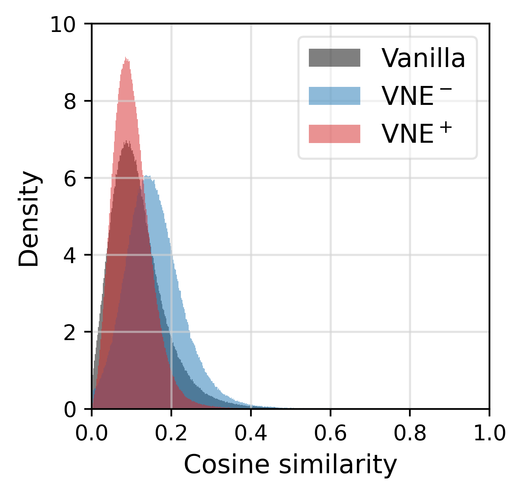
Figure 11: Meta-learning: Disentanglement of representation.

0

Algorithm	Method	PACS		VLSC		OfficeHome		TerraIncognita
		Avg.	Diff.	Avg.	Diff.	Avg.	Diff.	Avg.	Diff.
ERM	Vanilla	85.2		76.7		64.9		45.4
	VNE-	86.9	1.7	78.1	1.4	65.9	1.0	50.6	5.2
	SE-	85.0	-0.2	76.5	-0.2	65.3	0.4	50.4	5.0
SWAD	Vanilla	88.2		79.4		70.2		50.9
	VNE-	88.3	0.1	79.7	0.3	71.1	0.9	51.7	0.8
	SE-	88.4	0.2	79.6	0.1	71.0	0.8	51.2	0.2

Table 11: Von Neumann entropy vs. Shannon entropy: The results of domain generalization with ERM and SWAD algorithms are shown. For regularizing Shannon entropy, we have used the InfoNCE estimation of self-information, $I_{\text{NCE}}(\bm{h};\bm{h})$.

References

- [1] Alessandro Achille and Stefano Soatto. Emergence of invariance and disentanglement in deep representations. The Journal of Machine Learning Research, 19(1):1947–1980, 2018.
- [2] Kartik Ahuja, Ethan Caballero, Dinghuai Zhang, Jean-Christophe Gagnon-Audet, Yoshua Bengio, Ioannis Mitliagkas, and Irina Rish. Invariance principle meets information bottleneck for out-of-distribution generalization. Advances in Neural Information Processing Systems, 34:3438–3450, 2021.
- [3] Guillaume Alain and Yoshua Bengio. Understanding intermediate layers using linear classifier probes. arXiv preprint arXiv:1610.01644, 2016.
- [4] Martin Arjovsky, Léon Bottou, Ishaan Gulrajani, and David Lopez-Paz. Invariant risk minimization. arXiv preprint arXiv:1907.02893, 2019.
- [5] Sanjeev Arora, Yuanzhi Li, Yingyu Liang, Tengyu Ma, and Andrej Risteski. A latent variable model approach to pmi-based word embeddings. arXiv preprint arXiv:1502.03520, 2015.
- [6] Benjamin Aubin, Agnieszka Słowik, Martin Arjovsky, Leon Bottou, and David Lopez-Paz. Linear unit-tests for invariance discovery. arXiv preprint arXiv:2102.10867, 2021.
- [7] Adrien Bardes, Jean Ponce, and Yann LeCun. Vicreg: Variance-invariance-covariance regularization for self-supervised learning. arXiv preprint arXiv:2105.04906, 2021.
- [8] Sara Beery, Grant Van Horn, and Pietro Perona. Recognition in terra incognita. In Proceedings of the European conference on computer vision (ECCV), pages 456–473, 2018.
- [9] Yoshua Bengio et al. Learning deep architectures for ai. Foundations and trends® in Machine Learning, 2(1):1–127, 2009.
- [10] Andrew Brock, Jeff Donahue, and Karen Simonyan. Large scale gan training for high fidelity natural image synthesis. arXiv preprint arXiv:1809.11096, 2018.
- [11] Mathilde Caron, Ishan Misra, Julien Mairal, Priya Goyal, Piotr Bojanowski, and Armand Joulin. Unsupervised learning of visual features by contrasting cluster assignments. Advances in Neural Information Processing Systems, 33, 2020.
- [12] Junbum Cha, Sanghyuk Chun, Kyungjae Lee, Han-Cheol Cho, Seunghyun Park, Yunsung Lee, and Sungrae Park. Swad: Domain generalization by seeking flat minima. Advances in Neural Information Processing Systems, 34:22405–22418, 2021.
- [13] Ricky TQ Chen, Xuechen Li, Roger B Grosse, and David K Duvenaud. Isolating sources of disentanglement in variational autoencoders. Advances in neural information processing systems, 31, 2018.
- [14] Ting Chen, Simon Kornblith, Mohammad Norouzi, and Geoffrey Hinton. A simple framework for contrastive learning of visual representations. arXiv preprint arXiv:2002.05709, 2020.
- [15] Ting Chen, Calvin Luo, and Lala Li. Intriguing properties of contrastive losses. Advances in Neural Information Processing Systems, 34, 2021.
- [16] Wei-Yu Chen, Yen-Cheng Liu, Zsolt Kira, Yu-Chiang Frank Wang, and Jia-Bin Huang. A closer look at few-shot classification. arXiv preprint arXiv:1904.04232, 2019.
- [17] Xinlei Chen, Haoqi Fan, Ross Girshick, and Kaiming He. Improved baselines with momentum contrastive learning. arXiv preprint arXiv:2003.04297, 2020.
- [18] Xinlei Chen and Kaiming He. Exploring simple siamese representation learning. In Proceedings of the IEEE/CVF Conference on Computer Vision and Pattern Recognition, pages 15750–15758, 2021.
- [19] Daeyoung Choi and Wonjong Rhee. Utilizing class information for deep network representation shaping. In Proceedings of the AAAI Conference on Artificial Intelligence, volume 33, pages 3396–3403, 2019.
- [20] Michael Cogswell, Faruk Ahmed, Ross Girshick, Larry Zitnick, and Dhruv Batra. Reducing overfitting in deep networks by decorrelating representations. arXiv preprint arXiv:1511.06068, 2015.
- [21] Thomas M Cover. Elements of information theory. John Wiley & Sons, 1999.
- [22] Tristan Deleu, Tobias Würfl, Mandana Samiei, Joseph Paul Cohen, and Yoshua Bengio. Torchmeta: A meta-learning library for pytorch. arXiv preprint arXiv:1909.06576, 2019.
- [23] Guillaume Desjardins, Karen Simonyan, Razvan Pascanu, et al. Natural neural networks. Advances in neural information processing systems, 28, 2015.
- [24] Paul Adrien Maurice Dirac. A new notation for quantum mechanics. In Mathematical Proceedings of the Cambridge Philosophical Society, volume 35, pages 416–418. Cambridge University Press, 1939.
- [25] Yann Dubois, Douwe Kiela, David J Schwab, and Ramakrishna Vedantam. Learning optimal representations with the decodable information bottleneck. Advances in Neural Information Processing Systems, 33:18674–18690, 2020.
- [26] John Duchi. Derivations for linear algebra and optimization. Berkeley, California, 3(1):2325–5870, 2007.
- [27] Cian Eastwood and Christopher KI Williams. A framework for the quantitative evaluation of disentangled representations. In International Conference on Learning Representations, 2018.
- [28] Chen Fang, Ye Xu, and Daniel N Rockmore. Unbiased metric learning: On the utilization of multiple datasets and web images for softening bias. In Proceedings of the IEEE International Conference on Computer Vision, pages 1657–1664, 2013.
- [29] Chelsea Finn, Pieter Abbeel, and Sergey Levine. Model-agnostic meta-learning for fast adaptation of deep networks. In International conference on machine learning, pages 1126–1135. PMLR, 2017.
- [30] Shuyang Gao, Greg Ver Steeg, and Aram Galstyan. Efficient estimation of mutual information for strongly dependent variables. In Artificial intelligence and statistics, pages 277–286. PMLR, 2015.
- [31] Andrew M Gleason. Measures on the closed subspaces of a hilbert space. Journal of mathematics and mechanics, pages 885–893, 1957.
- [32] Xavier Glorot, Antoine Bordes, and Yoshua Bengio. Domain adaptation for large-scale sentiment classification: A deep learning approach. In ICML, 2011.
- [33] Ian Goodfellow. Nips 2016 tutorial: Generative adversarial networks. arXiv preprint arXiv:1701.00160, 2016.
- [34] Priya Goyal, Dhruv Mahajan, Abhinav Gupta, and Ishan Misra. Scaling and benchmarking self-supervised visual representation learning. In Proceedings of the IEEE/CVF International Conference on Computer Vision, pages 6391–6400, 2019.
- [35] Jean-Bastien Grill, Florian Strub, Florent Altché, Corentin Tallec, Pierre H Richemond, Elena Buchatskaya, Carl Doersch, Bernardo Avila Pires, Zhaohan Daniel Guo, Mohammad Gheshlaghi Azar, et al. Bootstrap your own latent: A new approach to self-supervised learning. arXiv preprint arXiv:2006.07733, 2020.
- [36] Ishaan Gulrajani and David Lopez-Paz. In search of lost domain generalization. arXiv preprint arXiv:2007.01434, 2020.
- [37] Kaiming He, Georgia Gkioxari, Piotr Dollár, and Ross Girshick. Mask r-cnn. In Proceedings of the IEEE international conference on computer vision, pages 2961–2969, 2017.
- [38] Kaiming He, Xiangyu Zhang, Shaoqing Ren, and Jian Sun. Deep residual learning for image recognition. In Proceedings of the IEEE conference on computer vision and pattern recognition, pages 770–778, 2016.
- [39] Olivier Henaff, Aravind Srinivas, Jeffrey De Fauw, Ali Razavi, Carl Doersch, Ali Eslami, and Aaron Van Den Oord. Data-efficient image recognition with contrastive predictive coding. In International Conference on Machine Learning, pages 4182–4192. PMLR, 2020.
- [40] Martin Heusel, Hubert Ramsauer, Thomas Unterthiner, Bernhard Nessler, and Sepp Hochreiter. Gans trained by a two time-scale update rule converge to a local nash equilibrium. Advances in neural information processing systems, 30, 2017.
- [41] Irina Higgins, Loic Matthey, Arka Pal, Christopher Burgess, Xavier Glorot, Matthew Botvinick, Shakir Mohamed, and Alexander Lerchner. beta-vae: Learning basic visual concepts with a constrained variational framework. In International conference on learning representations, 2017.
- [42] R Devon Hjelm, Alex Fedorov, Samuel Lavoie-Marchildon, Karan Grewal, Phil Bachman, Adam Trischler, and Yoshua Bengio. Learning deep representations by mutual information estimation and maximization. arXiv preprint arXiv:1808.06670, 2018.
- [43] Tianyu Hua, Wenxiao Wang, Zihui Xue, Sucheng Ren, Yue Wang, and Hang Zhao. On feature decorrelation in self-supervised learning. In Proceedings of the IEEE/CVF International Conference on Computer Vision, pages 9598–9608, 2021.
- [44] Lei Huang, Dawei Yang, Bo Lang, and Jia Deng. Decorrelated batch normalization. In Proceedings of the IEEE Conference on Computer Vision and Pattern Recognition, pages 791–800, 2018.
- [45] Lei Huang, Yi Zhou, Fan Zhu, Li Liu, and Ling Shao. Iterative normalization: Beyond standardization towards efficient whitening. In Proceedings of the IEEE/CVF Conference on Computer Vision and Pattern Recognition, pages 4874–4883, 2019.
- [46] Sergey Ioffe and Christian Szegedy. Batch normalization: Accelerating deep network training by reducing internal covariate shift. In International conference on machine learning, pages 448–456. PMLR, 2015.
- [47] Li Jing, Pascal Vincent, Yann LeCun, and Yuandong Tian. Understanding dimensional collapse in contrastive self-supervised learning. arXiv preprint arXiv:2110.09348, 2021.
- [48] Yannis Kalantidis, Mert Bulent Sariyildiz, Noe Pion, Philippe Weinzaepfel, and Diane Larlus. Hard negative mixing for contrastive learning. Advances in Neural Information Processing Systems, 33:21798–21809, 2020.
- [49] MinGuk Kang, Joonghyuk Shin, and Jaesik Park. StudioGAN: A Taxonomy and Benchmark of GANs for Image Synthesis. 2206.09479 (arXiv), 2022.
- [50] Tero Karras, Samuli Laine, and Timo Aila. A style-based generator architecture for generative adversarial networks. In Proceedings of the IEEE/CVF conference on computer vision and pattern recognition, pages 4401–4410, 2019.
- [51] Hyunjik Kim and Andriy Mnih. Disentangling by factorising. In International Conference on Machine Learning, pages 2649–2658. PMLR, 2018.
- [52] Diederik P Kingma and Max Welling. Auto-encoding variational bayes. arXiv preprint arXiv:1312.6114, 2013.
- [53] Alexander Kraskov, Harald Stögbauer, and Peter Grassberger. Estimating mutual information. Physical review E, 69(6):066138, 2004.
- [54] David Krueger, Ethan Caballero, Joern-Henrik Jacobsen, Amy Zhang, Jonathan Binas, Dinghuai Zhang, Remi Le Priol, and Aaron Courville. Out-of-distribution generalization via risk extrapolation (rex). In International Conference on Machine Learning, pages 5815–5826. PMLR, 2021.
- [55] Jaehoon Lee, Yasaman Bahri, Roman Novak, Samuel S Schoenholz, Jeffrey Pennington, and Jascha Sohl-Dickstein. Deep neural networks as gaussian processes. arXiv preprint arXiv:1711.00165, 2017.
- [56] Bohan Li, Hao Zhou, Junxian He, Mingxuan Wang, Yiming Yang, and Lei Li. On the sentence embeddings from pre-trained language models. arXiv preprint arXiv:2011.05864, 2020.
- [57] Da Li, Yongxin Yang, Yi-Zhe Song, and Timothy M Hospedales. Deeper, broader and artier domain generalization. In Proceedings of the IEEE international conference on computer vision, pages 5542–5550, 2017.
- [58] Weiyang Liu, Yandong Wen, Zhiding Yu, Ming Li, Bhiksha Raj, and Le Song. Sphereface: Deep hypersphere embedding for face recognition. In Proceedings of the IEEE conference on computer vision and pattern recognition, pages 212–220, 2017.
- [59] Ilya Loshchilov and Frank Hutter. Sgdr: Stochastic gradient descent with warm restarts. arXiv preprint arXiv:1608.03983, 2016.
- [60] Ping Luo. Learning deep architectures via generalized whitened neural networks. In International Conference on Machine Learning, pages 2238–2246. PMLR, 2017.
- [61] Albert W Marshall, Ingram Olkin, and Barry C Arnold. Inequalities: theory of majorization and its applications, volume 143. Springer, 1979.
- [62] Pascal Mettes, Elise van der Pol, and Cees Snoek. Hyperspherical prototype networks. Advances in neural information processing systems, 32, 2019.
- [63] Ishan Misra and Laurens van der Maaten. Self-supervised learning of pretext-invariant representations. In Proceedings of the IEEE/CVF Conference on Computer Vision and Pattern Recognition, pages 6707–6717, 2020.
- [64] Jiaqi Mu, Suma Bhat, and Pramod Viswanath. All-but-the-top: Simple and effective postprocessing for word representations. arXiv preprint arXiv:1702.01417, 2017.
- [65] Radford M Neal. Priors for infinite networks. In Bayesian Learning for Neural Networks, pages 29–53. Springer, 1996.
- [66] Radford M Neal. Bayesian learning for neural networks, volume 118. Springer Science & Business Media, 2012.
- [67] Michael A Nielsen and Isaac Chuang. Quantum computation and quantum information, 2002.
- [68] Jaehoon Oh, Hyungjun Yoo, ChangHwan Kim, and Se-Young Yun. Boil: Towards representation change for few-shot learning. arXiv preprint arXiv:2008.08882, 2020.
- [69] Aaron van den Oord, Yazhe Li, and Oriol Vinyals. Representation learning with contrastive predictive coding. arXiv preprint arXiv:1807.03748, 2018.
- [70] Omkar M Parkhi, Andrea Vedaldi, and Andrew Zisserman. Deep face recognition. 2015.
- [71] Ben Poole, Sherjil Ozair, Aaron Van Den Oord, Alex Alemi, and George Tucker. On variational bounds of mutual information. In International Conference on Machine Learning, pages 5171–5180. PMLR, 2019.
- [72] Aniruddh Raghu, Maithra Raghu, Samy Bengio, and Oriol Vinyals. Rapid learning or feature reuse? towards understanding the effectiveness of maml. arXiv preprint arXiv:1909.09157, 2019.
- [73] Subhankar Roy, Aliaksandr Siarohin, Enver Sangineto, Samuel Rota Bulo, Nicu Sebe, and Elisa Ricci. Unsupervised domain adaptation using feature-whitening and consensus loss. In Proceedings of the IEEE/CVF Conference on Computer Vision and Pattern Recognition, pages 9471–9480, 2019.
- [74] Tim Salimans, Ian Goodfellow, Wojciech Zaremba, Vicki Cheung, Alec Radford, and Xi Chen. Improved techniques for training gans. Advances in neural information processing systems, 29, 2016.
- [75] Florian Schroff, Dmitry Kalenichenko, and James Philbin. Facenet: A unified embedding for face recognition and clustering. In Proceedings of the IEEE conference on computer vision and pattern recognition, pages 815–823, 2015.
- [76] Aliaksandr Siarohin, Enver Sangineto, and Nicu Sebe. Whitening and coloring batch transform for gans. arXiv preprint arXiv:1806.00420, 2018.
- [77] Jake Snell, Kevin Swersky, and Richard Zemel. Prototypical networks for few-shot learning. Advances in neural information processing systems, 30, 2017.
- [78] Jianlin Su, Jiarun Cao, Weijie Liu, and Yangyiwen Ou. Whitening sentence representations for better semantics and faster retrieval. arXiv preprint arXiv:2103.15316, 2021.
- [79] Yaling Tao, Kentaro Takagi, and Kouta Nakata. Clustering-friendly representation learning via instance discrimination and feature decorrelation. arXiv preprint arXiv:2106.00131, 2021.
- [80] Yonglong Tian, Dilip Krishnan, and Phillip Isola. Contrastive multiview coding. In European conference on computer vision, pages 776–794. Springer, 2020.
- [81] Yonglong Tian, Chen Sun, Ben Poole, Dilip Krishnan, Cordelia Schmid, and Phillip Isola. What makes for good views for contrastive learning? Advances in Neural Information Processing Systems, 33:6827–6839, 2020.
- [82] Michael Tschannen, Josip Djolonga, Paul K Rubenstein, Sylvain Gelly, and Mario Lucic. On mutual information maximization for representation learning. arXiv preprint arXiv:1907.13625, 2019.
- [83] Hemanth Venkateswara, Jose Eusebio, Shayok Chakraborty, and Sethuraman Panchanathan. Deep hashing network for unsupervised domain adaptation. In Proceedings of the IEEE conference on computer vision and pattern recognition, pages 5018–5027, 2017.
- [84] Roman Vershynin. High-dimensional probability: An introduction with applications in data science, volume 47. Cambridge university press, 2018.
- [85] Oriol Vinyals, Charles Blundell, Timothy Lillicrap, Daan Wierstra, et al. Matching networks for one shot learning. Advances in neural information processing systems, 29, 2016.
- [86] Feng Wang, Xiang Xiang, Jian Cheng, and Alan Loddon Yuille. Normface: L2 hypersphere embedding for face verification. In Proceedings of the 25th ACM international conference on Multimedia, pages 1041–1049, 2017.
- [87] Tongzhou Wang and Phillip Isola. Understanding contrastive representation learning through alignment and uniformity on the hypersphere. In International Conference on Machine Learning, pages 9929–9939. PMLR, 2020.
- [88] Mark M Wilde. Quantum information theory. Cambridge University Press, 2013.
- [89] Christopher KI Williams. Computing with infinite networks. Advances in neural information processing systems, pages 295–301, 1997.
- [90] Yuxin Wu, Alexander Kirillov, Francisco Massa, Wan-Yen Lo, and Ross Girshick. Detectron2. https://github.com/facebookresearch/detectron2, 2019.
- [91] Tete Xiao, Xiaolong Wang, Alexei A Efros, and Trevor Darrell. What should not be contrastive in contrastive learning. arXiv preprint arXiv:2008.05659, 2020.
- [92] Wei Xiong, Bo Du, Lefei Zhang, Ruimin Hu, and Dacheng Tao. Regularizing deep convolutional neural networks with a structured decorrelation constraint. In 2016 IEEE 16th international conference on data mining (ICDM), pages 519–528. IEEE, 2016.
- [93] Jiacheng Xu and Greg Durrett. Spherical latent spaces for stable variational autoencoders. arXiv preprint arXiv:1808.10805, 2018.
- [94] Yilun Xu, Shengjia Zhao, Jiaming Song, Russell Stewart, and Stefano Ermon. A theory of usable information under computational constraints. arXiv preprint arXiv:2002.10689, 2020.
- [95] Shuo Yang, Lu Liu, and Min Xu. Free lunch for few-shot learning: Distribution calibration. arXiv preprint arXiv:2101.06395, 2021.
- [96] Jure Zbontar, Li Jing, Ishan Misra, Yann LeCun, and Stéphane Deny. Barlow twins: Self-supervised learning via redundancy reduction. arXiv preprint arXiv:2103.03230, 2021.
- [97] Huangjie Zheng, Xu Chen, Jiangchao Yao, Hongxia Yang, Chunyuan Li, Ya Zhang, Hao Zhang, Ivor Tsang, Jingren Zhou, and Mingyuan Zhou. Contrastive attraction and contrastive repulsion for representation learning. arXiv preprint arXiv:2105.03746, 2021.