Divided Attention:
Unsupervised Multi-Object Discovery with Contextually Separated Slots

Abstract

We introduce a method to segment the visual field into independently moving regions, trained with no ground truth or supervision. It consists of an adversarial conditional encoder-decoder architecture based on Slot Attention, modified to use the image as context to decode optical flow without attempting to reconstruct the image itself. In the resulting multi-modal representation, one modality (flow) feeds the encoder to produce separate latent codes (slots), whereas the other modality (image) conditions the decoder to generate the first (flow) from the slots. This design frees the representation from having to encode complex nuisance variability in the image due to, for instance, illumination and reflectance properties of the scene. Since customary autoencoding based on minimizing the reconstruction error does not preclude the entire flow from being encoded into a single slot, we modify the loss to an adversarial criterion based on Contextual Information Separation. The resulting min-max optimization fosters the separation of objects and their assignment to different attention slots, leading to Divided Attention, or DivA. DivA outperforms recent unsupervised multi-object motion segmentation methods while tripling run-time speed up to 104FPS and reducing the performance gap from supervised methods to 12% or less. DivA can handle different numbers of objects and different image sizes at training and test time, is invariant to permutation of object labels, and does not require explicit regularization.

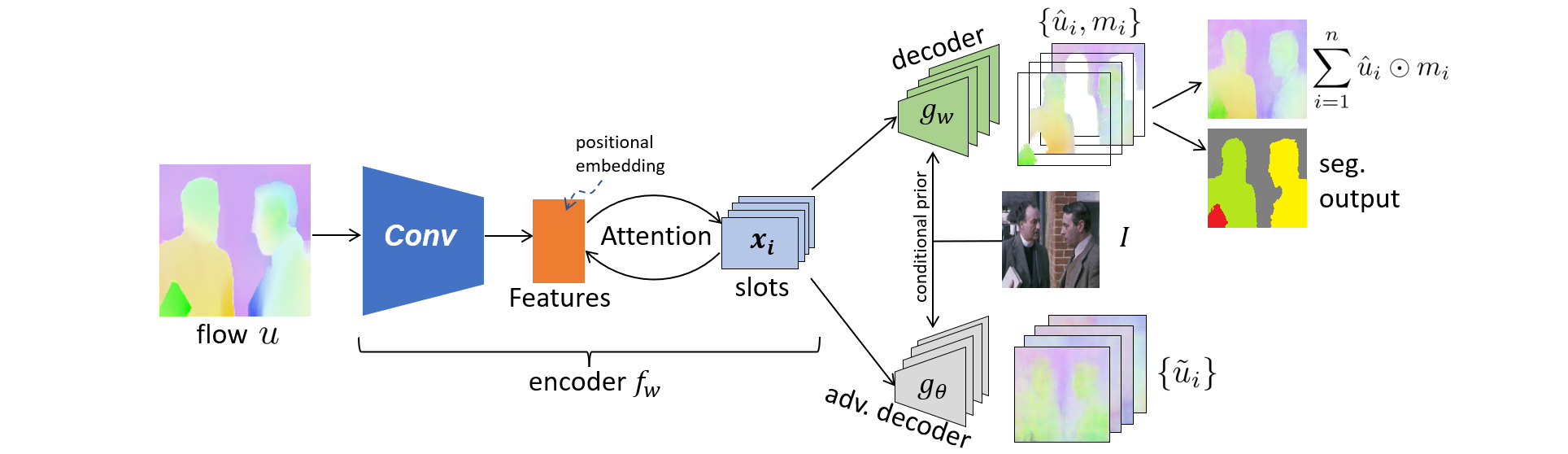
Figure 1: Divided Attention Overview. Unlike traditional autoencoders that process the input (here the flow $u$) through an encoder $f_{w}$, and then reconstruct it through a decoder $g$, DivA uses a cross-modal conditional decoder ($g_{w}$ in green) that takes a second modality as input (here the image $I$) in order to reconstruct the first from the encoding “slots” $x_{i}$ (light blue). The image is used as a condition to guide the flow decoder, using a conditional prior network. To ensure that the individual slots encode separate objects, we incorporate an adversarial decoder ($g_{\theta}$ in grey) that tries to reconstruct the entire flow with each slot. Training is done by optimizing a min-max criterion whereby the model tries to reconstruct the input flow within each object mask, while fooling the adversarial decoder outside. This design enforces information separation between attention slots, leading to Divided Attention. The conditional decoder is expanded in Fig. 2.

1 Introduction

The ability to segment the visual field by motion is so crucial to survival that we share it with our reptilian ancestors. A successful organism should not take too long to learn how to spot predators or obstacles and surely should require no supervision. Yet, in the benchmarks we employ to evaluate multi-object segmentation, the best performing algorithms are trained using large annotated datasets or simulation environments with ground truth. While supervision can certainly be beneficial, we take a minimalistic position and explore the extent in which an entirely unsupervised method can discover multiple objects in images.

To this end, we design a neural network architecture based on Slot Attention Networks (SANs) [26], and train it to segment multiple objects using only an image and its corresponding optical flow, with no other form of supervision. Before we delve into the details, we should clarify that “objects,” in this paper, are regions of an image whose corresponding flow is unpredictable from their surroundings. Objects thus defined approximate the pre-image under optical projection of Gibson’s “detached objects,” which live in the three-dimensional ambient space. This definition is embodied in a variational principle that seeks to partition the image domain into regions that are as uninformative of each other as possible, known as Contextual Information Separation (CIS) [52, 51].

We choose Slot Attention Networks because they structurally organize latent activations into multiple components, or “slots.” However, current SANs combine the slots to minimize the reconstruction error, which does not impose an explicit bias to separate objects into slots. A single slot can reconstruct the entire flow, especially in more complex and realistic scenes where objects are not salient. We hypothesize that the adversarial CIS loss can foster “divided attention” SANs. However, CIS has been applied mostly to binary segmentation, and if an image has a dominant “foreground object” distinct from all others, arguably the discovery problem has already been solved by the individual who framed the image. Naively combining CIS and SANs leads to disappointing results, so modifications of both the architecture and the loss are needed to take these developments beyond the state of the art.

First, to disambiguate multiple partitions in the CIS loss, we modify it to incorporate cross-modal generation: We force the model to reconstruct the flow on the entire image domain, but not the image itself, since most of its complexity can be ascribed to nuisance variability.

Second, we modify SANs to enable the image to guide the flow reconstruction. This is done by incorporating a Conditional Prior Network (CPN) [53], that models the distribution of flows compatible with the given image, and modifying the architecture to use a conditional cross-modal decoder.

We call the resulting method Divided Attention (DivA): It consists of a multi-modal architecture where one modality (flow) goes into the main encoder that feeds the slots, and the other (image) goes into the decoder that generates the flow (Fig. 1), trained adversarially with a loss (2) that captures both cross-modal generation and contextual information separation. These innovations allow us to improve performance on the benchmarks DAVIS and SegTrack by 5% and 7% respectively, compared to recent unsupervised methods, and to close the gap to supervised methods to 9.5% and 12% respectively, all while significantly improving inference speed: An embodiment of DiVA that matches the current state of the art improves speed by 200% (21FPS to 64FPS), and our fastest embodiment reaches 104FPS. DivA can handle a variable number of objects, which can be changed at inference time, and is invariant to permutations of object labels. It does not need explicit regularization, as we demonstrate by using the mean-squared error (MSE) as the base loss.

1.1 Related Work

Unsupervised motion segmentation. Optical flow [15, 36, 38, 40] estimates a dense motion field between frames. To segment it, one can solve a partial differential equation (PDE) [27], group sparse trajectories [30, 18, 19] or decompose it into layers [44, 47, 37, 23]. The number of segments is determined either from user input or through heuristics [39]. However, these methods require processing a video batch and/or solving energy minimization at run time, which makes them impractical at scale.

When using deep neural networks, the number of partitions that a generic segmentation network handles is often determined by the number of output channels [29, 55, 6], which matches with object classes defined by the user. In the absence of pre-defined object classes, many motion segmentation methods [41, 17, 35] perform binary partition into “foreground” and “background,” sometimes referred to as motion saliency [16, 12, 24, 1]. This assumes that the data contain a dominant moving object.

Bootstrapping objects from motion [51, 7] is also related to multi-region segmentation, but again extending binary schemes to multi-region is non-trivial, as there is neither the notion of foreground and background nor an ordering of the regions. Some methods revisit layered models by utilizing supervised training on synthetic data [48] or replacing variational optimization with neural networks [54]. Like older layered decomposition approaches, both require longer video batches. In DivA, we simply use image-flow pairs as model input, which makes it more widely applicable and more efficient at inference time.

Some unsupervised moving object segmentation methods [45, 32] use self-supervised pre-trained image features (e.g. DINO [4]) from ImageNet [9]. Other unsupervised moving object detection methods [2, 3] rely on motion segmentation [8] that leverages supervised image features from MS-COCO [25]. While we are not against any form of pre-training, these methods are tangential to ours. The goal of our work is to explore the limits of fully unsupervised object discovery, given the primal nature of the task. Therefore, we choose to rely on self- and cross-modal consistency as learning criteria without any external pre-training.

Contextual Information Separation (CIS) [52] frames unsupervised motion segmentation as an information separation task. Assuming independence between motions as the defining trait of “objects,” the method segments the optical flow field into two regions that are mutually uninformative. Although still binary partitioning, this formulation removes the notion of foreground and background in motion segmentation. DivA further extends CIS by introducing a reconstruction term, which generalizes CIS to an arbitrary number of regions.

Slot Attention Networks (SANs) infer a set of latent variables each representing an object in the image. So-called “object-centric learning” methods [11, 14, 22, 13, 33, 34] aim to discover generative factors that correspond to parts or objects in the scene, but require solving an iterative optimization at test time; SANs process the data in a feed-forward pass by leveraging the attention mechanism [43] that allocates latent variables to a collection of permutation-invariant slots. SANs are trained to minimize the reconstruction loss, with no explicit mechanism enforcing separation of objects. When objects have distinct features, the low-capacity bottleneck is sufficient to separate objects into slots. However, in realistic images, more explicit biases are needed. To that end, [20] resorts to external cues such as bounding boxes, while [10] employs Lidar, which limits applicability.

DivA modifies the SAN architecture by using a cross-modal conditional decoder, along the lines of [53]. By combining information separation, architectural separation, and conditional generation, DivA fosters better partition of the slots into objects.

DivA is most closely related to [49], which applies SAN for iterative binding to the flow. DivA has two key advantages: [49] is limited to binary segmentation and relies on learned slot initializations, making slots no longer invariant to permutation, which results in poor generalization (Fig. 5). Second, [49] only uses optical flow while DivA employs a conditional cross-modal decoder incorporating image information, which guides the segmentation mask to increased accuracy.

Another recent method [28] learns motion segmentation by fitting the flow to multiple pre-defined motion patterns (e.g., affine, quadratic) using Expectation-Maximization (EM). However, due to the rigidity of the network architecture, one needs to adjust the number of output channels and re-train when changing the number of objects. Note that, due to the same architectural constraint, [50], which employs a variant of CIS, is subject to the same limitations.

2 Method

In this section, we describe the main components of our approach: The SAN architecture in Sect. 2.1, its extension to using a conditional decoder in Sect. 2.2, and the adversarial inference criterion, derived from Contextual Information Separation, in Sect. 2.3.

DivA ingests a color (RGB) image $I\in{\mathbb{R}}^{\mathrm{H}\times\mathrm{W}\times 3}$ with $\mathrm{H}\times\mathrm{W}$ pixels and its associated optical flow $u\in{\mathbb{R}}^{\mathrm{H}\times\mathrm{W}\times 2}$ defined on the same lattice (image domain), and encoded as an RGB image using a color-wheel. DivA outputs a collection of $n$ binary masks $m_{i},\ i=1,\dots,n$ and the reconstructed flow $\hat{u}$.

2.1 Preliminaries: Slot Attention Autoencoder

The DivA architecture comprises a collection of latent codes $X_{n}=\{x_{1},\dots,x_{n}\}$, with each $x_{i}\in{\mathbb{R}}^{1\times K}$ representing a “slot.” The encoder $f_{w}(u)=X_{n}$ is the same as a Slot Attention Network (SAN), described in detail in [26] and summarized here. SANs are trained as autoencoders: An image $I$ is passed through a CNN backbone with an appended positional embedding, but instead of having a single latent vector, SAN uses a collection of them $\{x_{i}|i=1,\cdots,n\}$, called slots, in the bottleneck, where $n$ may change anytime during training or testing. Slots are initially sampled from a Gaussian with learned mean and standard deviation, without conditioning additional variables, including the slot ID. This affords changing the number of slots without re-training, and yields invariance to permutation of the ordering of the slots, which are updated iteratively using dot-product attention normalized over slots, which fosters competition among slots. The result is passed through a Gated Recurrent Unit (GRU) with a multi-layer perceptron (MLP) to yield the update residual for slots. All parameters are shared among slots to preserve permutation symmetry. Each slot is then decoded independently with a spatial broadcast decoder [46] $g$ producing slot reconstructions $\hat{I}_{i}$’s and segmentation masks $m_{i}$’s. The final image reconstruction is $\hat{I}=\sum_{i=1}^{n}\hat{I}_{i}\odot m_{i}$ where $\odot$ denotes element-wise multiplication. SAN is trained by minimizing a reconstruction loss (typically MSE) between $I$ and $\hat{I}$.

2.2 Cross-modal Conditional Slot Decoder

Experimental evidence shows that slots can learn representations of independent simple objects on synthetic images. However, naive use of SAN to jointly auto-encode real-world images and flow leads to poor reconstruction. Since the combined input is complex and the slots are low-dimensional, slots tend to either approximate the entire input or segment the image in a grid pattern that ignores the objects. Both lead to poor separation of objects via the learned slots.

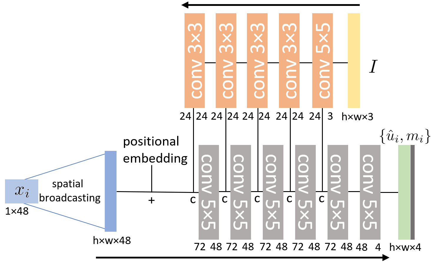
Figure 2: Architecture of the conditional decoder.

For these reasons, we choose not to use the image as input to be reconstructed, but as context to condition the reconstruction of a simpler modality – the one least affected by complex nuisance variability – flow in our case. The conditional decoder $g_{w}$ maps each latent code $x_{i}$ and image $I$ onto a reconstructed flow $\hat{u}_{i}=g_{u}(x_{i},I)$ and a mask $m_{i}=g_{m}(x_{i},I)$. With an abuse of notation, we write $g_{w}=(g_{u},g_{m})$ depending on whether we emphasize its dependency on the weights $w$ or on the component that generates the flow $u$ and the mask $m$ respectively.

This decoder performs cross-modal transfer, since the image is used as a prior for generating the flow. This is akin to a Conditional Prior Network [53], but instead of reconstructing the entire flow, we reconstruct individual flow components (modes) corresponding to objects in the scene indicated by the decoded masks. The reconstructed flow is then obtained as $\hat{u}=\sum_{i=1}^{n}\hat{u}_{i}\odot m_{i}$. In the next section, we will also use an adversarial conditional decoder to generate $\tilde{u}=g_{\theta}(x_{i},I)$, that attempts to reconstruct the entire flow $\tilde{u}$ from each individual slot $x_{i}$, which in turn encourages the separation between different slots.

2.3 Adversarial Learning with Contextual Information Separation

We now describe the separation criterion, which we derive from CIS [51], to divide slots into objects. Each image $I$ and flow $u$ in the training set contribute a term in the loss detailed below:

$$\ell(u,I)=\big{\|}u-\sum_{i=1}^{n}\hat{u}_{i}\odot m_{i}\|\\ -\frac{\lambda}{n}\sum_{i=1}^{n}(1-m_{i})\odot\|u-\tilde{u}_{i}\|$$ (1)

The first term penalizes the reconstruction error by the cross-modal autoencoder combining all the slots, i.e., we want the reconstructed flow to be as good as possible. The second term combines the reconstruction error of the adversarial decoder using a single slot at a time, and maximizes its error outside the object mask. Note that, in the second term, the adversarial decoder $g_{\theta}$ tries to approximate the entire flow $u$ with a single slot $\tilde{u}_{i}=g_{\theta}(x_{i},I)$, which is equivalent to maximizing the contextual information separation between different slots. Also note that we use the mean-square reconstruction error (MSE) $d(u,v)=\|u-v\|_{2}$ for simplicity, but one can replace MSE with any other distance or discrepancy measure such as empirical cross-entropy, without altering the core method. The overall loss, averaged over training samples in a dataset $D$, is then minimized with respect to the parameters $w$ of the encoder $f_{w}$ and conditional decoder $g_{w}$, and maximized with respect to the parameters $\theta$ of the adversarial decoder $g_{\theta}$:

$$\min_{w}\max_{\theta}L(w,\theta)=\sum_{(u_{j},I_{j})\in D}\ell(u_{j},I_{j}).$$ (2)

Compared to CIS, our method is minimizing mutual information between different slots, where the data is encoded, rather than directly between different regions, which eliminates degenerate slots thanks to the reconstruction objective. The resulting design is a natural extension of CIS to non-binary partitions, and also leads to increased versatility: DivA can be trained with a certain number of slots, on images of a certain size, and used at inference time with a different number of slots, on images of different size. Note that the DivA loss does not need explicit regularization, although one can add it if so desired.

Image	Flow	Recon. Flow	Slot1	Slot2	Slot3	Slot4	Segmentation

Figure 3: Multi-region moving object discovery on real data. Our method discovers moving objects in videos without any human annotation or supervision. The slots are randomly initialized, so as to be permutable. We visualize them in a particular order for ease of visualization.

3 Experiments

Encoder. The encoder $f$ consists of 4 convolutional layers with kernel size equal to $5\times 5$, consistent with the original implementation of [26]. With padding, the spatial dimension of the feature map is the same as the network input. Since optical flow is simpler to encode than RGB images, we choose $K=48$ instead of 64 used by the original SAN, resulting in a narrower bottleneck. A learned 48-dimensional positional embedding is then added to the feature map. We tried Fourier positional embedding and the network shows similar behavior. We keep the iterative update of slots the same as the original SAN, and fix the number of slot iterations to be 3.

Conditional decoder and adversarial decoder. The architecture of the conditional decoder $g_{w}$, shown in Fig. 2, consists of two parts: an image encoder, and a flow decoder. We use 5 convolutional layers with filter size {5,3,3,3,3} in the image encoder. Same as $f$, with padding, the size of the feature maps remains the same as $I$. We limit the capacity of this encoder by setting the output channel dimension of each layer to 24 to avoid overfitting the flow to the image, ignoring information from the slots.

The flow decoder takes one $1\times 48$ slot vector $x_{i}$ as input. It first broadcasts $x_{i}$ spatially to $h\times w\times 48$, and adds it to a learned positional embedding. Note that the positional embedding is different from the one in $f$. The broadcasted slot then passes through 6 convolutional layers. The feature map at each layer is concatenated with the image feature at the corresponding level. The last convolutional layer outputs a $h\times w\times 4$ field, where the first 3 channels reconstruct the optical flow, and the 4th channel outputs a segmentation mask. The adversarial decoder shares the same architecture, except for the last layer, which outputs 3 channels aiming to reconstruct the flow on the entire image domain.

Training. We implement implicit differentiation during training as proposed by [5] for stability. We aim to keep the training pipeline simple and all models are trained on a single Nvidia 1080Ti GPU with PyTorch. We apply alternating optimization to $w$ and $\theta$ by Eq. (2). In each iteration, we first fix $g_{\theta}$ and update $w$, then use torch.detach() to stop gradient computation on $x_{i}$ before updating $\theta$. This makes sure that only $\theta$ is updated when training the adversarial decoder. We train with batch size 32 in all experiments and apply the ADAM optimizer with an initial learning rate $8e^{-4}$ and decay schedule for both $w$ and $\theta$. We notice that the model is not sensitive to the choice of learning rate. Further details on training parameters and data normalization are provided in the Supplementary Material.

3.1 Diagnostic data and ablation

	SAN	$\lambda=0$	$\lambda=0.01$	$\lambda=0.03$	$\lambda=0.05$
bIoU	51.18	82.93	84.49	82.33	79.56
SPC	120	133	161	182	174

Table 1: Results on diagnostic data. Conditional decoding significantly improves bootstrapping IoU (bIoU), indicating better awareness of object shape; adversarial training significantly improves successful partition count (SPC), indicating better information separation in slots.

We reproduce the ideal conditions of the experiments reported in [52] to understand the effect of our conditional decoder on the adversarial training scheme. Instead of using binary segmentation masks, we generate flow-image pairs that contain $n=2,3,4$ regions and corresponding statistically independent motion patterns. We adopt object masks from the DAVIS dataset and paste them onto complex background images so that the network cannot overfit to image appearance for reconstruction and segmentation. During training, we fix the number of slots to be 4 and the network is unaware of the number of objects.

We evaluate our models on 300 validation samples and measure the performance by two criteria: bootstrapping IoU (bIoU) and successful partition counts (SPC). We match each ground truth object mask to the most likely segment (with the highest IoU), and then compute bIoU by averaging this IoU across all objects in the dataset. This metric measures how successfully each object is bootstrapped by motion. However, bIoU does not penalize falsely bootstrapped blobs. In addition, SPC counts the number of cases where the number of objects in the segmentation output matches the ground truth number of objects. As the architecture itself is not aware of the number of objects in each flow-image pair during testing, multiple slots may map to the same object. We call this phenomenon slot confusion. A higher SPC is achieved when information is separated among slots, reducing confusion.

Table 1 summarizes the results on these diagnostic data. Our conditional decoder allows exploiting photometric information, in addition to motion, improving bIoU; adversarial learning fosters better separation among slots, reducing slot confusion and improving SPC.

To better understand the role of adversarial training, in Fig. 4 we display the scatter between reconstruction error and segmentation $\text{Mask Entropy}=\sum_{i}^{4}m_{i}\log(m_{i})$ during training. A smaller entropy corresponds to a more certain mask output, indicating that the decoder relies more on single slots to reconstruct optical flow for each particular object. At each level of reconstruction error, the larger $\lambda$, the smaller the mask entropy. This phenomenon is expected since, with information separation, only one slot contains information about the flow of each object, validating our adversarial training. Note that entropy regularization is applied to existing unsupervised segmentation methods (e.g., [49]), and our adversarial loss provides a potential alternative to entropy regularization.

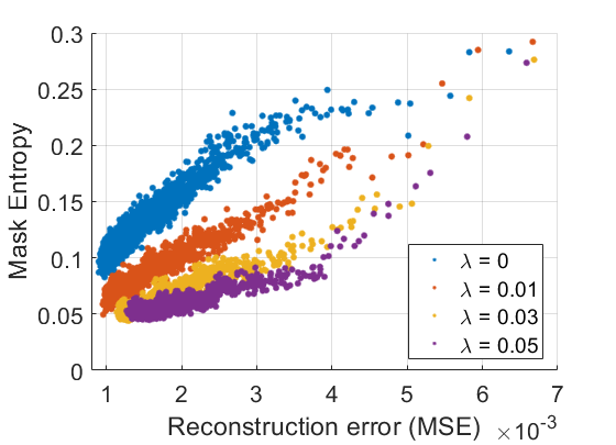
Figure 4: Adversarial loss is an implicit mask entropy regularizer. At each level of reconstruction error, the higher $\lambda$ we apply, the smaller entropy we get in the segmentation output. With the adversarial loss, the model successfully predicts the number of independent motion patterns on more samples.

3.2 Real-world data and benchmark

We first introduce baseline methods we compare with.

CIS [52] uses a conventional binary segmentation network architecture and is trained using the contextual information principle. The method employs an auxiliary flow inpainting network and enforces information separation by minimizing mutual inpainting accuracy on the regions.

Moseg [49] uses a variant of SAN that is tuned for iterative binding to the flow field. The method performs binary segmentation by fixing the number of slots to 2, and learning slot initialization instead of using random Gaussian. The method is trained by reconstruction loss together with temporal consistency loss on videos.

EM [28] uses a conventional segmentation network. During training, the method pre-defines a class of target motion patterns (e.g., affine), and updates the predicted segmentation mask and estimated motion pattern using EM.

We select these methods as paragons since they all 1) use single-frame (instantaneous motion) without exploiting long-range cross-frame data association; 2) do not rely on the presence of a dominant “foreground object,” even though that may improve performance in artificial benchmarks given the bias of human-framed photographs and videos. Our method is chosen so as to be efficient and flexible, leading to 1), and not biased towards purposefully framed videos, leading to 2).

Method	Resolution	Multi	DAVIS	ST	FPS
Unsupervised
CIS [52](4)	$128\times 224$	N	59.2	45.6	10
CIS(4)+CRF	$128\times 224$	N	71.5	62.0	0.09
MoSeg[49]	$128\times 224$	N	65.6	-	78
MoSeg(4)	$128\times 224$	N	68.3	58.6	20
EM* [28]	$128\times 224$	Y*	69.3	60.4	21
DivA	$128\times 128$	Y	68.6	60.3	104
DivA	$128\times 224$	Y	70.8	60.1	64
DivA-Recursive	$128\times 224$	Y	71.0	60.9	66
DivA(4)	$128\times 224$	Y	72.4	64.6	16
With Additional Supervision
FSEG [17]	Full	N	70.7	61.4	-
OCLR [48](30)	$128\times 224$	Y	72.1	67.6	-
ARP [21]	Full	N	76.2	57.2	0.015
DyStab [51]	Full	N	80.0	73.2	-

Table 2: Moving object segmentation on real-world data. Although our model is not specifically designed for binary segmentation, we still achieve state-of-the-art accuracy on DAVIS16 and SegTrackV2 datasets with better inference speed. Multi: generalizes to multiple regions. EM*: Trained unsupervised on synthetic data and needs to alter network architecture and retrain when changing the number of regions.

Datasets. We test our method on DAVIS2016 [31], SegTrackV2 [42] and FBMS59 [30]. DAVIS2016 consists of 50 image sequences ranging from 25 to 100 frames along with high-quality per-pixel segmentation masks. Each video contains one primary moving object that is annotated. We perform training and validation using the 480P resolution. SegtrackV2 has 14 video sequences with a total of 947 frames with per-frame annotation. Annotated objects in the video have apparent motion relative to the background. FBMS-59 dataset contains 59 videos ranging from 19 to 800 frames. In the test set, 69 objects are labeled in the 30 videos. Following the baseline methods, we test our method for binary segmentation on DAVIS2016 and SegTrackV2 by setting $n=2$. On FBMS-59, we make use of per-instance annotations offered by the dataset and test multi-object bootstrapping.

Training and testing. We apply RAFT [40] for optical flow estimation following [49, 28]. For image sequence $\{I_{t}\}$, RAFT computes optical flow from $I_{t}$ to $I_{t+\delta t}$, where $\delta t$ is randomly sampled from -2 to 2. Same to the baselines, optical flow is computed on original resolution images, then downsampled together with the reference image before feeding to the network. During training, we warm up our model on DAVIS2016 dataset, setting $n=4$. During this warm-up stage, we set $\lambda=0$ so that the model can learn reconstruction in the initial stage without the interference of an adversarial decoder. After the warm-up, we train the model on each particular dataset, with $n=2$ on DAVIS2016 and SegtrackV2, and $n=4$ on FBMS-59. Referring to the empirical evidence on the diagnostic dataset, We set $\lambda=0.03$, and decrease it to $\lambda-0.01$ towards the end of the training. We use a batch size of 32 and set the spatial resolution of model input to be $128\times 128$ when $n=4$ and $128\times 224$ when $n=2$, tailored by the GPU’s memory constraint. Details about hyper-parameters and data normalization are in the supplementary material.

At test time, we keep $n=2$ on DAVIS2016 and SegtrackV2, and vary $n$ on FBMS-59. On binary segmentation, since the model is trained without the notion of foreground and background, we follow the baselines to match the ground truth with the most likely segmentation mask and compute intersection-over-union (IoU) to measure the segmentation accuracy. We upsample the segmentation output to the dataset’s original resolution for evaluation. Unlike baseline methods that upsample low-resolution segmentation masks by interpolation, our generative model reconstructs flow from each slot, so we can refine the segmentation outputs by upsampling $\{\hat{u}_{i}\}$’s to the full resolution, then refine the segmentation boundaries by $\operatorname*{arg\,min}_{i}|u-\hat{u}_{i}|_{2}$. This practice creates negligible computational overhead (0.00015s) and empirically improves segmentation accuracy. On multi-object bootstrapping, we follow the bootstrapping IoU defined in Sect. 3.1 and evaluate the accuracy per instance. Note that this is different from the baseline methods that merge all instances into a single foreground for evaluation.

	Input Flow	MoSeg[49]	DivA
Original
Flipped

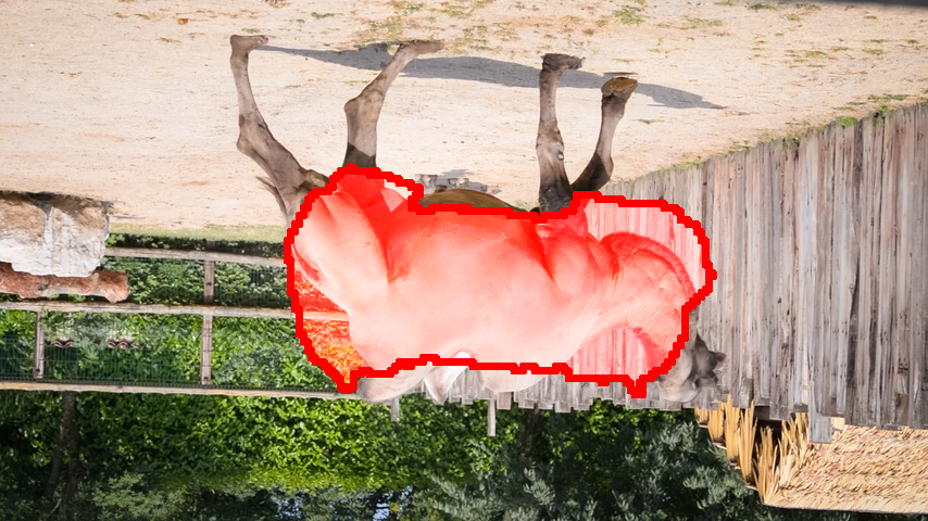
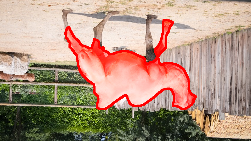
Figure 5: Conditional decoder is less vulnerable to overfitting. Reconstructing complex flow input from compressed slots forces the decoder to overfit to seen data. Simply flipping the input flow drastically decreases segmentation accuracy. By introducing the conditional decoder, DivA is less vulnerable to overfitting.

Results on DAVIS2016 and SegTrackV2 are summarized in Table 2. Our best result outperforms the best-performing baseline EM by 4.5% and 6.9%, respectively. We measure the run time of one single forward pass of the model. Our fastest setting using $128\times 128$ spatial resolution reaches 104 frames per second. Note that in addition to running on consecutive frames, CIS and MoSeg merge segmentation results on optical mapping from the reference frame to 4 adjacent temporal frames ($\delta t$ = -2,-1,1 and 2), marked by “(4)” in the table. The same protocol improves our mIoU on both datasets by 1.4 and 3.7, respectively. Compared to models using additional supervision, our best performance exceeds the FSEG [17] (supervised) and OCLR [48] (supervised, trained on synthetic data), and closes the gap with the best-performing method DyStab [51] (with supervised image feature) to 12%.

Inspired by [10], we also test DivA by recursively inheriting slots from the previous frames instead of randomly initializing them, and reducing the number of slot iterations from 3 to 1. Both segmentation accuracy and runtime speed improve marginally. The base model randomly assigns labels to the foreground and background; with recursion, label-flipping is reduced. Unlike MoSeg and DyStab that employ explicit regularization mechanisms, our method exhibits temporal consistency without any modification to the training pipeline.

Furthermore, we compare the model pipelines of MoSeg and DivA, both of which use slot attention. MoSeg only takes flow as input. Without the conditional decoder, due to the highly compressed bottleneck of each slot, the network relies on the decoder’s capacity to reconstruct fine structures of the input flow. This mechanism forces the decoder to memorize shape information. Together with learned slot initializations, the network is subject to overfitting to the data seen during training. Fig. 5 shows an example, where simply flipping the input image leads to performance degradation. Conditioning the decoder on the image frees it from memorizing training data to be reconstructed, thus making the model less vulnerable to overfitting.

	$\delta t=1$			$\delta t=2$
n	SAN	w/cond.	DivA	SAN	w/cond.	DivA
3	17.76	39.81	40.87	17.66	40.90	41.27
4	19.27	40.96	42.54	19.57	39.81	41.85
5	20.17	38.73	40.25	20.15	38.47	40.48
6	19.69	38.03	38.90	17.90	38.59	40.26

Table 3: Bootstrapping accuracy on FBMS-59. We evaluate the performance of DivA on FBMS-59 by bIoU, varying the number of slots in the network (without re-training). We report results on the baseline SAN [26], SAN with our conditional decoder, and the full DivA model.

Results on FBMS-59. We demonstrate DivA’s performance on multi-object discovery using FBMS-59. We train with $n=4$ aiming to extract multiple independently moving objects from a scene. At test time, we vary $n$ ranging from 3 to 6 without re-training the model, and report bootstrapping IoU. We test the model on optical flow computed with $\delta t=1$ and $\delta t=2$, and keep the spatial resolution to $128\times 128$ in both training and testing.

We use the original SAN as the baseline, and also include results combining SAN with the conditional decoder, as in Sect. 3.1. Table 3 summarizes the results. Similar to Sect. 3.1, the conditional decoder improves segmentation accuracy substantially, and the adversarial training further improves accuracy by 3.9% in the best-performing case. We notice that $n=4$ is a sweet spot for the dataset, due to the dataset’s characteristic of having around 3 moving objects in most sequence. Fig. 3 shows qualitative examples.

For many objects segmented, we observe a change in the level of granularity of the segmentation mask when varying $n$. Two examples are given in Fig. 6. Although depending on the annotation, both cases may be considered as over-segmenting the object in quantitative evaluations and may degrade IoU, we argue that such behavior is desirable. As our model can vary the number of slots without re-training, it reveals DivA’s potential in developing adaptive, interactive, or hierarchical segmentation schemes in future work.

Image	Optical Flow	2 slots	3 slots	4 slots

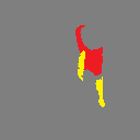
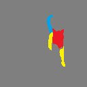
Figure 6: Varying the number of slots changes the granularity of segmentation. All the above results are obtained by only varying the number of slots at inference time without re-training. This gives users additional control over the granularity of segmentation.

4 Discussion

DivA is a multi-object discovery model trained to perform contextual information separation and cross-modal validation, with no manual supervision. The architecture is based on Slot Attention Networks, but modified to comprise a cross-modal decoder, turning a simple autoencoder into a conditional encoder, and an adversarial decoder. The loss function uses the adversarial decoder to enforce Contextual Information Separation but not directly in the data, but in the latent space of the slot encodings.

The overall system enjoys certain properties not observed in current methods: First, it does not require specifying the number of objects, and allows for their upper bound to change between training and test time. Second, the labels are permutation invariant, so DivA can be used in a recursive fashion to reduce label flipping. We can use slots from previous frames as initialization for incoming frames, and only run one slot iteration. Other methods for doing so [10] require manual input and modification of the training pipeline or require consistency heuristics to ensure temporal continuity [51, 49]. Third, the model can be trained on images of a certain resolution, and then used on images of different resolutions at inference time. We have tested training on $128\times 128$ images to spare GPU memory, and testing on $128\times 224$ for accuracy, and vice-versa one can train on larger images and use at reduced resolution for speed. Fourth, DivA does not require sophisticated initialization: It is trained on randomly initialized slots and random image-flow pairs, and tested recursively using slots from the previous frame to initialize for the new frame. It is trained with 4 slots, and tested with 3, 4, 5 and 6 slots, capturing most of the objects in common benchmarks. Fifth, DivA is fast. All our models are trained on a single GPU, and perform at multiples of frame-rate at test time. Finally, since DivA is a generative model, it can be used to generate segmentation masks at high resolution, by upsampling the decoded slots to the original resolution.

Image	Flow	Reconstruction	Segmentation

Figure 7: Failure modes. DivA is trained using the CIS principle, which assumes objects move independently. Consequently, two objects moving in the same way may share high mutual information, e.g., even though the car and the bus are different detached objects, if their motions are highly correlated in the current video, they are seen as one by DivA (of course, as time goes by, their motions will diverge, allowing DivA to correctly separate them).

Some failure cases are shown in Fig. 7. While we have tested DivA on a handful of objects in benchmark datasets, scaling to hundreds or more slots is yet untested. There are many variants possible to the general architecture of Fig. 1, including using Transformer models (e.g. [33, 34]) in lieu of the conditional prior network. With more powerful multi-modal decoders, the role of motion may become diminished, but the question of how the large model is trained (currently with aligned visual-textual pairs), remains. Since our goal is to understand the problem of object discovery ab ovo, we keep our models minimalistic to be trained efficiently even if they do not incorporate the rich semantics of natural language or human-generated annotations.

We can envision several extensions of DivA. For example, even though the amphibian visual system requires objects to move in order to spot them, primate vision can easily detect and describe objects in static images, thus, a bootstrapping strategy can be built from DivA. Moreover, varying the number of slots changes the level of granularity of the slots (Fig. 6), which leads to the natural question of how to extend DivA to hierarchical partitions.

References

- [1] Ijaz Akhter, Mohsen Ali, Muhammad Faisal, and RICHARD HARTLEY. Epo-net: Exploiting geometric constraints on dense trajectories for motion saliency. In Proceedings of the IEEE/CVF Winter Conference on Applications of Computer Vision (WACV), March 2020.
- [2] Zhipeng Bao, Pavel Tokmakov, Allan Jabri, Yu-Xiong Wang, Adrien Gaidon, and Martial Hebert. Discovering objects that can move. In Proceedings of the IEEE/CVF Conference on Computer Vision and Pattern Recognition, pages 11789–11798, 2022.
- [3] Zhipeng Bao, Pavel Tokmakov, Yu-Xiong Wang, Adrien Gaidon, and Martial Hebert. Object discovery from motion-guided tokens. In Proceedings of the IEEE/CVF Conference on Computer Vision and Pattern Recognition, pages 22972–22981, 2023.
- [4] Mathilde Caron, Hugo Touvron, Ishan Misra, Hervé Jégou, Julien Mairal, Piotr Bojanowski, and Armand Joulin. Emerging properties in self-supervised vision transformers. In Proceedings of the IEEE/CVF international conference on computer vision, pages 9650–9660, 2021.
- [5] Michael Chang, Thomas L Griffiths, and Sergey Levine. Object representations as fixed points: Training iterative inference algorithms with implicit differentiation. In ICLR2022 Workshop on the Elements of Reasoning: Objects, Structure and Causality, 2022.
- [6] Liang-Chieh Chen, George Papandreou, Iasonas Kokkinos, Kevin Murphy, and Alan L Yuille. Deeplab: Semantic image segmentation with deep convolutional nets, atrous convolution, and fully connected crfs. IEEE transactions on pattern analysis and machine intelligence, 40(4):834–848, 2017.
- [7] Subhabrata Choudhury, Laurynas Karazija, Iro Laina, Andrea Vedaldi, and Christian Rupprecht. Guess what moves: unsupervised video and image segmentation by anticipating motion. arXiv preprint arXiv:2205.07844, 2022.
- [8] Achal Dave, Pavel Tokmakov, and Deva Ramanan. Towards segmenting anything that moves. In Proceedings of the IEEE/CVF International Conference on Computer Vision Workshops, pages 0–0, 2019.
- [9] Jia Deng, Wei Dong, Richard Socher, Li-Jia Li, Kai Li, and Li Fei-Fei. Imagenet: A large-scale hierarchical image database. In 2009 IEEE conference on computer vision and pattern recognition, pages 248–255. Ieee, 2009.
- [10] Gamaleldin Fathy Elsayed, Aravindh Mahendran, Sjoerd van Steenkiste, Klaus Greff, Michael Curtis Mozer, and Thomas Kipf. Savi++: Towards end-to-end object-centric learning from real-world videos. In Advances in Neural Information Processing Systems.
- [11] SM Eslami, Nicolas Heess, Theophane Weber, Yuval Tassa, David Szepesvari, Geoffrey E Hinton, et al. Attend, infer, repeat: Fast scene understanding with generative models. Advances in neural information processing systems, 29, 2016.
- [12] Deng-Ping Fan, Wenguan Wang, Ming-Ming Cheng, and Jianbing Shen. Shifting more attention to video salient object detection. In Proceedings of the IEEE/CVF Conference on Computer Vision and Pattern Recognition (CVPR), June 2019.
- [13] Klaus Greff, Raphaël Lopez Kaufman, Rishabh Kabra, Nick Watters, Christopher Burgess, Daniel Zoran, Loic Matthey, Matthew Botvinick, and Alexander Lerchner. Multi-object representation learning with iterative variational inference. In International Conference on Machine Learning, pages 2424–2433. PMLR, 2019.
- [14] Klaus Greff, Sjoerd Van Steenkiste, and Jürgen Schmidhuber. Neural expectation maximization. Advances in Neural Information Processing Systems, 30, 2017.
- [15] Berthold KP Horn and Brian G Schunck. Determining optical flow. Artificial intelligence, 17(1-3):185–203, 1981.
- [16] Yuan-Ting Hu, Jia-Bin Huang, and Alexander G Schwing. Unsupervised video object segmentation using motion saliency-guided spatio-temporal propagation. In Proceedings of the European conference on computer vision (ECCV), pages 786–802, 2018.
- [17] Suyog Jain, Bo Xiong, and Kristen Grauman. Fusionseg: Learning to combine motion and appearance for fully automatic segmention of generic objects in videos. arXiv preprint arXiv:1701.05384, 2017.
- [18] Margret Keuper, Bjoern Andres, and Thomas Brox. Motion trajectory segmentation via minimum cost multicuts. In Proceedings of the IEEE international conference on computer vision, pages 3271–3279, 2015.
- [19] Margret Keuper, Siyu Tang, Yu Zhongjie, Bjoern Andres, Thomas Brox, and Bernt Schiele. A multi-cut formulation for joint segmentation and tracking of multiple objects. arXiv preprint arXiv:1607.06317, 2016.
- [20] Thomas Kipf, Gamaleldin F Elsayed, Aravindh Mahendran, Austin Stone, Sara Sabour, Georg Heigold, Rico Jonschkowski, Alexey Dosovitskiy, and Klaus Greff. Conditional object-centric learning from video. arXiv preprint arXiv:2111.12594, 2021.
- [21] Yeong Jun Koh and Chang-Su Kim. Primary object segmentation in videos based on region augmentation and reduction. In 2017 IEEE conference on computer vision and pattern recognition (CVPR), pages 7417–7425. IEEE, 2017.
- [22] Adam Kosiorek, Hyunjik Kim, Yee Whye Teh, and Ingmar Posner. Sequential attend, infer, repeat: Generative modelling of moving objects. Advances in Neural Information Processing Systems, 31, 2018.
- [23] Dong Lao and Ganesh Sundaramoorthi. Extending layered models to 3d motion. In Proceedings of the European conference on computer vision (ECCV), pages 435–451, 2018.
- [24] Haofeng Li, Guanqi Chen, Guanbin Li, and Yizhou Yu. Motion guided attention for video salient object detection. In Proceedings of the IEEE/CVF International Conference on Computer Vision (ICCV), October 2019.
- [25] Tsung-Yi Lin, Michael Maire, Serge Belongie, James Hays, Pietro Perona, Deva Ramanan, Piotr Dollár, and C Lawrence Zitnick. Microsoft coco: Common objects in context. In Computer Vision–ECCV 2014: 13th European Conference, Zurich, Switzerland, September 6-12, 2014, Proceedings, Part V 13, pages 740–755. Springer, 2014.
- [26] Francesco Locatello, Dirk Weissenborn, Thomas Unterthiner, Aravindh Mahendran, Georg Heigold, Jakob Uszkoreit, Alexey Dosovitskiy, and Thomas Kipf. Object-centric learning with slot attention. Advances in Neural Information Processing Systems, 33:11525–11538, 2020.
- [27] Etienne Mémin and Patrick Pérez. Hierarchical estimation and segmentation of dense motion fields. International Journal of Computer Vision, 46:129–155, 2002.
- [28] Etienne Meunier, Anaïs Badoual, and Patrick Bouthemy. Em-driven unsupervised learning for efficient motion segmentation. IEEE Transactions on Pattern Analysis and Machine Intelligence, 2022.
- [29] Hyeonwoo Noh, Seunghoon Hong, and Bohyung Han. Learning deconvolution network for semantic segmentation. In Proceedings of the IEEE international conference on computer vision, pages 1520–1528, 2015.
- [30] Peter Ochs, Jitendra Malik, and Thomas Brox. Segmentation of moving objects by long term video analysis. IEEE transactions on pattern analysis and machine intelligence, 36(6):1187–1200, 2013.
- [31] Federico Perazzi, Jordi Pont-Tuset, Brian McWilliams, Luc Van Gool, Markus Gross, and Alexander Sorkine-Hornung. A benchmark dataset and evaluation methodology for video object segmentation. In Proceedings of the IEEE conference on computer vision and pattern recognition, pages 724–732, 2016.
- [32] Georgy Ponimatkin, Nermin Samet, Yang Xiao, Yuming Du, Renaud Marlet, and Vincent Lepetit. A simple and powerful global optimization for unsupervised video object segmentation. In Proceedings of the IEEE/CVF Winter Conference on Applications of Computer Vision, pages 5892–5903, 2023.
- [33] Gautam Singh, Fei Deng, and Sungjin Ahn. Illiterate dall-e learns to compose. arXiv preprint arXiv:2110.11405, 2021.
- [34] Gautam Singh, Yi-Fu Wu, and Sungjin Ahn. Simple unsupervised object-centric learning for complex and naturalistic videos. arXiv preprint arXiv:2205.14065, 2022.
- [35] Hongmei Song, Wenguan Wang, Sanyuan Zhao, Jianbing Shen, and Kin-Man Lam. Pyramid dilated deeper convlstm for video salient object detection. In Proceedings of the European conference on computer vision (ECCV), pages 715–731, 2018.
- [36] Deqing Sun, Stefan Roth, and Michael J Black. Secrets of optical flow estimation and their principles. In 2010 IEEE computer society conference on computer vision and pattern recognition, pages 2432–2439. IEEE, 2010.
- [37] Deqing Sun, Erik Sudderth, and Michael Black. Layered image motion with explicit occlusions, temporal consistency, and depth ordering. Advances in Neural Information Processing Systems, 23, 2010.
- [38] Deqing Sun, Xiaodong Yang, Ming-Yu Liu, and Jan Kautz. Pwc-net: Cnns for optical flow using pyramid, warping, and cost volume. In Proceedings of the IEEE conference on computer vision and pattern recognition, pages 8934–8943, 2018.
- [39] Brian Taylor, Vasiliy Karasev, and Stefano Soatto. Causal video object segmentation from persistence of occlusions. In Proceedings of the IEEE Conference on Computer Vision and Pattern Recognition, pages 4268–4276, 2015.
- [40] Zachary Teed and Jia Deng. Raft: Recurrent all-pairs field transforms for optical flow. In Computer Vision–ECCV 2020: 16th European Conference, Glasgow, UK, August 23–28, 2020, Proceedings, Part II 16, pages 402–419. Springer, 2020.
- [41] P. Tokmakov, K. Alahari, and C. Schmid. Learning video object segmentation with visual memory. In ICCV, 2017.
- [42] David Tsai, Matthew Flagg, Atsushi Nakazawa, and James M Rehg. Motion coherent tracking using multi-label mrf optimization. International journal of computer vision, 100:190–202, 2012.
- [43] Ashish Vaswani, Noam Shazeer, Niki Parmar, Jakob Uszkoreit, Llion Jones, Aidan N Gomez, Łukasz Kaiser, and Illia Polosukhin. Attention is all you need. Advances in neural information processing systems, 30, 2017.
- [44] John YA Wang and Edward H Adelson. Representing moving images with layers. IEEE transactions on image processing, 3(5):625–638, 1994.
- [45] Yangtao Wang, Xi Shen, Yuan Yuan, Yuming Du, Maomao Li, Shell Xu Hu, James L Crowley, and Dominique Vaufreydaz. Tokencut: Segmenting objects in images and videos with self-supervised transformer and normalized cut. arXiv preprint arXiv:2209.00383, 2022.
- [46] Nicholas Watters, Loic Matthey, Christopher P Burgess, and Alexander Lerchner. Spatial broadcast decoder: A simple architecture for learning disentangled representations in vaes. arXiv preprint arXiv:1901.07017, 2019.
- [47] Yair Weiss and Edward H Adelson. A unified mixture framework for motion segmentation: Incorporating spatial coherence and estimating the number of models. In Proceedings CVPR IEEE Computer Society Conference on Computer Vision and Pattern Recognition, pages 321–326. IEEE, 1996.
- [48] Junyu Xie, Weidi Xie, and Andrew Zisserman. Segmenting moving objects via an object-centric layered representation. In Advances in Neural Information Processing Systems, 2022.
- [49] Charig Yang, Hala Lamdouar, Erika Lu, Andrew Zisserman, and Weidi Xie. Self-supervised video object segmentation by motion grouping. In Proceedings of the IEEE/CVF International Conference on Computer Vision, pages 7177–7188, 2021.
- [50] Yanchao Yang, Yutong Chen, and Stefano Soatto. Learning to manipulate individual objects in an image. In Proceedings of the IEEE/CVF Conference on Computer Vision and Pattern Recognition, pages 6558–6567, 2020.
- [51] Yanchao Yang, Brian Lai, and Stefano Soatto. Dystab: Unsupervised object segmentation via dynamic-static bootstrapping. In Proceedings of the IEEE/CVF Conference on Computer Vision and Pattern Recognition, pages 2826–2836, 2021.
- [52] Yanchao Yang, Antonio Loquercio, Davide Scaramuzza, and Stefano Soatto. Unsupervised moving object detection via contextual information separation. In Proceedings of the IEEE/CVF Conference on Computer Vision and Pattern Recognition, pages 879–888, 2019.
- [53] Yanchao Yang and Stefano Soatto. Conditional prior networks for optical flow. In Proceedings of the European Conference on Computer Vision (ECCV), pages 271–287, 2018.
- [54] Vickie Ye, Zhengqi Li, Richard Tucker, Angjoo Kanazawa, and Noah Snavely. Deformable sprites for unsupervised video decomposition. In IEEE Conference on Computer Vision and Pattern Recognition (CVPR), June 2022.
- [55] Hengshuang Zhao, Jianping Shi, Xiaojuan Qi, Xiaogang Wang, and Jiaya Jia. Pyramid scene parsing network. In Proceedings of the IEEE conference on computer vision and pattern recognition, pages 2881–2890, 2017.